rail freight forecasts: scenarios for 2033/34 and 2043/44 · rail freight forecasts: scenarios for...
TRANSCRIPT

Rail freight forecasts: Scenarios for 2033/34 & 2043/44.
July 2019
Ref: 218007r3_10

© MDS TRANSMODAL LIMITED 2019
CONTENTS
EXECUTIVE SUMMARY ........................................................................................................... 1
1. INTRODUCTION .............................................................................................................. 10
2. ASSUMPTIONS ............................................................................................................... 13
2.1 General assumptions (all commodities) ........................................................................................ 13 2.2 Commodity-specific assumptions .................................................................................................. 16 2.3 Rail-served warehousing sites........................................................................................................ 22 2.4 Scenario F: “Internalisation of Externalities” ................................................................................. 25 2.5 Tonnes per train by sector .............................................................................................................. 26 2.6 Path utilisation, days per week and hours per day ...................................................................... 28 2.7 Other assumptions ........................................................................................................................... 29
3. METHODS AND MODELS EMPLOYED ........................................................................ 31
3.1 Establishing base year traffics ........................................................................................................ 31 3.2 GB Freight Model (GBFM) .............................................................................................................. 31 3.3 Intermodal .......................................................................................................................................... 32 3.3.1 Maritime containers ........................................................................................................................ 32 3.3.2 Assumptions for Domestic (non-port) intermodal ....................................................................... 35 3.3.3 Channel Tunnel through-rail intermodal containers ................................................................... 35 3.3.4 Methodology for intermodal containers and swap bodies ......................................................... 35 3.3.5 Cost models and mode share ....................................................................................................... 36 3.3.6 Integrating the model’s results with present day traffics ........................................................... 37 3.4 Modelling limitations ......................................................................................................................... 37 3.4.1 Comparison to ORR published tonnes lifted figures .................................................................. 38
4. SUMMARY RESULTS ..................................................................................................... 39
4.1 Historical context .............................................................................................................................. 39 4.2 Forecasts ........................................................................................................................................... 42 4.3 Comparison with Freight Market Study (FMS) ............................................................................. 67
5. COMMENTARY ON FORECAST RESULTS ................................................................. 70
5.1 Coal & Biomass ................................................................................................................................ 70 5.2 Construction materials ..................................................................................................................... 70 5.3 Intermodal .......................................................................................................................................... 71 5.4 Other commodities ........................................................................................................................... 71 5.5 Potential new markets ..................................................................................................................... 72
6. ASSIGNMENTS TO THE RAIL NETWORK ................................................................... 73
7. RAIL MARKET SHARES ................................................................................................ 78
8. SENSITIVITY TEST G: A “EUROPEAN GAUGE” FREIGHT ROUTE.......................... 86
9. CONCLUSION ................................................................................................................. 88

Rail freight forecasts: Scenarios for 2033/34 & 2043/44 report Page 1
Our Ref: 218007r3_10_output3 report 2033 2043
EXECUTIVE SUMMARY
This report by MDS Transmodal (MDST) was commissioned by Network Rail and presents forecasts of
rail freight in Great Britain for 2033/34 and 2043/44. It also presents forecasts for 2023/24, extracted
from the equivalent report for 2023/24, which was finalised in May 2018. This report, for 2033/34
and 2043/44, combined with the May 2018 report for 2023/24, represent an update of the forecasts
in Network Rail’s 2013 Freight Market Study.
Over the period since 2004/05, total rail freight lifted has fallen from 115m tonnes to 86m tonnes in
2016/17. However, this is primarily a consequence of the Government’s decision to phase out
electricity generation by coal in order to meet international obligations on CO2 emissions. A limited
volume of biomass traffic has replaced some of the coal despatched by rail to the power stations. Coal
accounts for under 1% of road freight but in 2004/05 coal to power stations (ESI coal) accounted for
35% of all rail freight lifted.
Traffic excluding ESI coal and biomass fell from 74.7m tonnes in 2004/05 to 67.7m tonnes in 2012/13,
largely reflecting a decline in UK heavy industry and in the steel industry in particular. However, since
then traffic excluding ESI coal and biomass has grown to 73.0m tonnes (+8%). Reflecting the decline
in indigenous heavy industry, over the 12 years from 2004/05 to 2016/17 that are covered in the
report (for which consistent rail freight volumes were available), HGV vehicle kms fell by 9% while rail
freight excluding ESI coal and biomass fell by only 2%. This suggests that rail (excluding the energy
supply industry) has grown its market share versus road.
These flows are summarised in the table below.
Table 1: GB rail freight and road freight, 2004/05 to 2016/17
2004/05 2008/09 2012/13 2016/17
ESI Coal + biomass rail tonnes (million) 41 45 47 13
Other rail tonnes (million) 75 71 68 73
Total rail tonnes (million) 115 117 115 86
Index: Other rail tonnes (million) 100 95 91 98
HGV kms (Billions) 29.3 28.6 25.0 26.8
Index all HGV kms 100 98 85 91
Sources: Rail: MDS Transmodal processing of Network Rail data. HGV kms: Transport Statistics Great
Britain (TSGB) for the calendar years 2004, 2008, 2012 and 2016 respectively.
For each sector there are six main capacity-unconstrained scenarios for 2033/34 and 2043/44 – with
assumptions that vary by sector. The scenarios are comprised of an equivalent of the 4 scenarios (A-
D) that were used for 2023/24:

Rail freight forecasts: Scenarios for 2033/34 & 2043/44 report Page 2
Our Ref: 218007r3_10_output3 report 2033 2043
Table 2: The four scenarios reflecting low and high market growth and favourability towards rail
Low market growth High market growth
Factors which favour rail relative to road Scenario A Scenario B
Factors which disfavour rail relative to road Scenario C Scenario D
along with:
• Scenario E: “Base” or “Central” scenario – reflecting a “Do Minimum” mind-set with central
case assumptions.
• Scenario F: “Internalisation of externalities” – whereby users of both road and rail pay their
full external costs. This is built on scenario E.
A sensitivity test G (2043/4 only) is also modelled: The introduction of a new European gauge freight
route between Scotland and the Channel Tunnel Rail Link (CTRL) in East London.
Both the FMS and these latest projections are forecasts of demand – i.e. they are unconstrained by
capacity limits. They assume the levels of service provided by the network in terms of end-to-end
transit times remain constant, relative to the base year (2016/17). Similarly the gauge clearance
capability of the network is assumed to remain constant relative to the base year, except in relation
to certain new warehousing sites and under sensitivity test G.

Rail freight forecasts: Scenarios for 2033/34 & 2043/44 report Page 3
Our Ref: 218007r3_10_output3 report 2033 2043
The results of the 2033/34 and 2043/44 scenarios are shown below (tonnes and total tonne kms). The
equivalent 2023/24 forecasts from the May 2018 report are also shown first in italics (these are the
unconstrained scenarios A2 to D2):
Table 3: Rail freight TONNES forecast for 2023/24 scenarios by sector. Thousand tonnes per year
Sector Actual
2016/17
2023/24
A2
2023/24
B2
2023/24
C2 2023/24 D2
Ports Intermodal 16,213 24,252 27,133 15,320 17,077
Domestic Intermodal 2,481 8,009 8,606 3,281 3,493
Channel Tunnel Intermodal 374 529 578 420 458
ESI Coal 6,284 - - - -
Biomass 6,470 8,464 13,045 8,464 13,045
Waste 1,226 1,165 1,287 1,165 1,287
Construction materials 24,286 33,133 43,383 22,887 29,967
of which spoil 735 997 1,306 733 960
Petroleum 4,710 4,822 5,330 4,470 4,940
Chemicals 899 934 1,032 863 954
Industrial Minerals 1,335 1,580 1,747 1,162 1,284
Metals 7,441 8,226 9,092 6,965 7,698
Automotive 450 468 583 437 548
Ores 4,259 4,046 4,472 4,046 4,472
Coal Other 1,955 1,857 4,052 1,857 4,052
Other 334 368 407 319 353
Empty returns for
containers carrying bulks 413 397 439 393 434
NR Engineering 6,657 6,324 6,990 6,324 6,990
Total 85,786 104,574 128,175 78,371 97,052
Total tonne KILOMETRES
(million) 18,962 23,923 28,472 17,502 21,152
Scenario B2 shows the largest growth in tonnes (+49% overall) – particularly for the construction, and
intermodal sectors. Scenario C2 shows a slight decline (9%). This is mostly accounted for by the
decline in ESI (power station) coal.

Rail freight forecasts: Scenarios for 2033/34 & 2043/44 report Page 4
Our Ref: 218007r3_10_output3 report 2033 2043
Table 4: Rail freight TONNES forecast for 2033/34 scenarios by sector. Thousand tonnes per year
Sector Actual
2016/17
2033/34
A
2033/34
B
2033/34
C
2033/34
D
2033/34
E
2033/34
F
Ports Intermodal 16,213 38,505 42,549 25,920 28,759 31,756 47,832
Domestic
Intermodal 2,481 10,096 12,440 3,311 4,576 6,046 18,465
Channel Tunnel
Intermodal 374 690 773 534 598 621 930
ESI Coal 6,284 - - - - - -
Biomass 6,470 5,013 10,026 5,013 10,026 7,520 7,520
Waste 1,226 1,165 1,287 1,165 1,287 1,226 1,226
Construction
materials 24,286 36,348 45,410 23,028 28,769 35,869 51,277
of which spoil 735 1,075 1,344 507 633 1,060 1,428
Petroleum 4,710 4,891 5,406 4,611 5,097 5,025 5,391
Chemicals 899 949 1,048 866 958 968 1,082
Industrial Minerals 1,335 1,618 1,789 1,177 1,301 1,518 1,858
Metals 7,441 8,455 9,345 7,281 8,047 8,433 9,319
Automotive 450 487 538 461 509 493 549
Ores 4,259 4,046 4,472 4,046 4,472 4,259 4,259
Coal Other 1,955 1,857 4,052 1,857 4,052 1,955 1,955
Other 334 404 446 343 380 383 385
Empty returns for
containers carrying
bulks
413 400 443 395 437 418 418
NR Engineering 6,657 6,324 6,990 6,324 6,990 6,657 6,657
Total 85,786 121,248 147,013 86,333 106,258 113,145 159,122
Total tonne
KILOMETRES
(million)
18,962 30,898 36,958 21,428 25,957 27,717 41,443
The central case (scenario E) shows an increase of 32% in tonnes (46% in tonne km), with intermodal
tonnes doubling.

Rail freight forecasts: Scenarios for 2033/34 & 2043/44 report Page 5
Our Ref: 218007r3_10_output3 report 2033 2043
Table 5: Rail freight TONNES forecast for 2043/44 scenarios by sector. Thousand tonnes per year
Sector Actual
2016/17
2043/44
A
2043/44
B
2043/44
C
2043/44
D
2043/44
E
2043/44
F
Ports Intermodal 16,213 51,844 56,596 35,099 39,321 42,879 61,493
Domestic
Intermodal 2,481 16,724 23,633 5,203 9,026 10,933 27,613
Channel Tunnel
Intermodal 374 811 925 641 732 746 1,091
ESI Coal 6,284 - - - - - -
Biomass 6,470 5,013 10,026 5,013 10,026 7,520 7,520
Waste 1,226 1,165 1,287 1,165 1,287 1,226 1,226
Construction
materials 24,286 47,903 72,412 37,782 57,113 53,338 63,182
of which spoil 735 1,294 1,956 1,042 1,575 1,496 1,714
Petroleum 4,710 5,064 5,597 4,833 5,341 5,209 5,459
Chemicals 899 1,009 1,116 928 1,025 1,025 1,109
Industrial Minerals 1,335 1,759 1,944 1,448 1,600 1,732 1,912
Metals 7,441 8,788 9,713 7,950 8,786 8,897 9,460
Automotive 450 497 549 479 529 509 555
Ores 4,259 4,046 4,472 4,046 4,472 4,259 4,259
Coal Other 1,955 1,857 4,052 1,857 4,052 1,955 1,955
Other 334 413 456 355 393 394 396
Empty returns for
containers carrying
bulks
413 401 443 396 438 419 419
NR Engineering 6,657 6,324 6,990 6,324 6,990 6,657 6,657
Total 85,786 153,617 200,212 113,518 151,132 147,696 194,307
Total tonne
KILOMETRES
(million)
18,962 39,124 49,699 27,638 35,786 36,061 51,560
The central case (scenario E) shows an increase of 72% in tonnes (90% in tonne km), with intermodal
tonnes increasing by 186% and construction materials increasing by 120%.
The table and graph below shows how the new 2023/24, 2033/34 and 2043/44 scenarios compare
with the FMS forecasts, along with the historical traffics from 2004/05. It also shows what the FMS
forecasts would have been for 2016/17 if out-turn assumptions for 2016/17 had been input into the
FMS models.

Rail freight forecasts: Scenarios for 2033/34 & 2043/44 report Page 6
Our Ref: 218007r3_10_output3 report 2033 2043
Table 6: Comparison of new forecasts with the FMS
Scenario Million Tonnes
2016/17 actual 85.8
2023/24 A2: Factors favouring rail, low market growth 104.6
2023/24 B2: Factors favouring rail, high market growth 128.2
2023/24 C2: Factors disfavouring rail, low market growth 78.4
2023/24 D2: Factors disfavouring rail, high market growth 97.1
2023/24 Average of A2, B2, C2 & D2 102.0
2023/24 A3: A2 with capacity constraint 101.5
2023/24 B3: B2 with capacity constraint 119.7
2033/34 A: Factors favouring rail, low market growth 121.2
2033/34 B: Factors favouring rail, high market growth 147.0
2033/34 C: Factors disfavouring rail, low market growth 86.3
2033/34 D: Factors disfavouring rail, high market growth 106.3
2033/34 E: Central 113.1
2033/34 F: Internalisation of external costs 159.1
2043/44 A: Factors favouring rail, low market growth 153.6
2043/44 B: Factors favouring rail, high market growth 200.2
2043/44 C: Factors disfavouring rail, low market growth 113.5
2043/44 D: Factors disfavouring rail, high market growth 151.1
2043/44 E: Central 147.7
2043/44 F: Internalisation of external costs 194.3
2012 actual (from FMS) (12 months to the end of September 2012) 112.4
2016/17 forecast from FMS base with 2016/17 assumptions 77.1
Original FMS central case forecast for 2023/24 127.0
Original FMS central case forecast for 2033/34 161.1
Original FMS central case forecast for 2043/44 211.7

Rail freight forecasts: Scenarios for 2033/34 & 2043/44 report Page 7
Our Ref: 218007r3_10_output3 report 2033 2043
Figure 1
Note the “FMS-based forecast of 2016/17” line shows what a forecast of 2016/17 would have been
(77 m tonnes) using
• the FMS base year (12 months to the end of September 2012)
• input assumptions that reflect the true outcome in 2016/17 (such as lower fuel prices)
• the forecasting methods used in the FMS
See the May 2018 report on 2023/24 forecasts for further details.
ESI (power station) coal has historically been a volatile commodity – and is no longer forecast to be
carried by rail in these forecast scenarios. The graph below shows an equivalent graph but with ESI
coal excluded. Note that the graph does include biomass, which reflects conversion of power stations
from coal to biomass.

Rail freight forecasts: Scenarios for 2033/34 & 2043/44 report Page 8
Our Ref: 218007r3_10_output3 report 2033 2043
Figure 2
The FMS forecasts of 2013 were at the top end of the range of our new forecasts. Our new forecasts
show:
• Lower growth in intermodal traffics due to the less favourable revised input assumptions for
rail costs versus road costs (particularly lower fuel costs), and a lower extent to which we
assume rail-served distribution parks will be developed.
• Lower biomass growth (the FMS had 14m tonnes)
• Higher construction materials growth due to a larger assumed growth in the overall market
than previously forecast in the FMS
The forecast assumptions for the 2033/34 and 2043/44 scenarios were agreed with stakeholders using
the available information at the time (October 2018). There may be subsequent changes to some of
these exogenous assumptions prior to publication of the final report which have not been taken into
account in the modelling and quantified results. The forecasts therefore do not reflect changes in
official projections, forecasts and policies since October 2018.
Planned infrastructure upgrades have not been taken into account that could potentially reduce
operational costs along certain routes. The forecasts (and routeings) therefore reflect the network of
early 2017 and do not reflect any upgrades implemented since then or any planned upgrades.

Rail freight forecasts: Scenarios for 2033/34 & 2043/44 report Page 9
Our Ref: 218007r3_10_output3 report 2033 2043
The forecasts do not reflect changes in rail freight volumes between 2016/17 (the base year for the
forecasts) and 2018/19; i.e. the base year has not been updated. The indications are that there has
been little change in total volumes in 2018/19 relative to 2016/17, albeit Lynemouth biomass power
station has come on line – receiving several trains per day as expected in our forecast assumptions.

Rail freight forecasts: Scenarios for 2033/34 & 2043/44 report Page 10
Our Ref: 218007r3_10_output3 report 2033 2043
1. INTRODUCTION
In 2013 MDS Transmodal produced unconstrained rail freight demand forecasts for Network Rail for
2023/24, 2033/34 and 2043/44 for input into their 2013 Freight Market Study (FMS). These had a
model base year of 12 months to the end of September 2012.
These forecasts were originally reported in an April 2013 report to Network Rail and were consulted
upon. Through that process some input assumptions were revised but the forecasting methodology
remained as described in that report.
There have been several exogenous developments since 2013 that were not anticipated in those
projections which have had the effect of adversely affecting the competitive position of rail freight in
the UK. These include:
• Government energy policy changes resulting in a faster reduction in the role of coal fired
power stations and a lower take-up of biomass than expected because of cuts in the level of
financial support available
• Lower fuel price growth and wage growth than expected. Fuel prices have declined in real
terms. The projections had been based on the then projections being made by the DfT.
• Lower rate of build-out of rail served warehousing sites than expected, consequent on the
‘lost years’ of the financial crisis which delayed projects that continue to be ‘live’.
Another factor which may have adversely affected the competitive position of rail freight is the
existence of capacity constraints on the rail network. The FMS forecasts were not capacity constrained
and therefore did not take account of these constraints.
There have also been developments that have resulted in higher-than-projected volumes, particularly
in the market for transporting construction materials.
Overall these developments have meant that the FMS growth projections (for GB rail freight in total)
are not being realised.
Network Rail therefore commissioned MDS Transmodal to produce revised rail freight forecasts for
the year 2023/24, with a base year of 2016/17. The resultant forecasts were consulted upon and final
forecasts with an associated report (“Rail freight forecasts: Scenarios for 2023/24. Final Report”, May
2018. Ref: 217023r11) were produced in May 2018.
Network Rail then commissioned MDS Transmodal to produce revised rail freight forecasts for years
2033/34 and 2043/44 (also with a base year of 2016/17 to be consistent). This report describes the
assumptions, method and the forecast results for 2033/34 and 2043/44. It also includes the May 2018

Rail freight forecasts: Scenarios for 2033/34 & 2043/44 report Page 11
Our Ref: 218007r3_10_output3 report 2033 2043
results for 2023/24 in italics, but the May 2018 report should be considered the main source of
information for the 2023/24 results.
The modelling methodology varies by sector, but the methods used are in most cases the same as
those used in the 2013 forecasts and the 2018 forecasts.
Like the recent 2023/24 forecasts there are several scenarios. These scenarios are intended to give a
range spanning factors favouring rail to factors disfavouring rail, and low market growth to high
market growth:
• 2033/34 & 2043/44 scenario A: Factors which favour rail relative to road, with low market
growth
• 2033/34 & 2043/44 scenario B: Factors which favour rail relative to road, with high market
growth
• 2033/34 & 2043/44 scenario C: Factors which disfavour rail relative to road, with low market
growth
• 2033/34 & 2043/44 scenario D: Factors which disfavour rail relative to road, with high market
growth
• 2033/34 & 2043/44 scenario E: Central assumptions neither favouring nor disfavouring rail
relative to road, with central market growth
• 2033/34 & 2043/44 scenario F: As scenario E, but with internalisation of external costs1
An additional sensitivity test (scenario G in 2043/44) also considers the traffic that would be attracted
to a European gauge freight route between the Channel Tunnel and Central Scotland – see section 8.
As with the FMS and the main scenarios for 2023/24, these 2033/34 and 2043/44 scenarios are NOT
capacity constrained. In reality, unless more capacity is secured for rail freight at capacity-constrained
locations on the network, it is unlikely that high quality paths along preferred routes will be available,
and the unconstrained growth forecast in some scenarios may as a consequence, not be achievable.
The forecasts assume the levels of service provided by the network in terms of end-to-end transit
times remain constant, relative to the base year (2016/17). Similarly the gauge clearance capability
of the network is assumed to remain constant relative to the base year, except in relation to certain
new warehousing sites and under sensitivity test G. The gauge clearance assumptions in relation to
new warehousing sites are discussed under Section 3.2.
The project has involved consultation with key stakeholders (the Freight Operating Companies (FOCs)
Network Rail and DfT) at each stage. Individual interviews with Direct Rail Services (DRS), DB Cargo,
1 We would expect scenario F to have more traffic than scenario E given that road’s externalities are considered greater than rail’s (as per the DfT’s Mode Shift Benefit calculations (MSBs)) such that user costs would increase more for road than rail

Rail freight forecasts: Scenarios for 2033/34 & 2043/44 report Page 12
Our Ref: 218007r3_10_output3 report 2033 2043
Freightliner, GB Railfreight, and Colas were conducted to seek their views on assumptions and market
conditions in each sector.
This report is structured as follows:
• Section 2 describes the assumptions for each scenario
• Section 3 describes the methods and models employed
• Section 4 summarises the results
• Section 5 comments on the results in section 4
• Section 6 describes the assignment of trains and paths to the rail network
• Section 7 gives the rail market shares in each sector
• Section 8 describes the sensitivity test (scenario G) incorporating a European gauge freight
route
• Section 9 concludes the report.

Rail freight forecasts: Scenarios for 2033/34 & 2043/44 report Page 13
Our Ref: 218007r3_10_output3 report 2033 2043
2. ASSUMPTIONS
For each sector there are six main capacity-unconstrained scenarios for 2033/34 and 2043/44 – with
assumptions that vary by sector. The scenarios are comprised of an equivalent of the 4 scenarios (A-
D) that we used for 2023/24:
Table 7: Four scenarios reflecting low and high market growth and favourability towards rail
Low market growth High market growth
Factors which favour rail relative to road Scenario A Scenario B
Factors which disfavour rail relative to road Scenario C Scenario D
along with:
• Scenario E: “Base” or “Central” scenario – reflecting a “Do Minimum” mind-set with central
case assumptions.
• Scenario F: “Internalisation of externalities” – whereby users of both road and rail pay their
full external costs. This is built on scenario E.
• Sensitivity test G (2043/4 only): The introduction of a new European gauge freight route
between Scotland and the Channel Tunnel Rail Link (CTRL) in East London. See section 8
The model outputs for the above scenarios are unconstrained by capacity.
2.1 General assumptions (all commodities) The tables below show the assumptions that were used for 2023/24 in italics (based on data available
in June 2017), along with the assumptions used (with their sources) for scenarios A, B, C, D and E for
2033/34 and 2043/44 based on data available in October 2018.
Note that all % changes are in real terms (i.e. the change in costs, if economy-wide inflation were to
be zero) for the 7 years from the base year (2016/17) to 2023/24, the 17 years from 2016/17 to
2033/34 and the 27 years from 2016/17 to 2043/44.

Rail freight forecasts: Scenarios for 2033/34 & 2043/44 report Page 14
Our Ref: 218007r3_10_output3 report 2033 2043
Table 8: General assumptions (all commodities)
Assumption relative to 2016/17 Year Sc A Sc B Sc C Sc D Sc E
Labour (drivers' wages for road and
rail)
2023/24 +16% for road
+8% for rail +8% -
2033/34
+30% for
road
+22% for rail
+26%
+28% for
road
+24% for rail
2043/44
+58% for
road
+48% for rail
+53%
+55% for
road
+51% for rail
Source: Work value-of-time, WebTAG table A.1.3.2, May 2018 gives +26% and +53% as a central
forecast for 2033/34 and 2043/44 respectively. 2
HGV fuel costs (including duty)
2023/24 +22% +2% -
2033/34 +48% +15% +27%
2043/44 +53% +20% +32%
Source: BEIS Updated energy and emissions projections, January 2018.
Fuel duty for road and rail
2023/24 +5%
2033/34 +17%
2043/44 +28%
Source: Fuel and Electricity Prices and Components, WebTAG table A.1.3.7, May 2018.
Derived rail fuel costs (including duty)
2023/24 +43% -1%
2033/34 +86% +14% +40%
2043/44 +86% +14% +40%
Operational days per week
2023/24 No change
2033/34 No change
2043/44 No change
Train length (and tonnes of cargo per
train) 3
2023/24 +5% No change
2033/34 +5% No change
2043/44 +5% No change
2 The hypothetical scenarios (A & B) that favour rail in terms of reducing rail costs vs road include a higher HGV wage increase vs rail wages. Two explanations for such a possible outcome are as follows:
• A possible Brexit impact whereby it is more difficult to take advantage of low Eastern European HGV wages. This will have little impact on train drivers.
• Currently there is a relatively free market for HGV drivers, with reasonably easy access for new drivers. This is less true for train drivers. In a rail-market-favouring scenario, we are assuming that the train driver market becomes more flexible with a lower cost of employing drivers. This may be brought about by the short-term impact of reduced demand in sectors such as coal
3 We assume that there is no increase in HGV length and weight under any of the scenarios

Rail freight forecasts: Scenarios for 2033/34 & 2043/44 report Page 15
Our Ref: 218007r3_10_output3 report 2033 2043
The forecasts do not take into account the impact of planned infrastructure projects such as East-West
Rail (EWR), and schemes due to be completed by the start of Control Period 6 (2019) such as longer
trains on the Southampton – West Coast Main Line (WCML) route and from the Peak District.
Apart from a possible impact on HGV drivers’ wages, the forecasts do not take account of the impact
of Brexit because there are many uncertainties at this stage. The impact on the rail freight demand
could potentially be positive or negative and impact in several different ways. For example:
• Most unitised trade with Europe is via HGV or unaccompanied road trailer on ferries thus
favouring road transport within GB. European trade in lolo containers typically travels to
regional ports – with the resultant short inland haul typically favouring road. However
unitised trade with the rest of the world typically arrives in lolo containers at the big deep sea
ports (Felixstowe, Southampton, London Gateway) and often has a long journey inland –
which favours rail. A partial transfer of UK trade from European to the rest of the world could
therefore result in more intermodal port traffic by rail
• Customs checks at ports could disadvantage accompanied HGV traffic which would therefore
encourage European traffic to switch to Channel Tunnel through-rail, lolo containers and
unaccompanied ferry routes, which are typically to rail-connected ports
• If Brexit were to reduce economic growth, this could reduce the overall demand for freight
movements.

Rail freight forecasts: Scenarios for 2033/34 & 2043/44 report Page 16
Our Ref: 218007r3_10_output3 report 2033 2043
2.2 Commodity-specific assumptions Note that all % changes are in real terms (i.e. the change in costs, if economy-wide inflation were to
be zero) for the 7 years from the base year (2016/17) to 2023/24, the 17 years from 2016/17 to
2033/34 and the 27 years from 2016/17 to 2043/44.
Table 9: Variable track charges (variable usage, capacity and coal-spillage charges)
Year Commodity Sc A Sc B Sc C Sc D Sc E
2023/24
Construction +16%
As per scenarios A &
B, plus 25% N/A
Chemicals -15%
Domestic Automotive -11%
Domestic Intermodal -5%
Metals +7%
Industrial Minerals +11%
2033/34
and
2043/44
Domestic Automotive -16%
As per scenarios A &
B, plus 25%
As per
scenarios
A & B
Domestic Intermodal +4%
Other +9%
Petroleum +31%
Chemicals +34%
Coal Other +45%
Domestic Waste +46%
Steel +48%
Coal ESI +62%
Industrial Minerals +63%
Iron Ore +73%
Construction Materials +84%
Biomass +93%
Source for 2023/24: “Track Usage Price List”, Network Rail for 2018/19 vs 2016/17, combined with a
distance-and-tonnage-weighted average for each wagon movement in 2016/17. There is an implicit
assumption that the wagon mix will not change.
Sources for 2033/34 & 2043/44:
• “CP6 Track Usage Price List, 1718 prices (July 2018)”, Network Rail for charges to 2023/24 (end
of CP6)
• “2018 periodic review draft determination, Supplementary document – Charges and
incentives: Variable usage charge consultation”, ORR, June 2018, for an indication that the
changes in charges to the end of CP7 (2028/29) would continue at the same rate of increase
as for the 3 final years of CP6. This document also states that the capacity charge and the coal
spillage charge are to be removed in 2019/20 to partly compensate for the increase in variable
usage charge.

Rail freight forecasts: Scenarios for 2033/34 & 2043/44 report Page 17
Our Ref: 218007r3_10_output3 report 2033 2043
We have therefore subtracted the capacity and the coal spillage charge costs from 2019/20 onwards.
Overall this results in the variable track charges paid in 2019/20 being broadly the same as those paid
in 2018/19, although the impacts vary by sector.
The ORR plan to switch from RPI to CPI as the basis for increasing charges in line with inflation. Our
cost models represent real changes (i.e. as though inflation were zero), so using the preferred CPI as
a measure of inflation to increase charges by should give a more accurate representation of the
changes in charges that the industry will experience. We have therefore adopted the CPI-based
forecasts.
Infrastructure Cost Charges (ICCs) (currently Freight Specific Charge and Freight Only Line Charge)
are due to change and are being applied to biomass from 2019/20. However these are levied on
commodities that are deemed to be largely inelastic to changes in track access charges (ESI coal,
Biomass, Ores and the Nuclear industry), and are therefore not included as inputs into the modelled
forecasts.
Note we are not assuming any real terms changes in variable track charges after the end of CP7
(2028/29).

Rail freight forecasts: Scenarios for 2033/34 & 2043/44 report Page 18
Our Ref: 218007r3_10_output3 report 2033 2043
Table 10: Other commodity-specific assumptions
Assumption Year Sc: A Sc: B Sc: C Sc: D Sc: E
Deep-sea unitised trade growth -
for maritime containers
2023/24 +10% +25% +10% +25% -
2033/34 +35% +55% +35% +55% +45%
2043/44 +60% +80% +60% +80% +70%
Source: MDST’s World Cargo Database (WCD version date 27/10/18) for deep sea cargo giving a central
forecast of +45% and +70% for 2033/34 and 2043/44 respectively.
Container port growth for deep sea containers. In line with market demand – with the following port
developments coming on stream one-by-one to cater for demand:
1. London Gateway full use of existing quay
2. Liverpool full use of existing quay
3. London Gateway full development to the west of the existing quay
4. Felixstowe South full development
5. Southampton redevelopment
In 2043/44 scenarios B &D (highest growth), all of these port expansions would be required.
Freightliner’s Tilbury rail traffic is removed
European unitised trade growth
(for short sea (European) trade
including Channel Tunnel
containers)4
2023/24 +10% +20% +10% +20% -
2033/34 +25% +40% +25% +40% +32%
2043/44 +42% +62% +42% +62% +52%
Source: MDST’s World Cargo Database (WCD version date 27/10/18) for European unitised cargo giving
a central forecast of +32% and +52% for 2033/34 and 2043/44 respectively.
4 For Channel tunnel container traffic (between inland GB and inland continental Europe; not Channel Tunnel
shuttle traffic for HGVs), its market is assumed to grow by the forecast European unitised trade growth - e.g.
+52% from 2016/17 to 2043/44 in scenario E.
Additionally factors favouring or disfavouring rail have an impact on Channel Tunnel’s competitiveness versus its competition: container-carrying ships and other unitised services (accompanied HGVs and unaccompanied trailers):
• Fuel and drivers’ wage price changes increase the cost of using the Channel Tunnel, but for shipping services they cause a larger proportional increase in the road costs to get to/from the ports.
• The increase in track charges disfavours Channel Tunnel versus its shipping competition, albeit this increase is only applied to the portion of the haulage within GB.
• Increased train length (scenarios A & B) reduces rail costs and thus favours Channel Tunnel versus its competition
We have NOT included any Channel-Tunnel-specific real-terms changes such as toll reductions, improvements in service quality on the French rail network, or changes to security concerns.

Rail freight forecasts: Scenarios for 2033/34 & 2043/44 report Page 19
Our Ref: 218007r3_10_output3 report 2033 2043
Table 10b: Other commodity-specific assumptions continued
Assumption Year Sc: A Sc: B Sc: C Sc: D Sc: E
Domestic non-bulk traffic market
growth
2023/24 +4.7% +14.2% +4.7% +14.2% -
2033/34 +8.3% +35.3% +8.3% +35.3% +21.8%
2043/44 +11.6%. +68.7% +11.6%. +68.7% +40.2%
Source: Population growth (+8.3%, +11.6%. Source: ONS National Population Projections, October 2017)
and GDP growth (+35.3%, 68.7%. Sources: OBR Economic and Fiscal Outlook, October 2018 and Fiscal
Sustainability Report, July 2018) for 2033/34, 2043/44 respectively. Values for scenario E are the midpoint
of population and GDP growth forecasts.
MSRS grants All Retained Removed
Channel Tunnel bulks growth
for all years All -5% +5% -5% +5%
No
change
Petroleum, Chemicals, Industrial Minerals, Metals and Automotive
No major changes forecast in the overall markets, but fuel prices and drivers’ wages will impact on
rail’s mode share.
Overall market: Low market growth: -5%. High market growth: +5%. Central market growth
(scenario E): No change
Power station (ESI) coal: No rail traffic in 2023/245, 2033/34 and 2043/44
Source for 2033/34 & 2043/44 assumption: BEIS 2017 Updated Energy & Emissions Projections
Annex J (v1.0 21-Nov-2017, Reference scenario) projects that electricity generation by coal will
have declined to zero by 2026.
Biomass: % increase for traffic
to Drax 2033/34 & 2043/44
Low market growth
(Sc A & C): -33%
High market growth
(Sc B & D): +33%6
Base (Sc E):
Stable: 6.5m
tonnes
Lynemouth
2033/34 & 2043/44
Low market growth
(Sc A & C): 0.70m t
High market growth
(Sc B & D): 1.40m t
Base (Sc E):
1.05m tonnes
• Drax traffic is not expected to significantly increase or decrease. However their 4th unit
conversion to biomass gives them the opportunity to increase traffic in the high market
scenario.
5 As described in our May 2018 report, the BEIS projections of January 2017 that we used for our 2023/24 forecasts stated zero electricity generation from coal in 2024. However the November 2017 BEIS projections stated some significant coal-sourced generation remaining - reflecting around 1.6m of ESI coal by rail in 2023/24 (pro rata decrease from 2016 tonnes of ESI coal by rail). Some power station coal traffic by rail is therefore likely to remain in 2023/24 because coal-fired power stations can now continue to run unconstrained to the end of September 2025 if they adhere to the Industrial Emissions Directive (IED) 6 If the recommendations in “Net-Zero – the UK’s Contribution to stopping global warming” (Committee on Climate Change, May 2019) are introduced for biomass in conjunction with carbon capture, growth could be higher than we have assumed in this scenario

Rail freight forecasts: Scenarios for 2033/34 & 2043/44 report Page 20
Our Ref: 218007r3_10_output3 report 2033 2043
• Having started in Spring 2018, Lynemouth appears to be on track to achieve annual biomass
traffics of just over 1 million tonnes.
Table 10c: Other commodity-specific assumptions continued
Assumption relative
to 2016/17 Year Sc: A Sc: B Sc: C Sc: D Sc: E
Construction
materials market
growth
2023/24 +4.7% +14.2% * +4.7% +14.2% * -
2033/34 +8.3% +35.3% +8.3% +35.3% +21.8%
2043/44 +11.6% +68.7% +11.6% +68.7% +40.2%
The low market growth figures (scenarios A & C) are based on population growth (Source: ONS for GB).
The high market growth figures (scenarios B & D) are based on GDP growth (Source: OBR).
Scenario E is the mid-point.
Construction
Construction activity appears to be volatile at present so there is uncertainty about future activity.
Fuel prices and drivers’ wages will impact on rail’s mode share (i.e. scenarios A and B relative to scenarios C
and D). The trend towards super-quarries served by rail may also increase rail’s mode share; however this
may be offset (at the GB level) by an increase in locally sourced secondary/ recycled materials, not served by
rail. We assume that no change in rail market share results from these factors (i.e. that the super-quarries
and recycling factors roughly offset each other).
Waste, Ore, Other Coal, Other and Network Rail Engineering
Rail traffics assumed largely stable into the future
Low market growth: -5%.
High market growth: +5%, plus 2 million tonnes of coking coal from Whitehaven
Central market growth (scenario E): No change
* Note that for 2023/24, under scenarios B and D only, an additional 20% uplift was applied to rail
volumes to reflect the impact of major infrastructure schemes. This is discussed in the May 2018
report. This uplift is not applied to the 2033/34 and 2043/44 forecasts.
These assumptions were chosen using the available information at the time (October 2018). There
may be subsequent changes to some of these exogenous assumptions prior to publication of the final
report which have not been taken into account in the modelling and quantified results.
The forecasts therefore do not reflect changes in other official projections, forecasts and policies since
October 2018, such as labour and fuel cost assumptions.
To be consistent with the 2023/24 forecasts, the base year remains 2016/17. The forecasts do not
reflect changes in rail freight volumes between 2016/17 (the base year for the forecasts) and 2018/19;
i.e. the base year has not been updated to 2018/19. The indications are that there have not been
major changes in volumes in 2018/19 relative to 2016/17 (see table 15 with graph) albeit Lynemouth
biomass power station has come on line – receiving several trains per day.

Rail freight forecasts: Scenarios for 2033/34 & 2043/44 report Page 21
Our Ref: 218007r3_10_output3 report 2033 2043

Rail freight forecasts: Scenarios for 2033/34 & 2043/44 report Page 22
Our Ref: 218007r3_10_output3 report 2033 2043
2.3 Rail-served warehousing sites There are approximately 1 million square metres of new large-scale warehousing (warehouses of
>9,000 square metres) built each year in Britain based on long term trends. We assume around 26%
of this is likely to be rail-served in the rail-favouring scenarios (A and B) - i.e. equating to a build rate
of around 260,000 square metres per year. For the rail dis-favouring scenarios (C and D), we assume
around half the rate of development i.e. 130,000 square metres per year. Scenario E is based on the
mid-point between Scenarios A & B and C & D. We believe this range is broadly in line with recent
planning consents and approximately matches the observed progress and realistic aspirations of
developers.
From the base year of 2016/17, this equates to the following area of additional rail-served large
warehousing:
• Scenarios A & B 2033/34: 4.4 million square metres
• Scenarios C & D 2033/34: 2.2 million square metres
• Scenarios A & B 2043/44: 7.0 million square metres
• Scenarios C & D 2043/44: 3.5 million square metres
• Scenario E: Mid-point of high and low for both years
We have researched and identified a list of developing and planned additional rail-served warehousing
schemes across the country, including the quantum of floor space that will realistically be developed.
Schemes identified are defined as meeting one of the following criteria:
1. Sites which currently have occupied floor space, and either have consents to develop
additional rail-served floor space at the same location or realistic expansion potential;
2. Sites with consents for rail-served floor space but are currently in the process of development
i.e. no occupied floor space currently. Such sites may be physically under construction or with
other preparatory works being undertaken;
3. Schemes which are being actively promoted by a developer, have yet to receive consent but
are currently being considered by the planning system at application stage e.g. DCO
application; and
4. Longer-term sites which have been allocated in Local Plans or regeneration/re-development
strategies for rail-served logistics or are seeking such allocations (i.e not yet reached
application stage).
Sites in the first category include the extension of DIRFT (Daventry), London Gateway and Rossington
(iPort). East Midlands Gateway and Radlett are at various stages of development (category 2) while
Four Ashes and South Northampton are currently at the DCO application stage (category 3). Sites in
Hull and Teeside are being advanced through their respective Local Plans and regeneration strategies
(category 4).

Rail freight forecasts: Scenarios for 2033/34 & 2043/44 report Page 23
Our Ref: 218007r3_10_output3 report 2033 2043
The table below presents the list of identified sites alongside the quantum of additional rail-served
floor space (when compared with the 2016/7 baseline) that we expect to be developed at each site.
The sites identified have been divided into two groups based on the likely timescale of development.
These are:
• Early completion – we assume that the site will be fully completed and built-out by 2036/2037,
meaning they are 17/20 complete by 2033/4; and
• Late completion – we assume that the site will commence development in 2023/2024, will be
fully completed and built-out by 2043/2044, and that they will be 8/20 complete by
2033/2034.
In each case, we assume that large scale developments such as these generally have a 20 year build-
out rate and that floor space development/occupation is slightly back-ended i.e. majority of the floor
space is occupied in the second half of the 20 year build-out. This reflects the fact that early
preparatory works are often required at such sites, resulting in a slight time-lag before commercial
occupation commences. We have assumed that the ‘early completion’ sites includes those which
formed part of the 2023/2024 forecasts.

Rail freight forecasts: Scenarios for 2033/34 & 2043/44 report Page 24
Our Ref: 218007r3_10_output3 report 2033 2043
Table 11: Planned Additional Rail-served Warehousing. Additional thousand square metres
2033 2043
Sc A & B
Sc C & D Sc E
Sc A & B
Sc C & D Sc E
Early Completion London Gateway 638 319 478 750 375 563
Radlett 281 140 210 330 165 248
DIRFT (Daventry) 595 298 446 700 350 525
South Northamptonshire 391 196 293 460 230 345
Kegworth (East Midlands Gateway) 468 234 351 550 275 413
Ditton (3MG) 38 19 29 45 23 34
Rossington (iPort) 468 234 351 550 275 413
Mossend 156 78 117 184 92 138
sub-total 3,034 1,517 2,275 3,569 1,785 2,677
Late Completion Howbury Park (Dartford) 74 37 56 185 93 139
Etwall 220 110 165 550 275 413
Milton Keynes 80 40 60 200 100 150
Castle Donnington 20 10 15 50 25 38
Four Ashes (West Midlands Interchange) 296 148 222 740 370 555
Port Salford 200 100 150 500 250 375
Port Warrington 60 30 45 150 75 113
Rochdale 46 23 35 115 58 86
Seaforth 24 12 18 60 30 45
Hull Docks Extension 120 60 90 300 150 225
Wakefield 32 16 24 80 40 60
Immingham 30 15 23 75 38 56
Teesport 120 60 90 300 150 225
Avonmouth 40 20 30 100 50 75
Grangemouth 10 5 8 26 13 19
sub-total 1,372 686 1,029 3,431 1,715 2,573
Total 4,406 2,203 3,304 7,000 3,500 5,250
The sites listed above are our current best estimate of likely development. However over time, some
of these sites may be delayed, fast-tracked, or dropped altogether and others may come forward. I.e.
these may not be the exact locations where development will happen but they are intended to be
representative of the likely extent of development in each region.

Rail freight forecasts: Scenarios for 2033/34 & 2043/44 report Page 25
Our Ref: 218007r3_10_output3 report 2033 2043
There have been developments in the market since the assumptions were decided upon for the
2023/24 forecasts (June 2017). Our latest expectations (above) no longer include Howbury Park
(Dartford) and Four Ashes (West Midlands Interchange) as early completion, although we have
assumed that they will both have an operational rail terminal and some warehousing in all 2033/34
and 2043/44 scenarios.
2.4 Scenario F: “Internalisation of Externalities” One of the input components for the calculations for the Mode Shift Revenue Support (MSRS) grant
scheme is “Mode Shift Benefits” (MSBs)7. These MSB values are based on the externalities that
transport by both road and rail impose on society, and reflect the societal benefit of switching traffic
from road to rail. They quantify:
The externalities imposed on society by road traffic (congestion and environmental damage
caused by HGVs minus the taxes paid by HGVs)
MINUS
The externalities imposed on society by rail traffic (environmental damage caused by emissions
from trains minus the taxes paid by rail freight operating companies)
These MSBs can be calculated for any HGV journey in Great Britain.
We have added MSBs to road costs to represent the relative effect of applying the road and rail
externality costs to all legs of all road and rail journeys. We believe this is a simple approach and uses
values with which stakeholders are already familiar with. The main effect is to significantly raise road
haulage costs across the network, although there are some exceptions to this, such as on motorways
with low levels of congestion.
We are conscious that there are limitations to this approach such as
• The MSBs do not correspond to the latest thinking on emissions. For example there is a
blanket externality cost per km for rail irrespective of location and traction type. In recent
years HGV emissions have improved faster than rail locomotive emissions partly due to the
faster fleet renewal for HGVs.
• Congestion is the largest component for the calculated road externalities, yet there is no
equivalent component for rail. Congestion on both the road and rail networks in 2043 is likely
to be different from congestion levels now - with likely higher demand, countered by the
possibilities of improved infrastructure along with autonomous road vehicles, more efficient
rail traffic management systems. Passenger travel demand is likely to increase but could
potentially be moderated by improved teleconferencing.
7 www.gov.uk/government/publications/freight-mode-shift-benefit-values-technical-report-an-update

Rail freight forecasts: Scenarios for 2033/34 & 2043/44 report Page 26
Our Ref: 218007r3_10_output3 report 2033 2043
• By adding MSBs to road costs, this results in an increase in road costs to reflect road external
costs relative to rail external costs. Since no additional cost is applied to rail, both road and
rail costs do not reflect their absolute external costs.
• There may be additional impacts of internalising externalities that are difficult to quantify
without further research such as:
o A switch to more feeder traffic for deep sea containers (E.g. China to Rotterdam to
Immingham to Manchester, instead of China to Felixstowe to Manchester)
o Supply chains involving less transport (more local sourcing of products), particularly if
the charging for externalities also applied to deep sea shipping and air cargo, and on
the Continent
o Some suppression of journeys: Costs for remotely located industries would increase
making it difficult for them to compete, resulting in reductions in business and
closures
We believe that applying the current MSBs is a pragmatic approach to internalising externalities that
gives a broad-brush representation of relative road and rail externalities. This simple approach to
scenario F represents a start to the debate on internalising externalities, from which a more
sophisticated approach could be developed.
2.5 Tonnes per train by sector The forecasts are made on an origin to destination tonnage basis. However it is useful to be able to
translate these tonnes into numbers of trains. The tonnes per train depends on a number of factors.
High volumes of high density cargos to and from terminals able to handle large trains are likely to
result in high tonnes per train. Small volumes mean insufficient traffic will be available to fill a full-
length train. Similarly it may not be worth waiting for a full trainload for high value or time-sensitive
cargo. If a backload is impractical (typically possible for intermodal containers and swap bodies, but
normally not practical for bulk commodities), the returning train will be empty thus halving the
average tonnes of cargo per train in that market sector.
The tonnes per train varies within a commodity / sector and by origin and destination. However using
the sector average gives a means of translating tonnes into an estimate of the number of trains likely
to be required to carry the cargo.
The current average tonnes per train have been calculated for each commodity / sector as described
below:
• All wagon movements (from Network Rail’s PALADIN – see section 3.4.1) for the full year
2016/17 were grouped into trains.

Rail freight forecasts: Scenarios for 2033/34 & 2043/44 report Page 27
Our Ref: 218007r3_10_output3 report 2033 2043
• Loaded wagons have commodity / sector information attached, but empty wagons do not.
For all empty wagons, the wagon movement was associated with the commodity / sector of
its previous loaded movement.
• If a simple mean average of these trains was calculated, then short distance trains which
impinge little on the network would have the same importance as long distance trains that
cover a lot of the network.
• To represent the average use of the network, a distance-weighted mean average tonnage per train was found for each commodity / sector.
The average cargo tonnes per train by commodity / sector is shown below
Table 12: Average cargo tonnes per train by commodity / sector
Commodity / Sector Average Cargo
Tonnes per train
Intermodal 507
ESI Coal 759
Biomass 782
Waste 577
Construction materials
(not spoil) 694
Spoil 590
Petroleum 943
Chemicals 478
Industrial Minerals 564
Metals 590
Automotive 91
Ores 602
Coal Other 557
Other 400
Empty returns for
containers carrying bulks 161
NR Engineering 404
All commodities 577
Notes:
• These average cargo tonnages include the empty return. For example if all Petroleum trains
were fully loaded in one direction and empty for the return, that would imply the average
cargo tonnage for a loaded Petroleum train is 943 x 2 = 1,886 tonnes.
• For intermodal (and empty returns for containers carrying bulks) the average cargo tonnes
per train include the weight of the container.

Rail freight forecasts: Scenarios for 2033/34 & 2043/44 report Page 28
Our Ref: 218007r3_10_output3 report 2033 2043
• For all commodities the average cargo tonnes per train exclude the weight of the locomotive
and wagons
For the results tables for each commodity, the total forecast tonnes are translated into trains using
these average figures.
In scenarios A & B, train lengths (and therefore tonnes per train) are assumed to increase by 5% for
all commodities. In other scenarios, they are assumed to remain constant into the future.
2.6 Path utilisation, days per week and hours per day HGVs can simply access the road network at any time, albeit potentially imposing congestion costs on
existing users. However in order for freight trains to operate, they need to have agreed timetabled
routes from origin to destination (“paths”). Some rail freight sectors such as intermodal operate
scheduled services, so the requirement for paths is relatively predictable, and a path can be allocated
for each scheduled service, with a confidence that most services will run; resulting in high path
utilisation.
However in some sectors such as the construction sector, the demand for the cargo is more variable.
In order to accommodate such variable demand, it is necessary to have several available paths – often
to several different destinations, even though not all of them will be used; resulting in low path
utilisation.
In the 2013 Freight Market Study and our 2018-produced 2023/24 forecasts, assumptions were made
for each rail freight commodity / sector as to the utilisation of paths (i.e. of the allocated timetabled
paths, how many are actually used). We have retained these same utilisation factors to convert trains
into required paths for the base year (2016/17) and all future years.

Rail freight forecasts: Scenarios for 2033/34 & 2043/44 report Page 29
Our Ref: 218007r3_10_output3 report 2033 2043
Table 13: Path utilisation by commodity / sector
Commodity / Sector Path utilisation
Intermodal 85%
ESI Coal 45%
Biomass 75%
Waste 50%
Construction materials (not spoil) 37%
Spoil 50%
Petroleum 56%
Chemicals 50%
Industrial Minerals 50%
Metals 51%
Automotive 50%
Ores 50%
Coal Other 45%
Other 50%
Empty returns for containers carrying bulks 50%
Source: Estimates from Network Rail in consultation with the FOCs, 2013
Note: Network Rail’s engineering trains operate differently from rail freight carrying commercial
cargo. NR Engineering trains are assumed to directly translate 1:1 into required paths.
Similarly in the 2013 Freight Market Study and our 2018-produced 2023/24 forecasts, assumptions
were made to convert annual trains into daily trains, and daily paths into hourly paths:
• 5 operational days per week in the base year: 5 days x 52 weeks = 260 operational days per
year
• an average of 18 operational hours per day.
We have retained these conversion factors for the base year (2016/17) and all future years.
In reality there will be some variation between different commodities and for different origins and
destinations, and these may potentially change over time. Using these averages should give
reasonably realistic estimates overall, and avoids the need to analyse each flow, and consider how
these averages may change in future for existing flows and potential new traffics.
2.7 Other assumptions
• The quantified model outputs are unconstrained by capacity.
Diesel versus electric traction
No assumptions have been made in terms of a possible switch towards more electric traction, and our
cost models are based on the use of diesel locomotives. This can be interpreted as an assumption

Rail freight forecasts: Scenarios for 2033/34 & 2043/44 report Page 30
Our Ref: 218007r3_10_output3 report 2033 2043
that electric traction will not offer significantly lower costs when all its limitations are taken into
account. However if
• more routes and terminals used by freight trains were electrified
• the cost of using electric traction rose at a slower rate than using diesel
• or environmental restrictions were put on the use of diesels
then it may become cost effective for the rail freight industry to move faster towards electric traction.
DRS have recently started operating bimode class 88 locomotives on the network. Bimode or trimode
locomotives offer a compromise solution for where parts of the journey are not electrified, and diesel
(and/or battery electric) can be used for these sections.

Rail freight forecasts: Scenarios for 2033/34 & 2043/44 report Page 31
Our Ref: 218007r3_10_output3 report 2033 2043
3. METHODS AND MODELS EMPLOYED
3.1 Establishing base year traffics A base year of 2016/17 has been used as the basis of the forecasting. i.e. beginning of April 2016 to
the end of March 2017.
Base year traffics have been calculated by processing Network Rail’s traffic movement database
(PALADIN). See section 3.4.1.
3.2 GB Freight Model (GBFM) Our default approach for modelling any rail freight sector is to use the GB Freight Model (GBFM) - a
comprehensive freight transport model available for analysing current and forecasting future freight
flows to, from and within Great Britain by mode, origin/destination, routing and commodity. The
latest version of the model (version 6.1) consists of several modules, including:
• A multi-dimensional base matrix, built up from several sources, which describes the origin,
destination and commodity of goods moving within Great Britain and to/from Great Britain.
Sources include the DfT’s Continuing Survey of Road Goods Transport (CSRGT), Network Rail
movement data, Revenue and Customs trade data and Maritime Statistics;
• Modal cost models, validated against industry data, which replicate transport rates in the
market and can be adjusted for different factor costs;
• A calibration process that allows current mode shares to be replicated;
• A road network that allows unit loads to be assigned as a function of minimum cost paths; and
• A rail assignment model that is based upon current operating behaviour (route choice,
tonnes/trains by commodity).
Once a base year model is established, future scenarios can be described by:
• Applying long-run cargo demand trends, which includes assuming different growth rates for
domestic and international freight;
• Adjusting factor costs such as labour and fuel costs; and
• Adjusting land uses resulting in changes in transport costs through increasing or reducing the
proportion of trip ends at rail linked sites.
For this work, planned infrastructure upgrades have not been taken into account. The forecasts (and
routeings) therefore reflect the network of early 2017 and do not reflect upgrades implemented since
then or planned upgrades. However the calculated costs for rail services to/from the new rail-served
warehousing sites follow the same cost model as services between established terminals on the W10

Rail freight forecasts: Scenarios for 2033/34 & 2043/44 report Page 32
Our Ref: 218007r3_10_output3 report 2033 2043
gauge network (high-bridges allowing high containers and wagons). There is therefore an implicit
assumption that the gauge on routes serving new warehousing sites will be upgraded to W10, or trains
able to cope with lower gauge are able to run without significant additional cost.
Changes in road and rail costs due to congestion are not taken into account. Increased road costs due
to worsening road congestion could encourage a mode switch from road to rail for some traffic.
Similarly rail ‘congestion’ or capacity constraint could suppress some rail freight demand.
There are some important sectors, where components of GBFM need to be adapted, and/or different
approaches adopted. Broadly the approach for most sectors is based on GBFM principles:
1. Establish the traffic in the base year
2. Consider changes to the underlying demand for the cargo (often not relating to transport)
3. Consider potential changes to origins and destinations.
4. Model the impact of changing modal economics
5. Assign results to the rail network
For the 2033/34 and 2043/44 scenarios, we are modelling unconstrained demand – without any
capacity constraint.
3.3 Intermodal Intermodal container traffics serve a diverse market, typically for non-bulk traffic, with 3 main distinct
markets:
• Maritime containers
• Domestic (non-port) intermodal
• Channel Tunnel intermodal containers
3.3.1 Maritime containers The transporting of maritime containers is an already well-established rail market with containers
travelling between ports and inland terminals. This is typically traffic to/from deep sea container
ports, although there are also some traffics from short sea container ports which are discussed below.
Deep sea container ports are defined here as those ports which have sufficient deep water and
infrastructure to handle large container ships – typically travelling from around the world. The
container shipping industry has decided that using these ports is an effective and economic way of
unloading containers from these large container ships to serve Britain. Some deep sea ports are also
used for short sea (European) traffic too.
We assume that deep sea container port capacity growth will keep pace with demand after 2016/17,
as existing and planned developments (with planning permission) provide sufficient capacity for

Rail freight forecasts: Scenarios for 2033/34 & 2043/44 report Page 33
Our Ref: 218007r3_10_output3 report 2033 2043
forecast demand up to 2043/44. This is described as a list in the assumptions section. For the
modelling this is translated into additional quay metres at the deep sea ports as follows:
Table 14: Additional quay metres required at the deep sea ports to cater for trade growth
Scenario
London
Gateway
Liverpool Felixstowe Southampton Total
2033/34 A & C 901 850 - - 1,751
2033/34 B & D 1,789 850 - - 2,639
2033/34 E & F 1,345 850 - - 2,195
2043/44 A & C 1,855 850 156 - 2,861
2043/44 B & D 1,855 850 550 494 3,749
2043/44 E & F 1,855 850 550 50 3,305
Note:
• Some of this is currently-unused capacity (as at 2016/17) that already exists at Liverpool and
London Gateway.
• Some of the additional quay metres required may instead be achieved by the deepening of
existing berths and/or extending the operational area available.
GBFM distributes this cargo inland in line with existing deep sea cargo inland distributions, while also
incorporating the new-build warehousing as new inland destinations.
Short sea shipping for maritime containers (international traffic)
As well as deep sea container ships calling directly at British deep sea ports, some deep sea containers
are transhipped at continental ports (e.g. Rotterdam) onto smaller ships that then take the containers
to other British regional (feeder) ports. Container traffic through these feeder ports is assumed to
retain the same (relatively small) proportion of the whole container port market as it has now.
Unitised trade between Europe and Britain is currently dominated by HGVs and trailers on roro ferries
(e.g. Dover – Calais. Eurotunnel’s Folkestone - Calais HGV shuttle is included in this market too). This
HGV-on-ferry traffic is normally unsuitable for rail in Britain and is not considered in these forecasts.
However some goods between Europe and Britain are carried in intermodal containers – which are
included in the modelling as potential Channel Tunnel traffic, and traffic between British ports and
inland.
Deep sea ports typically serve the whole of England and Wales and some of the Scottish market.
However ports handling feeder traffic and European traffic typically serve a much more regional
market. The short distances between port and regional hinterland tend to favour road instead of rail.
This is why the focus for rail is on containers to/from deep sea ports. However, the regional ports
handling feeder traffic and European traffic still enjoy some modal shift to rail with the assumed
favourable changes in modal economics in the future in scenarios A & B.

Rail freight forecasts: Scenarios for 2033/34 & 2043/44 report Page 34
Our Ref: 218007r3_10_output3 report 2033 2043
As with the deep sea ports, it is assumed that short sea container port capacity keeps pace with
demand.
Coastal Shipping (shipping between British ports)
There is also some coastal container traffic by sea between British deep sea ports and regional ports
(e.g. Felixstowe to Tees and Felixstowe to Grangemouth). However coastal shipping and rail are often
generally considered as largely separate markets - with rail offering a regular, quick service, and
coastal shipping offering an infrequent but cheaper service for transferring deep-sea containers
between ports, although there is some competition between them. Almost all coastal container traffic
is between deep sea hub ports and regional ports where the real competition is between a UK and a
Continental hub port. Because the main intermodal container cost changes modelled (fuel and wages
increasing) would have a similar effect on coastal shipping as rail, we do not foresee significant
changes in modal shares between rail and coastal shipping. Therefore we have not included coastal
shipping in these calculations or modelling. We do not foresee port capacity constraints as being a
limiting factor restricting the growth in coastal or feeder shipping within the time period covered by
these forecasts.
Developments inland
The development of inland rail-served warehousing sites (see section 3.3.2) encourages mode switch
from road to rail for maritime containers because there is no need for a local road haul between inland
terminal and warehouse.

Rail freight forecasts: Scenarios for 2033/34 & 2043/44 report Page 35
Our Ref: 218007r3_10_output3 report 2033 2043
3.3.2 Assumptions for Domestic (non-port) intermodal Domestic (non-port) intermodal trains are typically carrying fast-moving consumer goods (FMCGs) to,
from and between National Distribution Centres (NDCs) and Regional Distribution Centres (RDCs)
(warehouses). It is a very large transport market of nearly 1 billion tonnes per year, currently
dominated by road. For rail it is a relatively small but growing market. As land use planning policy
encourages more new-build, large warehousing sites to be rail-served, for any rail journey to/from
such a warehouse, a local road haul is not required. This cost saving makes rail an increasingly viable
option.
We describe our assumptions on where new large warehousing will be built in section 2.3. It is difficult
to accurately predict which rail-served warehousing sites will be developed and come on-stream by
particular years. The sites listed in section 2.3 may not be the exact locations where development will
happen but they are intended to be representative of the likely extent of development in each region.
3.3.3 Channel Tunnel through-rail intermodal containers The Channel Tunnel is in competition with ferry and lolo services to/from the continent. Hence the
market is very elastic – highly sensitive to costs and service quality.
The cost change assumptions described in table 8 and table 10 (with its footnote) for road versus rail
for each scenario impact on Channel Tunnel traffics as well as the assumptions on market growth.
3.3.4 Methodology for intermodal containers and swap bodies GBFM v6.1 incorporates an input of large warehousing development. Each site’s stock turnover is
based on land area and type of warehouse (with RDCs having double the stock turnover per square
metre of NDCs). For NDCs, incoming cargoes are assumed to come from around the country and as
imports. Their outgoing cargoes are to RDCs across the country. For RDCs, incoming cargoes are from
NDCs and imports. Outgoing cargoes are more focussed on the local area.
If these are rail-served warehousing sites, intermodal rail services are set up in the model to/from
existing intermodal rail freight terminals (including at the ports) and other new rail-served
warehousing sites to give the opportunity for rail to attract traffic from road.
The true generalised cost of a rail service per container unit is dependent on the traffic volume. High
traffic volumes mean full, long, frequent, direct trains resulting in a low generalised cost to the user.
However low volumes mean infrequent services (which may not be well suited to the needs of the
logistics industry), or the need to transfer cargo at a hub en-route (splitting up and joining sections of
trains, or transferring containers from one train to another) with associate time and cost penalty.

Rail freight forecasts: Scenarios for 2033/34 & 2043/44 report Page 36
Our Ref: 218007r3_10_output3 report 2033 2043
An iteration is therefore performed in the modelling process; Initially all services are costed
irrespective of assigned traffic using our generic cost model. A positive feedback is introduced
whereby well used services experience a cost reduction, and lightly used services have an additional
cost applied to them. This encourages more traffic to be attracted to already-well-used services, and
further discourages the use of lightly-used services.
3.3.5 Cost models and mode share For all movements (between ports, rail-served warehouses and non-rail-served sites), road and rail
cost models are applied along with a mode choice algorithm, which take into account
• the distance
• the volumes involved (more tonnage = more frequent services = more attractive for rail)
• whether the origin and destination are rail-served (no need for a road haul to/from a local rail
terminal)
The road & rail cost models are built up from the individual cost components that a road or rail haulier
experiences and include
• Capital cost of vehicles & interest rates
• Depreciation
• Fuel cost with associated consumption rate
• Taxes and duty
• Maintenance & insurance
• Labour costs – e.g. drivers’ wages
• Overheads and office costs
• Track access charges (rail)
Assumptions include
• Mean speed
• Annual distance travelled per vehicle and hours operational
• Hours worked per employee
• Tonnes of cargo carried per vehicle
• Asset utilisation
Also included for rail journeys are the terminal charges at both ends, along with an internal site shunt
where the origin or destination is on-site, and a local road haul where the origin or destination is off-
site. If the journey is rail-served at both ends, the overall cost is therefore lower. If the rail journey is
not rail-served at either end, the cost is higher.
As described in the earlier assumptions section, several components of the cost model are forecast to
change from the base year.

Rail freight forecasts: Scenarios for 2033/34 & 2043/44 report Page 37
Our Ref: 218007r3_10_output3 report 2033 2043
The model outputs the tonnes of non-bulk cargo by road and rail between each port, each rail-served
warehouse and non-rail-served sites for the forecast year.
Rail traffic to/from non-rail-served sites will have to use a local intermodal terminal. This may be an
existing terminal or a terminal associated with one of the new rail-served warehousing sites. For each
origin zone to destination zone traffic, the lowest generalised cost rail service is found (incorporating
local road hauls if required). Once the rail mode share (versus road) for that origin-to-destination is
found using a Logit model, all rail traffic is allocated to that service.
3.3.6 Integrating the model’s results with present day traffics As new rail-served warehousing sites with intermodal terminals are built, they will effectively be in
competition with existing nearby intermodal terminals. In the very long term, in general, the transport
cost savings associated with having on-site warehousing are likely to favour the terminals with on-site
warehousing. However at least in the medium term, most existing terminals without on-site
warehousing are likely to continue to operate.
To represent this inertia, we make the simple assumption (where there is forecast intermodal rail
growth), that all existing terminal to terminal intermodal tonnages at least maintain their base year
traffic levels. The model’s forecast tonnages are then scaled down and added to the existing traffics
such that the total forecast intermodal tonnage for ports and domestic is in line with the model’s
original total forecast tonnage.
This is not a perfect solution because competition from new rail-served warehousing sites could
potentially lead to traffic reductions at some existing terminals - e.g. Rossington iPort could potentially
take some of Doncaster’s traffic. However this simple approach avoids the need for a site-by-site
analysis of the competitive dynamics between new rail-served warehousing sites and existing
intermodal terminals.
3.4 Modelling limitations
In an ideal world where the model was able to accurately reflect all factors affecting rail freight, the
model’s output would exactly reflect real world traffics. However a model is a simplification of the
real world that attempts to reflect the most important drivers that are likely to affect rail freight
volumes. We would expect some differences between the model’s output and the real world, and we
comment on those differences below.

Rail freight forecasts: Scenarios for 2033/34 & 2043/44 report Page 38
Our Ref: 218007r3_10_output3 report 2033 2043
One key omission from the FMS modelling of real world conditions is capacity constraint. For example,
the model may forecast unconstrained volumes above those observed on key routes that are capacity
constrained such as the Felixstowe branch line and the cross country route via Ely.
The model assumes an equilibrium has been reached such that the market has fully adjusted to the
costs in the forecast year. However in reality, the market can take time to adjust.
3.4.1 Comparison to ORR published tonnes lifted figures The source of the rail tonnes lifted figures in this report is PALADIN billing data provided to us by
Network Rail. We process this data to generate an origin-destination database by filtering out double-
counting and en-route terminals, to arrive at just one cargo tonnage record from wagon journey start
to wagon journey finish. Our overall tonnage for 2016/17 is 85.8 million tonnes, of which 8.2 million
is coal.
Rail tonnes lifted data is also published by the ORR. The data is sourced separately from each of the
largest 4 Freight Operating Companies (FOCs) (DB Cargo, Freightliner, Direct Rail Services (DRS) and
GB Railfreight)8. Their total (79.4 million tonnes) does not include the smaller operators (such as Colas
and Devon & Cornwall Railways) and is slightly below our total (85.8 million tonnes). They report 12.0
million tonnes of coal (compared to our 8.3m t). It is difficult to directly compare these coal figures
because there may be other cargo categories associated with the coal industry that some FOCs may
have included within the coal business sector such as gypsum, limestone and pulverised fly ash, and
possibly biomass.
If the ORR data was available at greater disaggregation (both by commodity and geographically for
origins and destinations), it would be possible to investigate the differences further.
8 Source: ORR Freight rail usage quality report: www.orr.gov.uk/__data/assets/pdf_file/0016/22903/freight-usage-quality-report.pdf
Rail freight forecasts: Scenarios for 2033/34 & 2043/44 report Page 39
Our Ref: 218007r3_10_output3 report 2033 2043
4. SUMMARY RESULTS
4.1 Historical context To put the forecasts into context, the rail freight tonnes by sector from 2004/05 to 2016/17 is shown
in the table and graph below. Even though the base year for the forecasts remains 2016/17 to be
consistent with our 2023/24 forecasts reported in May 2018, time has moved on so we have now
extended this data to include 2017/18 and a representation of 2018/19 (which is actually 12 months
to the end of February, not to the end of March).
The main historical change is that ESI (power station) coal used to dominate rail freight, but is now a
relatively minor part of the overall picture. Construction dipped in the recession but then recovered
strongly. Intermodal rail grew up to the recession and then performed well through the recession,
but has since been reasonably stable overall. The lack of growth is partly due to capacity constraint
and disruptive changes in port choices by the deep sea shipping lines.

Rail freight forecasts: Scenarios for 2033/34 & 2043/44 report Page 40
Our Ref: 218007r3_10_output3 report 2033 2043
Table 15: Rail freight TONNES by sector from 2004/05 to 2018/19*. Million tonnes per year
Sector 04/05 05/06 06/07 07/08 08/09 09/10 10/11 11/12 12/13 13/14 14/15 15/16 16/17 17/18 18/19*
Intermodal 12.7 13.3 13.3 14.2 14.6 15.2 15.9 17.9 18.0 17.8 18.4 18.1 19.1 18.5 18.6
ESI Coal 40.7 45.1 45.9 39.5 45.4 35.7 33.7 41.1 47.1 47.4 38.9 13.7 6.3 5.2 5.5
Biomass 0.0 0.0 0.0 0.0 0.0 0.0 0.3 0.8 0.3 2.1 5.1 7.1 6.5 5.9 7.8
Waste 2.1 2.0 1.9 1.8 1.7 1.5 1.3 1.1 1.1 1.3 1.1 1.2 1.2 1.4 1.7
Construction 18.9 19.6 19.6 20.3 19.4 17.2 18.1 18.3 17.8 20.2 21.8 22.6 24.3 24.0 22.3
of which spoil 0.4 0.0 0.0 0.1 0.4 0.3 0.6 0.1 0.0 0.1 0.2 0.5 0.7 0.9 0.5
Petroleum 5.3 5.4 6.1 6.2 6.1 5.9 5.3 4.8 4.8 5.1 5.0 4.8 4.7 4.5 4.7
Chemicals 1.6 1.4 1.4 1.3 0.9 0.7 0.7 0.7 0.8 0.8 1.0 1.1 0.9 0.9 0.8
Ind’ Minerals 2.9 3.0 2.8 2.8 3.1 2.8 2.4 2.4 2.6 3.0 1.4 1.4 1.3 1.3 2.4
Metals 11.1 11.3 10.4 9.3 7.6 7.3 8.4 8.0 7.7 8.8 9.4 7.8 7.4 7.2 7.1
Automotive 0.4 0.3 0.4 0.4 0.3 0.3 0.3 0.3 0.4 0.4 0.5 0.5 0.4 0.4 0.4
Ores 6.1 6.5 6.5 6.5 5.4 4.2 5.4 4.9 4.4 4.2 4.1 4.3 4.3 3.8 4.1
Coal Other 3.7 3.3 3.3 3.2 3.0 2.1 2.9 3.1 2.8 3.0 2.8 1.9 2.0 2.2 2.0
Other 1.4 1.2 1.1 0.8 0.5 0.5 0.4 0.5 0.5 0.5 0.5 0.5 0.3 0.4 0.5
Empty return
bulk containers 0.9 0.8 0.8 0.8 0.6 0.6 0.6 0.5 0.5 0.6 0.5 0.3 0.4 0.5 0.5
NR Engineering 7.7 8.2 7.9 8.4 7.9 5.8 6.0 6.9 6.2 7.0 7.2 6.9 6.7 6.0 6.4
Total 115.4 121.3 121.3 115.5 116.6 99.7 101.7 111.3 115.1 122.1 117.7 92.2 85.8 82.3 84.8
Total excluding
ESI coal 74.7 76.3 75.4 76.0 71.2 64.0 68.1 70.2 68.0 74.8 78.7 78.4 79.5 77.1 79.4
*Due to timings of data availability, this is a representation of 2018/19 which is actually 12 months to the end of February, not to the end of March

Rail freight forecasts: Scenarios for 2033/34 & 2043/44 report Page 41
Our Ref: 218007r3_10_output3 report 2033 2043
Rail freight TONNES from 2004/05 to 2018/19* by sector Figure 3
*Due to timings of data availability, this is a representation of 2018/19 which is actually 12 months to the end of February 2019, not to the end of
March

Rail freight forecasts: Scenarios for 2033/34 & 2043/44 report Page 42
Our Ref: 218007r3_10_output3 report 2033 2043
4.2 Forecasts This section presents the unconstrained forecast rail freight demand results for scenarios A-F. The
tables and charts below cover the forecast annual rail freight tonnes, annual tonne kms, daily trains
and hourly paths required by sector for:
• actual traffic in 2016/17 base year
• scenario A: Factors which favour rail relative to road, with low market growth
• scenario B: Factors which favour rail relative to road, with high market growth
• scenario C: Factors which disfavour rail relative to road, with low market growth
• scenario D: Factors which disfavour rail relative to road, with high market growth
• scenario E: Central assumptions neither favouring or disfavouring rail relative to road, with
central market growth
• scenario F: As scenario E, but with internalisation of external costs
These show results for 2023/24 (in italics) as taken from our May 2018 results (not including E & F),
2033/34 and 2043/4.

Rail freight forecasts: Scenarios for 2033/34 & 2043/44 report Page 43
Our Ref: 218007r3_10_output3 report 2033 2043
Table 16: Rail freight TONNES forecast for 2023/24 scenarios by sector. Thousand tonnes per year
Sector 2016/17 2023/24 A2 2023/24 B2 2023/24 C2 2023/24 D2
Ports Intermodal 16,213 24,252 27,133 15,320 17,077
Domestic Intermodal 2,481 8,009 8,606 3,281 3,493
Channel Tunnel Intermodal 374 529 578 420 458
ESI Coal 6,284 - - - -
Biomass 6,470 8,464 13,045 8,464 13,045
Waste 1,226 1,165 1,287 1,165 1,287
Construction materials 24,286 33,133 43,383 22,887 29,967
of which spoil 735 997 1,306 733 960
Petroleum 4,710 4,822 5,330 4,470 4,940
Chemicals 899 934 1,032 863 954
Industrial Minerals 1,335 1,580 1,747 1,162 1,284
Metals 7,441 8,226 9,092 6,965 7,698
Automotive 450 468 583 437 548
Ores 4,259 4,046 4,472 4,046 4,472
Coal Other 1,955 1,857 4,052 1,857 4,052
Other 334 368 407 319 353
Empty returns for
containers carrying bulks 413 397 439 393 434
NR Engineering 6,657 6,324 6,990 6,324 6,990
Total 85,786 104,574 128,175 78,371 97,052

Rail freight forecasts: Scenarios for 2033/34 & 2043/44 report Page 44
Our Ref: 218007r3_10_output3 report 2033 2043
Table 17: Rail freight TONNES forecast for 2033/34 scenarios by sector. Thousand tonnes per year
Sector Actual
2016/17
2033/34
A
2033/34
B
2033/34
C
2033/34
D
2033/34
E
2033/34
F
Ports Intermodal 16,213 38,505 42,549 25,920 28,759 31,756 47,832
Domestic Intermodal 2,481 10,096 12,440 3,311 4,576 6,046 18,465
Channel Tunnel
Intermodal 374 690 773 534 598 621 930
ESI Coal 6,284 - - - - - -
Biomass 6,470 5,013 10,026 5,013 10,026 7,520 7,520
Waste 1,226 1,165 1,287 1,165 1,287 1,226 1,226
Construction
materials 24,286 36,348 45,410 23,028 28,769 35,869 51,277
of which spoil 735 1,075 1,344 507 633 1,060 1,428
Petroleum 4,710 4,891 5,406 4,611 5,097 5,025 5,391
Chemicals 899 949 1,048 866 958 968 1,082
Industrial Minerals 1,335 1,618 1,789 1,177 1,301 1,518 1,858
Metals 7,441 8,455 9,345 7,281 8,047 8,433 9,319
Automotive 450 487 538 461 509 493 549
Ores 4,259 4,046 4,472 4,046 4,472 4,259 4,259
Coal Other 1,955 1,857 4,052 1,857 4,052 1,955 1,955
Other 334 404 446 343 380 383 385
Empty returns for
containers carrying
bulks
413 400 443 395 437 418 418
NR Engineering 6,657 6,324 6,990 6,324 6,990 6,657 6,657
Total 85,786 121,248 147,013 86,333 106,258 113,145 159,122

Rail freight forecasts: Scenarios for 2033/34 & 2043/44 report Page 45
Our Ref: 218007r3_10_output3 report 2033 2043
Table 18: Rail freight TONNES forecast for 2043/44 scenarios by sector. Thousand tonnes per year
Sector Actual
2016/17
2043/44
A
2043/44
B
2043/44
C
2043/44
D
2043/44
E
2043/44
F
Ports Intermodal 16,213 51,844 56,596 35,099 39,321 42,879 61,493
Domestic
Intermodal 2,481 16,724 23,633 5,203 9,026 10,933 27,613
Channel Tunnel
Intermodal 374 811 925 641 732 746 1,091
ESI Coal 6,284 - - - - - -
Biomass 6,470 5,013 10,026 5,013 10,026 7,520 7,520
Waste 1,226 1,165 1,287 1,165 1,287 1,226 1,226
Construction
materials 24,286 47,903 72,412 37,782 57,113 53,338 63,182
of which spoil 735 1,294 1,956 1,042 1,575 1,496 1,714
Petroleum 4,710 5,064 5,597 4,833 5,341 5,209 5,459
Chemicals 899 1,009 1,116 928 1,025 1,025 1,109
Industrial Minerals 1,335 1,759 1,944 1,448 1,600 1,732 1,912
Metals 7,441 8,788 9,713 7,950 8,786 8,897 9,460
Automotive 450 497 549 479 529 509 555
Ores 4,259 4,046 4,472 4,046 4,472 4,259 4,259
Coal Other 1,955 1,857 4,052 1,857 4,052 1,955 1,955
Other 334 413 456 355 393 394 396
Empty returns for
containers carrying
bulks
413 401 443 396 438 419 419
NR Engineering 6,657 6,324 6,990 6,324 6,990 6,657 6,657
Total 85,786 153,617 200,212 113,518 151,132 147,696 194,307

Rail freight forecasts: Scenarios for 2033/34 & 2043/44 report Page 46
Our Ref: 218007r3_10_output3 report 2033 2043
Figure 4: Rail freight TONNES forecast for 2023/24 scenarios by sector

Rail freight forecasts: Scenarios for 2033/34 & 2043/44 report Page 47
Our Ref: 218007r3_10_output3 report 2033 2043
Figure 5: Rail freight TONNES forecast for 2033/34 scenarios by sector

Rail freight forecasts: Scenarios for 2033/34 & 2043/44 report Page 48
Our Ref: 218007r3_10_output3 report 2033 2043
Figure 6: Rail freight TONNES forecast for 2043/44 scenarios by sector

Rail freight forecasts: Scenarios for 2033/34 & 2043/44 report Page 49
Our Ref: 218007r3_10_output3 report 2033 2043
Table 19: Rail freight TONNE KMS forecast for 2023/24 scenarios by sector. Million tonne kms per
year
Sector 2016/179 2023/24 A2 2023/24 B2 2023/24 C2 2023/24 D2
Ports Intermodal 5,612 8,165 9,108 5,279 5,885
Domestic Intermodal 1,136 3,466 3,726 1,526 1,631
Channel Tunnel Intermodal 94 133 145 106 115
ESI Coal 1,158 - - - -
Biomass 853 1,093 1,673 1,093 1,673
Waste 215 204 225 204 225
Construction materials 4,342 5,242 6,863 4,070 5,330
of which spoil 94 127 166 94 123
Petroleum 1,134 1,141 1,261 1,075 1,188
Chemicals 142 152 168 137 152
Industrial Minerals 234 262 289 213 236
Metals 1,587 1,706 1,886 1,465 1,620
Automotive 146 149 180 141 171
Ores 156 148 164 148 164
Coal Other 267 254 783 254 783
Other 101 112 124 97 107
Empty returns for
containers carrying bulks 69 68 75 66 73
NR Engineering 1,714 1,628 1,800 1,628 1,800
Total 18,962 23,923 28,472 17,502 21,152
9 The 18.96 billion tonne kms figure agrees with the ORR data. See the ORR’s published table “Freight moved - Table 13.7” (https://dataportal.orr.gov.uk/browsereports) and add the total (excluding infrastructure) (17.25) and the infrastructure (1.71) figures

Rail freight forecasts: Scenarios for 2033/34 & 2043/44 report Page 50
Our Ref: 218007r3_10_output3 report 2033 2043
Table 20: Rail freight TONNE KMS forecast for 2033/34 scenarios by sector. Million tonne kms per
year
Sector Actual
2016/17
2033/34
A
2033/34
B
2033/34
C
2033/34
D
2033/34
E
2033/34
F
Ports Intermodal 5,612 14,568 16,365 9,939 11,304 12,419 18,379
Domestic
Intermodal 1,136 4,073 5,173 1,433 1,916 2,517 8,384
Channel Tunnel
Intermodal 94 174 194 134 151 156 234
ESI Coal 1,158 - - - - - -
Biomass 853 638 1,275 638 1,275 956 956
Waste 215 204 225 204 225 215 215
Construction
materials 4,342 5,530 6,909 3,804 4,752 5,634 7,142
of which spoil 94 136 170 63 78 135 180
Petroleum 1,134 1,152 1,273 1,098 1,214 1,189 1,257
Chemicals 142 153 170 137 152 156 176
Industrial Minerals 234 272 301 215 237 262 305
Metals 1,587 1,757 1,942 1,477 1,632 1,731 1,894
Automotive 146 154 170 147 163 157 174
Ores 156 148 164 148 164 156 156
Coal Other 267 254 783 254 783 267 267
Other 101 124 137 105 116 117 118
Empty returns for
containers carrying
bulks
69 69 77 67 74 71 71
NR Engineering 1,714 1,628 1,800 1,628 1,800 1,714 1,714
Total 18,962 30,898 36,958 21,428 25,957 27,717 41,443

Rail freight forecasts: Scenarios for 2033/34 & 2043/44 report Page 51
Our Ref: 218007r3_10_output3 report 2033 2043
Table 21: Rail freight TONNE KMS forecast for 2043/44 scenarios by sector. Million tonne kms per
year
Sector Actual
2016/17
2043/44
A
2043/44
B
2043/44
C
2043/44
D
2043/44
E
2043/44
F
Ports Intermodal 5,612 19,332 21,541 13,702 15,717 16,721 23,389
Domestic
Intermodal 1,136 6,362 9,574 2,151 3,817 4,521 11,922
Channel Tunnel
Intermodal 94 204 233 161 184 188 275
ESI Coal 1,158 - - - - - -
Biomass 853 638 1,275 638 1,275 956 956
Waste 215 204 225 204 225 215 215
Construction
materials 4,342 6,547 9,896 5,286 7,990 7,478 8,609
of which spoil 94 162 245 131 198 188 215
Petroleum 1,134 1,178 1,302 1,134 1,254 1,219 1,267
Chemicals 142 163 180 148 163 165 180
Industrial Minerals 234 302 333 256 283 293 319
Metals 1,587 1,813 2,004 1,601 1,770 1,816 1,923
Automotive 146 156 172 151 167 161 175
Ores 156 148 164 148 164 156 156
Coal Other 267 254 783 254 783 267 267
Other 101 126 140 108 120 120 121
Empty returns for
containers carrying
bulks
69 70 77 67 74 72 72
NR Engineering 1,714 1,628 1,800 1,628 1,800 1,714 1,714
Total 18,962 39,124 49,699 27,638 35,786 36,061 51,560

Rail freight forecasts: Scenarios for 2033/34 & 2043/44 report Page 52
Our Ref: 218007r3_10_output3 report 2033 2043
Figure 7: Rail freight TONNE KMS forecast for 2023/24 scenarios by sector

Rail freight forecasts: Scenarios for 2033/34 & 2043/44 report Page 53
Our Ref: 218007r3_10_output3 report 2033 2043
Figure 8: Rail freight TONNE KMS forecast for 2033/34 scenarios by sector

Rail freight forecasts: Scenarios for 2033/34 & 2043/44 report Page 54
Our Ref: 218007r3_10_output3 report 2033 2043
Figure 9: Rail freight TONNE KMS forecast for 2043/44 scenarios by sector

Rail freight forecasts: Scenarios for 2033/34 & 2043/44 report Page 55
Our Ref: 218007r3_10_output3 report 2033 2043
Table 22: Rail freight DAILY TRAINS forecast for 2023/24 scenarios by sector
Sector 2016/17 2023/24 A2 2023/24 B2 2023/24 C2 2023/24 D2
Ports Intermodal 123 175 196 116 129
Domestic Intermodal 19 58 62 25 26
Channel Tunnel Intermodal 3 4 4 3 3
ESI Coal 32 - - - -
Biomass 32 40 61 42 64
Waste 8 7 8 8 9
Construction materials 135 176 230 128 167
of which spoil 5 6 8 5 6
Petroleum 19 19 21 18 20
Chemicals 7 7 8 7 8
Industrial Minerals 9 10 11 8 9
Metals 49 51 56 45 50
Automotive 19 19 23 18 23
Ores 27 25 27 26 29
Coal Other 13 12 27 13 28
Other 3 3 4 3 3
Empty returns for
containers carrying bulks 10 9 10 9 10
NR Engineering 63 57 63 60 67
Total 572 672 813 530 646
Note:
• These daily trains figures include empty return trains for bulk commodities.
• They are derived from the tonnes data, using the “Average cargo tonnes per train by
commodity / sector” table (table 12) and operational days per year figures in sections 2.5 and
2.6.
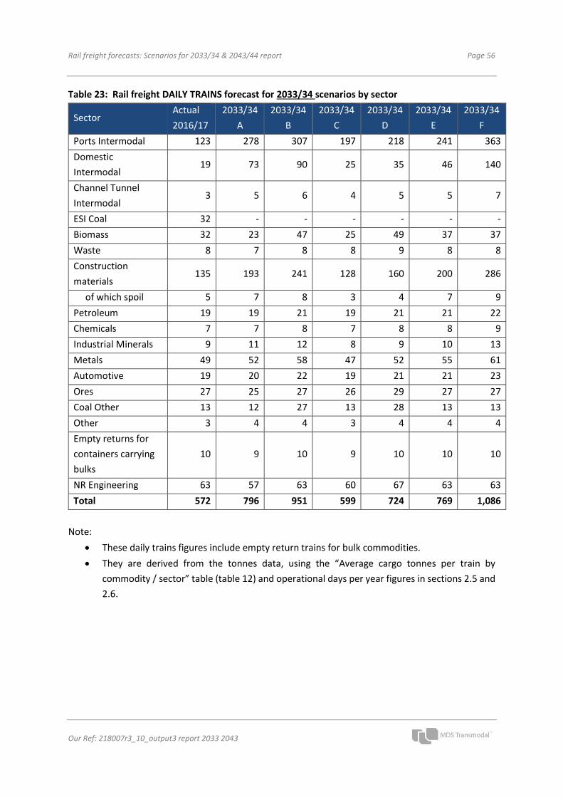
Rail freight forecasts: Scenarios for 2033/34 & 2043/44 report Page 56
Our Ref: 218007r3_10_output3 report 2033 2043
Table 23: Rail freight DAILY TRAINS forecast for 2033/34 scenarios by sector
Sector Actual
2016/17
2033/34
A
2033/34
B
2033/34
C
2033/34
D
2033/34
E
2033/34
F
Ports Intermodal 123 278 307 197 218 241 363
Domestic
Intermodal 19 73 90 25 35 46 140
Channel Tunnel
Intermodal 3 5 6 4 5 5 7
ESI Coal 32 - - - - - -
Biomass 32 23 47 25 49 37 37
Waste 8 7 8 8 9 8 8
Construction
materials 135 193 241 128 160 200 286
of which spoil 5 7 8 3 4 7 9
Petroleum 19 19 21 19 21 21 22
Chemicals 7 7 8 7 8 8 9
Industrial Minerals 9 11 12 8 9 10 13
Metals 49 52 58 47 52 55 61
Automotive 19 20 22 19 21 21 23
Ores 27 25 27 26 29 27 27
Coal Other 13 12 27 13 28 13 13
Other 3 4 4 3 4 4 4
Empty returns for
containers carrying
bulks
10 9 10 9 10 10 10
NR Engineering 63 57 63 60 67 63 63
Total 572 796 951 599 724 769 1,086
Note:
• These daily trains figures include empty return trains for bulk commodities.
• They are derived from the tonnes data, using the “Average cargo tonnes per train by
commodity / sector” table (table 12) and operational days per year figures in sections 2.5 and
2.6.

Rail freight forecasts: Scenarios for 2033/34 & 2043/44 report Page 57
Our Ref: 218007r3_10_output3 report 2033 2043
Table 24: Rail freight DAILY TRAINS forecast for 2043/44 scenarios by sector
Sector Actual
2016/17
2043/44
A
2043/44
B
2043/44
C
2043/44
D
2043/44
E
2043/44
F
Ports Intermodal 123 374 409 266 298 325 466
Domestic
Intermodal 19 121 171 39 68 83 209
Channel Tunnel
Intermodal 3 6 7 5 6 6 8
ESI Coal 32 - - - - - -
Biomass 32 23 47 25 49 37 37
Waste 8 7 8 8 9 8 8
Construction
materials 135 254 384 211 318 297 352
of which spoil 5 8 12 7 10 10 11
Petroleum 19 20 22 20 22 21 22
Chemicals 7 8 9 7 8 8 9
Industrial Minerals 9 11 13 10 11 12 13
Metals 49 55 60 52 57 58 62
Automotive 19 20 22 20 22 21 23
Ores 27 25 27 26 29 27 27
Coal Other 13 12 27 13 28 13 13
Other 3 4 4 3 4 4 4
Empty returns for
containers carrying
bulks
10 9 10 9 10 10 10
NR Engineering 63 57 63 60 67 63 63
Total 572 1,006 1,282 774 1,006 995 1,328
Note:
• These daily trains figures include empty return trains for bulk commodities.
• They are derived from the tonnes data, using the “Average cargo tonnes per train by
commodity / sector” table (table 12) and operational days per year figures in sections 2.5 and
2.6.

Rail freight forecasts: Scenarios for 2033/34 & 2043/44 report Page 58
Our Ref: 218007r3_10_output3 report 2033 2043
Figure 10: Rail freight DAILY TRAINS forecast for 2023/24 scenarios by sector
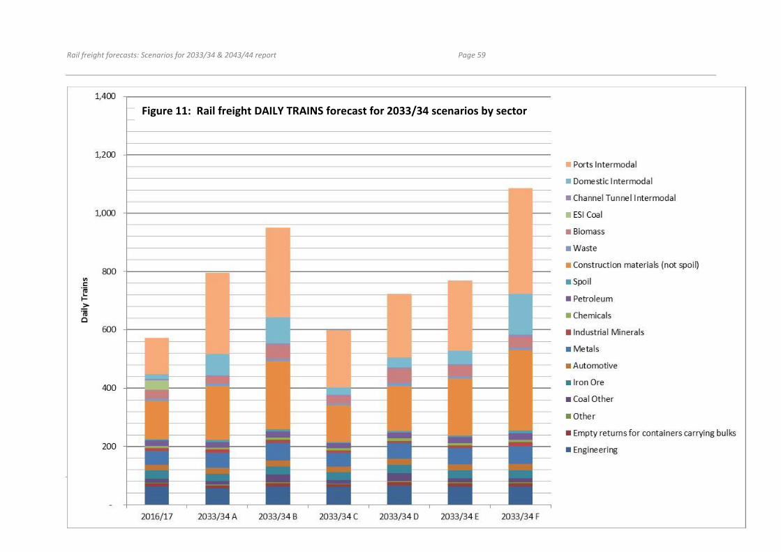
Rail freight forecasts: Scenarios for 2033/34 & 2043/44 report Page 59
Our Ref: 218007r3_10_output3 report 2033 2043
Figure 11: Rail freight DAILY TRAINS forecast for 2033/34 scenarios by sector

Rail freight forecasts: Scenarios for 2033/34 & 2043/44 report Page 60
Our Ref: 218007r3_10_output3 report 2033 2043
Figure 12: Rail freight DAILY TRAINS forecast for 2043/44 scenarios by sector

Rail freight forecasts: Scenarios for 2033/34 & 2043/44 report Page 61
Our Ref: 218007r3_10_output3 report 2033 2043
Table 25: Rail freight HOURLY PATHS forecast for 2023/24 scenarios by sector
Sector 2016/17 2023/24 A2 2023/24 B2 2023/24 C2 2023/24 D2
Ports Intermodal 8.0 11.4 12.8 7.6 8.5
Domestic Intermodal 1.2 3.8 4.1 1.6 1.7
Channel Tunnel Intermodal 0.2 0.2 0.3 0.2 0.2
ESI Coal 3.9 - - - -
Biomass 2.4 2.9 4.5 3.1 4.8
Waste 0.9 0.8 0.9 0.9 1.0
Construction materials 20.1 26.2 34.3 19.0 24.9
of which spoil 0.5 0.7 0.9 0.5 0.7
Petroleum 1.9 1.9 2.1 1.8 2.0
Chemicals 0.8 0.8 0.9 0.8 0.9
Industrial Minerals 1.0 1.1 1.3 0.9 1.0
Metals 5.3 5.6 6.1 4.9 5.5
Automotive 2.1 2.1 2.6 2.0 2.6
Ores 3.0 2.7 3.0 2.9 3.2
Coal Other 1.7 1.5 3.3 1.6 3.5
Other 0.4 0.4 0.4 0.3 0.4
Empty returns for
containers carrying bulks 1.1 1.0 1.1 1.0 1.2
NR Engineering 3.5 3.2 3.5 3.3 3.7
Total 57.6 65.7 81.1 52.0 64.7
Note:
• These hourly path figures are derived from the daily trains data, using the “Path utilisation by
commodity / sector” table and the 18 hours per day figure in section 2.6.

Rail freight forecasts: Scenarios for 2033/34 & 2043/44 report Page 62
Our Ref: 218007r3_10_output3 report 2033 2043
Table 26: Rail freight HOURLY PATHS forecast for 2033/34 scenarios by sector
Sector Actual
2016/17
2033/34
A
2033/34
B
2033/34
C
2033/34
D
2033/34
E
2033/34
F
Ports Intermodal 8.0 18.2 20.1 12.8 14.3 15.7 23.7
Domestic
Intermodal 1.2 4.8 5.9 1.6 2.3 3.0 9.1
Channel Tunnel
Intermodal 0.2 0.3 0.4 0.3 0.3 0.3 0.5
ESI Coal 3.9 - - - - - -
Biomass 2.4 1.7 3.5 1.8 3.7 2.7 2.7
Waste 0.9 0.8 0.9 0.9 1.0 0.9 0.9
Construction
materials 20.1 28.7 35.9 19.1 23.9 29.8 42.5
of which spoil 0.5 0.7 0.9 0.4 0.5 0.8 1.0
Petroleum 1.9 1.9 2.1 1.9 2.1 2.0 2.2
Chemicals 0.8 0.8 0.9 0.8 0.9 0.9 1.0
Industrial Minerals 1.0 1.2 1.3 0.9 1.0 1.1 1.4
Metals 5.3 5.7 6.3 5.2 5.7 6.0 6.6
Automotive 2.1 2.2 2.4 2.2 2.4 2.3 2.6
Ores 3.0 2.7 3.0 2.9 3.2 3.0 3.0
Coal Other 1.7 1.5 3.3 1.6 3.5 1.7 1.7
Other 0.4 0.4 0.5 0.4 0.4 0.4 0.4
Empty returns for
containers carrying
bulks
1.1 1.0 1.1 1.1 1.2 1.1 1.1
NR Engineering 3.5 3.2 3.5 3.3 3.7 3.5 3.5
Total 57.6 75.1 91.0 56.6 69.2 74.5 103.0
Note:
• These hourly path figures are derived from the daily trains data, using the “Path utilisation by
commodity / sector” table and the 18 hours per day figure in section 2.6.

Rail freight forecasts: Scenarios for 2033/34 & 2043/44 report Page 63
Our Ref: 218007r3_10_output3 report 2033 2043
Table 27: Rail freight HOURLY PATHS forecast for 2043/44 scenarios by sector
Sector Actual
2016/17
2043/44
A
2043/44
B
2043/44
C
2043/44
D
2043/44
E
2043/44
F
Ports Intermodal 8.0 24.5 26.7 17.4 19.5 21.2 30.5
Domestic
Intermodal 1.2 7.9 11.2 2.6 4.5 5.4 13.7
Channel Tunnel
Intermodal 0.2 0.4 0.4 0.3 0.4 0.4 0.5
ESI Coal 3.9 - - - - - -
Biomass 2.4 1.7 3.5 1.8 3.7 2.7 2.7
Waste 0.9 0.8 0.9 0.9 1.0 0.9 0.9
Construction
materials 20.1 37.9 57.2 31.3 47.4 44.3 52.4
of which spoil 0.5 0.9 1.4 0.8 1.1 1.1 1.2
Petroleum 1.9 2.0 2.2 2.0 2.2 2.1 2.2
Chemicals 0.8 0.9 1.0 0.8 0.9 0.9 1.0
Industrial Minerals 1.0 1.3 1.4 1.1 1.2 1.3 1.4
Metals 5.3 5.9 6.6 5.6 6.2 6.3 6.7
Automotive 2.1 2.2 2.5 2.2 2.5 2.4 2.6
Ores 3.0 2.7 3.0 2.9 3.2 3.0 3.0
Coal Other 1.7 1.5 3.3 1.6 3.5 1.7 1.7
Other 0.4 0.4 0.5 0.4 0.4 0.4 0.4
Empty returns for
containers carrying
bulks
1.1 1.0 1.1 1.1 1.2 1.1 1.1
NR Engineering 3.5 3.2 3.5 3.3 3.7 3.5 3.5
Total 57.6 94.3 124.9 75.3 101.2 97.7 124.5
Note:
• These hourly path figures are derived from the daily trains data, using the “Path utilisation by
commodity / sector” table and the 18 hours per day figure in section 2.6.

Rail freight forecasts: Scenarios for 2033/34 & 2043/44 report Page 64
Our Ref: 218007r3_10_output3 report 2033 2043
Figure 13: Rail freight HOURLY PATHS forecast for 2023/24 scenarios by sector
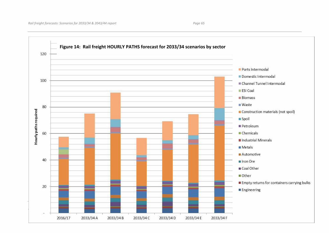
Rail freight forecasts: Scenarios for 2033/34 & 2043/44 report Page 65
Our Ref: 218007r3_10_output3 report 2033 2043
Figure 14: Rail freight HOURLY PATHS forecast for 2033/34 scenarios by sector

Rail freight forecasts: Scenarios for 2033/34 & 2043/44 report Page 66
Our Ref: 218007r3_10_output3 report 2033 2043
Figure 15: Rail freight HOURLY PATHS forecast for 2043/44 scenarios by sector

Rail freight forecasts: Scenarios for 2033/34 & 2043/44 report Page 67
Our Ref: 218007r3_10_output3 report 2033 2043
4.3 Comparison with Freight Market Study (FMS) The table and graph below shows how the new 2023/24, 2033/34 and 2043/44 scenarios compare
with the FMS forecasts, along with the historical traffics from 2004/05. It also shows what the FMS
forecasts would have been for 2016/17 if out-turn assumptions for 2016/17 had been input into the
FMS models.
Table 28: Comparison of new forecasts with the FMS
Scenario Million Tonnes
2016/17 actual 85.8
2023/24 A2: Factors favouring rail, low market growth 104.6
2023/24 B2: Factors favouring rail, high market growth 128.2
2023/24 C2: Factors disfavouring rail, low market growth 78.4
2023/24 D2: Factors disfavouring rail, high market growth 97.1
2023/24 Average of A2, B2, C2 & D2 102.0
2023/24 A3: A2 with capacity constraint 101.5
2023/24 B3: B2 with capacity constraint 119.7
2033/34 A: Factors favouring rail, low market growth 121.2
2033/34 B: Factors favouring rail, high market growth 147.0
2033/34 C: Factors disfavouring rail, low market growth 86.3
2033/34 D: Factors disfavouring rail, high market growth 106.3
2033/34 E: Central 113.1
2033/34 F: Internalisation of external costs 159.1
2043/44 A: Factors favouring rail, low market growth 153.6
2043/44 B: Factors favouring rail, high market growth 200.2
2043/44 C: Factors disfavouring rail, low market growth 113.5
2043/44 D: Factors disfavouring rail, high market growth 151.1
2043/44 E: Central 147.7
2043/44 F: Internalisation of external costs 194.3
2012 actual (from FMS) (12 months to the end of September 2012) 112.4
2016/17 forecast from FMS base with 2016/17 assumptions 77.1
Original FMS central case forecast for 2023/24 127.0
Original FMS central case forecast for 2033/34 161.1
Original FMS central case forecast for 2043/44 211.7

Rail freight forecasts: Scenarios for 2033/34 & 2043/44 report Page 68
Our Ref: 218007r3_10_output3 report 2033 2043
Figure 16
Note the “FMS-based forecast of 2016/17” line shows what a forecast of 2016/17 would have been
(77 m tonnes) using
• the FMS base year (12 months to the end of September 2012)
• input assumptions that reflect the true outcome in 2016/17 (such as lower fuel prices)
• the forecasting methods used in the FMS
See our May 2018 report on 2023/24 forecasts for further details.
ESI (power station) coal has historically been a volatile commodity – and is no longer forecast to be
carried by rail in these forecast scenarios. The graph below shows an equivalent graph but with ESI
coal excluded. Note that the graph does include biomass, which reflects conversion of power stations
from coal to biomass.

Rail freight forecasts: Scenarios for 2033/34 & 2043/44 report Page 69
Our Ref: 218007r3_10_output3 report 2033 2043
Figure 17
The FMS forecasts of 2013 were at the top end of the range of our new forecasts. Our new forecasts
show:
• Lower growth in intermodal traffics due to the less favourable revised input assumptions for
rail costs versus road costs (particularly lower fuel costs), and a lower extent to which we
assume rail-served distribution parks will be developed.
• Lower biomass growth (the FMS had 14m tonnes)
• Higher construction materials growth due to a larger assumed growth in the overall market
than previously forecast in the FMS

Rail freight forecasts: Scenarios for 2033/34 & 2043/44 report Page 70
Our Ref: 218007r3_10_output3 report 2033 2043
5. COMMENTARY ON FORECAST RESULTS
The results from the modelling of the 6 2033/34 and 2043/44 capacity-unconstrained scenarios
demonstrate that differences in exogenous circumstances have a large effect on the rail freight
industry. If the factors that favour rail come to pass with high market growth (scenario B), there will
be overall significant growth of 133% by 2043/44, but if the factors that disfavour rail come to pass
with low market growth (scenario C), there will be only an overall slight increase in rail freight tonnage
of 1% to 2033/34 and of 32% to 2043/44. Unsurprisingly the result for the high market growth
scenarios (scenarios B & D) show larger traffic volumes than their respective low market growth
scenarios (scenarios A & C).
5.1 Coal & Biomass ESI coal is eliminated as per the defined assumptions. Some of the large increases in “coal other” and
biomass in scenarios B & D are due to commodity-specific defined input assumptions:
• growth at Drax with Lynemouth coming on-stream
• and the new planned coal flow from Cumbria to East Coast ports in Northern England.
5.2 Construction materials Construction materials also had a defined assumption about market growth in the high-market-
growth scenarios (in line with GDP: up 68.7% to 2043/44). However more than half of the construction
materials growth in scenario B is due to the rail mode share increases resulting from the rail-favouring
assumptions (increased fuel and wage costs and slightly longer trains).
In scenario C (disfavouring rail and low market growth) in 2033/34, the model results suggest that rail
would lose some of its construction materials traffic due to the significant increase in variable track
access charges (+130%). When producing results, the model implicitly assumes that a market
equilibrium has been reached. However the present-day reality is that the industry is buying wagons
and investing in infrastructure on the expectation of growth, and that track charges will probably not
significantly increase further to this extent. This gives some stability to the market. Another factor
not included in the modelling is that several super-quarries have planning restrictions on their road
freight volumes, thus limiting the scope to which they could easily switch mode to road. Both of these
factors suggest that if the assumptions in scenario C were to come to pass, the slight decline that the
model suggests may not materialise in the real world.
Higher variable access charges in 2033/34 partly explain why there is a fall in construction materials
volumes between 2023/24 and 2033/34 under scenario D (see tables 16 and 17). Another factor is

Rail freight forecasts: Scenarios for 2033/34 & 2043/44 report Page 71
Our Ref: 218007r3_10_output3 report 2033 2043
that the uplift which was applied to the 2023/24 forecasts to reflect the impact of major infrastructure
schemes was not applied in 2033/34 (or 2043/44).
5.3 Intermodal Ports intermodal shows large growth for scenarios A & B due to the inland rail-served warehousing,
high trade growth, increased fuel and wage costs, slightly longer trains and retention of MSRS grants.
For scenario C, despite lower trade growth (+35% in 2033/34), lower fuel price growth, lower HGV
drivers’ wage growth, no change in train length, and removing MSRS, traffic is still up 60% (equivalent
to 2.8% per year), helped by inland rail-served warehousing and increased fuel and wage costs.
The huge potential market for domestic non-bulk traffic is currently largely untapped by rail, starting
from a very low base. Domestic intermodal follows a similar pattern to ports intermodal but is
particularly boosted by the building of rail-served warehousing which removes the need for a local
road haul between warehouse and terminal. The market can easily switch between road and rail and
is highly price sensitive as shown by the large difference between the scenarios in 2043/44: +110% in
scenario C and +1000% in scenario F where rail is particularly boosted by the charging of externalities
to road and rail.
As with the construction sector, there may be some inertia in the intermodal market, with the industry
taking some time to adjust, such that growth may take a few years to catch up with the potential
traffic that the modelling suggests is available, particularly for scenarios A, B and F.
Scenario F is built on the central forecast (scenario E), with extra transport costs representing the
internalisation of external costs. Following our MSB-based approach (see section 2.4), these extra
costs would increase road costs much more than rail costs. This encourages further mode switch from
road to rail: an extra 32% of total rail tonnes in 2043/44. For those highly elastic commodities which
can easily switch between road and rail (such as intermodal containers), there is a larger switch to rail
with an additional 65%.
5.4 Other commodities The forecasts for sectors such as metals, ores and petroleum are relatively stable under all scenarios,
compared with those for intermodal and construction materials, for example. This reflects the
assumptions used for these scenarios as noted above (e.g. no major changes in the overall markets or
modest (5%) reductions or increases). It is recognised that it is a possibility that some of these sectors
may experience larger falls in overall markets, due to factors such as further declines in the steel
industry (for the metals and ores sectors) and electrification / decarbonisation of road transport (for
the petroleum sector). This, in turn, could lead to larger falls in these sectors than under scenarios A
and C, for example. While this represents a downside risk for the forecasts, there is also an upside

Rail freight forecasts: Scenarios for 2033/34 & 2043/44 report Page 72
Our Ref: 218007r3_10_output3 report 2033 2043
risk that the forecasts are too low because they do not include any forecasts for new markets – see
below.
5.5 Potential new markets There is concern about local air pollution, climate change and congestion on the roads, along with
economic drivers such as increased fuel costs and drivers’ wages making road more expensive. In this
environment, there may be further opportunities for rail freight growth away from the traditional
sectors.
With the combined socio-economic trends toward urban repopulation, same-day delivery and urban
convenience grocery retail formats, demand for delivery of consumer goods into urban areas is
growing. In parallel, concerns over urban air quality and road congestion are challenging established
means of distribution; so too the loss of legacy urban distribution space to the very residential
development fuelling population growth. Against such a backdrop promoters believe there is an
opportunity for the development of a rail haul offer for consignments of consumer goods directly into
urban centres for onward distribution by zero-carbon delivery vehicles.
Under such a scenario, lighter weight, higher speed (which on some routes would make pathing them
amongst passenger trains easier), shuttle frequency freights services could link established national
distribution facilities directly into urban logistics hubs developed on the railway estate or potentially
exploit out of hours opportunities at major passenger termini.
Our existing freight model is not currently configured to forecast this sector, so this potential new
market is not quantified in this report. However there may be scope to undertake some quantified
modelling and analysis in future.

Rail freight forecasts: Scenarios for 2033/34 & 2043/44 report Page 73
Our Ref: 218007r3_10_output3 report 2033 2043
6. ASSIGNMENTS TO THE RAIL NETWORK
It can be easier to visualise the impact of these forecasts by assigning the base year and forecast traffic
to the rail network. It is often more meaningful to describe the number of freight trains on each route,
rather than the tonnage. In terms of capacity and timetabling, the number of hourly paths required
on each route is often the most useful means of quantifying rail freight demand.
All freight trains using the network are assigned to the network for each of the 365 days separately in
the base year 2016/17. For each individual train, the traffic is scaled up in line with the origin to
destination by commodity tonnage forecasts. This ensures that for each train, the routing and the
tonnes per train are maintained in the forecasts (i.e. base year routings are assumed to continue). In
scenarios A & B, all base year traffics are subject to the 5% increased tonnage per train, so the number
of trains required to carry the same cargo is scaled by 1.0/1.05.
The maps show the routes that the trains actually take in the base year; primary routes as well as
timetabled secondary and diversionary routes. For example for trains from Southampton to the West
Midlands and beyond, the main route is via Winchester with many trains, and the main diversionary
route is via Laverstock junctions with just a handful of trains. For all commodities (excluding additional
intermodal), because the base year assignments include the diversionary routes, these same
diversionary routes are included in the forecasts.
The exception to this is for forecast additional intermodal traffic, because this is often to/from new
sites for which there are no base year trains to scale up. For intermodal trains, the current average
cargo tonnage per train is 507 tonnes.
By default routes for additional intermodal traffic are assumed to be along the shortest path between
origin and destination sites, along a route with a loading gauge of at least W8 – for example Felixstowe
to the West Midlands and North West is via Peterborough and Nuneaton, not London. Diversionary
routes are not considered. However for various terminal to terminal flows, we have stipulated specific
en-route ‘via-points’, to ensure that those routes are more realistic – with a preference for W10
routes; Additional intermodal traffic on the ECML is routed along the GN/GE route via Lincoln.
No active re-routings have been considered. For example existing trains on the East Coast Main Line
(ECML) have NOT been diverted to the GN/GE route via Lincoln and existing trains using cross-London
routes have NOT been diverted to the cross-country Felixstowe to Nuneaton route. We have not
taken account of planned schemes such as East West Rail.
As the assignments are unconstrained forecasts of demand, the routings for all trains do not take into
account any future timetabling / capacity issues etc. There is therefore the potential to re-route some
of these forecast freight trains onto less congested routes where appropriate.

Rail freight forecasts: Scenarios for 2033/34 & 2043/44 report Page 74
Our Ref: 218007r3_10_output3 report 2033 2043
Once a freight train assignment has been made for each day in the base year and each forecast
scenario and year, they can be averaged to give a daily average for each year. There are fewer freight
trains on Saturdays, Sundays and on bank holidays, so to give a more representative picture of the
typical weekday traffic volumes, all Saturdays, Sundays and bank holidays are discarded when
calculating the daily average.
In the raw train movement data, each train route travelled is recorded as a series of en-route ‘via-
points’ including the origin and destination. The network does not yet include every origin and
destination location (Stanox) code in the network. Therefore some trains do not appear to start at
the correct location on their branch line, and only appear at the first recognised junction. For example
trains from Peak Forest Cemex in Derbyshire appear to start at Chinley East junction. The assignment
maps are therefore best suited to quantifying traffic on main lines rather than branch lines.
Figures 18, 19 and 20 show daily trains (sum of both directions) for
• 2016/17
• 2033/34 scenario E (Central forecast)
• 2043/44 scenario E (Central forecast)
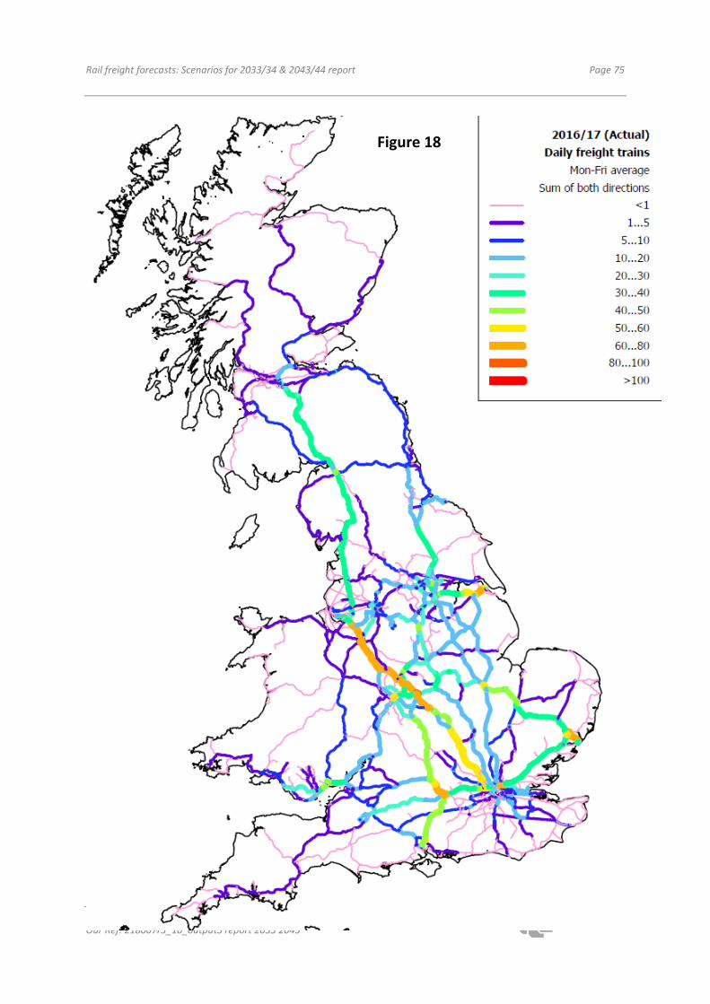
Rail freight forecasts: Scenarios for 2033/34 & 2043/44 report Page 75
Our Ref: 218007r3_10_output3 report 2033 2043
Figure 18

Rail freight forecasts: Scenarios for 2033/34 & 2043/44 report Page 76
Our Ref: 218007r3_10_output3 report 2033 2043
Figure 19

Rail freight forecasts: Scenarios for 2033/34 & 2043/44 report Page 77
Our Ref: 218007r3_10_output3 report 2033 2043
Figure 20

Rail freight forecasts: Scenarios for 2033/34 & 2043/44 report Page 78
Our Ref: 218007r3_10_output3 report 2033 2043
7. RAIL MARKET SHARES
In the base year (2016/17) there were 1.4 billion tonnes lifted and 148 billion tonne kms by road
(source: DfT’s Continuing Survey of Road Goods Transport (CSRGT)10). Therefore the base year rail
mode share is 5.7% by tonnes and 11% by tonne kms.
Road traffic data for individual commodities / sectors is not always available in a consistent way to
enable a direct comparison of road versus rail traffics. For example it is difficult to precisely define a
road equivalent for rail’s “domestic intermodal”, and road data does not distinguish between ESI
(power station) coal and “other coal”.
However an indication of the road traffic and therefore rail’s mode shares is given below for each
rail sector. For the base year this is based on the rail data and the DfT’s CSRGT. For 2023/24,
2033/34 and 2043/44, the road data is scaled up/down using the sectoral market growths described
in the assumptions.
Table 29: 2016/17. Million tonnes by road and rail by sector, and rail mode shares
Sector Rail Road Total Rail mode share Notes
Automotive 0.4 39.0 39.4 1.1%
Biomass 6.5 19.0 25.5 25% 1
Chemicals 0.9 47.0 47.9 1.9%
Coal Other 2.0 6.0 8.0 25% 2
Construction materials (inc spoil) 24.3 323.0 347.3 7.0%
Empty returns for containers carrying bulks 0.4 0.0 0.4 100% 3
NR Engineering 6.7 0.0 6.7 100%
ESI Coal 6.3 0.0 6.3 100% 4
Industrial Minerals 1.3 4.0 5.3 25% 5
Channel Tunnel Intermodal 0.4 0.0 0.4 100%
Domestic Intermodal 2.5 652.8 655.3 0.4% 6
Ports Intermodal 16.2 79.2 95.4 17% 7
Ores 4.3 0.0 4.3 100%
Metals 7.4 43.0 50.4 15%
Other 0.3 0.0 0.3 100% 8
Petroleum 4.7 42.0 46.7 10.1%
Waste 1.2 171.0 172.2 0.7%
Grand Total 85.8 1,426 1,512 5.7%
10 In March 2018 the DfT corrected their published CSRGT data from 2011 quarter 2 onwards; which resulted in a reduction of 24% in their reported total tonnes lifted by road in 2016. The revised figures are used in these tables – including correcting the 2023/24 table from the version in our May 2018 report.

Rail freight forecasts: Scenarios for 2033/34 & 2043/44 report Page 79
Our Ref: 218007r3_10_output3 report 2033 2043
Notes:
1. Road tonnes probably includes more than just biomass, so rail's mode share is probably
understated
2. Some road coal may perhaps be to power stations
3. Not easy to find equivalent tonnage in road data
4. Some road coal may perhaps be to power stations, so the true rail share may be slightly lower
than 100%
5. Difficult to define consistently with road data
6. Assumed to be the non-bulk cargoes, although difficult to consistently define for road
7. Road deduced from DfT’s Port Freight Statistics minus transhipment and rail traffic. For Tonne
km mode share, average length of haul for road is calculated based on adjusted CSRGT data
8. Difficult to define consistently
Table 30: Rail mode shares for the base year and 2023/24 scenarios. Tonnes
2023/24
Sector 2016/17 A2 B2 C2 D2 A3 B3
Automotive 1.1% 1.2% 1.4% 1.2% 1.3% 1.2% 1.1%
Biomass 25% 31% 41% 31% 41% 31% 40%
Chemicals 1.9% 2.1% 2.1% 1.9% 1.9% 2.0% 2.0%
Coal Other 25% 25% 39% 25% 39% 25% 39%
Construction materials (inc spoil) 7.0% 9.1% 11% 6.3% 7.6% 8.9% 11%
Empty returns for containers carrying bulks 100% 100% 100% 100% 100% 100% 100%
NR Engineering 100% 100% 100% 100% 100% 100% 100%
ESI Coal 100% 0% 0% 0% 0% 0% 0%
Industrial Minerals 25% 31% 31% 23% 23% 31% 31%
Channel Tunnel Intermodal 100% 100% 100% 100% 100% 100% 100%
Domestic Intermodal 0.4% 1.2% 1.2% 0.5% 0.5% 1.1% 1.1%
Ports Intermodal 17% 23% 23% 15% 15% 21% 19%
Ores 100% 100% 100% 100% 100% 100% 100%
Metals 15% 17% 17% 15% 15% 17% 17%
Other 100% 100% 100% 100% 100% 100% 100%
Petroleum 10% 11% 11% 10% 10% 11% 11%
Waste 0.7% 0.7% 0.7% 0.7% 0.7% 0.7% 0.7%
Grand Total 5.7% 6.7% 7.5% 5.1% 5.7% 6.5% 7.0%
Note: For derivation of 2016/17 figures, see table 29.

Rail freight forecasts: Scenarios for 2033/34 & 2043/44 report Page 80
Our Ref: 218007r3_10_output3 report 2033 2043
Table 31: Rail mode shares for the base year and 2033/34 scenarios. Tonnes
2033/34
Sector 2016/17 A B C D E F
Automotive 1.1% 1.3% 1.3% 1.2% 1.2% 1.2% 1.4%
Biomass 25% 21% 35% 21% 35% 28% 28%
Chemicals 1.9% 2.1% 2.1% 1.9% 1.9% 2.0% 2.3%
Coal Other 25% 25% 39% 25% 39% 25% 25%
Construction materials (inc spoil) 7.0% 9.7% 9.7% 6.1% 6.1% 8.5% 12.1%
Empty returns for containers carrying bulks 100% 100% 100% 100% 100% 100% 100%
NR Engineering 100% 100% 100% 100% 100% 100% 100%
ESI Coal 100% 0% 0% 0% 0% 0% 0%
Industrial Minerals 25% 32% 32% 23% 23% 28% 35%
Channel Tunnel Intermodal 100% 100% 100% 100% 100% 100% 100%
Domestic Intermodal 0.4% 1.4% 1.4% 0.5% 0.5% 0.8% 2.3%
Ports Intermodal 17% 30% 29% 20% 19% 23% 35%
Ores 100% 100% 100% 100% 100% 100% 100%
Metals 15% 18% 18% 15% 15% 17% 18%
Other 100% 100% 100% 100% 100% 100% 100%
Petroleum 10% 11% 11% 10% 10% 11% 12%
Waste 0.7% 0.7% 0.7% 0.7% 0.7% 0.7% 0.7%
Grand Total 5.7% 7.5% 7.6% 5.4% 5.5% 6.4% 9.0%
Note: For derivation of 2016/17 figures, see table 29

Rail freight forecasts: Scenarios for 2033/34 & 2043/44 report Page 81
Our Ref: 218007r3_10_output3 report 2033 2043
Table 32: Rail mode shares for the base year and 2043/44 scenarios. Tonnes
2043/44
Sector 2016/17 A B C D E F
Automotive 1.1% 1.3% 1.3% 1.3% 1.3% 1.3% 1.4%
Biomass 25% 21% 35% 21% 35% 28% 28%
Chemicals 1.9% 2.2% 2.2% 2.0% 2.0% 2.1% 2.3%
Coal Other 25% 25% 39% 25% 39% 25% 25%
Construction materials (inc spoil) 7.0% 12% 12% 10% 10% 11% 13%
Empty returns for containers carrying bulks 100% 100% 100% 100% 100% 100% 100%
NR Engineering 100% 100% 100% 100% 100% 100% 100%
ESI Coal 100% 0% 0% 0% 0% 0% 0%
Industrial Minerals 25% 35% 35% 29% 29% 32% 36%
Channel Tunnel Intermodal 100% 100% 100% 100% 100% 100% 100%
Domestic Intermodal 0.4% 2.3% 2.1% 0.7% 0.8% 1.2% 3.0%
Ports Intermodal 17% 34% 33% 23% 23% 26% 38%
Ores 100% 100% 100% 100% 100% 100% 100%
Metals 15% 18% 18% 17% 17% 18% 19%
Other 100% 100% 100% 100% 100% 100% 100%
Petroleum 10% 11% 11% 11% 11% 11% 12%
Waste 0.7% 0.7% 0.7% 0.7% 0.7% 0.7% 0.7%
Grand Total 5.7% 9.2% 8.7% 6.8% 6.6% 7.4% 9.8%
Note: For derivation of 2016/17 figures, see table 29

Rail freight forecasts: Scenarios for 2033/34 & 2043/44 report Page 82
Our Ref: 218007r3_10_output3 report 2033 2043
Table 33: 2016/17. Billion tonne kilometres by road and rail by sector, and rail mode shares
Sector Rail Road Total Rail mode share
Automotive 0.1 5.2 5.3 2.7%
Biomass 0.9 2.1 3.0 29%
Chemicals 0.1 6.4 6.5 2.2%
Coal Other 0.3 0.6 0.9 31%
Construction materials (inc spoil) 4.3 21.6 25.9 17%
Empty returns for containers carrying bulks 0.1 0.0 0.1 100%
NR Engineering 1.7 0.0 1.7 100%
ESI Coal 1.2 0.0 1.2 100%
Industrial Minerals 0.2 0.3 0.6 41%
Channel Tunnel Intermodal 0.1 0.0 0.1 100%
Domestic Intermodal 1.1 75.6 76.8 1.5%
Ports Intermodal 5.6 15.7 21.4 26%
Ores 0.2 0.0 0.2 100%
Metals 1.6 5.1 6.7 24%
Other 0.1 0.0 0.1 100%
Petroleum 1.1 4.0 5.1 22%
Waste 0.2 10.9 11.1 1.9%
Grand Total 19.0 147.5 166.5 11%
See notes to above table “2016/17. Million tonnes by road and rail by sector, and rail mode shares”

Rail freight forecasts: Scenarios for 2033/34 & 2043/44 report Page 83
Our Ref: 218007r3_10_output3 report 2033 2043
Table 34: Rail mode shares for the base year and 2023/24 scenarios. Tonne Kilometres
2023/24
Sector 2016/17 A2 B2 C2 D2 A3 B3
Automotive 2.7% 2.9% 3.2% 2.8% 3.1% 2.7% 2.6%
Biomass 29% 34% 45% 34% 45% 34% 44%
Chemicals 2.2% 2.4% 2.4% 2.2% 2.2% 2.4% 2.3%
Coal Other 31% 31% 69% 31% 69% 31% 69%
Construction materials (inc spoil) 17% 19% 23% 15% 18% 19% 22%
Empty returns for containers carrying bulks 100% 100% 100% 100% 100% 100% 100%
NR Engineering 100% 100% 100% 100% 100% 100% 100%
ESI Coal 100% 0% 0% 0% 0% 0% 0%
Industrial Minerals 41% 48% 48% 39% 39% 48% 47%
Channel Tunnel Intermodal 100% 100% 100% 100% 100% 100% 100%
Domestic Intermodal 1.5% 4.3% 4.3% 1.9% 1.9% 4.2% 4.0%
Ports Intermodal 26% 35% 35% 23% 23% 32% 28%
Ores 100% 100% 100% 100% 100% 100% 100%
Metals 24% 27% 27% 23% 23% 27% 27%
Other 100% 100% 100% 100% 100% 100% 100%
Petroleum 22% 24% 24% 22% 22% 24% 24%
Waste 1.9% 1.9% 1.9% 1.9% 1.9% 1.9% 1.9%
Grand Total 11% 14% 15% 10% 11% 13% 14%
Note: For derivation of 2016/17 figures, see table 33

Rail freight forecasts: Scenarios for 2033/34 & 2043/44 report Page 84
Our Ref: 218007r3_10_output3 report 2033 2043
Table 35: Rail mode shares for the base year and 2033/34 scenarios. Tonne Kilometres
2033/34
Sector 2016/17 A B C D E F
Automotive 2.7% 3.0% 3.0% 2.9% 2.9% 2.9% 3.3%
Biomass 29% 23% 38% 23% 38% 31% 31%
Chemicals 2.2% 2.5% 2.5% 2.2% 2.2% 2.4% 2.7%
Coal Other 31% 31% 69% 31% 69% 31% 31%
Construction materials (inc spoil) 17% 20% 20% 14% 14% 18% 23%
Empty returns for containers carrying bulks 100% 100% 100% 100% 100% 100% 100%
NR Engineering 100% 100% 100% 100% 100% 100% 100%
ESI Coal 100% 0% 0% 0% 0% 0% 0%
Industrial Minerals 41% 50% 50% 40% 40% 46% 53%
Channel Tunnel Intermodal 100% 100% 100% 100% 100% 100% 100%
Domestic Intermodal 1.5% 4.9% 5.0% 1.7% 1.8% 2.7% 9.0%
Ports Intermodal 26% 51% 49% 34% 34% 40% 59%
Ores 100% 100% 100% 100% 100% 100% 100%
Metals 24% 28% 28% 23% 23% 26% 28%
Other 100% 100% 100% 100% 100% 100% 100%
Petroleum 22% 24% 24% 23% 23% 23% 25%
Waste 1.9% 1.9% 1.9% 1.9% 1.9% 1.9% 1.9%
Grand Total 11% 17% 17% 12% 12% 14% 21%
Note: For derivation of 2016/17 figures, see table 33

Rail freight forecasts: Scenarios for 2033/34 & 2043/44 report Page 85
Our Ref: 218007r3_10_output3 report 2033 2043
Table 36: Rail mode shares for the base year and 2043/44 scenarios. Tonne Kilometres
2043/44
Sector 2016/17 A B C D E F
Automotive 2.7% 3.1% 3.1% 3.0% 3.0% 3.0% 3.3%
Biomass 29% 23% 38% 23% 38% 31% 31%
Chemicals 2.2% 2.6% 2.6% 2.4% 2.4% 2.5% 2.7%
Coal Other 31% 31% 69% 31% 69% 31% 31%
Construction materials (inc spoil) 17% 23% 23% 18% 18% 21% 24%
Empty returns for containers carrying bulks 100% 100% 100% 100% 100% 100% 100%
NR Engineering 100% 100% 100% 100% 100% 100% 100%
ESI Coal 100% 0% 0% 0% 0% 0% 0%
Industrial Minerals 41% 56% 56% 47% 47% 51% 56%
Channel Tunnel Intermodal 100% 100% 100% 100% 100% 100% 100%
Domestic Intermodal 1.5% 7.4% 7.4% 2.5% 2.9% 4.2% 11.1%
Ports Intermodal 26% 57% 56% 40% 41% 46% 64%
Ores 100% 100% 100% 100% 100% 100% 100%
Metals 24% 29% 29% 25% 25% 27% 29%
Other 100% 100% 100% 100% 100% 100% 100%
Petroleum 22% 24% 24% 23% 23% 24% 25%
Waste 1.9% 1.9% 1.9% 1.9% 1.9% 1.9% 1.9%
Grand Total 11% 21% 20% 15% 14% 17% 24%
Note: For derivation of 2016/17 figures, see table 33

Rail freight forecasts: Scenarios for 2033/34 & 2043/44 report Page 86
Our Ref: 218007r3_10_output3 report 2033 2043
8. SENSITIVITY TEST G: A “EUROPEAN GAUGE” FREIGHT ROUTE
“European gauge” is taken to be a sufficiently generous loading gauge that would allow larger wagons
to be carried including “Piggyback”: HGV trailers on rail wagons – which cannot normally be
accommodated on the British rail network.
We have tested an indicative concept of a European gauge route rather than a specific new route,
connecting the end of the Channel Tunnel Rail Link (CTRL) in East London via North London, the East
Midlands, South Yorkshire, Southwest Manchester, Carlisle and Glasgow, linking to Thames and
Humber ports.
Being a dedicated freight route potentially means that longer, heavier trains could be carried, with a
faster end-to-end journey time because they would not need to wait in passing loops for timetabled
slots between passenger trains on the classic network. Rail unit costs would be reduced because
assets would be used more intensively.
This route would have the capacity to cater for likely demand. This additional capacity would be for
the benefit of both freight trains using the route and for passenger trains because there would be
fewer freight trains to have to share the existing routes with.
We have tested four distinct markets for a potential European gauge freight route – building on the
2043/44 high market growth, favouring rail scenario (scenario B):
• International piggyback (HGV trailers on rail wagons) through the Channel tunnel and to/from
ports (Thames and Humber). These are modelled as equivalent to inland extensions of
unaccompanied ferry services to/from the continent – to inland terminals in East London,
West London, Leicestershire, South Yorkshire, Greater Manchester and the Scottish Central
Belt
• Domestic piggyback - directly diverting HGVs off the road network. These are modelled with
just the HGV trailers carried by rail: i.e. not the HGV cab with driver, because this would
involve the weight of the cab being carried around unnecessarily, and the driver’s time during
transit. This is similar to existing intermodal rail services where there needs to be a local road
haul at each end to transfer the cargo from the original origin to the origin rail terminal, and
then from the destination rail terminal to the final destination.
• Rail journeys that operate solely on the freight route with the opportunity for longer, heavier,
higher-gauge trains. This was modelled by assuming 50% longer trains (instead of 5% longer)
and 80kph instead of 50kph average speeds.
• Existing non-Piggyback Channel Tunnel type services but with longer, heavier, higher-gauge
trains. As above, this was modelled by assuming 50% longer trains (instead of 5% longer) and
80kph instead of 50kph average speeds

Rail freight forecasts: Scenarios for 2033/34 & 2043/44 report Page 87
Our Ref: 218007r3_10_output3 report 2033 2043
The various markets are forecast to attract the following tonnes:
Table 37: European gauge freight route potential market. Thousand tonnes per year
Sector Thousand Tonnes
Piggyback Humber ports 4,990
Piggyback Thames ports 4,297
Piggyback Channel Tunnel 1,036
Piggyback Domestic 8,880
Non-Piggyback Channel Tunnel 4,079
Solely on freight route 10,210
Total 33,492
If we were to assume the current average cargo tonnes per train (577 tonnes), along with 260
operational days per year, and an average of 18 operational hours per day (see sections 2.5 & 2.6),
this annual tonnage would equate to 223 trains per day or 12 trains per hour on the route. However
these train counts would probably be slightly lower because of the potential for higher tonnes per
train along the route meaning slightly fewer trains are required to carry the same tonnage.
The availability of these new transport offerings to the market would detract from “classic” rail’s
market – reducing it by 11.7 million tonnes. The net additional rail freight traffic would therefore be
21.8 million tonnes per year.
Some “classic” rail freight traffic is also likely to divert onto the route for part of its journey. Because
some of its journey would be on the classic network, the trains would not be able to be longer, heavier,
higher-gauge trains, so there would be unlikely to be significant user cost savings. However the
principal benefit of switching these trains to the freight route may be to relieve capacity.

Rail freight forecasts: Scenarios for 2033/34 & 2043/44 report Page 88
Our Ref: 218007r3_10_output3 report 2033 2043
9. CONCLUSION
This report describes rail freight forecast demand results for 4 different 2023/24 scenarios (taken from
our May 2018 report on 2023/24 forecasts), 6 2033/34 scenarios and 6 2043/44 scenarios spanning
factors favouring rail to factors disfavouring rail, and low market growth to high market growth with
scenario F representing internalisation of external costs. These are presented in terms of tonnes,
tonne kms, daily trains and hourly paths required. Sensitivity test G (European gauge freight route) is
also presented.
The rail-favouring scenarios (A, B and F) show significant growth in demand across the network.
However in reality there are likely to be capacity constraints at some locations. We have not
conducted any capacity constraint for 2033/34 and 2043/44 for this study.
ESI (power station) coal has historically been a volatile commodity – and is no longer forecast to be
carried by rail in these forecast scenarios. The graph below show how the new scenarios compare
with the FMS forecasts, along with the historical traffics from 2004/05 but with ESI coal excluded.

Rail freight forecasts: Scenarios for 2033/34 & 2043/44 report Page 89
Our Ref: 218007r3_10_output3 report 2033 2043
Figure 21
The FMS forecasts of 2013 were at the top end of the range of our new forecasts. Our new forecasts
show:
• Lower growth in intermodal traffics due to the less favourable revised input assumptions for
rail costs versus road costs, and a lower extent to which we assume rail-served distribution
parks will be developed.
• Lower biomass growth (the FMS had 14m tonnes)
• Higher construction materials growth due to a larger assumed growth in the overall market
than previously forecast
The report describes the assumptions and methods for the various sectors, along with a market share
analysis.
These forecasts demonstrate that differences in exogenous circumstances can have a large impact on
the rail freight industry, with the total 2043/44 forecast rail freight tonnage ranging from 114 million
tonnes in scenario C to 200 million tonnes in scenario B. Scenario E (central scenario) results in 148
million tonnes in 2043/44. This is equivalent to a 2.0% growth per year from 2016/17, or a 2.3%
growth per year if ESI coal is excluded.

Rail freight forecasts: Scenarios for 2033/34 & 2043/44 report Page 90
Our Ref: 218007r3_10_output3 report 2033 2043
Fuel prices in particular impact on rail’s ability to compete with road – with high fuel prices adversely
affecting road more than rail, thus encouraging a switch from road to rail. Drivers’ wages are also
important, as is the development of rail-served warehousing for domestic intermodal traffic.
It should be noted that the model implicitly includes the assumption that the market will have fully
adapted to the market conditions input into the model. However in the real world, many of the
investments in assets are long-term – which gives the rail freight sector some inertia. The market is
therefore unlikely to have fully adapted to very different conditions over a 7 year period to 2023/24,
although in the longer term, if the market players foresee the changes we have assumed (such as
increased availability of rail served warehousing sites, higher fuel and drivers’ wage costs) and believe
that rail capacity will be available to justify the necessary investments, the market should be able to
adapt in the long term.