radioss theory manual - altair hyperworks · radioss theory manual 11.0 version – jan 2011 large...
TRANSCRIPT
RADIOSS THEORY MANUAL 11.0 version – Jan 2011
Large Displacement Finite Element Analysis Chapter 5
Altair Engineering, Inc., World Headquarters: 1820 E. Big Beaver Rd., Troy MI 48083-2031 USA Phone: +1.248.614.2400 • Fax: +1.248.614.2411 • www.altair.com • [email protected]
RADIOSS THEORY Version 11.0 CONTENTS
30-Jan-2011 1
CONTENTS 5.1 SOLID HEXAHEDRON ELEMENTS 5
5.1.1 SHAPE FUNCTIONS FOR LINEAR BRICKS 5 5.1.2 STRAIN RATE 7 5.1.3 ASSUMED STRAIN RATE 7 5.1.4 INTERNAL FORCE CALCULATION 9 5.1.5 HOURGLASS MODES 10 5.1.6 STABILITY 14 5.1.7 SHOCK WAVES 15 5.1.8 ELEMENT DEGENERATION 15 5.1.9 INTERNAL STRESS CALCULATION 17 5.1.10 DEVIATORIC STRESS CALCULATION 20
5.2 SOLID TETRAHEDRON ELEMENTS 23 5.2.1 4 NODE SOLID TETRAHEDRON 23 5.2.2 10 NODE SOLID TETRAHEDRON 23
5.3 SHELL ELEMENTS 27 5.3.1 INTRODUCTION 27 5.3.2 BILINEAR MINDLIN PLATE ELEMENT 28 5.3.3 TIME STEP FOR STABILITY 29 5.3.4 LOCAL REFERENCE FRAME 29 5.3.5 BILINEAR SHAPE FUNCTIONS 30 5.3.6 MECHANICAL PROPERTIES 31 5.3.7 INTERNAL FORCES 34 5.3.8 HOURGLASS MODES 35 5.3.9 HOURGLASS RESISTANCE 37 5.3.10 STRESS AND STRAIN CALCULATION 41 5.3.11 CALCULATION OF FORCES AND MOMENTS 48 5.3.12 QPH, QPPS, QEPH AND QBAT SHELL FORMULATIONS 51 5.3.12.1 FORMULATIONS FOR A GENERAL DEGENERATED 4-NODE SHELL 51 5.3.12.2 FULLY-INTEGRATED SHELL ELEMENT QBAT 54 5.3.12.3 THE NEW ONE-POINT QUADRATURE SHELL ELEMENT 55 5.3.12.4 ADVANCED ELASTO-PLASTIC HOURGLASS CONTROL 60 5.3.13 THREE-NODE SHELL ELEMENTS 61 5.3.14 COMPOSITE SHELL ELEMENTS 65 5.3.14.1 TRANSFORMATION MATRIX FROM GLOBAL TO ORTHOTROPIC SKEW 65 5.3.14.2 COMPOSITE MODELING IN RADIOSS 66 5.3.14.3 ELEMENT ORIENTATION 66 5.3.14.4 ORTHOTROPIC SHELLS 68 5.3.14.5 COMPOSITE SHELL 68 5.3.14.6 COMPOSITE SHELL WITH VARIABLE LAYERS 69 5.3.14.7 LIMITATIONS 69 5.3.15 THREE-NODE TRIANGLE WITHOUT ROTATIONAL D.O.F. (SH3N6) 69 5.3.15.1 STRAIN COMPUTATION 70 5.3.15.2 BOUNDARY CONDITIONS APPLICATION 72
5.4 SOLID-SHELL ELEMENTS 74 5.5 TRUSS ELEMENTS (TYPE 2) 77
5.5.1 PROPERTY INPUT 77 5.5.2 STABILITY 77 5.5.3 RIGID BODY MOTION 77 5.5.4 STRAIN 78 5.5.5 MATERIAL TYPE 78 5.5.6 FORCE CALCULATION 78
5.6 BEAM ELEMENTS (TYPE 3) 79 5.6.1 LOCAL COORDINATE SYSTEM 79 5.6.2 BEAM ELEMENT GEOMETRY 79
RADIOSS THEORY Version 11.0 CONTENTS
30-Jan-2011 2
5.6.3 MINIMUM TIME STEP 80 5.6.4 BEAM ELEMENT BEHAVIOR 80 5.6.5 MATERIAL PROPERTIES 83 5.6.6 INERTIA COMPUTATION 85
5.7 ONE DEGREE OF FREEDOM SPRING ELEMENTS (TYPE 4) 86 5.7.1 TIME STEP 87 5.7.2 LINEAR SPRING 87 5.7.3 NONLINEAR ELASTIC SPRING 88 5.7.4 NONLINEAR ELASTO-PLASTIC SPRING - ISOTROPIC HARDENING 89 5.7.5 NONLINEAR ELASTO-PLASTIC SPRING - DECOUPLED HARDENING 90 5.7.6 NONLINEAR ELASTIC-PLASTIC SPRING - KINEMATIC HARDENING 90 5.7.7 NONLINEAR ELASTO-PLASTIC SPRING - NON LINEAR UNLOADING 91 5.7.8 NONLINEAR DASHPOT 91 5.7.9 NONLINEAR VISCOELASTIC SPRING 92
5.8 GENERAL SPRING ELEMENTS (TYPE 8) 94 5.8.1 TIME STEP 94 5.8.2 LINEAR SPRING 94 5.8.3 NONLINEAR ELASTIC SPRING 94 5.8.4 NONLINEAR ELASTO-PLASTIC SPRING - ISOTROPIC HARDENING 94 5.8.5 NONLINEAR ELASTO-PLASTIC SPRING - DECOUPLED HARDENING 94 5.8.6 NONLINEAR ELASTO-PLASTIC SPRING - KINEMATIC HARDENING 94 5.8.7 NONLINEAR ELASTO-PLASTIC SPRING - NON LINEAR UNLOADING 94 5.8.8 NONLINEAR DASHPOT 94 5.8.9 NONLINEAR VISCOELASTIC SPRING 94 5.8.10 SKEW FRAME PROPERTIES 94 5.8.11 DEFORMATION SIGN CONVENTION 96 5.8.12 TRANSLATIONAL FORCES 96 5.8.13 MOMENTS 97 5.8.14 MULTIDIRECTIONAL FAILURE CRITERIA 98
5.9 PULLEY TYPE SPRING ELEMENTS (TYPE 12) 99 5.9.1 TIME STEP 99 5.9.2 LINEAR SPRING 99 5.9.3 NONLINEAR ELASTIC SPRING 99 5.9.4 NONLINEAR ELASTO-PLASTIC SPRING - ISOTROPIC HARDENING 99 5.9.5 NONLINEAR ELASTO-PLASTIC SPRING - DECOUPLED HARDENING 100 5.9.6 NONLINEAR DASHPOT 100 5.9.7 NONLINEAR VISCO-ELASTIC SPRING 100 5.9.8 FRICTION EFFECTS 100
5.10 BEAM TYPE SPRING ELEMENTS (TYPE 13) 102 5.10.1 TIME STEP 102 5.10.2 LINEAR SPRING 103 5.10.3 NONLINEAR ELASTIC SPRING 103 5.10.4 NONLINEAR ELASTO-PLASTIC SPRING - ISOTROPIC HARDENING 103 5.10.5 NONLINEAR ELASTO-PLASTIC SPRING - DECOUPLED HARDENING 103 5.10.6 NONLINEAR ELASTO-PLASTIC SPRING - KINEMATIC HARDENING 103 5.10.7 NONLINEAR ELASTO-PLASTIC SPRING - NON LINEAR UNLOADING 103 5.10.8 NONLINEAR DASHPOT 103 5.10.9 NONLINEAR VISCO-ELASTIC SPRING 103 5.10.10 SKEW FRAME PROPERTIES 103 5.10.11 SIGN CONVENTIONS 104 5.10.12 TENSION 104 5.10.13 SHEAR - XY 105 5.10.14 SHEAR - XZ 106 5.10.15 TORSION 107 5.10.16 BENDING ABOUT THE Y AXIS 107 5.10.17 BENDING ABOUT THE Z AXIS 107 5.10.18 MULTIDIRECTIONAL FAILURE CRITERIA 108

RADIOSS THEORY Version 11.0 CONTENTS
30-Jan-2011 3
5.11 MULTISTRAND ELEMENTS (TYPE 28) 109 5.11.1 INTRODUCING MULTISTRAND ELEMENTS 109 5.11.2 INTERNAL FORCES COMPUTATION 109
5.12 SPRING TYPE PRETENSIONER (TYPE 32) 112 5.12.1 INTRODUCING PRETENSIONERS 112 5.12.2 RADIOSS MODEL FOR PRETENSIONERS 112

30-Jan-2011 4
ELEMENT LIBRARY
Chapter
RADIOSS THEORY Version 11.0 ELEMENT LIBRARY
30-Jan-2011 5
5.0 ELEMENT LIBRARY RADIOSS element library contains elements for one, two or three dimensional problems. Some new elements have been developed and implemented in recent versions. Most of them use the assumed strain method to avoid some locking problems. For the elements using reduced integration schema, the physical stabilization method is used to control efficiently the hourglass deformations. Another point in these new elements is the use of co-rotational coordinate system. For the new solid elements, as the assumed strains are often defined in the specific directions, the use of global system combined with Jaumman's stress derivation contributes to commutative error especially when solid undergoes large shear strains. The RADIOSS finite element library can be classified into the following categories of elements:
• Solid elements : 8- and 20-node bricks, 4- and 10-node tetrahedrons,
• Solid-shells : 8- , 16- and 20-node hexahedrons, 6-node pentahedral element,
• 2 dimensional elements : 4-node quadrilaterals for plane strain and axisymmetrical analysis,
• Shell elements : 4-node quadrilaterals and 3-node triangles,
• One dimensional elements: rivet, springs, bar and beams.
The implementation of these elements will now be detailed. Expression of nodal forces will be developed as, for explicit codes they represent the discretization of the momentum equations. Stiffness matrices, which are central to implicit finite element approaches, are not developed here.
5.1 Solid Hexahedron Elements RADIOSS brick elements have the following properties:
• BRICK8: 8-node linear element with reduced or full integration,
• HA8: 8-node linear element with various number of integration points going from 2x2x2 to 9x9x9,
• HEPH: 8-node linear element with reduced integration point and physical stabilization of hourglass modes,
• BRICK20: 20-node quadratic element with reduced or full integration schemes.
For all elements, a lumped mass approach is used and the elements are isoparametric, i.e. the same shape functions are used to define element geometry and element displacements
The fundamental theory of each element is described in this chapter.
5.1.1 Shape functions for linear bricks Shape functions define the geometry of an element in its computational (intrinsic) domain. As was seen in Chapter 3, physical coordinates are transformed into simpler computational intrinsic coordinates so that integration of values is numerically more efficient.

RADIOSS THEORY Version 11.0 ELEMENT LIBRARY
30-Jan-2011 6
Figure 5.1.1 8 Node Brick Element
Where: ξ≡r , η≡s , ζ≡t
The shape functions of an 8 node brick element, shown in Figure 5.1.1, are given by:
( )( )( )ζηξ −−−=Φ 11181
1 EQ. 5.1.1.1
( )( )( )ζηξ +−−=Φ 11181
2 EQ. 5.1.1.2
( )( )( )ζηξ +−+=Φ 11181
3 EQ. 5.1.1.3
( )( )( )ζηξ −−+=Φ 11181
4 EQ. 5.1.1.4
( )( )( )ζηξ −+−=Φ 11181
5 EQ. 5.1.1.5
( )( )( )ζηξ ++−=Φ 11181
6 EQ. 5.1.1.6
( )( )( )ζηξ +++=Φ 11181
7 EQ. 5.1.1.7
( )( )( )ζηξ −++=Φ 11181
8 EQ. 5.1.1.8
The element velocity field is related by:
iII
Ii vv .8
1∑
=
Φ= EQ. 5.1.1.9
where the iIv are the nodal velocities.

RADIOSS THEORY Version 11.0 ELEMENT LIBRARY
30-Jan-2011 7
5.1.2 Strain rate The relationship between the physical coordinate and computational intrinsic coordinates system for a brick element is given by the matrix equation:
⎥⎥⎥⎥⎥⎥
⎦
⎤
⎢⎢⎢⎢⎢⎢
⎣
⎡
∂Φ∂∂Φ∂∂Φ∂
=
⎥⎥⎥⎥⎥⎥
⎦
⎤
⎢⎢⎢⎢⎢⎢
⎣
⎡
∂Φ∂∂Φ∂∂Φ∂
⎥⎥⎥⎥⎥⎥⎥
⎦
⎤
⎢⎢⎢⎢⎢⎢⎢
⎣
⎡
∂∂
∂∂
∂∂
∂∂
∂∂
∂∂
∂∂
∂∂
∂∂
=
⎥⎥⎥⎥⎥⎥⎥
⎦
⎤
⎢⎢⎢⎢⎢⎢⎢
⎣
⎡
∂Φ∂∂Φ∂∂Φ∂
z
y
xF
z
y
x
zyx
zyx
zyx
I
I
I
I
I
I
I
I
I
.. ξ
ζζζ
ηηη
ξξξ
ζ
η
ξ
EQ. 5.1.2.1
Hence:
⎥⎦
⎤⎢⎣
⎡∂Φ∂
=⎥⎦
⎤⎢⎣
⎡∂Φ∂ −
ξξI
i
I Fx
.1 EQ. 5.1.2.2
where ξF is the Jacobian matrix.
The element strain rate is defined as:
⎟⎟⎠
⎞⎜⎜⎝
⎛
∂
∂+
∂∂
=i
j
j
iij x
vxv
21ε& EQ. 5.1.2.3
Relating the element velocity field to its shape function gives:
iII j
I
j
i vxx
v⋅
∂Φ∂
=∂∂ ∑
=
8
1 EQ. 5.1.2.4
Hence, the strain rate can be described directly in terms of the shape function:
iII j
I
i
j
j
iij v
xxv
xv
⋅∂Φ∂
=⎟⎟⎠
⎞⎜⎜⎝
⎛
∂
∂+
∂∂
= ∑=
8
121ε& EQ. 5.1.2.5
As was seen in section 2.4.1, volumetric strain rate is calculated separately by volume variation.
For one integration point:
jjjjjjjj xxxxxxxx ∂
Φ∂−=
∂Φ∂
∂Φ∂
−=∂Φ∂
∂Φ∂
−=∂Φ∂
∂Φ∂
−=∂Φ∂ 64538271 ;;; EQ. 5.1.2.6
F.E Method is used only for deviatoric strain rate calculation in A.L.E and Euler formulation.
Volumetric strain rate is computed separately by transport of density and volume variation.
5.1.3 Assumed strain rate Using Voigt convention, the strain rate of EQ. 5.1.2.5 can be written as:
{ } [ ]{ } [ ]{ }∑=
==8
1III vBvBε& EQ. 5.1.3.1

RADIOSS THEORY Version 11.0 ELEMENT LIBRARY
30-Jan-2011 8
With,
{ } t
xzyzxyzzyyxx εεεεεεε &&&&&&& 222=
[ ]
t
III
III
III
I
zyz
zxy
yxx
B
⎥⎥⎥⎥⎥⎥⎥
⎦
⎤
⎢⎢⎢⎢⎢⎢⎢
⎣
⎡
∂Φ∂
∂Φ∂
∂Φ∂
∂Φ∂
∂Φ∂
∂Φ∂
∂Φ∂
∂Φ∂
∂Φ∂
=
000
000
000
It is useful to take the Belytschko-Bachrach's mix form [27] of the shape functions written by:
( ) ∑=
+⋅+⋅+⋅+Δ=Φ4
1
,,,,,α
ααφγζηξ IzIyIxIII zbybxbzyx EQ. 5.1.3.2
Where,
( )
ξηζξηξζηζφ
γ
ζηξ
ααααα
=
⎥⎦
⎤⎢⎣
⎡⎟⎠
⎞⎜⎝
⎛Γ−⎟
⎠
⎞⎜⎝
⎛Γ−⎟
⎠
⎞⎜⎝
⎛Γ−Γ=
===∂Φ∂
=
∑∑∑===
;81
;0
8
1
8
1
8
1zI
JJJyI
JJJxI
JJJII
i
IiI
bzbybx
xb
The derivation of the shape functions is given by:
∑=
∂∂+=
∂Φ∂ 4
1α
φα αγixIiI
i
I bx
EQ. 5.1.3.3
It is decomposed by a constant part which is directly formulated with the Cartesian coordinates, and a non-constant part which is to be approached separately. For the strain rate, only the non-constant part is modified by the assumed strain. We can see in following that the non-constant part or the high order part is just the hourglass terms.
We have now the decomposition of the strain rate:
{ } [ ]{ } [ ] [ ]( ){ } { } { }H
II
HII
III vBBvB εεε &&& +=+== ∑∑
==
08
1
08
1 EQ. 5.1.3.4
with:
[ ]
⎥⎥⎥⎥⎥⎥⎥⎥
⎦
⎤
⎢⎢⎢⎢⎢⎢⎢⎢
⎣
⎡
=
yxIzI
xIzI
xIyxI
zI
yxI
xI
I
bbbb
bbb
bb
B
00
000
0000
0 ; [ ]
t
zIyIzI
zIxIyI
yIxIxI
HIB
⎥⎥⎥⎥⎥⎥⎥
⎦
⎤
⎢⎢⎢⎢⎢⎢⎢
⎣
⎡
=
∑∑∑
∑∑∑
∑∑∑
=∂
∂
=∂
∂
=∂
∂
=∂
∂
=∂
∂
=∂
∂
=∂
∂
=∂
∂
=∂
∂
000
000
000
4
1
4
1
4
1
4
1
4
1
4
1
4
1
4
1
4
1
α
φα
α
φα
α
φα
α
φα
α
φα
α
φα
α
φα
α
φα
α
φα
ααα
ααα
ααα
γγγ
γγγ
γγγ

RADIOSS THEORY Version 11.0 ELEMENT LIBRARY
30-Jan-2011 9
Belvtschko and Bindeman [65] ASQBI assumed strain is used:
{ } [ ] [ ]( ){ }∑=
+=8
1
0
II
HII vBBε& EQ. 5.1.3.5
with
[ ]
⎥⎥⎥⎥⎥⎥⎥⎥
⎦
⎤
⎢⎢⎢⎢⎢⎢⎢⎢
⎣
⎡
−−−−−−−−−−−−
=
2323
1313
1212
1234241142
3411234143
3422431234
00
0
II
II
II
IIIII
IIIII
IIIII
HI
YZXZ
XYZYYXX
ZZYXXZZYYX
B νννννννννννν
where xIxIIX ∂∂
∂∂ += 31 3113 φφ γγ ; yIyIIY ∂
∂∂∂ += 31 3113 φφ γγ ; ;1 ν
νν −=
To avoid shear locking, some hourglass modes are eliminated in the terms associated with shear so that no shear strain occurs during pure bending. E.g.: 33 , II XY in xyε& terms and all fourth hourglass modes in shear terms are
also removed since this mode is non-physical and is stabilized by other terms in [ ]HIB .
The terms with Poisson coefficient are added to obtain an isochoric assumed strain field when the nodal velocity is equivoluminal. This avoids volumetric locking as 5.0=ν . In addition, these terms enable the element to capture transverse strains which occurs in a beam or plate in bending. The plane strain expressions are used since this prevents incompatibility of the velocity associated with the assumed strains.
5.1.3.1 Incompressible or quasi-incompressible cases (Flag for new solid element: Icpr =0,1,2)
For incompressible or quasi- incompressible materials, the new solid elements have no volume locking problem due to the assumed strain. Another way to deal with this problem is to decompose the stress field into the spherical part and the deviatory part and use reduced integration for spherical part so that the pressure is constant. This method has the advantage on the computation time, especially for the full integrated element. For some materials which the incompressibility can be changed during computation (e.g.: elastoplastic material, which becomes incompressible as the growth of plasticity), the treatment is more complicated. Since the elastoplastic material with large strain is the most frequently used, the constant pressure method has been chosen for RADIOSS usual solid elements. The flag Icpr has been introduced for new solid elements.
• Icpr =0: assumed strain with ν terms is used.
• Icpr =1: assumed strain without ν terms and with a constant pressure method is used. The method is recommended for incompressible (initial) materials.
• Icpr =2: assumed strain with ν terms is used, where ν is variable in function of the plasticity state. The formulation is recommended for elastoplastic materials.
5.1.4 Internal force calculation Internal forces are computed using the generalized relation:
Ω∂Φ∂
= ∫Ω
dx
fj
IijiI σint EQ. 5.1.4.1

RADIOSS THEORY Version 11.0 ELEMENT LIBRARY
30-Jan-2011 10
However, to increase the computational speed of the process, some simplifications are applied.
5.1.4.1 Reduced Integration Method This is the default method for computing internal forces. A one point integration scheme with constant stress in the element is used. Due to the nature of the shape functions, the amount of computation can be substantially reduced:
jjjjjjjj xxxxxxxx ∂Φ∂
−=∂Φ∂
∂Φ∂
−=∂Φ∂
∂Φ∂
−=∂Φ∂
∂Φ∂
−=∂Φ∂ 64538271 ;;; EQ. 5.1.4.2
Hence, the value j
I
x∂Φ∂
is taken at the integration point and the internal force is computed using the relation:
Ω⎟⎟⎠
⎞⎜⎜⎝
⎛
∂Φ∂
=0j
IijiI x
F σ EQ. 5.1.4.3
The force calculation is exact for the special case of the element being a parallelepiped.
5.1.4.2 Full Integration Method The final approach that can be used is the full generalized formulation found in EQ. 5.1.4.1. A classical eight point integration scheme, with non-constant stress, but constant pressure is used to avoid locking problems. This is computationally expensive, having eight deviatoric stress tensors, but will produce accurate results with no hourglass.
When assumed strains are used with full integration (HA8 element), the reduced integration of pressure is no more necessary, as the assumed strain is then a free locking problem.
5.1.4.3 Improved Integration Method for ALE This is an ALE method for computing internal forces (flag INTEG). A constant stress in the element is used.
The value ∫Ω
Ω∂Φ∂ dx j
I is computed with Gauss points.
5.1.5 Hourglass modes Hourglass modes are element distortions that have zero strain energy. Thus, no stresses are created within the element. There are 12 hourglass modes for a brick element, 4 modes for each of the 3 coordinate directions. Γ represents the hourglass mode vector, as defined by Flanagan-Belytschko [12]. They produce linear strain modes, which cannot be accounted for using a standard one point integration scheme.
( )1,1,1,1,1,1,1,11 −+−+−+−+=Γ

RADIOSS THEORY Version 11.0 ELEMENT LIBRARY
30-Jan-2011 11
( )1,1,1,1,1,1,1,12 ++−−−−++=Γ
( )1,1,1,1,1,1,1,13 −++−+−−+=Γ
( )1,1,1,1,1,1,1,14 +−+−−+−+=Γ
To correct this phenomenon, it is necessary to introduce anti-hourglass forces and moments. Two possible formulations are presented hereafter.
5.1.5.1 Kosloff & Frasier Formulation [10] The Kosloff-Frasier hourglass formulation uses a simplified hourglass vector. The hourglass velocity rates are defined as:
∑=
⋅Γ=∂
∂ 8
1IiII
i vt
q αα
EQ. 5.1.5.1
where:
• Γ is the non-orthogonal hourglass mode shape vector,
• ν is the node velocity vector,
• i is the direction index, running from 1 to 3,
• I is the node index, from 1 to 8,
• α is the hourglass mode index, from 1 to 4.
This vector is not perfectly orthogonal to the rigid body and deformation modes.
All hourglass formulations except the physical stabilization formulation for solid elements in RADIOSS use a viscous damping technique. This allows the hourglass resisting forces to be given by:
( ) ∑ Γ⋅∂
∂Ω=
α
αα
ρ Iihgr
iI tqchf
23
41
EQ. 5.1.5.2

RADIOSS THEORY Version 11.0 ELEMENT LIBRARY
30-Jan-2011 12
where:
• ρ is the material density,
• c is the sound speed,
• h is a dimensional scaling coefficient defined in the input,
• Ω is the volume.
5.1.5.2 Flanagan-Belytschko Formulation [12] In the Kosloff-Frasier formulation seen in section 5.1.5.1, the hourglass base vector α
IΓ is not perfectly orthogonal to the rigid body and deformation modes that are taken into account by the one point integration scheme. The mean stress/strain formulation of a one point integration scheme only considers a fully linear velocity field, so that the physical element modes generally contribute to the hourglass energy. To avoid this, the idea in the Flanagan-Belytschko formulation is to build an hourglass velocity field which always remains orthogonal to the physical element modes. This can be written as:
LiniIiI
HouriI vvv −= EQ. 5.1.5.3
The linear portion of the velocity field can be expanded to give:
( )⎟⎟⎠
⎞⎜⎜⎝
⎛−⋅
∂∂
+−= jjj
iIiIiI
HouriI xx
xvvvv EQ. 5.1.5.4
Decomposition on the hourglass vectors base gives [12]:
ααα
Ijj
iliI
HouriII
i xxvvv
tq
Γ⋅⎟⎟⎠
⎞⎜⎜⎝
⎛⋅
∂∂
−=⋅Γ=∂
∂ EQ. 5.1.5.5
where:
tqi
∂∂ α
are the hourglass modal velocities,
αIΓ is the hourglass vectors base.
Remembering that iJj
j
j
i vxx
v⋅
∂
Φ∂=
∂∂
and factorizing EQ. 5.1.5.5 gives:
⎟⎟⎠
⎞⎜⎜⎝
⎛Γ
∂
Φ∂−Γ⋅=
∂∂ αα
α
Ijj
jIiI
i xx
vt
q EQ. 5.1.5.6
αααγ Jjj
jII x
xΓ
∂
Φ∂−Γ= EQ. 5.1.5.7
is the hourglass shape vector used in place of αIΓ in EQ. 5.1.5.2.

RADIOSS THEORY Version 11.0 ELEMENT LIBRARY
30-Jan-2011 13
5.1.5.3 physical hourglass formulation HEPH We try to decompose also the internal force vector as following:
{ } ( ){ } ( ){ }HIII fff int0intint += EQ. 5.1.5.8
In elastic case, we have:
{ } [ ] [ ] [ ]{ }
[ ] [ ]( ) [ ] [ ] [ ]( ){ }∫ ∑
∑∫
Ω =
=Ω
Ω++=
Ω=
dvBBCBB
dvBCBf
j
JHJJ
tHII
j
JJ
t
II
8
1
00
8
1
int
EQ. 5.1.5.9
The constant part ( ){ } [ ]( ) [ ] [ ] { }∫ ∑Ω =
Ω= dvBCBfj
JJ
t
II
8
1
000int is evaluated at the quadrature point just like
other one-point integration formulations mentioned before, and the non-constant part (Hourglass) will be calculated as following:
Taking the simplification of )(;0 jix
j
i ≠=∂∂ξ
(i.e. the Jacobian matrix of EQ. 5.1.2.1 is diagonal), we have:
( ) ∑=
=4
1
int
α
αα γ Ii
HiI Qf EQ. 5.1.5.10
with 12 generalized hourglass stress rates αiQ.
calculated by:
( )[ ]
44
.
.
.
312
11
jiii
ijij
jiiijj
kkik
jjij
iikkjjii
qHQ
qHqHQ
qHqHqHHQ
&
&&
&&&
νμ
νν
μ
μ
+=
⎥⎦⎤
⎢⎣⎡ +
−=
+++=
EQ. 5.1.5.11
and
Ω∂
∂
∂∂
=
Ω⎟⎟⎠
⎞⎜⎜⎝
⎛∂∂
=Ω⎟⎟⎠
⎞⎜⎜⎝
⎛∂∂
=Ω⎟⎟⎠
⎞⎜⎜⎝
⎛∂
∂=
∫
∫∫∫
Ω
ΩΩΩ
dxx
H
dx
dx
dx
H
i
j
j
iij
ii
k
i
jii
φφ
φφφ 2
4
22
3 EQ. 5.1.5.12
Where i,j,k are permuted between 1 to 3 and αiq& has the same definition than in EQ. 5.1.5.6.
Extension to non-linear materials has been done simply by replacing shear modulus μ by its effective tangent values which is evaluated at the quadrature point. For the usual elastoplastic materials, we use a more sophistic procedure which is described in the following section.

RADIOSS THEORY Version 11.0 ELEMENT LIBRARY
30-Jan-2011 14
5.1.5.3.1 Advanced elasto-plastic hourglass control With one-point integration formulation, if the non-constant part follows exactly the state of constant part for the case of elasto-plastic calculation, the plasticity will be under-estimated due to the fact that the constant equivalent stress is often the smallest one in the element and element will be stiffer. Therefore, defining a yield criterion for the non-constant part seems to be a good ideal to overcome this drawback.
Plastic yield criterion:
The von Mises type of criterion is written by:
0),,( 22 =−= yeqf σζηξσ EQ. 5.1.5.13
for any point in the solid element, where yσ is evaluated at the quadrature point.
As only one criterion is used for the non-constant part, two choices are possible:
1. taking the mean value, i.e.: ( ) ΩΩ
== ∫Ω
dff eqeqeq σσσ 1;
2. taking the value by some representative points, e.g. eight Gausse points
The second choice has been used in this element.
Elastro-plastic hourglass stress calculation:
The incremental hourglass stress is computed by:
• Elastic increment
( ) ( ) [ ]{ } tC HHni
trHni Δ+=+ εσσ &1
• Check the yield criterion
• If 0≥f , the hourglass stress correction will be done by un radial return
( ) ( )( )fP trHni
Hni ,11 ++ = σσ
5.1.6 Stability The stability of the numerical algorithm depends on the size of the time step used for time integration (section 4.5). For brick elements, RADIOSS uses the following equation to calculate the size of the time step:
( )12 ++≤
ααclkh EQ. 5.1.6.1
This is the same form as the Courant condition for damped materials. The characteristic length of a particular element is computed using:
SurfaceSideLargestVolumeElementl = EQ. 5.1.6.2
For a 6-sided brick, this length is equal to the smallest distance between two opposite faces.
The terms inside the parentheses in the denominator are specific values for the damping of the material:
• clv
ρα 2
=
• ν effective kinematic viscosity,

RADIOSS THEORY Version 11.0 ELEMENT LIBRARY
30-Jan-2011 15
• ρρ∂
∂=
pc 1 for fluid materials,
• ρ
μλρμ
ρ2
34 +
=+=Kc for a solid elastic material,
• K is the bulk modulus,
• λ , μ are Lame moduli.
The scaling factor k=0.90, is used to prevent strange results that may occur when the time step is equal to the Courant condition. This value can be altered by the user.
5.1.7 Shock waves Shocks are non-isentropic phenomena, i.e. entropy is not conserved, and necessitates a special formulation.
The missing energy is generated by an artificial bulk viscosity q as derived by von Neumann and Richtmeyer [9]. This value is added to the pressure and is computed by:
tlcq
tlqq kk
bkk
a ∂∂
−⎟⎠⎞
⎜⎝⎛
∂∂
=ερερ
222 EQ. 5.1.7.1
where
• l is equal to 3 Ω or to the characteristic length,
• Ω is the volume,
• tkk
∂∂ε
is the volumetric compression strain rate tensor,
• c is the speed of sound in the medium.
The values of aq and bq are adimensional scalar factors defined as:
• aq is a scalar factor on the quadratic viscosity to be adjusted so that the Hugoniot equations are verified. This value is defined by the user. The default value is 1.10.
• bq is a scalar factor on the linear viscosity that damps out the oscillations behind the shock. This is user specified. The default value is 0.05.
Default values are adapted for velocities lower than Mach 2. However for viscoelastic materials (law 34, 35, 38) or honeycomb (law 28), very small values are recommended, i.e. 10-20.
5.1.8 Element degeneration Element degeneration is the collapsing of an element by one or more edges. For example; making an eight node element into a seven node element by giving nodes 7 and 8 the same node number.
The use of degenerated elements for fluid applications is not recommended. The use of degenerated elements for assumed strain formulation is not recommended. If they cannot be avoided, any two nodes belonging to a same edge can be collapsed, with some examples shown below.
For solid elements, it is recommended that element symmetry be maintained.
For 4 node elements, it is recommended that the special tetrahedron element be used.

RADIOSS THEORY Version 11.0 ELEMENT LIBRARY
30-Jan-2011 16
Some examples of element degeneration are shown below.
Not recommended degenerations
Recommended degeneration
Connectivity: 1 2 3 4 5 5 5 5
Connectivity : 1 2 3 4 5 6 6 5

RADIOSS THEORY Version 11.0 ELEMENT LIBRARY
30-Jan-2011 17
5.1.9 Internal stress calculation
5.1.9.1 Global formulation The time integration of stresses has been stated earlier (section 2.6.) as:
( ) ( ) tttt ijijij Δ+=Δ+ σσσ & EQ. 5.1.9.1
The stress rate is comprised of two components: rij
vijij σσσ &&& += EQ. 5.1.9.2
where
• rijσ& is the stress rate due to the rigid body rotational velocity,
• vijσ& is the Jaumann objective stress tensor derivative.
The correction for stress rotation from time t to time t+ tΔ is given by [2]:
kijkkjikrij Ω+Ω= σσσ& EQ. 5.1.9.3
where Ω is the rigid body rotational velocity tensor (EQ. 2.4.1.11).
The Jaumann objective stress tensor derivative vijσ& is the corrected true stress rate tensor without rotational
effects. The constitutive law is directly applied to the Jaumann stress rate tensor.
Deviatoric stresses and pressure (see section 2.7) are computed separately and related by:
ijijij ps δσ −= EQ. 5.1.9.4
where
• ijs is the deviatoric stress tensor;
• p is the pressure or mean stress - defined as positive in compression,
• ijδ is the substitution tensor or unit matrix.
5.1.9.2 Co-rotational Formulation A co-rotational formulation for bricks is a formulation where rigid body rotations are directly computed from the element's node positions. Objective stress and strain tensors are computed in the local (co-rotational) frame. Internal forces are computed in the local frame and then rotated to the global system.
So, when co-rotational formulation is used, EQ. 5.1.10.2 rij
vijij σσσ &&& += reduces to:
vijij σσ && = EQ. 5.1.9.5
where vijσ& is the Jaumann objective stress tensor derivative expressed in the co-rotational frame.
The following illustrates orthogonalization, when one of the r, s, t directions is orthogonal to the two other directions.

RADIOSS THEORY Version 11.0 ELEMENT LIBRARY
30-Jan-2011 18
Isoparametric frames Local (co-rotational) When large rotations occur, this formulation is more accurate than the global formulation, for which the stress rotation due to rigid body rotational velocity is computed in an incremental way.
Co-rotational formulation avoids this kind of problem.
Let us consider the following test:
Z
X
Fix constant velocity on the top of the
The increment of the rigid body rotation vector during time step tΔ is:
( )( )( )⎢
⎢⎢
⎣
⎡
=∂∂−∂∂∂∂=∂∂−∂∂
=∂∂−∂∂
⋅Δ=ΔΩ0//
///
0//
2/yvxv
zvxvzv
xvyv
t
xy
xzx
yx
EQ. 5.1.9.6
So, 2/Ty Δ=ΔΩ α where hv /=α equals the imposed velocity on the top of the brick divided by the height of the brick (constant value).
Due to first order approximation, the increment of stress xxσ due to the rigid body motion is:
( ) xzxzyzxxzyrxx Tτατττσ Δ=ΔΩ=+ΔΩ=Δ 2 EQ. 5.1.9.7
Increment of stress zzσ due to the rigid body motion:
( ) xzxzyzxxzyrzz Tτατττσ Δ−=ΔΩ−=+ΔΩ−=Δ 2 EQ. 5.1.9.8
Increment of shear stress xzτ due to the rigid body motion:
( ) zzzzyxxzzyrxz Tσασσστ Δ=ΔΩ=−ΔΩ=Δ 2 EQ. 5.1.9.9
Increment of shear strain:
( ) TxvzvT zxxz Δ=∂∂+∂∂Δ=Δ αγ // EQ. 5.1.9.10
Increment of stress zzσ due to strain:
0=Δ vzzσ EQ. 5.1.9.11
RADIOSS THEORY Version 11.0 ELEMENT LIBRARY
30-Jan-2011 19
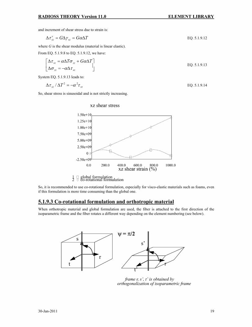
and increment of shear stress due to strain is:
TGG xzvxz Δ=Δ=Δ αγτ EQ. 5.1.9.12
where G is the shear modulus (material is linear elastic).
From EQ. 5.1.9.8 to EQ. 5.1.9.12, we have:
⎥⎦
⎤⎢⎣
⎡Δ−=Δ
Δ+Δ=Δ
xzzz
zzxz TGTτασ
ασατ EQ. 5.1.9.13
System EQ. 5.1.9.13 leads to:
xzxz T τατ 22/ −=ΔΔ EQ. 5.1.9.14
So, shear stress is sinusoidal and is not strictly increasing.
So, it is recommended to use co-rotational formulation, especially for visco-elastic materials such as foams, even if this formulation is more time consuming than the global one.
5.1.9.3 Co-rotational formulation and orthotropic material When orthotropic material and global formulation are used, the fiber is attached to the first direction of the isoparametric frame and the fiber rotates a different way depending on the element numbering (see below).

RADIOSS THEORY Version 11.0 ELEMENT LIBRARY
30-Jan-2011 20
On the other hand, when the co-rotational formulation is used, the orthotropic frame keeps the same orientation with respect to the local (co-rotating) frame, and is therefore also co-rotating (see below).
5.1.10 Deviatoric stress calculation With the stress being separated into deviatoric and pressure (hydrostatic) stress (see section 2.7), it is the deviatoric stress that is responsible for the plastic deformation of the material. The hydrostatic stress will either shrink or expand the volume uniformly, i.e. with proportional change in shape. The determination of the deviatoric stress tensor and whether the material will plastically deform requires a number of steps.
STEP 1: Perform an Elastic Calculation
The deviatoric stress is time integrated from the previous known value using the strain rate to compute an elastic trial stress:
( ) ( ) tGtststts ijkkijrijij
elij Δ⎟
⎠⎞
⎜⎝⎛ −+Δ+=Δ+ δεε &&&
312 EQ. 5.1.10.1
where G is the shear modulus.
This relationship is Hooke's Law, where the strain rate is multiplied by time to give strain.
STEP 2: Compute von Mises Equivalent Stress and Current Yield Stress
Depending on the type of material being modeled, the method by which yielding or failure is determined will vary. The following explanation relates to an elastoplastic material (law 2).
The von Mises equivalent stress relates a three dimensional state of stress back to a simple case of uniaxial tension where material properties for yield and plasticity are well known and easily computed.
The von Mises stress, which is strain rate dependent, is calculated using the equation:
elij
elij
evm ss
23
=σ EQ. 5.1.10.2
The flow stress is calculated from the previous plastic strain:
( ) ( )tbatnp
y εσ += EQ. 5.1.10.3

RADIOSS THEORY Version 11.0 ELEMENT LIBRARY
30-Jan-2011 21
For material types 3, 4, 10, 21, 22, 23 and 36, EQ. 5.1.11.3 is modified according to the different modeling of the material curves.
STEP 3: Plasticity Check
The state of the deformation must be checked.
0≤− yevm σσ
If this equation is satisfied, the state of stress is elastic. Otherwise, the flow stress has been exceeded and a plasticity rule must be used. This is shown in Figure 5.1.2.
Figure 5.1.2 - Plasticity Check
The plasticity algorithm used is due to Mendelson, [1].
STEP 4: Compute Hardening Parameter
The hardening parameter is defined as the slope of the strain-hardening part of the stress-strain curve:
py
dd
Hεσ
= EQ. 5.1.10.4
This is used to compute the plastic strain at time t:
HGt yvmp
+−
=Δ3
σσε& EQ. 5.1.10.5
This plastic strain is time integrated to determine the plastic strain at time tt Δ+ :
( ) ( ) tttt ppp Δ+=Δ+ εεε & EQ. 5.1.10.6
The new flow stress is found using:
( ) ( )ttbattnp
y Δ++=Δ+ εσ EQ. 5.1.10.7
STEP 5: Radial Return
There are many possible methods for obtaining paijs from the trial stress. The most popular method involves a
simple projection to the nearest point on the flow surface, which results in the radial return method.
The radial return calculation is given in EQ. 5.1.10.8. Figure 5.1.3 is a graphic representation of radial return.
elij
vm
ypaij ss
σσ
= EQ. 5.1.10.8

RADIOSS THEORY Version 11.0 ELEMENT LIBRARY
30-Jan-2011 22
Figure 5.1.3 - Radial Return

RADIOSS THEORY Version 11.0 ELEMENT LIBRARY
30-Jan-2011 23
5.2 Solid Tetrahedron Elements
5.2.1 4 node solid tetrahedron The RADIOSS solid tetrahedron element is a 4 node element with one integration point and a linear shape function.
This element has no hourglass. But the drawbacks are the low convergence and the shear locking.
5.2.2 10 node solid tetrahedron The RADIOSS solid tetrahedron element is a 10 nodes element with 4 integration points and a quadratic shape function as shown in Figure 5.2.1.
Figure 5.2.1 – (a) Isoparametric 10 node tetrahedron , (b) Nodal mass distribution
Introducing volume coordinates in an isoparametric frame:
rL =1
sL =2
tL =3
3214 1 LLLL −−−=

RADIOSS THEORY Version 11.0 ELEMENT LIBRARY
30-Jan-2011 24
The shape functions are expressed by:
( ) 111 12 LL −=Φ EQ. 5.2.2.1
( ) 222 12 LL −=Φ EQ. 5.2.2.2
( ) 333 12 LL −=Φ EQ. 5.2.2.3
( ) 444 12 LL −=Φ EQ. 5.2.2.4
215 4 LL=Φ EQ. 5.2.2.5
326 4 LL=Φ EQ. 5.2.2.6
137 4 LL=Φ EQ. 5.2.2.7
418 4 LL=Φ EQ. 5.2.2.8
429 4 LL=Φ EQ. 5.2.2.9
4310 4 LL=Φ EQ. 5.2.2.10
Location of the 4 integration points is expressed by [49].
With,
585410200 ⋅=α and 138196600 ⋅=β
a, b, c, d are the 4 integration points.
5.2.2.1 Advantages and drawbacks This element has various advantages:
• No hourglass
• Compatible with powerful mesh generators
• Fast convergence
• No shear locking.
But there are some drawbacks too:
• Low time step
• Not compatible with ALE formulation
• No direct compatibility with contact interface and other elements.
5.2.2.2 Time step The time step for a regular tetrahedron is computed as:

RADIOSS THEORY Version 11.0 ELEMENT LIBRARY
30-Jan-2011 25
cLdt c= EQ. 5.2.2.11
Where, Lc is the characteristic length of element depending on tetra type. The different types are shown in the following figures:
For a regular 4 node tetra as shown in Figure 5.2.2:
aLaL cc 816.0;32
== EQ. 5.2.2.12
Figure 5.2.2 - 4 nodes tetra
For a regular 10 node tetra as shown in Figure 5.2.3:
aLaL cc 264.0;6
2/5== EQ. 5.2.2.13
Figure 5.2.3 - 10 nodes tetra
For another regular tetra obtained by the assemblage of four hexa as shown in Figure 5.2.4, the characteristic length is:
aLaL cc 204.0;4
3/2== EQ. 5.2.2.14
Figure 5.2.4 - Other regular tetra
5.2.2.3 CPU cost: Time/Element/Cycle The CPU cost is shown in Figure 5.2.5:

RADIOSS THEORY Version 11.0 ELEMENT LIBRARY
30-Jan-2011 26
Figure 5.2.5 - CPU cost in TEC
5.2.2.4 Comparison example Below is a comparison of the 3 types of elements (8-nodes brick, 10-nodes tetra and 20-nodes brick). The results are shown in Figure 5.2.6 for a plastic strain contour.
Figure 5.2.6 - Comparison (plastic strain max = 60%)
8 nodes brick 10 nodes tetras 20 nodes brick8 nodes brick 10 nodes tetras 20 nodes brick

RADIOSS THEORY Version 11.0 ELEMENT LIBRARY
30-Jan-2011 27
5.3 SHELL ELEMENTS Since the degenerated continuum shell element formulation was introduced by Ahmad et al.[38], it has become dominant in commercial Finite Element codes due to its advantage of being independent of any particular shell theory, versatile and cost effective, and applicable in a reliable manner to both thin and thick shells.
In the standard 4-node shell element, full integration and reduced integration schemes have been used to compute the stiffness matrices and force vectors:
- The full integration scheme is often used in programs for static or dynamic problems with implicit time integration. It presents no problem for stability, but sometimes involves “locking” and computations are often more expensive.
- The reduced integration scheme, especially with one-point quadrature (in the mid-surface), is widely used in programs with explicit time integration such as RADIOSS and other programs applied essentially in crashworthiness studies. These elements dramatically decrease the computation time, and are very competitive if the hourglass modes (which result from the reduced integration scheme) are “well” stabilized.
5.3.1 Introduction The historical shell element in RADIOSS is a simple bilinear Mindlin plate element coupled with a reduced integration scheme using one integration point. It is applicable in a reliable manner to both thin and moderately thick shells.
This element is very efficient if the spurious singular modes, called “hourglass modes”, which result from the reduced integration are stabilized.
The stabilization approach consists of providing additional stiffness so that the spurious singular modes are suppressed. Also, it offers the possibility of avoiding some locking problems. One of the first solutions was to generalize the formulation of Kosloff and Frazier [10] for brick element to shell element. It can be shown that the element produces accurate flexural response (thus, free from the membrane shear locking) and is equivalent to the incompatible model element of Wilson et al. [21] without the static condensation procedure. Taylor [47] extended this work to shell elements. Hughes and Liu [22] employed a similar approach and extended it to non linear problems.
Belytschko and Tsay [23] developed a stabilized flat element based on the γ projections developed by Flanagan and Belytschko [12]. Its essential feature is that hourglass control is orthogonal to any linear field, thus preserving consistency. The stabilized stiffness is approached by a diagonal matrix and scaled by the perturbation parameters ih which are introduced as a regulator of the stiffness for nonlinear problems. The
parameters ih are generally chosen to be as small as possible, so this approach is often called a perturbation stabilization.
The elements with perturbation stabilization have two major drawbacks:
• The parameters ih are user-inputs and are generally problem-dependent.
• Poor behavior with irregular geometries (in-plane, out-of-plane). The stabilized stiffness (or stabilized forces) is often evaluated based on a regular flat geometry, so they generally do not pass either the Patch-test or the Twisted beam test.
Belytschko et al. [17] extended this perturbation stabilization to the 4-node shell element which has become widely used in explicit programs.
Belytschko et al. [24] improved the poor behavior exhibited in the warped configuration by adding a coupling curvature-translation term, and a particular nodal projection for the transverse shear calculation analogous to that developed by Hughes and Tezduyar [25], and MacNeal [26]. This element passes the Kirchhoff patch test and the Twisted beam test, but it cannot be extended to a general 6 DOF element due to the particular projection.
Belytschko and Bachrach [27] used a new method called “physical stabilization” to overcome the first drawback of the quadrilateral plane element. This method consists of explicitly evaluating the stabilized stiffness with the help of 'assumed strains', so that no arbitrary parameters need to be prescribed. Engelmann and Whirley [28] have applied it to the 4-node shell element. An alternative way to evaluate the stabilized stiffness explicitly is given by Liu et al. [29] based on Hughes and Liu's 4-node selected reduced integration scheme element [22], in

RADIOSS THEORY Version 11.0 ELEMENT LIBRARY
30-Jan-2011 28
which the strain field is expressed explicitly in terms of natural coordinates by a Taylor-series expansion. A remarkable improvement in the one-point quadrature shell element with physical stabilization has been performed by Belytschko and Leviathan [18]. The element performs superbly for both flat and warped elements especially in linear cases, even in comparison with a similar element under a full integration scheme, and is only 20% slower than the Belytschko and Tsay element. More recently, based on Belytschko and Leviathan's element, Zhu and Zacharia [30] implemented the drilling rotation DOF in their one-point quadrature shell element; the drilling rotation is independently interpolated by the Allman function [39] based on Hughes and Brezzi's [41] mixed variational formulation.
The physical stabilization with assumed strain method seems to offer a rational way of developing a cost effective shell element with a reduced integration scheme. The use of the assumed strains based on the mixed variational principles, is powerful, not only in avoiding the locking problems (volumetric locking, membrane shear locking, as in Belytschko and Bindeman [31]; transverse shear locking, as in Dvorkin and Bathe [32]), but also in providing a new way to compute stiffness. However, as highlighted by Stolarski et al. [33], assumed strain elements generally do not have rigorous foundations; there is almost no constraint for the independent assumed strains interpolation. Therefore, a sound theoretical understanding and numerous tests are needed in order to prove the legitimacy of the assumed strain elements.
The greatest uncertainty of the one-point quadrature shell elements with physical stabilization is with respect to the nonlinear problems. All of these elements with physical stabilization mentioned above rely on the assumptions that the spin and the material properties are constant within the element. The first assumption is necessary to ensure the objectivity principle in geometrical nonlinear problems. The second was adapted in order to extend the explicit evaluation of stabilized stiffness for elastic problems to the physical nonlinear problems. We have found that the second assumption leads to a theoretical contradiction in the case of an elastoplastic problem (a classic physical nonlinear problem), and results in poor behavior in case of certain crash computations.
Zeng and Combescure [15] have proposed an improved 4-node shell element named QPPS with one-point quadrature based on the physical stabilization which is valid for the whole range of its applications (see the Chapter 5.3.12). The formulation is based largely on that of Belytschko and Leviathan.
Based on the QPPS element, Zeng and Winkelmuller have developed a new improved element named QEPH which is integrated in RADIOSS 44 version (see Chapter 5.3.13).
5.3.2 Bilinear Mindlin plate element Most of the following explanation concerns four node plate elements, Figure 5.3.1. Section 5.3.13 explains the three node plate element, shown in Figure 5.3.2.
Figure 5.3.1 - Four Node Plate Element

RADIOSS THEORY Version 11.0 ELEMENT LIBRARY
30-Jan-2011 29
Figure 5.3.2 - Three Node Plate Element
Plate theory assumes that one dimension (the thickness, z) of the structure is small compared to the other dimensions. Hence, the 3D continuum theory is reduced to a 2D theory. Nodal unknowns are the velocities
)( zyx vvv ′′ of the mid plane and the nodal rotation rates ( )yx ωω ′ as a consequence of the suppressed z direction. The thickness of elements can be kept constant, or allowed to be variable. This is user defined. The elements are always in a state of plane stress, i.e. 0=zzσ , or there is no stress acting perpendicular to the plane of the element. A plane orthogonal to the mid-plane remains a plane, but not necessarily orthogonal as in Kirchhoff
theory, (where 0== yzxz εε ) leading to the rotations rates yvz
x ∂∂
−=ω and xvz
y ∂∂
=ω . In Mindlin plate
theory, the rotations are independent variables.
5.3.3 Time step for stability The characteristic length, L, for computing the critical time step, referring back to Figure 5.3.3, is defined by:
( )42,13max1areaL = EQ. 5.3.3.1
( )42,13,41,34,23,12min2 =L EQ. 5.3.3.2
( )21,max LLLc = EQ. 5.3.3.3
When the orthogonalized mode of the hourglass perturbation formulation is used, the characteristic length is defined as:
( )213 ,max LLL = EQ. 5.3.3.4
( )( )fm hh
LLL′
+=
max5.0 21
4 EQ. 5.3.3.5
( )43 ,min LLLc = EQ. 5.3.3.6
where mh is the shell membrane hourglass coefficient and fh is the shell out of plane hourglass coefficient, as mentioned in section 5.3.8.
5.3.4 Local reference frame Three coordinate systems are introduced in the formulation:
• Global Cartesian fixed system ( )kZjYiXXrrr
++=
• Natural system ( )ζηξ ,, , covariant axes x,y
RADIOSS THEORY Version 11.0 ELEMENT LIBRARY
30-Jan-2011 30
• Local systems (x,y,z) defined by an orthogonal set of unit base vectors (t1,t2,n). n is taken to be normal to the mid-surface coinciding with ζ , and (t1,t2 ) are taken in the tangent plane of the mid-surface.
Figure 5.3.3 - Local Reference Frame
The vector normal to the plane of the element at the mid point is defined as:
yxyxn
××
= EQ. 5.3.4.1
The vector defining the local direction is:
xxt =1
yyt =2 EQ. 5.3.4.2
Hence, the vector defining the local direction is found from the cross product of the two previous vectors:
12 tnt ×= EQ. 5.3.4.3
5.3.5 Bilinear shape functions The shape functions defining the bilinear element used in the Mindlin plate are:
( ) ( )( )ηηξξηξ III ++=Φ 1141, EQ. 5.3.5.1
or, in terms of local coordinates:
( ) xydycxbayx IIIII +++=Φ , EQ. 5.3.5.2
It is also useful to write the shape functions in the Belytschko-Bachrach mix form [27]:
( ) ξηγξη IyIxIII ybxbyx +++Δ=Φ ,, EQ. 5.3.5.3
with
( ) ( )[ ] ( )1,1,1,1; =−−=Δ tbytbxtt yII
IxII
III
( ) ( )( )2/;/13423124 jiijxI fffAyyyyb −==
( ) AxxxxbyI /31241342=
( ) ( )[ ] ( )1,1,1,1;4/ −−=ΓΓ−Γ−Γ= xIJ
JxIJ
JII bybxγ
A : area of the element

RADIOSS THEORY Version 11.0 ELEMENT LIBRARY
30-Jan-2011 31
The velocity of the element at the mid-plane reference point is found using the relations:
∑=
Φ=4
1IxIIx vv EQ. 5.3.5.4
∑=
Φ=4
1IyIIy vv EQ. 5.3.5.5
∑=
Φ=4
1IzIIz vv EQ. 5.3.5.6
where, zIyIxI vvv ,, are the nodal velocities in the x,y,z directions.
In a similar fashion, the element rotations are found by:
∑=
Φ=4
1IxIIx ωω EQ. 5.3.5.7
∑=
Φ=4
1IyIIy ωω EQ. 5.3.5.8
where xIω and yIω are the nodal rotational velocities about the x and y reference axes.
The velocity change with respect to the coordinate change is given by:
∑= ∂
Φ∂=
∂∂ 4
1IxI
Ix vxx
v EQ. 5.3.5.9
∑= ∂
Φ∂=
∂∂ 4
1IxI
Ix vyy
v EQ. 5.3.5.10
5.3.6 Mechanical properties Shell elements behave in two ways, either membrane or bending behavior. The Mindlin plate elements that are used by RADIOSS account for bending and transverse shear deformation. Hence, they can be used to model thick and thin plates.
5.3.6.1 Membrane Behavior The membrane strain rates for Mindlin plate elements are defined as:
xve x
xx ∂∂
=& EQ. 5.3.6.1
yv
e yyy ∂
∂=& EQ. 5.3.6.2
⎟⎟⎠
⎞⎜⎜⎝
⎛∂∂
+∂∂
=xv
yve yx
xy 21
& EQ. 5.3.6.3
⎟⎠⎞
⎜⎝⎛
∂∂
+=⎟⎠⎞
⎜⎝⎛
∂∂
+∂∂
=xv
xv
zve z
yzx
xz ω21
21
& EQ. 5.3.6.4

RADIOSS THEORY Version 11.0 ELEMENT LIBRARY
30-Jan-2011 32
⎟⎟⎠
⎞⎜⎜⎝
⎛∂∂
+−=⎟⎟⎠
⎞⎜⎜⎝
⎛∂∂
+∂
∂=
yv
yv
zv
e zx
zyyz ω
21
21
& EQ. 5.3.6.5
where ije& is the membrane strain rate.
5.3.6.2 Bending Behavior The bending behavior in plate elements is described using the amount of curvature. The curvature rates of the Mindlin plate elements are defined as:
xy
x ∂∂
=ω
χ& EQ. 5.3.6.6
yx
y ∂∂
−=ωχ& EQ. 5.3.6.7
⎟⎟⎠
⎞⎜⎜⎝
⎛∂
∂−
∂∂
=xy
xyxy
ωωχ
21
& EQ. 5.3.6.8
where ijχ& is the curvature rate.
5.3.6.3 Strain Rate calculation The calculation of the strain rate of an individual element is divided into two parts, membrane and bending strain rates.
Membrane Strain rate
The vector defining the membrane strain rate is:
{ } { }xyyxm eeee &&&& 2′′= EQ. 5.3.6.9
This vector is computed from the velocity field vector { }mv and the shape function gradient { }mB :
{ } { } { }mmm vBe =& EQ. 5.3.6.10
where
{ } { }44332211yxyxyxyxm vvvvvvvvv ′′′′′′′= EQ. 5.3.6.11
[ ]
⎥⎥⎥⎥⎥⎥⎥
⎦
⎤
⎢⎢⎢⎢⎢⎢⎢
⎣
⎡
∂Φ∂
∂Φ∂
∂Φ∂
∂Φ∂
∂Φ∂
∂Φ∂
∂Φ∂
∂Φ∂
∂Φ∂
∂Φ∂
∂Φ∂
∂Φ∂
∂Φ∂
∂Φ∂
∂Φ∂
∂Φ∂
=
xyxyxyxy
yyyy
xxxxB m
44332211
4321
4321
0000
0000
EQ. 5.3.6.12
Bending Strain rate
The vector defining the bending strain rate is:
{ } { }yzxzyxyxb eee &&&&&& 222 ′′′′= χχχ EQ. 5.3.6.13
RADIOSS THEORY Version 11.0 ELEMENT LIBRARY
30-Jan-2011 33
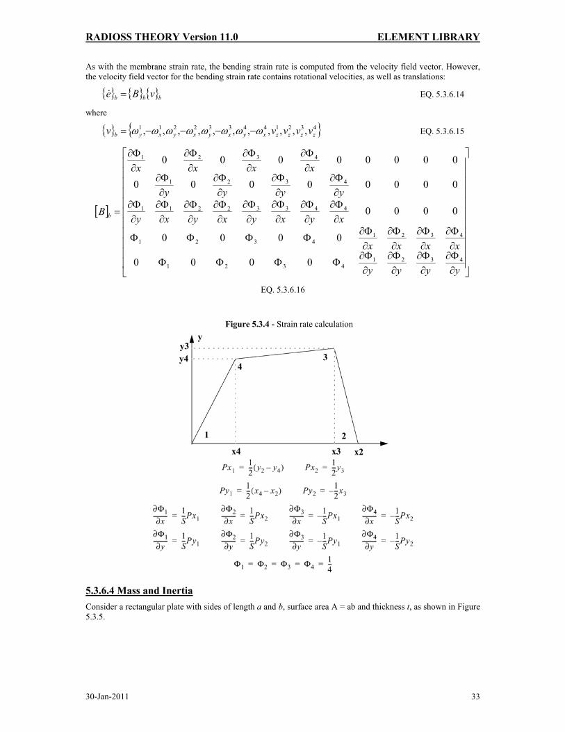
As with the membrane strain rate, the bending strain rate is computed from the velocity field vector. However, the velocity field vector for the bending strain rate contains rotational velocities, as well as translations:
{ } { } { }bbb vBe =& EQ. 5.3.6.14
where
{ } { }432144332211 ,,,,,,,,,,, zzzzxyxyxyxyb vvvvv ωωωωωωωω −−−−= EQ. 5.3.6.15
[ ]
⎥⎥⎥⎥⎥⎥⎥⎥⎥⎥⎥
⎦
⎤
⎢⎢⎢⎢⎢⎢⎢⎢⎢⎢⎢
⎣
⎡
∂Φ∂
∂Φ∂
∂Φ∂
∂Φ∂
ΦΦΦΦ
∂Φ∂
∂Φ∂
∂Φ∂
∂Φ∂
ΦΦΦΦ
∂Φ∂
∂Φ∂
∂Φ∂
∂Φ∂
∂Φ∂
∂Φ∂
∂Φ∂
∂Φ∂
∂Φ∂
∂Φ∂
∂Φ∂
∂Φ∂
∂Φ∂
∂Φ∂
∂Φ∂
∂Φ∂
=
yyyy
xxxx
xyxyxyxy
yyyy
xxxx
B b
43214321
43214321
44332211
4321
4321
0000
0000
0000
00000000
00000000
EQ. 5.3.6.16
Figure 5.3.4 - Strain rate calculation
5.3.6.4 Mass and Inertia Consider a rectangular plate with sides of length a and b, surface area A = ab and thickness t, as shown in Figure 5.3.5.

RADIOSS THEORY Version 11.0 ELEMENT LIBRARY
30-Jan-2011 34
Figure 5.3.5 - Mass Distribution
Due to the lumped mass formulation used by RADIOSS, the lumped mass at a particular node is:
Atm ρ41
= EQ. 5.3.6.17
The mass moments of inertia, with respect to local element reference frame, are calculated at node i by:
⎟⎟⎠
⎞⎜⎜⎝
⎛ +=
12
22 tbmI xx EQ. 5.3.6.18
⎟⎟⎠
⎞⎜⎜⎝
⎛ +=
12
22 tamI yy EQ. 5.3.6.19
⎟⎟⎠
⎞⎜⎜⎝
⎛ +=
12
22 bamI zz EQ. 5.3.6.20
16abmIxy −= EQ. 5.3.6.21
5.3.6.5 Inertia Stability With the exact formula for inertia (EQS 5.3.6.18 to 5.3.6.21), the solution tends to diverge for large rotation rates. Belytschko proposed a way to stabilize the solution by setting I xx = I yy , i.e. to consider the rectangle as a square with respect to the inertia calculation only. This introduces an error into the formulation. However, if the aspect ratio is small the error will be minimal. In RADIOSS a better stabilization is obtained by:
⎟⎟⎠
⎞⎜⎜⎝
⎛+=
12
2tfAmIxx EQ. 5.3.6.22
xxyyzz III == EQ. 5.3.6.23
0=xyI EQ. 5.3.6.24
where f is a regulator factor with default value f=12 for QBAT element and f=9 for other quadrilateral elements.
5.3.7 Internal forces The internal force vector is given by:
∫Ω
Ω=e
et dBf σint EQ. 5.3.7.1
x
y
z
a
b
1 2
3 4
m

RADIOSS THEORY Version 11.0 ELEMENT LIBRARY
30-Jan-2011 35
In elasticity it becomes:
∫Ω
Ω=e
etCBvdBf int EQ. 5.3.7.2
It can be written as: hgr
fff int0intint += EQ. 5.3.7.3
with the constant part 0intf being computed with one-point quadrature and the non constant part or hourglass
part hgr
f int being computed by perturbation stabilization (Ishell = 1, 2 ,3 ...) or by physical stabilization (Ishell = 22).
5.3.8 Hourglass modes Hourglass modes are element distortions that have zero strain energy. The 4 node shell element has 12 translational modes, 3 rigid body modes (1, 2, 9), 6 deformation modes (3, 4, 5, 6, 10, 11) and 3 hourglass modes (7, 8, 12).
Figure 5.3.6 - Translational Modes of Shell
Along with the translational modes, the 4 node shell has 12 rotational modes: 4 out of plane rotation modes (1, 2, 3, 4), 2 deformation modes (5, 6), 2 rigid body or deformation modes (7, 8) and 4 hourglass modes (9, 10, 11, 12).

RADIOSS THEORY Version 11.0 ELEMENT LIBRARY
30-Jan-2011 36
Figure 5.3.7 - Rotational Modes of Shell
5.3.8.1 Hourglass Viscous Forces Hourglass resistance forces are usually either viscous or stiffness related. The viscous forces relate to the rate of displacement or velocity of the elemental nodes, as if the material was a highly viscous fluid. The viscous formulation used by RADIOSS is the same as that outlined by Kosloff and Frasier [10]. Refer to section 5.1.5. An hourglass normalized vector is defined as:
( )1,1,1,1 −−=Γ EQ. 5.3.8.1
The hourglass velocity rate for the above vector is defined as:
432 iiiiIiIIi vvvvv
tq
−+−=Γ=∂∂
EQ. 5.3.8.2
The hourglass resisting forces at node I for in-plane modes are:
Ii
mhgr
iI tqAhctf Γ
∂∂
=24
1 ρ EQ. 5.3.8.3
For out of plane mode, the resisting forces are:
1041 2 fhgr
iI
hctf ρ= I
i
tq
Γ∂∂
EQ. 5.3.8.4
where
i is the direction index,
I is the node index,
t is the element thickness,
c is the sound propagation speed,
A is the element area,

RADIOSS THEORY Version 11.0 ELEMENT LIBRARY
30-Jan-2011 37
ρ is the material density,
h m is the shell membrane hourglass coefficient,
h f is the shell out of plane hourglass coefficient.
5.3.8.2 Hourglass Elastic Stiffness Forces RADIOSS can apply a stiffness force to resist hourglass modes. This acts in a similar fashion to the viscous resistance, but uses the elastic material stiffness and node displacement to determine the size of the force. The formulation is the same as that outlined by Flanagan et al. [12]. Refer to section 5.1.5.2. The hourglass resultant forces are defined as:
Ihgr
ihgr
iI ff Γ= EQ. 5.3.8.5
For membrane modes:
( ) ( ) ttqEthtfttf i
mhgr
ihgr
i Δ∂∂
+=Δ+81
EQ. 5.3.8.6
For out of plane modes:
( ) ( ) ttqEthtfttf i
fhgr
ihgr
i Δ∂∂
+=Δ+ 3
401
EQ. 5.3.8.7
where
t is the element thickness,
Δt is the time step,
E is Young's Modulus.
5.3.8.3 Hourglass Viscous Moments This formulation is analogous to the hourglass viscous force scheme. The hourglass angular velocity rate is defined for the main hourglass modes as:
4321 iiiiIiII
i
tr ωωωωω −+−=Γ=
∂∂
EQ. 5.3.8.8
The hourglass resisting moments at node I are given by:
Iirhgr
iI trcAthm Γ
∂∂
= 2
2501 ρ EQ. 5.3.8.9
where h r is the shell rotation hourglass coefficient.
5.3.9 Hourglass resistance To correct this phenomenon, it is necessary to introduce anti-hourglass forces and moments. Two possible formulations are presented hereafter.
5.3.9.1 Flanagan-Belytschko Formulation [12]
Ishell=1
In the Kosloff-Frasier formulation seen in section 5.1.5.1, the hourglass base vector αIΓ is not perfectly
orthogonal to the rigid body and deformation modes that are taken into account by the one point integration scheme. The mean stress/strain formulation of a one point integration scheme only considers a fully linear velocity field, so that the physical element modes generally contribute to the hourglass energy. To avoid this, the idea in the Flanagan-Belytschko formulation is to build an hourglass velocity field which always remains orthogonal to the physical element modes. This can be written as:

RADIOSS THEORY Version 11.0 ELEMENT LIBRARY
30-Jan-2011 38
LiniIiI
HouriI vvv −= EQ. 5.3.9.1
The linear portion of the velocity field can be expanded to give:
( )⎟⎟⎠
⎞⎜⎜⎝
⎛−⋅
∂∂
+−= jjj
iIiIiI
HouriI xx
xvvvv EQ. 5.3.9.2
Decomposition on the hourglass base vectors gives [12]:
ααα
Ijj
iIiI
HouriII
i xxvvv
tq
Γ⋅⎟⎟⎠
⎞⎜⎜⎝
⎛⋅
∂∂
−=⋅Γ=∂
∂ EQ. 5.3.9.3
where
tqi
∂∂ α
are the hourglass modal velocities,
αIΓ are the hourglass vectors, base.
Remembering that iJj
j
j
i vxx
v⋅
∂Φ∂
=∂∂
and factorizing EQ. 5.1.5.5 gives:
⎟⎟⎠
⎞⎜⎜⎝
⎛Γ
∂Φ∂
−Γ⋅=∂
∂ ααα
Jjj
JIiI
i xx
vt
q EQ. 5.3.9.4
αααγ Jjj
JII x
xΓ
∂Φ∂
−Γ= EQ. 5.3.9.5
is the hourglass shape vector used in place of αIΓ in EQ. 5.1.5.2.
Figure 5.3.8 - Flanagan Belytschko Hourglass formulation

RADIOSS THEORY Version 11.0 ELEMENT LIBRARY
30-Jan-2011 39
5.3.9.2 Elastoplastic Hourglass Forces
Ishell=3 The same formulation as elastic hourglass forces is used (section 5.3.8.2 and Flanagan et al. [12]) but the forces are bounded with a maximum force depending on the current element mean yield stress. The hourglass forces are defined as:
Ihgr
ihgr
iI ff Γ= EQ. 5.3.9.6
For in plane mode:
( ) ( ) ttqEthtfttf i
mhgr
ihgr
i Δ∂∂
+=Δ+81
EQ. 5.3.9.7
( ) ( ) ⎟⎠⎞
⎜⎝⎛ Δ+=Δ+ Athttfttf ym
hgri
hgri σ
21,min EQ. 5.3.9.8
For out of plane mode:
( ) ( ) ttqEthtfttf i
fhgr
ihgr
i Δ∂∂
+=Δ+ 3
401
EQ. 5.3.9.9
( ) ( ) ⎟⎠⎞
⎜⎝⎛ Δ+=Δ+ 2
41,min thttfttf yf
hgri
hgri σ EQ. 5.3.9.10
where:
t is the element thickness,
σy is the yield stress,
A is the element area.
5.3.9.3 Physical Hourglass Forces
Ishell=22, 24 The hourglass forces are given by:
∫Ω
Ω=e
eHHthgrvdCBBf int EQ. 5.3.9.11
For in-plane membrane rate-of-deformation, with ξη=Φ and Iγ defined in EQ 5.3.5.3:

RADIOSS THEORY Version 11.0 ELEMENT LIBRARY
30-Jan-2011 40
( )[ ]⎥⎥⎥
⎦
⎤
⎢⎢⎢
⎣
⎡=
0,,0,000,
xyy
xB
II
I
IHm
I
φγφγφγ
φγ EQ. 5.3.9.12
For bending:
( )[ ]⎥⎥⎥
⎦
⎤
⎢⎢⎢
⎣
⎡
−−=
yxy
xB
II
I
IHb
I
,,0,,0
φγφγφγ
φγ EQ. 5.3.9.13
It is shown in [16] that the non-constant part of the membrane strain rate does not vanish when a warped element
undergoes a rigid body rotation. Thus, a modified matrix [ ( )HmIB ] is chosen using I
I zz γγ = as a measure of the warping:
( )[ ]( )⎥
⎥⎥
⎦
⎤
⎢⎢⎢
⎣
⎡
+=
xyIyxIxIyI
yyIyI
xxIxIHm
I
bbzbzbz
B,,
,0,0
,,
,
,
φφφγφγφφγφφγ
γ
γ
γ
EQ. 5.3.9.14
This matrix is different from the Belytschko-Leviathan [17] correction term added at rotational positions, which couples translations to curvatures as follows:
( )[ ]⎥⎥⎥⎥⎥⎥
⎦
⎤
⎢⎢⎢⎢⎢⎢
⎣
⎡
−
−
=
yxxIyI
yyI
xxI
HmI
zz
z
z
B
,,,,
,,
,,
41
410
04100
41000
φφφγφγ
φφγ
φφγ
γγ
γ
γ
EQ. 5.3.9.15
This will lead to “membrane locking” (the membrane strain will not vanish under a constant bending loading). According to the general formulation, the coupling is presented in terms of bending and not in terms of membrane, yet the normal translation components in ( m
IB ) do not vanish for a warped element due to the
tangent vectors ( )ηξ ,it which differ from ti(0,0).
5.3.9.4 Full integrated formulation
Ishell=12 The element is based on the Q4γ24 shell element developed in [40] by Batoz and Dhatt. The element has 4 nodes with 5 local degrees-of-freedom per node. Its formulation is based on the Cartesian shell approach where the middle surface is curved. The shell surface is fully integrated with four Gauss points. Due to an in-plane reduced integration for shear, the element shear locking problems are avoided. The element without hourglass deformations is based on Mindlin-Reissner plate theory where the transversal shear deformation is taken into account in the expression of the internal energy. The reader is invited to consult the reference for more details.
5.3.9.5 Shell membrane damping The shell membrane damping, dm, is only used for law 25, 27, 19, 32 and 36. The Shell membrane damping factor is a factor on the numerical VISCOSITY and not a physical viscosity. Its effect is shown in the formula of the calculation of forces in a shell element:
dm = dm read in D00 input (Shell membrane damping factor parameter) then:
AREAcdmdm D ⋅⋅⋅⋅= 0002 ρ EQ. 5.3.9.16

RADIOSS THEORY Version 11.0 ELEMENT LIBRARY
30-Jan-2011 41
Effect in the force vector (F) calculation:
⎟⎠⎞
⎜⎝⎛ ++=
222
1111εε&
&dmFF oldnew EQ. 5.3.9.17
⎟⎠⎞
⎜⎝⎛ ++=
211
2222εε&
&dmFF oldnew EQ. 5.3.9.18
312
33ε&dmFF oldnew += EQ. 5.3.9.19
Where: 0ρ = density
AREA = area of the shell element surface
dt = time step
c = sound speed
In order to calibrate the dm value so that it represents the physical viscosity, one should obtain the same size for all shell elements (Cf. AREA factor), then scale the physical viscosity value to the element size.
5.3.10 Stress and strain calculation The stress and strain for a shell element can be written in vector notation. Each component is a stress or strain feature of the element. The generalized strain ε can be written as:
{ } { }xyyxxyyx kkkeee ,,,,,=ε EQ. 5.3.10.1
where
eij is the membrane strain,
χ ij is the bending strain or curvature.
The generalized stress Σ can be written as:
{ } { }xyyxxyyx MMMNNN ,,,,,=∑ EQ. 5.3.10.2
where: ∫−
=2/
2/
t
txx dzN σ ∫
−
−=2/
2/
t
txx zdzM σ
∫−
=2/
2/
t
tyy dzN σ ∫
−
−=2/
2/
t
tyy zdzM σ
∫−
=2/
2/
t
txyxy dzN σ ∫
−
−=2/
2/
t
txyxy zdzM σ
∫−
=2/
2/
t
tyzyz dzN σ ∫
−
=2/
2/
t
txzxz dzN σ
5.3.10.1 Isotropic Linear Elastic Stress Calculation The stress for an isotropic linear elastic shell for each time increment is computed using:
){ } ( ){ } { } ttttel Δ+∑=Δ+∑ ε&L( EQ. 5.3.10.3
RADIOSS THEORY Version 11.0 ELEMENT LIBRARY
30-Jan-2011 42
where EQ. 5.3.10.4
⎥⎦
⎤⎢⎣
⎡=
b
m
LL0
0L EQ. 5.3.10.5
⎥⎥⎥⎥⎥⎥
⎦
⎤
⎢⎢⎢⎢⎢⎢
⎣
⎡
+
−−−
−−
−
=
vEt
vEt
vvEt
vvEt
vEt
Lm
100
011
011
22
22
EQ. 5.3.10.6
( ) ( )
( ) ( )
( )⎥⎥⎥⎥⎥⎥⎥
⎦
⎤
⎢⎢⎢⎢⎢⎢⎢
⎣
⎡
+
−−−
−−
−
=
vEt
vEt
vvEt
vvEt
vEt
Lb
11200
0112112
0112112
3
2
3
2
3
2
3
2
3
EQ. 5.3.10.7
E is the Young's or Elastic Modulus,
ν is Poisson's Ratio,
t is the shell thickness.
5.3.10.2 Isotropic Linear Elastic-Plastic Stress Calculation An incremental step-by-step method is usually used to resolve the nonlinear problems due to elasto-plastic material behavior. The problem is presented by the resolution of the following equation:
( )pεε &&& −= :Cσ EQ. 5.3.10.8
( ) pyyeqy Hf εσσσσσ && ==−= ;0, 22 EQ. 5.3.10.9
0=f& EQ. 5.3.10.10
and λσ
ε &&∂∂
=f
p EQ. 5.3.10.11
f is the yield surface function for plasticity for associative hardening. The equivalent stress eqσ may be expressed in form:
{ } [ ]{ }σσσ Ateq =2 EQ. 5.3.10.12
with { }⎪⎭
⎪⎬
⎫
⎪⎩
⎪⎨
⎧
=
xy
yy
xx
σσσ
σ and [ ]⎥⎥⎥
⎦
⎤
⎢⎢⎢
⎣
⎡−
−=
3000101
21
21
A for von Mises criteria.

RADIOSS THEORY Version 11.0 ELEMENT LIBRARY
30-Jan-2011 43
The normality law (EQ. 5.3.10.11) for associated plasticity is written as:
{ } ( ) [ ]{ } [ ]{ }σσελσλ
σε AAf
y
p
p&&&& ==
∂∂
= 2 EQ. 5.3.10.13
Where pε& is the equivalent plastic deformation.
EQ. 5.3.10.8 is written in an incremental form:
{ } { } { } { } [ ]{ } { }( ) { } [ ][ ]{ } 111 ++∗
+ −=−+=+= nny
p
pnnn ACdddCd σσ
εσεεσσσσ EQ. 5.3.10.14
Where { }*σ represents stress components obtained by an elastic increment and [C] the elastic matrix in plane stress. The equations EQ. 5.3.10.8 to 14 lead to obtain the nonlinear equation:
( ) 0=pdf ε EQ. 5.3.10.15
that can be resolved by an iterative algorithm as Newton-Raphson method.
To determine the elastic-plastic state of a shell element, a number of steps have to be performed to check for yielding and defining a plasticity relationship. Stress-strain and force-displacement curves for a particular ductile material are shown in Figure 5.3.9.
Figure 5.3.9 - Material Curve

RADIOSS THEORY Version 11.0 ELEMENT LIBRARY
30-Jan-2011 44
The steps involved in the stress calculation are as follows.
1. Strain calculation at integration point z
The overall strain on an element due to both membrane and bending forces is:
xxx ze χε −= EQ. 5.3.10.16
yyy ze χε −= EQ. 5.3.10.17
xyxyxy ze χε −= EQ. 5.3.10.18
{ } { }xyyx εεεε ,,= EQ. 5.3.10.19
2. Elastic stress calculation
The stress is defined as:
{ } { }xyyx σσσσ ,,= EQ. 5.3.10.20
It is calculated using explicit time integration and the strain rate:
( ){ } ( ){ } { } ttttel Δ+=Δ+ εσσ &L EQ. 5.3.10.21
⎥⎥⎥⎥⎥⎥
⎦
⎤
⎢⎢⎢⎢⎢⎢
⎣
⎡
+
−−
−−
=
vE
vE
vvE
vvE
vE
100
011
011
L 22
22
The two shear stresses acting across the thickness of the element are calculated by:
( ) ( ) tev
Ettt yzyzelyz Δ
++=Δ+ &
1ασσ EQ. 5.3.10.22
( ) ( ) tev
Ettt xzxzelxz Δ
++=Δ+ &
1ασσ
where α is the shear factor. Default is Reissner's value of 5/6.
3. Von Mises yield criterion
The von Mises yield criterion for shell elements is defined as: 2222 3 xyyxyxvm σσσσσσ +−+= EQ. 5.3.10.23
For type 2 simple elastic-plastic material, the yield stress is calculated using:
( ) ( )tbatnp
yield εσ += EQ. 5.3.10.24
This equation will vary according to the type of material being modeled.
4. Plasticity Check
The element's state of stress must be checked to see if it has yielded. These values are compared with the von Mises and Yield stresses calculated in the previous step. If the von Mises stress is greater than the yield stress, then the material will be said to be in the plastic range of the stress-strain curve.
RADIOSS THEORY Version 11.0 ELEMENT LIBRARY
30-Jan-2011 45
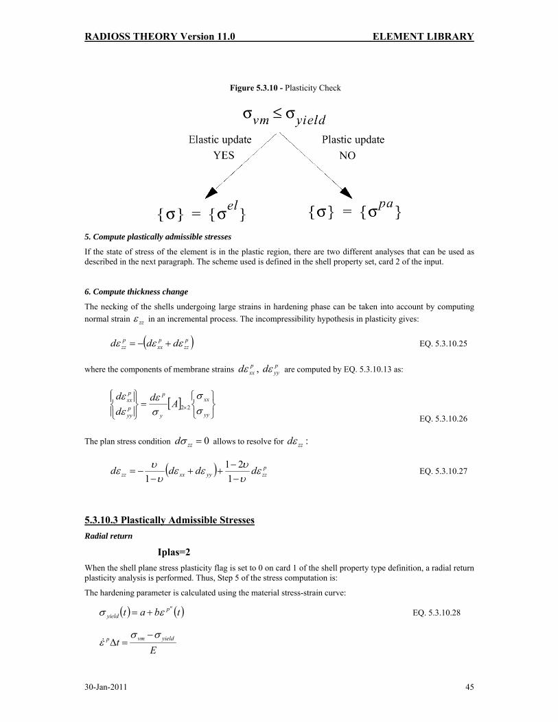
Figure 5.3.10 - Plasticity Check
5. Compute plastically admissible stresses
If the state of stress of the element is in the plastic region, there are two different analyses that can be used as described in the next paragraph. The scheme used is defined in the shell property set, card 2 of the input.
6. Compute thickness change
The necking of the shells undergoing large strains in hardening phase can be taken into account by computing normal strain zzε in an incremental process. The incompressibility hypothesis in plasticity gives:
( )pzz
pxx
pzz ddd εεε +−= EQ. 5.3.10.25
where the components of membrane strains pxxdε , p
yydε are computed by EQ. 5.3.10.13 as:
[ ]⎭⎬⎫
⎩⎨⎧
=⎪⎭
⎪⎬⎫
⎪⎩
⎪⎨⎧
×yy
xx
y
p
pyy
pxx Ad
dd
σσ
σε
εε
22
EQ. 5.3.10.26
The plan stress condition 0=zzdσ allows to resolve for zzdε :
( ) pzzyyxxzz dddd ε
υυεε
υυε
−−
++−
−=1
211
EQ. 5.3.10.27
5.3.10.3 Plastically Admissible Stresses Radial return
Iplas=2 When the shell plane stress plasticity flag is set to 0 on card 1 of the shell property type definition, a radial return plasticity analysis is performed. Thus, Step 5 of the stress computation is:
The hardening parameter is calculated using the material stress-strain curve:
( ) ( )tbatnp
yield εσ += EQ. 5.3.10.28
Et yieldvmp σσ
ε−
=Δ&

RADIOSS THEORY Version 11.0 ELEMENT LIBRARY
30-Jan-2011 46
where pε& is the plastic strain rate.
The plastic strain, or hardening parameter, is found by explicit time integration:
( ) ( ) tttt ppp Δ+=Δ+ εεε & EQ. 5.3.10.29
Finally, the plastic stress is found by the method of radial return. In case of plane stress this method is approximated because it cannot verify simultaneously the plane stress condition and the flow rule. The following return gives a plane stress state:
elij
vm
yieldpaij σ
σσ
σ = EQ. 5.3.10.30
Iterative algorithm
Iplas=1 If flag 1 is used on card 1 of the shell property type definition, an incremental method is used. Step 5 is performed using the incremental method described by Mendelson [1]. It has been extended to plane stress situations. This method is more computationally expensive, but provides high accuracy on stress distribution, especially when one is interested in residual stress or elastic return. This method is also recommended when variable thickness is being used. After some calculations, the plastic stresses are defined as:
⎟⎠⎞
⎜⎝⎛
+Δ+
−+
⎟⎠⎞
⎜⎝⎛
−Δ+
+=
vr
vr
ely
elx
ely
elxpa
x
1312
112
σσσσσ EQ. 5.3.10.31
⎟⎠⎞
⎜⎝⎛
+Δ
+
−−
⎟⎠⎞
⎜⎝⎛
−Δ
+
+=
vr
vr
ely
elx
ely
elxpa
y
1312
112
σσσσσ EQ. 5.3.10.32
vr
elxypa
xy
+Δ
+=
131
σσ EQ. 5.3.10.33
where ( )ttEr
yield
p
Δ+Δ
=Δσ
ε2
EQ. 5.3.10.34
The value of PεΔ must be computed to determine the state of plastic stress. This is done by an iterative method. To calculate the value of PεΔ , the von Mises yield criterion for the case of plane stress is introduced:
( )ttyieldxyyxyx Δ+=+−+ 2222 3 σσσσσσ EQ. 5.3.10.35
and the values of σx, σy, σxy and σyield are replaced by their expression as a function of PεΔ (EQS 5.3.8.31 to 5.3.8.34), with for example:
( ) ( )ttbattnp
yield Δ++=Δ+ εσ EQ. 5.3.10.36
and:
( ) ( ) ppp ttt εεε Δ+=Δ+ EQ. 5.3.10.37
The nonlinear equation 5.3.10.35 is solved iteratively for PεΔ by Newton's method using three iterations. This is sufficient to obtain PεΔ accurately.
RADIOSS THEORY Version 11.0 ELEMENT LIBRARY
30-Jan-2011 47
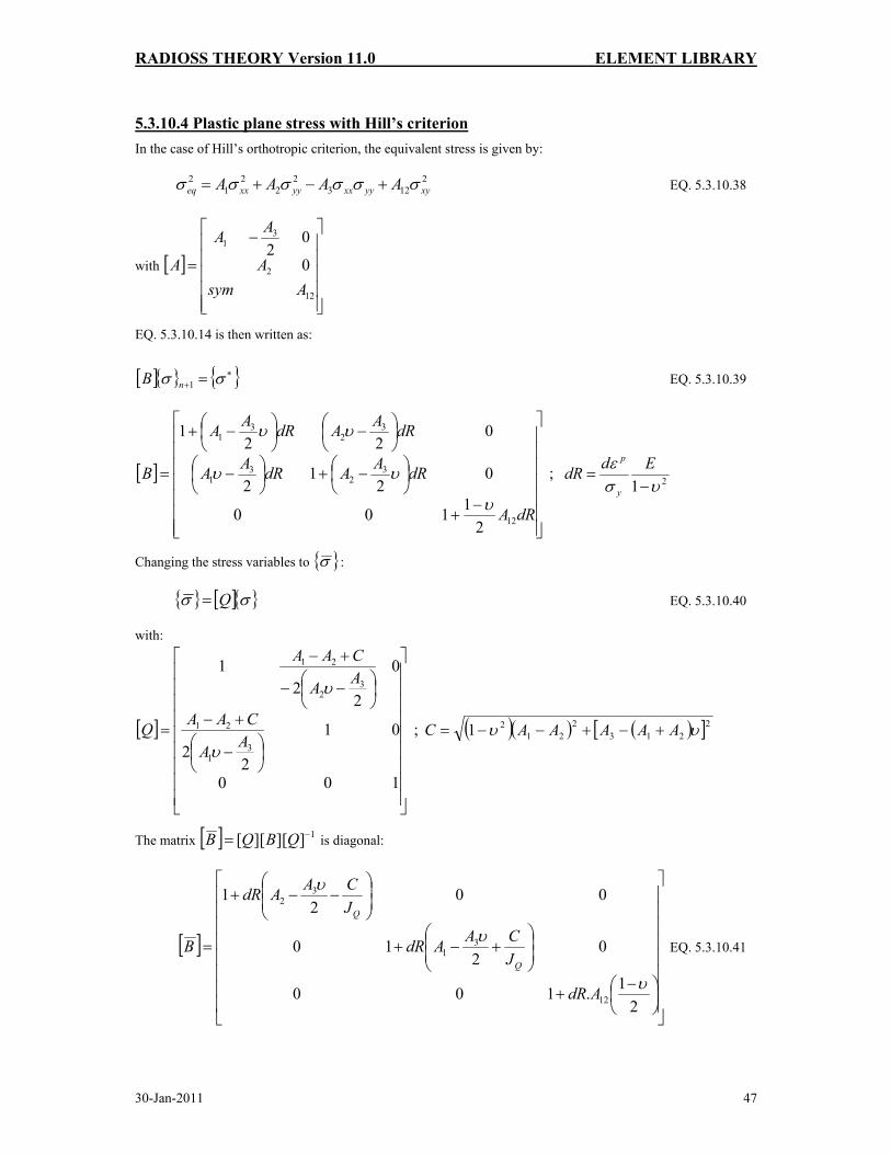
5.3.10.4 Plastic plane stress with Hill’s criterion In the case of Hill’s orthotropic criterion, the equivalent stress is given by:
2123
22
21
2xyyyxxyyxxeq AAAA σσσσσσ +−+= EQ. 5.3.10.38
with [ ]
⎥⎥⎥⎥⎥
⎦
⎤
⎢⎢⎢⎢⎢
⎣
⎡ −
=
12
2
31
0
02
AsymA
AA
A
EQ. 5.3.10.14 is then written as:
[ ]{ } { }∗
+ = σσ 1nB EQ. 5.3.10.39
[ ]
⎥⎥⎥⎥⎥⎥⎥
⎦
⎤
⎢⎢⎢⎢⎢⎢⎢
⎣
⎡
−+
⎟⎠⎞
⎜⎝⎛ −+⎟
⎠⎞
⎜⎝⎛ −
⎟⎠⎞
⎜⎝⎛ −⎟
⎠⎞
⎜⎝⎛ −+
=
dRA
dRAAdRAA
dRAAdRAA
B
12
32
31
32
31
21100
02
12
022
1
υ
υυ
υυ
; 21 υσε
−=
EddRy
p
Changing the stress variables to { }σ :
{ } [ ]{ }σσ Q= EQ. 5.3.10.40
with:
[ ]
⎥⎥⎥⎥⎥⎥⎥⎥⎥
⎦
⎤
⎢⎢⎢⎢⎢⎢⎢⎢⎢
⎣
⎡
⎟⎠⎞
⎜⎝⎛ −
+−
⎟⎠⎞
⎜⎝⎛ −−
+−
=
100
01
22
0
22
1
31
21
32
21
AA
CAA
AA
CAA
Qυ
υ
; ( )( ) ( )[ ]2213
221
21 υυ AAAAAC +−+−−=
The matrix [ ] 1]][][[ −= QBQB is diagonal:
[ ]
⎥⎥⎥⎥⎥⎥⎥⎥
⎦
⎤
⎢⎢⎢⎢⎢⎢⎢⎢
⎣
⎡
⎟⎠⎞
⎜⎝⎛ −
+
⎟⎟⎠
⎞⎜⎜⎝
⎛+−+
⎟⎟⎠
⎞⎜⎜⎝
⎛−−+
=
21.100
02
10
002
1
12
31
32
υ
υ
υ
AdR
JCAAdR
JCAAdR
BQ
Q
EQ. 5.3.10.41

RADIOSS THEORY Version 11.0 ELEMENT LIBRARY
30-Jan-2011 48
where ( )
⎟⎠⎞
⎜⎝⎛ −⎟
⎠⎞
⎜⎝⎛ −
+−+=
224
13
23
1
221
AAAA
CAAJQ
υυ is the Jacobian of [Q]. EQ. 5.3.10.40 is now written as:
[ ]{ } { }∗− = σσ 1nB EQ. 5.3.10.42
This will enable to give explicitly the expression of the yield surface EQ. 5.3.10.15:
( ) ( ) { } [ ] [ ][ ] { } ( )21121211
+∗−−∗+++ −=−= n
yttn
yneqn BABf σσσσσ
( )21
21
1222
3
1222
2
2222
1
11 +−+++= nyyyxxxyyyxx BB
ABA
BA
BA σσσσσσ EQ. 5.3.10.43
With [ ] [ ] [ ] [ ] 122222222
−××
−×× = QAQA t .
The derivative of 1+nf is carried out in order to use the Newton-Raphson method:
1
11
+
++ ′
−Δ=Δn
npn
pn f
fεε EQ. 5.3.10.44
5.3.11 Calculation of forces and moments
5.3.11.1 Integration points throughout the thickness The integration is performed using n equally spaced integration points throughout the thickness. The method used assumes a linear variation of stresses between integrations points:
∑=
=n
k
paxk
Nkx wtN
1
σ EQ. 5.3.11.1
∑=
=n
k
paxk
Mkx wtM
1
2 σ EQ. 5.3.11.2
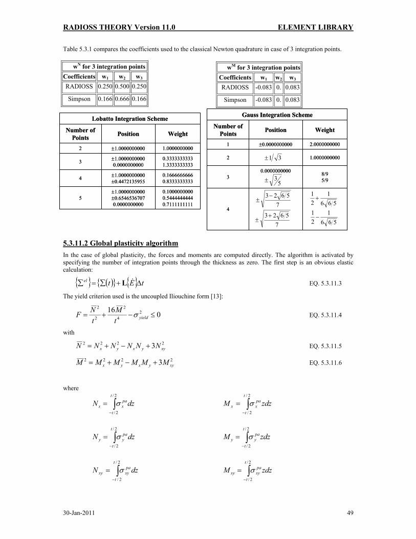
RADIOSS THEORY Version 11.0 ELEMENT LIBRARY
30-Jan-2011 49
Table 5.3.1 compares the coefficients used to the classical Newton quadrature in case of 3 integration points.
5.3.11.2 Global plasticity algorithm In the case of global plasticity, the forces and moments are computed directly. The algorithm is activated by specifying the number of integration points through the thickness as zero. The first step is an obvious elastic calculation:
{ } ( ){ } { } tEtel Δ+∑=∑ &L EQ. 5.3.11.3
The yield criterion used is the uncoupled Iliouchine form [13]:
016 24
2
2
2
≤−+= yieldtM
tNF σ EQ. 5.3.11.4
with 2222 3 xyyxyx NNNNNN +−+= EQ. 5.3.11.5
2222 3 xyyxyx MMMMMM +−+= EQ. 5.3.11.6
where
∫−
=2/
2/
t
t
paxx dzN σ ∫
−
=2/
2/
t
t
paxx zdzM σ
∫−
=2/
2/
t
t
payy dzN σ ∫
−
=2/
2/
t
t
payy zdzM σ
∫−
=2/
2/
t
t
paxyxy dzN σ ∫
−
=2/
2/
t
t
paxyxy zdzM σ
wN for 3 integration points Coefficients w1 w2 w3 RADIOSS 0.250 0.500 0.250
Simpson 0.166 0.666 0.166
wM for 3 integration points Coefficients w1 w2 w3 RADIOSS -0.083 0. 0.083
Simpson -0.083 0. 0.083
0.10000000000.54444444440.7111111111
±1.0000000000±0.65465367070.0000000000
5
0.16666666660.8333333333
±1.0000000000±0.44721359554
0.33333333331.3333333333
±1.00000000000.00000000003
1.0000000000±1.00000000002
WeightPositionNumber of Points
Lobatto Integration Scheme
0.10000000000.54444444440.7111111111
±1.0000000000±0.65465367070.0000000000
5
0.16666666660.8333333333
±1.0000000000±0.44721359554
0.33333333331.3333333333
±1.00000000000.00000000003
1.0000000000±1.00000000002
WeightPositionNumber of Points
Lobatto Integration Scheme
4
8/95/9
0.00000000003
1.00000000002
2.0000000000±0.00000000001
WeightPositionNumber of Points
Gauss Integration Scheme
4
8/95/9
0.00000000003
1.00000000002
2.0000000000±0.00000000001
WeightPositionNumber of Points
Gauss Integration Scheme
31±
53±
75623 −
±
75623+
±
5661
21
+
5661
21
−

RADIOSS THEORY Version 11.0 ELEMENT LIBRARY
30-Jan-2011 50
An extension of Iliouchine criterion for isotropic hardening is developed here. The yield surface can be expressed as:
{ }{ } [ ] { }
{ } ( ) 020 =−⎭⎬⎫
⎩⎨⎧
⎭⎬⎫
⎩⎨⎧
= βσ y
t
MN
FMN
f EQ. 5.3.11.7
with: [ ]
[ ] [ ]
[ ]⎥⎥⎥⎥⎥⎥⎥
⎦
⎤
⎢⎢⎢⎢⎢⎢⎢
⎣
⎡
⎟⎟⎠
⎞⎜⎜⎝
⎛
⎟⎟⎠
⎞⎜⎜⎝
⎛
=A
hsym
Ahhs
Ah
F22
22
6
16
32
11
γ
γ EQ. 5.3.11.8
and { } [ ]{ }{ } [ ]{ }MAN
MANs t
t
= EQ. 5.3.11.9
Where β and γ are scalar material characteristic constants, function of plastic deformation. They can be identified by the material hardening law in pure traction and pure bending:
In pure traction: ( ) ( )0
202
2
0y
py
yhNf
σεσ
ββσ =→=−= EQ. 5.3.11.10
In pure bending: ( ) ( )6/
06/ 2
2022
2
hM
hMf
yy σ
γβσγ
=→=−= EQ. 5.3.11.11
If no hardening law in pure bending is used, γ is simply computed by py
py
E
E
εσ
εσγ
+
+=
/23/
varying between 1.0
and 1.5.
The plasticity flow is written using the normality law:
{ }{ } { }
{ }
[ ] { }{ }⎭
⎬⎫
⎩⎨⎧
=
⎭⎬⎫
⎩⎨⎧
∂
∂=
⎭⎬⎫
⎩⎨⎧
Χ MN
Fd
MNfd
dd
p
p λλε
2 EQ. 5.3.11.12
The equivalent plastic deformation Pε is proportional to the plastic work. Its expression is the same as in the case of traction:
{ }{ }
{ }{ } ( )200 2 βσλ
χε
εβσ y
t
p
ppy d
MN
dd
d =⎭⎬⎫
⎩⎨⎧
⎭⎬⎫
⎩⎨⎧
= EQ.5.3.11.13
This leads to:
βλσε 02 yp dd = and p
y
dHd εσ
β 0= EQ. 5.3.11.14

RADIOSS THEORY Version 11.0 ELEMENT LIBRARY
30-Jan-2011 51
where H is the plastic module. The derivative of function f in EQ. 5.3.11.7 is discontinuous when { }tN { }{ }MA =0. This can be treated when small steps are used by putting s=0 as explained in [87].
Then the derivative of f with respect to Pdε ( Pdfε∂
∂) is carried out. The derived equation is nonlinear in
internal efforts and is resolved by Newton-Raphson:
{ }{ }
{ }{ } [ ][ ] { }
{ } 11
2+∗+ ⎭
⎬⎫
⎩⎨⎧
−⎭⎬⎫
⎩⎨⎧
=⎭⎬⎫
⎩⎨⎧
nn MN
FDdMN
MN
λ EQ. 5.3.11.15
where [D] is the elastic stiffness matrix and:
{ }{ }
{ }{ } [ ] { }
{ }⎭⎬⎫
⎩⎨⎧
−⎭⎬⎫
⎩⎨⎧
=⎭⎬⎫
⎩⎨⎧
χε
dd
DMN
MN
n*
EQ. 5.3.11.16
5.3.12 QPH, QPPS, QEPH and QBAT shell formulations QPH shell is the Belytschko Leviathan [17] shell for linear models or quasi-static analysis is identical to a QPPS shell analysis, only one difference being explained in section 5.3.12.2.
The QPPS shell is a new One-point Quadrature, General Nonlinear Quadrilateral Shell Element with Physical Stabilization. This shell is a Belytschko Leviathan [17] shell modified by Zeng and Combescure [15].
The physical stabilization is applied which enables the explicit evaluation of the stabilizing forces based on the general degenerated shell formulation and which does not require any input parameters. An optimized choice of the moduli is made in order to compute the stabilized forces for nonlinear material so that element's behavior is improved with respect to similar physical stabilization elements. The cost efficiency of the element is demonstrated by numerical examples, as compared with a fully-integrated 4-node element.
The QEPH shell is a new improved element with respect to QPH,QPPS. The improvements will be explained in section 5.3.12.2. As the QEPH is very efficient, it replaces QPH,QPPS in the applications.
The QBAT shell is a new fully-integrated 4-node element based on Q4γ 24 shell of Batoz and Dhatt [40] as discussed in section 5.3.9.4.
The general formulation of the degenerated continuum quadrilateral shell (for which all these elements used) is given in the section 5.3.12.1. The difficulties in evaluating the stabilized stiffness are also described. Section 5.3.12.2 presents the detailed formulations for the one-point quadrature shell element based on the general formulation, and compares it with that of Belytschko and Leviathan.
5.3.12.1 Formulations for a general degenerated 4-node shell The following formulations of degenerated quadrilateral shells are based on the successful full integration element MITC4 developed by Dvorkin-Bathe [32] and Q4γ 24 developed by Batoz and Dhatt [40]; they are suitable for both thin and thick shells and are applicable to linear and nonlinear problems. Their main feature is that a classical displacement method is used to interpolate the in-plane strains (membrane, bending), and a mix/collocation (or assumed strain) method is used to interpolate the out-plane strains (transverse shear). Certain conditions are also specified:
• They are based on the Reissner-Mindlin model, • In-plane strains are linear, out-plane strains(transverse shear) are constant throughout the thickness, • Thickness is constant in the element (the normal and the fiber directions are coincident), • 5 DOF in the local system (i.e. the nodal normal vectors are not constant from one element to
another).

RADIOSS THEORY Version 11.0 ELEMENT LIBRARY
30-Jan-2011 52
A - Notational conventions • A bold letter denotes a vector or a tensor. • An upper case index denotes a node number; a lower case index denotes a component of vector or
tensor. • The Einstein convention applies only for the repeated index where one is subscript and another is
superscript, e.g.: ∑= I
II
I xNxN .
• {} denotes a vector and [ ] denotes a matrix. B - Geometry and kinematics
Figure 5.3.11 - Coordinate systems
XY
Zξ
ηζ
Mid-plan a1 2
34
nr
The geometry of the 4-node degenerated shell element, as shown in the Fig 5.3.11., is defined by its mid-surface
with coordinates denoted by pX interpolated by the node coordinates IX (I=1,4):
( ) IINp X,X =ηξ EQ. 5.3.12.1
where ( )ηξ ,IN are the bilinear isoparametric shape functions, given by:
( ) ( )( ) 4/11, ηηξξηξ IIIN ++= EQ. 5.3.12.2
A generic point q within the shell is derived from point p on the mid-surface and its coordinate along the normal (fiber):
( ) nzXp,,Xq ⋅+=ζηξ with 2ζaz = EQ. 5.3.12.3
where a is the shell thickness.
The transformation between the Cartesian system and the Natural system is given by the differential relation (in matrix form):
{ } [ ] { }[( { } { }]{ } [ ]{ }ξξηξ dFdnnzFdXq =+= 0,,0 EQ. 5.3.12.4
with
[ ] { }{ } { }[ ] ( ) ( ) II,p,2
II,p,12
a210 XNXg,XNXg;nggF ηηξξ ηξηξ ===== ,,
F is the gradient tensor which is related to the Jacobian tensor [ ] [ ]tFJ = .
With 5 DOF at each node I (three translational velocities Ii
I vv → and two rotational velocities ( )Ii
I ωω → , the velocity interpolation is given by the Mindlin model:
( ) ( )( )IIIpq zβv,Nzβv,,v +=+= ηξζηξ EQ. 5.3.12.5
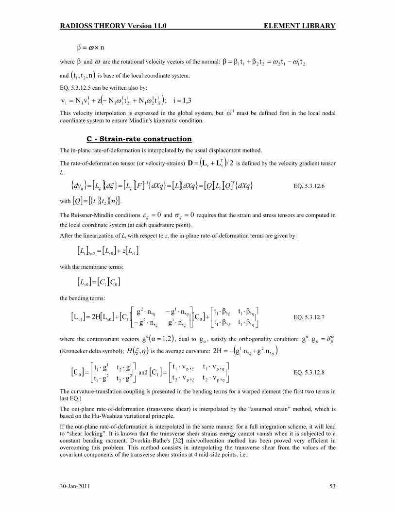
RADIOSS THEORY Version 11.0 ELEMENT LIBRARY
30-Jan-2011 53
nβ ×= ω
where β and ω are the rotational velocity vectors of the normal: 21122211 tttβtββ ωω −=+=
and ( )n,t,t 21 is base of the local coordinate system.
EQ. 5.3.12.5 can be written also by:
( ) 1,3i;tNtNzvNv I1i
I2I
I2i
I1I
IiIi =+−+= ωω
This velocity interpolation is expressed in the global system, but ω I must be defined first in the local nodal coordinate system to ensure Mindlin's kinematic condition.
C - Strain-rate construction
The in-plane rate-of-deformation is interpolated by the usual displacement method.
The rate-of-deformation tensor (or velocity-strains) ( ) 2/TtLLD += t is defined by the velocity gradient tensor
L:
{ } [ ]{ } [ ][ ] { } [ ]{ } [ ][ ][ ] { }dXqQLQdXqLdXqFLdLdv Ttq ==== −1
ζζ ξ EQ. 5.3.12.6
with [ ] { }{ }{ }[ ]nttQ 21= .
The Reissner-Mindlin conditions 0=ζε and 0=ζσ requires that the strain and stress tensors are computed in the local coordinate system (at each quadrature point).
After the linearization of Lt with respect to z, the in-plane rate-of-deformation terms are given by:
[ ] [ ] [ ]1022 sst LzLL +=×
with the membrane terms:
[ ] [ ][ ]010 CCLs =
the bending terms:
[ ] [ ] [ ] [ ] ⎥⎦
⎤⎢⎣
⎡⋅⋅⋅⋅
+⎥⎥⎦
⎤
⎢⎢⎣
⎡
⋅⋅−⋅−⋅
+=ηξ
ηξ
ξξ
ηη
β,tβ,tβ,tβ,t
Cn,gn,gn,gn,g
CL2HL11
11012
12
1s0s1 EQ. 5.3.12.7
where the contravariant vectors ( )1,2αgα = , dual to αg , satisfy the orthogonality condition: ⋅αg α
ββ δ=g
(Kronecker delta symbol); ( )ηξ ,H is the average curvature: ( )ηξ n,gn,g2H 21⋅⋅ +−=
[ ] ⎥⎦
⎤⎢⎣
⎡
⋅⋅⋅⋅
= 22
21
12
11
0 gtgtgtgt
C and [ ] ⎥⎦
⎤⎢⎣
⎡⋅⋅⋅⋅
=ηξ
ηξ
,vt,vt,vt,vt
Cp2p2
p1p11 EQ. 5.3.12.8
The curvature-translation coupling is presented in the bending terms for a warped element (the first two terms in last EQ.)
The out-plane rate-of-deformation (transverse shear) is interpolated by the “assumed strain” method, which is based on the Hu-Washizu variational principle.
If the out-plane rate-of-deformation is interpolated in the same manner for a full integration scheme, it will lead to “shear locking”. It is known that the transverse shear strains energy cannot vanish when it is subjected to a constant bending moment. Dvorkin-Bathe's [32] mix/collocation method has been proved very efficient in overcoming this problem. This method consists in interpolating the transverse shear from the values of the covariant components of the transverse shear strains at 4 mid-side points. i.e.:

RADIOSS THEORY Version 11.0 ELEMENT LIBRARY
30-Jan-2011 54
( ) ( )[ ] 2/11 21 AAξξξ γηγηγ ++−= EQ. 5.3.12.9
( ) ( )[ ] 2/11 21 BBηηη γξγξγ ++−= EQ. 5.3.12.10
Where αη
αξ γγ BA , are the values of the covariant components at 4 mid-side points which vanish under a
constant bending moment (see Figure 5.3.12).
Figure 5.3.12 - Covariant components at 4 mid-side
D - Special case for one-point quadrature and the difficulties in stabilization
The formulations described above are general for both the full integration and reduced integration schemes. For a one-point quadrature element, we have the following particularities:
The quadrature point is often chosen at ( )0,0 == ηξ . The derivatives of the shape functions are:
( ) 4/, ηξξ III hN += ( ) 4/, ξηη III hN += EQ. 5.3.12.11
Where ( )1111 −−=Ih .
This implies that all the terms computed at the quadrature point are the constant parts with respect to ( )ηξ , , and the stabilizing terms (hourglass) are the non-constant parts.
The constant parts can be derived directly from the general formulations at the quadrature point without difficulty. The difficulties in stabilization lie in correctly computing the internal force vector (or stiffness matrices):
( )∫Ω
+===Ω⋅= intintint 0 stabt ffdBf ηξσ EQ. 5.3.12.12
It would be ideal if the integration term intstabf could be evaluated explicitly. But such is not the case, and the
main obstacles are the following:
For a non-coplanar element, the normal varies at each point so that it is difficult to write the non-constant part of strains explicitly. For a physically nonlinear problem, the non-constant part of stress is not generally in an explicit form. Thus, simplification becomes necessary.
5.3.12.2 Fully-integrated shell element QBAT
QBAT is a fully-integrated shell element based on the general formulation described above. In the surface of each element, 4 Gauss points are used to evaluate the nodal forces.
1
4
3
2
B1
A2
B2
A1
A1
B1
A2
B2 ηγ
ηγ
ηγ
ξγ
ξγ
ξγ

RADIOSS THEORY Version 11.0 ELEMENT LIBRARY
30-Jan-2011 55
The main modifications with respect to Q4γ 24 shell element [40] are the following:
• Reduced integration for in-plane shear (constant) to avoid locking.
• Co-rotational coordinate system is used and the stresses are evaluated in 4 local systems at each Gauss points..
5.3.12.3 The new one-point quadrature shell element In this section, a one-point quadrature shell element formulation will be developed from the general formulation described in the previous section. It is based on the Physical Stabilization method which explicitly computes the stabilization terms in making some simplifications.
The following formulations will be written in the local coordinate system [t1 t2 n] (the circumflex in the co-rotational system notation has been omitted for convenience).
A - Kinematic approximation
The velocity interpolation using the nodal tangent vectors ( I2
I1 t,t ) complicates the strain computation, especially
for transverse shear which is used mainly as a penalty function. To be consistent with the one-point quadrature approach, the kinematic approximation is performed by:
( )[ ]Ii
Ii
IiIi zvNv 2112 ωδωδ +−+= EQ. 5.3.12.13
where Iiω (i=1,2) is the nodal rotation velocity around I
it . Iiω can be computed by a projection scheme by :
( ) ( ) IIIIIII nPnn ωωωω =⋅−= EQ. 5.3.12.14
The projection consists in eliminating the nodal drilling rotations in order to reinforce Mindlin's kinematic condition at the nodes. It has been pointed out [18] that without this projection, the element is too flexible and cannot pass the Twisted Beam test.
This projection has a drawback of changing the invariance property to rigid body motion, i.e.: a warped element being invariant to rigid body rotation will now strains under to rigid body rotation if the drill projection is applied. To overcome this problem, a full projection proposed by Belytschko-Leviathan [66] which free either drilling rotation or rigid motion should be used. This full projection is only used for QEPH element.
B - In-plane strain-rate construction
Constant part
It is useful to write the shape functions in Belytschko-Bachrach's mixed form:
( ) φγξη IyyI
xxIII bbyxN +++Δ=,, EQ. 5.3.12.15
with: ( ) ( )[ ] ( )1,1,1,1; =−−=Δ IyII
IxII
III tbytbxtt
( ) ( ) ( )( )2//;/ 3124134213423124 fjfifijAxxxxbAyyyyb yIxI −===
( ) ( )[ ] ;;4/ ξηφγ =−−= yIJ
JxIJ
JII byhbxhh
A: area of element
The derivation of the shape functions is given by:
( )yxbN III ,,, =+= αφγ ααα

RADIOSS THEORY Version 11.0 ELEMENT LIBRARY
30-Jan-2011 56
where:
ξηξηηξφ
ξηξηηξφ1
221
21
112
1,
,,,
,,11
−−
−−
+=+=
+=+=
JJ
JJ
yyy
xxx EQ. 5.3.12.16
The advantage of this shape function form is that a linear field expressed with Cartesian coordinates and a bilinear field expressed with Natural coordinates is decomposed so that the constant part is directly formulated with the Cartesian coordinates, and the non-constant part is to be approached separately.
The in-plane rate-of-deformation (decomposed on membrane and bending) is given by:
{ } { } { } [ ]{ }InI
bm vBDzDD =+= EQ. 5.3.12.17
with:
⎣ ⎦ [ ] [ ] .; >>=<<+= Iy
Ix
Iz
Iy
Ix
In
bI
mII vvvvBzBB ϖϖ
The development of the general formulations leads to the constant part, denoted by superscript 0, of the matrix
[BI]:
( )[ ]⎥⎥⎥
⎦
⎤
⎢⎢⎢
⎣
⎡
=00000
0
xIyI
yI
xImI
bbb
bB ( )[ ] ( )[ ]
⎥⎥⎥
⎦
⎤
⎢⎢⎢
⎣
⎡
−−+=
yIxIcxI
cyI
yIcyI
xIcxI
mI
b
bbbbbb
bbBHB
0000
0002 00
EQ. 5.3.12.18
with
><>=< 34122 ;;;/4 yyyy
cxI bbbbAzb γ
><>=< 12342 ;;;/4 xxxx
cyI bbbbAzb γ
The parameter II zz γγ = is a measure of the warping of the element.
The first term ( )[ ]02 mIBH is neglectable. We have verified that the order of ( )[ ]02 m
IBH is ε times the second
term of ( )[ ]0bB with ( )( ) ,2//2 3434 jiij fffyx +==ε which vanishes when the element is rectangular. Thus, this term is not used in the program.
The constant part of the in-plane rate-of-deformation formulation without the H term is consistent with the result of Belytschko's family shell element [24], [17], though this part has been obtained in a very different manner. Letellier has given the same result in his thesis [43], and studies were also made of the quadratic terms with respect to z.
Non-constant part
The main simplification for the non-constant part formulation, in order to overcome the difficulties described above, is the following:
The element is considered to be flat.
In this case, the Jacobian matrix is written as:
[ ] [ ] [ ]⎥⎦
⎤⎢⎣
⎡=
⎥⎥⎥
⎦
⎤
⎢⎢⎢
⎣
⎡==
JJaJ
JJayxyx
FJ t
2/00
2/000,,0,,
00
0 ηη
ξξ
EQ. 5.3.12.19
with the determinant J of the in-plane Jacobian:
[ ] ηξ 210det JJJJJ ++== EQ. 5.3.12.20

RADIOSS THEORY Version 11.0 ELEMENT LIBRARY
30-Jan-2011 57
and:
( )( ) ( )( )[ ] 4/16/0 AyxyxJ II
II
II
II =−= ξηηξ
( )( ) ( )( )[ ] 16/1I
II
II
II
I yxhyhxJ ξξ −=
( )( ) ( )( )[ ] 16/2I
II
II
II
I yhxyxhJ ηη −=
The inverse of the in-plane Jacobian matrix can be expressed explicitly:
[ ] ( ) ( )( ) ( ) ⎥
⎦
⎤⎢⎣
⎡
++++
=⎥⎦
⎤⎢⎣
⎡−
−=⎥
⎦
⎤⎢⎣
⎡= I
III
II
III
III
yy
xx
xhxhyhyh
Jxxyy
JJ
ηξξηηξξη
ηξηξ
ξη
ξη
41
,,,,1
,,,,
EQ. 5.3.12.21
We can now write the non-constant part, denoted by superscript H, of the matrix [BI] for in-plane rate-of-deformation:
( )[ ] ( )[ ]⎥⎥⎥
⎦
⎤
⎢⎢⎢
⎣
⎡
−−=
⎥⎥⎥
⎦
⎤
⎢⎢⎢
⎣
⎡
=
yIxI
yI
xIHb
I
xIyI
yI
xIHm
I BB,,
0,,0
;0,,0,000,
φγφγφγ
φγ
φγφγφγ
φγ EQ. 5.3.12.22
It is shown in [16] that the non-constant part of membrane rate-strain does not vanish when a warped element
undergoes a rigid body rotation. Thus, a modified matrix ( )[ ]HmIB is chosen:
( )[ ]( )⎥
⎥⎥
⎦
⎤
⎢⎢⎢
⎣
⎡
+=
xyIyxIxIyI
yyIyI
xxIxIHm
I
bbzbzbz
B,,,,
,,0,0,
φφφγφγφφγφφγ
γ
γ
γ
EQ. 5.3.12.23
This matrix is different from the Belytschko-Leviathan correction term added at rotational positions, which couples translations to curvatures as follows:
( )[ ]⎥⎥⎥⎥⎥⎥
⎦
⎤
⎢⎢⎢⎢⎢⎢
⎣
⎡
−
−
=
yxxIyI
yyI
xxI
HmI
zz
z
z
B
,41,
410,,
0,410,0
,41000,
φφφγφγ
φφγ
φφγ
γγ
γ
γ
EQ. 5.3.12.24
This will lead to 'membrane locking' (the membrane strain will not vanish under a constant bending loading). According to the general formulation, the coupling is presented in the bending terms not in the membrane terms, yet the normal translation components in (BI
m)i3 do not vanish for a warped element due to the tangent vectors ti ),( ηξ which differ from ti (0,0).
C - Out-plane strain-rate construction
The out-plane rate-of-deformation (transverse shear) is interpolated by the Dvorkin-Bathe method, whose closed form is given by Belytschko-Leviathan:
[ ]⎪⎭
⎪⎬
⎫
⎪⎩
⎪⎨
⎧
=⎭⎬⎫
⎩⎨⎧
Iy
Ix
Iz
Icyz
xzv
BDD
ϖϖ EQ. 5.3.12.25
where: [ ]( ) [ ]( ) [ ]( )ξηηζ ξηIcIcIc BBB +=,

RADIOSS THEORY Version 11.0 ELEMENT LIBRARY
30-Jan-2011 58
( ) ( ) ( )( ) ( ) ⎥
⎦
⎤⎢⎣
⎡
+−+−++−
= JkkIJJ
JkkIJJI
II
JkkIJJ
JkkIJJI
II
Ic xxhyxhxxyhyyhy
AB
ηηξηηξξηηηξηηξξηη
44
1610
( ) ( ) ( )( ) ( ) ⎥
⎦
⎤⎢⎣
⎡
++−+−+−
= JkkIJJ
JkkIJJI
II
JkkIJJ
JkkIJJI
II
Ic xxhyxhyxyhyyhy
AB
ξξηξξηηξξξηξξηηξξ
44
1610
EQ. 5.3.12.26
and ( ) ( ) ( ) ( ) ξξηη ξξηη 00; IcI
H
IcIcI
H
Ic BBBB ==
The straightforward form of [BIc] is obtained using one additional simplification:
( ) ( ) ( ) ( )0,0,0,0, ,,,, xxxx ηηξηξηξξ ==
which is true for a parallelogram element. Although this simplification is not necessary, it is justified by the fact that the transverse shear terms serve mainly as a penalty function.
D - Explicit integration of the nodal internal force vector
Elastic case
The elementary nodal force vector is computed by:
{ } [ ] [ ][ ]{ } eJnJ
t
ve II dvvBCBf ∫=int
Taking advantage of substantial orthogonality between:
• the constant in-plane fields along with the non-constant ones,
• the membrane and the bending,
• the in-plane fields and the out-plane fields,
• the decomposed non-constant out-plane fields,
we obtain:
{ } ( ){ } ( ){ }HIII fff int0intint +=
With ( ){ }0intIf the constant part being computed with one-point quadrature, and
( ){ } ( )[ ] [ ]( )[ ]{ } eJn
HJ
t
ve
HI
HI dvvBCBf ∫=int
It can be shown in the last equation that only the following scalar functions need to be integrated:
∫∫∫ === eyyeyyeyxexyexxexx dAAHdAAHdAAH ,,,,,, ,, φφφφφφ EQ. 5.3.12.27
These can be evaluated explicitly.
Defining 6 hourglass generalized rate-of-deformation q& by:
⎪⎩
⎪⎨⎧
+=+=
IzyI
IyI
my
IzxI
IxI
mx
vbzvqvbzvq
membrane 1
1
:γγ
&
& EQ. 5.3.12.28
⎪⎩
⎪⎨⎧
==
IxI
by
IyI
bx
bendingϖγϖγ
&
&: EQ. 5.3.12.29

RADIOSS THEORY Version 11.0 ELEMENT LIBRARY
30-Jan-2011 59
( ) ( )[ ] ( ) ( )[ ]( ) ( )[ ] ( ) ( )[ ]⎪⎩
⎪⎨⎧
+++−=+++−=
IyI
III
II
IxI
III
II
IzI
sy
IyI
III
II
IxI
III
II
IzI
sx
txhxtyhyvhqtxhxtyhyvhq
shearϖξηϖξηϖηξϖηξ
44
:&
& EQ. 5.3.12.30
The rate-of-deformations will be written explicitly.
The rate form of the constitutive relation is written as (stress plane for in-plane terms):
C:Dσ =&
With the assumption: the spin is constant within the element, the objectivity principle will be satisfied. The incremental computation is performed with the hourglass generalized rate-of-deformation q& , i.e.:
( ) ( ) tqqqnnn Δ+=
++211 &
Noting that if αφ, is considered as constant over a time step, it is equivalent to the incremental stress computation.
Physical nonlinear case
We will now consider an elastoplastic problem.
The elementary nodal internal force vector is now computed by:
{ } [ ] { } e
ve
tII dvBf ∫= σint
The constitutive relation is written by either a tangent form: :DCσ t=& , or a projection form: ( ),...σPσ e= ,
where ( ),...σCt is the history-dependent tangent tensor ; { } { } [ ]{ } tDC nnen Δ+= ++ 2/11 σσ is the trial stress,
and the function P consists of projecting the trial stress on the updated yield surface.
The decomposed form of the last equation is written:
{ } ( ){ } ( ){ }HIII fff int0intint +=
The constant part is computed by integration at each integration point through the thickness.
The stabilization part will be approached by relying on two hypotheses:
• Keep the same orthogonalities as in the elastic case, and
Use the unidimensional tangent modulus ( )ζtE to evaluate the non-constant rate-stress, i.e.:
{ } ( )( )[ ]{ }Ht
H DCEE /ζσ =& EQ. 5.3.12.31
where E is the Young's modulus and [ ]C is the matrix of elastic moduli.
Thus, the elastic case easily extends to the nonlinear case.
The incremental computation with the hourglass generalized rate-of-deformation q& becomes:
( ) ( ) tqqqmembrane mnmn
mn
m Δ+= ++ 2/11: &λ EQ. 5.3.12.32
( ) ( ) tqqqbending bnbn
bn
b Δ+= ++ 2/11: &λ EQ. 5.3.12.33
( ) ( ) tqqqshear snn
sn
s Δ+= ++ 2/11: & EQ. 5.3.12.34
Where ( )ζtE is obtained by the constant stress incremental computation along the thickness and ( ) EEt =ζ
in the elastic zone, and ttm EEE ;/=λ is the average value of ( )ζtE and ( ) EEtb /min ζλ = .
RADIOSS THEORY Version 11.0 ELEMENT LIBRARY
30-Jan-2011 60
For the QPH shell, λm = 1 We have maintained the key orthogonalities without any significant deterioration in performance, although the first two orthogonalities might have been slightly violated. In fact, it is simply due to these orthogonalities that a one-point quadrature element dramatically reduces the computation cost; otherwise we return to the full integration scheme.
Most of the physical stabilization elements have incorporated the following assumption:
The material response is constant within the element.
There are two alternatives to this assumption:
• to take the elastic matrix [ ]C directly:
{ } { } [ ] ( ){ } { } [ ] ( ){ } ( ){ } 000 =→+=−+=HPHHP CC εεσεεσσ &&&&&&&
which means that the plastic rate-of-deformation { }Pε& is constant within the element; or
• to take the tangent matrix [Ct] ( === ζηξ ,0 constant):
Since the components of [Ct] are generally functions of the updated stress (precisely, the stress deviator for an elastoplastic problem with an associative flow rule, which means that the stress is constant within the element.
Neither of these alternatives is theoretically perfect. Let us note that the [C] option results in a contradiction with the stress computation (which yields different results for the constant part and the non-constant part); it is more expensive and the tangent form is not generally used for constant stress computations within an explicit program. Hence, the approximation based on the above assumption is not necessary.
The choice of the moduli for the nonlinear case has not been studied for Belytschko-Leviathan's element [17], and it has been shown that this choice has little effect on the result of the “Cylindrical panel test”. In [30], the elastic tangent matrix has been used for the evaluation of the stabilizing forces.
QPH,QPPS have shown often stiffer behaviors and sometimes have certain numerical problems in crash simulations.
5.3.12.4 Advanced elasto-plastic hourglass control QEPH (Quadrilateral ElastoPlastic Physical Hourglass Control) element
With one-point integration formulation, if the non-constant part follows exactly the state of constant part for the case of elasto-plastic calculation, the plasticity will be under-estimated due to the fact that the constant equivalent stress is often the smallest one in the element and element will be stiffer. Therefore, defining a yield criterion for the non-constant part seems to be a good ideal to overcome this drawback.
From EQ. 5.3.12.16 and EQ. 5.3.12.21, we have the rate of stresses of non-constant part:
{ } [ ]{ } [ ]⎪⎭
⎪⎬
⎫
⎪⎩
⎪⎨
⎧
+⎪⎭
⎪⎬
⎫
⎪⎩
⎪⎨
⎧
=⎪⎭
⎪⎬
⎫
⎪⎩
⎪⎨
⎧
==000
,
,αξ
αξ
αη
αη
α
α
σσ
ξσσ
ηφφ
εσ y
x
y
x
yy
xxHH
i qq
CC &
&
&
&
&
&
&& EQ. 5.3.12.35
Where bm,=α corresponds to the membrane and bending terms respectively. Note that the shear terms are eliminated to avoid shear locking. The transverse shear terms can also be written as the same way:
{ }⎪⎭
⎪⎬⎫
⎪⎩
⎪⎨⎧
+⎪⎭
⎪⎬⎫
⎪⎩
⎪⎨⎧
=ξ
ξ
η
η
ττ
ξττ
ητy
x
y
xHi &
&
&
&& EQ. 5.3.12.36
We can now redefine 12 generalized hourglass stresses by integrating their rate ones, and the stress field can be expressed by:

RADIOSS THEORY Version 11.0 ELEMENT LIBRARY
30-Jan-2011 61
Membrane, bending: { } { } { } { }⎪⎭
⎪⎬
⎫
⎪⎩
⎪⎨
⎧
+⎪⎭
⎪⎬
⎫
⎪⎩
⎪⎨
⎧
+=+=00
00 αξ
αξ
αη
αη
αααα σσ
ξσσ
ησσσσ y
x
y
x
iH
iii
Shear: { } { } { } { }⎪⎭
⎪⎬⎫
⎪⎩
⎪⎨⎧
+⎪⎭
⎪⎬⎫
⎪⎩
⎪⎨⎧
+=+=ξ
ξ
η
η
ττ
ξττ
ηττττy
x
y
xi
Hiii &
&
&
&00
Even the redefinition for shear is not necessary as it is not included in the plastic yield criterion, but the same stress calculation as the constant part with the updated Lagrangian formulation is always useful when large strain is involved.
Plastic yield criterion:
The von Mises type of criterion is written by:
0),,( 22 =−= yeqf σζηξσ EQ. 5.3.12.37
for any point in the solid element, where yσ is evaluated at the quadrature point.
As only one criterion is used for the non-constant part, two choices are possible:
• taking the mean value, i.e.: ( ) ΩΩ
== ∫Ω
dff eqeqeq σσσ 1;
• taking the value by some representative points, e.g. eight Gausse points
The second choice has been used in this element.
Elasto-plastic hourglass stress calculation:
The incremental hourglass stress is computed by:
• Elastic increment
( ) ( ) [ ]{ } tC HHni
trHni Δ+=+ εσσ &1
• Check the yield criterion
• If 0≥f , the hourglass stress correction will be done by un radial return
( ) ( )( )fP trHni
Hni ,11 ++ = σσ
5.3.13 Three-node shell elements As for the four node shell element, a simple linear Mindlin Plate element formulation is used. Likewise, the use of one integration point and rigid body motion given by the time evolution of the local reference frame is applied. There is no hourglass mode in case of one integration point.
5.3.13.1 Local Reference Frame The local reference frame for the three node shell element is shown in Figure 5.3.13.

RADIOSS THEORY Version 11.0 ELEMENT LIBRARY
30-Jan-2011 62
Figure 5.3.13 - Node Shell Local Reference Frame
The vector normal to the plane of the element is defined as:
21
21
ggggn
××
= EQ. 5.3.13.1
The vector defining the local x direction is defined as edge 1-2:
1
11 g
gt = EQ. 5.3.13.2
Hence, the vector defining the local y direction is found from the cross product of the two previous vectors:
12 tnt ×= EQ. 5.3.13.3
5.3.13.2 Time Step The characteristic length for computing the critical time step is defined by:
( )31,23,12max2areaL = EQ. 5.3.13.4
Three Node Shell Shape Functions The three node shell has a linear shape functions defined as:
ycxba 1111 ++=φ EQ. 5.3.13.5
ycxba 2222 ++=φ EQ. 5.3.13.6
ycxba 3333 ++=φ EQ. 5.3.13.7
These shape functions are used to determine the velocity field in the element:
∑=
=3
1IxIIx vv φ EQ. 5.3.13.8
∑=
=3
1IyIIy vv φ EQ. 5.3.13.9
∑=
=3
1IzIIz vv φ EQ. 5.3.13.10
∑=
=3
1IxIIx ωφω EQ. 5.3.13.11

RADIOSS THEORY Version 11.0 ELEMENT LIBRARY
30-Jan-2011 63
∑=
=3
1IyIIy ωφω EQ. 5.3.13.12
∑= ∂
∂=
∂∂ 3
1IxI
Ix vxx
v φ EQ. 5.3.13.13
∑= ∂
∂=
∂∂ 3
1IxI
Ix vyy
v φ EQ. 5.3.13.14
5.3.13.4 Membrane Behavior The method used to calculate the membrane behavior and the membrane strain rates is exactly the same as that used for four node shell elements (see section 5.3.6.1).
5.3.13.5 Bending Behavior The bending behavior and calculation of the bending strain rates (or curvature rates) is the exact same method used for four node shell elements (see section 5.3.6.2).
5.3.13.6 Strain Rate Calculation The strain rate calculation for the three node shell is the same as the method used for the four node shell. However, only three nodes are accounted for. This makes the vectors and matrices smaller. The overall membrane strain rate is calculated by:
{ } { }xyyxm eeee &&&& 2,,= EQ. 5.3.13.15
{ } { }332211 ,,,,, yxyxyxm vvvvvvv = EQ. 5.3.13.16
{ } [ ] { }mmm vBe =& EQ. 5.3.13.17
where the [ ]mB matrix of shape function gradients is defined as:
[ ]
⎥⎥⎥⎥⎥⎥⎥
⎦
⎤
⎢⎢⎢⎢⎢⎢⎢
⎣
⎡
∂∂
∂∂
∂∂
∂∂
∂∂
∂∂
∂∂
∂∂
∂∂
∂∂
∂∂
=
xyxyxy
yyy
xxB m
332211
321
21
000
0000
φφφφφφ
φφφ
φφ
EQ. 5.3.13.18
where 03 =∂∂
xφ
for a shell element.
The overall bending strain or curvature rate is computed by:
{ } { }yzzxxyyxb eekkke &&&&&& 2,2,2,,= EQ. 5.3.13.19
{ } { }321332211 ,,,,,,, zzzxyxyxyb vvvv ωωωωωω −−−= & EQ. 5.3.13.20
{ } [ ] { }bmbb vBe =& EQ. 5.3.13.21

RADIOSS THEORY Version 11.0 ELEMENT LIBRARY
30-Jan-2011 64
where:
[ ]
⎥⎥⎥⎥⎥⎥⎥⎥⎥⎥⎥
⎦
⎤
⎢⎢⎢⎢⎢⎢⎢⎢⎢⎢⎢
⎣
⎡
∂∂
∂∂
∂∂
∂∂
∂∂
∂∂
∂∂
∂∂
∂∂
∂∂
∂∂
∂∂
∂∂
∂∂
∂∂
∂∂
∂∂
=
yyy
xxx
xyxyxy
yyy
xx
B
321321
321321
332211
321
21
000
000
000
000000
0000000
φφφφφφ
φφφφφφ
φφφφφφ
φφφ
φφ
EQ. 5.3.13.22
5.3.13.7 Mass and Inertia The three node shell element is considered as an element with a lumped mass. Its mass is defined as:
Atm ρ= EQ. 5.3.13.23
where:
ρ is the material density,
t is the shell thickness,
A is the reference plane surface area.
The mass moment of inertia about all axes is the same:
⎟⎟⎠
⎞⎜⎜⎝
⎛+=
1262 2tAmI xx EQ. 5.3.13.24
xxyyzz III == EQ. 5.3.13.25
0=xyI EQ. 5.3.13.26
When nodal masses need to be calculated, the distribution is determined by the shape of the element as shown in Figure 5.3.14.
Figure 5.3.14 - Mass distribution
The mass and inertia at node i are given by:
IImm ii
ii π
απα
== ; EQ. 5.3.13.27
1 2
3
1α
3α
2α

RADIOSS THEORY Version 11.0 ELEMENT LIBRARY
30-Jan-2011 65
5.3.14 Composite Shell Elements There are three different element types that can be used for modeling composites. These are:
• Type 9 Element Property - Orthotropic Shell
• Type 10 Element Property - Composite Shell
• Type 11 Element Property - Composite Shell with variable layers These elements are primarily used with the Tsai-Wu model (material law 25). They allow one global behavior or varying characteristics per layer, with varying orthotropic orientations, varying thickness and/or varying material properties, depending on which element is used. Elastic, plastic and failure modeling can be undertaken.
5.3.14.1 Transformation matrix from global to orthotropic skew If the element reference is defined by the axes X,Y and the orthotropy directions by axes 1-2, we can write:
Figure 5.3.15 - Fiber orientation
⎥⎦
⎤⎢⎣
⎡ −cssc
with c =cosθ and s = sinθ.
⎥⎦
⎤⎢⎣
⎡ −⋅⎥
⎦
⎤⎢⎣
⎡⋅⎥
⎦
⎤⎢⎣
⎡−
=⎥⎦
⎤⎢⎣
⎡cssc
cssc
YXY
XYX
εεεε
εεεε
2212
1211 EQ. 5.3.14.1
⎥⎦
⎤⎢⎣
⎡+⋅−+⋅
+⋅−+⋅⋅⎥
⎦
⎤⎢⎣
⎡−
=⎥⎦
⎤⎢⎣
⎡
YXYYXY
XYXXYX
cssccssc
cssc
εεεεεεεε
εεεε
....
2212
1211 EQ. 5.3.14.2
( )( ) ⎥
⎦
⎤⎢⎣
⎡
+−+−+⋅−+−+⋅−++⋅
=⎥⎦
⎤⎢⎣
⎡
YXYXYXYX
YXYXYXYX
ccsscssccscssccsscsc
εεεεεεεεεεεε
εεεε
..2.......2
2222
2222
2212
1211 EQ. 5.3.14.3
The strain-stress relation in orthotropy directions is written as:
{ } [ ]{ }εσ C= EQ. 5.3.14.4
[ ]⎥⎥⎥
⎦
⎤
⎢⎢⎢
⎣
⎡
= −
−
−
12
2211
12
22
21
11
1
1
1
1
0000
G
EE
EE
C ν
ν
EQ. 5.3.14.5
122211 σσσσ = ; 122211 εεεε = EQ. 5.3.14.6
The computed stresses are then projected to the element reference:

RADIOSS THEORY Version 11.0 ELEMENT LIBRARY
30-Jan-2011 66
⎥⎦
⎤⎢⎣
⎡−
⋅⎥⎦
⎤⎢⎣
⎡⋅⎥
⎦
⎤⎢⎣
⎡ −=⎥
⎦
⎤⎢⎣
⎡cssc
cssc
YYXY
XYXX
2212
1211
σσσσ
σσσσ
EQ. 5.3.14.7
5.3.14.2 Composite modeling in RADIOSS RADIOSS has been successfully used to predict the behavior of composite structures for crash and impact simulations in the automotive, rail and aeronautical industries.
The purpose of this chapter is to present the various options available in RADIOSS to model composites, as well as some modeling methods.
Modeling composites with shell elements
Composite materials with up to 100 layers may be modeled, each with different material properties, thickness, and fiber directions.
Lamina plasticity is taken into account using the Tsai-Wu criteria, which may also consider strain rate effects. Plastic work is used as a plasticity as well as rupture criterion.
Fiber brittle rupture may be taken into account in both orthotropic directions.
Delamination may be taken into account through a damage parameter in shear direction.
Modeling composites with solid elements
Solid elements may be used for composites.
Two material laws are available:
- Solid composite materials: one layer of composite is modeled with one solid element. Orthotropic characteristics and yield criteria are the same as shell elements (see above).
- A honeycomb material law is also available, featuring user defined yield curves for all components of the stress tensor and rupture strain.
Solid + shell elements
For sandwich plates, if the foam or the honeycomb is very thick, it is possible to combine composite shells for the plates and solid elements for the sandwich (see figure below).
5.3.14.3 Element orientation A global reference vector vr is used to define the fiber direction. The direction in which the material properties (or fiber direction) lay is known as the direction 1 of the local coordinate system of orthotropy. It is defined by the Φ angle, which is the angle between the local direction 1 (fiber direction) and the projection of the global vector vr as shown in Figure 5.3.16.

RADIOSS THEORY Version 11.0 ELEMENT LIBRARY
30-Jan-2011 67
Figure 5.3.16 - Fiber Direction Orientation
The shell normal defines the positive direction for φ . For elements with more than one layer, multiple φ angles can be defined.
The fiber direction orientation may be updated by two different ways:
1. constant orientation in local corotational reference frame
2. constant orientation in local isoparametric frame.
The first formulation may lead to unstable models especially in the case of very thin shells (e.g. airbag modelling). In Figure 5.3.17 the difference between the two formulations is illustrated for the case of element traction and shearing.

RADIOSS THEORY Version 11.0 ELEMENT LIBRARY
30-Jan-2011 68
Figure 5.3.17 - Fiber Direction Updating
5.3.14.4 Orthotropic shells The type 9 element property set defines orthotropic shell elements. They have the following properties:
1. Only one layer.
2. Can have up to 5 integration points1 through the thickness.
3. One orientation.
4. One material property.
5.3.14.5 Composite shell The type 10 element property set defines composite shell elements. They have the following properties:
1. Up to 100 layers can be modeled.
2. Constant layer thickness.
3. Constant reference vector.
4. Variable layer orientation.
5. Constant material properties.
Integration is performed with constant stress distribution for each layer.
Formulation 2
Formulation 1
Formulation 1
α
F α
α F
Formulation 2
Shear
Traction

RADIOSS THEORY Version 11.0 ELEMENT LIBRARY
30-Jan-2011 69
5.3.14.6 Composite shell with variable layers The type 11 element property set defines composite shell elements that allow variable layer thicknesses and materials. They have the following properties:
1. Up to 100 layers can be modeled.
2. Variable layer thicknesses.
3. Constant reference vector.
4. Variable layer orientation.
5. Variable material properties, mi2,3
Integration is performed with constant stress distribution for each layer.
1. Same integration rule as shells. 2. Material number m i must be defined as law type 25 or type 27 (not both) in material input cards. 3. Material given in the shell definition is only used for memory allocation, time step computation and interface
stiffness. It must also be defined as law 25.
5.3.14.7 Limitations When modeling a composite material, there are two strategies that may be applied. The first, and simplest, is to model the material in a laminate behavior. This involves using type 9 property shell elements. The second is to model each ply of the laminate using one integration point. This requires either a type 10 or 11 element.
Modeling using the type 9 element allows global behavior to be modeled. Input is simple, with only the reference vector as the extra information. A Tsai-Wu yield criterion and hardening law is easily obtained from the manufacturer or a test of the whole material.
Using the type 10 or 11 element, one model’s each ply in detail, with one integration point per ply and tensile failure is described in detail for each ply. However, the input requirements are complex, especially for the type 11 element.
Delamination is the separation of the various layers in a composite material. It can occur in situations of large deformation and fatigue. This phenomenon cannot be modeled in detail using shell theory. A global criterion is available in material law 25. Delamination can affect the material by reducing the bending stiffness and buckling force.
5.3.15 Three-node triangle without rotational d.o.f. (SH3N6) The need of simple and efficient element in nonlinear analysis of shells undergoing large rotations is evident in crash and sheet metal forming simulations. The constant-moment plate elements fit this need. One of the famous concepts in this field is that of Batoz et al. [40] known under DKT elements where DKT stands for Discrete Kirchhoff Triangle. The DKT12 element [40], [105] has a total of 12 d.o.f’s. The discrete Kirchhoff plate conditions are imposed at three mid-point of each side. The element makes use of rotational d.o.f. at each edge to take into account the bending effects. A simplified three-node element without rotational d.o.f. is presented in [106]. The rotational d.o.f. is computed with the help of out-of-plane translational d.o.f. in the neighbor elements. This attractive approach is used in RADIOSS in the development of element SH3N6 which based on DKT12.

RADIOSS THEORY Version 11.0 ELEMENT LIBRARY
30-Jan-2011 70
5.3.15.1 Strain computation We consider two adjacent coplanar elements with a common edge i-j as shown in Figure 5.3.19. Due to out-of-plane displacements of nodes m and k, the elements rotate around the side i-j. The angles between final and initial positions of the elements are respectively mα and kα for corresponding opposite nodes m and k.
Assuming a constant curvature for both of elements, the rotation angles mθ and kθ related to the bending of each element around the common side are obtained by:
Rhk
k 2=θ and
Rhm
m 2=θ EQ.5.3.15.1
However, for total rotation we have:
mkmk ααθθ +=+ EQ.5.3.15.2
which leads to:
( )( )mk
kmkk hh
h+
+=
ααθ and ( )
( )mk
mmkm hh
h+
+=
ααθ EQ.5.3.15.3
Figure 5.3.18 – Computation of rotational d.o.f. in SH3N6
i
j
m k hk
hm
kα
mα
kθ mθ
O
i, j

RADIOSS THEORY Version 11.0 ELEMENT LIBRARY
30-Jan-2011 71
Consider the triangle element in Figure 5.3.19. The outward normal vectors at the three sides are defined and denoted n1, n2 and n3. The normal component strain due to the bending around the element side is obtained using plate assumption:
( ) ( )
( ) ( )
( ) ( )
⎪⎪⎪⎪
⎭
⎪⎪⎪⎪
⎬
⎫
⎪⎪⎪⎪
⎩
⎪⎪⎪⎪
⎨
⎧
⎥⎥⎥
⎦
⎤
⎢⎢⎢
⎣
⎡
=⎪⎭
⎪⎬
⎫
⎪⎩
⎪⎨
⎧
++
++
++
6
5
4
3
2
1
22
22
22
3
2
1
αααααα
00000000
0000
4343
6262
5151
hhhh
hhhh
hhhh
n
n
n
γεε
EQ.5.3.15.4
The six mid-side rotations iα are related to the out-of-plane displacements of the six apex nodes as shown in Figure 5.3.20 by the following relation:
⎪⎪⎪⎪
⎭
⎪⎪⎪⎪
⎬
⎫
⎪⎪⎪⎪
⎩
⎪⎪⎪⎪
⎨
⎧
⎥⎥⎥⎥⎥⎥⎥⎥
⎦
⎤
⎢⎢⎢⎢⎢⎢⎢⎢
⎣
⎡
−−−−
−−−−
−−
−−
=
⎪⎪⎪⎪
⎭
⎪⎪⎪⎪
⎬
⎫
⎪⎪⎪⎪
⎩
⎪⎪⎪⎪
⎨
⎧
6
5
4
3
2
1
1coscos
1coscos
1coscos
1coscos
cos1cos
coscos1
6
5
4
3
2
1
wwwwww
000000000000000000
αααααα
63
1
1
2
53
2
2
3
42
1
1
2
32
1
1
2
3
1
21
3
3
2
2
3
1
hss
hrr
hqq
hhh
hhh
hhh
φφ
ψψ
γγ
ββ
ββ
ββ
EQ.5.3.15.5
where ( )321 hhh , ( )241 qhq , ( )352 rhr and ( )163 shs are respectively the heights of the triangles (1,2,3), (1,4,2), (2,5,3) and (3,6,1).
Figure 5.3.19 – Normal vectors definition
1n
2n
3n
1
2
3

RADIOSS THEORY Version 11.0 ELEMENT LIBRARY
30-Jan-2011 72
The non-null components of strain tensor in the local element reference are related to the normal components of strain by the following relation (see [40] and [106] for details):
⎪⎭
⎪⎬
⎫
⎪⎩
⎪⎨
⎧
⎥⎥⎥⎥⎥⎥⎥⎥
⎦
⎤
⎢⎢⎢⎢⎢⎢⎢⎢
⎣
⎡
⎟⎟⎠
⎞⎜⎜⎝
⎛ −⎟⎟⎠
⎞⎜⎜⎝
⎛ −⎟⎟⎠
⎞⎜⎜⎝
⎛ −⎟⎟⎠
⎞⎜⎜⎝
⎛ −⎟⎟⎠
⎞⎜⎜⎝
⎛ −⎟⎟⎠
⎞⎜⎜⎝
⎛ −
⎟⎟⎠
⎞⎜⎜⎝
⎛ −⎟⎟⎠
⎞⎜⎜⎝
⎛ −⎟⎟⎠
⎞⎜⎜⎝
⎛ −
⎟⎟⎠
⎞⎜⎜⎝
⎛ −⎟⎟⎠
⎞⎜⎜⎝
⎛ −⎟⎟⎠
⎞⎜⎜⎝
⎛ −
=⎪⎭
⎪⎬
⎫
⎪⎩
⎪⎨
⎧
3
2
1
3
21
3
12
2
13
2
31
1
32
1
23
2
3
21
2
2
13
2
1
32
2
3
12
2
2
31
2
1
23
222n
n
n
xy
yy
xx
lxx
lyy
lxx
lyy
lxx
lyy
lxx
lxx
lxx
lyy
lyy
lyy
γεε
γεε
EQ.5.3.15.6
Figure 5.3.20 – Neighbor elements for a triangle
5.3.15.2 Boundary conditions application As the side rotation of the element is computed using the out-of-plane displacement of the neighbor elements, the application of clamped or free boundary conditions needs a particular attention. It is natural to consider the boundary conditions on the edges by introducing a virtual and symmetric element outside of the edge as described in Figure 5.3.21. In the case of free rotation at the edge, the normal strain nkε is vanished. From EQ.5.3.15.4, this leads to:
mk αα −= EQ.5.3.15.7
In EQ.5.3.15.5 the fourth row of the matrix is then changed to:
[ ]00032
1
1
2 1coscoshhh −ββ EQ.5.3.15.8
1
2
3
6
5
4
1β
2β
3β
1γ
2γ2ψ
3ψ
1ϕ
3ϕ

RADIOSS THEORY Version 11.0 ELEMENT LIBRARY
30-Jan-2011 73
The clamped condition is introduced by the symmetry in out-of-plane displacement i.e. wm=wk. This implies
mk αα = . The fourth row of the matrix in EQ.5.3.15.5 is then changed to:
[ ]00032
1
1
2 1coscoshhh −−− ββ EQ.5.3.15.9
Figure 5.3.21 – Virtual element definition for boundary conditions application
1
2
3
6
5 4
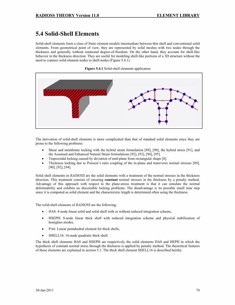
RADIOSS THEORY Version 11.0 ELEMENT LIBRARY
30-Jan-2011 74
5.4 Solid-Shell Elements Solid-shell elements form a class of finite element models intermediate between thin shell and conventional solid elements. From geometrical point of view, they are represented by solid meshes with two nodes through the thickness and generally without rotational degree-of-freedom. On the other hand, they account for shell-like behavior in the thickness direction. They are useful for modeling shell-like portions of a 3D structure without the need to connect solid element nodes to shell nodes (Figure 5.4.1).
Figure 5.4.1 Solid-shell elements application
The derivation of solid-shell elements is more complicated than that of standard solid elements since they are prone to the following problems:
• Shear and membrane locking with the hybrid strain formulation [89], [90], the hybrid stress [91], and the Assumed and Enhanced Natural Strain formulations [92], [93], [94], [95].
• Trapezoidal locking caused by deviation of mid-plane from rectangular shape [8]. • Thickness locking due to Poisson’s ratio coupling of the in-plane and transverse normal stresses [89],
[90], [92], [94]. Solid shell elements in RADIOSS are the solid elements with a treatment of the normal stresses in the thickness direction. This treatment consists of ensuring constant normal stresses in the thickness by a penalty method. Advantage of this approach with respect to the plane-stress treatment is that it can simulate the normal deformability and exhibits no discernible locking problems. The disadvantage is its possible small time step since it is computed as solid element and the characteristic length is determined often using the thickness.
The solid-shell elements of RADIOSS are the following:
• HA8: 8-node linear solid and solid-shell with or without reduced integration scheme,
• HSEPH: 8-node linear thick shell with reduced integration scheme and physical stabilization of hourglass modes,
• PA6: Linear pentahedral element for thick shells,
• SHELL16: 16-node quadratic thick shell.
The thick shell elements HA8 and HSEPH are respectively the solid elements HA8 and HEPH in which the hypothesis of constant normal stress through the thickness is applied by penalty method. The theoretical features of these elements are explained in section 5.1. The thick shell element SHELL16 is described hereby.
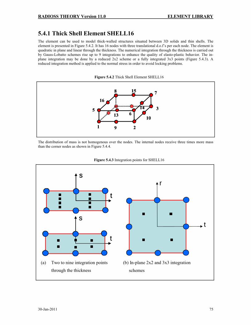
RADIOSS THEORY Version 11.0 ELEMENT LIBRARY
30-Jan-2011 75
5.4.1 Thick Shell Element SHELL16 The element can be used to model thick-walled structures situated between 3D solids and thin shells. The element is presented in Figure 5.4.2. It has 16 nodes with three translational d.o.f’s per each node. The element is quadratic in plane and linear through the thickness. The numerical integration through the thickness is carried out by Gauss-Lobatto schemes rise up to 9 integrations to enhance the quality of elasto-plastic behavior. The in-plane integration may be done by a reduced 2x2 scheme or a fully integrated 3x3 points (Figure 5.4.3). A reduced integration method is applied to the normal stress in order to avoid locking problems.
Figure 5.4.2 Thick Shell Element SHELL16
1 2
356
78
9
101314
15
16
1 2
356
78
9
101314
15
16
The distribution of mass is not homogenous over the nodes. The internal nodes receive three times more mass than the corner nodes as shown in Figure 5.4.4.
Figure 5.4.3 Integration points for SHELL16
t
r
t
s
t
s
t
s
t
s
t
s
(a) Two to nine integration points
through the thickness
(b) In-plane 2x2 and 3x3 integration
schemes

RADIOSS THEORY Version 11.0 ELEMENT LIBRARY
30-Jan-2011 76
Figure 5.4.4 Mass distribution for SHELL16 element
1/32 Mo
3/32 Mo
1/32 Mo
3/32 Mo
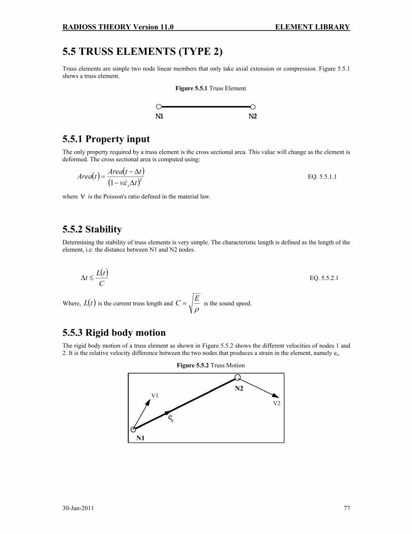
RADIOSS THEORY Version 11.0 ELEMENT LIBRARY
30-Jan-2011 77
5.5 TRUSS ELEMENTS (TYPE 2) Truss elements are simple two node linear members that only take axial extension or compression. Figure 5.5.1 shows a truss element.
Figure 5.5.1 Truss Element
5.5.1 Property input The only property required by a truss element is the cross sectional area. This value will change as the element is deformed. The cross sectional area is computed using:
( ) ( )( )21 tv
ttAreatAreaxΔ−
Δ−=
ε& EQ. 5.5.1.1
where ν is the Poisson's ratio defined in the material law.
5.5.2 Stability Determining the stability of truss elements is very simple. The characteristic length is defined as the length of the element, i.e. the distance between N1 and N2 nodes.
( )C
tLt ≤Δ EQ. 5.5.2.1
Where, ( )tL is the current truss length and ρEC = is the sound speed.
5.5.3 Rigid body motion The rigid body motion of a truss element as shown in Figure 5.5.2 shows the different velocities of nodes 1 and 2. It is the relative velocity difference between the two nodes that produces a strain in the element, namely ex.
Figure 5.5.2 Truss Motion

RADIOSS THEORY Version 11.0 ELEMENT LIBRARY
30-Jan-2011 78
F
0
logll
gap
5.5.4 Strain The strain rate, as shown in Figure 5.5.2, is defined as:
( )xeV
xv xx
x ∂⋅∂
=∂∂
=rr
&ε EQ. 5.5.4.1
5.5.5 Material type A truss element may only be assigned two types of material properties. These are types 1 and 2, elastic and elasto-plastic properties respectively.
5.5.6 Force calculation The calculation of forces in a truss element is performed by explicit time integration:
( ) ( ) tFtFttF Δ+=Δ+ & EQ. 5.5.6.1
A generalized force-strain graph can be seen in Figure 5.5.3. The force rate under elastic deformation is given by:
xx EAF ε&& = EQ. 5.5.6.2
where:
E is the Elastic Modulus,
A is the cross sectional area.
In the plastic region, the force rate is given by:
xtx AEF ε&& = EQ. 5.5.6.3
where Et is the gradient of the material curve at the deformation point.
Figure 5.5.3 Force-Strain Relationship
(a) without gap (b) with gap
In a general case, it is possible to introduce a gap distance in the truss definition. If gap is not null, the truss is activated when the length of the element is equal to the initial length minus the gap value. This results a force-strain curve shown in Figure 5.5.3(b).

RADIOSS THEORY Version 11.0 ELEMENT LIBRARY
30-Jan-2011 79
5.6 BEAM ELEMENTS (TYPE 3) RADIOSS uses a shear beam theory or Timoshenko formulation for its beam elements.
This formulation assumes that the internal virtual work rate is associated with the axial, torsional and shear strains. The other assumptions are:
• No cross section deformation in its plane.
• No cross section warping out of its plane.
With these assumptions, transverse shear is taken into account.
This formulation can degenerate into a standard Euler-Bernoulli formulation (the cross section remains normal to the beam axis). This choice is under user control.
5.6.1 Local coordinate system The properties describing a beam element are all defined in a local coordinate system.
This coordinate system can be seen in Figure 5.6.1. Nodes 1 and 2 of the element are used to define the local X axis, with the origin at node 1. The local Y axis is defined using node 3, which lies in the local XY plane, along with nodes 1 and 2. The Z axis is determined from the vector cross product of the positive X and Y axes.
The local Y direction is first defined at time t=0 and its position is corrected at each cycle, taking into account the mean rotation of the X axis. The Z axis is always orthogonal to the X and Y axes.
Deformations are computed with respect to the local coordinate system displaced and rotated to take into account rigid body motion. Translational velocities V and angular velocities Ω with respect to the global reference frame are expressed in the local frame.
Figure 5.6.1 Beam Element Local Axis
5.6.2 Beam element geometry The beam geometry is user defined by:
A: cross section area,
Ix: moment of inertia of cross section about local x axis,
Iy: moment of inertia of cross section about local y axis,
Iz: moment of inertia of cross section about local z axis.

RADIOSS THEORY Version 11.0 ELEMENT LIBRARY
30-Jan-2011 80
The moments of inertia about the y and z axes are concerned with bending. They can be calculated using the relationships:
∫∫=A
y dydzzI 2 EQ. 5.6.2.1
∫∫=A
z dydzyI 2 EQ. 5.6.2.2
The moment of inertia about the x axis concerns torsion. This is simply the summation of the previous two moments of Ontario:
zyx III += EQ. 5.6.2.3
5.6.3 Minimum time step The minimum time step for a beam element is determined using the following relation:
caLt =Δ EQ. 5.6.3.1
where:
c is the speed of sound : ρ/E ,
( ) 21 3/12/1,4min5.0 FbFba += ,
( )( )
),max(
)1(***6/5
*121*12,1max*
221,min
2212
12
21
fm
s
ss
ddd
IshearbGE
bdd
ddFF
ddF
=
⎟⎟⎠
⎞⎜⎜⎝
⎛−+=
−⎟⎠⎞⎜
⎝⎛ +=
−+=
( )zy IIALb
,max
2
=
5.6.4 Beam element behavior RADIOSS beam elements behaves in four individual ways:
• Membrane or axial deformation.
• Torsion.
• Bending about the z axis.
• Bending about the y axis.
5.6.4.1 Membrane behavior Membrane or axial behavior is the extension or compression of the beam element. The forces acting on an element are shown in Figure 5.6.2.
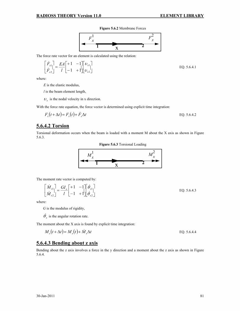
RADIOSS THEORY Version 11.0 ELEMENT LIBRARY
30-Jan-2011 81
Figure 5.6.2 Membrane Forces
The force rate vector for an element is calculated using the relation:
⎥⎦
⎤⎢⎣
⎡⎥⎦
⎤⎢⎣
⎡+−−+
=⎥⎦
⎤⎢⎣
⎡
2
1
2
1
1111
x
x
x
x
lEA
FF
υυ
&
& EQ. 5.6.4.1
where:
E is the elastic modulus,
l is the beam element length,
xυ is the nodal velocity in x direction.
With the force rate equation, the force vector is determined using explicit time integration:
( ) ( ) tFtFttF xxx Δ+=Δ+ & EQ. 5.6.4.2
5.6.4.2 Torsion Torsional deformation occurs when the beam is loaded with a moment M about the X axis as shown in Figure 5.6.3.
Figure 5.6.3 Torsional Loading
The moment rate vector is computed by:
⎥⎦
⎤⎢⎣
⎡⎥⎦
⎤⎢⎣
⎡+−−+
=⎥⎦
⎤⎢⎣
⎡
2
1
2
1
1111
x
xx
x
x
lGI
MM
θθ&
&
&
& EQ. 5.6.4.3
where:
G is the modulus of rigidity,
xθ& is the angular rotation rate.
The moment about the X axis is found by explicit time integration:
( ) ( ) tMtMttM xxx Δ+=Δ+ & EQ. 5.6.4.4
5.6.4.3 Bending about z axis Bending about the z axis involves a force in the y direction and a moment about the z axis as shown in Figure 5.6.4.
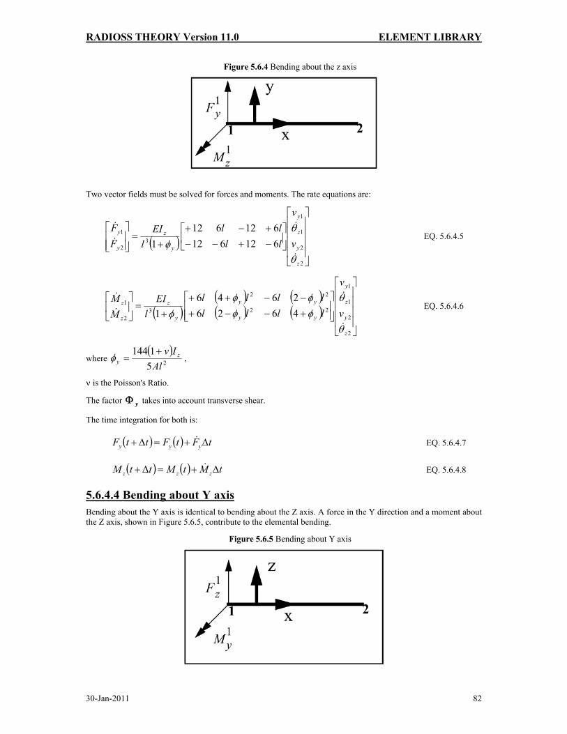
RADIOSS THEORY Version 11.0 ELEMENT LIBRARY
30-Jan-2011 82
Figure 5.6.4 Bending about the z axis
Two vector fields must be solved for forces and moments. The rate equations are:
( )⎥⎥⎥⎥
⎦
⎤
⎢⎢⎢⎢
⎣
⎡
⎥⎦
⎤⎢⎣
⎡−+−−+−+
+=
⎥⎥⎦
⎤
⎢⎢⎣
⎡
2
2
1
1
32
1
612612612612
1
z
y
z
y
y
z
y
y
v
v
llll
lEI
FF
θ
θφ
&
&
&
& EQ. 5.6.4.5
( )( ) ( )( ) ( )
⎥⎥⎥⎥
⎦
⎤
⎢⎢⎢⎢
⎣
⎡
⎥⎥⎦
⎤
⎢⎢⎣
⎡
+−−+−−++
+=⎥
⎦
⎤⎢⎣
⎡
2
2
1
1
22
22
32
1
46262646
1
z
y
z
y
yy
yy
y
z
z
z
v
v
llllllll
lEI
MM
θ
θφφφφ
φ&
&
&
& EQ. 5.6.4.6
where ( )
251144Al
Iv zy
+=φ ,
ν is the Poisson's Ratio.
The factor yΦ takes into account transverse shear.
The time integration for both is:
( ) ( ) tFtFttF yyy Δ+=Δ+ & EQ. 5.6.4.7
( ) ( ) tMtMttM zzz Δ+=Δ+ & EQ. 5.6.4.8
5.6.4.4 Bending about Y axis Bending about the Y axis is identical to bending about the Z axis. A force in the Y direction and a moment about the Z axis, shown in Figure 5.6.5, contribute to the elemental bending.
Figure 5.6.5 Bending about Y axis

RADIOSS THEORY Version 11.0 ELEMENT LIBRARY
30-Jan-2011 83
The rate equations are:
⎥⎥⎥⎥⎥
⎦
⎤
⎢⎢⎢⎢⎢
⎣
⎡
⎥⎦
⎤⎢⎣
⎡−+
+−
−−+
Φ+=⎥
⎦
⎤⎢⎣
⎡
2
2
1
1
32
1
66
1212
66
1212
)1(
y
z
y
z
z
y
z
z
ll
ll
lEl
FF
θνθν
&
&
&
& EQ. 5.6.4.9
( )( )
( )( )
⎥⎥⎥⎥⎥
⎦
⎤
⎢⎢⎢⎢⎢
⎣
⎡
⎥⎦
⎤⎢⎣
⎡
Φ+Φ−
−−
Φ−Φ+
++
Φ+=
⎥⎥⎦
⎤
⎢⎢⎣
⎡
2
2
1
1
2
2
2
2
32
1
42
66
24
66
)1(
y
z
y
z
z
z
z
z
z
y
y
y
ll
ll
ll
ll
lEl
MM
θνθν
&
&
&
& EQ. 5.6.4.10
where:
( )25
1144Al
I yz
ν+=Φ .
Like bending about the Z axis, the factor zΦ introduces transverse shear.
With the time integration, the expression is:
( ) ( ) tFtFttF zzz Δ+=Δ+ & EQ. 5.6.4.11
( ) ( ) tMtMttM yyy Δ+=Δ+ & EQ. 5.6.4.12
5.6.5 Material properties A beam element may have two different types of material property:
• Elastic
• Elasto-plastic
5.6.5.1 Elastic Behavior The elastic beam is defined using material law 1 which is a simple linear material law.
The cross-section of a beam is defined by its area A and three moments of inertia Ix , Iy and Iz .
An elastic beam can be defined with these four parameters. For accuracy and stability, the following limitations should be respected:
AL > EQ. 5.6.5.1
22 10001.0 AIA y << EQ. 5.6.5.2
22 10001.0 AIA z << EQ. 5.6.5.3
( ) ( )zyxzy IIIII +<<+ 101.0 EQ. 5.6.5.4

RADIOSS THEORY Version 11.0 ELEMENT LIBRARY
30-Jan-2011 84
5.6.5.2 Elasto-plastic Behavior A global plasticity model is used.
The main assumption is that the beam cross section is full and rectangular. Optimal relations between sections and section inertia are:
412 AII zy = EQ. 5.6.5.5
zyx III += EQ. 5.6.5.6
However, this model also gives good results for the circular or ellipsoidal cross-section. For tubular or H cross-sections, plasticity will be approximated.
Recommendations:
AL > EQ. 5.6.5.7
44 10121.0 AIIA zy << EQ. 5.6.5.8
100/01.0 << zy II EQ. 5.6.5.9
( ) ( )zyxzy IIIII +<<+ 25.0 EQ. 5.6.5.10
5.6.5.3 Global Beam Plasticity The elasto-plastic beam element is defined using material law 2:
( ) ⎟⎟⎠
⎞⎜⎜⎝
⎛++=
0
ln1εεεσ&
&CBA n
py EQ. 5.6.5.11
The increment of plastic strain is:
y
plasticp
Wσ
εΔ
=Δ EQ. 5.6.5.12
The equivalent strain rate is derived from the total energy rate:
tW
eq
total
ΔΔ
=σ
ε& EQ. 5.6.5.13
Yield stress:
⎟⎟⎠
⎞⎜⎜⎝
⎛+++=
zz
z
yy
y
xx
xxeq I
MIM
IM
AAF 222
2
2 3σ EQ. 5.6.5.14
If yeq σσ > , one performs a radial return on the yield surface:
eq
yx
pax FF
σσ
= EQ. 5.6.5.15
and for i= x, y, z:
eq
yi
pai MM
σσ
= EQ. 5.6.5.16

RADIOSS THEORY Version 11.0 ELEMENT LIBRARY
30-Jan-2011 85
5.6.6 Inertia Computation The computational method of inertia for some kinds of elements as beam is particular as the inertia has to be transferred to the extremities of the beam. The nodal inertias are computed in function of the material density ρ , the cross-section area S, the element length L and the moments of inertia zzyyxx III ,, :
( ) ⎟⎟⎠
⎞⎜⎜⎝
⎛•⎟
⎠⎞
⎜⎝⎛•⎟
⎠⎞
⎜⎝⎛+⎟⎟
⎠
⎞⎜⎜⎝
⎛⎟⎠⎞
⎜⎝⎛
xxzzyy ILIIMAXLLSLMAX2
;;2122
2 ρρρ EQ. 5.6.6.1

RADIOSS THEORY Version 11.0 ELEMENT LIBRARY
30-Jan-2011 86
5.7 ONE DEGREE OF FREEDOM SPRING ELEMENTS (TYPE 4) One degree of freedom (DOF) spring elements are defined as a type 4 property set. Three variations of the element are possible:
• Spring only
• Dashpot (damper) only
• Spring and dashpot in parallel These three configurations are shown in Figures 5.7.1 to 5.7.3.
Figure 5.7.1 Spring Only
Figure 5.7.2 Dashpot Only
Figure 5.7.3 Spring and Dashpot in Parallel
No material data card is required for spring elements. However, the stiffness k and equivalent viscous damping coefficient c are required. The mass m is required if there is any spring translation.
There are three other options defining the type of spring stiffness with the hardening flag:
• Linear Stiffness
• Nonlinear Stiffness
• Nonlinear Elasto-Plastic Stiffness

RADIOSS THEORY Version 11.0 ELEMENT LIBRARY
30-Jan-2011 87
Likewise, the damping can be either:
• Linear
• Nonlinear A spring may also have zero length. However, a one DOF spring must have 2 nodes.
The forces applied on the nodes of a one DOF spring are always colinear with direction through both nodes; refer to figure 5.7.4.
Figure 5.7.4 Colinear Forces
5.7.1 Time step The time of a spring element depends on the values of stiffness, damping and mass.
For a spring only element:
kmt =Δ EQ. 5.7.1.1
For a dashpot only element:
cmt2
=Δ EQ. 5.7.1.2
For a parallel spring and dashpot element:
( )k
ccmkt −+=Δ
2
EQ. 5.7.1.3
The critical time step ensures that the stability of the explicit time integration is maintained, but it does not ensure high accuracy of spring vibration behavior. Only two time steps are required during one vibration period of a free spring to keep stability. However, if true sinusoidal reproduction is desired, the time step should be reduced by a factor of at least 5.
If the spring is used to connect the two parts, the spring vibration period increases and the default spring time step ensures stability and accuracy.
5.7.2 Linear spring Function number defining f(δ)
N1=0

RADIOSS THEORY Version 11.0 ELEMENT LIBRARY
30-Jan-2011 88
The general linear spring is defined by constant mass, stiffness and damping. These are all required in the property type definition. The relationship between force and spring displacement is given by:
( )dtdlcllkF +−= 0 EQ. 5.7.2.1
Figure 5.7.5 Linear Force-Displacement Curve
The stability condition is given by equation 5.7.1.3.:
( )k
ckmct −+=Δ
2
EQ. 5.7.2.2
5.7.3 Nonlinear elastic spring Hardening flag
H=0 The hardening flag must be set to 0 for a nonlinear elastic spring. The only difference between linear and non linear elastic spring elements is the stiffness definition. The mass and damping are defined as constant. However, a function must be defined that relates the force, F, to the displacement of the spring, (l-l0). It is defined as:
( )dtdlcllfF +−= 0 EQ. 5.7.3.1

RADIOSS THEORY Version 11.0 ELEMENT LIBRARY
30-Jan-2011 89
Figure 5.7.6 Nonlinear Elastic Force-Displacement Curve
The stability criterion is the same as for the linear spring, but rather than being constant, the stiffness is displacement dependent:
( )k
cmkct′
−′+=Δ
2
EQ. 5.7.3.2
where:
( ) ( )⎥⎦
⎤⎢⎣
⎡−
−∂∂
=′ 00
max llfll
k EQ. 5.7.3.3
5.7.4 Nonlinear elasto-plastic spring - Isotropic hardening H=1
The hardening flag must be set to 1 in this case and f(l-l o ) is defined by a function. Hardening is isotropic if compression behavior is identical to tensile behavior:
( )dtdlCllfF +−= 0 EQ. 5.7.4.1
Figure 5.7.7 Isotropic Hardening Force-Displacement Curve

RADIOSS THEORY Version 11.0 ELEMENT LIBRARY
30-Jan-2011 90
5.7.5 Nonlinear elasto-plastic spring - Decoupled hardening H=2
The hardening flag is set to 2 in this case and f(l-l o ) is defined by a function. The hardening is decoupled for compression and tensile behavior:
( )dtdlCllfF +−= 0 EQ. 5.7.5.1
Figure 5.7.8 Decoupled Hardening Force-Displacement Curve
5.7.6 Nonlinear elastic-plastic spring - Kinematic hardening H=4
The hardening flag is set to 4 in this case and f1(l-l o ) and f2(l-l o ) (respectively maximum and minimum yield force) are defined by a function. The hardening is kinematic if maximum and minimum yield curves are identical:
( )dtdlCllfF +−= 0 EQ. 5.7.6.1
Figure 5.7.9 Kinematic Hardening Force-Displacement Curve

RADIOSS THEORY Version 11.0 ELEMENT LIBRARY
30-Jan-2011 91
5.7.7 Nonlinear elasto-plastic spring - Non linear unloading H=5
The hardening flag is set to 5 in this case and f(δ) and f2(δmax) (respectively maximum yield force and residual deformation) are defined by a function. Uncoupled hardening in compression and tensile behavior with nonlinear unloading:
( )dtdlCllfF +−= 0 EQ. 5.7.7.1
With δ= l-l o .
Figure 5.7.10 Nonlinear unloading Force-Displacement Curve
5.7.8 Nonlinear dashpot The input properties for a nonlinear dashpot are very close to that of a spring. The required values are:
• Mass, M.
• A function defining the change in force with respect to the spring displacement. This must be equal to unity:
( ) 10 =− llf
• A function defining the change in force with spring displacement rate, ( )dtdlg /
• The hardening flag in the input must be set to zero. The relationship between force and spring displacement and displacement rate is:
( ) ⎟⎠⎞
⎜⎝⎛=⎟
⎠⎞
⎜⎝⎛−=
dtdlg
dtdlgllfF 0 EQ. 5.7.8.1
A nonlinear dashpot property is shown in Figure 5.7.11.

RADIOSS THEORY Version 11.0 ELEMENT LIBRARY
30-Jan-2011 92
Figure 5.7.11 Nonlinear Dashpot Force Curve
The stability condition for a nonlinear dashpot is given by:
CMt
′=Δ EQ. 5.7.8.2
where:
( ) ( )⎥⎦
⎤⎢⎣
⎡∂
∂=′ dtdlg
dtdlC /
/max EQ. 5.7.8.3
5.7.9 Nonlinear viscoelastic spring The input properties for a nonlinear viscoelastic spring are:
• Mass, M
• Equivalent viscous damping coefficient C
• A function defining the change in force with spring displacement ( )0llf −
• A function defining the change in force with spring displacement rate ( )dtdlg /
The hardening flag in the input must be set to equal zero. The force relationship is given by:
( ) ⎟⎠⎞
⎜⎝⎛−=
dtdlgllfF 0 EQ. 5.7.9.1
Graphs of this relationship for various values of ( )dtdlg / are shown in Figure 5.7.12.

RADIOSS THEORY Version 11.0 ELEMENT LIBRARY
30-Jan-2011 93
Figure 5.7.12 Visco-Elastic Spring Force-Displacement Curves
The stability condition is given by:
( )k
CMkCt′
′−′+′=Δ
2
EQ. 5.7.9.2
where:
( ) ( )⎥⎦
⎤⎢⎣
⎡−
−∂∂
=′ 00
max llfll
K EQ. 5.7.9.3
( ) ( )⎥⎦
⎤⎢⎣
⎡∂
∂=′ dtdlg
dtdlC /
/max EQ. 5.7.9.4

RADIOSS THEORY Version 11.0 ELEMENT LIBRARY
30-Jan-2011 94
5.8 GENERAL SPRING ELEMENTS (TYPE 8) General spring elements are defined as type 8 element property. They are mathematical elements, which have 6 DOF, three translational displacements and three rotational degrees of freedom. Each DOF is completely independent from the others. Spring displacements refer to either spring extension or compression. The stiffness is associated to each DOF. Directions can either be global or local. Local directions are defined with a fixed or moving skew frame. Global force equilibrium is respected, but without global moment equilibrium. Therefore, this type of spring is connected to the laboratory that applies the missing moments, unless the two defining nodes are not coincident.
5.8.1 Time step The time step calculation for general spring elements is the same as the calculation of the equivalent type 4 spring (see section 5.7.1).
5.8.2 Linear spring See section 5.7.2; the explanation is the same as for spring type 4.
5.8.3 Nonlinear elastic spring See section 5.7.3; the explanation is the same as for spring type 4.
5.8.4 Nonlinear elasto-plastic spring - Isotropic hardening See section 5.7.4; the explanation is the same as for spring type 4.
5.8.5 Nonlinear elasto-plastic spring - Decoupled hardening See section 5.7.5; the explanation is the same as for spring type 4.
5.8.6 Nonlinear elasto-plastic spring - Kinematic hardening See section 5.7.6; the explanation is the same as for spring type 4.
5.8.7 Nonlinear elasto-plastic spring - Non linear unloading See section 5.7.7; the explanation is the same as for spring type 4.
5.8.8 Nonlinear dashpot See section 5.7.8; the explanation is the same as for spring type 4.
5.8.9 Nonlinear viscoelastic spring See section 5.7.9; the explanation is the same as for spring type 4.
5.8.10 Skew frame properties To help understand the use of skew frames, the deformation in the local x direction of the spring will be considered. If the skew frame is fixed, deformation in the local X direction is shown in Figure 5.8.1:

RADIOSS THEORY Version 11.0 ELEMENT LIBRARY
30-Jan-2011 95
Figure 5.8.1 Fixed Skew Frame
The same local x direction deformation, with a moving skew frame, can be seen in Figure 5.8.2.
Figure 5.8.2 Moving Skew Frame
In both cases, the forces are in equilibrium, but the moments are not. If the first two nodes defining the moving skew system are the same nodes as the two spring element nodes, the behavior becomes exactly the same as that of a type 4 spring element. In this case the momentum equilibrium is respected and local Y and Z deformations are always equal to zero.
Fixed Nodes
If one of the two nodes is completely fixed, the momentum equilibrium problem disappears. For example, if node 1 is fixed, the force computation at node 2 is not dependent on the location of node 1. The spring then becomes a spring between node 1 and the laboratory, as shown in Figure 5.8.3.
Figure 5.8.3 Fixed node - Fixed skew frame

RADIOSS THEORY Version 11.0 ELEMENT LIBRARY
30-Jan-2011 96
It is generally recommended that a general spring element (type 8) be used only if one node is fixed in all directions or if the two nodes are coincident. If the two nodes are coincident, the translational stiffness’ have to be large enough to ensure that the nodes remain near coincident during the simulation.
5.8.11 Deformation sign convention Positive and negative spring deformations are not defined with the variation of initial length. The initial length can be equal to zero for all or a given direction. Therefore, it is not possible to define the deformation sign with length variation.
The sign convention used is the following. A deformation is positive if displacement (or rotation) of node 2 minus the displacement of node 1 is positive. The same sign convention is used for all 6 degrees of freedom.
12 iii uuu −= EQ. 5.8.11.1
12 iii θθθ −= EQ. 5.8.11.2
5.8.12 Translational forces The translational forces that can be applied to a general spring element can be seen in Figure 5.8.4. For each DOF (i = x, y, z), the force is calculated by:
( ) iiii uCufFi
&+= EQ. 5.8.12.1
where:
C is the equivalent viscous damping coefficient
( )ii uf is a force function related to spring displacement
The value of the displacement function depends on the type of general spring being modeled.
Figure 5.8.4 Translational Forces
5.8.12.1 Linear Spring If a linear general spring is being modeled, the translation forces are given by:
iiiii uCuKF &+= EQ. 5.8.12.2
where K is the stiffness or unloading stiffness (for elasto-plastic spring)
5.8.12.2 Nonlinear Spring If a nonlinear general spring is being modeled, the translation forces are given by:

RADIOSS THEORY Version 11.0 ELEMENT LIBRARY
30-Jan-2011 97
( ) ( ) iiii
ii uCugDuBAufF
i&&
&+⎟⎟
⎠
⎞⎜⎜⎝
⎛+⎟⎟
⎠
⎞⎜⎜⎝
⎛+= ln EQ. 5.8.12.3
where:
( )iuf is a function defining the change in force with spring displacement
( )iug & is a function defining the change in force with spring displacement rate
A = coefficient. Default = 1.
B = coefficient
D = coefficient. Default = 1.
5.8.13 Moments Moments can be applied to a general spring element, as shown in Figure 5.8.5. For each DOF (i = x, y, z), the moment is calculated by:
( ) iiii CfMi
θθ &+= EQ. 5.8.13.1
where:
C is the equivalent viscous damping coefficient
( )iif θ is a force function related to spring rotation
The value of the rotation function depends on the type of general spring being modeled. Not all functions and coefficients defining moments and rotations are of the same value as that used in the translational force calculation.
Figure 5.8.5 General Spring Moments
5.8.13.1 Linear Spring If a linear general spring is being modeled, the moments are given by:
iiiii CKM θθ &+= EQ. 5.8.13.2
where K is the stiffness or unloading stiffness (for elasto-plastic spring).

RADIOSS THEORY Version 11.0 ELEMENT LIBRARY
30-Jan-2011 98
5.8.13.2 Nonlinear Spring If a nonlinear general spring is being modeled, the moments are given by:
( ) ( ) iiii
ii CgD
BAfM θθθθ &&&
+⎟⎟⎠
⎞⎜⎜⎝
⎛+⎟
⎟⎠
⎞⎜⎜⎝
⎛+= ln EQ. 5.8.13.3
where:
( )if θ is a function defining the change in force with spring displacement
( )ig θ is a function defining the change in force with spring displacement rate
A = coefficient. Default = 1.
B = coefficient.
D = coefficient. Default = 1.
5.8.14 Multidirectional failure criteria Flag for rupture criteria: Ifail
Ifail=1 The rupture criteria flag is set to 1 in this case:
2222222zzyyxxzyx DDDDDDF +++++= EQ. 5.8.14.1
Where:
xpx DD = is the rupture displacement in positive x direction if 0>xu
xnx DD = is the rupture displacement in negative x direction if 0>xu
Graphs of this rupture criterion can be seen in Figure 5.8.6.
Figure 5.8.6 Multi-directional failure criteria curves
Dyp
Dyn
DxpDxn
Dyp
Dyn
DxpDxn

RADIOSS THEORY Version 11.0 ELEMENT LIBRARY
30-Jan-2011 99
5.9 PULLEY TYPE SPRING ELEMENTS (TYPE 12) Pulley type springs are defined by type 12 element property. A general representation can be seen in Figure 5.9.1. It is defined with three nodes, where node 2 is located at the pulley position. Other properties such as stiffness, damping, nonlinear and plastic effects are the same as for the other spring types, and are defined using the same format.
A deformable "rope" joins the three nodes, with the mass distribution as follows: one quarter at node 1; one quarter at node 3 and one half at node 2.
Coulomb friction can be applied at node 2, which may also take into account the angle between the two rope strands.
The two rope strands have to be long enough to avoid node 1 or node 3 sliding up to node 2 (the pulley). If this occurs, either node 1 or 3 will be stopped at node 2, just as if there were a knot at the end of the rope.
Figure 5.9.1 Pulley Type Spring Element Representation
5.9.1 Time step The time step is calculated using the relation:
( )K
CCKMt2
2 2 −+=Δ EQ. 5.9.1.1
This is the same as for type 4 spring elements, except that the stiffness is replaced with twice the stiffness to ensure stability with high friction coefficients.
5.9.2 Linear spring See section 5.7.2; the explanation is the same as for spring type 4.
5.9.3 Nonlinear elastic spring See section 5.7.3; the explanation is the same as for spring type 4.
5.9.4 Nonlinear elasto-plastic spring - Isotropic hardening See section 5.7.4; the explanation is the same as for spring type 4.

RADIOSS THEORY Version 11.0 ELEMENT LIBRARY
30-Jan-2011 100
5.9.5 Nonlinear elasto-plastic spring - Decoupled hardening See section 5.7.5; the explanation is the same as for spring type 4.
5.9.6 Nonlinear dashpot See section 5.7.8; the explanation is the same as for spring type 4.
5.9.7 Nonlinear visco-elastic spring See section 5.7.9; the explanation is the same as for spring type 4.
5.9.8 Friction effects Pulley type springs can be modeled with or without Coulomb friction effects.
5.9.8.1 Without Friction Without friction, the forces are computed using:
dtdCKFF δδ +== 21 EQ. 5.9.8.1
where:
δ is the total rope elongation = 0ll − with 2312 lll +=
K is the rope stiffness
C is the rope equivalent viscous damping
5.9.8.2 With Coulomb Friction If Coulomb friction is used, forces are corrected using:
( ) ⎟⎠⎞
⎜⎝⎛ +++=
dtd
dtdCKF 21
21δδδδ EQ. 5.9.8.2
( ) ⎟⎟⎠
⎞⎜⎜⎝
⎛⎟⎠⎞
⎜⎝⎛
⎟⎠⎞
⎜⎝⎛ +++=Δ
2tanh,max 21
21βμδδδδ F
dtd
dtdCKF EQ. 5.9.8.3
FFF Δ+=1 EQ. 5.9.8.4

RADIOSS THEORY Version 11.0 ELEMENT LIBRARY
30-Jan-2011 101
FFF Δ−=3 EQ. 5.9.8.5
312 FFF −−= EQ. 5.9.8.6
where:
δ1 is the elongation of strand 1-2
δ2 is the elongation of strand 2-3

RADIOSS THEORY Version 11.0 ELEMENT LIBRARY
30-Jan-2011 102
5.10 BEAM TYPE SPRING ELEMENTS (TYPE 13) Beam type spring elements are defined as property type 13 elements. This type of spring element functions as if it were a beam element. The six independent modes of deformation are:
• Traction / compression
• Torsion
• Bending (two modes)
• Shear (two modes) Beam type springs only function if their length is not zero. A physical representation of a beam type spring can be seen in Figure 5.10.1.
Figure 5.10.1 Representation of Beam Type Spring
5.10.1 Time step
5.10.1.1 Translational stiffness time step
)max()max(. 2
_t
ttstifnessnaltranslatio K
CCKtmasst
−+=Δ
Where, max(Kt) is the maximum translational stiffness Ct is the translational damping
5.10.1.2 Rotational stiffness time step
'
2'
_
''.
r
rrrstifnessrotational K
CCKinertiat
−+=Δ
Kr’ is the equivalent rotational stiffness: )max().max( 2'rtr KLKK +=
Where, max(Kt) is the maximum translational stiffness max(Kr) is the maximum rotational stiffness
Cr’ is the equivalent rotational damping: )max().max( 2'rtr CLCC +=
Where, max(Ct) is the maximum translational damping max(Cr) is the maximum rotational damping

RADIOSS THEORY Version 11.0 ELEMENT LIBRARY
30-Jan-2011 103
5.10.2 Linear spring The properties required to define the spring characteristics are stiffness K and damping C. Nonlinear and elasto-plastic properties can also be applied, for all degrees of freedom. The properties are of the same form as simple type 4 spring elements (section 5.7).
See section 5.7.2; the explanation is the same as for spring type 4.
5.10.3 Nonlinear elastic spring See section 5.7.3; the explanation is the same as for spring type 4.
5.10.4 Nonlinear elasto-plastic spring - Isotropic hardening See section 5.7.4; the explanation is the same as for spring type 4.
5.10.5 Nonlinear elasto-plastic spring - Decoupled hardening See section 5.7.5; the explanation is the same as for spring type 4.
5.10.6 Nonlinear elasto-plastic spring - Kinematic hardening See section 5.7.6; the explanation is the same as for spring type 4.
5.10.7 Nonlinear elasto-plastic spring - Non linear unloading See section 5.7.7; the explanation is the same as for spring type 4.
5.10.8 Nonlinear dashpot See section 5.7.8; the explanation is the same as for spring type 4.
5.10.9 Nonlinear visco-elastic spring See section 5.7.9; the explanation is the same as for spring type 4.
5.10.10 Skew frame properties Beam type spring elements are best defined using three nodes (Figure 5.10.2). Nodes 1 and 2 are the two ends of the element and define the local X axis. Node 3 allows the local Y and Z axes to be defined. However, this node does not need to be supplied.
If all three nodes are defined, the local reference frame is calculated by:
21nnx =r
EQ. 5.10.10.1
31nnxz ×=rr
EQ. 5.10.10.2
xzy rrr×= EQ. 5.10.10.3
If node 3 is not defined, the local skew frame that can be specified for the element is used to define the Z axis. The X and Y axes are defined in the same manner as before.
skewyxz rrr×= EQ. 5.10.10.4

RADIOSS THEORY Version 11.0 ELEMENT LIBRARY
30-Jan-2011 104
If no skew frame and no third node are defined, the global Y axis is used to replace the Y skew axis. If the Y skew axis is collinear with the local X axis, the local Y and Z axes are placed in a totally arbitrary position. The local Y axis is defined at time zero, and is corrected at each cycle, taking into account the mean X axis rotation.
Figure 5.10.2 Element Definition
5.10.11 Sign Conventions The sign convention used for defining positive displacements and forces can be seen in Figure 5.10.3.
Figure 5.10.3 Sign Conventions
5.10.12 Tension The tension component of the beam type spring element is independent of other forces. It is shown in Figure 5.10.4. The tension at each node is computed by:
( ) xxxxx uCufF &+=1 EQ. 5.10.12.1
12 xx FF −= EQ. 5.10.12.2

RADIOSS THEORY Version 11.0 ELEMENT LIBRARY
30-Jan-2011 105
where
12 xxx uuu −= is the relative displacement of nodes 1 and 2.
( )xx uf is the function defining the force-displacement relationship.
It can be linear or nonlinear (see sections 5.7.2 to 5.7.5.).
Figure 5.10.4 Spring Tension
5.10.13 Shear - XY Shear in the Y direction along the face perpendicular to the X axis is a combination of forces and moments. This can be seen in Figure 5.10.5.
Figure 5.10.5 XY Shear Forces and Moments
There are two mechanisms that can cause shear. The first is the beam double bending as shown in Figure 5.10.5. The second is shear generated by node displacement, as shown in Figure 5.10.6, where node 2 is displaced.
Figure 5.10.6 Shear due to Node Displacement

RADIOSS THEORY Version 11.0 ELEMENT LIBRARY
30-Jan-2011 106
The forces and moments are calculated by:
( ) yyyyy uCufF &+=1 EQ. 5.10.13.1
12 yy FF −= EQ. 5.10.13.2
21 yz lFM −= EQ. 5.10.13.3
12 zz MM = EQ. 5.10.13.4
where:
⎟⎠⎞
⎜⎝⎛ +
−−=2
1212
zzyyy luuu θθ
( )yy uf is the function defining the force-displacement relationship.
5.10.14 Shear - XZ The XZ shear is orthogonal to the XY shear described in the previous section. The forces and moments causing the shear can be seen in Figure 5.10.7.
Figure 5.10.7 XZ Shear Forces and Moments
The forces and moments are calculated by:
( ) zzzzz uCufF &+=1 EQ. 5.10.14.1
12 zz FF −= EQ. 5.10.14.2
21 zy lFM = EQ. 5.10.14.3
12 yy MM = EQ. 5.10.14.4
Where,
⎟⎟⎠
⎞⎜⎜⎝
⎛ ++−=
212
12yy
zzz luuuθθ
( )zz uf is the function defining the force-displacement relationship.

RADIOSS THEORY Version 11.0 ELEMENT LIBRARY
30-Jan-2011 107
5.10.15 Torsion Torsional forces, shown in Figure 5.10.8, are calculated using the relations:
( ) xxxxxxx CfM θθ &+=1 EQ. 5.10.15.1
12 xx MM −= EQ. 5.10.15.2
where:
12 xxx θθθ −= is the relative rotation of node 1 and 2.
( )xxxf θ is the function defining the force-displacement relationship.
Figure 5.10.8 Beam Type Spring Torsion
5.10.16 Bending about the Y Axis Bending about the Y axis can be seen in Figure 5.10.9. The equations relating to the moments being produced are calculated by:
( ) yyyyyyy CfM θθ &+=1 EQ. 5.10.16.1
12 yy MM −= EQ. 5.10.16.2
where:
12 yyy θθθ −= is the relative rotation of node 1 and 2.
( )yyyf θ is the function defining the force-displacement relationship.
Figure 5.10.9 Bending about Y axis
5.10.17 Bending about the Z Axis The equations relating to the moment generated in a beam type spring element and the beam's displacement, (Figure 5.10.10) is given by:
( ) zzzzzzz CfM θθ &+=1 EQ. 5.10.17.1
12 zz MM −= EQ. 5.10.17.2

RADIOSS THEORY Version 11.0 ELEMENT LIBRARY
30-Jan-2011 108
where 12 zzz θθθ −= is the relative rotation of node 1 and 2.
( )zzzf θ is the function defining the force-displacement relationship.
Figure 5.10.10 Bending about Z axis
5.10.18 Multidirectional failure criteria See section 5.8.14; the explanation is the same as for spring type 8.
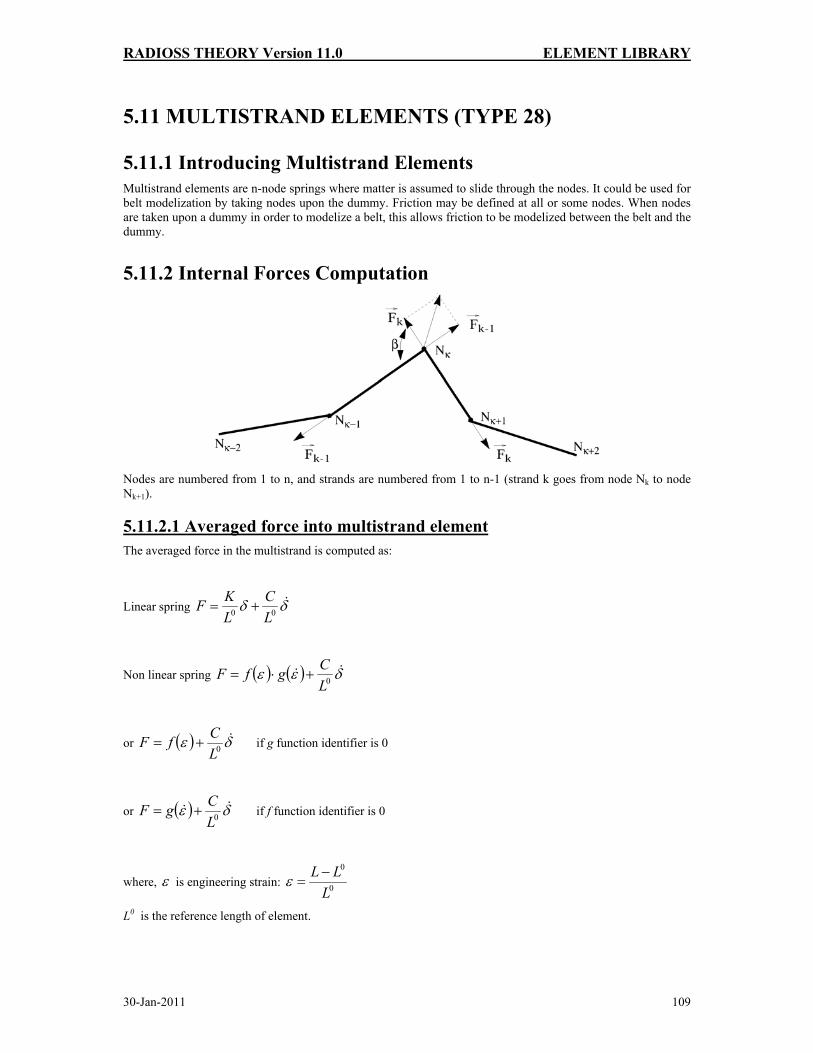
RADIOSS THEORY Version 11.0 ELEMENT LIBRARY
30-Jan-2011 109
5.11 MULTISTRAND ELEMENTS (TYPE 28)
5.11.1 Introducing Multistrand Elements Multistrand elements are n-node springs where matter is assumed to slide through the nodes. It could be used for belt modelization by taking nodes upon the dummy. Friction may be defined at all or some nodes. When nodes are taken upon a dummy in order to modelize a belt, this allows friction to be modelized between the belt and the dummy.
5.11.2 Internal Forces Computation
Nodes are numbered from 1 to n, and strands are numbered from 1 to n-1 (strand k goes from node Nk to node Nk+1).
5.11.2.1 Averaged force into multistrand element The averaged force in the multistrand is computed as:
Linear spring δδ &00 L
CLKF +=
Non linear spring ( ) ( ) δεε &&0L
CgfF +⋅=
or ( ) δε &0L
CfF += if g function identifier is 0
or ( ) δε &&0L
CgF += if f function identifier is 0
where, ε is engineering strain: 0
0
LLL −
=ε
L0 is the reference length of element.

RADIOSS THEORY Version 11.0 ELEMENT LIBRARY
30-Jan-2011 110
5.11.2.2 Force into each strand The force into each strand k is computed as:
Fk=F+ΔFk
ΔFk is computed an incremental way:
( ) ( ) δεδε 001LK
lKtFtF kk
kk −+−Δ=Δ EQ. 5.11.2.1
with 0kl the length of the unconstrained strand k, ( ) ( )1−−= tt εεδε and ( )kkkk vvtu −⋅= +1δδε ,
where ku is the unitary vector from node Nk to node Nk+1 .
Assuming:
00 LL
ll
k
k = EQ. 5.11.2.2
where kl is the actual length of strand k.
Therefore equation 5.11.2.1 reduces to:
( ) ( ) ⎟⎟⎠
⎞⎜⎜⎝
⎛−+−Δ=Δ δεδε
kkkk l
LlKtFtF 01 EQ. 5.11.2.3
5.11.2.3 Friction Friction is expressed at the nodes: if μ is the friction coefficient at node k, the pulley friction at node Nk is expressed as:
( ) ⎟⎠⎞
⎜⎝⎛Δ+Δ+≤Δ−Δ −− 2
tanh2 11βμ
kkkk FFFFF EQ. 5.11.2.4
When equation 5.11.2.4 is not satisfied, kk FF Δ−Δ −1 is reset to ( ) ⎟⎠⎞
⎜⎝⎛Δ+Δ+ − 2
tanh2 1βμ
kk FFF .
All the kFΔ (k=1,n-1) are modified in order to satisfy all conditions upon kk FF Δ−Δ −1 (k=2,n-1), plus the following condition on the force integral along the multistrand element:
( )∑−=
=Δ+1,1 nk
kk LFFFl EQ. 5.11.2.5
This process could fail to satisfy equation 5.11.2.4 after the )1,1( −=Δ nkFk modification, since no iteration is made. However, in such a case one would expect the friction condition to be satisfied after a few time steps.
NOTE: Friction expressed upon strands (giving a friction coefficient μ along strand k) is related to pulley friction by adding a friction coefficient μ /2 upon each nodes Nk and Nk+1 .

RADIOSS THEORY Version 11.0 ELEMENT LIBRARY
30-Jan-2011 111
5.11.2.4 Time step Stability of a multistrand element is expressed as:
kK
CKlCt
k
kkkk ∀−+
≤Δ ,2 ρ
EQ. 5.11.2.6
with 0LdmultistrantheofMassKk = and (assuming 9.2.2.2) :
( )⎟⎟⎠
⎞⎜⎜⎝
⎛−
=⎟⎟⎠
⎞⎜⎜⎝
⎛−
= 0000 ,max,maxLLl
FLLl
KLll
FlKK
kkkkkk EQ. 5.11.2.7
( ) ( )( ) ( ) 00 Ll
LCddgf
l
Cddgf
Ckk
k ⎟⎠⎞
⎜⎝⎛ +=
⎟⎠⎞
⎜⎝⎛ +
= εε
εε
εε
&
&&
EQ. 5.11.2.8
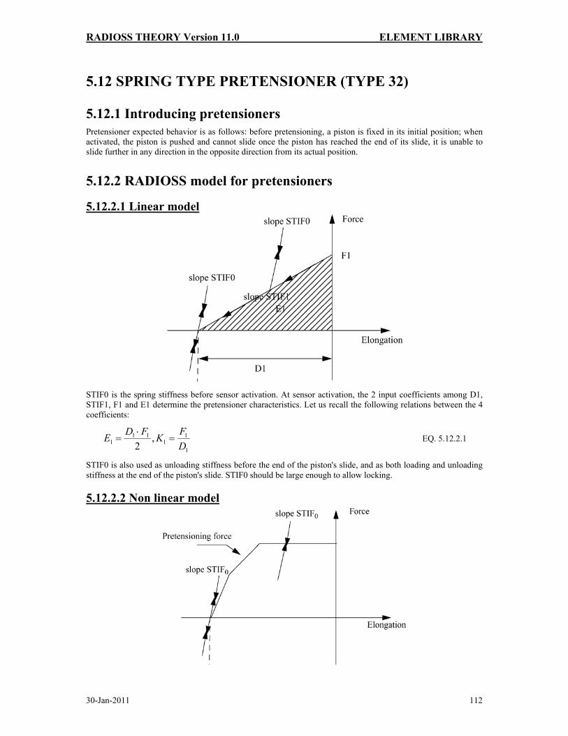
RADIOSS THEORY Version 11.0 ELEMENT LIBRARY
30-Jan-2011 112
5.12 SPRING TYPE PRETENSIONER (TYPE 32)
5.12.1 Introducing pretensioners Pretensioner expected behavior is as follows: before pretensioning, a piston is fixed in its initial position; when activated, the piston is pushed and cannot slide once the piston has reached the end of its slide, it is unable to slide further in any direction in the opposite direction from its actual position.
5.12.2 RADIOSS model for pretensioners
5.12.2.1 Linear model
STIF0 is the spring stiffness before sensor activation. At sensor activation, the 2 input coefficients among D1, STIF1, F1 and E1 determine the pretensioner characteristics. Let us recall the following relations between the 4 coefficients:
1
11
111 ,
2 DFKFDE =
⋅= EQ. 5.12.2.1
STIF0 is also used as unloading stiffness before the end of the piston's slide, and as both loading and unloading stiffness at the end of the piston's slide. STIF0 should be large enough to allow locking.
5.12.2.2 Non linear model

RADIOSS THEORY Version 11.0 ELEMENT LIBRARY
30-Jan-2011 113
STIF0 is spring stiffness before sensor activation. Depending on the input, pretensioning force is defined as f(L-L0), with either g(t-t0), or f(L-L0).g(t-t0), with L0 length of the spring at sensor activation time and at t0 sensor activation time.
Similar use of STIF0 allows piston locking.
5.12.2.3 Force computation Let the pretensioning force ( ) ( )( )011 LtLSTIFFtFp −⋅+= for a linear model,
and ( ) ( )( )0LtLftFp −= or ( )0ttg − or ( )( ) ( )00 ttgLtLf −⋅− for a non linear model.
The force into the pretensioner spring is computed as: EQ. 5.12.2.2
if, ( ) 0≥+ dttFp
( ) ( ) ( ) ( ) ( )( )tLdttLSTIFtFdttFMaxdttF p −+⋅++=+ 0,
and ( ) ( ) ( ) ( )( )tLdttLSTIFtFdttF −+⋅+=+ 0 otherwise.