Tetsuo Sasao and Andre B. FletcherIntroduction to VLBI SystemsChapter 2Lecture Notes for KVN StudentsPartly Based on Ajou University Lecture Notes(to be further edited)Version 1.Created on December 05, 2004.Revised on January 14, 2005.Revised on March 18, 2005.Revised on April 14, 2005.Revised on July 27, 2006.Revised on June 15, 2007.Revised on March 5, 2008.Revised on April 16, 2009.Revised on September 27, 2009.

Radio Telescope AntennasThis chapter describes principles and characteristics of antennas as very

important components of VLBI systems.

Contents

1 Antenna Overview 51.1 Antennas for VLBI . . . . . . . . . . . . . . . . . . . . . . . . 51.2 Classifications of Radio Telescope Antennas . . . . . . . . . . 6

1.2.1 Main Reflector Design . . . . . . . . . . . . . . . . . . 61.2.2 Mounting and Tracking Design . . . . . . . . . . . . . 61.2.3 Wheel & Track and Yoke & Tower Alt–Azimuth An-

tennas . . . . . . . . . . . . . . . . . . . . . . . . . . . 101.2.4 Stiffness . . . . . . . . . . . . . . . . . . . . . . . . . . 101.2.5 Antenna Reference Point . . . . . . . . . . . . . . . . . 111.2.6 Observing Frequency . . . . . . . . . . . . . . . . . . . 13

1.3 Basic Structure of a Paraboloidal Antenna . . . . . . . . . . . 161.4 Why Paraboloid? . . . . . . . . . . . . . . . . . . . . . . . . . 17

1

2 Antenna Beams 182.1 Some Elements of Vector Algebra . . . . . . . . . . . . . . . . 182.2 Electromagnetic Waves in a Free Space . . . . . . . . . . . . . 24

2.2.1 Maxwell Equations . . . . . . . . . . . . . . . . . . . . 242.2.2 Equation of Continuity . . . . . . . . . . . . . . . . . . 262.2.3 Conservation of Energy and Poynting Vector . . . . . . 262.2.4 Wave Equations in a Stationary Homogeneous Neutral

Medium . . . . . . . . . . . . . . . . . . . . . . . . . . 282.2.5 Monochromatic Plane Waves . . . . . . . . . . . . . . . 292.2.6 Electric and Magnetic Fields in a Plane Wave . . . . . 31

2.3 Generation of Electromagnetic Waves . . . . . . . . . . . . . . 352.3.1 Electromagnetic Potentials . . . . . . . . . . . . . . . . 352.3.2 Lorentz Gauge . . . . . . . . . . . . . . . . . . . . . . 362.3.3 Wave Equations with Source Terms . . . . . . . . . . . 372.3.4 Solution of the Wave Equation with the Source Term . 392.3.5 Retarded Potential . . . . . . . . . . . . . . . . . . . . 432.3.6 Transmission of Radio Wave from a Harmonically Os-

cillating Source . . . . . . . . . . . . . . . . . . . . . . 452.3.7 Electromagnetic Fields Far from the Source Region . . 462.3.8 Far Field Solution and Fraunhofer Region . . . . . . . 482.3.9 Hertz Dipole . . . . . . . . . . . . . . . . . . . . . . . . 512.3.10 Linear Dipole Antenna of Finite Length . . . . . . . . 53

2.4 Transmitting and Receiving Antennas . . . . . . . . . . . . . . 572.4.1 The Reciprocity Theorem . . . . . . . . . . . . . . . . 572.4.2 Equivalence of Field Patterns in Transmission and Re-

ception . . . . . . . . . . . . . . . . . . . . . . . . . . . 602.5 Transmission from Aperture Plane . . . . . . . . . . . . . . . 62

2.5.1 Aperture Antennas . . . . . . . . . . . . . . . . . . . . 622.5.2 Boundary Conditions on the Aperture Plane

“Magnetic Current” and “Magnetic Charge” . . . . . . 642.5.3 Wave Equations with Magnetic Current and Magnetic

Charge . . . . . . . . . . . . . . . . . . . . . . . . . . . 672.5.4 Radio Wave Transmission from a Surface . . . . . . . . 692.5.5 Radio Wave Transmission from an Aperture Antenna . 722.5.6 Aperture Illumination and Field Pattern of an Aper-

ture Antenna . . . . . . . . . . . . . . . . . . . . . . . 742.5.7 Power Pattern of an Aperture Antenna . . . . . . . . . 752.5.8 Main Lobe, Sidelobes, HPBW and BWFN . . . . . . . 762.5.9 Uniformly Illuminated Rectangular Aperture Antenna . 772.5.10 Circular Aperture Antenna . . . . . . . . . . . . . . . . 78

2.6 Beam Patters of Aperture Antennas . . . . . . . . . . . . . . . 83

2

2.6.1 Antenna–Fixed Coordinate System . . . . . . . . . . . 832.6.2 A Useful Formula: HPBW ≈ λ/D . . . . . . . . . . . . 842.6.3 Distance to Fraunhofer Region . . . . . . . . . . . . . . 84

2.7 Illumination Taper (or Gradation) . . . . . . . . . . . . . . . . 872.8 Spectral Flux Density Received by an Antenna Beam . . . . . 90

3 Antenna Characteristics 913.1 Directive Gain G(θ, φ) . . . . . . . . . . . . . . . . . . . . . . 943.2 Beam Solid Angle ΩA . . . . . . . . . . . . . . . . . . . . . . . 953.3 Main Beam Solid Angle ΩM . . . . . . . . . . . . . . . . . . . 953.4 Main Beam Efficiency ηM . . . . . . . . . . . . . . . . . . . . 963.5 Directivity, Maximum Directive Gain, or “Gain” D . . . . . . 963.6 Antenna Polarization . . . . . . . . . . . . . . . . . . . . . . . 97

3.6.1 Some Notes on Polarization of Electromagnetic Wave . 973.6.2 Polarization Characteristics of Antennas . . . . . . . . 973.6.3 Antenna Polarization and VLBI . . . . . . . . . . . . . 99

3.7 Effective Aperture Ae . . . . . . . . . . . . . . . . . . . . . . . 993.8 Aperture Efficiency ηA . . . . . . . . . . . . . . . . . . . . . . 1003.9 Nyquist Theorem on Noise Power . . . . . . . . . . . . . . . . 1013.10 Effective Aperture and Beam Solid Angle . . . . . . . . . . . . 1033.11 Directivity D and Aperture Efficiency ηA . . . . . . . . . . . . 1053.12 Illumination Taper and Aperture Efficiency . . . . . . . . . . . 1063.13 Surface Roughness and Aperture Efficiency . . . . . . . . . . . 1063.14 Surface Accuracy and Lower Limit of the Observing Wavelength1093.15 Pointing Accuracy . . . . . . . . . . . . . . . . . . . . . . . . 1143.16 Design of the Feed System . . . . . . . . . . . . . . . . . . . . 1173.17 Visible Reference Point . . . . . . . . . . . . . . . . . . . . . . 1233.18 Alignment Errors and Offset of Axes . . . . . . . . . . . . . . 1233.19 Range of Motion . . . . . . . . . . . . . . . . . . . . . . . . . 1243.20 Slewing Speed . . . . . . . . . . . . . . . . . . . . . . . . . . . 1253.21 Operational and Survival Loads . . . . . . . . . . . . . . . . . 125

4 Antenna Temperature and Single Dish Imaging 1264.1 What Is the Antenna Temperature TA? . . . . . . . . . . . . . 1264.2 Imaging with the Single Dish Radio Telescope . . . . . . . . . 128

5 Receiving Systems 1305.1 System Noise Temperature . . . . . . . . . . . . . . . . . . . . 131

5.1.1 The “Input Equivalent Noise” . . . . . . . . . . . . . . 1315.1.2 Signal Attenuation and Thermal Noise . . . . . . . . . 132

3

5.1.3 System Noise Temperature of the Multistage ReceivingSystem . . . . . . . . . . . . . . . . . . . . . . . . . . . 135

5.1.4 Receiver Noise Temperature TRX . . . . . . . . . . . . 1375.1.5 Antenna Noise Temperature Tant and Atmospheric Con-

tribution to the System Noise Temperature . . . . . . . 1405.2 Frequency Conversion . . . . . . . . . . . . . . . . . . . . . . . 143

5.2.1 Technical Terms in the Frequency Conversion . . . . . 1445.2.2 What Is the Mixer? . . . . . . . . . . . . . . . . . . . . 1455.2.3 Upper Sideband (USB) and Lower Sideband (LSB) . . 1465.2.4 Sideband Rejection . . . . . . . . . . . . . . . . . . . . 147

5.3 Signal–to–Noise Ratio of the Single–Dish Radio Telescope . . . 1495.4 Gain Variation of Receivers and Switching Observations . . . . 153

5.4.1 Dicke Mode Switching Observation . . . . . . . . . . . 1545.4.2 Beam Switch . . . . . . . . . . . . . . . . . . . . . . . 1565.4.3 Additional Remarks on Switching Mode Observations . 158

6 Measurements of Antenna Performance 1586.1 System Equivalent Flux Debsity (SEFD) . . . . . . . . . . . . 1596.2 Measurement of the Receiver Noise Temperature TRX . . . . . 1606.3 Measurement of the System Noise Temperature . . . . . . . . 1616.4 System Noise Temperature and Antenna Temperature Re-

ferred to the Outside of the Atmosphere T ⋆S and T ⋆

A . . . . . . 1636.5 Measurement of the TS⋆ . . . . . . . . . . . . . . . . . . . . . 1646.6 Measurement of the Aperture Efficiency ηA . . . . . . . . . . . 1656.7 Chopper Wheel method for Precise Measurement of the An-

tenna Temperature T ⋆A . . . . . . . . . . . . . . . . . . . . . . 166

6.8 Measurement of the Optical Depth of the Atmosphere τatm —sec z Method . . . . . . . . . . . . . . . . . . . . . . . . . . . 167

6.9 Pointing Calibration and Pointing Accuracy σθ . . . . . . . . . 1716.9.1 Pointing Model . . . . . . . . . . . . . . . . . . . . . . 1716.9.2 Pointing Measurement . . . . . . . . . . . . . . . . . . 176

6.10 Beam Pattern Measurement . . . . . . . . . . . . . . . . . . . 179

4

1 Antenna Overview

According to J.D. Kraus, the antenna is ‘a region between a guided waveand a free–space wave or vice versa’ and ‘the antenna interfaces electrons onconductors and photons in space’ (see Figure 1). In addition, he says that‘the eye is another such device’ (J.D. Kraus, Electromagnetics, 3rd Edition,1984).

Figure 1: What is an antenna? (From Kraus, 1984).

1.1 Antennas for VLBI

Antennas are quite important components of VLBI (Very Long Baseline In-terferometry), because

• They are the most expensive devices in VLBI.Usually antennas are more than an order of magnitude more expen-sive than receivers, data acquisition systems, frequency standards, andrecorders.

5

• Data quality is sensitive to antennas.Characteristics of antennas, such as sensitivity, pointing, cross-polarization,gravitational and thermal deformation, and so on, directly affect qual-ity of results of astrophysical and geodetic VLBI observations.

• It is difficult to repair or replace antennas.We have to stop observations for months, and pay very much money,to do so.

Therefore, we must have a good knowledge about antennas, and must doour best in designing and constructing antennas for making a good VLBIsystem.

1.2 Classifications of Radio Telescope Antennas

In the early history of radio astronomy, a variety of antennas, like dipoleantennas or horn antennas, were used. However, the overwhelming majorityof radio telescopes nowadays adopt the design of the paraboloidal (or, inexceptional cases, spherical) filled aperture antennas.

Existing radio telescope antennas may be classified into subgroups, ac-cording to several points of view.

1.2.1 Main Reflector Design

The rotationally symmetric paraboloidal shape is the most widely used indesigns of main reflectors. The 100 m telescope at Effelsberg, Germany, isan example (see Figure 2).

The new Greenbank 100 m telescope (GBT), USA, adopts the offsetparaboloidal design in order to achieve maximum efficiency in the receptionof radio waves (see Figure 3).

In several huge radio telescopes in the world, partial paraboloidal surfacesare used in a cylindrical paraboloid design. The RATAN–600 telescope inRussia is an example (see Figure 4).

1.2.2 Mounting and Tracking Design

The most frequently used design for radio telescope mounting is the Alt–Azimuth design, which has a vertical azimuthal axis, and a horizontal alti-tude axis. The Alt–Azimuth mount (or ‘Az–El mount’ as frequently referredto by radio astronomers) is most symmetrical with respect to the direction

6

Figure 2: Effelsberg 100 m paraboloidal radio telescope, Germany.

Figure 3: The giant offset paraboloid telescope GBT, USA.

Figure 4: The partial cylindrical paraboloid antenna RATAN–600, Russia.

7

of gravity, and hence is suited to the stable support of a large and heavy an-tenna structure. On the other hand, for tracking the diurnal motion of a radiosource, real–time coordinate transformation from celestial equatorial (rightascention and declination) coordinates to horizontal (azimuth and elevation)coordinates, and simultaneous driving of the antenna around the two axes,are always required in this mount system. Moreover, it is in general difficultfor an Alt–Azimuth telescope to track sources around the zenith direction.One of the 20 m antennas of the VERA (VLBI Exploration of Radio As-trometry) array at Iriki, Japan, is shown as an example of the Alt–Azimuthradio telescope (left panel in Figure 5).

The most popular mounting design for optical telescopes, except for re-cent huge ones, the Equatorial mount, has a polar axis parallel to the rotationaxis of the Earth, and a declination axis. The Equatorial mount is suitedfor easy tracking of radio sources in any direction in the sky, and is usedfor relatively light–weight radio telescopes. The 25 m antennas in the West-erbork Synthesis Radio Telescope (WSRT, the Netherlands) are examples(right panel in Figure 5).

Figure 5: Alt–Azimuth mount antenna at the VERA Iriki station, Japan (Left), andEquatorial mount antennas in the WSRT, the Netherlands (Right).

In general, for orienting an antenna towards a desired sky position, weneed an axis fixed with respect to the ground, which we call “fixed axis”, andanother axis rotating around the fixed axis, which we call “moving axis”. Inthe Alt–Azimuth design, the fixed axis is the azimuthal axis, and the movingaxis is the elevation axis. In the Equatorial design, the fixed axis is the polaraxis, and the moving axis is the declination axis.

A little unusual XY mount design, with a horizontal fixed axis, is adoptedin 26 m antenna at Hobart, University of Tasmania, Australia (Figure 6).This antenna was originally built by NASA for tracking space vehicles, and

8

Figure 6: XY mount antenna at Hobart, Australia.

was installed near Canberra. Later, the antenna was moved to Hobart, andnow is intensively used for geodetic and astrophysical VLBI observations.

A very unique design consisting of a fixed spherical main reflector antennais used in the giant 305 m radio telescope at Arecibo (Puerto Rico, USA).Instead of driving the main reflector, a cable suspended subreflector withspecial aberration correction optics is driven to track the radio source (seeFigure 7).

Figure 7: A spherical fixed main reflector antenna at Arecibo, Puerto Rico, USA, 305m diameter.

9

1.2.3 Wheel & Track and Yoke & Tower Alt–Azimuth Antennas

Figure 8 shows the 20 m VERA antenna (Left), and the 10 m antenna(Right), in NAO Mizusawa, Japan.

The entire structure of the 20 m antenna is supported by four wheels,which move on a circular rail fixed on the antenna foundation, in order tochange the azimuthal orientation of the antenna. Such an antenna is calleda “wheel & track” antenna.

Figure 8: Wheel & Track (left) and Yoke & Tower (Right) antennas.

In the 10 m antenna, an azimuth gear is attached to the top of the tower–like pedestal, and the antenna structure above the gear is rotated around theazimuth axis by the motor drives. Such an antenna is called “yoke & tower”antenna.

Generally, the yoke & tower design is suited to keep a fixed intersectionpoint for the Azimuth and Elevation axes – this is an important referencepoint in geodetic VLBI. However, for mechanical reasons, the wheel & trackdesign is more frequently used for large aperture antennas.

1.2.4 Stiffness

For some large aperture millimeter wave telescopes aimed mainly at spec-troscopy and imaging of radio sources, a flexible structure is adopted torealize the so–called “homologous transformation”, which is such that thedeformed main reflector surface maintains a paraboloid shape, and forms asharp focus, even when the telescope is tilted under the action of the Earth’s

10

Figure 9: A flexible 45 m Millimeter–Wave Telescope at Nobeyama, Japan (left), and a“stiff” 32 m geodetic VLBI antenna at Tsukuba, Japan (Right).

gravity. The 45 m Millimeter–Wave Telescope at Nobeyama, Japan, is asuccessful example of such a design (see left panel in Figure 9).

On the other hand, radio telescope antennas for geodetic and astrometricVLBI observations are usually designed to be very stiff, to eliminate possibleerrors due to the deformation of the telescope. The 32 m geodetic VLBIantenna at Tsukuba, Japan, is an example of the “stiff” telescope (rightpanel in Figure 9).

1.2.5 Antenna Reference Point

Geodetic VLBI determines positions of reference points of antennas withtypical accuracy of 1 cm or better. Therefore, it is very important to preciselydefine and maintain the reference points in the antennas.

In general, we can select any point in an antenna as a reference point,as far as the point is fixed with respect to the ground. There are certainpreferable points, however, suitable to the geodetic analysis.

The best choice is the cross point of fixed and moving axes of the antenna,when the two axes intersect. In such a case, difference between a time tr,when a wave front from an astronomical radio source crosses the referencepoint, and a time tf , when a part of the same wave front, which is reflectedby main– and subreflectors and then transmitted via a cable, reaches to apoint where a time tag is added to the signal, is constant (i.e. tf − tr =const) irrespective of a sky direction of the source, as far as time variationsof antenna structure and receiver–transmission characteristics can be ignoredor well calibrated. This is really comvenient for geodetic VLBI analysis sincewe can then assume that an observed delay between two stations A and Bwhich is τobs = tfB

− tfAis equal to a delay between arrival times of a same

wave front at reference points of two antennas τref = trB−trA

plus a constant

11

term (i.e. τobs = τref+ const).If the two axes do not intersect, we usually choose a point in the fixed axis

closest to the moving axis and add a source–direction dependent correctionterm to the relation between τobs and τref .

Figure 10: Alt–Azimuth mount 11 m antenna at Kashima, Japan (left), and Equatorialmount 43 m antenna at Green Bank, USA (Right). Locations of fixed and moving axesare schematically shown by straight lines.

In Alt–Azimuth mount antennas, the fixed azimuth axis and moving el-evation axis are usually designed to intersect with each other. An exampleis 11 m antenna at Kashima, Japan (left panel in Figure 10). In Equatorialmount antennas, it is usually difficult to make the right–ascension and dec-lination axes to intersect with each other. An example is 43 m antenna inGreen Bank, USA (right panel in Figure 10).

Figure 11: 11 m antenna at Kashima, Japan, with the reference point directly visiblefrom outside (Left), and 32 m antenna at Tsukuba, Japan, with the reference point invisiblefrom outside (Middle). Also shown is a cat’s eye used in ground geodetic measurements.

It is very important for geodetic VLBI to tie the antenna reference point

12

with geodetic markers on the ground, in order, for example, to combinea national geodetic network with the VLBI–based international frame. For

Figure 12: In 20 m geodetic VLBI antenna (Top, Left) at Wettzell, Germany, a compactreceiver room is located in the back structure of the main reflector, and the Az–El crosspoint is covered by a cabin fixed on a rotating disk above the azimuth gear (Top, Middle).There is a firmly supported meausrement bench in the cabin (Bottom, Middle). Verticaldisplacement of the bench is accurately monitored with respect to the invar tube which isfixed to the ground and vertically extended along the Az–axis (Bottom, Left). The targeton the bench (Right) is adjusted to the right cross–point of the two axes, and is measuredfrom geodetic markers on the ground through a hatch of the cabin (Top, Midle).

this purpose, we conduct ground geodetic measurement of the position of thereference point with respect to the geodetic markers, using special devicessuch as “cat’s eye” (rightmost panel of Figure 11). It is very convenient insuch measurements if the position of the reference point is directly “visible”from outside where we can place a cat’s eye. Figure 11 shows examples ofAlt–Azimuth antennas with visible and invisible reference points.

A geodetic VLBI antenna with 20 m diameter in Wettzell Fundamen-tal Station, Germany, is specially designed for precise measurements of thereference point (Figure 12).

1.2.6 Observing Frequency

The most significant factor in antenna design today is the maximum fre-quency of observation. Antennas are often called as “cm–wave–”, “mm–wave–” or “submm-wave” antennas, according to their maximum observingfrequency (or shortest observing wavelength). In order to convert wavelengthλ to frequency ν, one can use a convenient approximate formula:

ν (in GHz) ≃ 30

λ (in cm). (1)

13

For cm–wave antennas, the requirements of surface and pointing accuracyare not very severe for present–day antenna manufacturing technology. It istherefore relatively easy to make large antennas in the cm–wave range. At thelow–frequency end, the main reflectors of cm–wave antennas can be made ofmeshed wires. The 25.6 m antenna at Onsala, Sweden, is an example (Figure13).

Figure 13: A cm–wave antenna at Onsala, Sweden, 25.6 m diameter.

For mm–wave antennas, the surface accuracy must be as small as 0.1 mmrms, and the pointing accuracy must be as good as 0.001 degree rms. Thelarge aperture mm–wave antennas like the IRAM 30 m (Spain, EU; left panelin Figure 14), the Nobeyama 45 m (left panel in Figure 9), and the Effelsberg100 m (Figure 2) are the result of state–of–the–art achievements of moderntechnology. Some of the mm–wave telescopes, including the TRAO 14 mtelescope at Daejeon, Korea (see right panel in Figure 14), are covered byradomes to avoid the effects of strong wind and inhomogeneous solar heating.

The most stringent tolerances in antenna construction are required inthe submm–wave range. As a result, all existing submm–wave antennas arerelatively small (with diameters around 10 m or smaller), and some of themare located within domes, just like the big optical telescopes. Since theatmosphere is largely opaque in the submm–wave range at low altitude sitesnear sea level, but fairly transparent at dry high altitude sites, submm–wavetelescopes are built on high moutains, with altitudes of 3000–5000 m abovesea level (see Figures 15 and 16).

14

Figure 14: IRAM mm–wave telescope, Spain, 30 m diameter (Left), and radome–coveredTRAO 14 m mm–wave telescope at Daejeon, Korea (Right).

Figure 15: The largest submm–wave antenna JCMT, UK, 15 m diameter, at MaunaKea, Hawaii.

Figure 16: Main reflector (Left) and radome (Right) of the 1.2 m submm–wave telescopewhich worked for several years at the Top of Mount Fuji, Japan.

15

1.3 Basic Structure of a Paraboloidal Antenna

The basic components of the structure of an Alt–Azimuth paraboloidal an-tenna are shown in Figure 17. The paraboloidal structure is rotated around

subreflector

stay

main reflector

panel support

back structure

center hub

El limit

El drive motor

step

cable wrap

feed horn

s-band feed

feed cover

Az axis

El axisreceiver room

El cable wrap

supportstructurecounter weight

compressor

Az bearing

joint plate

& bearing

Az drive motor

El gear

Az gear

Figure 17: Structure of 10 m VLBI antenna at NAO Mizusawa, Japan.

the fixed vertical Azimuth axis, and the horizontal Elevation axis, in orderto point to any direction in the sky. Usually, the main reflector is composedof a number of panels made of aluminum or carbon fiber, etc, which are fixedto the back structure by adjustable supports. The feed horn is a kind ofsmall antenna, and there is a so–called waveguide to coaxial–cable (orcoaxial to waveguide) converter at the neck of the feed horn, where theelectromagnetic field in space generates the voltage in circuits or vice versa.The waveguide to coaxial–cable converter is the only “real antenna” in strictsense of the second definition of the antenna by Kraus: ‘the antenna inter-faces electrons on conductors and photons in space’. The huge structuressuch as the main reflectors and subreflectors, can be regarded as auxilliaryreflecting devices.

16

1.4 Why Paraboloid?

Why are paraboloidal antennas the most frequently used for radio telescopes?This is because paraboloids collect plane radio waves coming from astro-nomical sources towards a focal point where we can place the waveguide tocoaxial–cable converter, which transforms the energy of photons in free spaceto the energy of electrons in conductors in the most efficient way.

a

b

a

b

c

Figure 18: Primary (Left) and secondary (Right) foci of paraboloidal antennas.

In the secondary focus system shown in the right panel of Figure 18, acombination of a paraboloidal main reflector and a hyperboloidal subreflectorproduces the secondary focus near the main reflector, where the receivers canbe conveniently placed. The path length of a ray from the aperture plane —shown by dotted horizontal lines in Figure 18 — to the focus is a + b in theprimary focus system, and a+b+c in the secondary focus system; this lengthis kept constant for any ray coming parallel with the symmetry axis of theparaboloid. Therefore, the radio waves are collected and summed up withequal phases (i.e. in a “phase–coherent” way) at the foci of the paraboloidalantennas.

There are two possible designs for forming the secondary focus in paraboloidalantennas which use convex (Cassegrain) and concave (Gregorian) hyper-boloidal mirrors, respectively, as subreflectors (Figure 19).

The Cassegrain design is widely adopted in radio telescopes, because itallows a relatively stable structure against gravitational deformation andwind pressure. On the other hand, the Gregorian design is better suited tothe cases where both the primary and secondary foci are used for receivingdifferent frequency bands. In fact, in the Gregorian design, the primary focusfeed horn can simply be inserted in front of the subreflector when needed andthen removed to allow the secondary focus to be formed.

17

Figure 19: Cassegrain (Left) and Gregorian (Right) foci of paraboloidal antennas.

2 Antenna Beams

2.1 Some Elements of Vector Algebra

Many textbooks list formulae of vector algebra such as shown in Figure 20.It is not easy to memorize all these complicated formulae. Moreover, theymay often contain typographic errors! Without knowledge of these formulae,however, it is difficult to understand electromagnetic theory of radiotelescopeantennas.

Fortunately, it is not necessary at all to memorize all these formulae.Instead, we have to memorize just two symbols and one formula, only. Theyare the Kronecker symbol δij , the Levi–Civita symbol ǫijk, and a formulaǫijkǫilm = δjlδkm − δjmδkl. Here, repeated indecies i implies summation, aswe will see below.

Let us consider a rectangular (Cartesian) coordinate system, with basisvectors i1, i2, and i3, in a three–dimensional Euclidean space (Figure 21).

In this coordinate system, we consider a radius vector r with elements (orcomponents) x1, x2, and x3 drawn from the origin of the coordinate systemto a point with coordinates x1, x2, and x3. We consider also a scalar fieldΦ(r) and a vector field A(r) with elements A1, A2, and A3, as functions ofr.

Now let us introduce following notations and conventions.

1. Kronecker’s delta symbol δij

18

Figure 20: Typical formulae of vector algebra.

19

i2

i3

i1

x1

x2

x3

r

A(r)

Φ(r)

o

Figure 21: Rectangular coordinate system in a three–dimensional space.

δij is 1 when the two indecies take the same value, and 0when they are different.

δij =

0 at i 6= j

1 at i = j(with i, j = 1, 2, 3). (2)

Therefore, δ11 = δ22 = δ33 = 1, and δ12 = δ13 = · · · = δ32 = 0.

2. Levi–Civita’s anti–symmetric symbol ǫijk

ǫ123 is defined to be 1, and sign is changed whenever adjacentindecies are substituted.

ǫ123 = 1

ǫ213 = −ǫ123 = −1,

ǫ312 = −ǫ132 = ǫ123 = 1,

ǫ321 = −ǫ231 = ǫ213 = −ǫ123 = −1,

ǫ112 = −ǫ112 = 0, ǫ232 = −ǫ232 = 0,

· · · .

(3)

3. Einstein’s summation convention

Repeated indecies, ii say, imply summation over 11, 22 and

20

33. For example,

AiBi ≡3

∑

i=1

AiBi = A1B1 + A2B2 + A3B3,

and

Cjj ≡3

∑

i=1

Cii = C11 + C22 + C33.

(4)

4. Nabla symbol of spatial derivative ∇

∇ is a vector like differential operator with three ‘elements’

∂

∂x1

,∂

∂x2

, and∂

∂x3

, (5)

where ∂∂xi

stands for a partial derivative with respect to xi.

If we apply the above symbols and notations to vector fields A(r) andB(r), as well as to a scalar field Φ(r), we can express:

• a scalar (or inner) product A · B as

A · B = AiBi, (6)

• i–th element of a vector (or outer) product A × B as

(A × B)i = ǫijkAjBk, (7)

in fact, ǫ1jkAjBk = A2B3 − A3B2, ǫ2jkAjBk = A3B1 − A1B3, andǫ3jkAjBk = A1B2−A2B1, in agreement with the definition of the vectorproduct,

• i–th element of a gradient gradΦ as

(gradΦ)i = (∇Φ)i =∂

∂xi

Φ =∂Φ

∂xi

, (8)

• a divergence divA as

divA = ∇ · A =∂

∂xiAi =

∂Ai

∂xi, (9)

and

21

• i–th element of a rotation (or curl) rotA as

(rotA)i = (∇× A)i = ǫijk∂

∂xjAk = ǫijk

∂Ak

∂xj. (10)

A very useful relationship is known between the Levi–Civita’s and Kro-necker’s symbols, which is described by the formula mentioned earlier:

ǫijkǫilm = δjlδkm − δjmδkl. (11)

We can verify this formula by examining all possible combinations of indecies.In view of Einstein’s summation convention, equation (11) is equivalent

toǫ1jkǫ1lm + ǫ2jkǫ2lm + ǫ3jkǫ3lm = δjlδkm − δjmδkl. (12)

Since j, k, l and m may be 1, 2 or 3, equation (11) or (12) has, in general,34 = 81 components. However, symmetry conditions greately reduce numberof components which we really have to individually consider.

First, let us consider what happens if we substitute indecies j and k, orl and m. Because of the antisymmetric property of Levi–Civita symbol, theLHS of equation (11) is antisymmetric (only sign is changed) with respect tosuch a substitution, and the RHS is also antisymmetric, since if we substitutej and k, for example, the RHS changes its sign as:

δklδjm − δkmδjl = −(δjlδkm − δjmδkl).

This says that, if we prove equation (11) for jk or lm, then the equationis automatically proven for kj or ml. Moreover, if j = k or l = m, theboth sides must be equal to 0 (therefore, equal to each other), since for anynumber A, if A = −A, then A = 0. Consequently, among 9 components ofjk and 9 components of lm, we have to individually consider only 3 and 3components, which are ‘12’, ‘13’ and ‘23’, for example (see equation (13)).

jk =

11 12 13

21 22 23

31 32 33

, and lm =

11 12 13

21 22 23

31 32 33

. (13)

Hence, in total, 3×3 = 9 components were left to be individually considered.Furthermore, it can be easily seen that if l or m in equation (11) is not

equal to neither j nor k, then both sides must be equal to 0. In fact, if jk is‘12’, for example, equation (12) becomes

ǫ312ǫ3lm = δ1lδ2m − δ1mδ2l.

22

Both sides of this equation are equal to 0, if l or m is 3.So, we have to consider individually, only three cases when both jk and

lm = ‘12’, both jk and lm = ‘13’, and both jk and lm = ‘23’. They are

for ‘12′, LHS = ǫ312ǫ312 = 1, and RHS = δ11δ22 = 1,

for ‘13′, LHS = ǫ213ǫ213 = 1, and RHS = δ11δ33 = 1,

for ‘23′, LHS = ǫ123ǫ123 = 1, and RHS = δ22δ33 = 1.

Thus, we proved equation (11).

If we use the above symbols and equation (11), all the complicated for-mulae of vector algebra are derived in straight forward ways. For example,

[A × (B × C)]i = ǫijkAjǫklmBlCm

= ǫkijǫklmAjBlCm = (δilδjm − δimδjl)AjBlCm

= AjBiCj − AjBjCi = BiAjCj − CiAjBj

= [B(A · C) − C(A · B)]i,

and, therefore,

A × (B × C) = B(A · C) − C(A · B). (14)

We used here a property of Kronecker’s symbol: δijAj = Ai.

Also,

(A × B) · (C × D) = ǫijkǫilmAjBkClDm = AjBkCjDk − AjBkCkDj,

and, hence

(A × B) · (C × D) = (A · C)(B · D) − (A · D)(B · C). (15)

Furthermore,

[∇× (∇× A)]i = ǫijk∂

∂xjǫklm

∂∂xlAm

= (δilδjm − δimδjl)∂

∂xj

∂∂xlAm = ∂

∂xj

∂∂xiAj − ∂

∂xj

∂∂xjAi

= [∇(∇ · A) −∇2A]i,

where

∇2 ≡ ∂2

∂x21

+∂2

∂x22

+∂2

∂x31

,

23

and, therefore,∇× (∇× A) = ∇(∇ · A) −∇2A. (16)

Other useful examples are:

∇ · (A × B) =∂

∂xi

ǫijk(AjBk) = Bkǫkij∂

∂xi

Aj − Ajǫjik∂

∂xi

Bk, ⇒

∇ · (A × B) = B · (∇× A) − A · (∇× B), (17)

[∇× (∇Φ)]i = ǫijk∂

∂xj

∂

∂xkΦ = ǫikj

∂

∂xk

∂

∂xjΦ = −ǫijk

∂

∂xj

∂

∂xkΦ = 0, ⇒

rot(gradΦ) = ∇× (∇Φ) = 0, (18)

∇ · (∇× A) =∂

∂xiǫijk

∂

∂xjAk = ǫijk

∂

∂xi

∂

∂xjAk = 0, ⇒

div(rotA) = ∇ · (∇× A) = 0, (19)

and,

∇ · (ΦA) =∂

∂xi(ΦAi) =

∂Φ

∂xiAi + Φ

∂Ai

∂xi= ∇Φ · A + Φ∇ · A, ⇒

div(ΦA) = gradΦ · A + Φ divA. (20)

2.2 Electromagnetic Waves in a Free Space

Prior to considering receptions and transmissions of radio waves (or, moregenerally speaking, electromagnetic waves) by antennas , we will briefly dis-cuss general behaviors of the electromagnetic waves in a free space, based onthe classical theory of electromagnetic fields.

2.2.1 Maxwell Equations

Let us consider following vector and scalar field quantities:

24

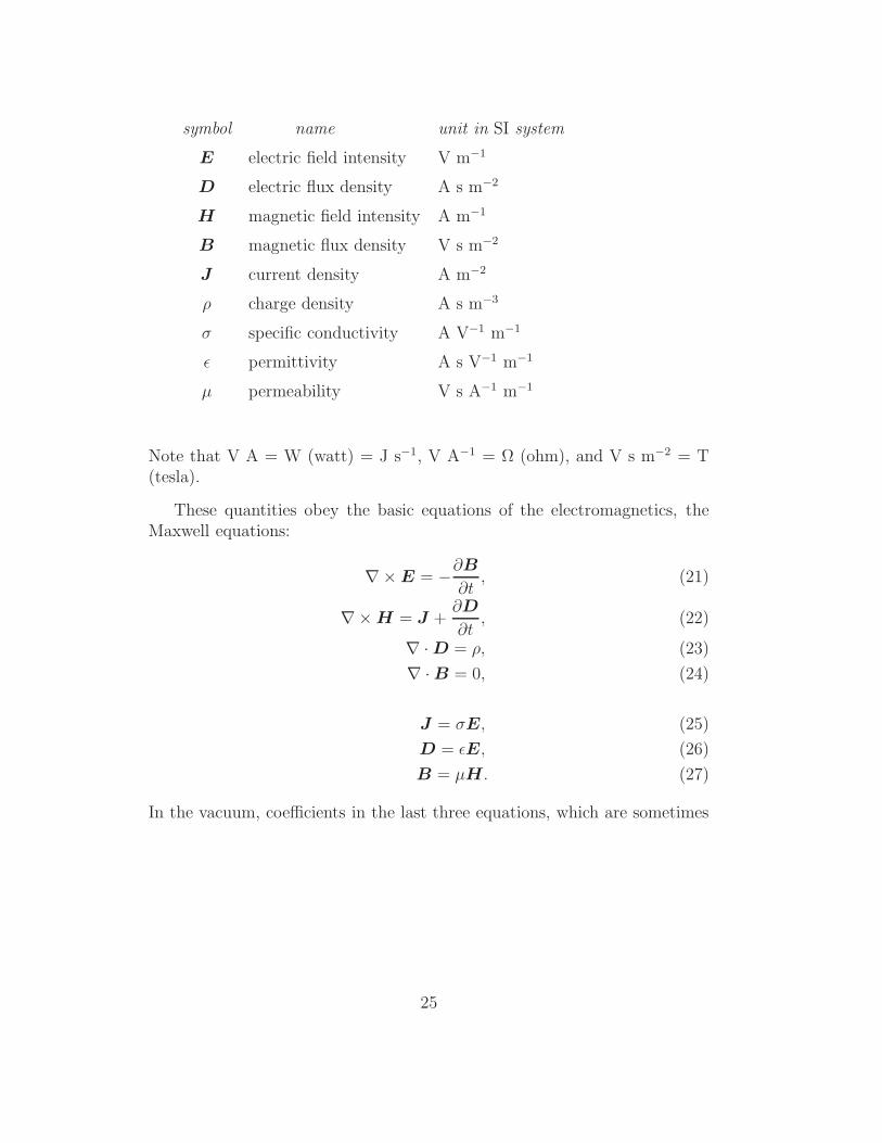
symbol name unit in SI system

E electric field intensity V m−1

D electric flux density A s m−2

H magnetic field intensity A m−1

B magnetic flux density V s m−2

J current density A m−2

ρ charge density A s m−3

σ specific conductivity A V−1 m−1

ǫ permittivity A s V−1 m−1

µ permeability V s A−1 m−1

Note that V A = W (watt) = J s−1, V A−1 = Ω (ohm), and V s m−2 = T(tesla).

These quantities obey the basic equations of the electromagnetics, theMaxwell equations:

∇× E = −∂B∂t

, (21)

∇× H = J +∂D

∂t, (22)

∇ · D = ρ, (23)

∇ · B = 0, (24)

J = σE, (25)

D = ǫE, (26)

B = µH. (27)

In the vacuum, coefficients in the last three equations, which are sometimes

25

called as ‘equations of state’, take following values:

σ0 = 0,

ǫ0 = 8.854 × 10−12 A s V−1 m−1,

µ0 = 1.257 × 10−6 V s A−1 m−1,

which satisfy

ǫ0µ0 = c−20 ,

(28)

where suffix 0 implies a vacuum value, and c0 = 2.998×108 m s−1 is the lightvelocity in the vacuum.

2.2.2 Equation of Continuity

From Maxwell equations (22) and (23), and a formula of vector algebra givenin equation (19), we obtain

∂ρ

∂t+ ∇ · J = 0. (29)

This equation implies that time variation of the electric charge, containedwithin a finite region, is eqaul to the electric current flowing into (or flowingout of) the region within a unit time. Therefore, this equation is called ‘equa-tion of continuity of electric charge’ or ’equation of conservation of electriccharge’.

2.2.3 Conservation of Energy and Poynting Vector

If we take scalar products of equations (21) and (22) with −H and E, re-spectively, and sum them up, we obtain

E · ∂D∂t

+ H · ∂B∂t

= −E · J + E · (∇× H) − H · (∇× E)

= −E · J −∇ · (E × H), (30)

where we used a formula of vector algebra given in equation (17).Considering equations (25), (26), and (27), and assuming that permittiv-

ity ǫ and permeability µ are constant in time, we can express equation (30)in a form:

1

2

∂(E · D + H · B)

∂t+ ∇ · (E × H) = −σE2. (31)

Then, taking into account that

26

1. u ≡ 12(E ·D +H ·B) is the energy density of the electromagnetic field

[J m−3],

2. S ≡ E × H is the energy flux of the electromagnetic field, called‘Poynting vector’ [W m−2],

3. −σE2 is the Joule heat generated per unit time and unit volume dueto the Ohmic dissipation [W m−3],

we can interpret equation (31) as an equation of conservation of eletromag-netic energy (Figure 22):

∂u

∂t+ ∇ · S = −σE2. (32)

u=1_2

(ED+HB)

S=ExH

-σE2

Figure 22: Energy conservation of electromagnetic energy.

Among the quantities characterizing radiation from an astronomical source,which were introduced in the previous chapter “Basic Knowledge of RadioAstronomy’, the ‘power flux density’ (or ‘energy/radiation flux density’) S:

S =

∞∫

−∞

Sν dν, (33)

where Sν is the spectral flux density, has the same unit [W m−2] as thePoynting vector S. According to a standard definition adopted by the IEEE

27

(Institute of Electrical and Electronics Engineers, Inc.) in 1977, the powerflux density is equal to the time average of the Poynting vector of the electro-magnetic wave. This is an important definition which interrelates the radioastronomy with the electromagnetics, as we will see later.

2.2.4 Wave Equations in a Stationary Homogeneous Neutral Medium

Let us consider a medium, where the specific conductivity σ, permittivity ǫand permeability µ are real and constant both in time and space, and thecharge density is zero (ρ = 0, i.e., the medium is electrically neutral).

In this case, the first four of the Maxwell equations (21) – (24) takesimpler forms:

∇× E = −µ∂H∂t

,

∇× H = σE + ǫ∂E

∂t,

∇ · E = 0,

∇ · H = 0.

Taking time derivatives of the first two equations, and using relations:

∇× (∇× E) = ∇(∇ · E) −∇2E = −∇2E,

∇× (∇× H) = ∇(∇ · H) −∇2H = −∇2H ,

which are derived from a formula of vector algebra in equation (16), andtaking into account the last two of the above equations, we obtain

ǫµ∂2E

∂t2+ σµ

∂E

∂t−∇2E = 0,

ǫµ∂2H

∂t2+ σµ

∂H

∂t−∇2H = 0,

which are equations of the electromagnetic wave in a dissipative medium. Ifwe further assume a dissipationless medium, where σ = 0, and, therefore,J = 0 (no current), the wave equations are described in a familiar form:

∂2E

∂t2− c2∇2E = 0,

∂2H

∂t2− c2∇2H = 0, (34)

where

c ≡ 1√ǫµ, (35)

is the velocity of the electromagnetic wave (or light), which is equal to c0 =2.998 × 108 m s−1 in the vacuum.

28

2.2.5 Monochromatic Plane Waves

The simplest way to describe a solution of the wave equations (34) in the sta-tionary, homogeneous, neutral (ρ = 0), and dissipationless (σ = 0) mediumis to represent it as a superposition of monochromatic plane waves:

E = E0r cos(k · r − ωt) − E0i sin(k · r − ωt),

H = H0r cos(k · r − ωt) − H0i sin(k · r − ωt), (36)

where ω ≡ 2πν is an angular frequency of a particular monochromatic planewave component (for simplicity, we will call the component as a ‘plane wave’),r is a radius vector with components x1, x2, and x3 at a certain point in themedium, k is a wave number vector of the plane wave, which satisfies

ω2 = c2k2, with k =| k |, (37)

while E0r, E0i, H0r, and H0i are constant vector coefficients. For furtherconvenience, we introduce complex vector coefficients:

E0 = E0r + iE0i, and H0 = H0r + iH0i, (38)

where i is the imaginary unit. Then, we can express equation (36) for a planewave in an equivalent form:

E = ℜ [E0ei(k·r−ωt)],

H = ℜ [H0ei(k·r−ωt)], (39)

where ℜ implies a real part, using the well known Euler formulae:

eiθ = cos θ + i sin θ, and e−iθ = cos θ − i sin θ, for any θ.

Furthermore, we will omit this real part symbol ℜ in most of following discus-sions, since, as long as we perform linear operations, including differentiationand integration, to quantities described in the form as equation (39), thereis no difference, if we take the real part before or after the linear opera-tions. Therefore, we can perform all the calculations for complex quantities,and, only after we obtain final solutions, recall that actual physical quanti-ties correspond to real parts of the complex ones. This will greatly simplifyour mathematical manipulations. Thus, we will use a complex version ofequation (39):

E = E0ei(k·r−ωt),

H = H0ei(k·r−ωt), (40)

29

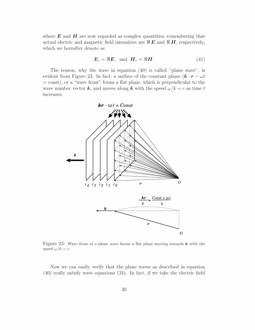
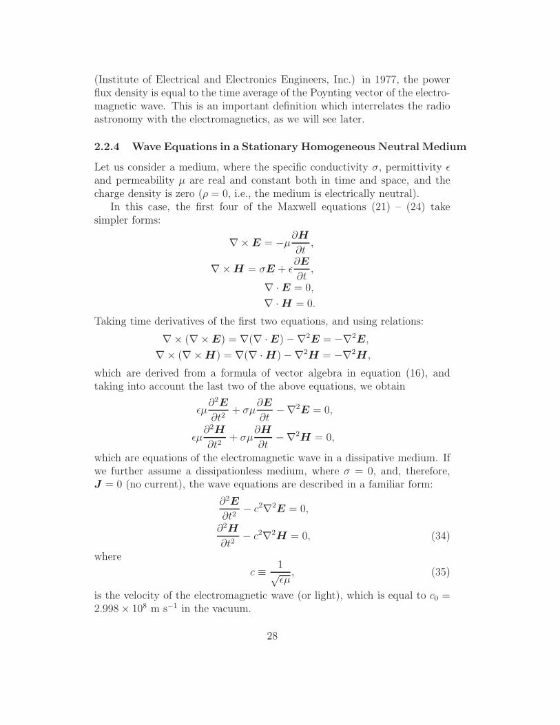
where E and H are now regarded as complex quantities, remembering thatactual electric and magnetic field intensities are ℜE and ℜH , respectively,which we hereafter denote as

Er = ℜE, and Hr = ℜH . (41)

The reason, why the wave in equation (40) is called “plane wave”, isevident from Figure 23. In fact, a surface of the constant phase (k · r − ωt= const), or a “wave front” forms a flat plane, which is perpendicular to thewave number vector k, and moves along k with the speed ω/k = c as time tincreases.

Or

r

O

k

k

t t t t3 2 1 0t 4

kr - ω t = Const

kr

k

Const + ω t

k=

Figure 23: Wave front of a plane wave forms a flat plane moving towards k with thespeed ω/k = c.

Now we can easily verify that the plane waves as described in equation(40) really satisfy wave equations (34). In fact, if we take the electric field

30

E in equation (40), for example, we have

∂2E

∂t2= E0

∂2

∂t2ei(k·r−ωt) = −ω2E0e

i(k·r−ωt) = −ω2E, (42)

and also∇2E =

∂

∂xi

∂

∂xi

E = E0∂

∂xi

∂

∂xi

ei(k·r−ωt),

where

∂

∂xi

ei(k·r−ωt) = i∂

∂xi

(k · r)ei(k·r−ωt) = i∂

∂xi

(kjxj)ei(k·r−ωt)

= ikj

∂xj

∂xi

ei(k·r−ωt) = ikjδijei(k·r−ωt) = ikie

i(k·r−ωt),

and, therefore,∂

∂xi

∂

∂xi

ei(k·r−ωt) = −k2ei(k·r−ωt),

which yields∇2E = −k2E0e

i(k·r−ωt) = −k2E. (43)

From equations (42) and (43), it is clear that the plane wave E satisfies thewave equation:

∂2E

∂t2− c2∇2E = 0,

in view of the relation ω2 = c2k2, given in equation (37), between the angularfrequency ω and the wave number k. The same discussion holds for themagnetic field H , too.

2.2.6 Electric and Magnetic Fields in a Plane Wave

Although any plane wave, with arbitrary constant E0 or H0 in equation (40),satisfies the wave equation (34), as we have just seen above, actual electricand magnetic fields in an electromagnetic wave must be mutually related toeach other, and must exhibit certain characteristic properties.

These additional properties, which will be shown below, come from thefact that the electric E and magnetic H fields must satisfy, not only the waveequations (40), where they are completely separated, but also the originalMaxwell equations, where they are related to each other.

1. The waves are transversal.In our homogeneous and neutral medium case, Maxwell equations (23)and (24) are reduced to

∇ · E = 0,

∇ · H = 0.

31

Inserting the plane wave form of the electric field E, given in equation(40), into the upper one of the above equations, we have

∇ ·E = E0i

∂

∂xi

ei(k·r−ωt) = ikiE0iei(k·r−ωt) = ik · E0e

i(k·r−ωt) = 0.

Since this relation holds for arbitrary ei(k·r−ωt), we have k ·E0 = 0 and,therefore, k · E = 0. The same argument holds for the magnetic fieldas well in the lower equation. Thus, we obtain

k · E = 0,

k · H = 0. (44)

Taking real parts of these complex equations, we easily see that theactual physical fields Er and Hr, which are the real parts Er = ℜE

and Hr = ℜH as defined in equation (41), also satisfy

k · Er = 0,

k · Hr = 0, (45)

which show that the vector fields are perpendicular to the direction n

of the wave propagation:

n ≡ k

k. (46)

This means that the plane electromagnetic waves are transversal.

2. Orthogonality of electric and magnetic fields.In our stationary, homogeneous, dissipationless (σ = 0, J = 0), andneutral (ρ = 0) medium, Maxwell equations (21) and (22) are reducedto

∇× E = −µ∂H∂t

,

∇× H = ǫ∂E

∂t.

Let us insert the plane wave forms of the electric (E) and magnetic(H) field intensities, given in equation (40), into the upper one of theabove equations.

Since(∇×E)i = ǫijkE0k

∂

∂xj

ei(k·r−ωt) = i ǫijkkjE0kei(k·r−ωt),

we obtain∇× E = ik × E.

32

Also,

∂H

∂t= H0

∂

∂tei(k·r−ωt) = −i ωH0e

i(k·r−ωt) = −i ωH .

Similar relations:

∇× H = ik × H , and∂E

∂t= −i ωE,

hold for the lower equation. Therefore, we have

k × E = µωH,

k × H = −ǫ ωE. (47)

Taking real parts of these complex equations, we obtain the same rela-tions:

k × Er = µωHr,

k × Hr = −ǫ ωEr, (48)

for the actual physical field quantities Er and Hr (equation (41)), aswell.

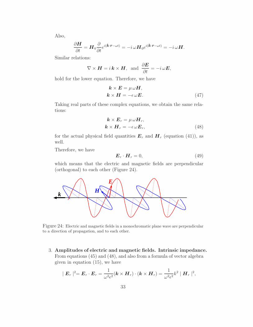
Therefore, we haveEr · Hr = 0, (49)

which means that the electric and magnetic fields are perpendicular(orthogonal) to each other (Figure 24).

E

Hk

Figure 24: Electric and magnetic fields in a monochromatic plane wave are perpendicularto a direction of propagation, and to each other.

3. Amplitudes of electric and magnetic fields. Intrinsic impedance.From equations (45) and (48), and also from a formula of vector algebragiven in equation (15), we have

| Er |2= Er · Er =1

ω2ǫ2(k × Hr) · (k × Hr) =

1

ω2ǫ2k2 | Hr |2,

33

and

| Hr |2=1

ω2µ2k2 | Er |2 .

Since we havek2

ω2=

1

c2= ǫ µ,

from equaions (37) and (35), the above two equations are equivalent,and express the same relation, describing the amplitude ratio of theelectric and magnetic fields in a monochromatic plane wave:

| Er |=√

µ

ǫ| Hr |, or | Hr |=

√

ǫ

µ| Er | . (50)

The coefficient:

Z ≡√

µ

ǫ, (51)

which is equal to

Z =| Er || Hr |

,

is called ‘intrinsic impedance’ of the medium, and is measured by aunit: [V A−1 = Ω (Ohm)], which is the same with the unit of theresistance in an electrical circuit. The value of the intrinsic impedancein the vacuum is equal to

Z0 =

√

µ0

ǫ0= 376.3 Ω.

4. Poynting vector.From equations (45) and (48), and also from equation (14) of vectoralgebra, the Poynting vetor S of the monochromatic plane wave isexpressed as

S = Er × Hr =1

ω µEr × (k × Er) =

k

ω µn | Er |2

=

√

ǫ

µn | Er |2=

1

Zn | Er |2,

where

n =k

k,

is the direction of the wave propagation as defined in equation (46),and, therefore,

S =1

Zn | Er |2= Z n | Hr |2 . (52)

34

2.3 Generation of Electromagnetic Waves

Now, let us consider generation of electromagnetic waves from a matter (froman antenna, in particular), where we must take into account existence of theelectric current and the charge.

If we try to describe this new problem, still using the electric and mag-netic field intensities E and H as basic quantities, as we did in the previoussection for the free space case, equations involved get fairly complicated. Amuch more transparent treatment is achieved, when we use so–called elec-tromagnetic potentials as basic quantities.

2.3.1 Electromagnetic Potentials

As we saw in equations (19) and (18), for any vector field F (r) and anyscalar field f(r), we have identity relations:

∇ · (∇× F ) = 0,

∇× (∇f) = 0.

It is known that following inverse relations generally hold (see, for exam-ple, “Classical Electricity and Magnetism, Second Edition” by Panofsky andPhillips, 1962):

If a relation ∇·Q(r) = 0 holds everywhere for a vector field Q(r),then such a vector field can be always expressed as a rotation ofa certain vector field F (r), i.e., Q = ∇× F .

If another relation ∇× R(r) = 0 holds everywhere for a vectorfield R(r), then such a vector field can be always expressed as agradient of a certain scalar field f(r), i.e., R = ∇f .

From Maxwell equations (24) and (21), we know that relations:

∇ · B = 0,

∇× E = −∂B∂t

,

hold everywhere.Therefore, in view of the upper one of the above two equations, we can

express the magnetic flux density B as

B = ∇× A, (53)

through an appropriate vector field A(r, t), which we call hereafter ‘vectorpotential’.

35

Then, the lower one of the above two equations now becomes

∇× (E +∂A

∂t) = 0.

Therefore, we can express the vector E + ∂A/∂t through an appropriatescalar field Φ(r, t), which we call ‘scalar potential’, as

E +∂A

∂t= −∇Φ,

and, hence, the electric field intensity E is expressed as

E = −∇Φ − ∂A

∂t. (54)

The vector potential A(r, t) and scalar potential Φ(r, t), brought to-gether, are called ‘electromagnetic potentials’. They are regarded as aux-iliary quantities, which are not directly measurable, but help to effectivelyexpress actual, physically measurable, quantities such as E and B. Units ofthe electromagnetic potentials are

A(r, t) : V s m−1,

Φ(r, t) : V,

respectively.

2.3.2 Lorentz Gauge

Electromagnetic potentials A(r, t) and Φ(r, t), which satisfy equations (53)and (54), are not unique. In fact, it is easy to confirm that for an arbitraryscalar field Λ(r, t), a new set of potentials

A′ = A + ∇Λ,

Φ′ = Φ − ∂Λ

∂t, (55)

also satisfy equations (53) and (54), if A and Φ do.It is a usual practice, in the wave generation problem, to introduce a

constraint between A and Φ called ‘Lorentz gauge’:

∇ · A + ǫ µ∂Φ

∂t= 0, (56)

36

using the above ambiguity, or, better to say, the freedom. The Lorentzgauge, as given in equation (56), allows us to formulate the generation ofelectromagnetic waves in a very smart way, as we will see below.

It is remarkable that any electromagnetic potentials An and Φn, whichoriginally do not satisfy the Lorentz gauge:

∇ · An + ǫ µ∂Φn

∂t6= 0,

can be converted to new ones Ay and Φy fulfilling the Lorentz gauge equation(56), by using a scalar field Λ in equation (55):

Ay = An + ∇Λ, and Φy = Φn − ∂Λ

∂t,

which satisfies an equation:

ǫ µ∂2Λ

∂t2−∇2Λ = ∇ · An + ǫ µ

∂Φn

∂t.

Of course, the physically measurable fields, such as E and B, are not affectedby this conversion.

Therefore, we can always select electromagnetic potentials A and Φ,which correspond to real electromagnetic fields through equations (53) and(54), and, at the same time, satisfy the Lorentz gauge (equation (56)):

B = ∇× A,

E = −∇Φ − ∂A

∂t,

∇ · A + ǫ µ∂Φ

∂t= 0.

Hereafter, we will consider only such electromagnetic potentials.

2.3.3 Wave Equations with Source Terms

We will assume, for simplicity, a homogeneous and stationary medium withrespect to the permittivity ǫ and the permeability µ, i.e., ǫ = const and µ =const both in time and space.

Inserting equations (53) and (54) into a Maxwell equation (22):

∇× H = J + ǫ∂E

∂t,

we have1

µ∇× (∇× A) = J − ǫ (

∂2A

∂t2+ ∇∂Φ

∂t).

37

In view of equation (16), this equation is reduced to

∇(∇ · A) −∇2A = µJ − ǫ µ∂2A

∂t2− ǫ µ∇∂Φ

∂t,

and, then,

∇2A − ǫ µ∂2A

∂t2= −µJ + ∇(∇ · A + ǫ µ

∂Φ

∂t) = −µJ ,

where we used equation (56) of the Lorentz gauge.Also, another Maxwell equation (23):

ǫ∇ · E = ρ,

can be expressed as

−ǫ∇ · (∇Φ +∂A

∂t) = ρ,

through the electromagnetic potentials, and is reduced to

∇2Φ +∂

∂t(∇ · A) = −1

ǫρ,

and, then

∇2Φ − ǫ µ∂2Φ

∂t2= −1

ǫρ,

where we again used equation (56) of the Lorentz gauge.Introducing again the light velocity c (c2 = 1 / ǫ µ), we obtain equations

∇2A − 1

c2∂2A

∂t2= −µJ , (57)

∇2Φ − 1

c2∂2Φ

∂t2= −1

ǫρ, (58)

which have the simple form of the wave equation. The only difference fromthe free space case in equation (34) is the existence of RHS terms, which aresource terms of the wave equations. These equations describe the interactionof the electric current J and charge ρ within a source region with the electro-magnetic waves A and Φ, i.e., the current and charge may generate the wavesin a free space (transmission), or the waves in the free space may generate thecurrent and charge in the source region (reception), as schematically shownin Figure 25.

Equations (57) and (58) are consistent with equation (56) of the Lorentzgauge, as we can easily verify using equation (29) of continuity (or conserva-tion) of electric charge.

38

J, ρ

source region

A, φ

reception

transmission

Figure 25: A schematic view of the interaction of the current and charge in a sourceregion with the electromagnetic waves in a free space.

2.3.4 Solution of the Wave Equation with the Source Term

Let us consider solutions of equations (57) and (58). Since each componentof vector equation (57) and scalar equation (58) have the same general formof

∇2Ψ(r, t) − 1

c2∂2Ψ(r, t)

∂t2= −f(r, t), (59)

where f and Ψ are functions of the time t and the space r, we will confineourselves to seeking a solution Ψ(r, t) of equation (59) with a source term−f(r, t). We assume that the source term takes some finite value only withina certain source region.

In order to express the RHS of equation (59) in an integral form, we useDirac’s delta function δ(r), which has following functional properties:

δ(r) = 0, when r 6= 0,∫

V

δ(r − r′) dV ′ = 1,

∫

V

F (r′)δ(r − r′) dV ′ = F (r), for any function F (r),

where r′ is a variable radius vector with elements x′1, x′2, and x′3, dV

′ =dx′1dx

′2dx

′3 is a volume element, and the integration is taken over some volume

V containing a point r. Now we can express the RHS of equation (59) as:

∇2Ψ(r, t) − 1

c2∂2Ψ(r, t)

∂t2= −

∫

V

f(r′, t)δ(r − r′) dV ′, (60)

39

dV’ r’

r-r’

r

O

source medium

f(r)=0

r*

V

with /f(r)=0

Figure 26: Geometry of the source medium region.

where the integration is taken over an appropriate volume V , containing thesource region and a point r (see Figure 26).

Using this form, we will solve the equation in terms of the Green func-tion method, which works in the following way.

• Consider the wave equation with a time-variable point source at theorigin O with r = 0:

∇2ψ − 1

c2∂2ψ

∂t2= −f(r∗, t)δ(r), (61)

where r∗ denotes some particular point in the source region, and−f(r∗, t)is a function of time t.

• If ψ(r∗, r, t) is a solution of the above equation (which is the Greenfunction), then, ψ(r∗, r − r′, t) must be a solution of equation:

∇2ψ − 1

c2∂2ψ

∂t2= −f(r∗, t)δ(r − r′),

for any r′.

• Therefore, ψ(r′, r − r′, t) must be a solution of equation:

∇2ψ − 1

c2∂2ψ

∂t2= −f(r′, t)δ(r − r′),

in a special case when r∗ = r′.

• Finally, in view of the principle of superposition of solutions in a linearequation, an integral of the function ψ(r′, r − r′, t) with respect to r′:

Ψ(r, t) =

∫

V

ψ(r′, r − r′, t) dV ′, (62)

40

must be a solution of our wave equation (60):

∇2Ψ(r, t) − 1

c2∂2Ψ(r, t)

∂t2= −

∫

V

f(r′, t)δ(r − r′) dV ′.

Thus, the solution ψ(r∗, r, t) of equation (61) is really a Green function,which enables us to obtain a solution of equation (60), or equivalently equa-tion (59).

Now, we can express the solution ψ(r∗, r, t) (Green function) in a form:

ψ(r∗, r, t) =f(r∗, t ∓ r

c)

4πr, (63)

where r is the length of the radius vector r, i.e. r =| r |= √xixi =

√

x21 + x2

2 + x23. Let us veryfy this in the following way.

1. We use following general formulae.

• For a radius vector r,

∇r =r

r, and ∇ · r = 3, since (64)

(∇r)i =∂r

∂xi

=∂

∂xi

√xjxj =

1

2√xjxj

∂

∂xi

(xkxk) =xi

r,

and ∇ · r =∂xi

∂xi

= δii = 3.

• For a function R(r) of the radius r,

∇2R(r) =d2R(r)

dr2+

2

r

dR(r)

dr, since (65)

∇2R(r) = ∇ · ∇R(r) = ∇ ·(

dR

dr∇r

)

= ∇ ·(

dR

dr

r

r

)

= ∇(

1

r

dR

dr

)

· r +

(

1

r

dR

dr

)

∇ · r

= rd

dr

(

1

r

dR

dr

)

+ 3

(

1

r

dR

dr

)

=d2R

dr2+

2

r

dR

dr.

• For a particular function 1/r, which is singular at the origin, we have

∇2

(

1

r

)

= −4π δ(r), (66)

41

as we know from the potential theory (electrostatic potential arounda point charge, Newtonian gravitaional potential around a point mass,etc., ...). We can veryfy this equation by integrating both sides throughan arbitrary volume V , covered by a surface S with a normal n, andapply to the LHS Gauss’s integration theorem:

∫

V

∇ · A dV =

∮

S

A · n dS, (67)

where A is an arbitrary vector field, V is a closed volume, covered bya surface S with a normal vector n.

In fact, the RHS gives

−4π

∫

V

δ(r) dV =

−4π (if V contains the origin r = 0),

0 (otherwise),

and the LHS also yields

∫

V

∇·∇(

1

r

)

dV =

∮

S

∇(

1

r

)

·n dS = −∮

S

r

r3·n dS =

−∮

dΩ = −4π,

0,

depending again if V contains the origin or not, where dΩ is a solidangle element.

2. Let us introduce a notation:

u ≡ t∓ r

c.

Then, the function ψ in equation (63) is now expressed as

ψ(r∗, r, t) =f(r∗, u)

4πr.

Noting that

∂f

∂t=df

du

∂u

∂t,

∂f

∂r=df

du

∂u

∂r, with

∂u

∂t= 1, and

∂u

∂r= ∓1

c,

we obtain∂2ψ

∂t2=

1

4πr

d2f

du2,

42

and, using equation (65),

∇2ψ =1

4πr∇2f + 2∇

(

1

4πr

)

· ∇f + f ∇2

(

1

4πr

)

=1

4πr

(

∂2f

∂r2+

2

r

∂f

∂r

)

− 2

4πr2

∂f

∂r− f δ(r)

=1

4πr

1

c2d2f

du2− f δ(r).

Therefore, the function ψ(r∗, r, t) in equation (63) really satisfies the waveequation (61) with a point source term at the origin:

∇2ψ − 1

c2∂2ψ

∂t2= −f(r∗, u) δ(r) = −f(r∗, t∓

r

c) δ(r) = −f(r∗, t) δ(r),

and, hence, can be used as a Green function for solving equation (59) in theform given in equation (62).

2.3.5 Retarded Potential

Now, from equations (62) and (63), a solution of the wave equation with thesource term (59) is expressed as:

Ψ(r, t) =1

4π

∫

V

f(r′, t∓ |r−r′|c

)

| r − r′ | dV ′. (68)

In actuality, there are two choices of solutions corresponding to ‘+’ signand ‘−’ sign of the ∓ term in the numerator of the integrand. One solutionwith ‘−’ sign is called ‘retarded potential’, and another with ‘+’ sign is called‘advanced potential’.

Meanings of the retarded and advanced potentials can be better under-stood in the simplest case of the point source term at the origin (r = 0),when the solution takes the same form as the one in equation (63):

Ψ(r, t) =g(t ∓ r

c)

4πr,

where g(t) is a function describing the time variation of the source term.First we consider the retarded potential case with ‘−’ sign. In this case,

the function g(t − rc) keeps a constant value as far as the argument t − r

cis

constant. This means that the retarded potential

Ψ(r, t) =g(t − r

c)

4πr,

43

t

r

retardedpotential

advancedpotential

sourceregion

Figure 27: Pattern propagations in retarded and advanced potentials.

describes some pattern of time variation (for example, a sinusoidal oscilla-tion), originated in the source region (a point in this case), propagatingoutward with velocity c, and decreasing its amplitude in proportion to 1/r.The pattern at a distant point (with larger r) is retarded compared withthe one at a near point (with smaller r). This shows a typical example ofthe transmission of the electromagnetic wave from the source region (Figure27).

On the other hand, the advanced potential with ‘+’ sign describes thatsome pattern of time variation propagates inward, and induces the samesort of time variation in the source region. The pattern at a distant point(with larger r) is advanced compared with the one at a near point (withsmaller r). This obviously represents the reception of the electromagneticwave, coming from outside, at the source region (Figure 27). However, thisis not a ‘typical’ example of the wave reception, because the proportionalityto 1/r implies that the incoming wave must be amplified as it approaches tothe source region. This occurs, for example, in the converging wave reflectedby a paraboloidal mirror of a radio telescope antenna, but in a limited space–time range.

We will consider, hereafter, the problem of the transmission of electro-magnetic waves from a source region (or an antenna). Therefore, we will usethe retarded potential only.

Coming back to the electromagnetics, we obtain retarded potential solu-

44

tions for wave equations (57) and (58) with source terms as follows:

A(r, t) =µ

4π

∫

J(r′, t− |r−r′|c

)

| r − r′ | dV ′, (69)

Φ(r, t) =1

4πǫ

∫

ρ(r′, t− |r−r′|c

)

| r − r′ | dV ′. (70)

Since the vector potential A and the scalar potential Φ derived here are notindependent to each other, but related by Lorentz gauge in equation (56):

∇A + ǫµ∂Φ

∂t= 0,

we will consider hereafter the vector potential A only.

2.3.6 Transmission of Radio Wave from a Harmonically Oscillat-ing Source

Let us consider a case when the current density J(r, t) is harmonically (or,sinusoidally) oscillating everywhere in a source region with the same angularfrequency ω = 2πν:

J(r, t) = J(r)e−iωt. (71)

In this complex representation, we again use the convention, that the actualphysical quantity is expressed by the real part of the complex quantity (in theabove particular example, the actual current density is ℜ [J(r)e−iωt]). Theassumption of the same frequency throughout the source region, and theresultant separation of spatial and temporal variables, might seem a littleartificial. But this must be valid for a frequency component in a Fourierexpansion of the time variable current density.

The vector potential A(r, t), generated by such a current, is also ex-pressed in a similar form:

A(r, t) = A(r)e−iωt. (72)

In fact, inserting equation (71) to the formula of the retarded potential inequation (69), we obtain

A(r, t) =µ

4π

∫

J(r′, t− |r−r′|c

)

| r − r′ | dV ′ =

[

µ

4π

∫

J(r′)eik|r−r′|

| r − r′ | dV′]

e−iωt,

where k ≡ ω/c = 2π/λ, with λ being the wavelength corresponding to theangular frequency ω. Therefore, we know that A(r, t) is really expressed in

45

the form of equation (72), with

A(r) =µ

4π

∫

J(r′)eik|r−r′|

| r − r′ | dV′. (73)

Since harmonically oscillating current density J(r, t) = J(r) e−iωt gen-erates oscillating vector potential A(r, t) = A(r) e−iωt, it also generatesoscillating electric and magnetic field intensities as well, according to equa-tions:

B = ∇× A, and ∇× H = J +∂D

∂t,

which are the definition of the vector potential and one of the Maxwell equa-tions. In homogeneous medium outside of the source region, where we haveno current (J = 0) and ǫ, µ = const, the above equations are reduced to

H =1

µ∇× A, (74)

and−iωǫE = ∇× H . (75)

Therefore, the generated magnetic and electric fields are expressed as:

H(r, t) = H(r)e−iωt, with H(r) =1

µ∇× A(r), (76)

E(r, t) = E(r)e−iωt, with E(r) = ic

k∇× (∇× A(r)), (77)

where we used the relations c2 = 1/ǫµ and ω = kc.

2.3.7 Electromagnetic Fields Far from the Source Region

Let us now calculate the electromagnetic fields generated by the harmoni-cally oscillating current in the source region, taking into account the explicitexpression for A(r), given in equation (73). For definiteness, we choose theorigin of radius vectors r and r′ within the source region. Note that r rep-resents an arbitrary point in space, but r′ is meaningful within the sourceregion only, in equation (73).

i–th component of the rotation of A(r) in equation (76) is given by

(∇× A(r))i = ǫijk∂

∂xjAk(r) =

µ

4πǫijk

∫

Jk(r′)∂

∂xj

eik|r−r′|

| r − r′ | dV′. (78)

Since∂

∂xi| r − r′ |= xi − x′i

| r − r′ | ,

46

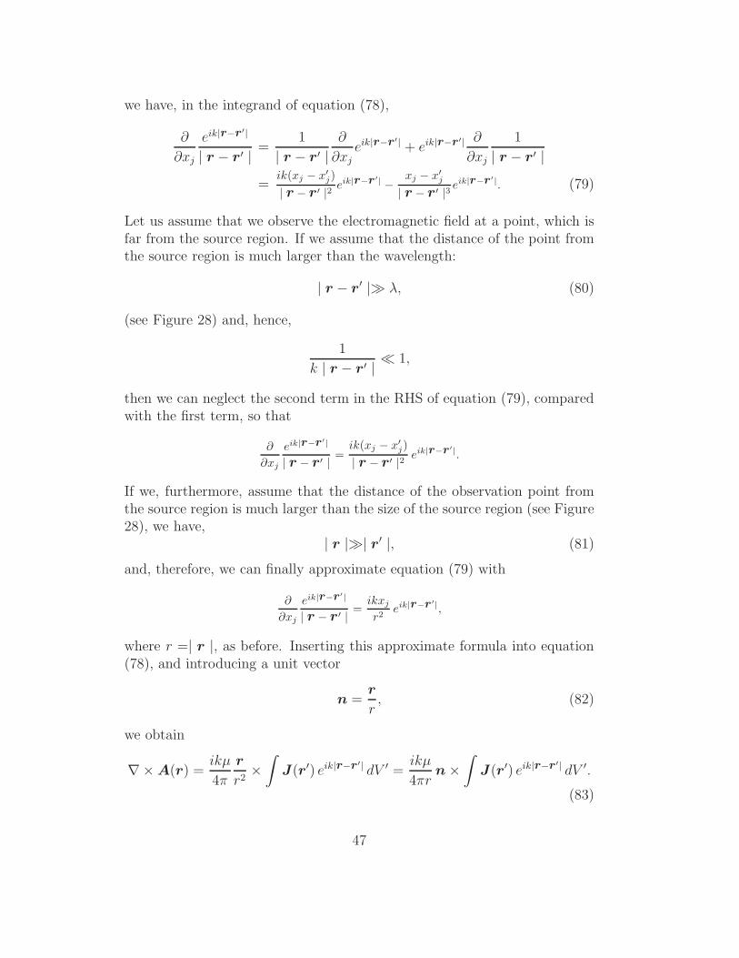
we have, in the integrand of equation (78),

∂

∂xj

eik|r−r′|

| r − r′ | =1

| r − r′ |∂

∂xj

eik|r−r′| + eik|r−r′| ∂

∂xj

1

| r − r′ |

=ik(xj − x′

j)

| r − r′ |2 eik|r−r′| −xj − x′

j

| r − r′ |3 eik|r−r′|. (79)

Let us assume that we observe the electromagnetic field at a point, which isfar from the source region. If we assume that the distance of the point fromthe source region is much larger than the wavelength:

| r − r′ |≫ λ, (80)

(see Figure 28) and, hence,

1

k | r − r′ | ≪ 1,

then we can neglect the second term in the RHS of equation (79), comparedwith the first term, so that

∂

∂xj

eik|r−r′|

| r − r′ | =ik(xj − x′

j)

| r − r′ |2 eik|r−r′|.

If we, furthermore, assume that the distance of the observation point fromthe source region is much larger than the size of the source region (see Figure28), we have,

| r |≫| r′ |, (81)

and, therefore, we can finally approximate equation (79) with

∂

∂xj

eik|r−r′|

| r − r′ | =ikxj

r2eik|r−r′|,

where r =| r |, as before. Inserting this approximate formula into equation(78), and introducing a unit vector

n =r

r, (82)

we obtain

∇× A(r) =ikµ

4π

r

r2×

∫

J(r′) eik|r−r′| dV ′ =ikµ

4πrn ×

∫

J(r′) eik|r−r′| dV ′.

(83)

47

The same sort of discussions, under the same approximations of equations(80) and (81), lead to

∇× (∇× A(r)) = −k2µ

4πrn × (n ×

∫

J(r′) eik|r−r′| dV ′). (84)

Therefore, in view of equations (73), (76) and (77), we have approximateformulae for the vector potential, magnetic field and electric field:

A(r) =µ

4πr

∫

J (r′) eik|r−r′| dV ′, (85)

H(r) =1

µ∇×A(r) =

ik

4πrn ×

∫

J (r′) eik|r−r′| dV ′, (86)

E(r) =c

k∇× (∇×A(r)) = − iZk

4πrn × (n ×

∫

J(r′) eik|r−r′| dV ′), (87)

where Z =√

µ/ǫ is the intrinsic impedance, as defined in equation (51), andwe used relation c = 1/

√ǫµ, as given in equation (35).

2.3.8 Far Field Solution and Fraunhofer Region

It is worth to note that we did not approximate | r−r′ | by r in the argumentsof exponential functions in equations (85), (86) and (87), even though weassumed that | r |≫| r′ |. Such approximation is not valid, in general, inan argument (or phase) of any sinusoidal function, since only remainder ofthe argument divided by 2π is meaningful in such a function (for example,cos(983517826 + 132) = cos(983517826 × (1 + 1.34212107 × 10−7)) is notclose to cos(983517826) at all).

However, if we find an ‘absolutely’ small term in the argument, which ismuch smaller than 1 radian, say, we can safely neglect such a term, and thismay allow us to derive a useful approximate formula.

Let a characteristic size of our source region (aperture diameter of anantenna, for example) be D, distance to the observation point from the originin the source region be r, and the wavelength be λ = 2π/k. We can generallyexpand the argument in the exponential term k | r−r′ | into a Taylor series:

k | r − r′ |= k√

r2 − 2r · r′ + r′2 ∼= kr (1 − r · r′

r2+

1

2

r′2

r2+ · · · ). (88)

If a condition, which is called “Fraunhofer condition”,

2D2

λ≪ r, (89)

is satisfied among r, D and λ (see Figure 28), the third term in the expansion

48

O

r

D

Source region

Observation point

l

J

r’

r ~ D

|r-r’|~ λ

Fresnel Region

Fraunhofer region

J = 0

µ, ε = const r ~ 2D / λ2

Figure 28: Fraunhofer condition.

of equation (88) fulfills

1

2kr′2

r∼ π

λ

D2

r≪ π

2≈ 1.57 radian.

Therefore, we can neglect the third and higher order terms in the expansionof equation (88), in the argument of the exponential function, and obtain

eik|r−r′| ∼= eikr−ikn·r′

, (90)

where n = r/r, as before. Note that, on the contrary, the second term hasthe order of magnitude of

kn · r′ ∼ 2πD

λ,

and cannot be neglected at all, in general, in the argument of the exponential(or, sinusoidal) function.

In this approximation, equation (85) for the vector potential, in particu-lar, is expressed as

A(r) =µ

4π

eikr

r

∫

J (r′) e−ikn·r′

dV ′.

Now the integral term is a function of the direction n only, and does notdepend on the distance r to the observation point.

49

The region where r > 2D2/λ is called “Fraunhofer region” or “farfield”, and the region where r < 2D2/λ is called “Fresnel region” or“near field”.

In the Fraunhofer region, we can approximate the exponential term asshown in equation (90). Therefore, introducing a vector T (n), characterizinga directional pattern of the radiation in the far field,

T (n) =

∫

J(r′)e−ikn·r′

dV ′, (91)

and taking into account the temporal variation of the electromagnetic fields,we obtain, from equations (72), (76), (77), (85), (86), (87) and (90), so–calledfar field solutions:

A(r, t) =µ

4π

ei(kr−ωt)

rT (n), (92)

H(r, t) = i1

2λ

ei(kr−ωt)

rn × T (n), (93)

E(r, t) = −i Z2λ

ei(kr−ωt)

rn × [n × T (n)]. (94)

These equations describe harmonically oscillating and spherically expandingdirectional patterns T (n), n×T (n), and n× [n×T (n)], i.e. the sphericalwaves.

It is clear from equations (93) and (94), that we have

n · H = 0, n · E = 0, and H · E = 0, (95)

which imply that the magnetic H and electronic E waves are transversaland mutually orthogonal. It is also clear from the same equations that

E = −Z n × H , and H =1

Zn × E. (96)

Taking real parts of these complex equations, we see that the same relationshold for actual electromagnetic fields, which are real parts of the complexexpressions: Hr = ℜH and Er = ℜE, i.e.

Er = −Z n × Hr, and Hr =1

Zn × Er.

Therefore, the Poynting vector S for the spherical wave is expressed as:

S = Er × Hr = Z n | Hr |2=1

Zn | Er |2 . (97)

50

This equation means that the Poynting vector of the spherical wave is di-rected towards n = r/r, which is nothing but the direction of propagationof the wave, and the amplitude ratio of the electric and magnetic fields is

| Er || Hr |

= Z, (98)

i.e. equal to the intrinsic impedance of the medium Z =√

µ/ǫ. Theseproperties are the same with those in the plane wave case, which we discussedearlier. Of course, the spherical waves locally approach to the plane waveswhen r → ∞.

2.3.9 Hertz Dipole

i2

i3

i1

θ

φ

l

q

r

Figure 29: Hertz dipole.

We are now in position to derive some results on transmission of theelectromagnetic waves from simple antennas, using the far field solutions inequations (92), (93) and (94). First, we will consider an idealized antenna,composed of an infinitesimal electric dipole called “Hertz dipole”, which wasdiscussed by Heinrich Hertz in 1888.

Let us consider an infinitesimally small cylinder with infinitesimal crosssection q and infinitesimal length l, which is located at the origin of a rect-angular coordinate system and directed towards 3–rd axis (Figure 29).

Let us assume a homogeneous electric current I, which is flowing withinthe cylinder and harmonically oscillating in time proportionally to e−iωt.

In this case, the vector T (n) characterizing the radiation pattern in thefar field in equation (91) takes a particularly simple form. In fact, if weassume that l ≪ λ, where λ is the wavelength, we have

kn · r′ ∼ 2π

λl ≪ 1, and, therefore, e−ikn·r′ ∼= 1,

51

in equation (91), and, consequently,

T (n) =

∫

J dV ′ = J l q = I l i3, (99)

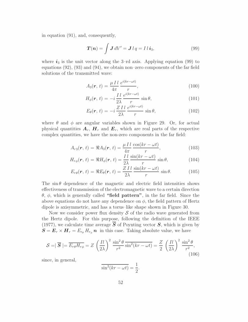
where i3 is the unit vector along the 3–rd axis. Applying equation (99) toequations (92), (93) and (94), we obtain non–zero components of the far fieldsolutions of the transmitted wave:

A3(r, t) =µ I l

4π

ei(kr−ωt)

r, (100)

Hφ(r, t) = −i I l2λ

ei(kr−ωt)

rsin θ, (101)

Eθ(r, t) = −i Z I l2λ

ei(kr−ωt)

rsin θ, (102)

where θ and φ are angular variables shown in Figure 29. Or, for actualphysical quantities Ar, Hr and Er, which are real parts of the respectivecomplex quantities, we have the non-zero components in the far field:

Ar3(r, t) = ℜA3(r, t) =µ I l

4π

cos(kr − ωt)

r, (103)

Hrφ(r, t) = ℜHφ(r, t) =I l

2λ

sin(kr − ωt)

rsin θ, (104)

Erθ(r, t) = ℜEθ(r, t) =Z I l

2λ

sin(kr − ωt)

rsin θ. (105)

The sin θ dependence of the magnetic and electric field intensities showseffectiveness of transmission of the electromagnetic wave to a certain directionθ, φ, which is generally called “field pattern”, in the far field. Since theabove equations do not have any dependence on φ, the field pattern of Hertzdipole is axisymmetric, and has a torus–like shape shown in Figure 30.

Now we consider power flux density S of the radio wave generated fromthe Hertz dipole. For this purpose, following the definition of the IEEE(1977), we calculate time average S of Poynting vector S, which is given byS = Er × Hr = Erθ

Hrφn in this case. Taking absolute value, we have

S =| S |= ErθHrφ = Z

(

Il

2λ

)2sin2 θ

r2sin2(kr − ωt) =

Z

2

(

Il

2λ

)2sin2 θ

r2,

(106)since, in general,

sin2(kr − ωt) =1

2.

52

θ

Figure 30: Field pattern of Hertz dipole.

θ

Figure 31: Power pattern of Hertz dipole.

The sin2 θ dependence shows effectiveness of transmission of the power ofthe electromagnetic wave to a certain direction, which is called the “powerpattern” (Figure 31).

Figure 32 shows time variation of the electromagnetic field in the nearfield of the oscillating Hertz dipole, which can be calculated using exactequations (73), (76) and (77).This figure is copied from a webpage

http://didaktik.physik.uni-wuerzburg.de/∼pkrahmer/home/dipol.html.One can see an animation movie of the transmission of the electromagneticwave from the Hertz dipole in this webpage.

2.3.10 Linear Dipole Antenna of Finite Length

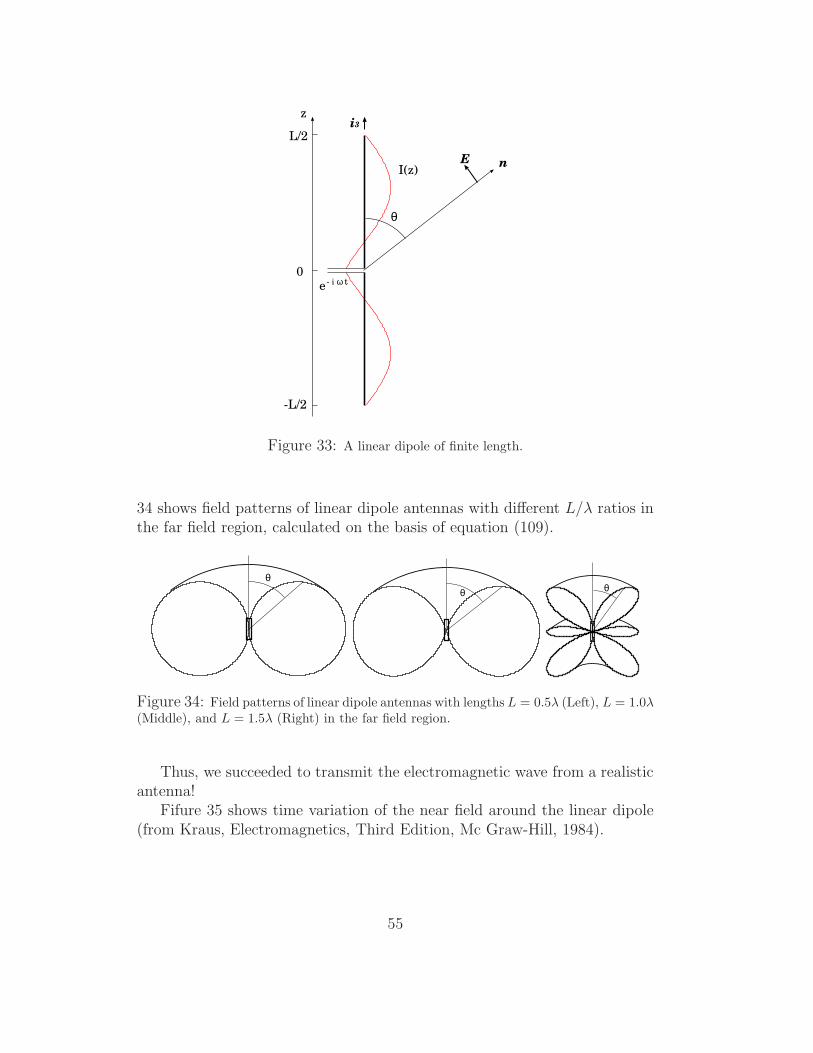
The Hertz dipole was still an idealized antenna. We now consider a realisticantenna, a linear dipole of finite length, with an oscillating current fed fromits center (Figure 33).

Let us assume that a linear dipole of length L is directed towards i3 axisand its center is located at the origin. Let us also assume that the spatialdistribution of the harmonically oscillating electric current (∝ exp(−iωt)) is

53

Figure 32: Time variation of the electromagnetic field close to the Hertz dipole (fromhttp://didaktik.physik.uni-wuerzburg.de/∼pkrahmer/home/dipol.html).

given by an empirical formula:

I(z) = I0 sin

[

k

(

L

2− | z |

)]

, (107)

where z is distance from the origin along i3 axis, and k = 2π/λ.Then, in the far field, we have

T (n) =

∫

J(r′)e−ikn·r′

dV ′ = i3

∫ L/2

−L/2

I(z)e−ikz cos θ dz

= I0 i3

∫ L/2

−L/2

sin

[

k

(

L

2− | z |

)]

e−ikz cos θ dz

= 2 I0 i3

∫ L/2

0

sin

(

kL

2− kz

)

cos(kz cos θ) dz

=2 I0

k sin2 θi3

[

cos

(

kL

2cos θ

)

− cos

(

kL

2

)]

, (108)

where θ is an angle of the direction of propagation n from the i3 axis. There-fore, equation (94) gives a non–zero component of the far field solution ofthe electric field:

Eθ(r, t) = −i ZI02π

ei(kr−ωt)

r

cos(

kL2

cos θ)

− cos(

kL2

)

sin θ. (109)

This result shows that the field pattern of the linear dipole antenna is differentwith different ratio L/λ between the dipole length and wavelength. Figure

54

θ

I(z)n

i3

L/2

-L/2

E

- i ω te0

z

Figure 33: A linear dipole of finite length.

34 shows field patterns of linear dipole antennas with different L/λ ratios inthe far field region, calculated on the basis of equation (109).

θθ θ

Figure 34: Field patterns of linear dipole antennas with lengths L = 0.5λ (Left), L = 1.0λ(Middle), and L = 1.5λ (Right) in the far field region.

Thus, we succeeded to transmit the electromagnetic wave from a realisticantenna!

Fifure 35 shows time variation of the near field around the linear dipole(from Kraus, Electromagnetics, Third Edition, Mc Graw-Hill, 1984).

55

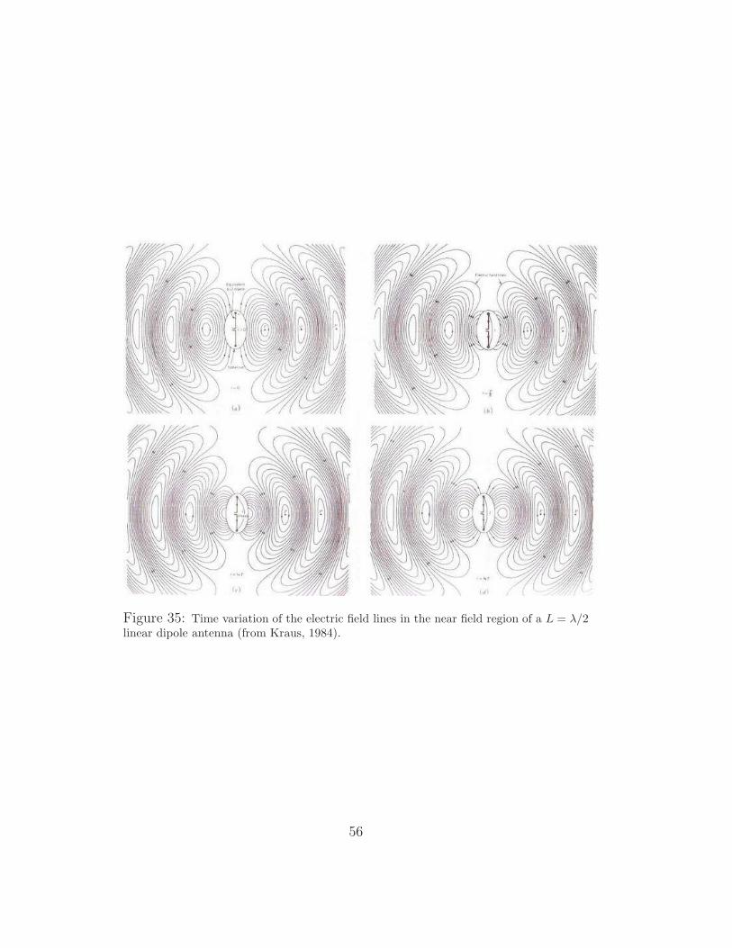
Figure 35: Time variation of the electric field lines in the near field region of a L = λ/2linear dipole antenna (from Kraus, 1984).

56

2.4 Transmitting and Receiving Antennas

2.4.1 The Reciprocity Theorem

We derived field patterns of the simplest dipole antennas as dependences oftransmitted electromagnetic fields on different directions, which characterizetransmission efficiencies towards those directions. It is well known that thesame antennas can be used both for transmission and reception of the elec-tromagnetic waves. For receptions, we also call “field patterns” or “voltagereception patterns” the efficiencies of the reception from an emitter at dif-ferent directions. Then, how the transmission and reception field patternsof the same antenna are related to each other? In order to answer to thisquestion, we will consider Rayleigh’s Reciprocity Theorem (1894) as appliedto the electromagetics.

The reciprocity theorem states the followings.

Let the electromagnetic fields, generated by two source currentsJ1 and J2, be E1, H1 and E2, H2, respectively. If the sourcecurrents exist within two finite spatial regions V1 and V2 only(Figure 36), and if a volume V includes both the two regions,then we have

∫

V

(E1 · J2 − E2 · J1) dV = 0. (110)

Let us prove this theorem in a case of homogeneous medium (ǫ, µ =const), and harmonically oscillating currents (∝ exp(−iωt)). In this case,from Maxwell equations (21) and (22), we have:

∇× H1 = J1 − iωǫE1, ∇× H2 = J2 − iωǫE2, (111)

∇× E1 = iωµH1, ∇× E2 = iωµH2. (112)

Using a formula of vector algebra in equation (17):

∇ · (A × B) = B · (∇× A) − A · (∇× B),

and equations (111) and (112), we have

∇ · (E1 × H2) = H2 · (∇× E1) − E1 · (∇× H2)

= iωµH1 · H2 − E1 · J2 + iωǫE1 · E2,

∇ · (E2 × H1) = H1 · (∇× E2) − E2 · (∇× H1)

= iωµH1 · H2 − E2 · J1 + iωǫE1 · E2.

57

J1

J2

E1, H1

E2, H2

V2

V1

Figure 36: Electromagnetic fields generated by two source currents confined within twofinite spatial regions.

Taking difference of the above equations, we obtain

∇ · (E1 × H2 − E2 × H1) = E2 · J1 − E1 · J2.

Then, integrating the both sides of the above equation through the volumeV , which includes source regions of both J1 and J2, and applying Gauss’sintegration theorem in equation (67) to the LHS, we have

∮

(E1 × H2 − E2 × H1) · nndS =

∫

V

(E2 · J1 − E1 · J2) dV, (113)

where nndS is a vector of the surface element on the volume V with a unitnormal vector nn.

Let us denote radius vectors from centers of the two source current regionsto a point on the surface (point A, say) of the volume V as r1 and r2, andlet us also denote a radius vector from the origin O, at the Middle point ofthe two current regions, to the point A as r, as shown in Figure 37.

If we adopt a sufficiently big volume V , so that its surface is in far fieldregions from the two current regions, the electromagnetic fields are approxi-mated by the spherical waves, which satisfy

E1 = −Z n1 × H1, E2 = −Z n2 × H2, (114)

58

O

dS

r1 r r2

n2 n n1

J1 J2

A

Figure 37: Geometry of the source current regions and radius vectors to a point on thesurface of the volume V .

where n1 = r1/r1 and n2 = r2/r2.Let us further assume, for simplicity, that the surface is a sphere with the

center at the origin O. In that case, the unit normal vector nn to the surfaceelement at the point A is nn = n = r/r. Then, the surface integral in theLHS of equation (113) becomes

∮

(E1 × H2 − E2 × H1) · nn dS

= − Z

∮

[(n1 × H1) × H2 − (n2 × H2) × H1] · n dS

= − Z

∮

[(n · H1)(n1 · H2) − (n · H2)(n2 · H1)

− n · (n1 − n2)(H1 · H2)] dS

= − Z

∮

[(n · H1)(n1 − n) · H2 − (n · H2)(n2 − n) · H1

− n · (n1 − n2)(H1 · H2)] dS, (115)

where we used a formula of vector algebra

A × (B × C) = B(A · C) − C(A · B),

given in equation (14).Now, if we tend the radius r of the sphere to the infinity (r → ∞), then

59

dS ∝ r2, since dS = r2 sin θ dθ dφ,

| H1 | | H2 |∝ r−2, because they are spherical waves,

n1 → n, n2 → n, hence n1 − n → 0, n2 − n → 0, n1 − n2 → 0.

Consequently, the LHS of equation (115), and therefore LHS of equation(113), too, tends to zero, when r → ∞.

Thus, for a sufficiently large spherical volume V , equation (113) gives us∫

V

(E2 · J1 − E1 · J2)dV = 0. (116)

But, since we assume that the currents J1 = 0 and J2 = 0 outside ofthe finite regions V1 and V2, respectively, equation (116) must hold for anarbitrary volume V , including V1 and V2. Thus, we proved the reciprocitytheorem.

Equation (116) can be expressed also in a form:∫

V1

E2 · J1 dV =

∫

V2

E1 · J2 dV. (117)

2.4.2 Equivalence of Field Patterns in Transmission and Recep-tion

Figure 38: Transmission (Left) and reception (Right) field patterns of an antenna.

Suppose an antenna, which is transmitting the radio wave towards the sky.The transmission field pattern is defined as the direction dependence

60

of the amplitude of the electromagnetic field transmitted from the antenna(see left panel of Figure 38). Now suppose the same antenna is receivingradio wave from a hypothetical distant emitter of unit strength located inan arbitrary direction of the sky. The reception field pattern, or voltagereception pattern, is defined as dependence of the amplitude of the receivedelectromagnetic field, or the resultant voltage in a receiver system, on thedirection of the emitter (see right panel of Figure 38).

The reciprocity theorem shows us that the transmission field pattern andthe reception field pattern of the same antenna are identical.

In order to prove this statement, let us again consider that a current J1

in an antenna 1 generates an electric field E1 around another antenna 2,while a current J2 in the antenna 2 generates an electric field E2 around theantenna 1 (see Figure 36).

Let us assume, for simplicity, that the antennas are small dipoles withlength l and cross–section q (Figure 39). This is not necessarily a very un-

l

q

dV

Figure 39: A small dipole with length l and cross-section q.

realistic assumption, since co–axial to waveguide converters in feedhorns ofexisting antennas are often composed of simple dipoles. Then, we can adoptin equation (117),

volume element : dV = ql

current : I =| J | qvoltage : U = El.

And, therefore, equation (117) can now be expressed as:

U2 I1 = U1 I2. (118)

Let us now consider that antenna 1 is fixed at some position and antenna 2moves from position A to position B, and then to position C (Figure 40).Let us denote voltages, generated by the current I1 in antenna 1 at positions

61

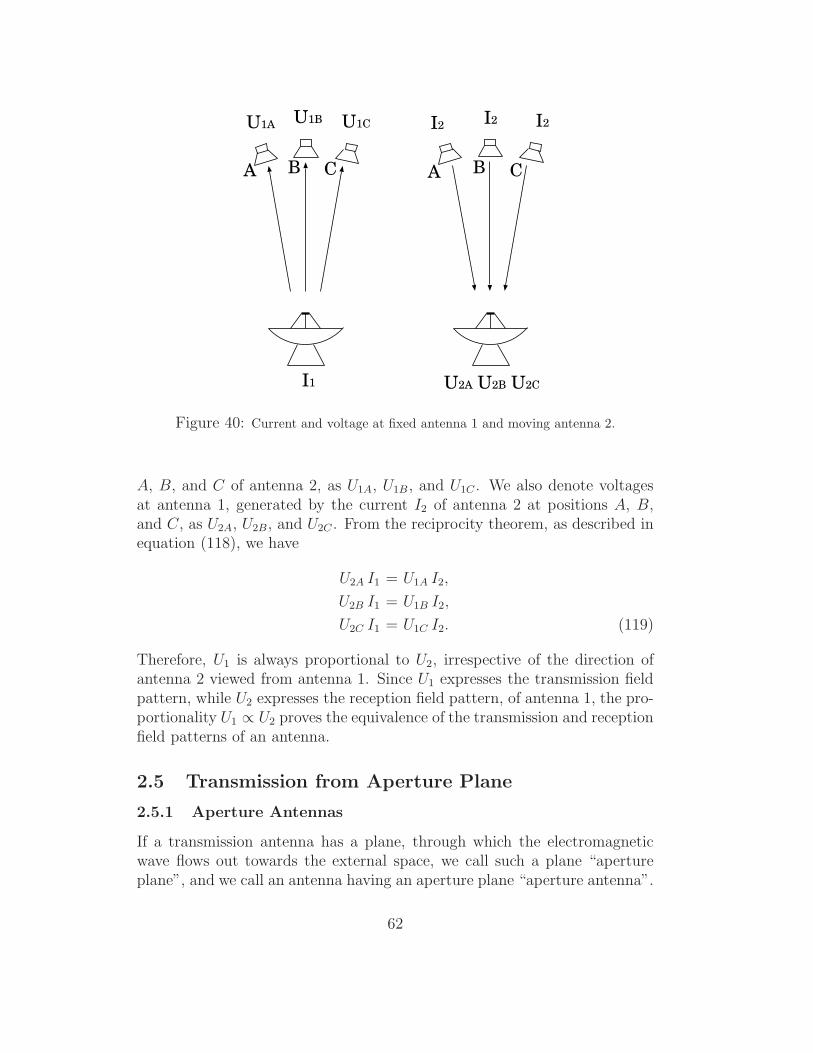
A B C

I1

U1A U1B U1C

A B C

U2A U2B U2C

I2 I2 I2

Figure 40: Current and voltage at fixed antenna 1 and moving antenna 2.

A, B, and C of antenna 2, as U1A, U1B , and U1C . We also denote voltagesat antenna 1, generated by the current I2 of antenna 2 at positions A, B,and C, as U2A, U2B, and U2C . From the reciprocity theorem, as described inequation (118), we have

U2A I1 = U1A I2,

U2B I1 = U1B I2,

U2C I1 = U1C I2. (119)

Therefore, U1 is always proportional to U2, irrespective of the direction ofantenna 2 viewed from antenna 1. Since U1 expresses the transmission fieldpattern, while U2 expresses the reception field pattern, of antenna 1, the pro-portionality U1 ∝ U2 proves the equivalence of the transmission and receptionfield patterns of an antenna.

2.5 Transmission from Aperture Plane

2.5.1 Aperture Antennas

If a transmission antenna has a plane, through which the electromagneticwave flows out towards the external space, we call such a plane “apertureplane”, and we call an antenna having an aperture plane “aperture antenna”.

62

As an example, let us consider a transmitting horn antenna, such as shownin Figure 41. Primary wave source (the oscillating current in the co–axial

A(aperture plane)

Figure 41: A horn antenna and an aperture plane.

to waveguide converter) is located in the waveguide tube, and generates theelectromagnetic fields in the horn. Then, the electromagnetic fields flow outof the horn towards the external space, through a plane A. This is theaperture plane, and the horn antenna is an aperture antenna. Parabololdal

aperture plane

Figure 42: A paraboloidal antenna and an aperture plane.

antennas are also typical aperture antennas (Figure 42).On the other hand, the linear dipole antenna such as shown in Figure 33

is not an aperture antenna.In order to consider the field transmission pattern of an aperture antenna,

it is convenient to regard, as if the electromagnetic waves are generated bysome fictitious wave source located on the aperture plane (Figure 43). Sucha “secondary wave source” can be uniquely related to the electromagnetic

63

E2

H2

primary source

E2

H2

secondary source

E1

H1

E1=0H1=0

Figure 43: Electromagnetic wave, transmitted from an aperture antenna (Left), can berepresented as a wave generated by an appropriately chosen secondary wave source on theaperture plane (Right).

field generated by the primary wave source, the actual oscillating currentwithin the feed horn, and can exactly reproduce the actual field transmissionpattern, as we will see below. The secondary source on an aperture planecan be interpreted in terms of Huygens and Fresnel’s principle, which states“each point on a primary wavefront can be considered to be a new source ofa secondary wave”.

2.5.2 Boundary Conditions on the Aperture Plane“Magnetic Current” and “Magnetic Charge”

N

ε1, µ1, σ1

E1, H1, D1, B1

ε2, µ2, σ2

E2, H2, D2, B2

Region 1

Region 2

Figure 44: Regions with different electromagnetic properties.

If physical properties of a medium are discontinuous at some boundarysurface, we solve physical equations on the both sides of the boundary, and

64

then connect the solutions, using a set of boundary conditions. The boundaryconditions for electromagnetic fields E1, H1, D1, B1 and E2, H2, D2, B2

in two regions with different ǫ1, µ1, σ1 and ǫ2, µ2, σ2, where ǫ, µ, and σare permittivity, permeability, and specific conductivity, correspondingly, arewell known: at a boundary surface, which separates the two regions, with aunit normal vector N (Figure 44), we have

N × (H2 − H1) = K, (120)

N × (E2 − E1) = 0, (121)

N · (D2 − D1) = Σ, (122)

N · (B2 − B1) = 0, (123)

where K [A m−1] is the surface density of electric current (or “surface electriccurrent”), and Σ [A s m−2] is the surface density of electric charge (or “surfaceelectric charge”).

However, having these usual boundary conditions alone is not sufficientto fulfil the requirements for the secondary source on the aperture plane, asshown in Figure 43, where E1 = 0 and H1 = 0 in the inner side of theaperture plane, while E2 6= 0 and H2 6= 0 in the outer side of the apertureplane.

In order to overcome this difficulty, we introduce virtual quantities called“magnetic current density” Jm, with unit [V m−2], and “magneticcharge density” ρm, with unit [V s m−3], following Adachi (S. Adachi,Electromagnetic Wave Engineering, 1985). They are supposed to be relatedwith the electromagnetic field quantities through “extended” Maxwell equa-tions:

∇× E = −Jm − ∂B

∂t, (124)

∇ · B = ρm, (125)

and to fulfil following boundary conditions:

N × (H2 − H1) = 0, (126)

N × (E2 − E1) = −Km, (127)

N · (D2 − D1) = 0, (128)

N · (B2 − B1) = Σm, (129)

where Km [V m−1] is the surface density of magnetic current (or “surfacemagnetic current”), and Σm [V s m−2] is the surface density of magneticcharge (or “surface magnetic charge”).

65

Note that an equation of continuity:

∂ρm

∂t+ ∇ · Jm = 0, (130)

holds in view of equations (124) and (125).Before discussing the boundary conditions at the aperture plane, let us

first consider a closed surface surrounding a primary wave source (Figure45). If we assume that the medium is continuous across the surface, the

E1, H1

E2, H2

E1 = 0, H1 = 0

primary wave source secondary wave source

E2, H2E2, H2

J

Figure 45: A closed surface surrounding a primary wave source (Left), which can beregarded as a secondary wave source with suitable surface currents and surface charges(Right).

electromagnetic fields must be also continuous, i.e. conditions E1 = E2,H1 = H2, D1 = D2 and B1 = B2 must hold on the surface.

Now, suppose we place surface electric current K, surface magnetic cur-rent Km, surface electric charge Σ and surface magnetic charge Σm on thesurface, which satisfy

K = N × H1, (131)

Km = −N × E1, (132)

Σ = N · D1, (133)

Σm = N · B1, (134)

where N is a unit normal vector, perpendicular to the surface. And then,we remove the primary wave source, and set the electromagnetic fields insideof the closed surface to zero, i.e. E1 = 0, H1 = 0, D1 = 0 and B1 = 0. Of

66

course, the electromagnetic fields become discontinous at the surface, in thiscase.

Let us compare boundary conditions at the surface in two cases, one withthe real continuous fields, and another with the fictitious discontinuous fields,together with the surface currents and the surface charges on the boundary.They are

Continuous fields case Discontinuous fields case

N × H2 = N × H1, N × H2 = K,

N × E2 = N × E1, N × E2 = −Km,

N · D2 = N · D1, N · D2 = Σ,

N · B2 = N · B1, N · B2 = Σm. (135)

As long as we consider these relations as boundary conditions at the closedsurface for external solutions of the electromagnetic fields, the left side con-ditions and the right side conditions are just equivalent to each other, inview of eauations from (131) to (134). Therefore, the external fields must beidentical for these two sets of boundary conditions. This implies that we cancalculate the external fields, provided that the appropriate surface currentsand surface charges, including both electric and magnetic, are given on theclosed boundary surface.

The same statement must be valid for the aperture plane, if the apertureplane is the only part of a closed surface surrounding the primary wave sourcethrough which the electromagnetic fields flow out.

Of course, we do not observe any magnetic current and magnetic chargein the real world, at least at present. It is interesting to note that equations(124) and (125) would really hold, if hypothetical magnetic monopoles exist.Although search for magnetic monopoles is one of the most exciting Topicsin the modern physics, no firm detection of monopoles has been reportedin the present level of technology (see, for example, an interesting article onthis matter by B. Schwarzschild in Physics Today, July, 2006). In the presentdiscussion, we use the magnetic current and the magnetic charge as auxiliaryconcepts, which help us to fulfil the requirements at the aperture plane, butleave no trace in our final results, as we will see later.

2.5.3 Wave Equations with Magnetic Current and Magnetic Charge

How can we calculate external electromagnetic fields when the surface cur-rents and the surface charges are given at a surface?

67

In order to answer to this question, we will first consider the wave gener-ations from the electric current & charge system, which we have seen before,and from the magnetic current & charge system, which are new for us, inparallel.

Electric Current & Charge System Magnetic Current & Charge System

Maxwell equations

∇× E = −∂B∂t

, ∇× E = −Jm − ∂B

∂t

∇× H = J +∂D

∂t, ∇× H =

∂D

∂t,

∇ · D = ρ, ∇ · D = 0,

∇ · B = 0, ∇ · B = ρm.

Equation of continuity

∂ρ

∂t+ ∇ · J = 0,

∂ρm

∂t+ ∇ · Jm = 0.

Electromagnetic potentials

B = ∇× A, D = −∇× Am,

E = −∇Φ − ∂A

∂t, H = −∇Φm − ∂Am

∂t.

Lorentz gauge

∇ · A + ǫ µ∂Φ

∂t= 0, ∇ · Am + ǫ µ

∂Φm

∂t= 0.

Wave equations with source terms

∇2A − 1

c2∂2A

∂t2= −µJ , ∇2Am − 1

c2∂2Am

∂t2= −ǫJm,

∇2Φ − 1

c2∂2Φ

∂t2= −1

ǫρ, ∇2Φm − 1

c2∂2Φm

∂t2= −1

µρ.

Retarded potentials with harmonically oscillating sources

A(r, t) = A(r)e−iωt, Am(r, t) = Am(r)e−iωt,E(r, t) = E(r)e−iωt, H(r, t) = H(r)e−iωt.

(J = 0, Jm = 0, ρ = 0, and ρm = 0, outside of the source region)

68

A(r) =µ

4π

∫

J(r′)eik|r−r′|

| r − r′ | dV′, Am(r) =

ǫ

4π

∫

Jm(r′)eik|r−r′|

| r − r′ | dV′,

H(r) =1

µ∇× A(r), E(r) = −1

ǫ∇× Am(r),

E(r) = ic

k∇× (∇× A(r)), H(r) = i

c

k∇× (∇× Am(r)).

Far field solutions in Fraunhofer region

T (n) =

∫

J (r′)e−ikn·r′

dV ′, T m(n) =

∫

Jm(r′)e−ikn·r′

dV ′,

A(r) =µ

4π

eikr

rT (n), Am(r) =

µ

4π

eikr

rT m(n),

H(r) = i1

2λ

eikr

rn × T (n), E(r) = −i 1

2λ

eikr

rn × T m(n),

E(r) = −i Z2λ

eikr

rn × [n × T (n)], H(r) = −i 1

2λZ

eikr

rn × [n × T m(n)].

Since the vector and scalar potentials are related to each other by Lorentzgauge relations, we considered here wave generations for vector potentialsA(r, t) and Am(r, t) only, as we did before.

In a case when both the electric current and the magnetic current co–exist, the electromagnetic fields are expressed by the superposition of twosets of solutions shown above. In the far field region, for example, we have

H(r) = i1

2λ

eikr

r

n × T (n) − 1

Zn × [n × T m(n)]

, (136)

E(r) = −i Z2λ

eikr

r

n × [n × T (n)] +1

Zn × T m(n)

. (137)

For these spherical waves in the far field region, we again obtain:

n · H = 0, and n · E = 0, (transversal wave),

and

E = −Z n × H , and H =1

Zn × E, (E, H orthogonal).

2.5.4 Radio Wave Transmission from a Surface

Now, how to describe the generation of electromagnetic waves from the sur-face electronic current K and the surface magnetic current Km on a surfaceof the secondary wave source?

69

dS

dl

l

N

N

K, Km

K, Km

Figure 46: A volume density of a surface density.

For this purpose, let us consider “a volume density of a surface density” ona boundary surface. Let a unit normal vector, perpendicular to the boundarysourface, be N . Let us consider a local rectangular coordinate system at acertain point on the surface, which are composed of an axis parallel to N andother two axes in a plane tangential to the boundary surface. If we denotethe length along N direction as l, and an infinitesimal surface area elementon the boundary as dS, then we can express an infinitesimal volume elementat the boundary as

dV = dl dS.Then, we can express the “volume densities” J and Jm of the surface den-sities K and Km as

J = K δ(l − l0),

Jm = Km δ(l − l0), (138)

where l = l0 corresponds to the boundary surface, and δ(x) is the deltafunction. Indeed, if we integrate the volume densities through a small volume∆V = ∆l∆S, containing a part of the boundary surface l = l0, we have

∫

∆V

J dV =

∫

∆V

Kδ(l − l0) dl dS =

∫

∆S

K dS,

∫

∆V

Jm dV =

∫

∆V

Kmδ(l − l0) dl dS =

∫

∆S

Km dS, (139)

as expected.Therefore, using equations (138) at every small element of the bound-

ary surface, we can express the retarded vector potentials generated by the

70

currents localized at the boundary as

A(r, t) =µ

4πe−iωt

∫

J (r′)eik|r−r′|

| r − r′ | dV ′ =µ

4πe−iωt

∮

K(r′)eik|r−r′|

| r − r′ | dS′,

Am(r, t) =µ

4πe−iωt

∫

Jm(r′)eik|r−r′|

| r − r′ | dV ′ =µ

4πe−iωt

∮

Km(r′)eik|r−r′|

| r − r′ | dS′,

(140)

where surface integrals are taken over the whole boundary surface.For the far field solutions, we have

T (n) =

∮

K(r′)e−ikn·r′

dS′,

T m(n) =

∮

Km(r′)e−ikn·r′

dS′, (141)

A(r, t) =µ

4π

ei(kr−ωt)

rT (n),

Am(r, t) =µ

4π

ei(kr−ωt)

rT m(n), (142)

and

H(r, t) = i1

2λ

ei(kr−ωt)

r

n × T (n) − 1

Zn × [n × T m(n)]

,

E(r, t) = −i Z2λ

ei(kr−ωt)

r

n × [n × T (n)] +1

Zn × T m(n)

, (143)

where n is a unit vector along the direction of the propagation of the sphericalwave, as before.

Comparing these equations with equations (136) and (137), we see thattheir forms are the same, and only difference is in the replacement of the vol-ume integrals in the expressions of T (n) and T m(n) by the surface integralasin equations (141).

Remembering here that the surface electric current and the surface mag-netic current must equal to

K = N × H1,

Km = −N × E1,

on the boundary surface with a unit normal vector N , in view of equations(131) and (132), we can rewrite T (n) and T m(n) in equations (141) as

T (n) =

∮

K(r′)e−ikn·r′

dS′ =

∮

N ×H1(r′)e−ikn·r′

dS′,

T m(n) =

∮

Km(r′)e−ikn·r′

dS′ = −∮

N ×E1(r′)e−ikn·r′

dS′. (144)

71

Now we have no longer the fictitiuous magnetic current in the right hand sideof equation (144), and the external electromagnetic fields in equations (143)are completely determined by the electromagnetic fields on the boundarysurface. This is a clear expression of Huygens and Fresnel’s principle thatthe wave front becomes the wave source.

2.5.5 Radio Wave Transmission from an Aperture Antenna

Let us consider an aperture antenna, with an aperture plane much larger insize than the wavelength. It is then possible to control the primary wavesource in such a way that harmonically oscillating electromagnetic fields onthe aperture plane, Ha and Ea, satisfy conditions:

N · Ha = 0, N · Ea = 0, (parallel to the aperture plane),

and

Ha =1

ZN × Ea, (mutually orthogonal), (145)

where N is the unit normal vector, perpendicular to the aperture plane(Figure 47). This corresponds to the case when the electromagnetic fields on

H

E

N

Figure 47: Electromagnetic field on an aperture plane.

the aperture plane are close to plane waves propagating towards the directionperpendicular to the aperture plane.

We now apply these relations to calculate directional pattern vectors T (n)and T m(n) in equations (144). Generally speaking, the surface integrals inequations (144) must be taken over a closed surface, surrounding the primarywave source. However, as we saw earlier, the closed surface can be replacedby the aperture plane A, if the aperture plane is the only part of a closed

72

surface through which the electromagnetic fields flow out. This condition isusually fulfilled in aperture antennas with aperture sizes much larger thanthe wavelengths (Figure 48).

AS

N

H, E

Figure 48: In an aperture antenna with aperture size much larger than the wavelength,most of the generated electromagnetic fields flow out through the aperture plane A. Inthis respect, the contribution of other portion S of the closed surface, surrounding theantenna, is negligibly small compared with that of the aperture plane A.

Therefore, we can rewrite equations (144) as

T (n) =

∫

A

N ×Ha e−ikn·r′

dS′ =1

Z

∫

A

N × (N ×Ea) e−ikn·r′

dS′,

T m(n) = −∫

A

N ×Ea e−ikn·r′

dS′, (146)

where, in the upper equation, we used an assumed property of the electro-magnetic fields on the aperture plane, given in equations (145).

Now, we obtain the far field solution of the electric field E(r, t), trans-mitted from an aperture antenna, by inserting equations (146) into one ofthe equations (143) and using one of the conditions on the aperture plane,given in equations (145):

E(r, t) = −i 1

2λ

ei(kr−ωt)

r

∫

A

n×n× [N ×(N ×Ea)]−N ×Ea e−ikn·r′

dS ′.

(147)For large aperture antennas, the electric field in the far field region has finitestrength only when the direction n is close enough to the direction N per-pendicular to the aperture plane. Therefore, we approximately take n = N

everywhere, except for in the argument of the exponential function. Then,using a formula of the vector algebra in equation (14), we obtain an equation:

E(r, t) = −i 1

λ

ei(kr−ωt)

r

∫

A

Ea(r′) e−ikn·r′

dS ′, (148)

which describes a relationship between electric fields on an aperture planeand in a spherical wave in the far field region.

73

2.5.6 Aperture Illumination and Field Pattern of an ApertureAntenna

In equation (148), the directional characteristics of the aperture antenna aresolely determined by the integral:

∫

A

Ea(r′) e−ikn·r′

dS′.

Regarding the distribution of the electric field Ea(r′) on the aperture plane,

Figure 49: Harmonically oscillating electric field on the aperture plane, keeping a com-mon field direction.

we assume that the electric field is parallel, and keep a constant direction,everywhere (Figure 49). This corresponds to a case of the linearly polarizedoscillation. If the actual field distribution is a superposition of different po-larization components, for example, a circularly polarized oscillation, whichcan be decomposed into two linearly polarized oscillations along two mutu-ally perpendicular directions, this discussion is valid for a linear polarizationcomponent along a certain direction.

Let us express, in this case, the electric field on the aperture plane as

Ea(r′) = E0 g(r

′), (149)

where E0 is a constant real vector, and g(r′) is a complex (in general) functionof the position on the aperture plane. The function g(r′) is called “apertureillumination”. This shows how the primary wave source (for example, afeed horn), like a flashlight, “illuminates” the aperture plane. Using theaperture illumination, we can rewrite equation (148) in a form:

E(r, t) = −iE0 λei(kr−ωt)

rf(n),

where

f(n) =

∫

A

g(r′) e−ikn·r′ dS′

λ2. (150)

74

The non–dimensional function f(n) is the field pattern of the aperture an-tenna in the far field region, which shows the directional characteristics ofthe generated electric field.

Taking into account that k = 2π/λ, and formally extending the area ofthe integration to an infinite plane, by just assuming that g(r′) = 0 outsideof the aperture plane A, we obtain, from equation (150),

f(n) =

∫

g(r′) e−i2πn·r′

λdS ′

λ2. (151)

This equation shows that the aperture illumination g(r′) and the field patternin the far field region f(n) of the aperture antenna form a two dimensionalspatial Fourier transform pair.

2.5.7 Power Pattern of an Aperture Antenna

We can now derive the power pattern of an aperture antenna by calculatingtime–averaged Poynting vector, as we did for the Hertz dipole.

We saw in equation (97) that the Poynting vector S of the spherical waveis described as

S = Er × Hr =1

Zn | Er |2,

where Er is the real part of the complex form of the electric field, whichrepresents the real physical quantity. Introducing the amplitude | f(n) | andthe phase φ of the complex field pattern f(n), we have

f(n) =| f(n) | eiφ. (152)

Then, from equation (150), we obtain

Er = ℜE(r, t) = E0 λ| f(n) |

rsin(kr − ωt+ φ). (153)

Since the time–averaged squared sine function always gives

sin2(kr − ωt+ φ) =1

2,

where ( ) denotes time averaging, we have

| S | =1

2Z| E0 |2

λ2

r2| f(n) |2. (154)

The non–dimensional term | f(n) |2 in equation (154) characterizes direc-tional pattern of the transmitted power, and can be regarded as power pat-tern P (n) in the far field region of an aperture antenna, though sometimes

75

| S | itself is called power pattern. In practice, “normalized power pat-tern” Pn(n), which is obtained by dividing the power pattern by its max-imum value, is used more frequently than the power pattern. Thus, thenormalized power pattern in the far field region of an aperture antenna isgiven by a formula:

Pn(n) =P (n)

Pmax=

| f(n) |2

| fmax |2, (155)

which is not affected by the difference of the two definitions of the powerpattern, mentioned above.

2.5.8 Main Lobe, Sidelobes, HPBW and BWFN

A typical normalized power pattern of an aperture antenna is illustrated inFigure 50. Left panel shows a rectangular plot, with horizontal axis show-ing angle from the “aperture axis” in radian. The aperture axis is an axisperpendicular to the aperture plane, which is usually parallel to the “beamaxis”, i.e., the direction of the maximum power pattern. Right panel showsa polar plot, which gives more realistic view of the pattern shape.

0

0.1

0.2

0.3

0.4

0.5

0.6

0.7

0.8

0.9

1

-1 -0.5 0 0.5 1

angle from aperture axis (radian)

norm

aliz

ed p

ower

pat

tern

HPBW

BWFN

Main lobe

Side lobes

Side lobes

Main lobe

Aperture axis

HPBW

BWFN

Figure 50: A normalized power pattern of an aperture antenna in a rectangular plot(Left) and in a polar plot (Right).

76

In both panels, a large main lobe (or main beam) is prominent. Thereare small sidelobes in both sides of the main lobe.

Two quantities are frequently used as measures of the width of the mainlobe, which is an important characteristic of an aperture antenna. One is“full half power beam width”, or HPBW, which stands for the twice ofthe angle of a direction, where the power pattern takes a half of the maximumvalue, from the aperture axis. Another is “full beam width between firstnulles”, or BWFN, which stands for the twice of the angle of a direction,where the power pattern drops to zero between the main lobe and the firstsidelobe, from the aperture axis (Figure 50).

2.5.9 Uniformly Illuminated Rectangular Aperture Antenna

Let us consider, as one of the simplest examples of aperture antennas, arectangular aperture antenna with an aperture plane located in xy–plane,which is uniformely illuminated as:

g(x, y) =

g for | x |≤ Lx

2, and | y |≤ Ly

2,

0 otherwise,(156)

where g is a real constant (see Figure 51).

x

y

Ly

Lx

nN

Figure 51: A rectangular aperture antenna.

From equation (151), the field pattern in the far field region f(n), in adirection of a unit vector n, with components nx and ny in the xy–plane, is

77

expressed in this case as

f(n) =

∫ ∫

g(x, y)e−i2π(nxx+nyy)/λdx

λ

dy

λ= g

Ly2

∫

−Ly2

Lx2

∫

−Lx2

e−i2π(nxx+nyy)/λ dx

λ

dy

λ

= gsin(πnxLx/λ)

πnx

sin(πnyLy/λ)

πny

. (157)

Since this function takes the maximum value (Lx/λ)(Ly/λ) when n = N (ornx = 0, ny = 0), where N is the unit vector normal to the aperture plane,the normalized power pattern as given in equation (155), is

Pn(n) =| f(n) |2

| fmax |2=

[

sin(πnxLx/λ)

πnxLx/λ

sin(πnyLy/λ)

πnyLy/λ

]2

. (158)

Full beam width between first nulls and full half power beam width of suchan antenna are

BWFN = 2 (λ

Lx

andλ

Ly

) (rad) = 114.6 (λ

Lx

andλ

Ly

),

and

HPBW = 0.88 (λ

Lxand

λ

Ly) (rad) = 50.4 (

λ

Lxand

λ

Ly), (159)

respectively.

2.5.10 Circular Aperture Antenna

Now let us consider a circular aperture antenna with diameter D, as shown inFigure 52. Let us assume an axisymmetric illumination around the apertureaxis, which is directed towards a unit vector N , perpendicular to the apertureplane, and let us choose a coordinate system, in which a directional unitvector n and a radius vector r′ within the aperture plane are given as

n ∼= (−u, 0, 1), (160)

andr′ = (λρ cosφ, λρ sinφ, 0), (161)

where λ is the wavelength, and ρ and φ are radial and azimuthal variables.If we denote the axisymmetric aperture illumination as

g(r′) = g(ρ), (162)

78

u

r’

nN

D

φ λρ

x

y

Figure 52: A circular aperture antenna.

then, according to equation (151), the field pattern at the direction n isdescribed in a form:

f(u) =

2π∫

0

∞∫

0

g(ρ) ei2πuρ cos φρdρdφ. (163)

Since Bessel function of zeroth order J0(z) is defined as

J0(z) =1

2π

2π∫

0

eiz cos φdφ, (164)

the field pattern is given by

f(u) = 2π

∞∫

0

g(ρ)J0(2πuρ)ρdρ. (165)

Therefore, according to equation (155), the normalized power pattern is

Pn(u) =

∞∫

0

g(ρ)J0(2πuρ)ρdρ

∞∫

0

g(ρ)ρdρ

2

. (166)

79

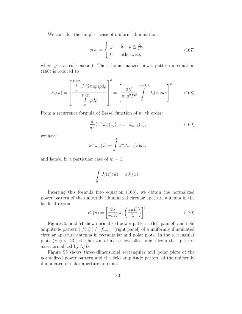
We consider the simplest case of uniform illumination:

g(ρ) =

g for ρ ≤ D2λ,

0 otherwise,(167)

where g is a real constant. Then the normalized power pattern in equation(166) is reduced to

Pn(u) =

D/2λ∫

0

J0(2πuρ)ρdρ

D/2λ∫

0

ρdρ

2

=

2λ2

π2u2D2

πuD/λ∫

0

J0(z)zdz

2

. (168)

From a recurrence formula of Bessel function of m–th order:

d

dzzmJm(z) = zmJm−1(z), (169)

we have

xmJm(x) =

x∫

0

zmJm−1(z)dz,

and hence, in a particular case of m = 1,

x∫

0

J0(z)zdz = xJ1(x).

Inserting this formula into equation (168), we obtain the normalizedpower pattern of the uniformly illuminated circular aperture antenna in thefar field region:

Pn(u) =

[

2λ

πuDJ1

(

πuD

λ

)]2

. (170)

Figures 53 and 54 show normalized power patterns (left pannel) and fieldamplitude pattern | f(u) | / | fmax | (right panel) of a uniformly illuminatedcircular aperture antenna in rectangular and polar plots. In the rectangularplots (Figure 53), the horizontal axes show offset angle from the apertureaxis normalized by λ/D.

Figure 55 shows three–dimensional rectangular and polar plots of thenormalized power pattern and the field amplitude pattern of the uniformlyilluminated circular aperture antenna.

80

0

0.2

0.4

0.6

0.8

1

-4 -2 0 2 4

Offset Angle Normalized by lambda/D

Normalized Power Pattern of Circular Aperture Antenna

0

0.2

0.4

0.6

0.8

1

-4 -2 0 2 4

Offset Angle Normalized by lambda/D

Normalized Field Pattern of Circular Aperture Antenna

Figure 53: Rectangular plots of normalized power pattern (Left) and field amplitudepattern (Right) of a uniformly illuminated circular aperture antenna. Horizontal axesshow offset angle from the aperture axis normalized by λ/D.

0

0.2

0.4

0.6

0.8

1

-0.2 -0.15 -0.1 -0.05 0 0.05 0.1 0.15 0.2

Polar Plot

Normalized Power Pattern of Circular Aperture Antenna

0

0.2

0.4

0.6

0.8

1

-0.2 -0.15 -0.1 -0.05 0 0.05 0.1 0.15 0.2

Polar Plot

Normalized Field Pattern of Circular Aperture Antenna

Figure 54: Polar plots of normalized power pattern (Left) and field amplitude pattern(Right) of a uniformly illuminated circular aperture antenna.

81

Figure 55: Three–dimensional rectangular (Top) and polar (Bottom) plots of the nor-malized power pattern (Left) and the field amplitude pattern (Right) of a uniformly il-luminated circular aperture antenna. Sidelobes are hardly seen in the polar plot of thenormalized power pattern.

82

From numerical values of Bessel function J1(x), we obtain full beam widthbetween first nulls and full half power beam width of the uniformly illumi-nated circular aperture antenna as

BWFN = 2.44λ

D(rad) = 140

λ

D,

and

HPBW = 1.02λ

D(rad) = 58.4

λ

D, (171)

respectively.

2.6 Beam Patters of Aperture Antennas

So far, we have discussed and derived field and power patterns of aperture an-tennas in the transmission mode. Because of the equivalence of field patternsin transmission and reception, which we saw earlier, the field transmissionpattern must be the same with the field reception pattern. In the receptioncase, the field pattern is often called ‘voltage reception pattern’, as describingthe magnitude of the received voltage as a function of the antenna direction.

Since the transmitted power is proportional to the square of the electricfield, and the received power is proportional to the square of the receivedvoltage, the power reception pattern must also be equivalent to the powertransmission pattern.

The antenna beam pattern is a general concept, which means eitherthe power pattern or the field (or voltage–reception) pattern, depending onthe context.

2.6.1 Antenna–Fixed Coordinate System

For further convenience, let us introduce an ‘antenna–fixed coordinate sys-tem’ for a paraboloidal antenna.

As the origin of the coordinate system, we choose the center of theparaboloid surface of the main reflector. Then, let us take the aperture axis,or the symmetry axis of the paraboloid, as the polar axis z, and choose thex and y axes towards directions perpendicular and parallel to the elevationaxis, as shown in Figure 56. Finally, let us denote a given direction in thesky by an angle from the polar axis θ, and an azimuthal angle φ measuredfrom the x–axis towards the y–axis.

Then, the field pattern and power pattern can be described as functionsof these angles, such as f(θ, φ), and P (θ, φ). For example, we can definethe power pattern in the reception case as the power P (θ, φ) received by an

83

θ

φ

El axis

paraboloid axis

P(θ, φ)

z

x

y

Figure 56: Antenna–fixed coordinate system.

antenna from a point–like source of unit flux density at direction θ and φ.Similarly to the transmission case, the normalized power pattern is given by

Pn(θ, φ) =P (θ, φ)

Pmax

=| f(θ, φ) |2

| fmax |2. (172)

2.6.2 A Useful Formula: HPBW ≈ λ/D

From the two simple examples of the aperture antennas, which we saw earlier,it is evident that HPBW ∼= λ/D (see equations (159) and (171)). This isgenerally valid for a wide variety of aperture antennas with realistic apertureilluminations. Therefore, the ratio λ/D is often used as a measure of thebeam width, or the angular resolution, of radio telescope antennas (table 1).

Of course, it is not an easy task to direct a huge radio telescope with45 m diameter, say, towards an astronomical object with an accuracy muchbetter than 0.0025 degree!

2.6.3 Distance to Fraunhofer Region

As we saw earlier, the antenna beam pattern is a function of distance fromthe antenna in the Fresnel region, or in the near field, as schematically shown

84

diameter D wavelength λ frequency ν λ/D

6 m 37.5 mm 8 GHz 0.36

10 m 7.0 mm 43 GHz 0.04

21 m 2.3 mm 129 GHz 0.0063

45 m 2.0 mm 150 GHz 0.0025

Table 1: Beam widths (λ/D ≈ HPBW) of antennas with different aperture diameters,observing at different frequencies.

in Figure 57 (Adachi, Electromagnetic Wave Engineering, 1985).

Figure 57: Variation of the electric field amplitude pattern with distance from theantenna (Adachi, Electromagnetic Wave Engineering, 1985).

However, in the Fraunhofer region, or in the far field, the beam patternbecomes almost independent of the distance, as illustraited by the rightmostcurve of Figure 57.

For a paraboloidal antenna, we can use the aperture diameter as the char-acteristic size of the wave source region in the Fraunhofer condition given in(89). Therefore, the ‘distance to the Fraunhofer region’ rF for a paraboloidal

85

r

D

λ16

aperture plane

p

r’

Figure 58: Distance to the Fraunhofer region as a condition for the plane wave approx-imation of the received wave.

antenna, with the aperture diameter D, receiving or transmitting a radiowave with wavelength λ, is given by

rF ≡ 2D2

λ. (173)

The Fraunhofer condition r ≫ rF can be graphically illustrated as thecondition where the difference between the distance from a distant point pto the edge of the aperture r′, and that to the center of the aperture r,must be much smaller than λ/16 (Figure 58). This could be interprettedas a condition, that a spherical wave coming from the distant point can bepractically approximated as a plane wave.

rW=rF / 2

DHPBW

Figure 59: Distance to the Fraunhofer region as a condition for predominance of thefar–field beam in the transmitted wave.

Also, rF is equal to the twice of the distance rw to a point, where thewidth of the far–field beam, measured at HPBW, becomes equal to the width

86

D λ rF = 2D2/λ

6 m 3.8 cm ( 8 GHz) 1.9 km

10 m 7 mm ( 43 GHz) 28.6 km

21 m 2.3 mm (129 GHz) 383 km

45 m 2 mm (150 GHz) 2025 km

2300 km 7 mm ( 43 GHz) 1.51 × 1012 km

VLBI = 0.16 light year

Table 2: Distances to the Fraunhofer region.

of a circular cylinder with the diameter of the aperture D, i.e.,

λ

Drw = D, and , hence, rw =

D2

λ=rF

2,

(Figure 59). This could be interpreted as a condition that most of the trans-mitted power is confined within the far–field beam.

Table 2 shows typical examples of the distances to the Fraunhofer region.Can we measure the far–field patterns of our antennas on the ground?

2.7 Illumination Taper (or Gradation)

We can modify antenna beams by changing the electric field distribution on

a

b

c

feed horn

aperture plane

main reflector

subreflector

Figure 60: Aperture illumination.

the aperture plane (the illumination pattern). Therefore, in order to realize

87

a desired beam pattern, we can design a feed horn, so that the horn suitably‘illuminates’ the aperture plane (Figure 60).

Generally speaking, it is desirable to have a beam pattern which wouldexhibit as narrow as possible main lobe and as low as possible sidelobe level.However, these two requirements are somewhat in conflict, as illustratedbelow.

Figure 62 shows field patterns in the far–field region normalized by theirpeak values for circular aperture antennas with simple aperture illuminationpatterns. The field patterns are derived by equation (165) which is based onthe simple two–dimensional spatial Fourier transform relationship betweenthe illumination patterns and the field patterns.

We can see in the figure that the main lobe is narrowest when the aper-ture illumination is uniform. However, the sidelobe level is rather high inthe uniform illumination case. On the other hand, if we apply a Gaussianillumination, we get fairly low sidelobe level, but the main lobe becomesbroader.

The non–uniform illumination, which is stronger in the central part ofthe aperture, and weaker in the outer parts, is called ‘tapered’ or ‘gradated’illumination.

For radio telescopes, which receive very weak signals from astronomi-cal radio sources, the thermal radiation of the ground (with temperature ofT ≃ 300 K!) picked up by the sidelobes may seriously degrade the signal–to–noise (S/N) ratio. Likewise, the ground thermal radiation received from theoutside of the main reflector edge (which is called ‘spillover’ in the transmis-sion sense) is also quite harmful (Figure 61).

300 K

sidelobe pick up

spillover

main lobe

Figure 61: Why is strong tapering required for radio telescopes?

88

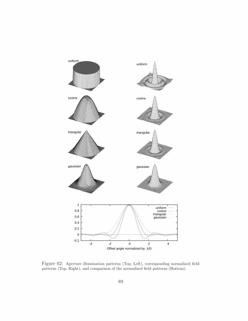
cosine

triangular

gaussian

uniform

cosine

triangular

gaussian

uniform

-0.2

0

0.2

0.4

0.6

0.8

1

-4 -2 0 2 4

Offset angle normalized by λ/D

uniformcosine

triangulargaussian

Figure 62: Aperture illumination patterns (Top, Left), corresponding normalized fieldpatterns (Top, Right), and comparison of the normalized field patterns (Bottom).

89

Therefore, rather strong tapering is required for radio telescopes, althoughthis of course means that we have to sacrifice some portion of their apertureareas as ‘ineffective’ areas.

2.8 Spectral Flux Density Received by an Antenna

Beam

We defined earlier that the spectral flux density Sν is a portion of the radi-ation energy from an astronomical source incoming through a cross sectionof unit area, per unit frequency bandwidth, and per unit time. The spectralflux density was described, through the monochromatic intensity Iν(θ, φ), byan integral over the source solid angle Ω:

Sν =

∫∫

Ω

Iν(θ, φ) cos θ sin θ dθ dφ,

where the cos θ term arose due to a geometrical effect corresponding to theprojection of a unit area onto the plane perpendicular to an incoming ray(left panel of Figure 63).

s

θ

∆σ

θ

∆σ

s

Figure 63: Flux density as received by a unit area in space (Left), and the effective fluxdensity as received by a unit area on the aperture plane of a directional antenna (Right).

On the other hand, an antenna with a normalized power pattern Pn(θ, φ)receives the radiation from the radio source in proportion to Pn(θ, φ), whichreflects not only the geometrical effect but also the electromagnetic effect.Therefore, the portion of the radiation energy received by a unit area on the

90

antenna aperture plane, per unit frequency bandwidth, and per unit time, isdescribed by

Sν =

∫∫

Ω

Pn(θ, φ) Iν(θ, φ) sin θ dθ dφ, (174)

where θ and φ are the angular variables in the antenna–fixed coordinatesystem (right panel of Figure 63). We call this ‘intensity collected by theantenna beam’ Sν in equation (174) the ‘effective flux density’. The effectiveflux density is equal to the usual total flux density when the angular sizeof the source is much smaller than the antenna beam width, and when thebeam is exactly directed towards the source. Otherwise, the effective flux issmaller than the total flux. Henceforth, we use the word ‘flux density’ in thesense of the effective flux density, as far as radio wave reception with radiotelescope antennas is concerned.

3 Antenna Characteristics

The performance of a radio wave antenna is characterized by a number ofimportant parameters which usually figure in specifications of the antenna.The major peerformance parameters include

• Aperture diameter,

• Frequency Range,

• Surface accuracy,

• Pointing accuracy,

• Antenna reference point,

• Antenna gain,

• Range of motion and slewing speed,

• Survival loads.

Examples of antenna specifications are shown in tables 3 and 4.We will introduce major performance characteristics of antennas, and

discuss meanings of numbers in the specifications. We will also discuss waysto estimate important charactersitics such as aperture efficiency, antennagain, and maximum observable frequency, on the basis of the specifications.

91

Optics Cassegrain focus, central feed type

Primary diameter 21 m

Primary focal length 7 m

Secondary diameter 2 m

Secondary focal length 37 cm

Mechanical operation Fast switching up to 2.5 separation

Azimuth range ±270

Elevation range 0 – 91

Az max. slew speed 3/s

El max. slew speed 3/s

Az max. acceleration ≥ 1/s2

El max. acceleration ≥ 1/s2

Surface accuracy Appropriate for reception at 150 GHz

Panels 65 µm rms

Total 150 µm rms (10 m/s wind)

Pointing performance Appropriate for reception at 150 GHz

Pointing accuracy 0.001 rms (10 m/s wind)

Az natural freq. 2.5 Hz

El natural freq. 2.5 Hz

Subref. spar nat. freq. 5 Hz

Az El axes offset 3 mm

Az El orthogonality 0.01

Operational loads Temperature -20C – 40C

Wind 10 m/s

Survival Loads Wind 90 m/s

Seismic acceleration 0.2 G horiz., 0.1 G vert.

Table 3: An example of specifications for an astrophysical VLBI antenna.

92

Aperture diameter 22 m

Frequency bands 2 GHz (S), 8 GHz (X), 22 GHz (K), 43 GHz (Q)

Polarization RHCP or LHCP selectable for all 4 bands

Surface accuracy ≤ 0.3 mm RMS (Panel ≤ 0.2 mm RMS)

Gain S: 51.0 dB, X: 63.0 dB, K: 71.7 dB, Q: 77.7 dB

Subreflector Accuracy ≤ 0.1 mm RMS, motorized hexapod

Pointing accuracy ≤ 0.0022 RMS (wind ≤ 10 m s−1)

Reference point Measurable from outside, invar tube along Az–axis

Az–axis verticality ≤ 0.0025

Az, El–axes orthogonality ≤ 0.0025

Az, El–axes offset ≤ 1.5 mm

Range of motion ± 270 in Az, 0 ∼ 90 in El

Slew speed max 5 s−1 in Az, max 5 s−1 in El

Operational wind load 15 m s−1

Survival wind load 70 m s−1

Foundation Mat foundation + concrete piles

Table 4: An example of specifications for a geodetic VLBI antenna.

93

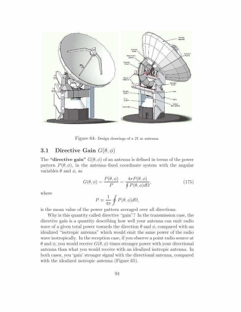
Figure 64: Design drawings of a 21 m antenna.

3.1 Directive Gain G(θ, φ)

The “directive gain” G(θ, φ) of an antenna is defined in terms of the powerpattern P (θ, φ), in the antenna–fixed coordinate system with the angularvariables θ and φ, as

G(θ, φ) =P (θ, φ)

P=

4πP (θ, φ)∮

P (θ, φ)dΩ, (175)

where

P ≡ 1

4π

∮

P (θ, φ)dΩ,

is the mean value of the power pattern averaged over all directions.Why is this quantity called directive “gain”? In the transmission case, the

directive gain is a quantity describing how well your antenna can emit radiowave of a given total power towards the direction θ and φ, compared with anidealized “isotropic antenna” which would emit the same power of the radiowave isotropically. In the reception case, if you observe a point radio source atθ and φ, you would receive G(θ, φ) times stronger power with your directionalantenna than what you would receive with an idealized isotropic antenna. Inboth cases, you ‘gain’ stronger signal with the directional antenna, comparedwith the idealized isotropic antenna (Figure 65).

94

P

P(θ,φ)

power pattern of isotropic antenna

power pattern ofdirectional antenna

Figure 65: Directive gain: “gain” of a directional antenna compared with an idealizedisotropic antenna.

3.2 Beam Solid Angle ΩA

The “beam solid angle” ΩA is another measure of the angular extent of theantenna beam, along with the HPBW and BWFN, defined by an equation:

ΩA =

∮

Pn(θ, φ)dΩ =

∮

P (θ, φ)dΩ

Pmax

=4πP

Pmax

, (176)

where Pn(θ, φ) is the normalized power pattern as defined in equation (155):

Pn(θ, φ) =P (θ, φ)

Pmax.

If we display the antenna power pattern in a rectangular plot, where the x–and y– coordinates are angles in two perpendicular directions in the apertureplane, and if we approximate the solid angle by an area in this xy– plane,the beam solid angle is equal to the cross–sectional area of a cylinder whichhas a height of Pmax, and the same “volume” as the power pattern in thisrectangular coordinate system (Figure 66).

3.3 Main Beam Solid Angle ΩM

The “main beam solid angle” is defined in a similar way to the beamsolid angle, but now the integration covers the main lobe only:

ΩM =

∫

main lobe

Pn(θ, φ)dΩ. (177)

95

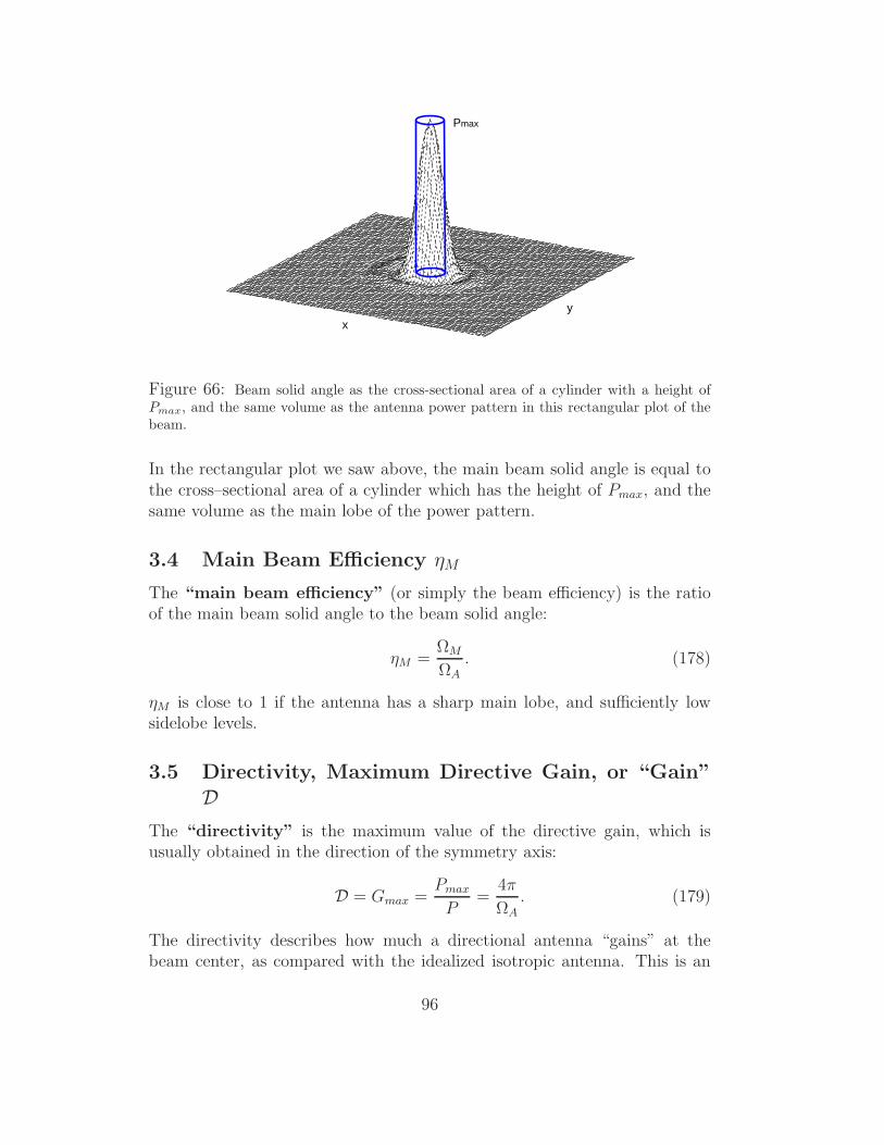
Pmax

x

y

Figure 66: Beam solid angle as the cross-sectional area of a cylinder with a height ofPmax, and the same volume as the antenna power pattern in this rectangular plot of thebeam.

In the rectangular plot we saw above, the main beam solid angle is equal tothe cross–sectional area of a cylinder which has the height of Pmax, and thesame volume as the main lobe of the power pattern.

3.4 Main Beam Efficiency ηM

The “main beam efficiency” (or simply the beam efficiency) is the ratioof the main beam solid angle to the beam solid angle:

ηM =ΩM

ΩA. (178)

ηM is close to 1 if the antenna has a sharp main lobe, and sufficiently lowsidelobe levels.

3.5 Directivity, Maximum Directive Gain, or “Gain”D

The “directivity” is the maximum value of the directive gain, which isusually obtained in the direction of the symmetry axis:

D = Gmax =Pmax

P=

4π

ΩA

. (179)

The directivity describes how much a directional antenna “gains” at thebeam center, as compared with the idealized isotropic antenna. This is an

96

important antenna parameter which is also called the “antenna gain”, orsimply “gain” (not to be confused with the “directive gain” G(θ, φ)).

The antenna gain is usually expressed in decibels (dB):

D (in dB or dBi) = 10 log10(Pmax

P), (180)

where log10 is the common (i.e. base 10) logarithm, and “dBi” here is thesame as dB but stresses that the comparison is made with the isotropic case.

3.6 Antenna Polarization

3.6.1 Some Notes on Polarization of Electromagnetic Wave

E

H

k

polarization plane of electric field

polarization plane of magnetic field

Figure 67: An electromagnetic wave as a polarized wave.

Since an electromagnetic wave is a transverse wave, as we saw in thediscussions of the plane and spherical waves, the electric or magnetic fieldvector in the wave oscillates along a certain direction within a plane which isperpendicular to the direction of the propagation, and moves with the wave(Figure 67). Such a wave is said to be “polarized”.

There are two degrees of freedom in the oscillation within the plane.Therefore, any wave with a certain direction of polarization can be ex-pressed as a linear combination of two independent polarization components.Such independent components could be two linearly polarized componentsin mutually orthogonal directions (horizontal and vertical, say) or two circu-larly polarized components with mutually opposite rotational senses (RHCP:Right Hand Circular Polarization, and LHCP: Left Hand Circular Polariza-tion), as shown in Figure 68.

3.6.2 Polarization Characteristics of Antennas

Any antenna (or, better to say, any waveguide to coaxial–cable converter)can receive or transmit only one independent component of the polariza-

97

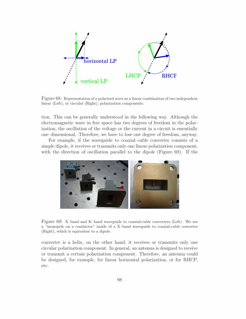
RHCPLHCP

horizontal LP

vertical LP

Figure 68: Representation of a polarized wave as a linear combination of two independentlinear (Left), or circular (Right), polarization components.

tion. This can be generally understood in the following way. Although theelectromagnetic wave in free space has two degrees of freedom in the polar-ization, the oscillation of the voltage or the current in a circuit is essentiallyone–dimensional. Therefore, we have to lose one degree of freedom, anyway.

For example, if the waveguide to coaxial–cable converter consists of asimple dipole, it receives or transmits only one linear polarization component,with the direction of oscillation parallel to the dipole (Figure 69). If the

Figure 69: X–band and K–band waveguide to coaxial-cable converters (Left). We seea “monopole on a conductor” inside of a X–band waveguide to coaxial-cable converter(Right), which is equivalent to a dipole.

converter is a helix, on the other hand, it receives or transmits only onecircular polarization component. In general, an antenna is designed to receiveor transmit a certain polarization component. Therefore, an antenna couldbe designed, for example, for linear horizontal polarization, or for RHCP,etc.

98

Of course, the antenna polarization can be relatively easily changed byadjusting the waveguide to coaxial–cable converter or using special opticaldevices. Moreover, one can install two or more waveguide to coaxial–cableconverters, and following receiving systems, in a common main–reflector andsub–reflector system in order to simultaneously receive or transmit the twopolarization components by “a single antenna” (which, in actuality, containstwo antennas in the strict sense of the second definition by Kraus).

The specification of the antenna polarization performance is usually givenas “polarization isolation”. This shows how well an antenna can receiveone polarization component, to which the antenna is designed, without be-ing contaminated by another component (often called as “cross-polarizationleakage”), which may arise due to some inperfection in the antenna optics.

3.6.3 Antenna Polarization and VLBI

In a majority of radio sources, two independent polarization components areonly very weakly correlated (“unpolarized sources”). Therefore, it is quiteimportant for VLBI observations that participating antennas observe radiosources in the same polarization mode, except in the cases when the weakcorrelation between different polarization components itself is the target ofstudy (“polarization observation”). Wrong setting of polarization has beenone of major sources of failures in VLBI observations.

It is not easy to use linear polarization antennas for VLBI observations,because the directions of the linear polarization fixed to antennas usuallycorrespond to different sky directions, and the difference varies in time asthe Earth rotates, for antennas located at different points on the Earth sur-face. Therefore, the VLBI antennas in the world are mostly designed toreceive circular polarization components. In geodetic VLBI, RHCP has beenconventionally used.

3.7 Effective Aperture Ae

Let us consider that the randomly polarized (or ‘unpolarized”) radio wave isincident to a radio telescope antenna. The word “unpolarized” here meansthat all kinds of waves with different polarization directions are randomlymixed up so that in average no net predominant polarization component isleft. Radio waves from most of the astronomical sources are known to bepractically unpolarized in this sense.

If an antenna receives a certain amount of power per unit frequency band-width Wν by observing a randomly polarized radio source with the effectiveflux density Sν , the “effective aperture” Ae of the antenna is defined by

99

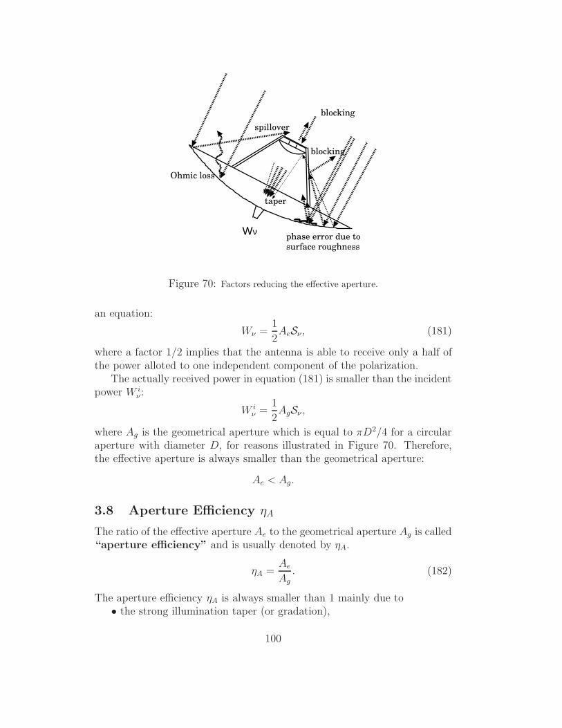
Wν

blocking

phase error due tosurface roughness

taper

spillover

Ohmic loss

blocking

Figure 70: Factors reducing the effective aperture.

an equation:

Wν =1

2AeSν , (181)

where a factor 1/2 implies that the antenna is able to receive only a half ofthe power alloted to one independent component of the polarization.

The actually received power in equation (181) is smaller than the incidentpower W i

ν :

W iν =

1

2AgSν ,

where Ag is the geometrical aperture which is equal to πD2/4 for a circularaperture with diameter D, for reasons illustrated in Figure 70. Therefore,the effective aperture is always smaller than the geometrical aperture:

Ae < Ag.

3.8 Aperture Efficiency ηA

The ratio of the effective aperture Ae to the geometrical aperture Ag is called“aperture efficiency” and is usually denoted by ηA.

ηA =Ae

Ag

. (182)

The aperture efficiency ηA is always smaller than 1 mainly due to• the strong illumination taper (or gradation),

100

• the phase error due to the roughness of the antenna surface,• the blocking by the subreflector and the stays,• the spillover from the subreflector,• the Ohmic dissipation on the surface,

as schematically illustrated in Figure 70.

3.9 Nyquist Theorem on Noise Power

In further discussions, we will often use an important theorem on the powerof the noise derived by Nyquist (1928).

Suppose that we have an electric circuit with a resistor of resistance Rwhich is in thermodynamical equilibrium with the environment of tempera-ture T (Figure 71).

Detector

Resistor

TR

i

i

t

Figure 71: Power generated by a resistor which is in thermodynamical equilibrium withthe environment of temperature T .

Then, we have electric current i in the circuit due to the thermal noise.Average of such noise current is usually zero: 〈i〉 = 0. But average of squareof the noise current is not, in general, zero: 〈i2〉 6= 0. So, we have some powerdue to the thermal noise.

According to the Nyquist Theorem (H. Nyquist, 1928, Phys. Rev., 32,110–113), the average noise power Wν per unit frequency bandwidth is givenby

Wν = kT, (183)

where k is Boltzmann constant (k = 1.381 × 10−23 J K−1), in the classicallimit hν ≪ kT .

We will briefly see how the theorem is derived following discussions byNyquist (1928).

Let us consider two conductors each of resistance R connected by a longnon–dissipative transmission line which has characteristic impedance R andsatisfies non–reflection condition at either end of the line (Figure 72). Letlength of the transmission line be l and propagation velocity be v. Let thesystem be in the thermodynamical equilibrium with temperature T .

101

R

T

R

T

l

v

Conductor 1 Conductor 2

Transmission line

v

Figure 72: Two conductors each of resistance R and in temperature T connected by adissipationless non–reflecting transmission line.

1. There are two trains of energy, one goes from left to right through thetransmission line corresponding to the power generated in conductor1 and absorbed in conductor 2, and another in the reverse direction.Under the thermodynamical equilibrium, the power flowing from con-ductor 1 to conductor 2 must be exactly equal to the power flowing fromconductor 2 to conductor 1 at any frequency bandwidth (otherwise thesecond law of thermodynamics is violated).

2. Suppose that we isolate the transmission line from the conductors byapplying short circuits at the two ends. Then complete reflection is setup at the ends and traveling waves in opposite directions are convertedto standing waves (normal mode oscillations with fixed ends). Thus,the energy of the noise current is trapped in the transmission line.

3. Eigen frequencies of the normal modes are

ν1 =v

2l, ν2 =

v

l, ν3 =

3v

2l, ν4 =

2v

l, · · · ,

corresponding to the fundamental tone and overtones (Figure 73). There-fore, the number of normal modes contained in a frequency bandwidthfrom ν to ν + ∆ν is (2l/v)∆ν.

4. In the classical limit (hν ≪ kT ), average energy per one normal modeoscillation is equal to kT in the thermodynamical equilibrium. One–half of this energy is magnetic and one–half is electric. (This is anal-ogous to the string oscillation case, where average kinetic energy perone degree of freedom under the thermodynamical equilibrium is equalto kT/2 according to the law of equipartition of energy, while kineticenergy is equal to potential energy in the oscillation, and hence averagetotal energy per one normal mode oscillation, is kT ).

102

ν1

ν2

ν3

ν4

Figure 73: Fundamental tone and overtones of normal mode oscillations of a string witheigenfrequencies ν1 = v

2l, ν2 = v

l, ν3 = 3v

2l, ν4 = 2v

l, · · · .

5. Therefore, the total energy contained in the frequency bandwidth fromν to ν + ∆ν is equal to (2l/v) kT ∆ν.

6. This amount of energy should have been transferred from the two con-ductors to the transmission line during the time of transit ∆t = (l/v)when the line was connected to the conductors. Consequently, the noisepower per unit bandwidth generated by one conductor Wν should be

Wν =1

2

1

∆t

1

∆ν

2l

vkT ∆ν = kT,

as given in equation (183).

In the energy region where the condition of the classical limit (hν ≪ kT )does not hold, the simple law of equipartition of the total energy kT per onenormal mode oscillation is no longer valid. For such a case, Nyquist (1928)gives a more general equation on power of the noise:

Wν =hν

ehνkT − 1

.

3.10 Effective Aperture and Beam Solid Angle

The effective aperture Ae and the beam solid angle ΩA are related with eachother through the wavelength λ by a simple equation:

AeΩA = λ2. (184)

103

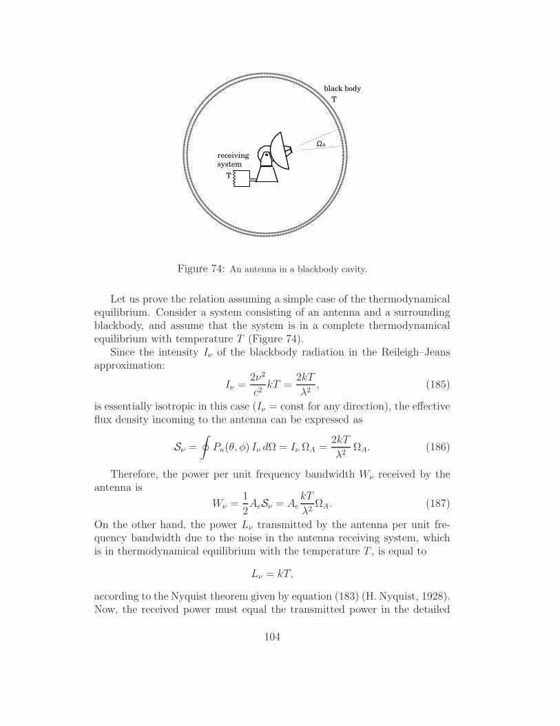
ΩA

T

T

black body

receivingsystem

Figure 74: An antenna in a blackbody cavity.

Let us prove the relation assuming a simple case of the thermodynamicalequilibrium. Consider a system consisting of an antenna and a surroundingblackbody, and assume that the system is in a complete thermodynamicalequilibrium with temperature T (Figure 74).

Since the intensity Iν of the blackbody radiation in the Reileigh–Jeansapproximation:

Iν =2ν2

c2kT =

2kT

λ2, (185)

is essentially isotropic in this case (Iν = const for any direction), the effectiveflux density incoming to the antenna can be expressed as

Sν =

∮

Pn(θ, φ) Iν dΩ = Iν ΩA =2kT

λ2ΩA. (186)

Therefore, the power per unit frequency bandwidth Wν received by theantenna is

Wν =1

2AeSν = Ae

kT

λ2ΩA. (187)

On the other hand, the power Lν transmitted by the antenna per unit fre-quency bandwidth due to the noise in the antenna receiving system, whichis in thermodynamical equilibrium with the temperature T , is equal to

Lν = kT,

according to the Nyquist theorem given by equation (183) (H. Nyquist, 1928).Now, the received power must equal the transmitted power in the detailed

104

balance of the thermodynamical equilibrium. Therefore,

Lν = Wν −→ AeΩA

λ2= 1 −→ AeΩA = λ2. (188)

Although we derived equation (184) in the thermodynamical equilibriumcase, the resultant equation does not contain any thermodynamical quantity.Therefore, the equation must generally hold in other cases as well.

3.11 Directivity D and Aperture Efficiency ηA

As we saw earlier, the directivity (or gain) D is related to the beam solidangle ΩA by equation (179):

D =4π

ΩA.

Now using equation (184), we can transform the above equation to

D = 4πAe

λ2= 4πηA

Ag

λ2, (189)

where Ag and λ are the geometrical aperture and the wave length, respec-tively.

For a circular aperture antenna with diameter D, we have

D = ηA

(

πD

λ

)2

. (190)

If the aperture efficiency ηA is kept nearly constant, we could obtain highergain with larger diameter and higher frequency. In actuality, however, itbecomes increasingly difficult to realize the high aperture efficiency as we goto the higher frequency and/or to the larger diameter.

In performance descriptions of antennas, the gain of an idealized antennawith 100 % aperture efficiency:

(

πD

λ

)2

, (191)

is often described as “100 % gain”, and usually given in dB. The 100 % gaincan be directly calculated from the aperture diameter D and the observingwavelength λ. Therefore, if we can estimate the aperture efficiency ηA, wecan easily get a value for the gain D, as we will examine later.

105

3.12 Illumination Taper and Aperture Efficiency

Rather strong illumination taper is required in radio telescope antennas toavoid undesired ground pickups due to the sidelobes or the spillover from themain reflector as we saw in Section 2.7. The strong taper lowers the sidelobelevel. At the same time, however, it increases the beam width as we saw inFigure 62. The increase of the beam width and therefore of the beam solidangle ΩA decreases the effective aperture Ae as required from equation (184):

Ae =λ2

ΩA.

In general, the illumination taper improves the main beam efficiency ηM

but deteriorates the aperture efficiency ηA. The illumination taper is oftenthe largest factor reducing the aperture efficiency of radio telescope antennasto the level of 50 – 60 %.

3.13 Surface Roughness and Aperture Efficiency

The surface roughness is another important factor which determines the aper-ture efficiency of radio telescope antennas.

Suppose that a real main reflector deviates from an ideal paraboloid dueto the roughness of its surface. Then, the rays, which originally formed awave front of equal phase in a plane wave, and were reflected at differentpoints on the main reflector, reach at the focus with different path lengths,and, therefore, with different phases, due to the surface roughness. Thus, therays reached at the focus are summed up with different phases. Therefore,the maximum power pattern Pmax at the center of the main lobe becomessomewhat lower than the one in the ideal paraboloid case with perfectlysmooth surface. On the other hand, the averaged power pattern P must notchange by the surface roughness, since the total power must be conserved.

Therefore, the directivity D = Pmax/P , and the effective aperture Ae =Dλ2/(4π), are reduced, compared with the ideal case. Because of the samereason, the reduced power in the main lobe must be balanced by an increasedpower in the sidelobes.

Thus, the surface roughness deteriorates both the aperture efficiency ηA

and the main beam efficiency ηM .Let us calculate how the aperture efficiency is reduced due to the sur-

face roughness of the main reflector, again in the transmission mode. Forsimplicity, we ‘stretch’ the actual paraboloid surface and treat it as a plane,parallel to the aperture plane, and regard that the rays are coming from adirection, perpendicular to the ‘main–reflector plane’, as shown in Figure 75.

106

εideal surface

real surface

ε2

aperture plane

Figure 75: Phase error due to the surface roughness.

This implies that a subreflector, and a primary feed, must be also stretchedto a ‘plane’. If we adopt such a simplified scheme, all rays transmitted froma primary feed reaches at the aperture plane with the same path length, and,therefore, with equal phase, if the ‘main reflector plane’ is ideally smooth, justas in the aperture plane of an ideally smooth paraboloid. Such an approxi-mation is permissible in the present discussion, focused only on the effect ofthe randomly distributed surface roughness in the beam center direction.

Suppose that a ray is reflected at a point of the main reflector surface, ata distance ǫ apart from the ideally smooth surface, as shown in Figure 75. Inthis case, the path length of the ray differs from the one in the ideal case by2ǫ, when it reaches at a point r′ of the aperture plane. Therefore, we have aphase error of

δ(r′) = 2kǫ =4πǫ

λ, (192)

in the electric field Ea(r′) on the aperture plane, where k and λ are the wave

number and wavelength, respectively, as before.Let us assume that the phase error δ(r′) is randomly distributed over the

aperture plane with the Gaussian probability density:

f(δ) =1√2π σ

e−δ2

2σ2 , (193)

where σ2 = 〈δ2〉 is the dispersion of δ, with 〈 〉 here denoting an ensembleaverage.

Now, the aperture illumination, taking into account the phase error, isexpressed as

g(r′) = g0(r′)eiδ(r′), (194)

107

where g0(r′) is an ideal aperture illumination, which would be realized with

the perfectly smooth main reflector surface. g0(r′) is a real quantity, since

we assume the oscillating electric field with the equal phase throughout theaperture plane, in the idealized case.

Then, the field pattern f(n) around the beam center direction in thefar–field region is expressed according to equation (150) as

f(n) =

∫

A

g0(r′)e−i[2πn·r′

λ−δ(r′)]dS ′

λ2. (195)

Now, we approximately replace the overall contribution of the phase error δfrom the whole aperture plane, by an ensemble average 〈eiδ〉. Then, we have

〈f(n)〉 =

∫

A

g0(r′)e−i2πn·r′

λ 〈eiδ〉dS′

λ2, (196)

where 〈eiδ〉 can be described, by using the Gaussian probability density inequation (193),

〈eiδ〉 =

∞∫

−∞

f(δ)eiδdδ =1√2π σ

∞∫

−∞

eiδ− δ2

2σ2 dδ = e−σ2

2

= e−〈δ2〉

2 = e− 1

2

„

4π√

〈ǫ2〉λ

«2

, (197)

where we used a well known integration formula:

∞∫

−∞

eiax−x2

dx =√πe−

a2

4 , (198)

and equation (192). Thus, we obtain

〈f(n)〉 = f0(n)e− 1

2

„

4π√

〈ǫ2〉λ

«2

, (199)

where

f0(n) =

∫

A

g0(r′)e−i2πn·r′

λdS ′

λ2, (200)

is the ideal field pattern with the perfectly smoooth main reflector in the farfield region.

108

Since the power pattern P (θ, φ) in the far field region is proportional to| f(n) |2, we have

P (θ, φ) = P0(θ, φ)e−

„

4π√

〈ǫ2〉λ

«2

, (201)

around the beam center direction, where P0(θ, φ) is the ideal power patternwith the perfectly smooth main refletor. Hence, we have

Pmax = P0 maxe−

„

4π√

〈ǫ2〉λ

«2

. (202)

Therefore, using equations (179), (189), and (182), we obtain following ex-pressions of the directivity, the effective aperture and the aperture efficiencyas functions of the root mean square surface roughness

√

〈ǫ2〉:

D = D0e−

„

4π√

〈ǫ2〉λ

«2

, (203)

Ae = Ae0e−

„

4π√

〈ǫ2〉λ

«2

, (204)

ηA = ηA0e−

„

4π√

〈ǫ2〉λ

«2

, (205)

where the symbols with suffix 0, D0 = P0 max/P , Ae0 = D0λ2/(4π), and

ηA0 = Ae0/Ag, represent the values for the idealized case when the mainreflector surface is perfectly smooth. For a particular case of the circularaperture, the directivity or the gain is expressed in a form:

D = ηA0

(

πD

λ

)2

e−

„

4π√

〈ǫ2〉λ

«2

. (206)

We derived the above relations for the transmission case. But the resultsare readily applicable to the reception case as well, in view of the equivalenceof the antenna beam patterns in transmission and reception.

The gain curves as functions of wavelength are shown for some existingradio telescopes in Figure 76.

3.14 Surface Accuracy and Lower Limit of the Observ-ing Wavelength

A normalized gain curve as a function of x =√

〈ǫ2〉/λ:

x2 e−(4πx)2

109

Figure 76: Gain in dB and HPBW of some existing radio telescope antennas as functionsof wavelength (from Rohlfs and Wilson, 2000, Tools of Radio Astronomy, 3rd edition,Springer).

0

0.0005

0.001

0.0015

0.002

0.0025

0 0.05 0.1 0.15 0.2 0.25 0.3

Nor

mal

ized

gai

n

x=/λ

Peak of the Gain Curve

x2·exp(−(4πx)2)x=1/(4π)

Figure 77: Normalized gain curve and its peak position.

110

is shown in Figure 77 in the linear scale (in this figure, the rms surfaceroughness

√

〈ǫ2〉 is denoted as ǫ for simplicity). It is evident from the figurethat the maximum gain is obtained at the wavelength:

λpeak = 4π√

〈ǫ2〉

or at the frequency:

νpeak =c

4π√

〈ǫ2〉,

depending on the rms surface roughness, or otherwise called “surface ac-curacy”,

√

〈ǫ2〉.It may appear from the above discussion that we can use an antenna with

the surface accuracy√

〈ǫ2〉 at short wavelength down to around 4π√

〈ǫ2〉 ≃12.6

√

〈ǫ2〉 . But here we must be a little cautious.What we actually receive from a radio source is the power:

Wν =1

2AeSν =

1

2ηAAgSν

(see equation (181)), and equation (189) shows that

D = 4πAe

λ2, and hence, Ae =

Dλ2

4π. (207)

Therefore, the received power is

Wν =1

8πDλ2Sν . (208)

Consequently, the wavelength dependence of the power is uniquely deter-mined, i.e. without further dependence on the wavelength, by the wavelengthdependence of the gain:

D = 4πηAAg

λ2,

(see equation (189)), only when the flux density Sν is proportional to λ−2,just like in the case of a thermal blackbody radiation source. Indeed sucha source with temperature T and solid angle Ωs has the flux density in theRayleigh–Jeans region:

Sν =2ν2

c2kTΩs =

2kT

λ2Ωs.

Therefore, the wavelength dependence of the gain, as shown in Figure 76, isreally a good measure of the antenna sensitivity, when we observe thermal

111

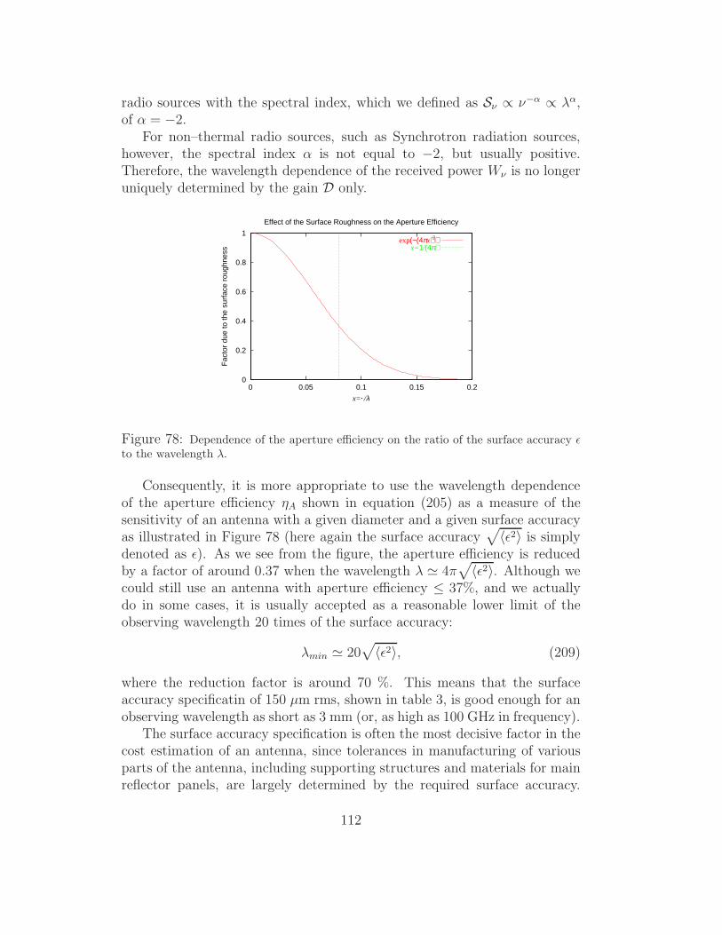
radio sources with the spectral index, which we defined as Sν ∝ ν−α ∝ λα,of α = −2.

For non–thermal radio sources, such as Synchrotron radiation sources,however, the spectral index α is not equal to −2, but usually positive.Therefore, the wavelength dependence of the received power Wν is no longeruniquely determined by the gain D only.

0

0.2

0.4

0.6

0.8

1

0 0.05 0.1 0.15 0.2

Fac

tor

due

to th

e su

rfac

e ro

ughn

ess

x=/λ

Effect of the Surface Roughness on the Aperture Efficiency

exp(−(4πx)2)x=1/(4π)

Figure 78: Dependence of the aperture efficiency on the ratio of the surface accuracy ǫto the wavelength λ.

Consequently, it is more appropriate to use the wavelength dependenceof the aperture efficiency ηA shown in equation (205) as a measure of thesensitivity of an antenna with a given diameter and a given surface accuracyas illustrated in Figure 78 (here again the surface accuracy

√

〈ǫ2〉 is simplydenoted as ǫ). As we see from the figure, the aperture efficiency is reducedby a factor of around 0.37 when the wavelength λ ≃ 4π

√

〈ǫ2〉. Although wecould still use an antenna with aperture efficiency ≤ 37%, and we actuallydo in some cases, it is usually accepted as a reasonable lower limit of theobserving wavelength 20 times of the surface accuracy:

λmin ≃ 20√

〈ǫ2〉, (209)

where the reduction factor is around 70 %. This means that the surfaceaccuracy specificatin of 150 µm rms, shown in table 3, is good enough for anobserving wavelength as short as 3 mm (or, as high as 100 GHz in frequency).

The surface accuracy specification is often the most decisive factor in thecost estimation of an antenna, since tolerances in manufacturing of variousparts of the antenna, including supporting structures and materials for mainreflector panels, are largely determined by the required surface accuracy.

112

ItemsFrequency in GHz

Remarks2.2 8.2 22.2 43.1

Illumination taper -2.39 -0.92 -1.30 -1.46

BlockingSubref. -0.16 -0.16 -0.16 -0.16

Stay -0.35 -0.35 -0.35 -0.35

spilloverMain ref. -0.27 -0.07 -0.01 -0.01

Subref. -0.97 -0.51 -0.18 -0.09

Surfaceaccuracy

Main ref. -0.01 -0.13 -0.94 -3.54 0.5mm rms

Subref. neg. -0.02 -0.15 -0.57 0.2mm rms

Setting neg. -0.04 -0.18 -0.66 Subref–feed

Horn cover loss -0.07 -0.06 -0.11 -0.24

Apertureefficiency

in dB -4.24 -2.26 -3.38 -7.08

in % 37.6% 59.4% 45.9% 19.6%

100 % gain in dB 47.2 58.6 67.3 73.1

Gain in dB 43.0 56.4 63.9 66.0

Feed & VSWR loss -2.0 (TBD) (TBD) (TBD)

Total gain in dB 41.0 (56.4) (63.9) (66.0)

Total efficiency in % 23.8% (59.4%) (45.9%) (19.6%)

Nominal gain in dB 40.7 56.1 63.6 65.7 at horn neck

Table 5: An example of the gain calculation for a 10 m diameter antenna. Numericalvalues are given in dB, unless otherwise stated. TBD stands for “to be determined”.

113

Therefore, the surface accuracy is carefully specified under certain environ-mental conditions, such as, ‘at night time, under wind speed less than 10m/s, and at elevation 45 degrees’. For high frequency radio telescopes, as-tronomers make regular efforts to improve the surface accuracy by preciselyadjusting surface panels.

An example of the gain calculation, taking into account the surface ac-curacy, as well as illumination taper, blocking, and spillover effects, is givenin table 5. One can easily confirm values of 100 % gain by equation (191),and values of surface accuracy effects for main reflector and subreflector byequation (205) (though we derived equation (205) for a main reflector, thesame discussion is applicable for a subreflector as well).

3.15 Pointing Accuracy

The main lobe axis of a radio telescope antenna may not be exactly orientedtowards a required direction due to the mechanical inaccuracy and the de-formations due to the gravity and the wind pressure. The angular offset

Main lobe axis

Required direction

ε

Gravity

Wind

Mechanical imaccuracy

θ

Figure 79: Pointing error.

ǫθ between the actual and required directions is called “pointing error” or“tracking error” (Figure 79). The rms value of the pointing error is oftencalled as “pointing accuracy” which we denote here as σθ

σθ =√

< ǫ2θ >. (210)

Let us consider the loss of the received power from a radio source due tothe pointing error. For simplicity, we assume a Gaussian power pattern P (θ)

114

with the peak power P0 and the HPBW Θ:

P (θ) = P0e−ln2( 2θ

Θ )2

(211)

0

0.2

0.4

0.6

0.8

1

-2 -1.5 -1 -0.5 0 0.5 1 1.5 2

Nor

mal

ized

pow

er p

atte

rn P

n(

)

x = /

Gaussian Beam with HPBW =

Figure 80: Gaussian beam.

If we assume that the main lobe axis is offset from the required directionin average by σθ, the received power from the radio source at the requireddirection is reduced in average by a factor of

P (σθ)

P0= e−4ln2(σθ

Θ )2

= e−2.7726( σθΘ )

2

. (212)

Figure 81 shows the power loss calculated by equation (212) as a function ofthe pointing accuracy σθ (which is denoted as σ in Figure 81 for simplicity).

It is evident from the figure that the pointing accuracy must be

σθ ≤1

10Θ (213)

to keep the power loss smaller than several %. Table 6 shows the pointing ac-curacy requirement given in equation (213) for some typical cases of antennadiameter D and observing wavelength λ on the basis of the approximateformula Θ ≃ λ/D.

Needless to say, a state–of–the–art technology of mechanical construction,good enough materials, and a sophisticated control system are needed, and

115

0

0.2

0.4

0.6

0.8

1

0 0.2 0.4 0.6 0.8 1 1.2 1.4

P(

)/Pmaxx = /

Power Loss due to the Pointing Error exp(−4ln2x2)

Figure 81: Power loss due to the pointing error.

D 10 m 20 m 22 m 21 m 45 m

νmax 43 GHz 43 GHz 43 GHz 150GHz 200 GHz

λmin 7 mm 7 mm 7 mm 2 mm 1.5 mm

HPBW ∼= λ/D 0.04 0.02 0.018 0.0055 0.0019

Required 0.004 0.002 0.0018 0.00055 0.00019

point. acc. (14”) (7.”2) (6.”6) (2.”0) (0.”7)

Table 6: Requirements to the pointing accuracy.

116

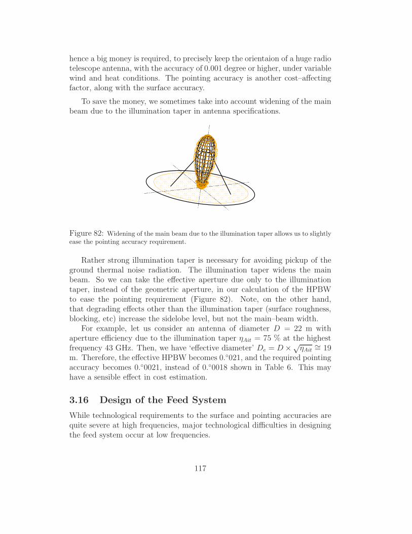
hence a big money is required, to precisely keep the orientaion of a huge radiotelescope antenna, with the accuracy of 0.001 degree or higher, under variablewind and heat conditions. The pointing accuracy is another cost–affectingfactor, along with the surface accuracy.

To save the money, we sometimes take into account widening of the mainbeam due to the illumination taper in antenna specifications.

Figure 82: Widening of the main beam due to the illumination taper allows us to slightlyease the pointing accuracy requirement.

Rather strong illumination taper is necessary for avoiding pickup of theground thermal noise radiation. The illumination taper widens the mainbeam. So we can take the effective aperture due only to the illuminationtaper, instead of the geometric aperture, in our calculation of the HPBWto ease the pointing requirement (Figure 82). Note, on the other hand,that degrading effects other than the illumination taper (surface roughness,blocking, etc) increase the sidelobe level, but not the main–beam width.

For example, let us consider an antenna of diameter D = 22 m withaperture efficiency due to the illumination taper ηAit = 75 % at the highestfrequency 43 GHz. Then, we have ‘effective diameter’ De = D×√

ηAit∼= 19

m. Therefore, the effective HPBW becomes 0.021, and the required pointingaccuracy becomes 0.0021, instead of 0.0018 shown in Table 6. This mayhave a sensible effect in cost estimation.

3.16 Design of the Feed System

While technological requirements to the surface and pointing accuracies arequite severe at high frequencies, major technological difficulties in designingthe feed system occur at low frequencies.

117

In order to efficiently receive or transmit radio signal with a Cassegrainparaboloidal antenna, beam of the feed horn shoud not be too wide com-pared with the subreflector, since otherwise we would suffer from a signifi-cant spillover of the signal beyond the edge of the subreflector. Thus, if wedenote the observing wavelength as λ, the diameter of the subreflector asDS, the diameter of the feed horn as DF , and the distance between the feedhorn and the subreflector as L (Figure 83), we have to require that the beam

DF

L

λDF

DS

Figure 83: Diameters of the feed horn DF and the subreflector DS and their mutualdistance L.

width of the feed horn is smaller than DS/L. The beam width is roughlygiven by λ/DF in the far–field. However the far–field approximation is def-initely inadequate in this case, since the subreflector is located in the nearfield (Fresnel region) of the feed horn, and therefore the beam is significantlybroader than the far–field one. Usually, a stringent condition:

10λ

DF<DS

L, (214)

is considered to be optimal.Suppose that we use a paraboloidal antenna at several observing wave-

lengths. Let the longest wavelength and corresponding feed diameter be λmax

and DF max, respectively. In order not to make either of the feed horn or thesubreflector too large, it is natural to select that DS ≃ DF max. Thus theequation (214) is reduced to

D2F max

λmaxL≥ 10. (215)

If we strictly adopt this condition, and assume L = 10 m for definiteness,we get following table of feed horn sizes for several cases of the longest wave-length. At observing frequencies as low as 1.4 GHz or 2 GHz, the optimum

118

λmax DF max

3 mm (100 GHz) 0.55 m

7 mm ( 43 GHz) 0.84 m

1.4 cm (22 GHz) 1.2 m

3.8 cm ( 8 GHz) 2.0 m

15 cm ( 2 GHz) 3.9 m

21 cm (1.4 GHz) 4.6 m

Table 7: Maximum observing wavelengths vs. diameters of the feed horns.

sizes of the feed horns are quite large. An example is shown in Figure 84.Sometimes, it is impractical to place big feed horns in receiver cabins.

Therefore, we are often forced to design smaller feed horns by adopting largersubreflectors, though this would cause larger blocking. Moreover, it is acommon practice to somewhat release the condition in equation (214) itself,partially sacrificing aperture efficiency at lower frequencies.

Huge S/X-band feed horn of Tsukuba 32 m

antenna is located here.

Figure 84: 2 and 8 GHz feed horn of Tsukuba 32 m antenna.

An alternative way to receive the low frequency radio waves without toomuch increasing the feed–horn and subreflector sizes is to use the primaryfocus (Figure 85). In the primary focus case, a feed horn must ‘illuminate’ thewhole area of a large main reflector. Therefore, a wide beam, and thereforea small diameter of the feed horn, is rather preferable.

119

Figure 85: A large feed horn and subreflector system (Left) or a primary feed system(Right) is needed for low frequency observations.

The large feed horns and subreflectors, or the feed and receiver blocks onthe primary focus, required for the low frequency observations, are nuisancesfor high frequency observations, since they may cause serious difficulties forachieving high aperture efficiency and pointing accuracy necessary at highfrequencies. Nevertheless, it is a natural desire of radio astronomers to ob-serve at as many frequency bands as possible, for example, from the 1.4 GHz

Figure 86: Initial Gregorian design of Nobeyama 45 m telescope, Japan (Left), adoptedfor receiving 1.4 GHz wave at primary focus, was later replaced by currently usedCassegrain design for better high–frequency performance (Middle). But still, a power-ful wave–beam–guide feed system and a big receiver room (Right) allow to receive widerange of frequency bands from 20 GHz to 230 GHz.

line of the neutral hydrogen to the 115 GHz CO line, say, with a single radiotelescope. Hence some sophisticated solutions are required (see examples inFigures 86, 87, and 88).

A very unique design of feed system is adopted in radiotelescope antennasof KVN (Korean VLBI Network), Korea, for simultaneous reception of 4observing bands at 22 GHz, 43 GHz, 86 GHz, and 129 GHz. Figure 89shows a preliminary design drawing of the multi–frequency–channel receivingsystem consisting of frequency selective surfaces and metal mirrors suitablyarranged to allow simultaneous feeding of the 4 frequency bands.

120

Figure 87: The tilted subreflector (Left) and feed horns arranged on a circle (Middle)in 25 m radio telescope of VLBA (Very Large Baseline Array), USA. Observing frequencybands from 1.4 GHz to 86 GHz can be easily changed by rotating the tilted subreflectoraround the symmetry axis of the main reflector as illustrated in a design drawing (Right).

Figure 88: Feed horns and receivers of 34 m VLBI antenna (Left) at Kashima, Japan,for various frequency bands are uplifted to the focus one by one, along rails inside the“Feed Cone” (Right).

121

Figure 89: A preliminary design of the multi–frequency–channel quasi–optics receivingsystem of KVN (Korean VLBI Network), Korea.

122

3.17 Visible Reference Point

As we saw earlier, it is desirable to make an antenna reference point (usually

Figure 90: In order to make the reference point visible from outside, one usually has toplace whole feed and receiver system in a small cabin in the back structure of the mainreflector (Left). For that purpose, we need compact feed systems. Examples of compactfeeds, 1.4 GHz/2.3 GHz feed horn used in Australian Telescope, and helical array S/Xfeed used in VERA, are shown in right two panels.

the cross point of Az and El axes) visible from outside, in order to tie thepoint to geodetic markers on the ground. This should be specially specified,when necessary, since otherwise antenna designers may place a receiver cabin,a wave–beam–guide system or something else around the cross point.

To keep the cross point in an empty space, we have to place the receivercabin somewhere else, most likely in a narrow space within the back structureunder the vertex of the main reflector (left panel of Figure 90). For thatpurpose, we have to design compact feed horns and receivers settable in thenarrow cabin (middle and right panels of Figure 90).

3.18 Alignment Errors and Offset of Axes

For both Alt–Azimuthal and Equatorial mount antennas, it is desirable thattwo axes (Az– and El–axes, or Right Ascension– and Declination–axes) ex-actly intersect at a point, and are mutually orthogonal. But after mechanicalconstruction of antennas, the two axes usually show some finite offsets andalignment errors (Figure 91). Tolerances to these quantities are often speci-fied to be less than a few mm and 0.01, respectively.

Even though such requirements are satisfied, they may be still largeenough to affect observational performances. The axes alignment erros mayaffect antenna pointings. The axes offset may require a correction in thehigh–precisioon geodetic VLBI analyses of an antenna position, since the off-set no longer permits us to select the reference point on an exact cross pointof the fixed and moving axes. Therefore, we must estimate and calibrate theaxes alignment errors, based on antenna pointing measurements. Also, we

123

Ideal vertical axisActual azimuth axis

Verticality error

Ideal axis

orthogonal to

Azimuth axis

Actual elevation

axis

Orthogonality

error

Az, El-axes offset

Figure 91: Images of Az axis verticality error, Az, El axes orthogonality error (Left),and Az, El axes offset (Right) in case of an Alt–Azimuth mount antenna.

have to estimate and calibrate the axes offset, based on local measurementsand/or geodetic VLBI measurements themselves.

3.19 Range of Motion

N EW

Celestial North

Pole

S

EW

N

(Az = 0 deg)

(Az = +270 deg)(Az = -270 deg)

Figure 92: Diurnal motion of a circumpolar radio source (Left) and required range ofazimuth motion (Right) for an Alt–Azimuth antenna.

For an Alt–Azimuth mount antenna, the range of azimuth and elevationangles must cover at least from −180 to +180 and from 0 ∼ 5 to 90,respectively, in order to be able to point toward any direction in the sky.However, we have to also take into account that a radio source may crossthe meridian line during an observation, from east to west, or west to east,in case of circumpolar sources, depending on their locations with respect to

124

the celestial pole. In order to smoothly track such diurnal motions of radiosources, the azimuth motion range is usually chosen from −270 to +270

with 0 selected at South (the same range corresponds to −90 – +450 inthe conventional azimuth angle measured eastward from North).

3.20 Slewing Speed

For VLBI antennas, especially for geodetic VLBI antennas, high slewingspeeds both in azimuth and elevation are preferable, since the high slewingspeeds allow us to effectively observe many sources on different points ofsky within a limited telescope time, without losing much time for antennarepointing from one source to another. Generally, slew speeds larger than2/sec in both axes are desirable.

An IVS (International VLBI Service for Geodesy and Astrometry) Work-ing Group Report “VLBI2010: Current and Future Requirements for Geode-tic VLBI Systems” (2005) proposes slewing speeds of 5/sec or higher inboth axes for future geodetic VLBI antennas. The high slew rate is neces-sary mainly for estimating and removing atmospheric and clock–offset effects,which are the largest error sources in current geodetic VLBI.

In recent VLBI observations, a technique called “fast switching” is oftenused. In this technique, orientation of a telescope is switched between twoclosely spaced radio sources (typically, separated by less than a few degrees)within a period of time as short as 20 to 60 seconds, for compensating irreg-ular atmospheric refraction effects (so called “phase–referencing”). For thefast switching, not only the slewing speeds, but also their accelerations mustbe sufficiently high, to realize the short switching cycle. For example, 3/secslewing speeds and 3/sec2 accelerations in both axes are recommended toachieve 20 second switching cycle for sources separated by 2 to 3 degrees.

3.21 Operational and Survival Loads

Operational and survival loads specify environmental conditions (tempera-ture, wind speed, seismic acceleration, etc.) under which antennas can beused for observations, and can survive in a stable stow position (usually El =90 and Az = 90 for an Az–El mount antenna) at rest, respectively. Theseloads must be determined depending on actual conditions of observing sites.

Usually, for mid–latitude stations with moderate wind, operational airtemperature condition from ∼ −20 to ∼ +40 C is appropriate.

As an example, we can distinguish following ranges of wind velocity v,though values listed are highly dependent on climatic conditions of observing

125

sites, especially whether they are in strong typhoon (cyclon, or hurricane)areas or not.

• Accuracy guaranteed range: (for example, 0 ms−1 ≤ v ≤ 10 ms−1).Suarface and pointing accuracies are guaranteed.

• Operational range: (for example, 0 ms−1 ≤ v ≤ 15 ms−1).We can conduct observations, though desired surface and pointing ac-curacies may not be met at high frequencies.

• Operable range: (for example, 15 ms−1 < v ≤ 30 ms−1).We must stop observations and move the antenna to “stow position”.

• Survival range: (for example, 30 ms−1 < v ≤ 70 ms−1).We must fix the antenna at the stow position with “stow pin”.

• Out of range: (for example, 70 ms−1 < v).In the worst case, the antenna could be destroyed.

For a strong typhoon area, the survival wind load limit should be 90 ms−1

or higher.

4 Antenna Temperature and Single Dish Imag-

ing

4.1 What Is the Antenna Temperature TA?

Pn(θ,φ)

θ=0

Iν(θ,φ)

TA

Figure 93: Antenna temperature.

“Antenna temperature”, usually denoted as TA, is an important, butagain a little confusing, quantity often used in radio astronomy, as well as

126

in VLBI geodesy. Actually, this is a quantity describing power Wν per unitfrequency bandwidth, centered at ν, received by an antenna. The poweris regarded as a “noise power added to a detector”, and converted to the“temperature of the noise” TA according to the Nyquist theorem: Wν =kTA. This is the antenna temperature.

Therefore, the amtenna temperature is a “temperature of a radio sourceas sensed by an antenna”, and has nothing common with the temperature ofthe antenna body, measurable by a thermometer.

If we denote the effective aperture of the antenna as Ae and the effectiveflux density of the source as Sν , then Wν is Wν = 1

2AeSν , in view of equation

(181). Therefore, the antenna temperature is given by

TA =1

2kAeSν . (216)

Then, denoting the normalized power pattern of the antenna as Pn(θ, φ)and the source intensity distribution as Iν(θ, φ) in the antenna–fixed coordi-nate system, we can transform the above equation to

Wν =1

2AeSν =

1

2Ae

∫∫

Ω

Pn(θ, φ) Iν(θ, φ) sin θ dθ dφ,

in view of equation (174). We can formally extend the above range of theintegration to the whole sky, since Pn(θ, φ) ≃ 0 outside the narrow beamanyway. Thus, using the solid angle element dΩ = sin θdθdφ, we express theantenna temperature in equation (216) as

TA =1

2kAe

∮

Pn(θ, φ) Iν(θ, φ) dΩ, (217)

(see Figure 93).Taking into account equation (184) which relates the effective aperture

Ae, the beam solid angle ΩA and the wavelength λ

AeΩA = λ2,

and the relation

ΩA =

∮

Pn(θ, φ)dΩ,

we can further transform equation (217) into

TA =λ2

2k

∮

Pn(θ, φ) Iν(θ, φ) dΩ∮

Pn(θ, φ)dΩ. (218)

127

If we express the intensity Iν through the brightness temperature TB:

Iν =2k

λ2TB,

we obtain

TA =

∮

Pn(θ, φ)TB(θ, φ) dΩ∮

Pn(θ, φ)dΩ. (219)

Therefore, the antenna temperature is the brightness temperature averagedover the antenna beam with the weighting function Pn(θ, φ), which is thenormalized power pattern.

4.2 Imaging with the Single Dish Radio Telescope

From the above discussions, we can interpret that the single dish radio tele-scope is a “huge power meter” measuring the weighted mean brightness tem-

1

2

34

5

6

7

89

10

11

1213

14

15

16

TA

Figure 94: Scanning observation for radio source imaging with a single dish radio tele-scope.

perature at a certain direction of the sky with the antenna power pattern asthe weight. The single dish radio telescope can draw the image of the radiosource by scanning from point to point meshed on the sky measuring thedistribution of the brightness (intensity) averaged over the beam. It is thusnaturally understood that the angular resolution of the image obtained by

128

the single dish radio telescope is determined by the beam size ∼ λ/D, whereλ is an observing wavelength and D is an antenna diameter (see Figure 94).

Let us examine three simplest cases of the source brightness distribution.

1. Point source Iν(s) = Sνδ(s − s0), where Sν is the source flux density,while s and s0 are unit vectors, and s0 is parallel to the beam axis. Inthis case we have

TA =1

2kAe

∮

Pn(s)Sν δ(s − s0) dΩ =1

2kAe Sν . (220)

We can measure the effective aperture Ae or the aperture efficiency ηA

by observing a point source of known flux density on the basis of thisequation.

2. Source of finite extent which slightly exceeds the main lobe:

TA = TB

∫

main lobe

Pn(θ, φ)dΩ

∮

Pn(θ, φ)dΩ=

ΩM

ΩATB = ηMTB. (221)

We can measure the main beam efficiency ηM by observing this kind ofsource with known brightness temperature (for example, a planet) onthe basis of the above equation.

Correct account of the main beam efficiency ηM is essential for properrecovery of the sky distribution of TB of the radio source in the singledish imaging. In most of VLBI observations, on the other hand, ηM

is not important since source sizes of VLBI objects are usually muchsmaller than the main lobe size.

3. Widely extended homogeneous source:

TA = TB. (222)

For example, we always receive the antenna temperature of 2.7 K fromthe cosmic microwave backgroud radiation.

Usually, the antenna temperature added by an astronomical radio sourceis very low, typically ranging from milli–Kelvins to Kelvins depending on thesource and the telescope. For example, if we receive a relatively strong radiosource with the effective flux density of 1 Jy ( = 10−26 W m−2 Hz−1) usingan 20 m diameter antenna with the aperture efficiency of 60 %, the antennatemperature is only about

TA =1

2kAeSν =

1

8kηAπD

2Sν ≃ 0.068 K.

129

This is of course much lower than the physical temperature of an antennabody which is always ≃ 300 K.

Q : Why can’t a radio telescope give us an image of the radio source just bya single observation like any optical telescope does?A : Unlike the photo plate or CCD plate, a radio telescope is usually equippedwith only one detecting element, the receiver. So what you can sense iswhether the received power is strong or weak in the beam direction. If youhave many receivers on the focal plane, then you will get the two–dimensionalimage at once. Now so–called multi–beam receiving systems are intensivelydeveloped at many radio astronomical observatories of the world for thatpurpose.

5 Receiving Systems

The very weak high frequency radio signal from an astronomical radio sourcecollected by the main reflector is amplified and frequency converted by thereceiving system and sent to the signal processing unit as the tractable signalof low frequency and with enough strength (Figure 95).

Local

Oscillator

Local

Oscillator

AmplifierMixer AmplifierMixer

Receiving system

Very weak

high-frequency

signal

Low Noise

Signal

Processing

Unit

tractable

signal

strong enough

and

low-frequency

Figure 95: A schematic view of a radio telescope receiving system.

On the other hand, the receiving system inevitably adds some noise tothe received signal, which may make it difficult to extract scientifically useful

130

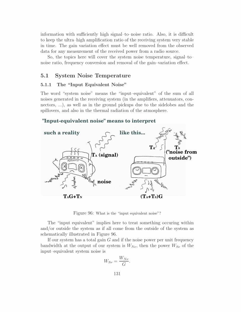
information with sufficiently high signal–to–noise ratio. Also, it is difficultto keep the ultra–high amplification ratio of the receiving system very stablein time. The gain variation effect must be well removed from the observeddata for any measurement of the received power from a radio source.

So, the topics here will cover the system noise temperature, signal–to–noise ratio, frequency conversion and removal of the gain–variation effect.

5.1 System Noise Temperature

5.1.1 The “Input Equivalent Noise”

The word “system noise” means the “input–equivalent” of the sum of allnoises generated in the receiving system (in the amplifiers, attenuators, con-nectors, ...), as well as in the ground pickups due to the sidelobes and thespillovers, and also in the thermal radiation of the atmosphere.

"Input-equivalent noise" means to interpret

such a reality like this...

TA (signal)

TS

("noise from outside")

TA

noise

TAG+TN (TA+TS)G

Figure 96: What is the “input equivalent noise”?

The “input equivalent” implies here to treat something occuring withinand/or outside the system as if all come from the outside of the system asschematically illustrated in Figure 96.

If our system has a total gain G and if the noise power per unit frequencybandwidth at the output of our system is WNν , then the power WSν of theinput–equivalent system noise is

WSν =WNν

G.

131

The “system noise temperature” TS is a temperature representing the powerWSν of the system noise in terms of the Nyquist theorem WSν = kTS, i.e.,

TS =WSν

k=WNν

kG.

5.1.2 Signal Attenuation and Thermal Noise

Let us consider how the thermal noise emerges within the receiving systemusing a model based on the radiative transfer equation, since it is likely thatthe absorption and emission of the radio wave occur in a similar way both inthe wave guide systems of the receivers and in the interstellar clouds.

Let us apply the radiative transfer equation:

dIνdl

= −κνIν + ǫν , (223)

to some “lossy piece” of our receiving system with temperature T (Figure97). For simplicity, we ignore the amplification for a while and consider theeffect of the attenuation only. In equation (223), Iν again stands for theintensity of the radio wave, l is the length along the optical path, and κν andǫν are the opacity (or absorption coefficient) and the emissivity, respectively.

A lossy piece in a receiving system

T

l

τν

signal

thermalnoise

0 l0

0τν(0)

.

Figure 97: Signal attenuation and thermal noise emission in a lossy piece of the receivingsystem.

Since it is likely that every element of the lossy piece, for example atten-uator, wave guide tube, connector, etc., is nearly in the thermodynamicaleqilibrium with each other, giving rise to the Boltzmann distribution among

132

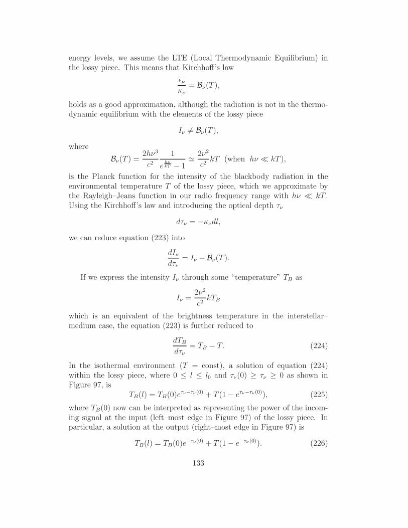
energy levels, we assume the LTE (Local Thermodynamic Equilibrium) inthe lossy piece. This means that Kirchhoff’s law

ǫνκν

= Bν(T ),

holds as a good approximation, although the radiation is not in the thermo-dynamic equilibrium with the elements of the lossy piece

Iν 6= Bν(T ),

where

Bν(T ) =2hν3

c21

ehνkT − 1

≃ 2ν2

c2kT (when hν ≪ kT ),

is the Planck function for the intensity of the blackbody radiation in theenvironmental temperature T of the lossy piece, which we approximate bythe Rayleigh–Jeans function in our radio frequency range with hν ≪ kT .Using the Kirchhoff’s law and introducing the optical depth τν

dτν = −κνdl,

we can reduce equation (223) into

dIνdτν

= Iν − Bν(T ).

If we express the intensity Iν through some “temperature” TB as

Iν =2ν2

c2kTB

which is an equivalent of the brightness temperature in the interstellar–medium case, the equation (223) is further reduced to

dTB

dτν= TB − T. (224)

In the isothermal environment (T = const), a solution of equation (224)within the lossy piece, where 0 ≤ l ≤ l0 and τν(0) ≥ τν ≥ 0 as shown inFigure 97, is

TB(l) = TB(0)eτν−τν(0) + T (1 − eτν−τν(0)), (225)

where TB(0) now can be interpreted as representing the power of the incom-ing signal at the input (left–most edge in Figure 97) of the lossy piece. Inparticular, a solution at the output (right–most edge in Figure 97) is

TB(l) = TB(0)e−τν(0) + T (1 − e−τν(0)). (226)

133

The first term in the RHS of equation (226) corresponds to the power of theinput signal attenuated by a factor of e−τν(0) in the lossy piece, while thesecond term shows the power of the newly added thermal noise.

Note that, if τν(0) = 0, the second term of the RHS of equation (226)is zero, so no thermal noise is added. Thus our general discussion, basedon a simple model, leads to an important conclusion that every receiverelement adds thermal noise as far as it attenuates the input signal.

Let us denote ε = e−τν(0) and call it “transmission efficiency”. ε = 1means perfect lossless transmission, and ε = 0 means complete attenuationor zero efficiency.

The thermal noise TN added in the system in temperature T with a trans-mission efficiency ε is TN = T (1− ε) according to equation (226). Therefore,the input–equivalent system noise temperature TS of such a system is bydefinition

TS =TN

ε=T (1 − ε)

ε. (227)

In order to get a low–noise device, one must achieve a high transmissionefficiency ε and/or cool the whole system in order to lower the environmentaltemperature T . This is the reason why modern highly sensitive radio tele-scope receivers are usually cooled to a very low temperature close to ∼ 15 Kor lower using cryogenic systems.

Q: Sometimes we see in advertisements of receivers for satellite broadcastingphrases like “65 K low noise amplifier in the room temperature”. Isn’t sucha statement against the principles of the thermodynamics?A: “65 K” here implies the system noise temperature which is the input–equivalent temperature of the noise added in the system. Since well madesystems could transmit signals with high efficiency (ε ≃ 1) even in the roomtemperature T ≃ 290K, there is no violation of the thermodynamics.

Q: If we slightly misalign a wave guide tube, the system noise temperature ofour receiving system could be as high as several thousand Kelvin. But whythe purely passive element like wave guide tube can increase the temperatureto such a high value?A: You could increase the input–equivalent noise temperature to an arbi-trarily high value if you only degrade the transmission efficiency. In fact, ifε = 0, then TN = T , but TS = ∞ !

134

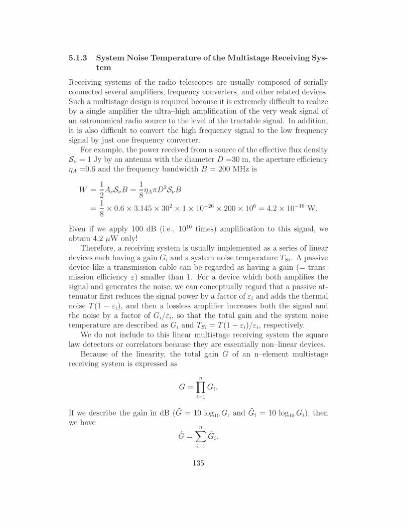
5.1.3 System Noise Temperature of the Multistage Receiving Sys-tem

Receiving systems of the radio telescopes are usually composed of seriallyconnected several amplifiers, frequency converters, and other related devices.Such a multistage design is required because it is extremely difficult to realizeby a single amplifier the ultra–high amplification of the very weak signal ofan astronomical radio source to the level of the tractable signal. In addition,it is also difficult to convert the high frequency signal to the low frequencysignal by just one frequency converter.

For example, the power received from a source of the effective flux densitySν = 1 Jy by an antenna with the diameter D =30 m, the aperture efficiencyηA =0.6 and the frequency bandwidth B = 200 MHz is

W =1

2AeSνB =

1

8ηAπD

2SνB

=1

8× 0.6 × 3.145 × 302 × 1 × 10−26 × 200 × 106 = 4.2 × 10−16 W.

Even if we apply 100 dB (i.e., 1010 times) amplification to this signal, weobtain 4.2 µW only!

Therefore, a receiving system is usually implemented as a series of lineardevices each having a gain Gi and a system noise temperature TSi. A passivedevice like a transmission cable can be regarded as having a gain (= trans-mission efficiency ε) smaller than 1. For a device which both amplifies thesignal and generates the noise, we can conceptually regard that a passive at-tenuator first reduces the signal power by a factor of εi and adds the thermalnoise T (1 − εi), and then a lossless amplifier increases both the signal andthe noise by a factor of Gi/εi, so that the total gain and the system noisetemperature are described as Gi and TSi = T (1 − εi)/εi, respectively.

We do not include to this linear multistage receiving system the squarelaw detectors or correlators because they are essentially non–linear devices.

Because of the linearity, the total gain G of an n–element multistagereceiving system is expressed as

G =n

∏

i=1

Gi.

If we describe the gain in dB (G = 10 log10G, and Gi = 10 log10 Gi), thenwe have

G =

n∑

i=1

Gi.

135

Now let us describe the output power Pi of i-th device in the n–elementmultistage receiving system through its gain Gi, system noise power kTSi,and input Pi−1, which is the output power of (i–1)–th device, as

Pi = (Pi−1 + kTSi)Gi, (228)

(see Figure 98).

Gi

kTsi

Pi-1 Pi = (Pi-1 + kTsi) Gi

Input power Output power

Figure 98: Input and output of a linear device with gain Gi and system noise temperatureTSi.

Then if we denote the input power to the first device as P0 = kTA, whereTA is the antenna temperature due to an astronomical source, the outputpower of n–th device is expressed as

Pn = · · ·[(P0 + kTS1)G1 + kTS2]G2 + kTS3G3 + · · · + kTSnGn

= kTA

n∏

i=1

Gi + kTS1

n∏

i=1

Gi + kTS2

n∏

i=2

Gi + kTS3

n∏

i=3

Gi

+ · · · + kTSnGn, (229)

(Figure 99).

TA

Ts1 Ts2 Ts3 Ts4 Tsn

Input Output

G1 G2 G3 G4 Gn

Figure 99: Multistage receiving system.

Denoting the total gain of the system as G =n∏

i=1

Gi and equating Pn in

equation (229) to the sum of the input power and the sytem noise powermultiplied by the total gain

Pn = k(TA + TS)G, (230)

136

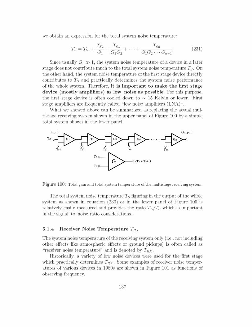
we obtain an expression for the total system noise temperature:

TS = TS1 +TS2

G1+

TS3

G1G2+ · · · + TSn

G1G2 · · ·Gn−1. (231)

Since usually Gi ≫ 1, the system noise temperature of a device in a laterstage does not contribute much to the total system noise temperature TS. Onthe other hand, the system noise temperature of the first stage device directlycontributes to TS and practically determines the system noise performanceof the whole system. Therefore, it is important to make the first stagedevice (mostly amplifiers) as low–noise as possible. For this purpose,the first stage device is often cooled down to ∼ 15 Kelvin or lower. Firststage amplifiers are frequently called “low noise amplifiers (LNA)”.

What we showed above can be summarized as replacing the actual mul-tistage receiving system shown in the upper panel of Figure 100 by a simpletotal system shown in the lower panel.

TA

Ts1 Ts2 Ts3 Ts4 Tsn

Input Output

G1 G2 G3 G4 Gn

TA

TS

(TA + TS) GG

Figure 100: Total gain and total system temperature of the multistage receiving system.

The total system noise temperature TS figuring in the output of the wholesystem as shown in equation (230) or in the lower panel of Figure 100 isrelatively easily measured and provides the ratio TA/TS which is importantin the signal–to–noise ratio considerations.

5.1.4 Receiver Noise Temperature TRX

The system noise temperature of the receiving system only (i.e., not includingother effects like atmospheric effects or ground pickups) is often called as“receiver noise temperature” and is denoted by TRX .

Historically, a variety of low noise devices were used for the first stagewhich practically determines TRX . Some examples of receiver noise temper-atures of various devices in 1980s are shown in Figure 101 as functions ofobserving frequency.

137

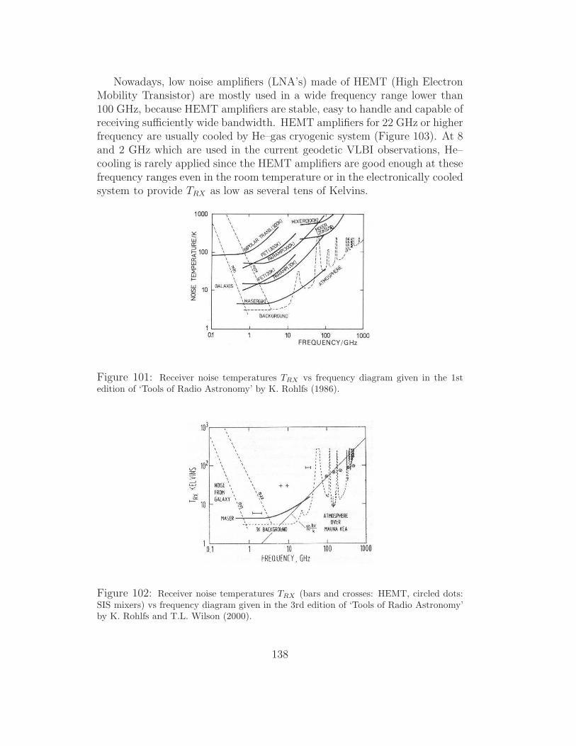
Nowadays, low noise amplifiers (LNA’s) made of HEMT (High ElectronMobility Transistor) are mostly used in a wide frequency range lower than100 GHz, because HEMT amplifiers are stable, easy to handle and capable ofreceiving sufficiently wide bandwidth. HEMT amplifiers for 22 GHz or higherfrequency are usually cooled by He–gas cryogenic system (Figure 103). At 8and 2 GHz which are used in the current geodetic VLBI observations, He–cooling is rarely applied since the HEMT amplifiers are good enough at thesefrequency ranges even in the room temperature or in the electronically cooledsystem to provide TRX as low as several tens of Kelvins.

Figure 101: Receiver noise temperatures TRX vs frequency diagram given in the 1stedition of ‘Tools of Radio Astronomy’ by K. Rohlfs (1986).

Figure 102: Receiver noise temperatures TRX (bars and crosses: HEMT, circled dots:SIS mixers) vs frequency diagram given in the 3rd edition of ‘Tools of Radio Astronomy’by K. Rohlfs and T.L. Wilson (2000).

138

At frequency higher than 100 GHz, He–cooled SIS (superconductor–insulator–superconductor) mixers instead of the amplifiers are usually used as the firststage device, since it is still difficult to make reliable low noise amplifiers forthe high frequency range (Figure 104).

Figure 102 shows performance of the HEMT amplifiers and SIS mixersin 2000s. Note that many devices shown in Figure 101, including old FETand Parametric amplifiers, are no longer shown in Figure 102, because theyare mostly replaced by HEMT amplifiers.

Figure 103: He–cooled 22 GHz and 43 GHz HEMT amplifiers placed in common cryo-genic dewers and mounted on VERA dual–beam receiving system.

Figure 104: He–cooled SIS–mixer in the 100 GHz and 150 GHz dual channel receiversystem of Taedok Radio Astronomy Observatory, Korea.

139

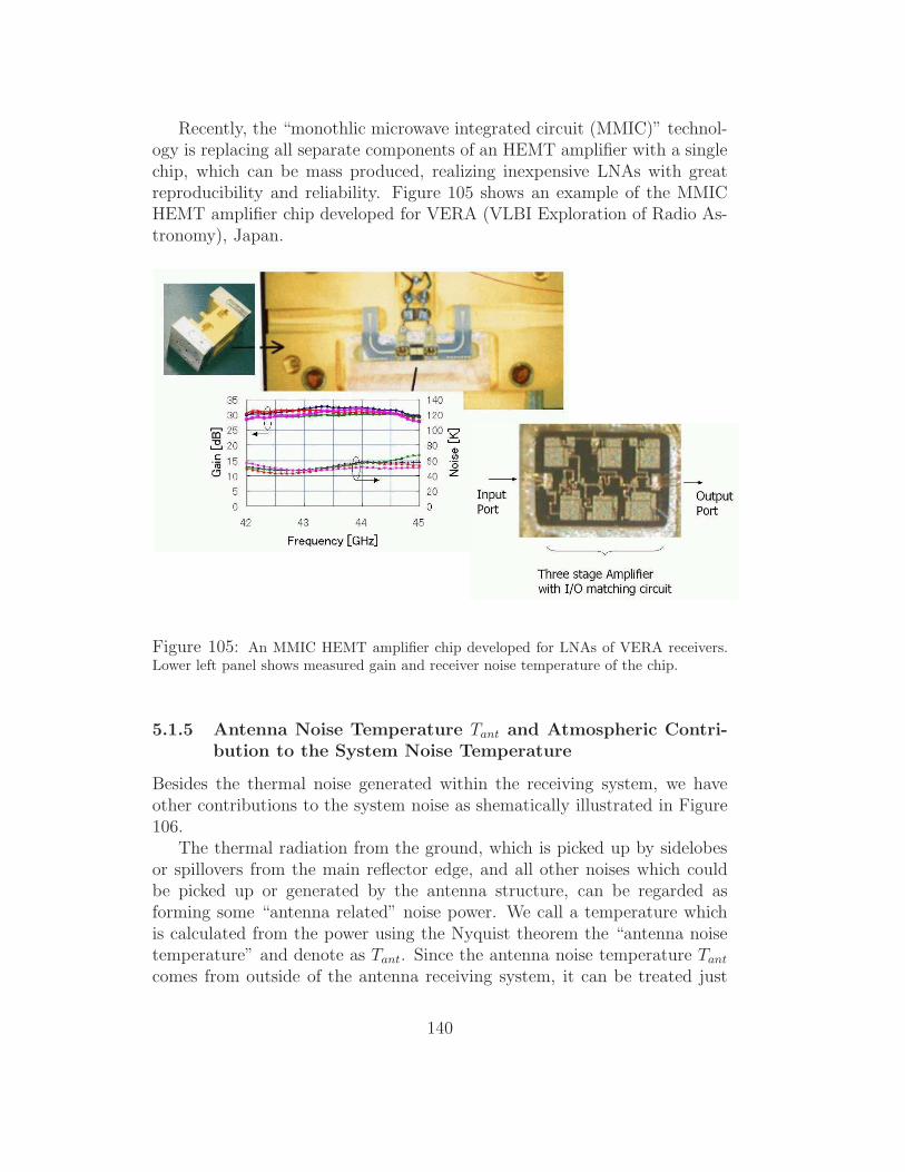
Recently, the “monothlic microwave integrated circuit (MMIC)” technol-ogy is replacing all separate components of an HEMT amplifier with a singlechip, which can be mass produced, realizing inexpensive LNAs with greatreproducibility and reliability. Figure 105 shows an example of the MMICHEMT amplifier chip developed for VERA (VLBI Exploration of Radio As-tronomy), Japan.

Figure 105: An MMIC HEMT amplifier chip developed for LNAs of VERA receivers.Lower left panel shows measured gain and receiver noise temperature of the chip.

5.1.5 Antenna Noise Temperature Tant and Atmospheric Contri-bution to the System Noise Temperature

Besides the thermal noise generated within the receiving system, we haveother contributions to the system noise as shematically illustrated in Figure106.

The thermal radiation from the ground, which is picked up by sidelobesor spillovers from the main reflector edge, and all other noises which couldbe picked up or generated by the antenna structure, can be regarded asforming some “antenna related” noise power. We call a temperature whichis calculated from the power using the Nyquist theorem the “antenna noisetemperature” and denote as Tant. Since the antenna noise temperature Tant

comes from outside of the antenna receiving system, it can be treated just

140

300 K

side lobe pick upspill over

main lobeatmospheric noise

Figure 106: Atmospheric and ground pickup contributions to the system noise temper-ature.

as an input noise to the first stage of the receiving system. This means thatTant can be simply added to TS1 in the RHS of equation (231). Of course,the antenna noise temperature must strongly depend on the elevation of theantenna beam since the ground pickup must be stronger at lower elevations.

The noise temperature TNair due to the thermal radiation of the atmo-sphere of temperature Tatm also contributes to the system noise temperature.The noise generation and signal attenuation in the atmosphere are describedby the radiative transfer theory, which we discussed in Chapter 1 and usedin subsection 5.1.2 for modeling the noise generation in a lossy piece of thereceiving system.

Specifically, the radiative transfer equation under the assumption of thelocal thermodynamic equilibrium is given by equation (224):

dTB

dτν= TB − Tatm,

where TB is the brightness temperature and τν is the optical depth at anobserving frequency ν. If we assume the isothermal atmosphere (i.e. Tatm =const, which is not a very bad approximation in lower layers of the atmo-sphere where the signal attenuation is significant), solution of the aboveequation at the bottom of the atmosphere is given by equation (226):

TB = T ⋆Be

−τatm + Tatm(1 − e−τatm),

where T ⋆B is the brightness temperature of a radio source outside of the at-

mosphere and τatm is the total optical depth at frequency ν due to the wholeatmosphere. Note that first and second terms in the RHS of this equation

141

represent contributions from the extra–atmospheric radio source and the at-mospheric thermal noise, respectively.

Now we calculate the “temperature sensed by an antenna” directed to-wards a radio source as a weighted average of TB over the antenna beamusing equation (219):

∮

Pn(θ, φ)TB(θ, φ) dΩ∮

Pn(θ, φ)dΩ=

∮

Pn(θ, φ)T ⋆B(θ, φ) dΩ

∮

Pn(θ, φ)dΩe−τatm + Tatm(1 − e−τatm),

where θ and φ are angular coordinates in the antenna–fixed coordinate systemas before, Pn(θ, φ) is the normalized power pattern, and τatm here is the totalotical depth along the direction of the antenna beam. When we derived theabove equation, we assumed that Tatm and τatm are almost constant withinthe narrow solid angle of the antenna beam. The first term in the RHSis the antenna temperature due to the attenuated signal from the extra–atmospheric radio source:

TA =

∮

Pn(θ, φ)T ⋆B(θ, φ) dΩ

∮

Pn(θ, φ)dΩe−τatm ,

and the second term is the thermal noise generated in the atmosphere:

TNair = Tatm(1 − e−τatm). (232)

Note that τatm and therefore TNair vary significantly with elevation of theantenna beam.

Since both TA and TNair are inputs of the antenna from outside, theatmospheric noise temperature TNair is just added to TS1 in the RHS ofequation (231) when we calculate the total system noise temperature.

Therefore, the total system noise temperature TS, including the receivernoise, the antenna noise and the atmospheric noise effects, is given by

TS = TRX + Tant + Tatm(1 − e−τatm). (233)

Equation (233) is usually given as a general expression of the system noisetemperature.

However, when a radio telescope is covered by a radome or a feed–conecover (see Figure 88 as an example) which slightly emits thermal noise ra-diation, or is exposed to a strong human made radio frequency interference(RFI), one should take into acount contributions of these additional noisesources to the system noise temperature.

When we consider the contribution of the radome or feed–cone cover tothe system noise temperature, in particular, we have to distinguish reflection

142

loss and absorption loss due to the cover. Reflection on the cover materialand supporting frames blocks a part of incident rays and therefore reducessignal power to be received, but does not generate noise radiation. On theother hand, absorption induces both signal attenuation and noise generation.Consequently, only the absorption loss contributes to the system noise.

If we denote the absorption loss of the radome or feed–cone cover as1 − e−τmem , where τmem is the optical depth of the cover membrane at theobserving frequency, and if we assume that temperature of the membraneis just equal to the air temperature Tatm, then both signal and atmosphericnoise are attenuated by e−τmem and, at the same time, new thermal noiseTatm(1 − e−τmem) is generated in the membrane. Therefore, we have

TA =

∮

Pn(θ, φ)T ⋆B(θ, φ) dΩ

∮

Pn(θ, φ)dΩe−(τatm+τmem),

andTS = TRX + T ′

ant + Tatm[1 − e−(τatm+τmem)],

for the antenna temperature TA and the system noise temperature TS whenthe radome or feed–cone cover effect is significant. Here we denoted theantenna noise temperature as T ′

ant taking into account that a part of theground pickup radiation must be attenuated by the cover membrane.

5.2 Frequency Conversion

If a radio signal is band limited, that means it has non–zero spectral powerwithin a certain frequency range with a finite bandwidth only, we can shiftthe central frequency of such a signal (usually to the lower side) withoutlosing any spectral information (Figure 107). This is the principle of thefrequency conversion, which can be generally interpreted as a result of theshift theorem of Fourier transformation.

ν0

spectrum

Figure 107: Frequency shift of the band limited signal.

Frequency conversion is needed in the radio telescope receiving systembecause

143

1. the received signal is much less attenuated in transmission cables and ismuch easily filtered, detected by a square–law detector, digitized, andso on, in the low frequency (lower than 1 GHz, say) than in the highfrequency, and

2. it is necessary that the input and output signals are in different fre-quency bands before and after the enormous amplification of severaltens to hundreds dB for avoiding possible leakage of a small amountof output power back to the input which could terribly oscillate thesystem.

5.2.1 Technical Terms in the Frequency Conversion

mixer

BPF

LO

νLORF

νIF

ν - νLO

frequency standard

Down converter

tt

Figure 108: Elements and technical terms used in the frequency conversion.

A little peculiar technical terms are used in descriptions of the frequencyconversion. They are

144

• radio frequency (RF): the high frequency involved in the band whichis directly received by an antenna, sometimes called also as “sky fre-quency”,

• intermediate frequency (IF): the low frequency obtained by thefrequency conversion,

• local oscillator (LO): an oscillator which provides a sinusoidal refer-ence signal with a specified frequency,

• mixer: a nonlinear device which multiplies the reference signal to thereceived signal,

• bandpass filter (BPF): a filter which passes only necessary band ofthe intermediate frequency and cuts off all other frequency componentsin the output from the mixer,

• down converter: a unit composed of the LO, mixer and BPF whichconverts RF ν to IF ν−νLO, where νLO is the frequency of the referencesignal provided by the LO which is often called “LO frequency”,

• superheterodyne receiver: a receiver based on the frequency con-version technique.

Figure 108 shows elements of the frequency conversion. For example, ina typical Mark III–type geodetic VLBI observation at 8 GHz, we can choose8180 MHz ∼ 8600 MHz as the RF band and 8080 MHz as the LO frequencyνLO to get 100 MHz ∼ 520 MHz as the IF band.

5.2.2 What Is the Mixer?

The main part of the mixer is a device (for example, a mixer diode) whichhas a nonlinear current (I) — voltage (V ) relation:

I = a0 + a1V + a2V2 + a3V

3 + · · ·, (234)

where ai’s are constant coefficients.The received signal and the reference signal from LO are first summed

up before entering to the nonlinear device. So, denoting the voltage of afrequency component with the angular frequency ω = 2πν in the RF bandas Vs cos(ωt + φ) and the voltage of the reference signal with LO angularfrequency ωLO as VLO cos(ωLOt + φLO), where φ and φLO are initial phases,we have the summed input voltage V to the nonlinear device:

V = Vs cos(ωt+ φ) + VLO cos(ωLOt+ φLO). (235)

145

nonlineardevice

mixer

RF

LO

IF

Down converter

BPF

Figure 109: General concept of the mixer.

Therefore, we obtain a term proportional to VsVLO in the output current fromthe nonlinear device due to the second order term a2V

2 of the I–V relationin equation (234), which is

a2VsVLO cos(ωt+ φ) cos(ωLOt+ φLO)

=1

2a2VsVLO cos[(ω + ωLO)t+ φ+ φLO]

+1

2a2VsVLO cos[(ω − ωLO)t+ φ− φLO]. (236)

The first and second terms in the RHS of equation (236) correspond to up–converted and down–converted frequencies, respectively. So, we can realizethe desired frequency conversion by picking up only the down–convertedfrequency with a suitably designed BPF which passes the down–convertedfrequency and cuts off the up–converted as well as all other frequencies pro-duced by the I–V relation in equation (234). Note that the linearity of thereceived signal is preserved in this procedure though we used the nonlineardevice.

5.2.3 Upper Sideband (USB) and Lower Sideband (LSB)

If the LO frequency is chosen within the received RF band, two frequenciesωU and ωL satisfying relations

ωU − ωLO = ωIF (237)

andωLO − ωL = ωIF , (238)

146

ω0ω

LOω0ω

LO+0

IF RF

LSB USB

ω0

ωLO

-

Figure 110: Upper and lower sidebands are converted to the same IF band.

both pass through the BPF and have the same IF ωIF . In fact, they bothhave the same cos(ωIF t+ · · ·) form in the mixer output as the above discusionon the mixer principle shows. The frequency higher than the LO frequencyforms “upper sideband (USB)” and the lower one forms “lower sideband(LSB)”. When the both sidebands contribute to the IF band, the IF spectrumturns out to be a superposition of the down–converted spectra of the USBand the frequency–inverted LSB as illustrated in Figure 110. Frequencies indifferent sidebands corresponding to the same IF frequency are called “mirrorfrequencies” or “image frequencies”.

5.2.4 Sideband Rejection

ω0ω

LOω0ω

LO+0

IF RF

LSB USB

IF BPF RF BPF

RF BPF IF BPF

LO

mixerRF IF

ω0ωLO

-

Figure 111: Sideband rejection in terms of the BPF in the RF band.

A superheterodyne receiving system which accepts both USB and LSBcontributions to the IF band is called “double sideband (DSB)” receiver,while a system which receives only one of the two sidebands is called “singlesideband (SSB)” receiver.

147

local oscillator

mixer IF amppre-amp

Tape recorder

ν0

RF IF ν ν - ν0

analog digital

instrumental delay

correlator

correlator

radio

wave current or voltage power display

Single dish telescope

Connected Interferometer

VLBI

Tape playback

unit (PBU)

SQ integrator

multiplier integrator

SQ-law detector

multiplier integrator

Figure 112: Superheterodyne receiving systems in single dish telescope (Top), connectedinterferometer (Middle) and VLBI (Bottom).

148

For observations of continuum sources, the DSB receivers offer bettersensitivity, while for observations of spectralline sources, SSB receivers arepreferred. In VLBI observations, SSB receivers are mostly used even forcontinuum sources for avoiding complication of the data processing.

The process to remove unnecessary sideband for a SSB observation iscalled “sideband rejection” or “image rejection”. The rejection is most simplyrealized by a suitable BPF in the RF range which limits the RF band of themixer input in such a way that the LO frequency falls outside of the inputband (Figure 111).

The frequency–conversion or superheterodyne technology is generally usedin all kinds of radio telescopes including single dish telescopes, connected el-ement interferometers and VLBIs (Figure 112).

5.3 Signal–to–Noise Ratio of a Single–Dish Radio Tele-scope

How can we estimate sensitivity (or signal–to–noise ratio) of a single–dishradio telescope?

In order to answer to this question, we have to address following threeproblems beforehand:

1. how can we separate a source signal and a system noise in our single–dish observation when both of them are Gaussian random noises?

2. how can we detect a weak source signal out of an overwhelmingly strongsystem noise?

3. how do we define the signal–to–noise ratio for a single–dish radio tele-scope?

We will consider these problems one by one.

1. How can we separate a signal and a noise?

In order to detect a signal of a radio source, of course we have to separatethe signal from all kinds of noises coming from the receiver system and theenvironment (the system noise). However, the radio source signal itself is aGaussian random noise, which is much the same with the system noise. Inother words, we cannot separate the radio–source signal and the system noiseby their temporal behaviors. If the observed source is a spectralline source,we could in principle distinguish the source signal by its spectral shape. Butin case of a continuum source, spectral shapes of the signal and the systemnoise are much the same again. So there is no way for signal detection for acontinuum source other than just watching an increase and a decrease of the

149

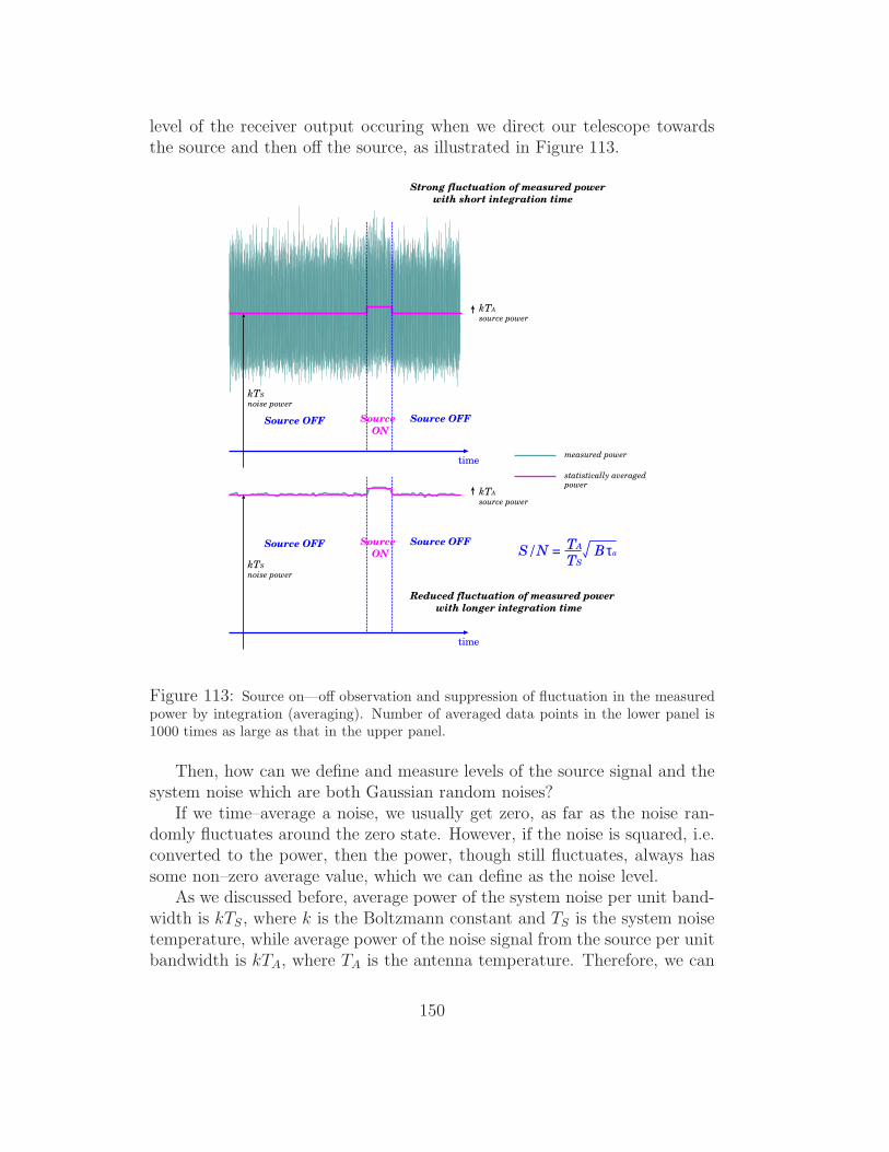
level of the receiver output occuring when we direct our telescope towardsthe source and then off the source, as illustrated in Figure 113.

kTS

noise power

Strong fluctuation of measured power

with short integration time

S/N = B τaTA

TS

time

kTS

noise power

kTA

source power

Reduced fluctuation of measured power

with longer integration time

time

kTA

source power

measured power

statistically averagedpower

Source

ON

Source OFFSource OFF

Source

ON

Source OFFSource OFF

Figure 113: Source on—off observation and suppression of fluctuation in the measuredpower by integration (averaging). Number of averaged data points in the lower panel is1000 times as large as that in the upper panel.

Then, how can we define and measure levels of the source signal and thesystem noise which are both Gaussian random noises?

If we time–average a noise, we usually get zero, as far as the noise ran-domly fluctuates around the zero state. However, if the noise is squared, i.e.converted to the power, then the power, though still fluctuates, always hassome non–zero average value, which we can define as the noise level.

As we discussed before, average power of the system noise per unit band-width is kTS, where k is the Boltzmann constant and TS is the system noisetemperature, while average power of the noise signal from the source per unitbandwidth is kTA, where TA is the antenna temperature. Therefore, we can

150

expect an increase in the power of the receiver output due to TA over thenoise power due to TS, when our telescope catches a source. Thus we can, inprinciple, separate the signal from the noise in this way.

2. How can we detect a weak signal out of a much stronger noise?

However, the signal TA is usually much (several thousand times, say)smaller than the very high “noise floor” TS for most of astronomical radiosources. Moreover, the squared random noise, i.e. the instantaneous noisepower, itself randomly fluctuates in time around its average value, as we saidbefore. If the fluctuation is larger than the average signal power, it is quitehard to detect the small increase of the output power due to the signal.

Fortunately, however, we can suppress the fluctuaion if we time–averagethe output power during some period of time (or “integrate” it). While theintegration is not sufficiently long, it is still difficult to detect a weak sourcesignal as illustrated in the upper panel of Figure 113. But if the integrationtime is long enough, the fluctuation is well suppressed and we can firmlydetect the source as shown in the lower panel of Figure 113.

Actually, what we measure by our radio telescope is an integrated receivedpower. In fact, as we saw in Figure 112, the radio signal from an astronomicalsource received by a radio telescope antenna is transmitted, together with thesystem noise, through the receiving system as a voltage (or a current). Afterseveral steps of amplification and down–conversion, a unit like a square–law detector squares the voltage to make the power, which is then time–averaged for some integration time by an integrator, and eventually displayedto observers by a power meter or other devices.

Note that the integration (time–averaging) is not a specific feature of thesource on–off observation of a continuum source only, but is common to allkinds of radio astronomical observations. For example, source spectra whichwe obtain for spectralline sources are actually time–averaged power spectraof received voltages. If the integration is insufficient, we get jaggy and time–fluctuating spectrum due mainly to the noise, from which we cannot deriveany reliable source spectrum.

Thus, we can detect a weak signal out of a much stronger noise if weintegrate the received power for a sufficiently long time.

3. How do we define the signal–to–noise ratio?

Now it is natural to define the signal–to–noise ratio in the single–dishradio astronomy as a quantity showing how well we can detect the sourcethrough the integration (time–averaging) of the received power.

Specifically, we define it as a ratio between the average signal power andthe level of fluctuation (standard deviation) of the time–averaged noisepower.

151

Do not mix up this with the original ratio of the average signal powerand the average noise power TA/TS, which is hopelessly small for most ofastronomical radio sources.

This is our answer to the third problem.

A statistical theory of the dispersion of the time–averaged squared ran-dom data, which we will discuss in Chapter 3 in detail, shows that the signal–to–noise ratio S/N of the integrated received power is expressed in terms ofthe antenna temperature TA, system noise temperature TS, bandwidth Band integration (or averaging) time τa by a formula:

S/N =TA

TS

√

Bτa. (239)

Or, if we express TA, following equation (216), through Boltzmann constantk = 1.381 × 10−23, effective aperture Ae, effective flux density Sν , diameterD and aperture efficiency ηA of a circular aperture antenna, we have

S/N =AeSν

2kTS

√

Bτa =πηAD

2Sν

8kTS

√

Bτa. (240)

Thus, we can estimate the signal–to–noise ratio in a single–dish observationon the basis of this equation.

As we mentioned earlier, even if we observe a relatively strong radiosource with the effective flux density of 1 Jy ( = 10−26 W m−2 Hz−1) usingan 20 m diameter antenna with the aperture efficiency of 60 %, the antennatemperature is only about

TA =1

2kAeSν =

1

8kηAπD

2Sν ≃ 0.068 K.

Therefore, if the system noise temperature is 100 K (which is not a bad figure,by the way), the original ratio of the average signal power and the averagesystem noise power is only

TA

TS= 6.8 × 10−4 !

Nevertheless, if we observe the source with a fairly wide frequency bandwidthB = 100 MHz and integrate the output power for 1 second, then the signal–to–noise ratio is

S/N =TA

TS

√

Bτa = 6.8,

and therefore well detectable! This is the way how radio astronomers receivethe radio source signals.

152

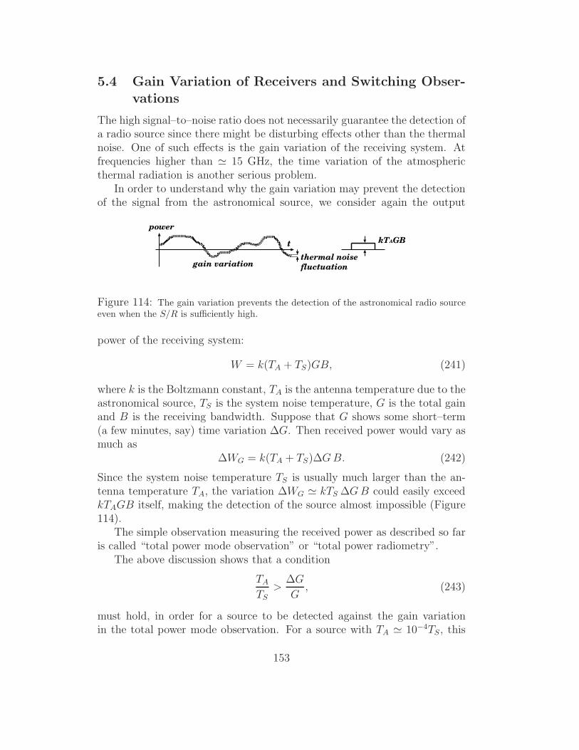
5.4 Gain Variation of Receivers and Switching Obser-vations

The high signal–to–noise ratio does not necessarily guarantee the detection ofa radio source since there might be disturbing effects other than the thermalnoise. One of such effects is the gain variation of the receiving system. Atfrequencies higher than ≃ 15 GHz, the time variation of the atmosphericthermal radiation is another serious problem.

In order to understand why the gain variation may prevent the detectionof the signal from the astronomical source, we consider again the output

t

thermal noise

fluctuation

kTAGB

power

gain variation

Figure 114: The gain variation prevents the detection of the astronomical radio sourceeven when the S/R is sufficiently high.

power of the receiving system:

W = k(TA + TS)GB, (241)

where k is the Boltzmann constant, TA is the antenna temperature due to theastronomical source, TS is the system noise temperature, G is the total gainand B is the receiving bandwidth. Suppose that G shows some short–term(a few minutes, say) time variation ∆G. Then received power would vary asmuch as

∆WG = k(TA + TS)∆GB. (242)

Since the system noise temperature TS is usually much larger than the an-tenna temperature TA, the variation ∆WG ≃ kTS ∆GB could easily exceedkTAGB itself, making the detection of the source almost impossible (Figure114).

The simple observation measuring the received power as described so faris called “total power mode observation” or “total power radiometry”.

The above discussion shows that a condition

TA

TS>

∆G

G, (243)

must hold, in order for a source to be detected against the gain variationin the total power mode observation. For a source with TA ≃ 10−4TS, this

153

implies that we must suppress the gain variation of the receiving system∆G/G within a level as small as

∆G

G< 10−4, (244)

which is practically quite difficult.Therefore, radio astronomers apply switching techniques to the single dish

telescope observations in order to avoid the gain variation effect and firmlydetect the weak astronomical radio sources.

5.4.1 Dicke Mode Switching Observation

A switching method was proposed by R.H. Dicke in 1946 and has been widelyused. In this method, two input signals (voltages), one from the antenna feedhorn and another from a noise source (for example, a cooled resistor) of aconstant temperature TR are quickly switched in front of the receiving systemand, at the same time, the sign of the output power from the square–lawdetector is reversed with the same switching timing which are then summedup (i.e., the powers from the two inputs are subtracted) and averaged asshown in Figure 115.

SQ detector Σx (+1)

x (-1)

switch-timing control pulsenoise source

outputTA

TR

Figure 115: A general scheme of the Dicke mode receiver.

The square–law detector yields a power

WA = k(TA + TS)GB, (245)

in the upper switch position in Figure 115, while in the lower switch position,

WR = k(TR + TRX)GB, (246)

154

where TRX is the receiver noise temperature. At relatively low observingfrequency ≤ 15 GHz, the atmospheric contribution to the system noise tem-perature is much smaller than TRX , and the ground pickup effects are smallas far as the elevation is not very low. Consequently, TS

∼= TRX in equa-tion (233) for the low frequency and moderately high elevation observations.Therefore, the difference output from the Dicke mode receiver gives us

WA −WR∼= k(TA − TR)GB, (247)

provided that the switching interval is short enough compared with the timescale of the gain variation. Therefore, the effect of the gain variation to thisdifference output is

∆(WA −WR) ∼= k(TA − TR) ∆GB (248)

and hence the condition for the source detection is now

TA

TA − TR>

∆G

G(249)

instead of equation (243). This new condition is easily satisfied if we suitablychoose the temperature of the noise source TR low enough to be TR ∼ TA.

Instead of the noise source, we could use a small antenna like a hornantenna looking at the sky for the switching observation (Figure 116).

SQ detector Σx (+1)

x (-1)

switch-timing control pulse

outputTA

Tsky

Figure 116: A switching mode observation using a small antenna.

For spectralline sources, quick “frequency switching” between inside andoutside of the spectral lines can be used for detecting the sources against thegain variation of the receiving system.

155

5.4.2 Beam Switch

At frequencies higher than ≃ 15 GHz, the radio signal from an astronomicalradio source is badly masked by the time variation of the thermal radiation ofthe atmosphere along with the gain variation of the receiving sysytem. Also,it is not desirable at the high frequencies to install the switching mechanismin the RF signal transmision system since the switches themselves couldbecome additional noise sources.

In this circumstance, another technique called “beam switching” is effec-tive. The beam switching is a quick switching of the antenna beam betweenthe on–source and the off–source directions and measuring the difference ofthe received powers at the two directions (Figure 117).

Σx (+1)

x (-1)

output

switch-timing control pulse

TA

Tsky

Figure 117: Beam switching between the on–source and the off–source directions.

Since the on–source output power is

Wsource = k(TA + TS)GB, (250)

while the off–source output power is

Wsky = kTSGB, (251)

the power difference yields

Wsource −Wsky = kTAGB. (252)

If gain varies by ∆G, we have ∆(Wsource −Wsky) = kTA∆GB. Therefore,we can easily detect kTAGB as far as ∆G≪ G.

156

Also, we can obtain the antenna temperature TA by a simple formula

TA =Wsource −Wsky

Wsky

TS, (253)

if we know the system noise temperature TS.The atmospheric thermal radiation effects are well cancelled out in the

above procedure, as far as the two beam directions are not too much sepa-rated on the sky.

sub reflector

rotating mirror

feed horn

rotationaxis

Figure 118: Beam switching using the vaned–wheel like rotating mirror.

Since it is mostly impossible to shake a big antenna with a frequency ofseveral to tens Hz, which is usually required, a vaned–wheel like mirror isrotated in front of the feed horn for effectively altering the beam direction.The rotating mirror, which itself is a small antenna of the offset–paraboloidalshape, periodically intersects, and hence cuts off, the beam from the subre-flector and instead guides the reflected radio wave from another direction ofthe sky to the feed horn (Figure 118). Although the beam pattern for themirror–reflected radio wave must be wide, distorted and thus quite differentfrom that of the main beam, the pattern must be good enough to collect thewidespread thermal radiation of the atmosphere (see equations (219) and(222)). The timing of the sign reversal of the output power is synchronizedto the mechanical rotation of the mirror. The off–source beam is usuallydesigned to be shifted in the azimuthal direction from the on–source beamfor avoiding effects of the elevation dependence of the atmospheric thermalradiation.

157

5.4.3 Additional Remarks on Switching Mode Observations

Since we observe the astronomical source only for about a half of the totalobserving time τa in the above switching mode observations, the signal–to–noise ratio is now

S/N ≃ TA

TS

√

Bτa2, (254)

which is by a factor of about√

2 smaller than that of the total power modeobservation (equation (239)). But the 1 − 1/

√2 ∼= 29 % loss is certainly

better than nothing.

The above switching techniques are inevitable for measurements of thereceived power (radiometry) from astronomical radio sources by the singledish radio telescopes. On the other hand, for VLBI observations, and forinterferometry observations in general, the switching techniques are usuallynot used in a direct sense. This is because the receiver noises in the voltagesfrom different telescopes are not correlated with each other, and therefore thesystem noise temperature term TS does not figure in the interferometer analogof equation (241) obtained in a correlator output. Thus the gain variationof the receiver hardly disturbs the source detection in VLBI. Nevertheless,the techniques are still important for VLBI in checking and adjusting thepointing performance of VLBI telescopes and in measuring single–dish fluxdensities of the sources which are necessary for interpreting the VLBI results.

6 Measurements of Antenna Performance

Figure 119: Room–Sky measurement device in a upper cabin of a VERA antenna.

158

For proper interpretaion of results of VLBI observations, accurate knowl-edge of basic performance parameters of component telescopes is necessary.Since actual parameters may differ from designed ones, they must be wellmeasured before starting scientific observations. Moreover, the measure-ments must be regularly repeated, since the parameters are more or lesstime variable, depending on environmental conditions, system improvementworks, and ages of the telescopes.

The regular measurements are also important for quickly finding andrepairing possible mulfunctions in the antenna system.

6.1 System Equivalent Flux Debsity (SEFD)

The most important parameters to be regularly measured are the systemnoise temperature TS and the aperture efficiency ηA which figure in a quantitycalled “system equivalent flux density” often denoted as SEFD. The SEFDis defined as

SEFD =2kTS

Ae=

2kTS

ηAAg=

8kTS

ηAπD2, (255)

where the last term is for a circular aperture antenna of diameter D, so that

TA

TS=

Sν

SEFD, (256)

where again k is the Boltzmann constant, Ae is the effective aperture, Ag

is the geometrical aperture, TA is the antenna temperature and Sν is theeffective flux density of an astronomical radio source. Therefore, if we knowboth Sν of a source and SEFD of a telescope, we can easily calculate anexpected signal–to–noise ratio to be obtained when we observe the source bythe telescope on the basis of a suitable equation like equation (239). TheSEFD values are widely listed in system documents of VLBI networks asindicators of the sensitivities of component telescopes. For example, SEFDof an antenna with diameter 20 m, aperture efficiency 0.6 and system noisetemperature 100 K is 1465 Jy. Of course, the smaller the SEFD, the betterthe system performance is.

Other important quantities are the receiver noise temperature TRX andthe pointing accuracy σθ of the telescope, which must be carefully monitoredfor checking the system status. Also, the optical depth of the atmosphere τatm

is regularly measured as an parameter showing the observational conditionof the telescope site.

We will see how to measure these parameters one by one.

159

6.2 Measurement of the Receiver Noise TemperatureTRX

The receiver noise temperature TRX is measured usually in a scheme shownin Figure 120 known as “hot–cold method”.

Receiver system

TRX

TL TH

Hot loadCold load

gain Goutput

Figure 120: Measurement of the receiver noise temperature using hot and cold loadswith known temperature values.

When the hot and cold loads with known temperatures TH and TL (forexample, two resistors one in the room temperature and another cooled bythe liquid nitrogen) are switched, the output power values WL and WH are

WL = k(TL + TRX)GB,

WH = k(TH + TRX)GB, (257)

where G and B are the total gain of the receiving system and the observedbandwidth, respectively. Therefore, introducing a factor

y ≡ WH

WL

=TH + TRX

TL + TRX

,

we obtain the TRX and GB by equations

TRX =TH − yTL

y − 1,

GB =WH −WL

k(TH − TL). (258)

160

This is an example of measuring something by using calibrators (Figure 121).

"How big is this?" "About 3 mm!"

Figure 121: Measuring something by using a calibrator.

In geodetic VLBI antennas observing at 2 GHz and 8 GHz, switchingschemes such as shown in Figure 120 are often builtin in the receiving systemfor regular monitoring of the receiver noise temperature. In high frequencyantennas, two absorbers one in the room temperature and another immersedin the liquid nitrogen are often used to cover a feed horn one by one, insteadof the switching mechanism shown above.

6.3 Measurement of the System Noise Temperature

In many VLBI antennas, noise diodes with known noise temperatures areused for measurements of the system noise temperature. The noise power oftemperature TND from a diode is intermittently added through a wave guidecoupler to the input signal of the antenna looking at the blank sky, as shownin Figure 122.

The output powers of the receiving system when the noise power is addedand when it is off are

WND = k(TND + TS)GB,

Wsky = kTSGB, (259)

and henceWND −Wsky

Wsky=TND

TS, (260)

161

Receiver system

TRX

gain G

coupler

TND

Noise diode

output

In actuality, this block is usually located here.

Figure 122: Measurement of the system noise temperature using a noise diode of theknown noise temperature.

where the system noise temperature TS includes contributions from the re-ceiver noise, the ground pickup and the atmospheric thermal radiation asshown in equation (233). Now, if we introduce a factor y defined here as

y ≡ WND

Wsky

,

equation (260) yields a simple formula for the system noise temperature:

TS =TND

y − 1. (261)

This is another example of measuring something using a calibrator.Indeed, the system noise temperature as given in the input–equivalent

form of equation (230) can be measured very easily. In VLBI observations,the measurements of the system noise temperature are usually highly auto-mated and conducted in real time for every scan of radio sources.

162

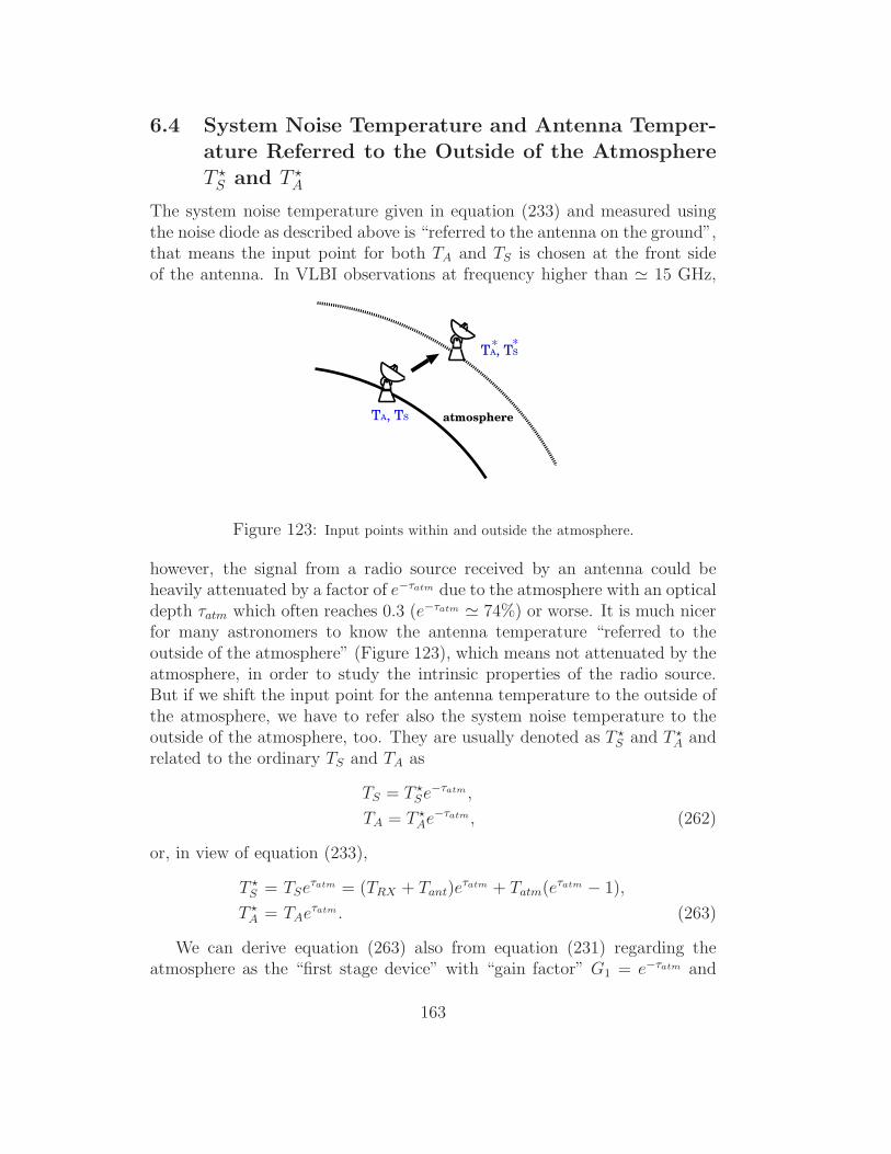
6.4 System Noise Temperature and Antenna Temper-ature Referred to the Outside of the Atmosphere

T ⋆S and T ⋆

A

The system noise temperature given in equation (233) and measured usingthe noise diode as described above is “referred to the antenna on the ground”,that means the input point for both TA and TS is chosen at the front sideof the antenna. In VLBI observations at frequency higher than ≃ 15 GHz,

atmosphereTA, TS

TA, TS* *

Figure 123: Input points within and outside the atmosphere.

however, the signal from a radio source received by an antenna could beheavily attenuated by a factor of e−τatm due to the atmosphere with an opticaldepth τatm which often reaches 0.3 (e−τatm ≃ 74%) or worse. It is much nicerfor many astronomers to know the antenna temperature “referred to theoutside of the atmosphere” (Figure 123), which means not attenuated by theatmosphere, in order to study the intrinsic properties of the radio source.But if we shift the input point for the antenna temperature to the outside ofthe atmosphere, we have to refer also the system noise temperature to theoutside of the atmosphere, too. They are usually denoted as T ⋆

S and T ⋆A and

related to the ordinary TS and TA as

TS = T ⋆Se

−τatm ,

TA = T ⋆Ae

−τatm, (262)

or, in view of equation (233),

T ⋆S = TSe

τatm = (TRX + Tant)eτatm + Tatm(eτatm − 1),

T ⋆A = TAe

τatm . (263)

We can derive equation (263) also from equation (231) regarding theatmosphere as the “first stage device” with “gain factor” G1 = e−τatm and

163

system noise tempeature TS1 = Tatm(eτatm − 1), and the receiving system asthe “second stage device” with system noise temperature TS2 = TRX + Tant.

Note that we can describe T ⋆A in terms of the brightness temperature T ⋆

B

of the source outside of the atmosphere, introduced in subsection 5.1.5, as

T ⋆A =

∮

Pn(θ, φ)T ⋆B(θ, φ) dΩ

∮

Pn(θ, φ)dΩ,

where Pn(θ, φ) is the normalized power pattern in the antenna–fixed coordi-nate system with angular variables θ and φ.

6.5 Measurement of the TS⋆

There is a clever method to directly measure the system noise temperatureT ⋆

S referred to the outside of the atmosphere. In fact, the T ⋆S can be measured

by the so–called “R–Sky” or “Room–Sky” method where the feed horn of theantenna is covered and uncovered by an absorber at the room temperatureTroom as shown in Figures 119 and 124.

TRX

Receiver system

gain G

absorber

feed horn

output

Figure 124: Measurement of the system noise temperature referred to the outside of theatmosphere by the R–Sky method.

Here we will ignore, for simplicity, the antenna noise temperature Tant inequation (233), since the ground pickup effect which contributes to the Tant

the most is kept small even at moderately low elevations in well designedradio telescope antennas with sufficiently suppressed sidelobe levels.

164

Then, when the absorber is taken off from the feed horn, the antennalooks at the blank sky and produces an output power

Wsky = kTSGB = kT ⋆Se

−τatmGB = k[TRX + Tatm(1 − e−τatm)]GB, (264)

where Tatm is the physical temperature of the atmosphere (see equations(259) and (263)). On the other hand, when the feed horn is covered by theabsorber of room temperature Troom, the output power is

Wroom = k(TRX + Troom)GB. (265)

If we adopt here a reasonable assumption that Tatm = Troom (this must becorrect with an accuracy usually better than a few percent, since both ofthem must be around 300 K), then we have

Wroom −Wsky = kTroome−τatmGB, (266)

and thereforeWsky

Wroom −Wsky

=T ⋆

S

Troom

. (267)

If we introduce a factor y now defined as

y ≡ Wroom

Wsky, (268)

we obtain the system noise temperature referred to the outside of the atmo-sphere

T ⋆S =

Troom

y − 1. (269)

Needless to say, this is another beautiful example of measuring somethingusing a calibrator.

Note that the R-Sky method gives correct T ⋆S value even when the mea-

surement is done under a radome or feed–cone cover, as far as temperatureof the cover membrane Tmem is well approximated by the room temperature(Tmem = Troom). In fact, the discussion in subsection 5.1.5 tells us that allequations from (262) to (267), and therefore equation (269), too, hold alsoin this case, if only we replace τatm by τatm + τmem, where τmem is the opticaldepth of the cover membrane as before.

6.6 Measurement of the Aperture Efficiency ηA

If we quickly switch the telescope beam between directions of a source andthe blank sky using the beam switch, we obtain output powers:

Wsource = k(TA + TS)GB = k(T ⋆A + T ⋆

S)e−τatmGB

Wsky = kTSGB = kT ⋆Se

−τatmGB. (270)

165

Then, we easily get the antenna temperature referred to the outside of theatmosphere T ⋆

A if we know the sytem noise temperature referred to the outsideof the atmosphere T ⋆

S by an equation:

T ⋆A =

Wsource −Wsky

Wsky

T ⋆S . (271)

We can measure T ⋆A in this way even when our receiving system is placed

under the radome or feed–cone cover. The only thing we have to note thenis that τatm in equation (270) should be replaced by τatm + τmem.

If the radio source observed is a standard source with known effective fluxdensity Sν and is much more compact than the beamwidth, we can calculatethe effective aperture Ae from equation (220) as

Ae = ηAAg =2kT ⋆

A

Sν, (272)

where Ag is the geometrical aperture, and therefore the aperture efficiency

ηA =2kT ⋆

A

AgSν=

8kT ⋆A

πD2Sν, (273)

where the last expression is for a circular aperture antenna with diameter D.If the source is so bright that any short term variation of the receiver gain

or the atmospheric noise can be ignored, we can just drive the telescope toswitch the directions when the beam switching mechanism is not available.

The best standard sources are bright planets like Jupiter or Venus ifthe telescope beam is not narrower than their sizes, since their brightnesstemperatures are reliably known. Strong extragalactic AGN’s like 3C84,3C273, ... could also be used if their flux densities of the date are available.

6.7 Chopper Wheel method for Precise Measurementof the Antenna Temperature T ⋆

A

In order to accurately measure the antenna temperature T ⋆A referred to the

outside of the atmosphere and aperture efficiency ηA, it is desirable to simul-taneously measure the system noise temperature T ⋆

S , too. For this purpose,one can use a method known as “absorbing disk method” or “chopper wheelmethod”. In this method, a rotating vaned–wheel like device is used in frontof the feed horn, which is much alike with the one used in the beam switch,but an absorber of the room temperature Troom is attached to one of the vanesin addition to the mirror. Thus the feed horn can now look at the sourcedirection, the mirror–reflected blank sky, and the absorber in turn within a

166

mirror

mirror

absorber

absorber

Figure 125: Absorbers and mirrors in the rotating vaned–wheel used in the chopper–wheel method.

short period of one revolution which is well less than 1 second (Figure 125).Since we now have three output powers nearly simultaneously, which aregiven by

Wsource = k[T ⋆Ae

−τatm + TRX + Tatm(1 − e−τatm)]GB,

Wsky = k[TRX + Tatm(1 − e−τatm)]GB = kT ⋆Se

−τatmGB,

Wroom = k(Troom + TRX)GB, (274)

if we again ignore the small ground pickup effect Tant, we directly obtain theantenna temperature referred to the outside of the atmosphere

T ⋆A =

Wsource −Wsky

Wroom −WskyTroom, (275)

as far as we are allowed to assume Tatm = Troom.

6.8 Measurement of the Optical Depth of the Atmo-sphere τatm — sec z Method

zenith

z

atmosphere

τatmτ0

Figure 126: sec z dependence of the optical depth τatm in the plane–parallel model ofthe atmosphere.

Elevation dependence of the attenuation of the radio signal due to theatmosphere can be well modeled by a plane–parallel atmosphere ignoring

167

the curvature of the Earth’s surface (Figure 126). In such a model, theoptical depth of the atmosphere τatm, which is approximately proportionalto the path length within the atmosphere, depends on the zenith distance z(which is an angle of a direction from the zenith, i.e. z = 90− elevation) as

τatm = τ0 sec z. (276)

Let us use the R–Sky method to measure the output powers when the feedhorn is covered and uncovered by the absorber with the room temperatureTroom. Then equations (264) and (265):

Wsky = k[TRX + Tatm(1 − e−τatm)]GB,

Wroom = k(TRX + Troom)GB.

give us, under the assumption of Troom = Tatm,

Wroom −Wsky = kTroome−τatmGB. (277)

Therefore, taking the logarithm of equation (277), we obtain

− ln(Wroom −Wsky) = τ0 sec z − ln(kTroomGB), (278)

where we used equation (276).

3.1

3.2

3.3

3.4

3.5

3.6

3.7

3.8

3.9

4

4.1

4.2

1 1.5 2 2.5 3 3.5 4

- ln

(Wab

s -

Wsk

y)

sec z

Figure 127: An example of the [− ln(Wroom − Wsky)] vs. sec z plot of measured dataobtained in a sec z measurement.

Consequently, if we measure the Wroom −Wsky at several values of zenithdistance z, and if TroomGB is nearly constant during the measurement, then

168

we can estimate the zenith optical depth τ0 as the inclination of a straightline fitted to the measured data in the [− ln(Wroom −Wsky)] vs. sec z plane,as illustrated in Figure 127.

Knowing the zenith optical depth τ0 and therefore τatm = τ0 sec z, as wellas the T ⋆

S which is also available from the R–Sky method, we can estimatethe receiver noise temperature TRX . In fact, equation (263) shows that thesystem noise temperature T ⋆

S referred to the outside of the atmosphere mustbe equal to

T ⋆S = TRXe

τatm + Troom(eτatm − 1),

when the Tant is ignored and Tatm = Troom is assumed. Therefore, if wecalculate a quantity Trcv defined by

Trcv ≡ T ⋆Se

−τatm − Troom(1 − e−τatm), (279)

using measured values of T ⋆S , τatm, and Troom, the Trcv must give a good

estimate of the receiver noise temperature TRX as far as our assumptionsare appropriate. Equation (279) is often used as a convenient way to easilyestimate the TRX and check the receiver performance.

Nevertheless, it is desirable to conduct the hot–cold measurement of thereceiver noise temperature in parallel with the sec z measurement, in orderto examine possible effect of gain variation during the sec z measurement,and also to confirm consistency of TRX values estimated in the sec z and thehot–cold methods.

Note that the sec z method gives a correct estimate of the zenith opticaldepth τ0 even when our antenna, or its feed horn, is covered by a radome orfeed–cone cover, as far as the optical depth of the cover membrane τmem doesnot depend on the zenith distance z of the antenna beam. In fact, althoughequations (277) and (278) then should be replaced by

Wroom −Wsky = kTroome−(τatm+τmem)GB,

and− ln(Wroom −Wsky) = τ0 sec z − ln(kTroome

−τmemGB),

as discussions in subsection 5.1.5 show, the straight–line fitting to the mea-sured data in the [− ln(Wroom −Wsky)] vs. sec z plane still gives correct τ0as far as e−τmem does not depend on z.

On the other hand, however, a straightforward application of equation(279) would not give a correct estimate of the actual receiver noise tempera-ture TRX when τmem is not negligiblly small. In fact, discussions in subsection

169

5.1.5 show that the system noise temperature T ⋆S referred to the outside of

the atmosphere is

T ⋆S = TS e

τatm+τmem = TRX eτatm+τmem + Troom (eτatm+τmem − 1),

in this case, as long as Tant is ignored and Tatm = Tmem = Troom is assumed.Therefore, equation (279) gives

Trcv = TRX eτmem + Troom (eτmem − 1),

and, hence, the Trcv deviates from the receiver noise temperature TRX by

Trcv − TRX = (Troom + TRX) (eτmem − 1).

For example, if Troom = 300 K, TRX = 50 K, and e−τmem = 0.92, then thedeviation reaches as large as 30 K.

It is highly desirable to regularly measure the atmospheric optical depth,

0

100

200

300

400

500

600

700

50 60 70 80 90 100

Sys

tem

Noi

se T

empe

ratu

re in

Kel

vin

Transparency of Atmosphere (%)

TRX=100KTRX=150K

Figure 128: T ⋆S – transparency e−τatm relation expected from equation (263) for two

cases of TRX = 100 K and TRX = 150 K.

hopefully every day, for statistical study of the observational condition ofthe site. In particular, it will be useful to compare the measured relationshipbetween the system noise temperature T ⋆

S and the optical depth −τatm (orthe transparency e−τatm) with the theoretical prediction which is given byequation (263) and illustrated in Figure 128. For this purpose, regular sec zmeasurements during a year or so are needed. We will then be able to see if

170

the underlying assumptions of the equation well hold and TRX is sufficientlystable for a year or so.

For efficient sec z measurements, we need a good operation software,which would point the radio telescope to desired sky directions with differentelevation angles, drive the “R–Sky” measuring instrument, read power–meteroutputs at “room” and “sky” states, plot figures such as Figure 127, calculateτatm, T ⋆

S and Trcv, and store the results to an appropriate database.

6.9 Pointing Calibration and Pointing Accuracy σθ

Even in a well manufactured antenna, the azimuth axis may not be exactlyparallel to the vertical line at the site. Likewise, the elevation axis may notbe strictly perpendicular to the azimuth axis. In the antenna specifications,tolerance values for the axis–alignments are usually set to be at 0.01 level,but such a “large” axis–offset could easily cause pointing errors (offsets) ex-ceeding the accuracy requirement of ∼ 0.1λ/D given in equation (213). Also,the gravitational yielding of the antennas causes noticeable pointing errorsmainly in the elevation direction. These pointing errors are “systematic”in the sense, that we obtain the same error values repeatedly in the samedirection of the sky. But this means that they are predictable as functionsof azimuth and elevation of the beam direction of the telescope.

Therefore, these systematic errors must be estimated and calibrated be-fore starting regular scientific observations. The pointing accuracy σθ, whichcharacterizes more or less random errors of the telescope pointing due to me-chanical inaccuracy of gears, bearings, as well as unpredictable deformationscaused by the gravity and the wind, must be determined after removing thesystematic deviations. Actually, the pointing accuracy is calculated fromthe residuals of the least–squares fitting of a number of parameters, char-acterizing systematic errors, to the measured values of the pointing errors.Hereafter, we call these parameters as “offset parameters”.

Since the offset parameters may vary in time due to the mechanical changein the antenna structure, the measurements must be repeated periodicallyonce a year or more, for keeping the best system performance.

6.9.1 Pointing Model

Let us consider a model which describes a functional dependence of the sys-tematic pointing error on the offset parameters, assuming that we observe aradio source located in azimuth Az and elevation El with an Alt–Azimuthmount antenna. Here we adopt a convention that the azimuth is measured

171

eastward from the North, i.e., Az = 0 at the North, and Az = 90 at theEast.

Following 8 quantities are usually regarded as most important offset pa-rameters for Alt–Azimuth mount antennas:

3

1

2i

i ii

i

i

4

5

6

i*

iEl

El

Az

S

E

Z

iAz

Figure 129: Unit vectors i1, · · · , i6 for describing axis–offsets of an antenna.

1. a: tilt angle of the azimuth axis in the EW direction around i1,

2. b: tilt angle of the azimuth axis in the NS direction around i2,

3. c: offset of the origin of the azimuth encoder (angle detector), plus tiltangle of the elevation axis in the azimuthal direction, around i3,

4. d: tilt angle of the elevation axis in the elevational direction around i4,

5. e: offset of the origin of the elevation encoder, plus tilt angle of thebeam axis in the elevational direction, around i5,

6. f : tilt angle of the beam axis in the azimuthal direction around i6,

7. g: cosine coefficient of the gravitational yielding in elevation,

8. h: sine coefficient of the gravitational yielding in elevation.

172

Parameters a – f represent axis offset effects, i.e., effects of misalignmentsof telescope axes, while parameters g and h represent elastic deformation ef-fects. In the present level of antenna manufacturing technology, these offsetparameters are quantities of the order of a few minutes of arc, or smaller.Therefore, it is sufficient to consider the pointing model in a linear approxi-mation with respect to the small offset parameters.

The axis–offset angles a, b, c, d, e and f correspond to small rotationangles around directions shown by the unit vectors i1, i2, i3, i4, i5 and i6 inFigure 129. Here we adopt the “right–handed screw rule” for the directionof the rotation, i.e., the positive rotation angle corresponds to the clock–wiserotation, viewed towards the direction of the unit vector.

In Figure 129, i1, i2, and i3 are basis vectors of the horizontal coordinatesystem at the antenna site. i3 is directed towards the zenith, while i1 and i2are directed towards the South and the East, respectively, in the horizontalplane. The i3 is the vertical axis, towards which the azimuth axis of theantenna must be directed in an ideal case when there is no systematic axisoffset.

i4 is directed towards azimuth Az in the horizontal plane, which is theazimuth of the radio source at the time of the observation.

i5 is chosen towards azimuth Az + 90 in the horizontal plane. The i5 isthe direction, along which the elevation axis of the antenna must be alignedin the ideal case when there is no systematic axis offset.

i6 is chosen in a direction with azimuth Az and elevation El−90, whereEl is the elevation of the radio source at the time of the observation.

i5, i6, and a unit vector i⋆, which is directed towards the radio sourcewith azimuth Az and elevation El, form a right–handed orthogonal triad.The i⋆ is the direction, towards which the beam axis of the antenna must beoriented in the ideal case when there is no systematic axis offset.

Unit vectors iAz and iEl, which are directed towards azimuthal and el-evational directions in a plane tangent to the celestial sphere at the radiosource position, are related to i5 and i6, as

i5 = iAz, (280)

i6 = −iEl, (281)

as evident from Figure 129.In the linear approximation, the pointing error ∆i⋆ is expressed in terms

of the offset of the unit vector i′⋆, which represents the direction of the actualtelescope beam axis, from the one in the desired direction i⋆:

∆i⋆ = i′⋆ − i⋆. (282)

173

The azimuthal and elevational components of the pointing error can be ex-pressed, in the linear approximation, as:

cosEl∆Az = ∆i⋆ · iAz,

∆El = ∆i⋆ · iEl. (283)

These are the quantities which we can measure in “pointing measurements”,as we will see later.

Now let us derive the functional dependence of these azimuthal and ele-vational components of the pointing error on the offset parameters, which isnothing but the pointing model we are looking for.

In the linear approximation, we can separately consider the effects of theaxis offsets and the elastic deformation, and then sum up the results to obtainthe total effect. Therefore, we first consider the axis offset effects, assumingthat the radio telescope antenna is a rigid body.

From the theory of the rotational dynamics of the rigid body, we knowthat, if a rigid body rotates around an axis i, where i is a unit vector, by asmall angle ∆θ, any vector x fixed to the rigid body is displaced by:

∆x = ∆θ i × x, (284)

in a linear approximation with respect to ∆θ. We can introduce here a vectorof small angle rotation ∆Θ as:

∆Θ = ∆θ i. (285)

Then, equation (284) can be expressed as

∆x = ∆Θ × x. (286)

It is known that the vectors of small angle rotations can be summed up asordinary vectors in the linear approximation with respect to the small angles.Since, in our present problem, a rotational displacement of the radio telescopeantenna is composed of rotations by small angles a, b, · · · , f around the sixunit vectors i1, i2, · · · , i6, the total rotation angle vector of the antenna ∆Θis expressed by:

∆Θ = ai1 + bi2 + ci3 + di4 + ei5 + fi6. (287)

The angular offset of the telescope beam axis ∆ia⋆ from the desired direc-

tion i⋆, due to the superposed axis offset effects, is then expressed as:

∆ia⋆ = ∆Θ × i⋆. (288)

174

Now, it is evident from Figure 129 and equations (280), (281) that

i3 = sinEl i⋆ + cosEl iEl, (289)

i4 = cosEl i⋆ − sinEl iEl, (290)

and

i1 = cos(180 −Az) i4 + sin(180 − Az) i5

= − cosAz i4 + sinAz i5

= − cosAz cosEl i⋆ + cosAz sinEl iEl + sinAz iAz, (291)

i2 = sin(180 −Az) i4 − cos(180 −Az) i5

= sinAz i4 + cosAz i5

= sinAz cosEl i⋆ − sinAz sinEl iEl + cosAz iAz. (292)

Taking into account that

i⋆ × i⋆ = 0,

iAz × i⋆ = iEl, (293)

iEl × i⋆ = −iAz,

we obtain, from equations (280), (281), (289), (290), (291), and (292),

i1 × i⋆ = − cosAz sinEl iAz + sinAz iEl, (294)

i2 × i⋆ = sinAz sinEl iAz + cosAz iEl, (295)

i3 × i⋆ = − cosEl iAz, (296)

i4 × i⋆ = sinEl iAz, (297)

i5 × i⋆ = iEl, (298)

i6 × i⋆ = iAz. (299)

Therefore, in view of equations (287) and (288), we have the following ex-pression for the beam offset due to the axis offset effects:

∆ia⋆ = ∆Θ × i⋆

= a (− cosAz sinEl iAz + sinAz iEl)

+b (sinAz sinEl iAz + cosAz iEl)

−c cosEl iAz + d sinEl iAz + e iEl + f iAz. (300)

Consequently, we obtain the azimuthal and elevational components of thebeam offset due to the axis offset effects, using equation (283),

cosEl∆Aza = ∆ia⋆ · iAz

= −a cosAz sinEl + b sinAz sinEl − c cosEl + d sinEl + f,

∆Ela = ∆ia⋆ · iEl

= a sinAz cosAz + b cosAz + e. (301)

175

The main terms of the elastic deformation effect, which are the cosine andsine of elevation terms due to the gravitational yielding of the radio telescopeantenna, are just added to the elevational component of the above equations(301), and therefore, we obtain the total beam offset:

cosEl∆Az = −a cosAz sinEl + b sinAz sinEl − c cosEl + d sinEl + f,

∆El = a sinAz cosAz + b cosAz + e+ g cosEl + h sinEl. (302)

Note that signs of the terms in the above equations may differ in differentliterature, depending on senses of the rotation angles.

6.9.2 Pointing Measurement

Now, if we measure the azimuthal and elevational offsets of the actual beamdirection from the desired one at many directions, we can fit the equation(302) to the measured values to estimate the 8 parameters from a to g and,from the residuals, the pointing accuracy σθ, by the method of the leastsquares. An example of the sky coverage of the water maser sources observedin a pointing measurement at 22 GHz is shown in Figure 130.

0

10

20

30

40

50

60

70

80

90

0 100 200 300 400

EL

[deg

]

AZ [deg]

Figure 130: An example of the sky coverage of the sources in a pointing measurement.

Sometimes it is difficult to solve all 8 parameters due to the strong cor-relations among some of the parameters. In such a case, we have to assumereasonable values for some of the parameters and solve the least squaresequations for rest of the parameters.

It is empirically known, for some of the wheel & track type antennas,that inclusion of additional terms with cos(2Az) and sin(2Az) dependencesinto the pointing model better fits the results of the pointing measurements.

176

In such a case, we have to increase the number of offset parameters to 12, orso.

The measurements are usually conducted by so–called “5 points scan”method. In this method, power from a radio source with well determinedcelestial position is measured at a telescope direction determined by a certainset of values of the azimuth– and elevation encoders (or angular scales) of thetelescope, which are predicted by the source tracking software and instructedby the antenna control software, and at 4 more directions in North, South,East and West sides of the instructed one with the angular separation ofroughly a half of the HPBW (Figure 131).

0.5 HPBW

Figure 131: 5 points scan.

Given that the celestial positions and predicted Az and El values areaccurate enough (at a level better than 1 arcsecond, say), the power mustbe strongest at the instructed direction and equally lower at four other di-rections, if the telescope does not have any systematic axis–offsets and grav-itational yielding. If not, however, we will get an asymmetrical distributionof the measured powers at the 5 points. It is a usual practice to fit a two–dimensional Gaussian beam model to the measured power values to derivethe offsets cosEl∆Az and ∆El between the actual and required beam di-rections which will be fitted by the model given in equation (302).

To achive the required accuracy of the prediction, the source trackingsoftware must properly take into account major astrometric and geophysicaleffects including the abberation, the precession–nutation and the atmosphericrefraction effects.

The radio sources used for the pointing measurements must be compact,strong enough, and must have well determined values of the position co-ordinates. Strong astronomical maser sources are often used for frquencybands, where such masers are available. For maser sources, we can easilyobtain the antenna temperature value by comparing the “in–line” part andthe “out–of–line” part of the frequency spectrum, as shown in Figure 132.

177

For other frequency bands, strong continuum sources such as quasars or su-pernova remnants are used with appropriate antenna temperature measuringinstruments.

For efficient pointing measurements, we need a good scheduling softwareand a well automated antenna operation software, which would enable usto quickly observe “pointing sources” one by one at different sky directions,

Figure 132: 5 points scan result at 43 GHz for SiO maser source R Cas obtained at Irikistation of VERA which shows southward offset of the beam.

performing 5 points scans and automatically getting pointing offset valuesby the Gaussian fitting. In the case of the maser sources, we must correctlychoose the “in–line” frequency range of the maser spectrum, where a desiredline component is located. Since the range periodically shifts in frequencydue to the Doppler effect assocaited with the orbital motion of the Earth, weneed a software which calculates the “in–line” frequency range of date, fromthe local–standard–of–rest frequency value (or from the radial velocity vLSR,

178

referred to the Local Standard of Rest).In massive star forming regions, maser features are often spread over a

wide area of the sky, exceeding tens of arcseconds in size. Therefore, we haveto choose the “in–line” range, so that it covers a strong maser feature orfeatures, which are concentrated within a compact region much smaller thanthe antenna beam.

6.10 Beam Pattern Measurement

Power pattern of an antenna beam can be derived by measuring receivedpower (or antenna temperature) of a compact strong radio source, in terms ofthe “grid–mapping” method (Figure 134) or the “drift–scan” method (Figure133).

Figure 133: Beam patterns obtained with the drift–scan method at 22 GHz (Top) andat 43 GHz (Bottom) (courtesy of the VERA group, 2002).

In the grid–mapping method, the received power values are measured atcenters of a number of grids in the sky, chosen around the source with equalspacing, typically corresponding to a half of the expected beam size, in rightascension and declination. The results are analyzed with standard single–dish imaging softwares, and two–dimensional beam patterns are obtained.An example is shown in the lower panel of Figure 134.

In the drift–scan method, the received power is measured while a sourcepasses in front of the antenna beam due to the diurnal motion, or whenthe antenna is driven, so that the beam crosses the source in azimuth andelevation directions. In this case, one dimensional beam pattern, as shownin Figure 133, is obtained at each scan.

179

Figure 134: Grid–mapping method for beam pattern measurement (Top), and a resul-tant beam pattern (Bottom) (courtesy of the VERA group, 2004).

180

In the both methods, the antenna pointing must be well calibrated, andradio source positions must be precisely known. Also, the measurements mustbe done within a short time under the clear sky, in order to avoid atmosphericdisturbances. It is highly desirable to have automated antenna–operation,data acquisition and analysis softwares for the beam pattern measurements.

References

Adachi, S., 1985, Electromagnetic Wave Engineering, Korona-

sha, (in Japanese).Kraus, J.D., 1984, Electromgnetics, 3rd Edition, McGraw–Hill

(Singapore).Kraus, J.D., 1986, Radio Asronomy, 2nd Edition, Cygnus–Quasar

Books.Nyquist, H., 1928, Thermal Agitation of Electric Charge in Con-

ductors, Phys. Rev., 32, 110–113.Panofsky, W.K.H., and Phillips, M., 1962, Classical Electricity

and Magnetism, 2nd Edition, Dover Publications, Inc. (NewYork).

Rohlfs, K., 1986, Tools of Radio Astronomy, Springer–Verlag

(Berlin).Rohlfs, K., and Wilson, T. L., 2000, Tools of Radio Astronomy,

3rd Edition, Springer–Verlag (Berlin).

181