radio resource allocation in relay based ofdma...
TRANSCRIPT

Radio Resource Allocation in Relay Based OFDMA Cellular Networks
Lin Xiao
Submitted for the degree of Doctor of Philosophy
School of Electronic Engineering and Computer Science
Queen Mary, University of London
January 2010

2
To all the people I love

3
Abstract
Adding relay stations (RS) between the base station (BS) and the mobile stations (MS)
in a cellular system can extend network coverage, overcome multi-path fading and
increase the capacity of the system.
This thesis considers the radio resource allocation scheme in relay based cellular
networks to ensure high-speed and reliable communication. The goal of this research
is to investigate user fairness, system throughput and power consumption in
wireless relay networks through considering how best to manage the radio resource.
This thesis proposes a two-hop proportional fairness (THPF) scheduling scheme fair
allocation, which is considered both in the first time subslot between direct link users
and relay stations, and the second time subslot among relay link users.
A load based relay selection algorithm is also proposed for a fair resource allocation.
The transmission mode (direct transmission mode or relay transmission mode) of
each user will be adjusted based on the load of the transmission node.
Power allocation is very important for resource efficiency and system performance
improvement and this thesis proposes a two-hop power allocation algorithm for
energy efficiency, which adjusts the transmission power of the BS and RSs to make
the data rate on the two hop links of one RS match each other.
The power allocation problem of multiple cells with inter-cell interference is studied.
A new multi-cell power allocation scheme is proposed from non-cooperative game
theory; this coordinates the inter-cell interference and operates in a distributed
manner. The utility function can be designed for throughput improvement and user
fairness respectively.
Finally, the proposed algorithms in this thesis are combined, and the system
performance is evaluated. The joint radio resource allocation algorithm can achieve a
very good tradeoff between throughput and user fairness, and also can significantly
improve energy efficiency.

4
Acknowledgement
I would like to express my gratitude to all those who helped me to complete this
research.
The first person I want to say “thank you” to is my supervisor Prof Laurie Cuthbert.
During my PhD time, he gave me the strongest support and guidance for both my
study and daily life. He gave me lots of freedom to study an area that interested me
and he encouraged every small progress I have ever made. His selflessness, goodness
to students, and passion for the work is the treasure that I value for the rest of my life.
I would also like to express my appreciation to Dr Yue Chen and Dr John Schormans
for their helpful suggestions and comments on my research. Yue Chen, who is my
second supervisor, is a nice, beautiful, and smart woman who gave me a lot of useful
advice during my study. John Schormans gave me his support and encouragement,
boosting my confidence and helping me to finish the study well.
Finishing a PhD degree abroad is not easy, but because of the company of my lovely
friends, the memory of the last three years is so beautiful and colourful. Thanks
Keijing Zhang, Luo Liu, Dapeng Zhang, Xiaojing Wang, and so many others. You are
my best friends forever.
In my life, there are so many people I should thank. The love they have given me is
enormous and selfless. With my love and gratitude, I want to dedicate this thesis to
all the people who have ever helped me.

5
Contents
List of Figures 8
List of Abbreviations 11
Chapter 1 Introduction 14
1.1 Background/Motivation 14
1.2 Research Scope 15
1.3 Research Contributions 16
1.4 Author’s Publications 18
1.5 Thesis Organisation 19
Chapter 2 Relay based OFDMA Cellular Networks 20
2.1 Basic Concept of Relay 20
2.2 Usage Model of Relay 21
2.3 Classification of Relay 232.3.1 Amplify-Forwarding and Decode-Forwarding 232.3.2 Fixed Relay and Mobile Relay 23
2.4 Relevant Research 25
2.5 Orthogonal Frequency Division Multiple Access 272.5.1 Principle of OFDMA 272.5.2 OFDMA System Model 292.5.3 Advantages of OFDMA 30
2.6 Deployment of Fixed Relay in OFDMA Cellular Systems 312.6.1 Hops between BS and MS 312.6.2 Definition of Terms 322.6.3 Frame Structure 322.6.4 Frequency Band 342.6.5 Frequency Reuse Method 342.6.6 Distance between BS and RS 35
2.7 Summary 36
Chapter 3 Simulator for OFDMA Relay Networks 37
3.1 Overall Design of Simulation Platform 37
3.2 Simulator System Parameters 39
3.3 Module Functions and Implementation 413.3.1 Initialisation Module 413.3.2 CQI Feedback Module 42

6
3.3.3 Resource Allocation Module 43
3.4 Channel Module 443.4.1 Pathloss Model 443.4.2 Shadow Fading Model 473.4.3 Multi-pathFading Model 47
3.5 Verification and Validation 483.5.1 Verification of Relay Location and MS Distribution 483.5.2 Verification of Channel States 493.5.3 Verification of Number of Drops 51
3.6 Summary 53
Chapter 4 Radio Resource Allocation in OFDMA Relay Networks 54
4.1 Introduction to Radio Resource Management 54
4.2 Relay Selection 56
4.3 Channel Allocation 58
4.4 Power Allocation 60
4.5 Summary 61
Chapter 5 Fair Subchannel Allocation and Relay Selection 62
5.1 Introduction 62
5.2 System Model 625.2.1 System Parameters 625.2.2 Channel Capacity 635.2.3 Optimization Problem 65
5.3 Two-Hop Proportional Fairness Algorithm 665.3.1 Algorithm Description 665.3.2 Algorithm Procedure 695.3.3 Performance Simulation and Analysis 70
5.4 Load Based Relay Selection Algorithm 765.4.1 Algorithm Description 775.4.2 Algorithm Procedure 825.4.3 Performance Simulation and Analysis 83
5.5 Summary 87
Chapter 6 Energy Efficient Power Allocation 89
6.1 Introduction 89
6.2 Power Allocation between Two-Hops 896.2.1 Existing problem 896.2.2 Two-Hop Power Allocation 91

7
6.2.3 Performance Simulation and Analysis 94
6.3 Power Allocation among Multi-Cells 976.3.1 Background of Game Theory 976.3.2 Multi-Cell System Model 996.3.3 Non-Cooperative Power Allocation Game 1026.3.4 Non-Cooperative Power Allocation Game for Fairness 116
6.4 Joint Power Allocation of THPA and NPAG 1236.4.1 Algorithm Procedure 1236.4.2 Performance Simulation and Analysis 124
6.5 Summary 127
Chapter 7 Joint Radio Resource Allocation Algorithm 128
7.1 Performance Comparison using the NPAG variants 1297.1.1 Performance Comparison between LRTN, PRNG and PREQ 1297.1.2 Performance Comparison between LTTN, PTNG and PTEQ 1347.1.3 Performance Comparison between LRTN and LTTN 138
7.2 Performance Comparison using the NPAG-F variants 138
7.3 Performance Comparison between LTTN and LTTN-F 141
7.4 Summary 142
Chapter 8 Conclusions and Future work 143
8.1 Specific conclusions 143
8.2 Future work 144
References 146

8
List of Figures
Figure 2.1 Example fixed infrastructure usage model 21
Figure 2.2 Examples of temporary coverage 22
Figure 2.3 Typical applications in fixed relaying system 24
Figure 2.4 Orthogonal subcarriers 28
Figure 2.5 OFDM transmitter and receiver 28
Figure 2.6 Definition of terms in relay network 32
Figure 2.7 The DL transparent frame structure in relaying system 33
Figure 2.8 The DL non-transparent frame structure in relaying system 33
Figure 2.9 Frequency reuse method 35
Figure 3.1 Flow chart of simulator 39
Figure 3.2 Flow chart of initial module 42
Figure 3.3 Flow chart of CQI feedback module 42
Figure 3.4 Flow chart of resource scheduling module 43
Figure 3.5 BS-RS link with LOS 44
Figure 3.6 Distribution of MSs and RSs in multi-cell system 49
Figure 3.7 Verification of large scale channel fading between BS and MS 50
Figure 3.8 Verification of fast fading channel 51
Figure 3.9 System throughput vs. number of drops 52
Figure 3.10 System throughput vs. number of users 53
Figure 5.1 Layout of single cell relay based OFDMA network 70
Figure 5.2 System throughput vs. RS normalized distance 73
Figure 5.3 Fairness index vs. RS normalized distance 74
Figure 5.4 System throughput vs. number of users 75
Figure 5.5 Fairness index vs. number of users 75
Figure 5.6 Traffic load of uniform distribution 84
Figure 5.7 System throughput comparison in uniform distribution 85
Figure 5.8 User fairness comparison in uniform distribution 85
Figure 5.9 Traffic load of hotspot scenario 86
Figure 5.10 System throughput comparison in hotspot scenario 86
Figure 5.11 Fairness index comparison in hotspot scenario 87
9
Figure 6.1 Two-hop throughput of RS with equal power allocation 90
Figure 6.2 Two-hop throughput of RS with THPA 94
Figure 6.3 BS/RS transmission power vs. RS normalized distance 96
Figure 6.4 Total transmission power vs. RS normalized distance 96
Figure 6.5 Downlink inter-cell interference in the second hop link 99
Figure 6.6 Layout of multi-cell system 100
Figure 6.7 The second hop average throughput vs. RS basic pricing factor 110
Figure 6.8 RS power vs. RS basic pricing factor 110
Figure 6.9 System throughput vs. BS basic pricing factor (fixed RS pricing factor) 111
Figure 6.10 User fairness vs. BS basic pricing factor (fixed RS pricing factor) 112
Figure 6.11 BS power vs. BS basic pricing factor (fixed RS pricing factor) 112
Figure 6.12 System throughput vs. number of users in each cell 114
Figure 6.13 Transmission power vs. number of users in each cell 114
Figure 6.14 Fairness index vs. number of users in each cell 115
Figure 6.15 System throughput vs. BS basic pricing factor 120
Figure 6.16 User fairness vs. BS basic pricing factor 121
Figure 6.17 BS transmission power vs. BS basic pricing factor 121
Figure 6.18 RS transmission power vs. BS basic pricing factor 122
Figure 6.19 System throughput vs. number of users in each cell 125
Figure 6.20 BS transmission power vs. number of users in each cell 126
Figure 6.21 RS transmission power vs. number of users in each cell 126
Figure 7.1 System throughput vs. BS basic pricing factor 130
Figure 7.2 User fairness vs. BS basic pricing factor 131
Figure 7.3 BS transmission power vs. BS basic pricing factor 132
Figure 7.4 RS transmission power (all 6 RS) vs. BS basic pricing factor 132
Figure 7.5 Total transmission power vs. BS basic pricing factor 133
Figure 7.6 Performance change relative to LRTN for PREQ 134
Figure 7.7 Average throughput vs. BS basic pricing factor 135
Figure 7.8 User fairness vs. BS basic pricing factor 135
Figure 7.9 BS transmission power vs. BS basic pricing factor 136
Figure 7.10 RS transmission power vs. BS basic pricing factor 136
Figure 7.11 Total transmission power vs. BS basic pricing factor 137

10
Figure 7.12 Performance improvement of LTTN over PTEQ 137
Figure 7.13 Comparison between LRTN and LTTN based on same throughput 138
Figure 7.14 Comparison between LRTN-F, PRNG-F and PREQ 139
Figure 7.15 Comparison between LTTN-F, PTNG-F and PTEQ 140
Figure 7.16 Comparison for the NPAG-F variants 141
Figure 7.17 Comparison between LTTN and LTTN-F 142

11
List of Abbreviations
3G Third Generation
3GPP The 3rd Generation Partner Project
AF Amplify and Forwarding
ART Above Roof Top
AWGN Additive White Gaussian Noise
BER Bit Error Rate
BRT Below Roof Top
BS Base Station
BW Bandwidth
CDF Cumulative distribution Function
CP Cyclic Prefix
CQI Channel Quality Indicator
CSI Channel State Information
DACs Digital-to-Analogue Converters
DF Decode and Forwarding
DFT Discrete Fourier Transform
DL Downlink
DMPA Distributed Multi-cell Power Allocation
EQPA Equal Power Allocation
EU European Union
E-UTRAN Evolved UMTS Terrestrial Radio Access Network
FDD Frequency Division Duplex
FDM Frequency-Division Multiplexing
FFT Fast Fourier Transform

12
FP 6 Framework Programmes 6
FRF Frequency Reuse Factor
HDR High Data Rate
ICI Inter-carrier Interference
IDFT Inverse Discrete Fourier Transform
IEEE The Institute of Electrical and Electronics Engineers
IFFT Inverse Fast Fourier Transform
ITU-R International Telecommunications Union Radio communication sector
LBRS Load Based Relay Selection
LOS Line-of-Sight
LRTN Joint Algorithm of LBRS, RR, THPA, NPAG
LRTN-F Joint Algorithm of LBRS, RR, THPA, NPAG-F
LTE Long Term Evolution
LTE-A Long Term Evolution Advanced
LTTN Joint Algorithm of LBRS, THPF, THPA, NPAG
LTTN-F Joint Algorithm of LBRS, THPF, THPA, NPAG-F
Max C/I Maximum carrier to interference ratio
MIMO Multiple Input Multiple Output
MS Mobile Station
NLOS Non-Line-of-Sight
NPAG Non-cooperative Power Allocation Game
NPAG-F Non-cooperative Power Allocation Game for Fairness
NP-hard Non-deterministic Polynomial-time hard
OFDM Orthogonal Frequency Division Multiplexing
OFDMA Orthogonal Frequency Division Multiplexing Access

13
PBRS Pathloss Based Relay Selection
PF Proportional Fairness
PPF Partial Proportional Fairness
PREQ Joint algorithm of PBRS, RR, EQPA
PRNG Joint algorithm of PBRS, RR, NPAG
PRNG-F Joint algorithm of PBRS, RR, NPAG-F
PSK Phase Shift Keying
PTEQ Joint algorithm of PBRS, THPF, EQPA
PTNG Joint algorithm of PBRS, THPF, NPAG
PTNG-F Joint algorithm of PBRS, THPF, NPAG-F
QAM Quadrature Amplitude Modulation
QoS Quality of Service
RAOS Relay Aided Opportunistic Scheduling
RR Round Robin scheduling algorithm
RRM Radio Resource Management
RS Relay Station
SINR Signal to Interference plus Noise Ratio
TDD Time Division Duplex
TG Time Guard
THPA Two-Hop Power Allocation scheme
THPF Two-Hop Proportional Fairness scheme
TTI Transmission Time Interval
UL Uplink

14
Chapter 1 Introduction
1.1 Background/Motivation
As wireless communication develops, higher requirements are demanded of wireless
networks. In 2003, the International Telecommunication Union Radio
communication sector (ITU-R) proposed that next generation networks should
achieve a total cell capacity of up to 1 Gbps for slow-moving users and 100 Mbps for
fast moving mobile stations (MS). However, the limitation on radio resource is the
real bottleneck for developing higher-speed wireless networks. Research on future
wireless systems to provide higher capacity, yet retaining efficient use of the
frequency spectrum, can be divided into two aspects:
i. Advanced technology in the physical layer,such as orthogonal frequency
division multiplexing (OFDM) [1] which can be used to reduce multi-path
interference, and multiple input multiple output (MIMO) [2], which provides
spatial reuse.
ii. New network architectures, such as adding relay stations between the base
station (BS) and MS [3], or with MESH networks [4].
In future wireless systems, each user will expect a high throughput so they can
access different multimedia services regardless of their location and mobility.
However, the traditional cellular architecture is not well-suited to provide uniform
data rate coverage. Additionally, if the radio propagation is non-line-of-sight (NLOS)
(as is likely) the pathloss will be higher than line-of-sight (LOS), so that the effect on
an MS near the cell boundary will be worse, making it more difficult to achieve a
spectral efficiency comparable to that seen by an MS near the BS that does have LOS
transmission.
A simple way to handle the pathloss problem is to divide a long path into multiple
shorter hops and to use relay stations (RS) for data forwarding. RSs can also be used

15
for temporary coverage in applications such as disaster relief as well as being
deployed in hotspot areas.
Whatever techniques are used for increasing available bit rate, radio resource
management (RRM) is an increasingly important problem and one that faces new
challenges. In addition, the spectral efficiency and the energy efficiency should be
considered in the RRM. The addition of relay stations in the wireless cellular network
creates new research issues for the RRM, including relay station allocation, handover
between RSs, and new considerations in frequency planning. In addition, channel
allocation and power allocation between relays need to be considered.
1.2 Research Scope
This thesis describes research into the radio resource allocation scheme in relay based
cellular networks. OFDMA [5] will be the modulation and multiple access method
for future wireless networks and hence it is the only multiple access method
considered in this thesis.
Adding fixed relays into the cellular network adds new research considerations:
• which users will have their data forwarded through a relay;
• which relay will be selected to serve a user;
• the allocation of subchannels to the RS and MS in the first hop link;
• the allocation of subchannels to the MS in the second hop link;
• how to allocate transmission power between links; and
• how to allocate transmission power among cells.
The goal of this research is to investigate fairness, throughput and power
consumption of wireless relay networks through considering how best to manage the
radio resource.
Initially fairness is considered as it is important that available resources are shared
equitably between users. The user fairness is considered in the subchannel allocation

16
and relay selection, which will give the best tradeoff between system throughput and
user fairness.
Power allocation is very important for resource efficiency and system performance.
Determining how transmission power will be allocated between the two hop links
and among different cells is important to increase the power efficiency while
maintaining system performance.
1.3 Research Contributions
The work reported in this thesis is novel. The main contributions are:
1. Two-hop proportional fairness algorithm
This thesis proposes a two-hop proportional fairness (THPF) scheduling scheme for
relay based OFDMA cellular systems. The fairness allocation problem is considered
both in the first time subslot between direct link users and relay stations, and the
second time subslot among relay link users. The proportional fairness scheduling
algorithm [6] is extended to a two-hop scenario, so the long-term fairness between
the relay link user and the direct link user is guaranteed, and the radio resource is
fully exploited.
2. Load based relay selection algorithm
A load based relay selection algorithm (LBRS) is proposed for a fair resource
allocation. The transmission mode (direct transmission mode or relay transmission
mode) of each user will be adjusted based on the load of the transmission node,
which will make the long-term average data rate of relay link users and direct link
users equal so that user fairness is enhanced.
3. Two-hop power allocation algorithm
An adaptive power allocation algorithm (called two-hop power allocation - THPA) is
proposed for energy efficiency in relay based OFDMA cellular systems. The base

17
station or relay station adjusts power adaptively in terms of the difference between
the first hop link data rate and the second hop link data rate of each RS. In this way,
the data rate on the two hop links of one RS will be matched so that the total
transmission power will be reduced while the system throughput does not decrease.
4. Multi-cell non-cooperative power allocation game
A multi-cell non-cooperative power allocation game (NPAG) is proposed to improve
the system throughput and reduce the transmission power. This is applied to the first
time subslot for BSs and the second time subslot for RSs. In all the cells, each
transmitter (BS or RS) controls the power allocation on each subchannel to maximize
its own utility in a distributed way. As the Nash equilibrium is used to determine the
solution of this problem, the existence and uniqueness of the Nash equilibrium are
also studied.
5. Multi-cell non-cooperative power allocation game for fairness
The multi-cell non-cooperative power allocation game is modified by adding a novel
utility function defined for user fairness, since cell-edge users will suffer from larger
inter-cell interference. This is known as NPAG-F. The pricing factors for BS and RS
are adjusted adaptively as a function of the average data rate and it is shown that this
improves fairness greatly with only a small impact on system throughput and
reduces the transmission power of the BS and the RSs greatly.
6. Joint radio resource allocation algorithm
The proposed algorithms in this thesis improve the system performance by relay
selection, subchannel allocation and power allocation. The proposed LBRS, THPF,
THPA and NPAG (NPAG-F) are combined, and the system performance
(throughput, the user fairness and energy efficiency) is evaluated. The joint radio
resource allocation algorithm can achieve a very good tradeoff between throughput
and user fairness, and also can significantly improve energy efficiency.

18
1.4 Author’s Publications
[1] Lin Xiao, Laurie Cuthbert. “A Two-hop Proportional Fairness Scheduling
Algorithm for Relay Based OFDMA Systems”, in IEEE WICOM 2008, Oct.10, 2008,
pp. 1-4.
[2] Lin Xiao, Laurie Cuthbert. “Improving Fairness in Relay-based Access Networks”,
in ACM MSWIM 2008, Nov. 2008, pp. 18-22.
[3] Lin Xiao, Laurie Cuthbert. “Power Allocation Scheme in Regenerative Relay-
based OFDMA Systems”, in IEEE ICCS 2008, Nov. 2008, pp. 637-641.
[4] Lin Xiao, Laurie Cuthbert. “Load Based Relay Selection Algorithm for Fairness in
Relay Based OFDMA Cellular Systems”, in IEEE WCNC 09, Apr. 2009, pp. 1-6.
[5] Lin Xiao, Laurie Cuthbert. “Multi-cell Non-cooperative Power Allocation Game in
Relay Based OFDMA Systems”, in IEEE VTC2009-Spring, Apr. 2009, pp. 1-5.
[6] Lin Xiao, Laurie Cuthbert, Tiankui Zhang. “Distributed Multi-cell Power
Allocation Algorithm for Energy Efficiency in OFDMA Relay Systems”, in IEEE
ICC Workshops '09, Jun. 2009, pp. 1-5.
[7] Lin Xiao, Laurie Cuthbert, Tiankui Zhang. “User Fairness Analysis of a Game
Theory Based Power Allocation Scheme in OFDMA Relay Systems”, in European
Wireless 2009, May 2009, pp. 173-177.
[8] Lin Xiao, Tiankui Zhang, Yutao Zhu, Laurie Cuthbert. “Two-Hop Subchannel
Scheduling and Power Allocation for Fairness in OFDMA Relay Networks”, in
ICWMC 2009, Aug. 2009, pp. 267-271.
[9] Lin Xiao, Yue Chen, Tiankui Zhang, Laurie Cuthbert. “Multi-cell Non-
cooperative Power Allocation Game for User Fairness in OFDMA Relay Systems”,
in WPMC'09, 2009.

19
1.5 Thesis Organisation
The remainder of this thesis is organised as follows.
Chapter 2 introduces the relevant concepts in relay networks, including the basic
concept of a relay based cellular network, usage model, relay classification and
network configuration; it also introduces relevant research in relay networks.
Chapter 3 discusses the simulator used for relay based OFDMA systems. The overall
design of the simulation platform and the system parameters are given in the first
part of this chapter with the detailed function of the main modules being given in the
second part. The chapter also discusses validation of the simulator.
Chapter 4 surveys radio resource allocation in relay networks. The basic concept and
content of resource management is introduced first, and then the relevant work of
relay selection, channel allocation and power allocation is discussed in turn.
Chapter 5 investigates the fairness issue for resource allocation in two-hop relay
based cellular systems. A two-hop proportional fairness scheduling algorithm and a
load based relay selection algorithm are proposed to give fair resource allocation.
Chapter 6 researches the power allocation problem. First, a two-hop power allocation
scheme for energy saving is given that balances the date rates on the two hop links.
Second, the power allocation problem with co-channel interference is studied in
multi-cell systems. Based on game theory, a multi-cell non-cooperative power
allocation game for throughput and fairness is proposed respectively. Besides, the
joint power allocation algorithm which considered power allocation between multi-
cell and between two hop links is given and the performance is discussed.
Chapter 7 gives the system performance evaluation of the proposed radio resource
allocation algorithms in this thesis.
Chapter 8 concludes the works in this thesis, and the direction of the future work is
discussed.

20
Chapter 2 Relay based OFDMA Cellular Networks
2.1 Basic Concept of Relay
In future wireless systems, the requirement for high data rate and spectral efficiency
means that the conventional cellular architecture is not feasible for the following
reasons:
• Much higher transmission power is needed to maintain the same coverage
because the required transmission rate is much higher to support applications.
• The frequency spectrum will be higher than the 2GHz band and as a result
the radio propagation will be significantly more vulnerable to NLOS
conditions [7].
To overcome these problems, some fundamentally new technologies are needed to
satisfy the requirement of throughput and coverage: these include modification of
wireless network architecture as well as advanced transmission techniques.
Increasing the density of base stations is one potential solution for these two
problems but it will greatly increase the deployment costs; an alternative is
deploying RS which has drawn much attention [7] and is considered to be a most
promising architecture for the very high throughput and coverage requirements of
future systems. Adding RS in a cellular system can extend network coverage,
overcome multi-path fading and increase the capacity of the system.
RSs, which can be either network elements or user terminals, are more intelligent
than repeaters and are capable of storing and forwarding data, making scheduling
and routing decisions, supporting radio resource assignment and MS handover [8].
The cost of a relay network is much lower compared with one that just adds more
BSs because RSs have more limited functionality. Compared with single-hop cellular
networks in which data is transmitted directly between BS and MS, information can

21
be routed from source to destination via multiple hops in relay based cellular
networks.
2.2 Usage Model of Relay
Different models can be devised for how relay networks can be used; all of those
mentioned are from [9].
In the fixed usage model, fixed RSs can be sited on towers, poles, buildings, lamp
posts, or other similar locations. Figure 2.1 (Figure 1 from [9]) illustrates some of the
cases that appear in this usage model:
• deployment of RSs to provide coverage extension at the edge of the cell;
• coverage for indoor locations;
• coverage for users in “holes” that exist due to shadowing and in areas
between buildings; and
• access for clusters of users outside the coverage area of the BS.
Figure 2.1 Example fixed infrastructure usage model (from [9])

22
Another model is for in-building coverage where RSs are used to provide better
coverage and higher throughput inside a closed area, like a building or shopping
mall; RSs can be fixed or nomadic and can be inside or outside the building.
In the temporary coverage model, nomadic RSs are put in temporary locations, to
provide capacity where the BS and fixed RS will not suffice. Some examples of this
usage model are (i) emergency or disaster recovery; (ii) temporary coverage for event,
which is illustrated in Figure 2.2 (Figure 3 from [9]).
Figure 2.2 Examples of temporary coverage (from [9])
Mobile RSs can also be located on a mobile vehicle, such as a bus, train or ferry and
provide service directly to a number of MSs which are travelling together with the
mobile vehicle. In this case the RSs are mobile in the sense that they are moving with
the vehicle, but they are fixed relative to the MSs. RSs deployed in this usage model
are expected to be complex as they may enter and exit the network when the vehicle
enters or exits the coverage area of the network. In this model, topologies may be
more than two-hops. An example of a multi-hop topology is the case where the train

23
travels through a tunnel and the mobile RS onboard the train connects to RSs that are
deployed along the tunnel [9].
2.3 Classification of Relay
2.3.1 Amplify-Forwarding and Decode-Forwarding
RSs can be classified into amplify-forwarding (AF) relay and decode-forwarding (DF)
relay.
The AF relay receives the useful signals from the transmitter with interference plus
noise; then it simply amplifies the received signals and retransmits them. The
receiver can selectively receive either the retransmitted signal from the RS or the
signal from the BS directly; it can even combine both of the signals. Although the
noise is amplified by the RS, the system performance can still be improved by the AF
relay using selective receiving or combined receiving [10].
A DF relay is a RS that can decode and regenerate the received signal so that it does
not retransmit the received noise, although the system time delay is longer than that
with the AF scheme [11].
Other relay types exist, including the compress and forwarding (CF) relay that
compresses and forwards to reduce the data to be retransmitted [11].
In this thesis the DF relay is used so that other types will not be considered further.
2.3.2 Fixed Relay and Mobile Relay
Relay also can be classified into fixed RS and mobile RS.
The position of a fixed RS is pre-determined and there is no mobility. Fixed RSs can
be used to give uniform data rate coverage for all the users within the cell area as
well as extending the cell coverage for high data rates in a macro-cell. The main
scenario is shown in Figure 2.3 (Based on Fig. 1 from [12]).

24
Figure 2.3 Typical applications in fixed relaying system
The mobile RS is moveable, and the topology of mobile relay based cellular networks
is therefore changeable. Mobile RSs can be either a station or a mobile user that is
serving as a relay for other users. There are three main scenarios for mobile RS:
Stationary RS relative to moving MS [13]: In this case the relay may be moving, in
absolute terms but is stationary with respect to the terminals it is serving, such as the
example of a mobile RS on a train serving the terminals in the train (that are
stationary with respect to the relay).
Moving RS and moving MS: Here the RS is moving with respect to the terminals it
is serving; examples might be RSs on buses to provide coverage in parks and streets.
MS acting as Mobile RS: In this scenario, the mobile terminals can act as a RS for
other mobile terminals.
The deployment of fixed RS is a more common application scenario compared with
the deployment of mobile RS, since the fixed RS is a more practical and easy to make
deployment.

25
The key research points of relevant research work and standardization also focus on
fixed RS scenarios. Although, the relevant research results on fixed RS can be
extended to mobile RS scenarios. The algorithms proposed in this thesis can be
applied to both fixed and mobile RS, albeit with some extra complexity for mobile RS.
Since the deployment of fixed RS is more common, in this thesis, the performance of
algorithms is only examined under the fixed RS scenario.
2.4 Relevant Research
Standards work on relay networks has been organised through The Institute of
Electrical and Electronics Engineers (IEEE) 802.16's Relay Task Group, which is
developing a draft under the P802.16j Project Authorization Request (PAR), which
was approved by the IEEE Standards Association Standards Board on 30th March
2006. The PAR addresses “Air Interface for Fixed and Mobile Broadband Wireless
Access Systems Multi-hop Relay Specification” [14].
By using multi-hop relay, the speed of 802.16e can be increased and the coverage of
the cell can be expanded. The data rate is the same across the whole cell coverage
area, so that users at the edge get the same achievable rates as those in the centre: this
meets the targets of next generation wireless networks.
European Union (EU) projects have also been addressing relay networks, such as
Winner (Wireless World Initiative New Radio) in Framework Programme 6 (FP 6)
[15]. In this project, different relay concepts were introduced, such as single hop relay,
fixed homogeneous multi-hop, fixed heterogeneous multi-hop, mobile multi-hop,
and cooperative multi-hop.
Beside that, the document of system description of IEEE 802.16m, and proposal of
3GPP LTE-A (Long Term Evolution Advanced) have discussed the relaying
technology in the cellular networks.

26
Using a relay can increase the throughput of the system compared with conventional
single hop cellular networks; this is because the pathloss is reduced with the use of
multiple hops. However, a multi-hop link may consume much more radio resource
compared with the direct link, which could be a problem as radio resources are
always limited. Moreover, greater interference is created, caused by the number of
simultaneous transmissions in multi-hop networks. Since the resource management
scheme in a relay based cellular network is more complex than in conventional
cellular networks, the study of radio resource management in relay based cellular
networks is necessary and important.
Radio Resource Management includes such topics as resource allocation, relay
selection, access control, and load balancing and hand-over.
Radio resource allocation, which handles the assignment and allocation of RS, radio
channels, and transmitter power, is always an important issue in wireless system
design. The relay station can be seen as a new resource shared by different MSs, and
the relay selection scheme is important in relay based cellular networks as it has a
large influence on systems performance. The most relevant work from other areas is
the routing mechanism in mobile ad-hoc networks. Although some ideas can be
taken from ad hoc networks, the constraints and capabilities of relay networks are
very different and so relay selection in relay networks is a subject that needs further
investigation. This is more of a challenge when considering relay coordination, and
even more complex when considering mobile relays [13].
The handover scheme will be different in relay networks compared with
conventional cellular networks since the moving MSs can handover from RS to RS,
BS to RS or RS to BS. The handover scheme will be even more complex if mobile RSs
are used, but moving RSs are not within the scope of this thesis.

27
2.5 Orthogonal Frequency Division Multiple Access
2.5.1 Principle of OFDMA
Orthogonal Frequency-Division Multiple Access (OFDMA) is a multi-access version
of the Orthogonal Frequency Division Multiplexing (OFDM) scheme. The principle
of an OFDM system is to use narrow, mutually orthogonal subcarriers to carry data,
and the OFDMA is achieved by assigning different subcarriers to carry data from
different users.
OFDM is now thought to be the most promising technology for next generation
wireless communication networks [16]. The concept of OFDM can be traced back to
the 1950s when the Kineplex system [17] was proposed as a military multi-carrier
high-frequency communication system. In 1966, R.W. Chang [18] described the
concept of using parallel data transmission and frequency-division multiplexing
(FDM). The first patent on OFDM [19] was issued in 1970 in the US, a proposal to use
Inverse Discrete Fourier Transform (IDFT)/DFT to achieve multi-carrier
transmission was proposed by Weinstein & Ebert [20] in 1971, and later by Hirosaki
in 1981 [21]. In 1995,a digital circuit was used instead of an analogue circuit to
achieve orthogonal signal modulation, thus making OFDM practical [22]. In 1980,
Peled and Ruiz [23] proposed to insert a cyclic prefix (CP) into the OFDM symbol
and eliminate the interference between carriers.
OFDM is multi-carrier transmission where data are divided between the different
subcarriers of one transmitter. Different subcarriers are orthogonal to each other, as
at the sampling instant of a single subcarrier, the other subcarriers have a zero value,
as shown in Figure 2.4 [24].

28
Figure 2.4 Orthogonal subcarriers
In OFDM, the orthogonal subcarriers are generated by the IFFT block. The serial
stream data from the source is converted to a parallel sub-stream data, which is
followed by the IFFT operation. Each input for the IFFT block corresponds to the
input representing a particular subcarrier and can be modulated independently of
the other subcarriers. The IFFT block is followed by adding the cyclic extension
(cyclic prefix), as shown in Figure 2.5 [24].
Figure 2.5 OFDM transmitter and receiver
29
The motivation for adding the cyclic extension is to avoid inter-symbol interference.
When the transmitter adds a cyclic extension longer than the channel impulse
response, the effect of the previous symbol can be avoided by ignoring (removing)
the cyclic extension at the receiver.
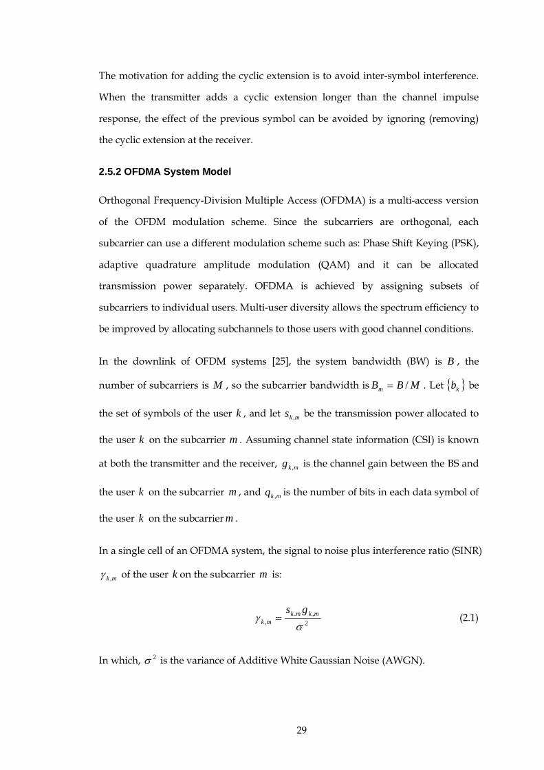
2.5.2 OFDMA System Model
Orthogonal Frequency-Division Multiple Access (OFDMA) is a multi-access version
of the OFDM modulation scheme. Since the subcarriers are orthogonal, each
subcarrier can use a different modulation scheme such as: Phase Shift Keying (PSK),
adaptive quadrature amplitude modulation (QAM) and it can be allocated
transmission power separately. OFDMA is achieved by assigning subsets of
subcarriers to individual users. Multi-user diversity allows the spectrum efficiency to
be improved by allocating subchannels to those users with good channel conditions.
In the downlink of OFDM systems [25], the system bandwidth (BW) is B , the
number of subcarriers is M , so the subcarrier bandwidth is MBBm /= . Let { }kb be
the set of symbols of the user k , and let mks , be the transmission power allocated to
the user k on the subcarrier m . Assuming channel state information (CSI) is known
at both the transmitter and the receiver, mkg , is the channel gain between the BS and
the user k on the subcarrier m , and mkq , is the number of bits in each data symbol of
the user k on the subcarrier m .
In a single cell of an OFDMA system, the signal to noise plus interference ratio (SINR)
mk ,γ of the user k on the subcarrier m is:
2
,., σ
γ mkmkmk
gs= (2.1)
In which, 2σ is the variance of Additive White Gaussian Noise (AWGN).

30
Assuming a QAM scheme is used in the OFDM system, the bit error rate (BER) of the
user k on the subchannel m can be expressed as [26]:
−
−≤
125.1
exp51
,
,
mkqmkBER
γ (2.2)
If 2, ≥mkq and dBmk 300 , ≤≤ γ , the expression (2.2) will be satisfied. For a certain
BER, the max number of sent bits in each symbol is:
Γ
+= mkmkq ,
2, 1logγ
(2.3)
in which, Γ is constant with a particular BER; this expresses the difference between
the Multiple Quadrature amplitude (M-QAM) signal and Shannon channel capacity.
In an Additive White Gaussian Noise (AWGN) channel, ( ) 5.1/5ln BER−=Γ [26].
2.5.3 Advantages of OFDMA
High Spectral Efficiency: After the IFFT operation, subcarriers can overlap partially
so the symbol transmit rate can achieve the Nyquist limitation [16]. The OFDMA
system assigns different subcarriers to different users, so users are orthogonal to each
other, and the interference between users is reduced substantially. Hence, OFDM
technology can increase the system throughput.
Simple System Implementation: Since subcarriers are orthogonal to each other, the
Discrete Fourier Transform (DFT) can be used to represent OFDM symbols. The
computational complexity of DFT is very high, ( )2nο . However, using IFFT/Fast
Fourier transform (FFT) instead of IDFT/DFT, the computational complexity of the
OFDM algorithm is reduced to ))((log2 No [16].
Anti-fading and Anti-interference: OFDMA is good against frequency-selective
fading and interference. Because OFDM divides the wideband transmission into

31
narrowband transmission on different subcarriers, each channel (subcarrier) can be
treated as a flat fading channel [16].
Flexible Resource Allocation: OFDMA can select certain subcarriers for
transmission according to channel condition, so dynamic frequency allocation can be
achieved; it can also fully make use of frequency diversity and multi-user diversity to
get optimal system performance [16].
2.6 Deployment of Fixed Relay in OFDMA Cellular Systems
Adding relay stations (RS) between the base station (BS) and the mobile stations (MS)
in OFDMA cellular systems can extend network coverage, overcome multi-path
fading and increase the capacity of the system. However, there are some important
parameters that affect overall system performance, such as the distance between the
BS and RS, and the number of relays, the number of hops, and the frequency reuse
factor.
2.6.1 Hops between BS and MS
In a relay system, traffic is transmitted over multi-hop paths. By reducing the
attenuation between the transmitter and the destination, the system performance can
be improved. Deploying a sufficient number of RSs in the whole cell and finding a
suitable route with good links via multi-hops for packets can increase the overall
capacity, and reduce the congestion happening within the cells. However, the
balance between the cost of RS deployment and the performance improvement needs
to be considered [12].
Using just two hops is an approach well-known for its simplicity with respect to
routing and resource allocation. In addition, the two-hop scheme can provide a good
tradeoff between diversity gain and repetition coding [12]. In this thesis, a two-hop
structure is used between the BS and MS.

32
2.6.2 Definition of Terms
This thesis uses the normally accepted definitions that are found in the literature:
• Direct link user is the user that communicates with the BS directly.
• Relay link user is the user that communicates with the BS via RS using two-
hops.
• Direct link is the link between BS and user.
• Relay link is the link between BS and RS (the first-hop link) and the link
between RS and MS (the second-hop link).
This normal definition of links and nodes for a relay network is shown in Figure 2.6.
BS
RS
Relay link user
Direct link userDirect link
First hop link
Second hop link
BS
RS
Relay link user
Direct link userDirect link
First hop link
Second hop link

33
MS knows that communication is routed through the RS so the frame structure
design should consider the synchronization problem of BS and RS.
The frame structure consists of downlink (DL) frame period and uplink (UL) frame
period. If the system is TDD, a time guard (TG) will be inserted between the DL
frame and the uplink (UL) frame.
The transparent frame structure in the downlink is shown in Figure 2.7 [27].
Second time subslot
BS to RS BS to Direct link user
BS silence
RS receive(The first hop link)
RS to MS(The second hop link)
Direct link user receive Relay link user receive
DL time slotFirst time subslot
MS
RS
BS
Figure 2.7 The DL transparent frame structure in relaying system
The non-transparent frame structure in the downlink is shown in Figure 2.8.
Second time subslot
BS to Direct link user
RS receive(The first hop link)
MS IdleDirect link user receiveRelay link user receive
DL time slotFirst time subslot
MS
RS
BS
RS to Relay link user
BS to RS
Figure 2.8 The DL non-transparent frame structure in relaying system
The transparent frame structure is used in this thesis. The BS schedules subchannels
in each transmission time interval (TTI). One TTI can contain one or several time
slots. In this thesis, one TTI equals one time slot, as finer scheduling interval
granularity makes better use of quickly changing channel conditions. As a relay link
is divided into the first hop link and the second hop link, a time slot is also divided

34
into the first time subslot and the second time subslot. For example, in the downlink,
the subchannels in the first time subslot are allocated to the direct link users and the
first hop of relay link users; the subchannels in the second time subslot are allocated
to the second hop of relay link users.
2.6.4 Frequency Band
In relay based cellular networks, a transparent RS uses the same carrier frequency to
communicate with nodes above and below it (BS and MS in a 2-hop network); a non-
transparent RS may use the same or different frequencies [28]. A single frequency
network with transparent RS is considered in this thesis, so the BS-RS link uses the
same frequency band as the RS-MS link.
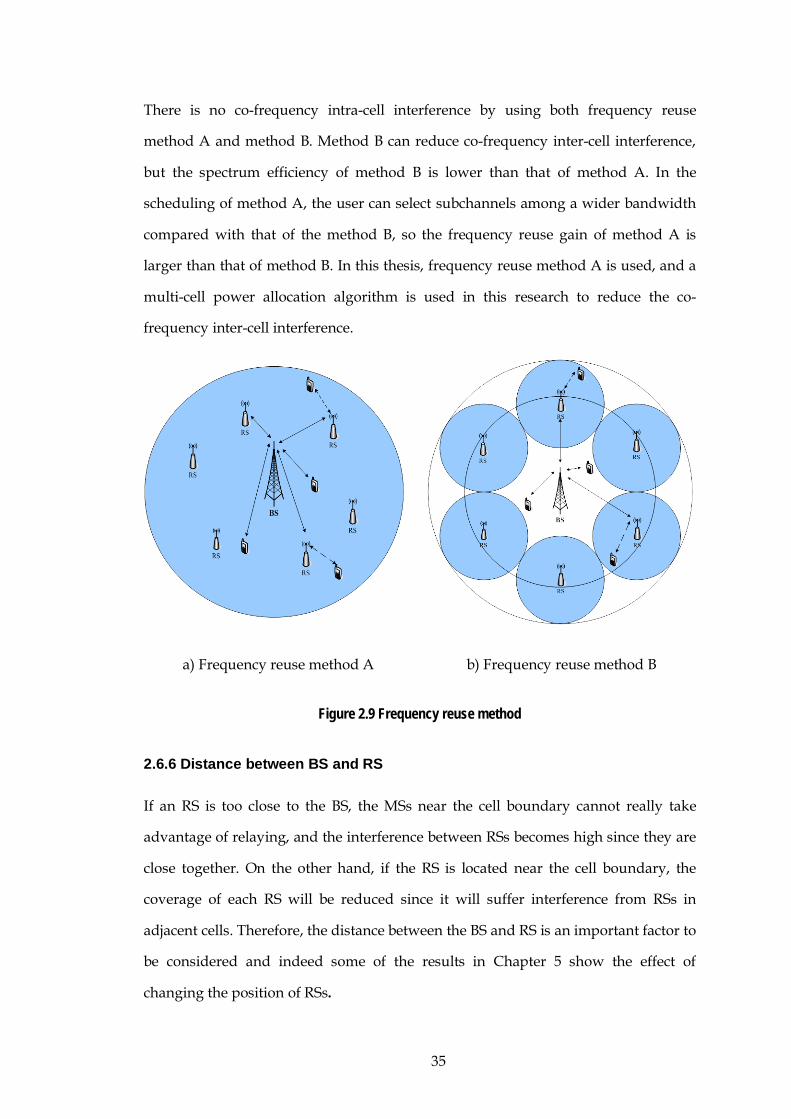
2.6.5 Frequency Reuse Method
There are two main frequency reuse methods [29]. The first method is shown in
Figure 2.9a: the frequency reuse factor (FRF) of this transmission type is one. In the
downlink, the BS transmits data to direct link users and RSs on same frequency band;
all RSs transmit data to relay link users on the second time subslot, sharing the same
frequency band as the first time subslot (TDD). Similarly, in the uplink, relay link
users transmit data to RS in the first time subslot on the whole frequency band, and
in the second time subslot, direct link users and RSs transmit data to BS using the
same frequency band as that of the first time subslot (TDD).
The second frequency reuse method is shown in Figure 2.9b, in which the whole
frequency band is divided into n sub-band for n RS and the RSs will relay data on
separate frequency bands. In the downlink, the BS transmits data to all direct link
users and RSs using the whole frequency band in the first time subslot, and each RS
transmits data to relay link users within its coverage using independent sub-bands in
the second time subslot. In the uplink, relay link users transmit data to their RS using
the sub-band of this RS in the first time subslot and the direct link user and RS
transmit data to the BS using the whole frequency band in the second time subslot.
35
There is no co-frequency intra-cell interference by using both frequency reuse
method A and method B. Method B can reduce co-frequency inter-cell interference,
but the spectrum efficiency of method B is lower than that of method A. In the
scheduling of method A, the user can select subchannels among a wider bandwidth
compared with that of the method B, so the frequency reuse gain of method A is
larger than that of method B. In this thesis, frequency reuse method A is used, and a
multi-cell power allocation algorithm is used in this research to reduce the co-
frequency inter-cell interference.
a) Frequency reuse method A b) Frequency reuse method B
Figure 2.9 Frequency reuse method
2.6.6 Distance between BS and RS
If an RS is too close to the BS, the MSs near the cell boundary cannot really take
advantage of relaying, and the interference between RSs becomes high since they are
close together. On the other hand, if the RS is located near the cell boundary, the
coverage of each RS will be reduced since it will suffer interference from RSs in
adjacent cells. Therefore, the distance between the BS and RS is an important factor to
be considered and indeed some of the results in Chapter 5 show the effect of
changing the position of RSs.

36
2.7 Summary
This chapter introduces the relevant concepts in relay networks, including the basic
concept of relay, the usage model of relay, the classification of relay, and the relevant
research in relay networks. Also, the basic concept of OFDMA is introduced and the
network configuration in relay based OFDMA networks is discussed, including the
number of hops between BS and MS, definition of terms in relay networks, frame
structure, frequency band, frequency reuse method and distance between BS and MS.

37
Chapter 3 Simulator for OFDMA Relay Networks
3.1 Overall Design of Simulation Platform
This simulation platform was built based on an existing downlink non-relay OFDMA
system level platform and all the modules are modified to produce a downlink relay
based OFDMA system level platform by the author and to add in the specific
algorithms proposed in this thesis. The simulator is designed based on IEEE 802.16j
[9][27][30], and Long Term Evolution (LTE) [31][32][33]. The main simulation
modules are listed below and the details of each module are given in section 3.3.
Initialize module: Creates network topology, initializes the position of BS, RS, and
MS, computes large scale pathloss and shadow fading.
Multi-path fading channel module: Creates multi-path fading channel, including
relay links and direct links.
CQI feedback module: Calculate the channel quality information (CQI), and feeds
back the CQI to BS. The CQI information includes: CQI of BS to RS, CQI of RS to MS,
and CQI of BS to MS.
Relay selection module: For each user, a certain RS should be selected to forward
and transmit data. Different relay selection algorithms would result in different relay
selection decisions.
Scheduling module: The subchannels in the first time subslot will be allocated to the
RSs and the direct link users; the subchannels in the second time subslot will be
allocated to the relay link users in terms of the scheduling algorithm according to the
frame structure of relaying systems [27]. Different scheduling criteria would result in
different system performance.

38
Power allocation module: Based on a particular power allocation algorithm, the BS
allocates the power to each subchannel in the first subslot, and the RS allocates the
power to each subchannel in the second subslot.
Channel capacity calculation module: Based on allocated subchannel and allocated
power of each user, each user’s CQI and data rate within one TTI is calculated.
System performance statistics module: Calculates the statistics of system
performance, including data rate, packet loss rate and packet delay.
The simulation uses time-stepping (with the time step being equal to the TTI).
The flow within the simulator is shown in Figure 3.1.

39
CQI feedback
Multipath Channel Creation
Relay Selection
Capacity Calculation
Power Allocation
Scheduling
Start
TTI End
Yes
No
NextTTI
Initialize
End
Simulation End
Yes
No
Simulation result output
NextSeedLoop
Resource Allocation
Module
Figure 3.1 Flow chart of simulator
3.2 Simulator System Parameters
A downlink relay based OFDMA system is considered here.
In the OFDMA system, every 25 continuous subcarriers compose a subchannel,
which is one frequency unit of resource allocation. One transmission timing interval
(TTI) is 1 ms, and each TTI is one time unit of resource allocation. Detailed
parameters of the downlink system are listed in Table 3.1 [31][32].

40
Table 3.1 Downlink transmission parameters
Parameter Value Transmission Bandwidth 10 MHz TTI 1 ms Subcarrier spacing 15kHz Number of subcarriers occupied 601 [-300,300] Number of subcarriers in use 600, subcarrier # 0 is not used Subchannels 24 Subcarriers/subchannels 25 (consecutive) Subchannel BW (kHz) 375
In this simulator, a typical urban macro-cell is used (defined in the 3GPP scenario
Case 2 [33]), and detailed system level simulation parameters of the macro-cell
reflecting typical values in an urban macro cell area are listed in Table 3.2; the
transmission power of the RS is a half of that of the BS, as in [34][35][36]. The channel
model refers to the IEEE 802.16j document which will be considered in Section 3.4.
Note that a wrap-around model (19 cells as centre cluster) is used [33]. There are six
RSs sited uniformly in each cell as is commonly used in the literature [36] and it is
assumed that no additional spectrum is available and, hence, all links use the same
spectrum.
The urban macro-cell scenario is chosen as that is the most likely for relay systems to
increase the system capacity whereas in rural areas it is coverage that is usually the
design consideration. However, the approach taken is generic and could be applied
in principle to any type of cell layout, including rural and suburban.

41
Table 3.2 System level simulation parameter of Macro-cell
Parameter Value Cellular Layout Hexagonal grid, 19 cell sites Inter-site distance 500 m Central Frequency/Bandwidth 2.0 GHz/10MHz Total BS TX power 20 W Total RS TX power 10 W MS power class 250 mW Minimum distance between MS and BS >= 35 meters Thermal noise density -174 dBm/Hz Penetration Losses 20 dB
Target BER 310−
Number of simulation drops 20 Simulation time per drop 1000 TTI
3.3 Module Functions and Implementation
The functions of main modules of the simulation platform are briefly explained
below.
3.3.1 Initialisation Module
Function description: This module initializes the parameters of the system, and sets up
the basic settings of the system, including the deployment of BSs, RSs and MSs, the
measurement of antenna gain, the determination of pathloss and shadow fading.

42
Start
End
19 Cells Topology Creation
RS Creation
Antenna Gain and Pathloss Calculation
Shadow Fading Creation
MS Creation
Figure 3.2 Flow chart of initial module
3.3.2 CQI Feedback Module
Function description: SINR of users on all subchannels can be calculated using (i) the
BS sending power, (ii) the user’s large scale fading, (iii) small scale (multi-path)
fading (iv) co-channel interference from other cells and (v) AWGN.
Start
Create Multipath Fading Channel
Calculate Signal Power and Interference Power
End
Calculate SINR of User on Each Subchannel
Figure 3.3 Flow chart of CQI feedback module

43
3.3.3 Resource Allocation Module
Function description: Based on the channel quality indicator (CQI) report from the
previous TTI, resource is allocated to users according to the resource allocation
algorithm. The resource here includes the choice of RS, subchannel and transmission
power.
In the downlink, BS chooses to transmit data via relay link or direct link. If it
transmits via relay, the BS needs to decide which relay will be used (the relay
selection). There are two time subslots in one TTI. In the first time subslot, under
equal power allocation, the BS allocates subchannels for relay link users and RSs; in
the second time subslot, the BS allocates subchannels for relay link users. After the
subchannels are allocated, the transmission power can be adjusted on each
subchannel. The transmission bit rate on each channel can then be calculated using
the Shannon formula.
This is the core module for the work reported in this thesis and the flow chart is
shown in Figure 3.4.
Start
Subchannel Allocation
Power Allocation
End
Capacity Calculating
Relay Selection
Figure 3.4 Flow chart of resource scheduling module

44
3.4 Channel Module
In a wireless communication system, the channel state plays an important role in
determining the system performance, and it greatly affects the quality of
communication. In order to rapidly and accurately simulate channel states, a large-
scale fading (pathloss and shadowing) model, and small scale fading (multi-path
fading) model are considered in this channel module. There are three kinds of links
in relay based cellular networks: (i) the direct link (the link between BS and MS), (ii)
the first hop link (the link between BS and RS) and (iii) the second hop link (the link
between RS and MS). An urban macro-cell scenario is used in this paper, assuming
BS and RSs are all sited above roof top (ART), and users are sited below roof top
(BRT).The small-scale fading model used here is essentially that in [30].
3.4.1 Pathloss Model
The channel model of urban macro-cell scenario uses the Type H above roof top
(ART ) to ART model in [30] to simulate the fixed relay scenario.
3.4.1.1
The pathloss scenario of BS-RS link is shown in
Pathloss between BS and RS
Figure 3.5 (Figure 2 from [29]), where
node antennas have line-of-sight (LOS) between them.
Figure 3.5 BS-RS link with LOS

45
The pathloss is determined using the COST 231 model (Appendix A in [37]) (but
excluding the rooftop-to-MS diffraction loss because the link between BS and RS is
LOS), and consists of the free-space pathloss plus the multiscreen diffraction loss
msdL .
The free space pathloss model is shown below (log denotes log to base 10)
( ) ( )kmdMHzfL cf /log20/log2044.32 ++= (dB) (3.1)
where d is distance between BS and RS, and cf is the carrier frequency.
The multiscreen diffraction loss msdL is
( ) ( ) ( )metrebMHzfkkmdkkLL cfdabshmsd log9log/log −+++= (3.2)
where b is the distance between two buildings (in metres). Furthermore,
( )bbsh hL ∆+−= 1log18 (3.3)
where roofbb hhh −=∆ is the difference between the height of the BS, bh , and that of
the building roof, roofh .
From [30], values used are: 54=ak , 30=bh m, 15=roofh m, 30=b .
The dependence of the pathloss on the distance and frequency is given by
parameters dk and fk ; here values are chosen as 18=dk and
( )1925/5.14 −+−= cf fk for a metropolitan area according to the specifications of
COST 259 [29].
The total pathloss L between BS to RS on the first hop link is

46
)(log)925/5.15.14()(1384317.51 1010 ccmsdf ffdogLLL +×++×+=+= (3.4)
3.4.1.2
BS and RS are sited above the rooftops (ART) and MSs are below the rooftops (BRT),
so there is non-line-of-sight (NLOS) between them. The pathloss is determined using
the COST 231 model
Pathloss between BS and MS
[37] which consists of the free-space pathloss fL , the
multiscreen diffraction loss msdL and the rooftop-to-street diffraction loss rtsL . The
free-space pathloss model fL and the multiscreen diffraction loss msdL expression are
the same as (3.1) and (3.2) respectively.
The rooftop-to-street diffraction loss is
0101010 )(log20log10log109.16 LhfwL mcrts +∆++−−= (3.5)
where w is the width of street (here 12=w m), and mh∆ is the height difference
between the building and the MS, the height of the user terminal is taken to be 1.6m,
so 4.136.115 =−=∆ mh m. Also from COST 231, 0L is a function of the street
orientation, which here is chosen to be 90 , so that )3590(114.040 −−=L using
the work in that reference [30].
The total pathloss L between BS to MS on the direct link is
)/(log)925/5.15.24()/(log380120.44 1010 MHzffkmd
LLLL
cc
rtsmsdf
××+++=
++= (3.6)
3.4.1.3
The pathloss between RS and MS is determined by the Cost 231 Walfisch-Ikegami
model (Appendix A in
Pathloss between RS and MS
[37]) including the free-space pathloss fL (3.1), the

47
multiscreen diffraction loss msdL (3.2), and the rooftop-to-street diffraction loss rtsL
(3.5).
The parameters are defined as follows:
20=rsh m, 15=roofh m, the height between RS and roof is 51520 =−=∆h m.
The total pathloss between RS to MS is
)/(log)925/5.15.24()/(log381.67955 1010 MHzffkmd
LLLL
cc
rtsmsf
××++×+=
++= (3.7)
3.4.2 Shadow Fading Model
The level of shadow fading is usually simulated by using a log-normal distributed
random variable [30], this refers to typical log-normal shadow fading model [30] is
used here. To simplify the shadow fading, correlation of shadowing fading is not
considered in this thesis. There is no shadow fading between BS to RS which are both
located on the rooftop, but has to be considered between BS to MS and RS to MS, in
which the standard deviation value is 8 dB under NLOS transmission [30].
3.4.3 Multi-path Fading Model
OFDM has the ability to resist multi-path effects produced by fast fading but since
this work focuses on the adaptive resource allocation scheme a fast fading channel
model should be considered in the OFDM system simulation platform.
The triple-path SUI channel model [30] is used in the simulation here. The link
between BS and RS is the SUI-3 model [30], and both the BS to MS link and RS to MS
link is the SUI-4 model [30]. The parameters used in SUI-3 and SUI-4 are given in
Table 3.3 and Table 3.4.
The code published in [37] is modified in the simulation here.

48
Table 3.3 SUI-3 Model
Tap 1 Tap 2 Tap 3 Unit Delay 0 0.4 0.9 Ms Power 0 -5 -10 dB
K factor 1 0 0 —— Doppler 0.4 0.3 0.5 Hz
Table 3.4 SUI-4 Model
Tap 1 Tap 2 Tap 3 Unit Delay 0 1.5 4.0 Ms Power 0 -4 -8 dB
K factor 0 0 0 ——
Doppler 0.2 0.15 0.25 Hz
3.5 Verification and Validation
As the credibility of simulation model is important groundwork of this thesis, the
simulation code has been debugged line by line with the help of breakpoints.
3.5.1 Verification of Relay Location and MS Distribution
The relay based multi-cell scenario is shown in Figure 3.6. Nineteen cells with wrap
around technology are used in this thesis, which meets the system design
requirement. In each cell, six RSs (blue stars) are located on the lines that connect the
cell centre to one of the six cell vertices. MSs are uniformly distributed among all the
cells. In each cell, the distribution of the MSs is different, which satisfies the user
random distribution characteristic.

49
-1 -0.5 0 0.5 1
-1
-0.5
0
0.5
1
RSMS
Figure 3.6 Distribution of MSs and RSs in multi-cell system
3.5.2 Verification of Channel States
A verification result for a large-scale channel is shown in Figure 3.7. Taking large-
scale channel fading from BS to MS for example, Figure 3.7 is the cumulative
distribution function (CDF) curve of large scale fading value (in dB). In Figure 3.7,
the channel fading value is range from -160 dB to -100dB, and it is -97 dB when the
probability value is 0.5. This result complies with the evaluation result of [38], which
can verify the large scale fading channel design.
In [38], the Figure 5 is the results of Macro urban scenario, in which, the BS transmission power is 40 W, BS max antenna gain is 17 dB, BS sector antenna gain is 20 dB. In this thesis, the BS transmission power is 20 W, BS antenna gain is 0 dB, BS sector antenna gain 0 dB (omni antenna pattern). So the large scale fading in this thesis is 40dB less than that of [38].

50
-180 -160 -140 -120 -100 -80 -60 0
0.1
0.2
0.3
0.4
0.5
0.6
0.7
0.8
0.9
1
Large scale fading (dB)
F(x)
Empirical CDF
BS-MS
Figure 3.7 Verification of large scale channel fading between BS and MS
Verification of multipath fading channel is shown in Figure 3.8. The each tap of the
envelope of the multipath fading is a Rayleigh-distributed with mean σπ2
and
variance 2
24 σπ− (the normalised transmission power is used in multipath fading,
so 12 2 =σ [Andrea Goldsmith, WIRELESS COMMUNICATIONS]). In Figure 3.8,
the CDF curve of the envelope of multipath fading (one tap) is shown, with mean
0.8786 and variance 0.2124 by statistic. This means that the result of the multipath
fading simulation complies with the Rayleigh-distributed.

51
0 0.5 1 1.5 2 2.5 3 3.50
0.2
0.4
0.6
0.8
1
x
F(x)
Empirical CDF
mean: 0.8786median: 0.8720 std: 0.4690
Figure 3.8 Verification of fast fading channel
3.5.3 Verification of Number of Drops
In the simulation, a random “drop” is the term used to describe the random placing
of users in the scenario – not the disconnection of call in progress.
For each drop, the distribution of users obeys the specified distribution (here
uniform distribution), but the actual location of MSs will change drop to drop. From
a theoretical view, the bigger the number of drops, the more accurately the user
distribution will approach the ergodic uniform distribution. From the simulation
point of view, the bigger the number of drops, the longer the simulation time will be.
Therefore, a reasonable number of drops need to be chosen. In Figure 3.9, system
throughput is compared with different number of drops. In the simulation, there are
20 users within each cell, and the system parameters are as listed in Table 3.1 and
Table 3.2; the subchannel allocation algorithm used here is the partial proportional
fairness scheduling algorithm (PPF) in [36] and the relay selection algorithm is the large-
scale relay selection algorithm in [40]. In Figure 3.9, the blue histogram shows the
average system throughput when the number of drops is 100, and the red histogram

52
shows the average system throughput when the number of drops is 20. Simulation
results show that the percentage difference of system throughput is within 5%.
Moreover, the simulation results are more concerned about comparison between
different algorithms and less on the absolute value of algorithm performance.
Therefore, 20 drops is taken as a reasonable tradeoff between accuracy and
simulation time and is used throughout this thesis.
1:20 21:40 41:60 61:80 81:1000
0.5
1
1.5
2
2.5
3
3.5
4
4.5
5
5.5x 10
7
Number of drops
Ave
rage
thro
ughp
ut
Average of 20 dropsAverage of 100 drops
4.5%2.2% -0.2% -4.2% -2.3%
Figure 3.9 System throughput vs. number of drops
The simulation result is compared with the results of other relevant studies in [36]
which are accurate to the same order of magnitude. In [36], the central frequency is
5 GHz and system bandwidth is 1 MHz; when the number of users is 10, the spectral
efficiency of the PPF algorithm proposed in [36] is about 4.5 bps/Hz. The PPF
algorithm is implemented in the simulator here for verification. In this thesis, the
central frequency is 2 GHz and system bandwidth is 10 MHz and when the number
of users is 10, the spectral efficiency of the PPF algorithm proposed in [36] is about
4.4 bps/Hz (can be calculated from Figure 3.10). It can be concluded that the
simulation results are of the same order of magnitude.

53
10 15 20 25 30 35 40 45 500
1
2
3
4
5
6
7
8x 10
7
Number of users in each cell
Ave
rage
thro
ughp
ut (b
ps)
PPF
Figure 3.10 System throughput vs. number of users
3.6 Summary
A description of the overall design of the simulation platform and system parameters
is given in the first part of this chapter, together with the system parameters. This is
followed by a more detailed explanation of the most important modules. The
channel model is introduced in the end of this chapter including pathloss model,
shadow fading model and fast fading model.

54
Chapter 4 Radio Resource Allocation in OFDMA Relay
Networks
4.1 Introduction to Radio Resource Management
The radio resource in wireless networks includes: transmission power, time-domain
resource, frequency-domain resource and spatial-domain resource. The object of
radio resource management is i) to improve system validity and reliability given the
finite radio resource available, ii) to satisfy different quality of service (QoS)
requirements for different types of application from users, and iii) to maximize the
radio resource efficiency. The basic idea of radio resource management is that, as the
channel state varies with the changing of channel fading and interference, the radio
resource in the wireless system can be allocated flexibly and adjusted dynamically to
meet the QoS requirements of users, and the system throughput and spectrum
efficiency can be improved.
Radio resource management can be classified into three main parts: radio resource
allocation, mobility management and spectrum management. Radio resource
allocation focuses on allocating the radio resource to different users. When a user is
moving, mobility management too becomes necessary. Spectrum management is
about how best to divide up the available bandwidth from the whole system point of
view.
Radio resource allocation is important for increasing wireless network capacity.
There are three main issues which need to be solved in wireless resource allocation:
the first, which wireless access point will be connected for wireless terminal; the
second, how the system allocates subchannels to users; the third, what power level
should be used in the transmitter.
The first issue is solved by access control and load control. Access control decides
whether to accept the new access request and which access point provides the

55
wireless connection. Traffic load control can avoid the system load being too heavy,
so causing the channel condition to deteriorate and changing the service
characteristics.
A good channel allocation mechanism can solve the second issue in wireless resource
allocation, improving the system throughput and user performance by allocating
channel resources in the best possible way. In TDMA systems, the channel resource
is a time slot; in FDMA systems, it is a frequency subchannel; in CDMA systems it is
a code; and in OFDMA systems, the channel resource is a time-frequency two-
dimensional block, which is defined as subchannel [41].
Packet scheduling determines the output order of the packets in the traffic buffer. For
single-carrier systems, the channel is allocated to users if the packets of that user are
being scheduled, i.e. scheduling has the same function as channel allocation in single
carrier channel systems. For multi-carrier systems (OFDMA systems), during one
scheduling interval, the packets can be transmitted in more than one subchannel. So,
after packet scheduling, the subchannel needs to be allocated. Currently, most
algorithms consider the packet scheduling and subchannel allocation jointly.
Power control (or power allocation) is used to solve the third issue. In wireless
networks, transmission power is not only relevant to the performance of the target
receiver, but also affects the performance of other receivers using the same
subchannel. In 3G systems, power control is used to reduce the co-frequency
interference within the cell, and to mitigate far-near effect [42].
In OFDMA systems, power control can be used to compensate propagation loss and
shadow fading [43]. Moreover, power allocation should be considered to compensate
the fast fading. So, compared with power control, the power allocation interval is
short and the granularity of power allocation is finer. To guarantee both the
performance requirement for a particular user as well as for the whole system, power
allocation and subchannel allocation are usually considered jointly in each
subchannel in every scheduling interval [44]. Besides, since the frequency reuse

56
factor is one in OFDMA systems, power allocation is one of the important methods
to minimize the effect of inter-cell interference [45][46].
As mentioned in Section 2.4, resource management is a key factor in relay based
cellular systems and different aspects have been researched. The resource allocation
scheme devised by the author and presented in Section 5.3 captures relay selection
and channel allocation tasks. However, before considering that novel work, it is
necessary to discuss previous research on relay selection, channel allocation and
power allocation.
4.2 Relay Selection
As discussed in Section 2.6.1, two-hop relaying is a good design choice for the
tradeoff between performance gain and system complexity. In this case the routing
problem is simplified into a relay selection problem, which can simplify the protocol
design and minimize the communication overhead significantly compared with
more complex structures (such as mesh network).
Relay selection aims at improving the data rate transmitted from the source to the
destination by forwarding traffic via a suitable RS with spare capacity that is
experiencing a more favourable channel condition. While it might appear at first
sight that relay selection (routing) is similar to that in ad hoc networks, there are
significant differences [12]:
• Small number of hops compared with a full scale ad-hoc network.
• Central processing: in multi-hop cellular networks, there is an infrastructure
unlike ad-hoc networks; also the location information and flow direction in
both uplink and downlink are available, especially for the case where fixed-
relays are used.
• Fewer energy constraints: in contrast with the case of ad-hoc networks,
especially where fixed relays are used, the power constraints and energy
efficiency are not so critical in relay networks.
57
Various selection schemes for the relay and relay channel, from random to smart
selection, with and without power control, are considered in [40]. It is observed that
with the proper selection of relay, relay channel, and relay power, a significant
enhancement in high-data-rate coverage can be attained through two-hop mobile
relaying.
In an infrastructure-based network with fixed relays, the selection of relays is more
or less predefined. The relay selection approaches based on centrally controlled
methods can be used for selecting the RS for every MS in each cell, and various
selection criteria can be used for designing the relay selection method. Distance
based relay selection algorithms [40][47] and pathloss based relay selection
algorithms [40][48] have been proposed; a transmission power-based relay selection
algorithm is proposed in [49] and a congestion-based relay selection algorithm is
studied in [50].
[51] considers the relay selection problem in a basic amplify-forwarding relay
scenario that has one source and two destinations, so the problem is required to
decide which node will be used as RS. The proposed schemes in [51] are the (i)
classical round robin and (ii) a channel-based scheduling policy that requires a
partial feedback from the channel. This scheme is implemented in a centralized and a
distributed version. With a centralized strategy, routing is performed in a central
controller, which normally possesses powerful processing capabilities so that
sophisticated routing algorithms may be used. While this may optimize the system
performance, it does require a lot of information to be obtained from the distributed
network nodes and passed to the central controller; this leads to a significant
message-passing overhead. With the distributed version, all network nodes from the
source to the destination jointly perform route determination. This approach can be
used without a central controller but the performance is normally limited by the
knowledge of the network status within the distributed nodes [51].

58
In [52], relay selection is investigated in relay systems in which user terminals act as
relays. Relay selection with mobile relays is more complicated than fixed relays as
the topology of mobile relays is not fixed. However, this thesis considers only fixed
relays so mobile relays are not considered further.
4.3 Channel Allocation
In [53], a distributed scheduling algorithm is proposed for a downlink relay network,
in which MSs act as mobile relays. The authors use a scalable factor-graph-based soft
information-passing algorithm to schedule simultaneous data transmissions in a
distributed way. Not only dynamic routing paths for data packets are obtained, but
also direct data collisions among simultaneously transmitted data packets are
avoided.
The scheduling problem in a cooperative relay system is considered in [54], in which
the system diversity gain is achieved by amplify and forwarding cooperative relays
and the multi-user gain is obtained from adaptive channel scheduling.
The authors in [55] propose a radio resource allocation in fixed relay systems in
which the optimization objective is maximizing system throughput. It is proved that
this optimization problem is a NP-hard problem, so a heuristic algorithm is proposed
in [55], which is called combined resource allocation, including routing, scheduling and
relay load balancing. The scheduling scheme can adaptively handle different
transmission modes (direct link mode or multi-hop link mode).
Traditionally, the channel variation in wireless networks is considered as a negative
factor for reliable communication, and methods such as time interleaving, power
control and multiple antennas are used to reduce its impact. On the other hand,
opportunistic scheduling is designed to exploit the variation in channel conditions to
improve spectrum efficiency by adding an additional degree of freedom to the
system: time domain diversity, also called multi-user diversity. It improves spectrum
efficiency, especially for delay-tolerant data transmissions [56].

59
In an opportunistic scheduling scheme, the user that has a good channel gain will
have a greater opportunity to occupy this channel, so the resource can be used
efficiently and the system performance improved. The proportional fairness (PF)
scheduling algorithm used in CDMA High Data Rate (HDR) system is an
opportunistic scheduling scheme [57]. The PF algorithm not only considers the
instantaneous achievable data rate in each TTI, but also considers the average data
rate of a user, which gives a good tradoff between system throughput and user
fairness.
In [58] traffic-aided smooth admission control and relay aided opportunistic
scheduling (RAOS) are proposed in TDMA relay systems. First, the transmission
mode of the user (direct-link or two-hop link) is decided, and then the priority of
each user in each time subslot is calculated. The scheduler chooses the user k with the
highest priority. If the user is using a two-hop link, the BS sends data to the user k via
the selected relay station r(k), otherwise it sends data directly.
A partial proportional fairness scheduling (PPF) scheme is proposed in [36] for relay
based OFDMA/TDD cellular systems, the traditional proportional fairness algorithm
being used for the resource allocation in the second time subslot. Both direct link
users and two-hop relay link users have the opportunity to be allocated in the second
time subslot. In the first time subslot, RS has a priority to choose the first hop
subchannels. The priority of each RS is decided by the ratio of second-hop link
achieved throughput and first-hop link achieved throughput. The RS with highest
priority chooses the subchannel which has the biggest gain among all the
subchannels as the first-hop channel. The resource allocation to the first-hop link via
each fixed RS will end when the first-hop data rates and the aggregate second-hop
data rates reach a balance. The left-over resource units of the first-hop link will be
assigned to direct link users on the basis of the proportional fairness principle.
[59] aims to maximise the system capacity; the optimal source/relay/subchannel
allocation problem is formulated as a binary integer programming problem. The
60
problem is then tackled using a graph theoretical approach by transforming it into a
linear optimal distribution problem in a directed graph. However, the complexity of
this algorithm is very high and so is not suitable for real-time multi-hop systems. In
[60], the resource allocation between the BS and RSs in OFDMA relay systems is not
considered by assuming that the BS and RSs can communicate reliably through
dedicated frequency bands; instead a fast heuristic algorithm is studied as a joint
optimization algorithm of relay selection and subchannel allocation. In that paper,
the first step is to sort a set of subchannel gains in descending order and assign
subchannels to each user according to the sorted subchannel order. If a user receives
a certain number of subchannels, subchannel allocation to that user is stopped and
then the remaining subchannels are assigned to the user who has the best channel
gain for those subchannels.
4.4 Power Allocation
Power allocation in a relay system can be classified into two kinds of problem in
terms of constraint conditions. One is joint power constraint on BS and RS [61][62][63]
[64] (i.e. the sum of the power constraint of BS and RS is a constant) and the other is
BS and RS having separate power constraints Error! Reference source not found..
In [61], an optimal power allocation method to minimize the outage probability of a
Rayleigh fading channel is presented. Optimal power allocation to maximize the
system capacity is proposed for regenerative and non-regenerative relaying schemes
in [62] respectively. However, in [61][62][63] the system considered is not OFDM so
the first hop link and the second hop link use the same channel.
The problem of power allocation in OFDM relay systems is studied in [64][65]. In [64]
cooperative non-regenerative relays are considered; the authors give an equivalent
channel gain model for those cooperative subcarrier pairs and the optimal power
allocation problem is divided into two parts, one considers the total power allocation
on the cooperative subcarrier pairs and the other considers the power allocation

61
between the selected cooperative subcarrier pairs using the power water-filling
approach.
In [65], power allocation over the frequency subchannels of one source/destination
pair and one non-regenerative relay is studied to maximize the instantaneous data
rate of the link. It is assumed that source and relay have their own separate
transmission power constraints and the second hop link uses the same subcarrier as
the first hop link. Optimal power allocation algorithm at the relay (or source) is used
with an equal source (or relay) power allocation. Then, alternating iterative
optimization of relay and source power allocation is proposed, where the output of
the previous optimization (relay or source) is the input of the other (source or relay).
The studies of power allocation in [64] are based on the assumptions that one
subcarrier on the first hop link and one subcarrier on the second hop link make up a
subcarrier pair, i.e. the subcarriers of the two hop links correspond to each other, but
this situation only exists in non-regenerative OFDM relay channels: with a
regenerative relay channel, these kinds of subcarrier pairs do not exist.
4.5 Summary
The radio resource allocation in relay networks is introduced in this chapter. The
basic concept and content of resource management is introduced first, and then the
relevant work of relay selection, channel allocation and power allocation is
considered.

62
Chapter 5 Fair Subchannel Allocation and Relay
Selection
5.1 Introduction
The problem of fair resource allocation is more challenging in relay based cellular
systems, for there are two kinds of users: direct link users and relay link users.
Fairness issues include those (i) between relay link user and direct link user, (ii)
among relay link users and (iii) among direct link users. To solve this problem, a
two-hop proportional fairness algorithm is proposed which can give a tradeoff
between system throughput and user fairness.
The conventional algorithms [40][47] are only based on the pathloss or distance
conditions of individual users, do not consider the load of the RS, and cannot tackle
the fairness problem in terms of RS load condition, especially when users are not
distributed uniformly. So in this chapter a load based relay selection algorithm is
proposed, which takes into account the traffic load condition (bandwidth
requirement) of relay link users and direct link users, and improves the fairness of
resource allocation for OFDMA based relay systems.
5.2 System Model
5.2.1 System Parameters
In relay based OFDMA systems, the system bandwidth is B , the number of
subcarriers is C , and the access method is OFDMA. The number of RSs is R . As
explained earlier, to balance system complexity and system performance, the number
of hops is two. In practical OFDMA systems, a group of consecutive subcarriers with
similar fast fading can make up a subchannel and each subchannel can be used as a
resource scheduling unit instead of using subcarriers [16]. In this way, the control
signal overhead can be reduced, and the algorithm complexity is decreased, but the
system performance is unaffected. In the system model here, S consecutive

63
subcarriers are grouped together as a subchannel, the number of subchannels M is
SC and the bandwidth of each subchannel is MB .
In each cell, the BS chooses one communication mode (direct link or relay link) for
each MS. If the communication mode is relay link, the BS chooses one RS for each
relay link user. k is the index of a MS in each cell. The direct link user is dk and the
set of direct link users is DK . The relay link user k served by the RS r is denoted as
rk , the set of relay link users is RK , and the set of users served by the RS r is
expressed as rRK . The RS serving the user k is kr .
5.2.2 Channel Capacity
The term dkma is used to denote whether the subchannel m is allocated to the direct
link user dk ; 1=dkma indicates it is allocated and 0=dk
ma shows that it is not. In a
similar way rma represents the allocation of the subchannel m to the RS r . Similarly,
for the second hop link rkmb denotes whether the subchannel m is allocated to the
user k via the RS r , in which rk is the user k served by the RS r .
According to the Shannon formula, the capacity of the direct link user dk on the
subchannel m in the first time subslot is:
Γ+= 2
1,1,21, 1log
σ
dd
d
km
km
mkm
pgBc (5.1)
The capacity of the RS r on the subchannel m in the first time subslot is:
Γ+= 2
1,1,21, 1log
σ
rm
rm
mrm
pgBc (5.2)
The capacity of the user rk on the subchannel m in the second time subslot is:
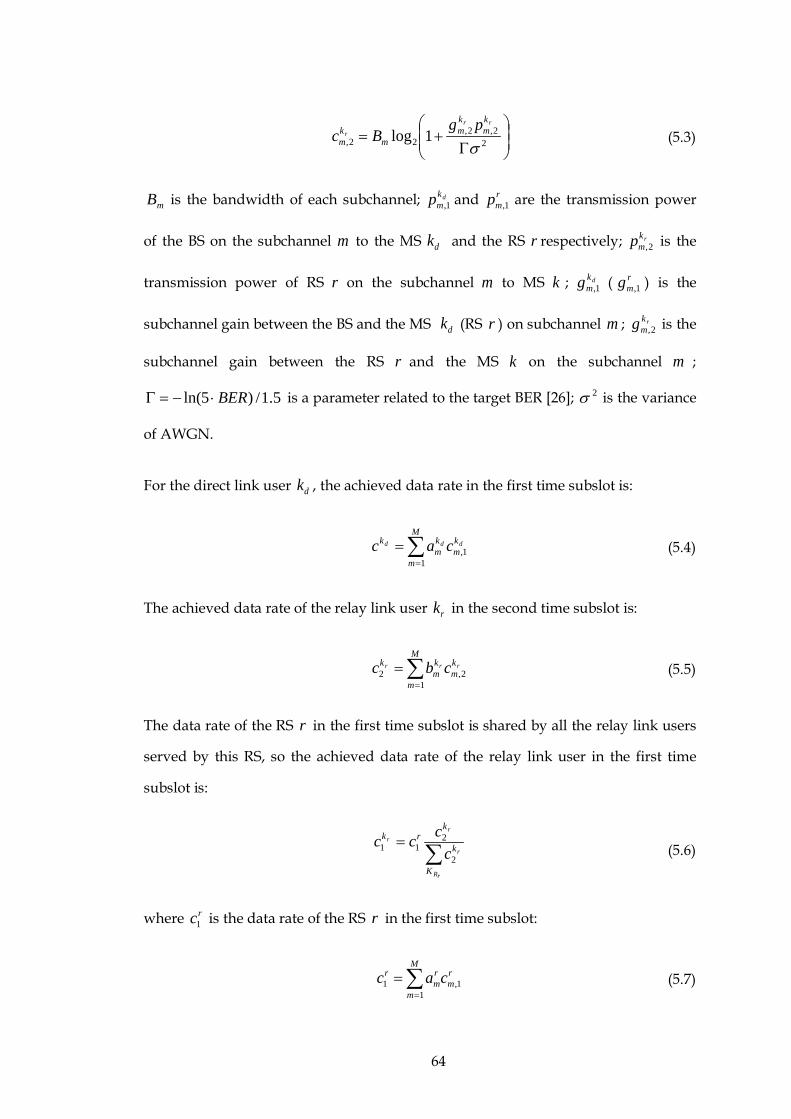
64
Γ+= 2
2,2,22, 1log
σ
rr
r
km
km
mkm
pgBc (5.3)
mB is the bandwidth of each subchannel; dkmp 1, and r
mp 1, are the transmission power
of the BS on the subchannel m to the MS dk and the RS r respectively; rkmp 2, is the
transmission power of RS r on the subchannel m to MS k ; dkmg 1, ( r
mg 1, ) is the
subchannel gain between the BS and the MS dk (RS r ) on subchannel m ; rkmg 2, is the
subchannel gain between the RS r and the MS k on the subchannel m ;
5.1/)5ln( BER⋅−=Γ is a parameter related to the target BER [26]; 2σ is the variance
of AWGN.
For the direct link user dk , the achieved data rate in the first time subslot is:
∑=
=M
m
km
km
k ddd cac1
1, (5.4)
The achieved data rate of the relay link user rk in the second time subslot is:
∑=
=M
m
km
km
k rrr cbc1
2,2 (5.5)
The data rate of the RS r in the first time subslot is shared by all the relay link users
served by this RS, so the achieved data rate of the relay link user in the first time
subslot is:
∑=
rR
r
rr
K
k
krk
cccc
2
211 (5.6)
where rc1 is the data rate of the RS r in the first time subslot:
∑=
=M
m
rm
rm
r cac1
1,1 (5.7)

65
The available data rate of the relay link user rk is determined by the minimum
capacity of the first time subslot and that of the second time subslot, which can be
expressed as:
{ }rrr kkk ccc 21 ,min= (5.8)
5.2.3 Optimization Problem
In order to consider proportional fairness across two hop links, the optimization
problem is formulated as:
) { }
)
)
)
)
=
=+
≤
≤+
∈∀=
∑ ∑
∑∑
∑∑
∑∑ ∑∑
∑
= ∈
=∈
= =
= = = =
=
15
14
3
2
,...2,1,, 1
..
max
1
1
1 12,
1 1 1 11,1,
1
R
r Kk
km
R
r
rm
Kk
km
RS
M
m
K
k
km
km
BS
M
m
K
k
M
m
K
k
rm
rm
km
km
ji
K
k
k
rR
r
D
r
rr
dd
b
aa
Ppb
Ppapa
Kjicc
ts
c
(5.9)
There are five constraint conditions of the optimal target above:
1) is the requirement of data rate fairness between users, i.e. all the users achieve the
same data rate in each scheduling interval;
2) shows the constraint on the total power of the BS;
3) shows the constraint on the total power of the RS;
4) expresses that one subchannel can only be allocated to one station (RS or direct
link user) in the first time subslot;
5) expresses that one subchannel can only be allocated to one relay link user in the
second time subslot.

66
This problem cannot be solved to yield an optimal solution directly, since it is not a
convex optimization problem, so a heuristic method to get a suboptimal solution is
used. To simplify this problem, the first constraint condition is relaxed. Long-term
fairness is pursued as a constraint condition instead of aiming for short term fairness
in each scheduling interval.
5.3 Two-Hop Proportional Fairness Algorithm
In a conventional OFDMA wireless system (no relay), the PF algorithm [6] achieves
the best tradeoff between system throughput and user fairness. However, the PF
algorithm cannot be applied directly in two-hop relaying systems since the direct
link and relay link are present simultaneously: a fair allocation problem in both the
two time subslots needs to be considered.
In this thesis, a new algorithm, called “two-hop proportional fairness” (THPF)
scheduling algorithm, is proposed to allocate the subchannels in both time subslots
with a fair subchannel allocation, in which subchannels are allocated to relay link
users fairly in the second time subslot and subchannels are allocated fairly to RSs and
direct link users in the first time subslot as well. The average data rate of the RS is
defined as the average data rate of all relay link users served by this RS, and a match
factor is proposed considering the capacity match issue between the first link and the
second link for each RS.
5.3.1 Algorithm Description
The subchannel allocation in the second time subslot is considered first. The priority
of the relay link user rk on the subchannel m in the second time subslot is defined as
the ratio of the instantaneous data rate of the user rk in the current TTI to the
average data rate of the user rk achieved in the previous TTIs. The priority of the
relay link user rk on the subchannel m is expressed as:

67
r
r
rk
kmk
m cc
q 2,2, = (5.10)
where rkc is the time average data rate of the user rk .
Each subchannel is allocated to the relay link user who has the highest priority on
this subchannel, i.e.
( ) r
Rr
km
Kkr qmk 2,* maxarg
∈= (5.11)
The subchannel m which is allocated to the user rk can be represented as rkm and
*rk
mb will be set to one.
After the subchannels have been allocated in the second time subslot, the
instantaneous data rate of the RS r on the second time subslot is:
∑∈
=rRr
r
Kk
kr cc 22 (5.12)
Next, the BS allocates subchannels to either RSs or to the direct link users in the first
time subslot as described in the following steps. The priority of a direct link user can
be expressed as:
d
d
dk
kmk
m cc
q 1,1, = (5.13)
Since the RS forwards the data received from the BS to the relay link users, the
average data rate of the RS r is represented by the mean of all time average data rate
of all the relay link users served by the RS r :
∑∈
=rRr
r
rKk
k
R
r cK
c 1 (5.14)
in which, rRK stands the number of relay link users in the set of
rRK .

68
Meanwhile, in order to fully exploit the channel capacity in the second time subslot,
the matching problem between achieved data rate in the two time subslots of each RS
needs to be considered, a match factor rβ being defined to modify the priority
function of proportional fairness.
rrr cc 12=β (5.15)
The priority function of the RS r on the subchannel m can be formulated as:
r
rmrr
m cc
q 1,1, β= (5.16)
The priority of direct link user and each RS on each subchannel is calculated by (5.13)
and (5.16), and each subchannel is assigned to the node (RS or direct link user) which
has the highest priority. For example, for the subchannel m , let dd km
km qq 1,ˆ
1, max= ,
rm
rm qq 1,ˆ
1, max= . If rm
km qq d ˆ
1,ˆ
1, > , then the subchannel m is assigned to the direct link
user dk̂ , i.e., 1ˆ=dk
ma . If rm
km qq d ˆ
1,ˆ
1, ≤ , the subchannel m is assigned to the RS r̂ , 1ˆ =rma ,
and rc ˆ1 is updated according to (5.7).
If 1ˆ ≤rβ , the RS r̂ would be excluded from the candidate RSs for the subchannels
allocation.
The achieved data rate of direct link users and relay link users during this scheduling
interval (TTI) will be updated according to (5.4) to (5.8) respectively. Lastly, the
average data rate of each user will be calculated by the exponential weighed average
data rate function [36][57]:
( ) ( ) ( ) ( )tctctc kkk ⋅+−⋅−= ρρ 11 (5.17)
where ρ is the exponential weighed factor of the average data rate function.

69
5.3.2 Algorithm Procedure
The THPF algorithm procedure is as follows:
Step1: Initialization at the beginning of each scheduling interval:
0=dkma , 0=r
ma , 0=rkmb , 0=rc , 0=dkc , 01 =rkc , 02 =rkc , mrk ,,∀
Step2: Subchannel allocation in the second time subslot:
For m=1: M
( ) r
Rr
km
Kkr qmk 2,* maxarg
∈= and 1
*
=rkmb
End
Step3: Calculate rkc1 , rkc2 , rβ , dkmq 1, , r
mq 1, .
Step 4: Subchannel allocation in the first time subslot:
For m=1: M
dd km
km qq 1,ˆ
1, max= , rm
rm qq 1,ˆ
1, max=
If rm
km qq d ˆ
1,ˆ
1, >
1ˆ=dk
ma
Else 1ˆ =rma
End
Update rc ˆ1 , rβ , r
mq ˆ1,
If 1 r̂ ≤β , the RS r̂ can’t compete for the remains of the subchannels
End

70
End
Step 5: Update , .
5.3.3 Performance Simulation and Analysis
A single-cell relay OFDMA cellular scenario is considered with six RSs uniformly
located on the line that connects the cell centre to one of the six cell vertices, as
shown in Figure 5.1. In the cell, MSs are distributed uniformly. A MS can either
connect to the BS directly, or via an RS. The relay selection scheme depends on the
pathloss [40] in this section.
Figure 5.1 Layout of single cell relay based OFDMA network
The simulation parameters of the DF relay based OFDMA network shown
previously in Table 3.1, Table 3.2 are used. It is assumed that the buffer of each RS is
sufficiently large so that in each time slot, all the data received from the BS in the first
time subslot, can be forwarded directly to the MS by the RS without considering any
data buffer size restriction.
Max Carrier to Interference Ratio (Max C/I) [36] and Round-Robin (RR) [36] are the
traditional scheduling algorithms in wireless systems. These two algorithms are

71
modified by the author to make them suitable for OFDMA relay systems and to
allow them to be compared with THPF.
Max C/I is an opportunistic algorithm that always allocates the subchannels to users
who have a good channel state. For OFDMA relay systems, in the first time subslot,
each subchannel is allocated to the node (the direct link user or the RS) with the
maximum SINR; in the second time subslot, each subchannel is allocated to the relay
link user with the maximum SINR. In this way, a high system throughput will be
obtained by Max C/I scheduling and the system resources are fully utilized.
However, those users with bad channel conditions will suffer unfairness.
RR algorithm is fair and simple when the channel conditions remain approximately
constant. However, in a fast fading channel, the RR algorithm has a low spectral
efficiency since users are scheduled in order without considering the channel
condition. In OFDMA relay systems, the RR can be modified to schedule users over
two time subslots. In the second time subslot, each subchannel is allocated to the
relay link users one by one until all the subchannels are allocated. In the first time
subslot, each subchannel is allocated to the RSs first and then the rest of the
subchannels are allocated to the direct link users in order.
In [36], a Partial Proportional Fairness (PPF) algorithm which adopts the PF
algorithm for the subchannel allocation in the second time subslot was proposed.
However, the PPF gives an absolute priority to the RS when assigning the first time
subslot subchannels, considering neither the fairness between RSs nor the fairness
between RSs and direct link users. Since the PPF algorithm is also a fair scheduling
algorithm for relay based OFDMA systems, PPF is used for comparison with the
THPF algorithm for further performance analysis. Note that in the PPF algorithm
described in [36], direct link users can be allocated subchannels in the second time
subslot; however, for better comparison with the THPF with the same frame
structure, the original PPF algorithm was modified by the author of this thesis so that

72
direct link users can only use the first time subslot for matching the frame structure
shown in Figure 2.7.
The transmission power on BS or RS is assumed to be allocated on subcarriers
uniformly; this is called equal power allocation.
In this part of the research on scheduling algorithms, the system throughput and the
user fairness are examined under equal power allocation, comparing the RR, Max
C/I, PPF and THPF approaches.
The system average throughput is the sum of average throughput across all users.
The Raj Jain fairness index [60] is adopted in this paper to measure the fairness
among users.
The Raj Jain fairness index is defined as
( )∑
∑
=
=
= K
kk
K
kk
CK
CF
1
2
2
1
~
~
(5.18)
The most fair scheduling scheme is when the average data rate of each user is equal
to others, where 1=F represents the maximum fairness – lower values are less fair.
K is the total number of users. kC~ is the time average throughput of the user k
during the simulation time.
The position of the RSs will affect the transmission mode selection and RS selection
of each user, so it is necessary to compare the system performance between Max C/I,
RR, PPF, and THPF with different RS positions (defined in terms of D , the radius of
the cell, 0.5 D , for example, meaning that the RS is 0.5 D away from the BS).
Figure 5.2 and Figure 5.3 show the system throughput and user fairness between
Max C/I, RR, PPF, and THPF against different RS normalized distance, which is
defined as the ratio of the distance between the RS and the BS to cell radius D .

73
From the simulation result of Figure 5.2 and Figure 5.3, a good system throughput
and fairness performance for these scheduling algorithms is achieved when the RS is
between 0.5 D and 0.6 D away from the BS. Thus, in the following simulation the
performance of these three algorithms is compared when the RS is located at 0.5 D
away from the BS.
From Figure 5.2, the maximum system average throughput is obtained by Max C/I
while RR has the minimum system average throughput. However, Max C/I has the
lowest fairness index while the THPF algorithm has the highest fairness index as
shown in Figure 5.3. From these figures it can be seen that the THPF algorithm offers
a good tradeoff between system throughput and fairness.
0.2 0.3 0.4 0.5 0.6 0.7 0.80
1
2
3
4
5
6
7
8x 10
7
RS nomalized distance
Ave
rage
thro
ughp
ut (b
ps)
MCIPPFTHPFRR
Figure 5.2 System throughput vs. RS normalized distance

74
0.2 0.3 0.4 0.5 0.6 0.7 0.80
0.1
0.2
0.3
0.4
0.5
0.6
0.7
0.8
0.9
1
RS nomalized distance
Fairn
ess
inde
x
MCIPPFRRTHPF
Figure 5.3 Fairness index vs. RS normalized distance
Figure 5.4 and Figure 5.5 show the system throughput and user fairness comparison
with different numbers of users.
From the simulation results Figure 5.2-Figure 5.5, it can be seen that compared with
PPF, the THPF achieves greater fairness in user data rate allocation in spite of having
only a slightly lower throughput. For example, if the RS is located at 0.5 D away
from the BS, the throughput of THPF is only 4% lower than that of PPF. However,
the fairness of THPF is 20% higher than that of PPF.
For the Max C/I and THPF algorithms, it can be concluded that system throughput
improves as the number of users increases, as shown in Figure 5.4. The reason is that
Max C/I algorithm only considers the channel conditions of users to gain maximum
multi-user diversity; therefore, as the number of users increases, the system
throughput increases but the fairness decreases (as in Figure 5.5). The THPF
algorithm and the PPF algorithm consider both system throughput and fairness so
the throughput also increases with the number of users. For the RR algorithm, the
system throughput does not change with the number of users. When the number of

75
users is small, the fairness of RR is the best of all (because there is then enough
capacity to divide fairly between the few users), but then deteriorates as the number
of users increases.
10 15 20 25 30 35 40 45 500
1
2
3
4
5
6
7
8x 10
7
Number of users in each cell
Ave
rage
thro
ughp
ut (b
ps)
MCIPPFTHPFRR
Figure 5.4 System throughput vs. number of users
10 20 30 40 500
0.1
0.2
0.3
0.4
0.5
0.6
0.7
0.8
0.9
1
Number of users in each cell
Fairn
ess
inde
x
MCIPPFRRTHPF
Figure 5.5 Fairness index vs. number of users

76
The average throughput of PPF is higher than THPF because the PPF algorithm only
aims to make full use of the system spectral diversity gain but does not consider
fairness in the first time subslot. However, the average throughput of THPF is almost
96% of that achieved by PPF and the fairness of THPF is much better than PPF, as
shown in Figure 5.4 and Figure 5.5.
In Figure 5.2-Figure 5.5, the performance of the Round Robin, Max C/I, PPF and
THPF algorithms are compared with different RS position and different number of
users. From the simulation results, it can be seen that THPF can achieve a good
tradeoff between system throughput and fairness.
5.4 Load Based Relay Selection Algorithm
The existing relay selection algorithms (such as: distance based relay selection and
pathloss based relay selection) have the advantage of being very simple for relay
based OFDMA systems. However, these algorithms decide which transmission mode
(direct link mode or relay link mode) will be used and which RS is to be chosen only
based on the pathloss or distance conditions of an individual user. For example, in a
hotspot area many users are assigned to transmit through one RS (as they are near
this RS or have a good channel condition) [40]; as a result the resource allocation may
not be fair because some of the users may not be scheduled in the long term as there
are insufficient relaying channels. In this situation, some users’ transmission mode
should be changed so they transmit directly to the BS, even though the instantaneous
channel conditions of the relay link are better than that of the direct link.
So, these conventional algorithms do not consider the influence of the bandwidth
requirements (system traffic load) of direct link users and relay link users in terms of
fairness in the resource allocation. This will affect user fairness especially when users
are not distributed uniformly. As RSs are usually located in some hotspot area, or are
used in some emergency area, it is important that this problem is considered in the

77
relay selection algorithm. Unfortunately, there is little literature that focuses on this
problem.
Therefore, a load based relay selection (LBRS) scheme is proposed that considers the
traffic load condition of the system. With LBRS, the transmission mode of users
(direct link mode or relay link mode) can be adjusted dynamically depending on the
user average data rate. As adaptive scheduling and subchannel allocation can be
used for fair resource allocation, the user fairness problem can be solved by the load
based relay selection algorithm together with the two-hop proportional fairness
scheduling algorithm proposed in the section 5.3.
5.4.1 Algorithm Description
Long-term resource allocation needs to be considered in the relay selection process so
that a load-based relay selection algorithm is proposed, which considered the traffic
load of BS and RS, to make the average data rate between relay link users and direct
link users equal in the long-term. The relay selection is initialized by the pathloss
based relay selection algorithm [40], and then the user terminal will adjust the
transmission mode based on the long-term average data rate.
Examine the average data rate on the subchannel m in the second time subslot first.
Assuming the probability for the subchannel m being allocated to the relay link user
rk is rkϕ , the average data rate of the second hop link of the relay link users on the
thm subchannel in the second time subslot is:
∑=R
r
r
r
K
kmk
km cC 2,2, ϕ (5.19)
The cardinality of the set RK is represented by RK . Assuming the probability of
occupying the thm subchannel for each relay link user is R
k Kr
1=ϕ [66], (5.19) can be
converted as follows:

78
R
K
km
km K
cC R
r
r
∑=
2,
2, (5.20)
The total average data rate of the second hop link of the relay link users on all the
M subchannels in the second time subslot is:
rr km
k CMC 2,2~
⋅= (5.21)
Assume probability of each RS using the thm subchannel is equal to that of any other
RS (this will be satisfied in the long term), and the relay links users are served by the
RSs, so the total average data rate of the first hop link of the relay on the thm
subchannel in the first time subslot is:
∑=R
rm
rm c
RC 1,1,
1 (5.22)
Assuming the number of subchannels allocated to all the RSs in the first hop link is
x , the number of subchannels allocated to direct link users in the first hop link is
( )xM − .
The total average data rate of the first hop link for all the relay link users on the x
subchannels in the first time subslot is:
rm
k CxC r1,1
~⋅= (5.23)
Similarly to relay link users, the average data rate of all the direct link users on the
thm subchannel in the first time subslot is:
∑=D
dd
K
km
D
km c
KC 1,
1 (5.24)

79
So the total average data rate on ( )xM − subchannels achieved by all the direct link
users is:
( ) dd km
k CxMC ⋅−=~
(5.25)
Next, calculate the average data rate of each user.
From (5.25), the average data rate of each direct link user is:
( )
D
km
D
kk
KCxM
KCC
ddd
⋅−==
~ (5.26)
For the DF relay, the data rate of relay link users is determined by the minimum data
rate between the first hop data rate and the second hop data rate, so the average data
rate of each relay link user is:
{ } { }
R
km
rm
R
kkk
KCMCx
KCCC
rrrr 2,1,21 ,min~,~min ⋅⋅
== (5.27)
In order to make full use of the radio resource, the data rate between the two hop
links should match each other, i.e. rr kk CC 21~~
= from long-term statistics; this can be
expressed as:
rkm
rm CMCx 2,1, ⋅=⋅ (5.28)
If dr kk CC < , it means that the number of relay link users is relatively large or the
total average data rate of relay link users rkC2~ is relatively small. So, from (5.27),
either it is necessary to increase rkmC 2, or decrease RK .
Choose the relay link user who has the minimum SINR on the second hop link, i.e.,
{ }r
r
kk
rk γminargˆ = ; let it transmit in direct link mode and become a direct link user,

80
then the average data rate of the relay link user on the second hop link in the
subchannel thm in the second time subslot will become:
1
ˆ2,2,
2, −
−=′∑
R
K
km
km
km K
ccC r
rr
r (5.29)
Proposition 1: Choosing the relay link user which has the minimum large scale SINR
on the second hop link to be the direct link user would increase rkmC 2, .
Proof:
∑
∑⋅
−
−=
′
R
r
R
rr
r
r
K
km
R
R
K
km
km
km
km
cK
K
cc
CC
2,
ˆ2,2,
2,
2,
1
∑∑∑
−
−=
R
r
R
r
r
R
r
K
km
K
kmR
kmR
K
kmR
ccK
cKcK
2,2,
ˆ2,2,
Since { }r
r
kk
rk γminargˆ = , r
R
r kmR
K
km cKc ˆ
2,2, ≥∑ , so that 12,2, >′ rr km
km CC , i.e. the average
data rate of the second hop link of relay link users will increase.
From (5.27) it can be seen that the average data rate of relay link users rkC will
increase since rkmC 2, increases and RK decreases. Changing the user rk̂ into a direct
link user not only improves the utilization of the second time subslot, it also
increases the scheduling opportunity of the user rk̂ .
On the other hand, dr kk CC > means the number of direct link users is relatively
large or the total average data rate of direct link users dkC~ is relatively small. In
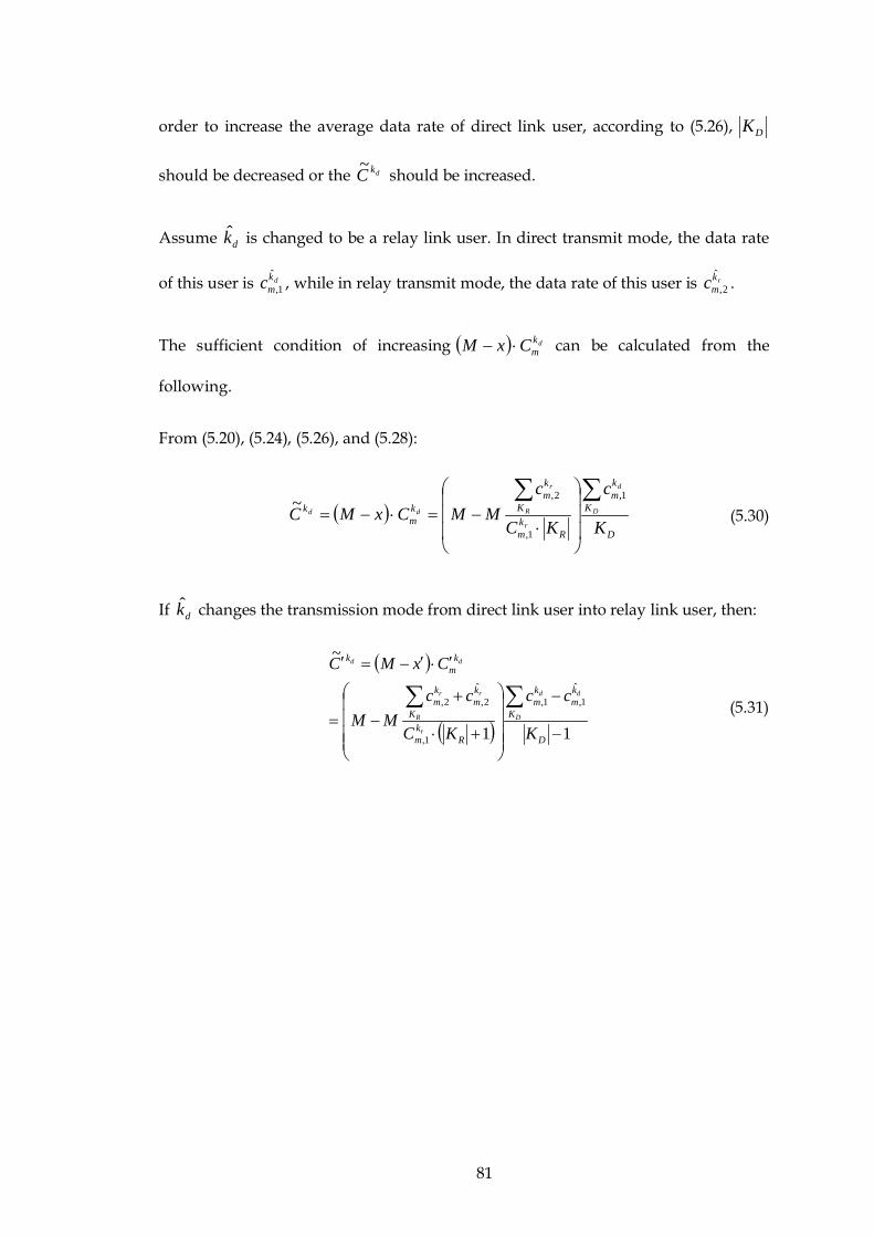
81
order to increase the average data rate of direct link user, according to (5.26), DK
should be decreased or the dkC~ should be increased.
Assume dk̂ is changed to be a relay link user. In direct transmit mode, the data rate
of this user is dkmc ˆ
1, , while in relay transmit mode, the data rate of this user is rkmc ˆ
2, .
The sufficient condition of increasing ( ) dkmCxM ⋅− can be calculated from the
following.
From (5.20), (5.24), (5.26), and (5.28):
( )D
K
km
Rkm
K
km
km
k
K
c
KC
cMMCxMC D
d
r
R
r
dd
∑∑
⋅−=⋅−=
1,
1,
2,~ (5.30)
If dk̂ changes the transmission mode from direct link user into relay link user, then:
( )
( ) 11
~
ˆ1,1,
1,
ˆ2,2,
−
−
+⋅
+−=
′⋅′−=′
∑∑D
km
K
km
Rkm
km
K
km
km
k
K
cc
KC
ccMM
CxMCd
D
d
r
r
R
r
dd
(5.31)

82
From (5.30) (5.31):
( )( )
( ) ( )
( )
( )
( )
⋅−⋅
⋅−⋅−⋅+⋅
−⋅
−⋅−⋅+⋅
=
⋅⋅
−⋅
−−+⋅
−⋅+⋅⋅
−⋅
=′⋅′−
⋅−
∑∑
∑∑∑ ∑
∑∑
∑∑
d
D
dr
R
rrr
D
d
D
d
R R
rrrr
d
D
dr
R
rr
D
d
R
rr
d
d
kmD
K
kmD
kmR
K
kmR
kmRR
km
K
km
K
kmD
K K
km
kmR
kmRR
km
DRkm
K
km
km
K
kmR
km
DRK
km
K
kmR
km
km
km
cKcKcKcKCKKC
ccKccKCKKC
KKccccKC
KKcCKC
CxMCxM
ˆ1,1,
ˆ2,2,1,
21,
1,1,2,2,1,2
1,
ˆ1,1,
ˆ2,2,1,
1,2,1,
1
11
(5.32)
From (5.32) it can be seen that if:
r
R
r kmR
K
km cKc ˆ
2,2, ⋅≥∑ and d
D
d kmD
K
km cKc ˆ
1,1, ⋅≥∑ (5.33)
then (5.32) is smaller than 1 and ( ) dkmCxM ⋅− will increase. In fact, (5.33) is a
sufficient condition but not a necessary one, but it is simple to be satisfied and easy
to implement.
Choosing the direct link user dk̂ who has the smallest large scale SINR, and if (5.33)
is satisfied changing dk̂ into a relay link user, will increase the average data rate of
direct link users. If this condition is not satisfied, select the second smallest SINR
direct link user, check if that fulfils the above condition to be a relay link user, and so
on.
5.4.2 Algorithm Procedure
Define the time interval T , called the algorithm execution interval which is longer
than one TTI. The LBRS algorithm will operate in each T as follows:
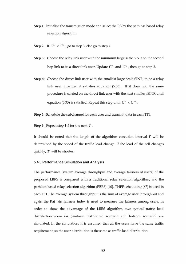
83
Step 1: Initialise the transmission mode and select the RS by the pathloss based relay
selection algorithm.
Step 2: If dr kk CC < , go to step 3, else go to step 4.
Step 3: Choose the relay link user with the minimum large scale SINR on the second
hop link to be a direct link user. Update rkC and dkC , then go to step 2.
Step 4: Choose the direct link user with the smallest large scale SINR, to be a relay
link user provided it satisfies equation (5.33). If it does not, the same
procedure is carried on the direct link user with the next smallest SINR until
equation (5.33) is satisfied. Repeat this step until dr kk CC < .
Step 5: Schedule the subchannel for each user and transmit data in each TTI.
Step 6: Repeat step 1-5 for the next T .
It should be noted that the length of the algorithm execution interval T will be
determined by the speed of the traffic load change. If the load of the cell changes
quickly, T will be shorter.
5.4.3 Performance Simulation and Analysis
The performance (system average throughput and average fairness of users) of the
proposed LBRS is compared with a traditional relay selection algorithm, and the
pathloss based relay selection algorithm (PBRS) [40]. THPF scheduling [67] is used in
each TTI. The average system throughput is the sum of average user throughput and
again the Raj Jain fairness index is used to measure the fairness among users. In
order to show the advantage of the LBRS algorithm, two typical traffic load
distribution scenarios (uniform distributed scenario and hotspot scenario) are
simulated. In the simulation, it is assumed that all the users have the same traffic
requirement, so the user distribution is the same as traffic load distribution.

84
With uniform distribution of users in the target area, using polar coordinates to
express the location of user ( )θρ , , it can be deduced that ),0(~ 22 RUρ , and
)2,0(~ πθ U [31]. A random drop of user location example is shown in Figure 5.6.
-0.5 -0.4 -0.3 -0.2 -0.1 0 0.1 0.2 0.3 0.4 0.5-0.5
-0.4
-0.3
-0.2
-0.1
0
0.1
0.2
0.3
0.4
0.5BSRSMS
Figure 5.6 Traffic load of uniform distribution
Figure 5.7 and Figure 5.8 show the performance comparison of these two algorithms
with different user numbers under uniform distribution. As the number of users
increases, the system average throughput increases and the fairness index decreases
in the long-term view. The PBRS gives a slightly better average throughput
compared with LBRS, but LBRS shows better fairness – this is especially true for a
larger number of users where there is little difference in throughput but the
improvement in fairness is maintained. For example, when there are 20 users in the
cell, the average throughput of LBRS is about 4.6% worse than that of PBRS but the
fairness index of LBRS is 8% more than that of LBRS; when the number of users
increased to 50, the average throughput of LBRS is about 4.8% worse than that of
PBRS but the fairness index of LBRS is 12% more than that of LBRS.
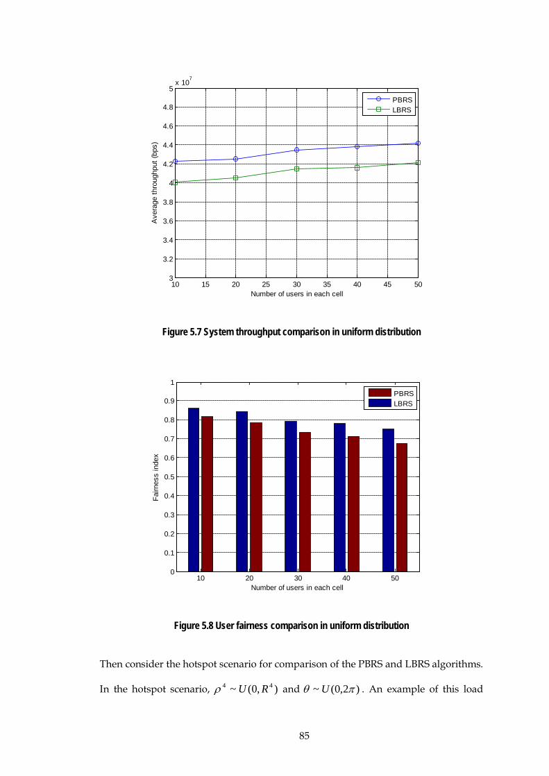
85
10 15 20 25 30 35 40 45 503
3.2
3.4
3.6
3.8
4
4.2
4.4
4.6
4.8
5x 10
7
Number of users in each cell
Ave
rage
thro
ughp
ut (b
ps)
PBRSLBRS
Figure 5.7 System throughput comparison in uniform distribution
10 20 30 40 500
0.1
0.2
0.3
0.4
0.5
0.6
0.7
0.8
0.9
1
Number of users in each cell
Fairn
ess
inde
x
PBRSLBRS
Figure 5.8 User fairness comparison in uniform distribution
Then consider the hotspot scenario for comparison of the PBRS and LBRS algorithms.
In the hotspot scenario, ),0(~ 44 RUρ and )2,0(~ πθ U . An example of this load

86
distribution is shown in Figure 5.9, where most of the users are distributed at the
edge of the cell.
-0.5 -0.4 -0.3 -0.2 -0.1 0 0.1 0.2 0.3 0.4 0.5-0.5
-0.4
-0.3
-0.2
-0.1
0
0.1
0.2
0.3
0.4
0.5BSRSMS
Figure 5.9 Traffic load of hotspot scenario
10 15 20 25 30 35 40 45 503
3.2
3.4
3.6
3.8
4
4.2
4.4
4.6
4.8
5x 10
7
Number of users in each cell
Ave
rage
thro
ughp
ut (b
ps)
PBRSLBRS
Figure 5.10 System throughput comparison in hotspot scenario

87
10 20 30 40 500
0.1
0.2
0.3
0.4
0.5
0.6
0.7
0.8
0.9
1
Number of users in each cell
Fairn
ess
inde
x
PBRSLBRS
Figure 5.11 Fairness index comparison in hotspot scenario
Figure 5.10 and Figure 5.11 show the performance comparison of the LBRS and PBRS
in the hotspot scenario. It can be seen that when the number of users increases, the
user fairness gain of LBRS will be enhanced, which is the same as the conclusions
drawn from Figure 5.7 and Figure 5.8. From the simulation results, it also can be seen
that the LBRS algorithm achieves better fairness gain in the hotspot scenario than
that with uniform distribution. When there are 50 users in the cell, the average
throughput with LBRS is about 8% less that of PBRS but the fairness index of LBRS is
20% better than that of PBRS.
These simulation results show that the LBRS algorithm can achieve better fairness
than the traditional relay selection algorithm in both typical traffic load distribution
scenarios.
5.5 Summary
This chapter studied the fairness radio resource allocation issue. A two-hop
proportional fairness algorithm which improves system throughput while

88
guaranteeing user data rate is proposed. In addition, a load based relay selection
algorithm which considered the fairness issue between direct link user and relay link
user is proposed.
This work was done without considering the power efficiency problem, and equal
power allocation is used in relay selection and subchannel allocation. Work on a
suitable power allocation scheme is given in the next chapter.

89
Chapter 6 Energy Efficient Power Allocation
The work in this chapter is new and entirely that of the author.
6.1 Introduction
In relay based cellular networks, under equal power allocation for BS and RS, the
subchannel capacity of the first hop link of an RS is not coupled with that of the
second hop link. In order to keep the data rate of the two hop links balanced, a two-
hop power allocation (THPA) algorithm is proposed to adjust the transmission
power of the BS and the RS dynamically according to the difference in data rates
between these two hop links. The aim of this algorithm is power efficiency at the
transmission node.
In a multi-cell OFDMA scenario, because the interference is inter-cell interference, the
performance of users at the cell edge is affected most. Therefore, a multi-cell power
allocation considering inter-cell interference has also been studied by the author and,
based on a multi-cell non-cooperative game model, a distributed multi-cell power
allocation algorithm has been implemented. Different utility functions are defined
for different optimisation objectives (system throughput and user fairness
respectively) and the existence and uniqueness of the Nash equilibrium as a solution
of the non-cooperative power allocation game is proved mathematically. The
performance of this algorithm has been investigated by simulation.
6.2 Power Allocation between Two-Hops
6.2.1 Existing problem
In a relay system, the data rate of each RS depends on the minimum of the first hop
link data rate (achieved data rate in the first time subslot) and the second hop link
data rate (achieved data rate in the second time subslot). The data rate of the two hop
links is usually different with equal power allocation. This is illustrated in Figure 6.1
where the transmission data rate for the two hop links at different TTI is compared.

90
0 10 20 30 40 50 60 70 80 90 1001
1.5
2
2.5
3
3.5
4
4.5
5
5.5x 10
4
Simulation Time (TTI)
Tran
smis
sion
bit
First hop of RSSecond hop of RS
Figure 6.1 Two-hop throughput of RS with equal power allocation
For two-hop link data rate balance, the transmission power of BS and RS can be
adjusted adaptively to make the data rate of the first hop link and the second hop
link matched to each other. If the data rate of the first hop link is smaller than that of
the second hop link, increasing the transmission power of the BS can increase the
data rate of the first hop link to the same value as the data rate of the second hop link,
and system throughput will be increased; on the other hand, decreasing the
transmission power of the RS can decrease the data rate of the second hop link to the
same value as the data rate of the first hop link, and transmission power will be
saved. If the data rate of the first hop link is larger than that of the second hop link,
the situation is similar, but the other way round.
In the two-hop power allocation (THPA) algorithm, the optimization target is power
efficiency in which the transmission power of the BS and RS is optimised to
minimize the total transmission power.

91
6.2.2 Two-Hop Power Allocation
For RS r , rM1 is the set of allocated subchannels on the first time subslot and rM 2 is
the set of allocated subchannels on the second time subslot, and rkM is the set of
subchannels allocated to the user rk .
The available data rate of the RS r is determined by the minimum transmission data
rate of the first hop link and the second hop link, which can be expressed as:
{ }rrr ccc 21 ,min= (6.1)
For the RS r , the data rate difference between the second hop link and the first hop
link is:
rrr ccc 12 −=∆ (6.2)
If 0<∆ rc , the data rate of the second hop link is smaller than the data rate of the
first hop link. While maintaining the system throughput, the transmission power of
the BS can be reduced so that the data rate of the second hop link matches that of the
first hop for each RS.
Let rmp 1,ˆ be the transmission power from the BS to the RS r on the subchannel
m ( )rMm 1∈ after THPA. Define rmp 1, as the transmission power from the BS to the
RS r on the subchannel m ( )rMm 1∈ with equal power allocation. The adjusted
power value can be calculated according to rc∆ .
From (5.2) (5.7), the rc∆ is:
Γ+−
Γ+=∆ ∑∑
∈∈2
1,1,22
1,1,2 1log
ˆ1log
11σσ
rm
rm
Mmm
rm
rm
Mmm
r pgB
pgBc
rr
(6.3)

92
Let rmc 1,∆ be the decreased data rate on the subchannel m ( )rMm 1∈ of the first hop
link of the RS r :
Γ+−
Γ+=∆ 2
1,1,22
1,1,21, 1log
ˆ1log
σσ
rm
rm
rm
rm
mrm
pgpgBc (6.4)
The total data rate change is the sum of the individual change on each subchannel, so:
∑∈
∆=∆rMm
rm
r cc1
1, (6.5)
For simplicity, let the reduced data rate on each allocated subchannel in the first time
subslot be equal; then
r
rrm M
cc1
1,∆
=∆ (6.6)
From (6.3)-(6.6), the transmission power from the BS to the RS r on the subchannel
m ( )rMm 1∈ after power allocation can be calculated as:
rm
rm
rm
Bc
rm gg
pp m
rm
1,
2
1,
2
1,1,
1,
2ˆ σσ Γ−
Γ+=
∆
(6.7)
If 0>∆ rc , the data rate of the second hop link is bigger than the data rate of the first
hop link. So the data rate of the second hop link can be reduced by rc∆ to match the
data rate of the first hop link of RS r by reducing the transmission power of RS, and
the system throughput is not changed.
In order to maintain the user fairness, the reduced rc∆ is proportionally distributed
among the MSs served by the RS r . Let the reduced data rate of the user rk is rkc∆ ,
so:

93
∑∈
∆=∆
rRr
r
rr
Kk
k
krk
cccc
2
2 (6.8)
Similar to the derivation of (6.7), the transmission power from the RS r to the user
rk on the subchannel m ( )rkMm∈ after power allocation rk
mp 2,ˆ becomes:
rr
rrkm
rk
rkm
km
km
MBc
km gg
pp2,
2
2,
2
2,2, 2ˆ σσ Γ−
Γ+=
∆
(6.9)
The adaptive two-hop power allocation algorithm will operate as follows:
Step 1: The subchannels of both the first and the second time subslots are assigned
by the THPF algorithm.
Step 2: Each RS r calculates the data rate of the first hop link rc1 and that of the
second hop link rc2 in terms of equal power allocation of BS and each RS.
Step 3: If 0<∆ rc , the transmission power of BS on the subchannel m ( )rMm 1∈
occupied by the RS r will be derived from (6.7), while the
transmission power of the RS r on the subchannel m ( )rMm 2∈ will
remain equivalent to the equal power allocation case.
Else, the transmission power of BS on the subchannels m ( )rMm 1∈
occupied by the RS r will be unchanged, and the transmission power
of RS r on the subchannel m ( )rkMm∈ will be calculated by (6.9)
instead.
Step 4: Downlink data packet will be sent with the transmission power of BS and RS
according to step 3.

94
6.2.3 Performance Simulation and Analysis
It has been pointed out that the throughput of each RS in the first hop link and that
in second hop link do not match each other in every TTI with equal power allocation
on every subchannel; this is shown in Figure 6.1 showing the simulation results on
the throughput comparison of two hop links without THPA.
In this section, the system performance under THPA is tested. Figure 6.2 is the
throughput comparison of two hop links with THPA. It can be seen that the
throughput of the first hop link and that of second hop link now match each other in
every TTI. The average data rate in the first hop link is 71018.3 × bit/s, and of the
average data rate in the second hop link is 71018.3 × bit/s as well. Since the
throughput is determined by the minimum of the capacity of the first hop link and
the second hop link of each RS, the system performance with the THPA is the same as
that with equal power allocation.
0 10 20 30 40 50 60 70 80 90 1001
1.5
2
2.5
3
3.5
4
4.5
5
5.5x 10
4
Simulation Time (TTI)
Tran
smis
sion
bit
First hop of RSSecond hop of RS
Figure 6.2 Two-hop throughput of RS with THPA

95
Figure 6.3 and Figure 6.4 shows that the transmission power of the BS and RSs with
the THPA algorithm is significantly reduced compared with that of equal power
allocation (EQPA).
In Figure 6.3, when the RSs are located at the edge of the cell, the amount of power
reduction for the BS is less than that when the RSs are 0.4 D to 0.5 D away from BS.
This is because the proposed THPA algorithm considered the power saving related
to relay link users, (when the RSs are located at the cell edge, the number of relay
link users is less than the number of relay link users when relay is located in the cell
centre) and the channel state of the second hop link is better than that of first hop
link. However, the total transmission power of RSs is greatly reduced when RSs are
at the edge of the cell because the channel state of the second hop link is better than
that of the first hop link, and RSs will reduce the power to balance the data rate
between the two hop links.
On the other hand, when RSs are located near the BS, the channel state of the second
hop link is poor so the transmission power of RSs almost remains the same as the
power with equal power allocation while the transmission power of the BS is
reduced.
Although power reduction of a component (BS or RS) varies with distance of the RS
from the BS, Figure 6.4 shows that the total power saving is approximately constant.
The total transmission power of BS plus six RSs with the THPA algorithm is reduced
roughly 30% compared to that of equal power allocation.

96
0.2 0.3 0.4 0.5 0.6 0.7 0.80
2
4
6
8
10
12
14
16
18
20
22
RS normalized distance
Ave
rage
tran
smis
sion
pow
er (W
)
BS power of EQPABS power of THPARS power of EQPARS power of THPA
Figure 6.3 BS/RS transmission power vs. RS normalized distance
0.2 0.3 0.4 0.5 0.6 0.7 0.80
5
10
15
20
25
30
35
Ave
rage
tran
smis
sion
pow
er (W
)
RS normalized distance
BS+RS power of EQPABS+RS power of THPA
Figure 6.4 Total transmission power vs. RS normalized distance
From Figure 6.3 to Figure 6.4 it can be seen that, THPA can effectively reduce
transmission power.

97
6.3 Power Allocation among Multi-Cells
THPA is only one aspect of the problem: although it balances the data rate on the
two hop links to minimize the transmission power, it does not consider inter-cell
interference or how to minimize the transmission power among multiple cells. Some
work on power allocation in OFDMA relay systems has been given in [64][65],
however, these algorithms only consider a single cell scenario and omit the co-
channel interference (CCI) in multiple cells. In this section, power allocation in a
multi-cell OFDMA relay system is considered and a distributed power allocation
algorithm based on non-cooperative game theory is determined.
6.3.1 Background of Game Theory
Game theory is a branch of applied mathematics which attempts to mathematically
capture behaviour in strategic situations in which an individual's success in making
choices depends on the choices of others [68].
Game theory was originally proposed by John von Neumann and Oskar
Morgenstern in 1944 in the book ‘Theory of games and economic behaviour’ [69]. In
the following decades, game theory has been developed into a wider area and is
widely recognized as an important tool in many fields.
In the communications area, game theory has been applied to analyze and solve
different problems in a broad number of areas such as cryptographic protocols
[70][71], peer to peer (P2P) systems [72], as well as wireless communications and
mobile networking [73][74][75][76]. Later in this section there is an explanation as to
how this work is different from previous use of game theory in OFDMA networks.
A game has players who each have a strategy that they use to try to achieve the
optimum utility.
Player k has a strategy set kS that consists of a number of individual strategies ks
so { }kk sS = and the player can decide which strategy from its set it can use. The

98
vector ( )nss ,,1 =s , is the strategy profile, i.e. the profile of the strategies of all the
users { }nk ,,2,1 = .
The utility level { }sku is decided by the strategy profile of all the players, i.e. it not
only depends on the strategy chosen by the player k ,but also on the strategies
chosen by all the other players.
There are two different types of games: cooperative and non-cooperative. This thesis
uses non-cooperative game theory as users are competing against each other [77] to
get the capacity they require, whereas in cooperative game theory users form
coalitions and contracts between them.
The game aims to find an equilibrium that gives the maximum utility; the equilibrium
is a set of strategies where users are unlikely to change their behaviour. Many
equilibrium concepts have been developed, but the most generally used is the Nash
equilibrium [77]. This uses the concept for equilibrium that, as a player knows the
equilibrium strategies of the others, it will know that it cannot improve its utility by
changing its own strategy if the other players keep theirs unchanged. This means
that each player chooses the optimal response according to the other players’
strategies and if any player changes its strategy independently, its utility will be
reduced.
A strategy profile ( )∗∗= nss ,...1*s is said to be a Nash Equilibrium if:
( )∗−− ′≥ kkkkkk ssussu ,),( ** ∗≠′∀ kk ss (6.10)
In setting up a non-cooperative game, the research is on how to maximize the
players’ utilities with given strategy sets and how to reach equilibrium.
A basic model for non-cooperative power control game in CDMA networks was first
proposed by D. Goodman [78][79], in which the quality of service (QoS) of a user is

99
the utility, and non-cooperative game theory is used to devise a power control
scheme to maximize the utilities. The interference in CDMA is mainly intra-cell
interference, while the interference in OFDMA systems is generally inter-cell
interference. Non-cooperative power allocation game is used for work on OFDMA
systems in [80] to maximize users’ utilities in a distributed way in multi-cell systems.
[81] considers the non-cooperative power allocation game in multi-cell OFDMA relay
networks, however, it considers power allocation only in the second time subslot and
only in slow fading channel scenarios.
There has not been related work that addresses the problems considered here.
6.3.2 Multi-Cell System Model
In OFDMA cellular systems, the subchannels are orthogonal to each other, so there
will be no intra-cell interference. The frequency reuse factor of OFDMA systems is
generally “1” to maximise the overall spectrum efficiency. However, this means that
co-channel interference (CCI) in co-frequency subchannels will be the dominant
inter-cell interference between adjacent cells and cause the performance of users at
the cell edge to deteriorate. Figure 6.5 shows an example of the downlink inter-cell
interference between two cells in the second hop link in relay OFDMA networks.
Figure 6.5 Downlink inter-cell interference in the second hop link
The layout of multiple cells as used in this research is shown in Figure 6.6.

100
3 1
2
0
4
5
6
8
9
12
11
13
14
15
16
17
18
7
10
Figure 6.6 Layout of multi-cell system
Notation used here is as follows:
total number of cells is N ;
total bandwidth is B ;
the number of subchannels is M , so the subchannel bandwidth is
MBBm = ;
( )Nn ,2,1∈ is the index of a cell;
s is the index of a transmitter in each cell (note that the use of s as an
index should not be confused with si as a strategy);
in the first time subslot the transmitter is BS ( 0=s ), and in the second
time subslot the transmitter is RS ( rs = , r is the index of RSs);
the time subslot is )2,1(∈i ;
the index of subchannel is ( )Mm ,2,1∈ ;
k is the index of a receiver in each cell:
• when the RS is a receiver, rk =
• the direct link user is dk
• the relay link user served by RS r is denoted as rk .

101
( )ksimnp ,
,, is transmission power on the subchannel m in the cell n between
the transmitter s and the receiver k at the thi time subslot;
( )ksimng ,
,, is the useful signal link gain on the subchannel m in the cell n
between the transmitter s and the receiver k at the thi time subslot;
( )ksimng ,
,,′′ is the interference link gain on the subchannel m between the
transmitter s′ in the cell ( )nnn ≠′′ and the receiver k in the cell n at the
thi time subslot.
The interference plus noise received by the transmitter s (BS or RS) and the receiver
k (RS or MS) in the thn cell on the subchannel m at the thi time subslot ( )ksimnI ,
,, is:
( ) ( ) ( )
{ }
2
,
,,,
,,,
,,, σ+= ∑
≠′′
′′′
′′
nnn
ksimn
ksimn
ksimn pgI (6.11)
in which, 2σ is the power of AWGN.
The signal to interference plus noise ratio (SINR) on the thm subchannel between the
transmitter s and the receiver k at the thi time subslot in the thn cell is:
( ) ( ) ( ) ( ), , , ,, , , , , , , ,s k s k s k s k
n m i n m i n m i n m ig p Iγ = (6.12)
The capacity of the thm subchannel between s and k of the cell n in the time subslot
i is:
( ) ( )( ), ,, , 2 , ,log 1s k s k
n m i m n m ic B γ= + (6.13)
The subchannels can be allocated with any scheduling algorithm. A fixed subchannel
allocation is used here to cancel the effect of scheduling on system performance. In

102
the cell n , for a direct link user dk , the achieved data rate is dknc and the achieved
data rates of the relay link user rk in the first hop link and second hop link are rknc 1,
and rknc 2, respectively. The available data rate of a relay link user rk
nc is determined by
the minimum capacity of the first hop link and the second hop link in DF relay [6],
which can be expressed as:
{ }rrr kn
kn
kn ccc 2,1, ,min= (6.14)
6.3.3 Non-Cooperative Power Allocation Game
In OFDMA systems, there is no intra-cell interference, but there is inter-cell
interference. So the power allocation problem of multi-cell OFDMA relay systems
can be viewed as a non-cooperative game, in which the BSs (RSs) in multiple cells
will compete with each other on co-frequency subchannels for channel capacity by
increasing the transmission power selfishly.
6.3.3.1
In OFDMA systems, the subchannels are independent, so the utility maximization of
one cell is equivalent to maximizing the utility on each subchannel in that cell. Thus,
the multi-cell non-cooperative power allocation game (NPAG) can be formulated on
each co-frequency subchannel. Furthermore, the BSs transmit data in the first time
subslot and the RSs transmit data in the second time subslot, so the NPAG can be
formulated as
Model of NPAG
{ } { }{ }[ ]BSmn
BSmn
BS upnG ,, ,,= in the first time subslot, and
{ } { }{ }[ ]RSmn
RSmn
RS upnG ,, ,,= in the second time subslot. In BSG , { }n is the set of co-
channel interference cells, i.e. a set of players competing with each other;
],[ max,
min,, mnmn
BSmn ppP = is the strategy set of transmission power of the BS on the thm
subchannel in the thn cell; ( )BSmN
BSm
BSm
BSm ppp ,,2,1 ,,, =P is the BS transmission power
vector of all the cells on the thm subchannel; BSmn,−P is the BS transmission power

103
vector on the thm subchannel of all the cells excluding the power BSmnp , in the thn cell.
So, the BS transmission power vector on the thm subchannel of all the cells can be
expressed as ( )BSmn
BSmn
BSm p ,, , −= PP . BS
mnu , is the utility of the BS on the thm subchannel in
the thn cell, and each cell will maximize its utility rationally. Similarly, n , RSmnp , and
RSmnu , are defined in RSG .
Since each transmitter prefers to increase its transmission power to increase its
capacity, this will also increase the interference and degrade the capacity of adjacent
cells in which users are using a co-frequency subchannel. Then the cells whose
capacities are affected also prefer to increase their transmission power to increase
their capacities. So a pricing factor is used in order to force transmitters in each cell
consider not only their own capacity but also control the interference to others [79].
The utility of the BS on the subchannel m in the thn cell can then be defined as:
( ) ( )( ) ( )kmn
BSkmnm
BSm
BSmn pBu ,0
1,,,0
1,,2, 1log αγ −+=P (6.15)
In the following, BSmnp , is used to represent ( )k
mnp ,01,, for simplicity and BSα is the
pricing factor of a BS (this is a positive scalar and can be considered to have units of
bps/W). With the introduction of BSα , a transmitter will not just increase the power
selfishly to increase its channel capacity, but also will consider the interference to
others. The larger BSα is, the higher the price for increasing power is, so each cell
will use attempt to use less transmission power, which causes less interference to
other cells.
In order to use the channel efficiently, the match issue between the second hop link
and the first hop link of the RS r should be considered. A match factor is introduced,

104
which is defined as the ratio of the first hop link capacity of the RS r and second hop
link capacity of the RS r in the cell n :
∑
∑
∈
∈=
rRr
r
rRr
r
Kk
kn
Kk
kn
rn c
c
2,
1,
β (6.16)
As the BS transmits data for both direct link users and RSs in the first time subslot,
the pricing factor for direct link users and RSs is different in the first time subslot,
which is:
⋅′
′=
nrrn
BS
BSBS
cell in the RSfor userlink direct for
βα
αα (6.17)
BSα′ is the basic pricing factor for both direct link user and RS. From (6.17) it can be
seen that the direct link users and the RSs use a different pricing factor to compete
for transmission power. When 1>rnβ , i.e., the channel capacity of the first hop link is
bigger than that of the second hop link, the BSα increases compared with the basic
pricing factor BSα′ . Therefore, the BS decreases its transmission power to the RS r to
match the capacity of the first hop link and that of the second hop link. The larger the
difference between the data rate of two hop links is, the bigger rnβ is; as a result, BSα
becomes bigger, and the transmission power is more strictly controlled. When 1<rnβ ,
the BS tends to increase its transmission power to increase the first hop link capacity
of RS to match that of the second hop link.
Similarly to (6.15), the utility of RS in the thn cell on the thm subchannel in the second
time subslot can be defined as:
( ) ( )( ) ( )krmn
RSkrmnm
RSm
RSmn pBu ,
2,,,
2,,2, 1log αγ −+=P (6.18)

105
in which, RSα is the basic pricing factor of the RS, which has the same function as
BSα and in the following parts, RSmnp , is used to represent ( )kr
mnp ,2,, for simplicity.
6.3.3.2
The widely used solution of non-cooperative game problem is the Nash equilibrium
Solution of NPAG
[79], the definition of which for this problem is:
BSmn
BSmn Pp ,, ∈′∀ , ( ) ( )BS
mnBSmn
BSmn
BSmn
BSmn
BSmn pupu ,,,,,, ,, −− ′≥ PP
The power vector BSmP is the Nash equilibrium of NPAG. In the Nash equilibrium,
given the power of other cells, a cell cannot improve its utility by changing its
individual power. So the Nash equilibrium is a point of balance that each player who
succeeds in a competition does not want to deviate from. The existence and
uniqueness of the Nash equilibrium point in NPAG are illustrated in this section.
The Nash equilibrium for NPAG exists in the first time subslot when the following
two conditions are satisfied [79]:
i) { }BSmnp , is a nonempty, convex and compact subset of a finite Euclidean space NR ;
ii) ( )BSm
BSmnu P, is continuous in BS
mP and quasi-concave in BSmP .
A subset of Euclidean space NR is called compact if it is closed and bounded [82].
Since the strategy BSmnp , of every BS is identified as ],[ max
,min,, mnmn
BSmn ppp ∈ and max
,min, mnmn pp ≠ ,
it is a nonempty, convex [82] and compact subset of NR . So the first condition is
satisfied.
For the second condition, ( )BSm
BSmnu P, is obviously a continuous function in BS
mP as
defined in (6.15). Thus it is only necessary to prove the quasi-concave property of
( )BSm
BSmnu P, .

106
Taking the first-order partial derivative of (6.15) with respect to BSmnp , for any { }nn∈
yields:
( ) ( )
( ) ( ) ( )BS
kmn
kmn
kmn
kmnm
BSmn
BSm
BSmn
pgIgB
pu
α−+
=∂
∂,0
1,,,0
1,,,0
1,,
,01,,
,
,
2lnP
(6.19)
The second-order partial derivative of (6.15) with respect to BSmnp , for any { }nn∈ is
( ) ( )( )
( ) ( ) ( )( ) 02ln 2,0
1,,,0
1,,,0
1,,
2,01,,
,2,
2
<+
−=
∂∂
kmn
kmn
kmn
kmnm
BSmn
BSm
BSmn
pgIgB
pu P
(6.20)
From (6.20), ( )BSm
BSmnu P, is strictly concave in BS
mP , thus it is strictly quasi-concave in
BSmP as well [83]. Since both conditions of the existence of Nash equilibrium are
satisfied, the Nash equilibrium exists in NPAG.
The Nash equilibrium solution of NPAG is ( )BSmn
BSmn
Ppu
BSmn
BSmn
,,,,
maxarg P∈
. For a continuous
function, the necessary condition for a first-order optimization is:
( ) 0,, =∂∂ BSmn
BSm
BSmn pu P (6.21)
From (6.19):
( )
( )kmn
kmn
BSmBS
mn gIB
p ,01,,
,01,,
, 2ln−
⋅=
α (6.22)
If BSmnp , from (6.22) is within ],[ max
,min, mnmn pp , BS
mnp , is the Nash equilibrium solution of
NPAG in the first time subslot; otherwise, min,mnp or max
,mnp are Nash equilibrium
solution of NPAG in the first time subslot.
Next, the uniqueness of Nash equilibrium of NPAG in the first time subslot must be
considered. If (6.22) converges to a unique solution, the Nash equilibrium of NPAG

107
is unique as (6.22) is the Nash equilibrium of NPAG. From (6.12), (6.22) can be
rewritten as:
( )kmn
BSmn
BSmBS
mnpBp ,0
1,,
,, 2ln γα
−⋅
= (6.23)
The iterative expression of BSmnp , can be expressed as:
( ) ( )( ) ( )1
12ln ,0
1,,
,, −
−−
⋅=
ttpBtp k
mn
BSmn
BSmBS
mn γα (6.24)
In order to verify whether (6.24) converges to a unique solution, it is necessary to
prove the convergence of the difference between two adjacent iterations. From (6.11)
and (6.23) the difference between the tht )1( + and the tht iteration is:
( ) ( )( ) ( ) ( ) ( ) ( )( )
{ }( )k
mn
nnn
kmn
kmn
kmn
BSmn
BSmn g
tptpgtptp ,0
1,,
,
,01,,
,01,,
,01,,
,,
11
∑≠′′
′′′ −−=−+ (6.25)
If there exists infinitely smallε such that ( ) ( ) ε≤−− 1,, tptp BSmn
BSmn ,then:
( ) ( ) ( )
{ }
( )kmn
nnn
ksmn
BSmn
BSmn ggtptp ,0
1,,,
,1,,,, 1 ∑
≠′′
′′<−+ ε (6.26)
If ( ) ( )
{ }1
,
,1,,
,01,, >∑
≠′′
′′
nnn
ksmn
kmn gg , then (6.24) is convergent. This condition can be transferred
into the request of each user’s SINR and can be realized through the admission
control (if the SINR of a user is higher than 1, i.e., 0 dB which can be achieved easily
[84], this user will be allowed to access the system, through the access control). It
means that when ( ) ( )
{ }1
,
,1,,
,01,, >∑
≠′′
′′
nnn
ksmn
kmn gg the uniqueness of the Nash equilibrium of
NPAG in the first time subslot can be satisfied.
Similarly, the existence and uniqueness of the NPAG Nash equilibrium
{ } { }{ }[ ]RSmn
RSmn
RS upnG ,, ,,= in the second time subslot can be satisfied as well, and the
iterative expression of RSmnp , can be expressed as:

108
( ) ( )( ) ( )1
12ln ,
2,,
,, −
−−
⋅=
ttpBtp kr
mn
RSmn
RSmRS
mn γα (6.27)
6.3.3.3
The process of the NPAG algorithm is given as follows:
Process of NPAG
Step 1: On each subchannel m , initialize transmission power 0)0( =BSmΡ , 0)0( =RS
mΡ ,
and set iterative convergence parameter ε to be very small so that ε tends to
0 ( 0+→ε ).
Step 2: Let 0=t . Execute NPAG in the second time subslot.
Step 3: Let 1+= tt , calculate )(tRSmΡ according to (6.27).
Step 4: If ε<−− )1()( tt RSm
RSm ΡΡ , the NPAG of RS is over, )(tRS
mRSm ΡΡ = is the power
allocation result of RSs on the subchannel m , and go to step 5; otherwise, go
to step 3.
Step 5: Calculate the second hop link data rate of relay link users according to RSmΡ in
step 4, and update the match factor rnβ of the RS r in the cell n .
Step 6: Execute NPAG in the first time subslot. Let 0=t .
Step 7: Let 1+= tt , calculate )(tBSmΡ according to (6.24).
Step 8: If, ε<−− )1()( tt BSm
BSm ΡΡ , the NPAG of BS is over, )(tBS
mBSm ΡΡ = is the power
allocation results of BS on the subchannel m , and go to step 9; otherwise, go
to step 7.
Step 9: Calculate the first hop link data rate of relay link users and that of the direct
link users according to BSmΡ in step 8.

109
It can be seen that steps 1-9 are performed in a distributed manner by each cell and
different cells only need to exchange co-channel SINR information. The complexity
of this algorithm depends on the number of cells but not on the number of users
within the cell.
6.3.3.4
A multi-cell downlink OFDMA relay system is simulated. Wrap-around technology
is used for multi-cell interference, and the channel model [10] includes shadow
fading, large scale pathloss, and multi-path fading, as discussed in section 3.2. In
each single cell, one BS positioned in the centre of cell and 6 RSs are uniformly
distributed in the cell, located at 0.5 cell radius away from the BS; multiple users are
uniformly distributed across the cell. Detailed simulation parameters are as shown in
Table 3.1.
Performance Simulation and Analysis
First, in order to examine the second hop link average data rate of relay link users
with different RS basic pricing factors, the limitation of the first hop link data rate of
the relay link user is omitted, and assume that the end to end data rate of relay link
user is only decided by the data rate of second hop link here. Figure 6.7 shows that
the second hop link data rate increases first and then decreases with increasing RS
basic pricing factor. Figure 6.8 shows the simulation results of RS transmission
power with varying RS basic pricing factor compared with that with equal power
allocation (EQPA), in which RS transmission power decreases significantly as the RS
basic pricing factor increases.

110
0 0.5 1.5 2.5 3.5 4.5 5.5 6.5
x 105
1
1.02
1.04
1.06
1.08
1.1
1.12
1.14
1.16
1.18
1.2x 10
7
RS pricing factor
2 ho
p av
erag
e th
roug
hput
(bps
)
1-hop EQPA 2-hop NPAG1-hop EQPA 2-hop EQPA
Figure 6.7 The second hop average throughput vs. RS basic pricing factor
0 0.5 1.5 2.5 3.5 4.5 5.5 6.5
x 105
0
2
4
6
8
10
12
RS pricing factor
Ave
rage
tran
smis
sion
pow
er o
f RS
(W)
1-hop EQPA 2-hop EQPA1-hop EQPA 2-hop NPAG
Figure 6.8 RS power vs. RS basic pricing factor
From Figure 6.7 and Figure 6.8, it can be seen that, when the basic pricing factor
equals zero, NPAG of RS will converge to the RS equal power allocation. The

111
maximum second hop link data rate of NPAG is achieved when the basic price factor
is about 510×2.5 , where the data rate is increased by 4.5% compared with that of
equal power allocation of RS and the average transmission power of RS is reduced
by 24% compared with that of equal power allocation. The RS basic price factor can
be considered as the price paid for each unit of power, i.e., the higher the RS basic
pricing factor, the more expensive it is for one RS to increase its throughput by
increasing transmission power. When the RS basic pricing factor exceeds a certain
threshold ( 510×2.5 in the simulation), the transmission power of RS tends to
converge to a smaller value, which causes the second hop link average data rate to
decrease.
The effect of the BS basic pricing factor on system performance is examined in Figure
6.9 - Figure 6.11, with optimal RS pricing factor ( 510×2.5 as explained above).
0 1 2 3 4 5 6 7
x 105
0.9
0.92
0.94
0.96
0.98
1
1.02
1.04
1.06
1.08
1.1x 10
7
BS pricing factor
Ave
rage
thro
ughp
ut in
eac
h ce
ll (b
ps)
1-hop NPAG 2-hop NPAG1-hop EQPA 2-hop NPAG
Figure 6.9 System throughput vs. BS basic pricing factor (fixed RS pricing factor)

112
0 1 2 3 4 5 6 7
x 105
0
0.1
0.2
0.3
0.4
0.5
BS pricing factor
Fairn
ess
inde
x
1-hop EQPA 2-hop NPAG1-hop NPAG 2-hop NPAG
Figure 6.10 User fairness vs. BS basic pricing factor (fixed RS pricing factor)
0 1 2 3 4 5 6 7
x 105
0
2
4
6
8
10
12
14
16
18
20
22
BS pricing factor
Ave
rage
tran
smis
sion
pow
er o
f BS
(W)
1-hop EQPA 2-hop NPAG1-hop NPAG 2-hop NPAG
Figure 6.11 BS power vs. BS basic pricing factor (fixed RS pricing factor)
It can be seen from Figure 6.9 that when the BS basic pricing factor is zero, the system
throughput is the same as that given by equal power allocation, and system

113
throughput increases first and then decreases with increasing BS pricing factor.
When the BS basic pricing factor equals 510×3 , the largest system throughput gain is
obtained and increases to 3% compared with that of BS equal power allocation. The
fairness index deceases with increasing BS pricing factor, as shown in Figure 6.10.
Figure 6.11 is the average BS transmission power under different BS basic pricing
factor (RS basic pricing factor equals 510×2.5 ), which shows that the BS average
transmission power decreases as pricing factor rises. In Figure 6.11, it can also be
seen that, when BS basic pricing factor is 510×3 and RS basic pricing factor is
510×2.5 , the average power of a BS will reduce by 25% compared with that of BS
using equal power allocation. With a BS basic pricing factor higher than 510×7 , the
BS transmission power is so small that the system throughput gain of NPAG will
decrease, and the average throughput of NPAG would be smaller even than that of
equal power allocation. It is not hard to understand that with a very high price,
nobody wants to spend much on power for data transmission.
In Figure 6.12 – Figure 6.14, the system performance of NPAG is compared with
equal power allocation on each subchannel (EQPA) with different user numbers. In
the simulation, the BS basic pricing factor is 5103× and RS basic pricing factor is
5105.2 × , the values at which maximum throughput will be obtained.
Figure 6.12 is the system throughput of each cell with different user numbers. At first,
the system throughput increases directly with the number of uses, but after a certain
number is reached the throughput saturates and then decreases. This is because the
larger the user number, the bigger the multi-user diversity gain, but, as the Round
Robin scheduling tries to keep user fairness, the system throughput will decrease as
the number gets too large. It can be seen that the throughput of NPAG is nearly 4%
larger than that of EQPA.

114
10 15 20 25 30 358
8.5
9
9.5
10
10.5
11x 10
6
Number of users in each cell
Ave
rage
thro
ughp
ut o
f eac
h ce
ll (b
ps)
EQPANPAG
Figure 6.12 System throughput vs. number of users in each cell
10 15 20 25 30 350
5
10
15
20
25
Number of users in each cell
Ave
rage
tran
smis
sion
pow
er in
eac
h ce
ll (W
)
EQPA-BSNPAG-BSEQPA-RSNPAG-RS
Figure 6.13 Transmission power vs. number of users in each cell

115
10 15 20 25 30 350
0.05
0.1
0.15
0.2
0.25
0.3
0.35
0.4
0.45
0.5
Number of users in each cell
Fairn
ess
inde
x
NPAGEQPA
Figure 6.14 Fairness index vs. number of users in each cell
Figure 6.13 shows the average transmission power of BS and RS under EQPA and
NPAG. Compared with EQPA, it is clear that the transmission powers of BS and RS
are reduced greatly by the use of NPAG, in which, the overall power (BS power plus
and RSs power) will be reduced by about 25%.
The user fairness index with different user numbers is shown in Figure 6.14. It can be
seen that the NPAG will decrease the user fairness compared with EQPA, which is
consistent with the result of Figure 6.10. The user fairness of NPAG is nearly 4% less
than that of EQPA, but this reduction is much less than the improvement in power
saving.
The simulation results show that system throughput is improved and transmission
power is reduced compared with that of EQPA. This is important as while power
saving is important the performance seen by the users needs to be maintained for the
system to be acceptable.

116
6.3.4 Non-Cooperative Power Allocation Game for Fairness
In the previous section, both the power allocation game in the first time subslot and
the second time subslot are defined in a fast-fading channel scenario. The multi-cell
non-cooperative power allocation game can increase the system throughput and
reduce power consumption but will also lead to a reduction in the data rate fairness
among users. The reason is that by the utility function defined in (6.15) and (6.18), the
users with good channel conditions will be allocated more transmission power.
However, the cell edge users will suffer larger co-channel interference than that of
cell centre users and have a worse channel condition than that of cell central users,
which means that the cell edge users will suffer lower data rates, so it is unfair for the
cell edge users. In this section, a novel utility function to improve the user fairness is
defined.
6.3.4.1
Based on the non-cooperative power allocation game model constructed in
Utility Definition for User Fairness
6.3.3.1,
the pricing factors defined for the BSs and for the RSs are modified to take into
account the average data rate of receivers for fairness.
The utility of the thn BS on the subchannel m can be defined as:
( ) ( )( ) ( ) ( )kmn
kn
BSkmnm
BSm
BSmn pRBu ,0
1,,,0,0
1,,2, 1log αγ −+=P (6.28)
in the following, BSmnp , is used to represent ( )mk
mnp ,01,, for simplicity and BSα is the BS
pricing factor, which is defined the same as in (6.17). ( )knR ,0 is the normalised average
data rate of the receiver k in the cell n , which is:
( )
∑=
= K
k
kn
knk
n
cK
cR
1
,0
1 (6.29)

117
If the receiver k is a direct link user, dkn
kn cc = . Since the RS will receive the data
from BS, retransmitting this data to a relay link user, the RS will act as a receiver in
the first time subslot. So the average data rate of all the users served by the RS r is
used to represent the average data rate of the RS r :
r
RRr
r
R
Kk
kn
rn K
cc
∑∈=
(6.30)
In (6.28), the ( )kn
BS R ,0α is called the modified pricing factor of BS. With the
introduction of the normalised average data rate ( )knR ,0 to the pricing factor BSα , a
transmitter will not just increase its power selfishly to increase the channel capacity,
but will consider the interference to other cells; i.e. it will take a view of the whole
system. The larger ( )kn
BS R ,0α is, the higher the price that will be incurred for
increasing power; therefore the BS in each cell prefers to use less power, causing less
interference to other cells. The modified pricing factor of a BS is adjusted by the
normalized average data rate of the receiver k which occupies the subchannel m . If
a receiver has a low average data rate, the modified pricing factor will be decreased:
as a result, the algorithm will allow the transmitter to use more power to this receiver
and hence obtain a higher throughput.
As a BS transmits data for both direct link users and RSs in the first time subslot, the
modified pricing factor ( )kn
BS R ,0α for direct link users and RSs is different in the first
time subslot, which is:
( )( )
( )
′
′=
nrRR
Rk
nrn
BS
kn
BSk
nBS
cellin RSfor
userlink direct for ,0
,0,0
βα
αα (6.31)
in which, BSα′ is the basic pricing factor of BS, rnβ is the match factor of the RS r in
the cell n defined in (6.16). ( ) ,0 kn
BS Rα′ is the modified pricing factor for a direct link
user, and ( )kn
rn
BS R ,0βα′ is the modified pricing factor for a RS. From (6.28) and (6.31),

118
it can be seen that direct link users and the RSs use different prices to compete for
transmission power. When 1>rnβ , the achieved data rate of RS r of the first hop
link is bigger than that of the second hop link, the value of ( )kn
rn
BS R ,0βα ′ will increase
compared with ( )kn
BS R ,0α ′ . Therefore, the BS can decrease its transmission power for
matching the capacity of the first hop link and that of the second hop link of RS r .
The larger the difference between the data rate of two hop links, the bigger is rnβ ; as
a result, ( )kn
rn
BS R ,0βα′ becomes larger, and the transmission power is more strictly
controlled. When 1<rnβ , the BS tends to increase its transmission power to increase
the first hop link capacity of a RS to match that of the second hop link.
Similarly to (6.28), the utility of a RS in the thn cell on the thm subchannel in the
second time subslot can be defined as:
( ) ( )( ) ( ) ( )krmn
krn
RSkrmnm
RSm
RSmn pRBu r ,
2,,,,
2,,2, 1log αγ −+=P (6.32)
in which, RSα is the basic pricing factor of RS, ( )rkrnR , is the normalised average data
rate of the receiver rk in the cell n , ( )rkrn
RS R ,α is the modified pricing factor of RS,
and in the following, RSmnp , is used to represent ( )kr
mnp ,2,, for simplicity. ( )rkr
nR , is defined
by:
( )
∑=
= K
k
kn
knkr
n
cK
cRr
r
1
,
1 (6.33)
6.3.4.2
The existence and uniqueness of the Nash equilibrium point in NPAG-F is the same
as that of NPAG. The Nash equilibrium solution of NPAG in the first time subslot is
Solution of NPAG-F
( )BSmn
BSmn
Ppu
BSmn
BSmn
,,,,
maxarg P∈
.

119
For a continuous function, the necessary condition for a first order optimization is:
( ) 0,, =∂∂ BSmn
BSm
BSmn pu P (6.34)
Taking the first-order partial derivative of (6.28) with respect to BSmnp , for any { }nn∈
yields:
( ) ( )
( ) ( ) ( )( )kn
BSk
mnk
mnk
mn
kmnm
BSmn
BSm
BSmn R
pgIgB
pu ,0
,01,,
,01,,
,01,,
,01,,
,
,
2lnα−
+=
∂
∂ P (6.35)
From (6.34) and (6.35):
( ) ( )kmn
BSmn
kn
BSmBS
mnp
RBp ,0
1,,
,,0, 2ln γα−
⋅⋅= (6.36)
Using the same method to get (6.24), then the iterative expression of BSmnp , can be
expressed as:
( ) ( )( )( )
( ) ( )11
12ln ,01,,
,,0, −
−−
−⋅⋅=
ttp
tRBtp k
mn
BSmn
kn
BSmBS
mn γα (6.37)
Similarly, the iterative expression of RSmnp , can be expressed as:
( ) ( )( )( )
( )( )11
12ln ,2,,
,,, −
−−
−⋅⋅=
ttp
tRBtp
mm krmn
RSmn
krn
RSmRS
mn γα (6.38)
The process of the NPAG-F is same as NPAG described in session 6.3.3.3.
6.3.4.3
Round Robin scheduling is used for subchannel allocation. The system average
throughput is the sum of average throughput achieved by each user in one cell. The
Raj Jain fairness index
Performance Simulation and Analysis
(5.18) is used as before to measure the fairness among users. In
the simulation, the BS basic pricing factor BSα′ and the RS basic pricing factor RSα
are the algorithm factors of NPAG-F. The system performance under different

120
pricing factors of BS and RS are compared with the equal power allocation with
maximum transmission power limitation.
Figure 6.15 shows the effect of the BS basic pricing factor and RS basic pricing factor
on the system throughput. Increasing the BS basic pricing factor or RS basic pricing
factor will decrease the average throughput.
Figure 6.16 is the simulation result on user fairness. The user fairness increases first
and decreases later with increasing BS basic pricing factor or RS basic pricing factor,
but the change is quite small. The optimal user fairness point varies with different BS
basic pricing factors if the RS pricing factor is fixed. When BSα′ = 510×7 and RSα =
510×5 the user fairness index is about 0.49, and that of equal power allocation is
about 0.41, an increase of more than 20%.
5 5.5 6 6.5 7 7.5 8 8.5 9 9.5 10
x 105
7
7.5
8
8.5
9
9.5
10x 10
6
BS pricing factor
Ave
rage
thro
ughp
ut o
f eac
h ce
ll (b
ps)
EQPAconstant of RS 300000constant of RS 500000constant of RS 800000
Figure 6.15 System throughput vs. BS basic pricing factor

121
5 5.5 6 6.5 7 7.5 8 8.5 9 9.5 10
x 105
0.4
0.41
0.42
0.43
0.44
0.45
0.46
0.47
0.48
0.49
0.5
BS pricing factor
Fairn
ess
inde
x
EQPAconstant of RS 300000constant of RS 500000constant of RS 800000
Figure 6.16 User fairness vs. BS basic pricing factor
Figure 6.17 and Figure 6.18 show the average transmission power of BS and RS
respectively, both of which reduce with increasing respective basic pricing factor.
5 5.5 6 6.5 7 7.5 8 8.5 9 9.5 10
x 105
10
12
14
16
18
20
22
BS pricing factor
BS
tran
smis
sion
pow
er (w
)
EQPAconstant of RS 300000constant of RS 500000constant of RS 800000
Figure 6.17 BS transmission power vs. BS basic pricing factor

122
5 5.5 6 6.5 7 7.5 8 8.5 9 9.5 10
x 105
0
2
4
6
8
10
12
BS pricing factor
RS
tran
smis
sion
pow
er (w
)
EQPAconstant of RS 300000constant of RS 500000constant of RS 800000
Figure 6.18 RS transmission power vs. BS basic pricing factor
Under equal power allocation, the transmission power of BS is 20 W and that of RS is
10 W, so the energy is reduced greatly when NPAG-F is used.
Table 6.1: RS basic pricing factor is 300,000
BS basic pricing factor BSα′
500,000 600,000 700,000 800,000 900,000 1000,000 Fairness +18.6% +19.1% +19.0% +18.7% +18.0% +17.2%
Throughput -5.7% -7.3% -9% -10.6% -12.3% -13.9%
Table 6.2: RS basic pricing factor is 500,000
BS constant pricing factor BSα′
500,000 600,000 700,000 800,000 900,000 1000,000 Fairness +18.9% +19.41% +19.43% +19.1% +18.5% +17.8%
Throughput -6.2% -8.4% -10.0% -11.7% -13.3% -15.0%
Table 6.3: RS basic pricing factor is 800,000
BS constant pricing factor BSα′

123
From the simulation results, it can be seen that there should be an optimal point
which will achieve a best tradeoff between user fairness and system throughput.
From Table 6.1-Table 6.3, the optimal point is when BSα′ = 510×6 and RSα = 510×3 ,
in which case the user fairness is increased 19.1% and throughput is decreased 7.3%.
6.4 Joint Power Allocation of THPA and NPAG
This section gives a joint distributed multi-cell power allocation (DMPA) algorithm
which is a combination of non-cooperative power allocation game (NPAG) and two-
hop power allocation (THPA) for energy efficiency and throughput improvement.
6.4.1 Algorithm Procedure
The process of the DMPA algorithm is given as following:
Step 1: On each subchannel m , initialize transmission power 0)0( =BSmΡ , 0)0( =RS
mΡ ,
and set iterative convergence parameter ε to be very small so that ε tends
to 0 ( 0+→ε ).
Step 2: Let 0=t . Execute NPAG in the second time subslot.
Step 3: Let 1+= tt , calculate )(tRSmΡ according to (6.27).
Step 4: If ε<−− )1()( tt RSm
RSm ΡΡ , the NPAG of RS is over, )(tRS
mRSm ΡΡ = is the power
allocation result of RSs on the subchannel m , and go to step 5; otherwise, go
to step 3.
500,000 600,000 700,000 800,000 900,000 1000,000 Fairness +18.2% +18.6% +18.6% +18.2% +17.5% +16.8%
Throughput -9% -11.2% -13.3% -15.5% -17.2% -18.8%

124
Step 5: Calculate the second hop link data rate of relay link users according to RSmΡ in
the step 4, and update the match factor rnβ of the RS r in the cell n .
Step 6: Execute NPAG in the first time subslot. Let 0=t .
Step 7: Let 1+= tt , calculate )(tBSmΡ according to (6.24).
Step 8: If, ε<−− )1()( tt BSm
BSm ΡΡ , the NPAG of BS is over, )(tBS
mBSm ΡΡ = is the power
allocation results of BS on the subchannel m , and go to step 9; otherwise, go
to step 7.
Step 9: Calculate the first hop link data rate of relay link users and that of the direct
link users according to BSmΡ in step 8.
Step 10: Calculates rc∆ from (6.2) for RS r in the cell n . If 0<∆ rc go to step 11, else
go to step 12 .
Step 11: The BS transmission power will be derived from (6.7), while the RS
transmission power remains as RSmΡ .
Step 12: The RS transmission power will be calculated by (6.9), and the transmission
power of BS is unchanged.
6.4.2 Performance Simulation and Analysis
The system throughput and transmission power of BS and RS of DMPA are
compared with two schemes: one is equal power allocation on each subchannel
(named EQPA), and the other is NPAG (as in section 6.3.3). Round Robin scheduling
is used for subchannel allocation. In the simulation, the BS basic pricing factor is
5103× and the RS basic pricing factor is 5105.2 × (these values give maximum
throughput as shown in section 6.3.3.4).

125
Figure 6.19 is the average throughput of each cell with different numbers of users.
The system throughput increases at first as the number of users increases and then
decreases. This is because multi-user diversity gain occurs as the number of users
gets bigger; however, as the Round Robin scheduling aims to keep user fairness,
making the number of users too large will decrease the system throughput. It can be
seen that the throughput of DMPA is nearly 4% larger than that of EQPA, and the
throughput of DMPA improves almost 1% over that of NPAG.
10 15 20 25 30 358
8.5
9
9.5
10
10.5
11x 10
6
Number of users in each cell
Ave
rage
thro
ughp
ut o
f eac
h ce
ll (b
ps)
EQPANPAGDMPA
Figure 6.19 System throughput vs. number of users in each cell
Figure 6.20 is the comparison of performance of average power of BS with different
numbers of users for the EQPA, NPAG and DMPA algorithms. Figure 6.21 is the
comparison of average power of RS among EQPA, NPAG and DMPA algorithms
respectively. Compared with EQPA, both the power of BS and RS of NPAG and
DMPA are greatly reduced. The DMPA consumes the smallest power both on BS and
on RS. From Figure 6.21, compared with EQPA, it can be seen that the RS power
saving of DMPA is 40% and the RS power saving of NPAG is 25%.

126
10 15 20 25 30 352
4
6
8
10
12
14
16
18
20
22
Number of users in each cell
Tran
smis
sion
pow
er o
f BS
(W)
EQPANPAGDMPA
Figure 6.20 BS transmission power vs. number of users in each cell
10 15 20 25 30 350
2
4
6
8
10
12
Number of users in each cell
Tran
smis
sion
pow
er o
f RS
(W)
EQPANPAGDMPA
Figure 6.21 RS transmission power vs. number of users in each cell
Overall, the DMPA in the multi-cell scenario not only saves energy, but also
improves system throughput. This is because, using THPA will decrease the

127
transmission power of the BS or RS to match the data rates of the two-hop links. This
will not decrease the system throughput of the cell but will reduce the interference to
other cells.
6.5 Summary
An adaptive power allocation algorithm called two-hop power allocation (THPA)
has been proposed. The transmission power of BS and RS decreases greatly but the
achieved system throughput remains the same as that with equal power allocation,
which is verified by the simulation results.
Subsequently, the power allocation for multiple cells with co-channel interference in
OFDMA relay networks is studied. A non-cooperative power allocation game is
defined for maximizing throughput and reducing co-frequency interference.
Next, the user fairness problem is considered for multi-cell OFDMA relay systems
with co-channel interference. A novel utility function is defined for user fairness.
Compared with equal power allocation, the user fairness is improved greatly with
only a small impact on system throughput; importantly with current concerns on
energy efficiency, the transmission power of the BS and the RSs is reduced greatly.
Besides, the joint power allocation algorithm which considers power allocation
between multi-cell and power allocation between two-hop is given, in which THPA
and NPAG is combined. From the simulation analysis, the joint power allocation
algorithm can reduced the transmission power efficiently and increase the system
throughput. This is considered further in the next chapter where a more systematic
study of combining the techniques researched in this thesis is presented.

128
Chapter 7 Joint Radio Resource Allocation Algorithm
In the earlier chapters, different individual techniques for increasing system
throughput, improving user fairness and energy efficiency are proposed: in Chapter
5, a novel relay selection algorithm (LBRS), and a subchannel allocation algorithm
(THPF) are given to improve user fairness; the emphasis in Chapter 6 is on energy
efficient power allocation with a two-hop power allocation algorithm (THPA) and a
multi-cell power allocation algorithm (NPAG or NPAG-F), plus an initial
investigation of combining NPAG and THPA. In this chapter, the proposed radio
resource allocation algorithms are combined with different algorithms and the
system performance (throughput, user fairness, and energy efficiency) is investigated.
The optimization target of NPAG is increasing the system throughput and that of
NPAG-F is improving the user fairness. By using different subchannel allocation, a
different power allocation result will be obtained after carrying out the NPAG (or
NPAG-F) algorithm. In this chapter, different combinations of relay selection,
subchannel allocation, power allocation between hops and power allocation between
cells are considered (as shown in Table 7.1).
Table 7.1 Joint Algorithms Used for Comparison
Joint algorithm name Relay selection Subchannel allocation
Power allocation between hops
Power allocation between cells
LRTN LBRS RR THPA NPAG LTTN LBRS THPF THPA NPAG PRNG PBRS RR EQPA NPAG PTNG PBRS THPF EQPA NPAG LRTN-F LBRS RR THPA NPAG-F LTTN-F LBRS THPF THPA NPAG-F PRNG-F PBRS RR EQPA NPAG-F PTNG-F PBRS THPF EQPA NPAG-F PREQ PBRS RR EQPA EQPA PTEQ PBRS THPF EQPA EQPA
129
The comparisons shown in this chapter are:
1) LRTN, PRNG and PREQ
2) LTTN, PTNG and PTEQ
3) LRTN and LTTN
4) LRTN-F, PRNG-F and PREQ
5) LTTN-F, PTNG-F and PTEQ
6) LRTN-F, LTTN-F
7) LTTN and LTTN-F
In (1), the scheduling algorithm is the RR algorithm, and different relay selection
algorithms are combined with the NPAG algorithm. PREQ, which is composed of
traditional algorithms (RR, PBRS and equal power allocation), is compared with the
proposed algorithms. In (2), the THPF algorithm is used instead of RR algorithm in
(1). In (3) different scheduling algorithms (RR and THPF) are combined with NPAG,
LBRS and THPA respectively. Similarly, in (4)-(6), the NPAG-F algorithm is used
instead of NPAG in (1)-(3) to allow the target of improved fairness. In (7), LTTN and
LTTN-F are compared; these both contain all the new algorithms proposed in this
thesis.
For these comparisons, a multi-cell simulation scenario is used with the detailed
parameters being the same as in section 6.3.3.4.
7.1 Performance Comparison using the NPAG variants
7.1.1 Performance Comparison between LRTN, PRNG and PREQ
The simulation results of the LRTN algorithm are compared with those of the PRNG
algorithm and the PREQ algorithm in Figure 7.1 - Figure 7.6. In the simulation, the

130
PRNG algorithm uses the optimal BS basic pricing factor 510×3 and the RS basic
pricing factor 510×2.5 for maximal system throughput as shown in Chapter 6 (since
PRNG in this Chapter is NPAG in the previous Chapter).
In Figure 7.1, the system throughput is plotted against BS basic pricing factor for
different RS basic pricing factors. The throughput of LRTN algorithm clearly peaks
with optimal BS and RS basic pricing factor of BSα ′ = 510×3 and RSα = 510×3
respectively, at 710×1.1185 bps. The optimal system throughput of LRTN algorithm
is 8.2% higher than that of the PRNG algorithm ( 710×1.034 bps in the simulation).
Compared with the system throughput of the PREQ algorithm (1.003×10⁷ bps in the
simulation), the system throughput of LRTN algorithm is 11.5% higher.
1 2 3 4 5 6 7 8 9
x 105
0.94
0.96
0.98
1
1.02
1.04
1.06
1.08
1.1
1.12
1.14x 10
7
BS basic pricing factor
Ave
rage
thro
ughp
ut o
f eac
h ce
ll (b
ps)
PREQBasic RS 100000Basic RS 300000Basic RS 500000PRNG
Figure 7.1 System throughput vs. BS basic pricing factor
Figure 7.2 shows the comparison result of user fairness with different BS basic
pricing factors and different RS basic pricing factors. For LRTN and PRNG, user
fairness decreases as the BS basic pricing factor or the RS basic pricing factor increase.
The fairness index of the PREQ algorithm is 0.3881, and with the optimal basic

131
pricing factor BSα′ = 510×3 and RSα = 510×3 where the peak throughput is obtained,
the fairness index of the LRTN algorithm is 0.3699. So the LRTN achieves 95.3% of
the fairness index of that of PREQ. The fairness of the PRNG is decreased with the
increasing of BS basic pricing factor, and the LRTN achieves 98.7% of the fairness
index of that of PRNG (0.3747 in the simulation).
1 2 3 4 5 6 7 8 9
x 105
0.3
0.31
0.32
0.33
0.34
0.35
0.36
0.37
0.38
0.39
0.4
BS basic pricing factor
Fairn
ess
inde
x
PREQBasic RS 100000Basic RS 300000Basic RS 500000PRNG
Figure 7.2 User fairness vs. BS basic pricing factor
In Figure 7.3, Figure 7.4 and Figure 7.5, the BS transmission power consumption and
RS transmission power consumption is examined. Compared with PREQ, the
transmission power of LRTN is reduced significantly.
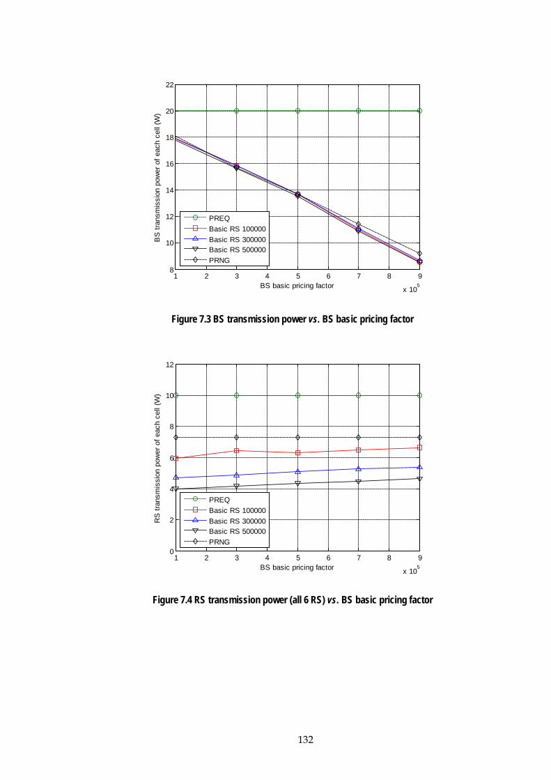
132
1 2 3 4 5 6 7 8 9
x 105
8
10
12
14
16
18
20
22
BS basic pricing factor
BS
tran
smis
sion
pow
er o
f eac
h ce
ll (W
)
PREQBasic RS 100000Basic RS 300000Basic RS 500000PRNG
Figure 7.3 BS transmission power vs. BS basic pricing factor
1 2 3 4 5 6 7 8 9
x 105
0
2
4
6
8
10
12
BS basic pricing factor
RS
tran
smis
sion
pow
er o
f eac
h ce
ll (W
)
PREQBasic RS 100000Basic RS 300000Basic RS 500000PRNG
Figure 7.4 RS transmission power (all 6 RS) vs. BS basic pricing factor

133
1 2 3 4 5 6 7 8 9
x 105
0
5
10
15
20
25
30
35
BS basic pricing factor
Tota
l tra
nsm
issi
on p
ower
of e
ach
cell
(W)
PREQBasic RS 100000Basic RS 300000Basic RS 500000PRNG
Figure 7.5 Total transmission power vs. BS basic pricing factor
The BS transmission power of LRTN and PRNG varies significantly with BSα′ , but
the RS transmission power is more or less unaffected by BSα′ , but does decrease with
increasing RSα . These conclusions are similar to those drawn for Figure 6.17 and
Figure 6.18.
At the optimum (for throughput) value for BSα′ of 510×3 and RSα of 510×3 , the BS
transmission power of LRTN is reduced from 20W to 15.8W and the RS power (for
all 6 RSs) is reduced from 10W to around 4.8W – i.e. the total power is reduced from
30W to 20.6W - a saving of nearly 32%. At the optimum (for throughput) value,
compared with PRNG, the LRTN can save 5% total transmission power.
However, that calculation optimises the throughput – if power saving is the most
significant requirement then a BSα′ can be used and the throughput kept more or
less the same as PREQ. As an example, if BSα′ is changed to 510×9 , the BS power of

134
LRTN is reduced to 8.5W and the overall power is 14.2W and the saving is 53%,
without any loss of throughput from PREQ, but with reduced fairness.
Table 7.2 Performance of LRTN relative to PREQ
Performance relative to PREQ Optimization target BSα (×105) Throughput Fairness Power
Max throughput 3 +11.5% -4.7% -32% Power saving 9 +2% -14% -53%
Summarising the performance in Table 7.2 shows that there is a tradeoff the designer
can use between power, fairness and throughput. This is also shown in Figure 7.6
where the performance gain in power saving and the reduction in fairness are
plotted against the improvement in throughput.
-20%
-10%
0%
10%
20%
30%
40%
50%
60%
0% 5% 10% 15%
Perf
orm
ance
impr
ovem
ent o
ver
PREQ
Throughput improvement over PREQ
Power
Fairness
Figure 7.6 Performance change of LRTN relative to PREQ
7.1.2 Performance Comparison between LTTN, PTNG and PTEQ
In this section the LTTN algorithm is compared with the PTNG, PTEQ algorithm
using a similar methodology as in the previous section.

135
Notice that, when both the BS and RS basic pricing factors equal zero, the system
throughput of the LTTN algorithm is still higher than in PTEQ. This is because in
LTTN, THPA is used for controlling the transmission power of the BS and RS, so
reducing co-frequency interference and hence increasing the total system throughput.
0 1 2 3 4 5 6 7
x 104
1
1.05
1.1
1.15
1.2
1.25
1.3x 10
7
BS basic pricing factor
Ave
rage
thro
ughp
ut o
f eac
h ce
ll (b
ps)
PTEQBasic RS 100000Basic RS 300000Basic RS 500000PTNG
Figure 7.7 Average throughput vs. BS basic pricing factor
0 1 2 3 4 5 6 7
x 104
0.1
0.15
0.2
0.25
0.3
0.35
0.4
0.45
0.5
0.55
0.6
BS basic pricing factor
Fairn
ess
inde
x
PTEQBasic RS 100000Basic RS 300000Basic RS 500000PTNG
Figure 7.8 User fairness vs. BS basic pricing factor

136
0 1 2 3 4 5 6 7
x 104
10
12
14
16
18
20
22
BS basic pricing factor
BS
tran
smis
sion
pow
er o
f eac
h ce
ll (W
)
PTEQBasic RS 100000Basic RS 300000Basic RS 500000PTNG
Figure 7.9 BS transmission power vs. BS basic pricing factor
0 1 2 3 4 5 6 7
x 104
0
2
4
6
8
10
12
BS basic pricing factor
RS
tran
smis
sion
pow
er o
f eac
h ce
ll (W
)
PTEQBasic RS 100000Basic RS 300000Basic RS 500000PTNG
Figure 7.10 RS transmission power vs. BS basic pricing factor

137
0 1 2 3 4 5 6 7
x 104
0
5
10
15
20
25
30
35
BS basic pricing factor
Tota
l tra
nsm
issi
on p
ower
of e
ach
cell
(W)
PTEQBasic RS 100000Basic RS 300000Basic RS 500000PTNG
Figure 7.11 Total transmission power vs. BS basic pricing factor
-60%
-40%
-20%
0%
20%
40%
60%
-10% -5% 0% 5% 10% 15%
Perf
orm
ance
impr
ovem
ent o
ver
PTEQ
Throughput improvement over PTEQ
Power
Fairness
Figure 7.12 Performance improvement of LTTN over PTEQ
Figure 7.12 shows the performance improvement of LTTN over PTEQ in the same
way that Figure 7.6 compared LRTN with PREQ. In this case with pricing values of
BSα′ = 410×1 and RSα = 510×3 (corresponding to the biggest system throughput).

138
7.1.3 Performance Comparison between LRTN and LTTN
LRTN and LTTN are different in that the channel allocation algorithm is different:
using RR and THPF respectively. Since THPF is designed to improve user fairness it
might be thought that RR might be a better solution when other factors are important.
Figure 7.13 compares the two approaches using throughput (absolute, not relative to
PREQ or PTEQ) as a common factor. It can be clearly seen that LTTN uses less power
to achieve the same throughput, or with the same fairness LTTN achieves better
throughput than LRTN. As explained earlier, this is likely to be because LTTN uses
THPF, which achieves a better tradeoff between throughput and fairness than RR.
0
0.1
0.2
0.3
0.4
0.5
0.6
0.7
0.8
0.9
1
0
5
10
15
20
25
1 1.1 1.2 1.3
Fair
ness
inde
x
Pow
er (W
)
Throughput (×107 bps)
LRTN-Power
LTTN-Power
LRTN-Fairness
LTTN-Fairness
Figure 7.13 Comparison between LRTN and LTTN based on same throughput
7.2 Performance Comparison using the NPAG-F variants
In this section the NPAG-F variants are used for the comparison using exactly the
same approach as in the previous section. For that reason detailed analysis for
comparisons of every attribute for every combination are not considered, but simply
the summary results show how, for a given throughput, each variant offers different
power saving and different fairness index. This overall comparison is shown in
Figure 7.16.

139
2 3 4 5 6 7 8
x 105
8
8.5
9
9.5
10
10.5
11x 10
6
BS basic pricing factor
Ave
rage
thro
ughp
ut o
f eac
h ce
ll (b
ps)
PREQBasic RS 200000Basic RS 600000Basic RS 800000PRNG-F
2 3 4 5 6 7 8
x 105
0.38
0.39
0.4
0.41
0.42
0.43
0.44
0.45
0.46
BS basic pricing factor
Fairn
ess
inde
x
PREQBasic RS 200000Basic RS 600000Basic RS 800000PRNG-F
a) Throughput of each cell b) Fairness index of each cell
2 3 4 5 6 7 8
x 105
10
12
14
16
18
20
22
BS basic pricing factor
BS
tran
smis
sion
pow
er o
f eac
h ce
ll (W
)
PREQBasic RS 200000Basic RS 600000Basic RS 800000PRNG-F
2 3 4 5 6 7 8
x 105
0
2
4
6
8
10
12
BS basic pricing factor
RS
tran
smis
sion
pow
er o
f eac
h ce
ll (W
)
PREQBasic RS 200000Basic RS 600000Basic RS 800000PRNG-F
c) BS transmission power of each cell d) RS transmission power of each cell
Figure 7.14 Comparison between LRTN-F, PRNG-F and PREQ

140
2 3 4 5 6 7 8
x 105
1.08
1.1
1.12
1.14
1.16
1.18
1.2x 10
7
BS basic pricing factor
Ave
rage
thro
ughp
ut o
f eac
h ce
ll (b
ps)
PTEQBasic RS 100000Basic RS 200000Basic RS 400000PTNG-F
2 3 4 5 6 7 8
x 105
0.54
0.545
0.55
0.555
0.56
0.565
BS basic pricing factor
Fairn
ess
inde
x
PTEQBasic RS 100000Basic RS 200000Basic RS 400000PTNG-F
a) Throughput of each cell b) Fairness index of each cell
2 3 4 5 6 7 8
x 105
10
12
14
16
18
20
22
BS basic pricing factor
BS
tran
smis
sion
pow
er o
f eac
h ce
ll (W
)
PTEQBasic RS 100000Basic RS 200000Basic RS 400000PTNG-F
2 3 4 5 6 7 8
x 105
7
7.5
8
8.5
9
9.5
10
10.5
11
BS basic pricing factor
RS
tran
smis
sion
pow
er o
f eac
h ce
ll (W
)
PTEQBasic RS 100000Basic RS 200000Basic RS 400000PTNG-F
c) BS transmission power of each cell d) RS transmission power of each cell
Figure 7.15 Comparison between LTTN-F, PTNG-F and PTEQ

141
0
0.1
0.2
0.3
0.4
0.5
0.6
0.7
0.8
0.9
1
0
5
10
15
20
25
30
35
0.9 1 1.1 1.2
Fair
ness
Inde
x
Pow
er (W
)
Throughput (×107 bps)
LRTN-F-Power
PREQ-Power
LTTN-F-Power
PTEQ-Power
LRTN-F-Fairness
PREQ-Fairness
LTTN-F-Fairness
PTEQ-Fairness
Figure 7.16 Comparison for the NPAG-F variants
In Figure 7.16, it is quite clear that LRTN-F and LTTN-F outperform
their ’conventional‘ counterparts in terms of requiring less power to achieve the same
throughput, yet maintain, or just surpass, the fairness index.
LTTN-F achieves higher throughput with the same power compared with LRTN-F.
And the LTTN-F achieves a higher fairness index than LRTN-F. The reason is that the
THPF and NPAG-F have the same optimisation target of user fairness. Clearly
LTTN-F is a better option than LRTN-F, just as LTTN is better than LRTN; in the next
section a comparison between LTTN and LTTN-F is considered.
7.3 Performance Comparison between LTTN and LTTN-F
Figure 7.17 shows the comparison between LTTN and LTTN-F plotted in two
different ways – against throughput and against power. It is clear from these plots
that the two variants are doing exactly what they are designed to:
• LTTN gives improved performance in terms of needing less power for the
same throughput, or indeed for achieving higher throughputs than can be
obtained with LTTN-F. This is because the NPAG algorithm is optimised for
throughput.

142
• LTTN-F gives much higher fairness index since NPAG-F is optimised for
fairness.
This demonstrates that the dominant factor in the algorithms is the NPAG – by
choosing the criteria for the game, the overall algorithm can be optimised for
those criteria.
0
0.2
0.4
0.6
0.8
1
0
5
10
15
20
25
30
1 1.05 1.1 1.15 1.2 1.25 1.3
Fair
ness
Inde
x
Pow
er (W
)
Throughput (×107 bps)
LTTN power LTTN-F-Power
LTTN-Fairness LTTN-F-Fairness
0
0.2
0.4
0.6
0.8
1
0
0.2
0.4
0.6
0.8
1
1.2
1.4
10 15 20 25 30
Fair
ness
Inde
x
Thro
ughp
ut (×
107 )
bps
Power (W)
LTTN Throughput LTTN-F Throughput
LTTN Fairness LTTN-F Fairness
a) Comparison of power and fairness vs. throughput
b) Comparison of throughput and fairness vs. power
Figure 7.17 Comparison between LTTN and LTTN-F
7.4 Summary
In this chapter, the performance of the combination of all algorithms proposed for
radio resource allocation in this thesis is analysed, including relay selection
algorithm, subchannel allocation algorithm, and power allocation algorithm. The
optimization objects for these algorithms are maximising the system throughput,
increasing the user fairness and improving the energy efficiency.
It is quite clear that the LTTN and LTTN-F versions outperform their competitors
and that the choice of NPAG or NPAG-F allows the network designer the choice of
maximising throughput (or minimizing power) or maximising user fairness. It
should be noted that the use of LTTN allows very significant (>50%) reduction in
transmission power.

143
Chapter 8 Conclusions and Future work
This thesis describes research on radio resource allocation schemes in relay based
OFDMA cellular networks; the aim of this resource management is to improve the
system throughput, user fairness and energy efficiency.
The overall conclusion is that significant power saving can be achieved without
affecting capacity but at expense of fairness; fairness can also be improved but this
requires more power. By providing different algorithms that are designed for
different optimization objects, a “tool box” of approaches is provided so the designer
or operator can choose how to optimize the network.
However, a fundamental principle is that matching the data rates on the two hops,
improves system power consumption fairness so should always be implemented.
8.1 Specific conclusions
Specific outcomes that have resulted from the work of the author and are reported in
this thesis are:
• A two-hop proportional fairness (THPF) algorithm that solves the fair
subchannel allocation between direct link users and relay link users. The
fairness seen by relay link users and by direct link users is considered, giving
a good tradeoff between system throughput and user fairness.
• A load based relay selection (LBRS) algorithm that considers the traffic load
of relay link users and direct link users for long-term user fairness. The
results reported here show that the LBRS algorithm can achieve better
fairness than the traditional relay selection algorithm in typical traffic load
distribution scenarios.
• A two-hop power allocation (THPA) algorithm that offers large energy
savings by adaptively adjusting the transmission power of the BS and RSs to
make the data rate on the two hop links of one RS match each other and

144
reduce the total transmission power of BS and RSs. The power saving can be
of the order of 30%.
• A multi-cell power allocation approach based on game theory that considers
co-channel interference. This is designed for throughput improvement and
the simulation results show that the system throughput is improved and
transmission power is reduced compared with equal power allocation. For
the NPAG-F algorithm, if user fairness is chosen as the optimisation target it
is shown that the fairness is improved greatly (over that with equal power
allocation) with only a small impact on system throughput.
• An assessment of combining the different techniques that show how the
network designer can use a combination that is optimized for either
throughput or fairness – and with the throughput version, power savings of
around 50% are achievable.
8.2 Future work
In this thesis the focus has been on RRM for relay based OFDMA networks and one
aspect that has been established is that appropriate techniques can significantly
reduce the energy consumption of the wireless part of the network while
maintaining acceptable performance for users.
Future work can be done to extend this work in the following aspects:
• All the algorithms can be modified and applied to the non-transparent
frame structure.
• The algorithms can be extended to suburban and rural scenarios .
• RRM for different QoS service catgories can be considered as an extension.
Meanwhile, there are other techniques that can improve the performance seen by
users, particularly those at the cell edge. One such technique is cooperative relay [85]
and another line of approach for further work could be on applying the principles of

145
the methods of relay selection, power allocation and channel selection to cooperative
relay networks. In particular, there has been no published work focusing on energy
efficiency in cooperative relay networks so this is an area where there is significant
potential.

146
References
[1] W. Xiaodong. "OFDM and its application to 4G," in Wireless and Optical
Communications, 2005. 14th Annual WOCC 2005. International Conference on, 2005,
pp. 69.
[2] A. Kaye, D. George, and M. Eric. "Analysis and Compensation of Bandpass
Nonlinearities for Communications," IEEE Transactions on Communications, vol.
20, pp. 965-972, Oct. 1972.
[3] IEEE C802.16x-07. "Integrated Relay Architecture for IEEE 802.16m Systems,"
Nov. 12, 2007.
[4] I. F. Akyildiz and W. Xudong. "A survey on wireless mesh networks,"
Communications Magazine, IEEE, vol. 43, pp. S23-S30, 2005.
[5] Yin and S. Alamouti. "OFDMA: A Broadband Wireless Access Technology," in
Sarnoff Symposium, IEEE, 2006, pp. 1-4.
[6] F. Kelly. "Charging and rate control for elastic traffic," European Transactions on
Telecommunications, vol. 8, pp. 33-37, Jan.1997.
[7] R. Pabst, B. H. Walke, D. C. Schultz, P. Herhold, H. Yanikomeroglu, S.
Mukherjee, H. Viswanathan, M. Lott, W. Zirwas, M. Dohler, H. Aghvami, D. D.
Falconer, and G. P. Fettweis. "Relay-based deployment concepts for wireless and
mobile broadband radio," Communications Magazine, IEEE, vol. 42, pp. 80-89,
2004.
[8] Xue Jun Li, Boon-Chong Seet, and Peter Han Joo Chong. "Multihop cellular
networks: Technology and economics,” Computer Networks, Vol. 52, pp. 1825-
1837, Jun. 2008.
[9] Jerry Sydir. "IEEE 802.16j-06/015: Harmonized Contribution on 802.16j (Mobile
Multihop Relay) Usage Models, " Sep. 2006.

147
[10] Y. Wang, X. Qu, T. Wu, and B. Liu. "Power Allocation and Subcarrier Pairing
Algorithm for Regenerative OFDM Relay System," in Vehicular Technology
Conference, 2007. VTC2007-Spring. IEEE, 2007, pp. 2727-2731.
[11] K.J.Ray Liu, Ahmed K.Sadek, Weifeng Su and Andres Kwasinski. Cooperative
communications and networking. Cambridge: Cambridge University Press, 2009,
pp. 122-126.
[12] V. Genc, S. Murphy, Y. Yang, and J. Murphy. "IEEE 802.16J relay-based wireless
access networks: an overview," Wireless Communications, IEEE, vol. 15, pp. 56-63,
2008.
[13] Abdulkareem Adinoyi, Lars Berlemann, John Boyer, etc. "IST-2003-507581
WINNER D3.2: Description of identified new relay based radio network
deployment concepts and first assessment by comparison against benchmarks of
well known deployment concepts using enhanced radio interface technologies. "
Internet: www.ist-winner.org, Feb. 2005.
[14] IEEE 802.16's Relay Task Group, Internet: http://wirelessman.org/relay, web
date [Dec. 4.2009].
[15] Wireless World Initiative New Radio (WINNER), Internet: www.ist-winner.org,
[Sep. 10.2009].
[16] Hui Liu and Guoqing Li. OFDM-Based Broadband Wireless Networks: Design and
Optimization. Hoboken, New Jersey: John Wiley & Sons, 2005, pp. 13-29.
[17] R.R Moisier and R.G. Clabaugh. "Kineplex, a bandwidth-efficient binary
transmission system,” AIEE Transactions. vol. 76, pp. 723-728, Jan.1958.
[18] R. Chang and R. Gibby. "A Theoretical Study of Performance of an Orthogonal
Multiplexing Data Transmission Scheme," Communication Technology, IEEE
Transactions on, vol. 16, pp. 529-540, Aug. 1968.

148
[19] Chang Robert W. "Orthogonal Frequency Multiplex Data Transmission System,"
US Patent Publication number: 3488445. Jan. 1970.
[20] S.B. Weinstein, and P.M.Ebert, "Data transmission by frequency division
multiplexing using the discrete Fourier transform," Communications, IEEE
Transactions on, Vol.COM-19, pp. 628-634, Oct. 1971.
[21] Hirosaki B. "An orthogonally multiplexed QAM System Using Discrete Fourier
Transform," Communications, IEEE Transactions on vol. COM-29, pp. 982-989, Jul.
1981.
[22] ETS 300 401, "Digital audio broadcasting (DAB); DAB to mobile, portable and
fixed receivers," Internet: http://portal.etsi.org/broadcast/dab.asp, Feb, 1995.
[23] Peled A, Ruiz A. "Frequency domain data transmission using reduced
computational complexity algorithms," in Proceeding ICASSP, 1980: pp.964-967.
[24] Harri Holma, Antti Toskala. LTE for UMTS - OFDMA and SC-FDMA Based Radio
Access. UK: John Wiley & Sons Ltd, 2009, pp 69-71.
[25] J. Jiho and L. Kwang Bok, "Transmit power adaptation for multiuser OFDM
systems," in Selected Areas in Communications, IEEE Journal on, vol. 21, pp. 171-178,
2003.
[26] A. J. Goldsmith and C. Soon-Ghee, "Variable-rate variable-power MQAM for
fading channels," Communications, IEEE Transactions on, vol. 45, pp. 1218-1230,
1997.
[27] IEEE 802.16j-06/026r4, "Baseline Document for Draft Standard for Local and
Metropolitan Area Networks part 16: Air Interface for Fixed and Mobile
Broadband Wireless Access Systems – Multihop Relay Specification, " Jun. 2007.

149
[28] IEEE Draft Std P802.16j "Draft Standard for Local and Metropolitan Area
Networks--Part 16: Air Interface for Fixed and Mobile Broadband Wireless
Access Systems-Multihop Relay Specification," Aug. 2007.
[29] P. Won-Hyoung and B. Saewoong, "WLC25-3: Resource Management Policies
for Fixed Relays in Cellular Networks," in Global Telecommunications Conference,
2006. GLOBECOM '06. IEEE, 2006, pp. 1-5.
[30] IEEE 80216j-06_013r3, "Multi-hop Relay System Evaluation Methodology
(Channel Model and Performance Metric)," Feb. 2007.
[31] 3GPP R1-050676. "Text Proposal: Simulation Assumptions and Evaluation for
EUTRA, " June, 2005.
[32] 3GPP R1-050623. "Text proposal: Principles for the Evolved UTRA, " June 2005.
[33] 3GPP2 CR1002 V1.0. "CDMA2000 Evaluation Methodology, " December 2004.
[34] L. Jemin, P. Sungsoo, W. Hano, and H. Daesik, "QoS-guaranteed Transmission
Scheme Selection for OFDMA Multi-hop Cellular Networks," in Communications,
2007. ICC '07. IEEE International Conference on, 2007, pp. 4587-4591.
[35] K. Doppler, H. Xiaoben, C. Wijting, and A. Sorri, "Adaptive Soft Reuse for Relay
Enhanced Cells," in Vehicular Technology Conference, 2007. VTC2007-Spring. IEEE
65th, 2007, pp. 758-762.
[36] H. Lei, R. Mengtian, W. Lan, X. Yisheng, and E. Schulz, "Resource Scheduling for
OFDMA/TDD Based Relay Enhanced Cellular Networks," in Wireless
Communications and Networking Conference, 2007.WCNC 2007. IEEE, 2007, pp.
1544-1548.
[37] IEEE 802.16.3c-01/29r4, "Channel Models for Fixed Wireless Applications." July,
2001.

150
[38] 3GPP R1-091320, “Radio Characteristics of the ITU Test Environments and
Deployment Scenarios.” March, 2009.
[39] S. A. AlQahtani and A. S. Mahmoud. "Dynamic radio resource allocation for 3G
and beyond mobile wireless networks," Computer Communications, vol. 30, pp.41-
51, 2006.
[40] V. Sreng, H. Yanikomeroglu, and D. D. Falconer, "Relayer selection strategies in
cellular networks with peer-to-peer relaying," in Vehicular Technology Conference,
2003. VTC 2003-Fall. 2003 IEEE 58th, 2003, pp. 1949-1953.
[41] IEEE C802.16e -04/152, "Time first vs. Frequency first allocations in OFDMA
mode," Jun. 2004.
[42] Mohsen Guizani. Wireless communications systems and networks, New York:
Springer, 2004, pp.102.
[43] Mischa Schwartz, Mobile wireless communications, Cambridge: Cambridge
University Press, 2005, pp. 21.
[44] Sanam Sadr, Alagan Anpalagan, and Kaamran Raahemifar, "Suboptimal Rate
Adaptive Resource Allocation for Downlink OFDMA Systems," International
Journal of Vehicular Technology, vol. 2009, pp. 10, 2009.
[45] L. Venturino, N. Prasad, and W. Xiaodong, "Coordinated Scheduling and Power
Allocation in Downlink Multicell OFDMA Networks," Vehicular Technology, IEEE
Transactions on, vol. 58, pp. 2835-2848, 2009.
[46] Z. Tiankui, Z. Zhimin, F. Chunyan, C. Jie, and S. Lianbo, "Uplink power
allocation for interference coordination in multi-cell OFDM systems," in
Communications and Networking in China, 2008, pp. 716-720.

151
[47] Z. Dawy, S. Davidovic, and I. Oikonomidis. "Coverage and capacity
enhancement of CDMA cellular systems via multihop transmission," in Global
Telecommunications Conference, IEEE, 2003, pp. 1147-1151.
[48] V. Sreng, H. Yanikomeroglu, and D. Falconer. "Coverage enhancement through
two-hop relaying in cellular radio systems," in Wireless Communications and
Networking Conference. WCNC2002. IEEE, 2002, pp. 881-885.
[49] A. A. N. A. Kusuma and L. L. H. Andrew. "Minimum power routing for
multihop cellular networks," in Global Telecommunications Conference, 2002. IEEE,
2002, pp. 37-41.
[50] T. Rouse, S. McLaughlin, and I. Band. "Congestion-based routing strategies in
multihop TDD-CDMA networks," Selected Areas in Communications, IEEE Journal
on, vol. 23, pp. 668-681, 2005.
[51] I. Krikidis and J. C. Belfiore. "Three Scheduling Schemes for Amplify-and-
Forward Relay Environments," Communications Letters, IEEE, vol. 11, pp. 414-416,
2007.
[52] N. Truman Chiu-Yam and Y. Wei. "Joint optimization of relay strategies and
resource allocations in cooperative cellular networks," Selected Areas in
Communications, IEEE Journal on, vol. 25, pp. 328-339, 2007.
[53] Y. N. Yao-Nan Lee, J. C. Jung-Chieh Chen, Y. C. Yeong-Cheng Wang, and J. T.
Jiunn-Tsair Chen. "A Novel Distributed Scheduling Algorithm for Downlink
Relay Networks," Wireless Communications, IEEE Transactions on, vol. 6, pp. 1985-
1991, 2007.
[54] I. Hammerstrom, M. Kuhn, and A. Wittneben. "Channel adaptive scheduling for
cooperative relay networks," in Vehicular Technology Conference, 2004. VTC2004-
Fall. IEEE 60th, 2004, pp. 2784-2788.

152
[55] Y. Liu, R. Hoshyar, X. Yang, and R. Tafazolli. "Integrated Radio Resource
Allocation for Multihop Cellular Networks With Fixed Relay Stations," Selected
Areas in Communications, IEEE Journal on, vol. 24, pp. 2137-2146, 2006.
[56] L. Xin, E. K. P. Chong, and N. B. Shroff. "Optimal opportunistic scheduling in
wireless networks," in Vehicular Technology Conference, 2003. VTC 2003-Fall. IEEE
58th, 2003, pp. 1417-1421.
[57] K. Hoon and H. Youngnam. "An Opportunistic Channel Quality Feedback
Scheme for Proportional Fair Scheduling," Communications Letters, IEEE, vol. 11,
pp. 501-503, Jun. 2007.
[58] M. HU, J.S. Zhang, "Opportunistic Multi-Access: Multiuser Diversity, Relay-
Aided Opportunistic Scheduling," Mobile Networks and Applications, Volume 9,
pp. 435–444, Nov. 2004.
[59] G. Li, and H. Liu, "Resource Allocation for OFDMA Relay Networks With
Fairness Constraints," Selected Areas in communications, IEEE Journal on, vol. 24,
pp. 2061-2069, Nov.2006.
[60] B. Chisung, and C. Dong-Ho, "Fairness-Aware Adaptive Resource Allocation
Scheme in Multihop OFDMA Systems," Communications Letters, IEEE, vol. 11, pp.
134-136, Feb. 2007.
[61] M. O. Hasna and M. S. Alouini, "Optimal power allocation for relayed
transmissions over Rayleigh-fading channels," Wireless Communications, IEEE
Transactions on, vol. 3, pp. 1999-2004, Nov. 2004.
[62] Q. Zhang, J. Zhang, C. Shao, Y. Wang, P. Zhang, and R. Hu, "Power allocation
for regenerative relay channel with Rayleigh fading," in Vehicular Technology
Conference, VTC 2004-Spring. 2004 IEEE 59th, 2004, pp. 1167-1171 Vol.2.

153
[63] J. Zhang, Q. Zhang, C. Shao, Y. Wang, P. Zhang, and Z. Zhang, "Adaptive
optimal transmit power allocation for two-hop non-regenerative wireless
relaying system," in Vehicular Technology Conference, 2004. VTC 2004-Spring. 2004
IEEE 59th, 2004, pp. 1213-1217 Vol.2.
[64] G.-D. Yu, Z.-Y. Zhang, Y. Chen, S. Chen, and P.-l. Qiu, "Power allocation for non-
regenerative OFDM relaying channels," in Wireless Communications, Networking
and Mobile Computing, 2005. Proceedings. 2005 International Conference on, 2005, pp.
185-188.
[65] I. Hammerstrom and A. Wittneben, "On the Optimal Power Allocation for
Nonregenerative OFDM Relay Links," in Communications, 2006. ICC '06. IEEE
International Conference on, 2006, pp. 4463-4468.
[66] J. Hee-jin and M. Cheol, "Capacity of Multiuser Diversity with Cooperative
Relaying in Wireless Networks," Communications Letters, IEEE, vol. 12, pp. 752-
754, 2008.
[67] Lin Xiao, Laurie Cuthbert. "Improving fairness in relay-based access networks,"
in ACM MSWIM 2008, Nov. 2008, pp. 18-22.
[68] J. Eatwell, M. Milgate, and P. Newman, Macmillan. "Game Theory," in The New
Palgrave, A Dictionary of Economics, Vol 2, London and Basingstoke: Palgrave
Macmillan, 1987, pp. 460-482.
[69] John von Neumann, and Oskar Morgenstern. Theory of Games and Economic
Behavior. Princeton University Press, 1944.
[70] A.Alcaide, J.M.Estevez-Tapiador, J.C.Hernandez Castro, and A.Ribagorda. "An
extended model of rational exchange based on dynamic games of imperfect
information," Emerging Trends in Information and Communication Security,
Vol.3995, pp.396-408, June, 2006.

154
[71] A.Alcaide, J.M.Estevez-Tapiador, J.C.Hernandez Castro, and A.Ribagorda.
"Bayesian rational exchange," International Journal of Information Security. Volume
7, pp. 85-100, Sep. 2008.
[72] E.Palomar, A.Alcaide, J.M.Estevez-Tapiador, J.C.Hernandez Castro. "Bayesian
analysis of secure P2P sharing protocols," Proceeding of the Information Security
Workshop, LNCS, vol.4805, pp. 1701-1717, Nov. 2007.
[73] A.B.MacKenzie, L.Dasilva, and W.Tranter. Game Theory for Wireless Engineers.
San Rafael, CA: Morgan and Claypool Publishers, 2006.
[74] E.Altman, T.Boulogne, R.EI Azouzi, T. Jimenez, and L.Wyneter. "A survey on
networking games in telecommunications," Computer and Operations Research,
Volume 33, pp.286-311, Feb.2006.
[75] L.Buttyan and J.P. Hubaux. Security and Cooperation in Wireless Networks.
Cambridge, U.K: Cambridge University Press, 2007.
[76] M.Felegyhazi and J.P. Hubaux. "Game theory in wireless networks: A tutorial,"
in EPFL technical report: LCA-REPORT-2006-002, Feb. 2006.
[77] Klaus Ritzberger. Foundations of non-cooperative game theory. New York, USA:
Oxford university press, 2002, pp. 7.
[78] D. Goodman and N. Mandayam. "Power control for wireless data," Personal
Communications, IEEE, vol. 7, pp. 48-54, Apr. 2000.
[79] Saraydar C U, Mandayam N, Goodman D. Efficient Power Control via Pricing in
Wireless Data Networks. Communications, IEEE Transactions on, Vol. 50, pp. 291-
303, 2002.
[80] K. Hojoong and L. Byeong Gi, "Distributed Resource Allocation through
Noncooperative Game Approach in Multi-cell OFDMA Systems," in
Communications, 2006. IEEE International Conference on, 2006, pp. 4345-4350.

155
[81] Y. Xinmin, W. Tong, H. Jing, and W. Ying, "A Non-Cooperative Game Approach
for Distributed Power Allocation in Multi-Cell OFDMA-Relay Networks," in
Vehicular Technology Conference, 2008. IEEE, 2008, pp. 1920-1924.
[82] Kiyosi Ito, Encyclopedic Dictionary of Mathematics: The Mathematical Society of Japan,
Second edition, Publisher: The MIT Press, Cambridge, USA, 1993, pp. 331, pp.
1614.
[83] Akira Takayama, Mathematical economics, Second edition, Cambridge, UK:
Cambridge University Press, 1985, pp. 113.
[84] 3GPP R1-061487. “Uplink Interference Mitigation via Power Control," May. 2006.
[85] IEEE C80216j-06_006r1, “Cooperative Relay in IEEE 802.16j MMR)," May. 2006.