radio network feedback to improve tcp utilization over
TRANSCRIPT

Radio Network Feedback to Improve TCP Utilization over Wireless Links
I N É S C A B R E R A M O L E R O
Master's Degree ProjectStockholm, Sweden 2005
IR-RT-EX-0502


Abstract
During the past years, TCP has proven to be unable to perform properly inwireless environments, with high bandwidth-delay product paths and band-width variation. The recent development of advanced 3G networks and ser-vices makes it necessary to find ways to improve TCP’s efficiency and resourceutilization, as well as improve the user’s experience and reduce latency times.
This report presents a proxy-based solution called Radio Network Feed-back, which aims at improving the performance of TCP over 3G networks.The solution proposes the use of a proxy to split the TCP connection betweenremote servers and mobile terminals. It manages to adapt the parametersof the connection to the wireless link characteristics, by making use of theinformation provided by the Radio Network Controller. The results are eval-uated through a set of simulations that compare the performance of RadioNetwork Feedback to that of TCP.
The simulation results show that the Radio Network Feedback solutiongreatly improves the link utilization when used over wireless links, comparedto TCP. It manages to reduce latency times, especially during Slow Startand after and outage. It also succeeds in maintaining reduced buffer sizes,and properly adapts to varying network conditions.
i

ii ABSTRACT

Contents
Abstract i
1 Introduction 11.1 Background . . . . . . . . . . . . . . . . . . . . . . . . . . . . 1
1.1.1 The Transmission Control Protocol (TCP) . . . . . . . 21.1.2 Introduction to Third Generation Networks . . . . . . 5
1.2 Problem definition . . . . . . . . . . . . . . . . . . . . . . . . 61.3 Objective . . . . . . . . . . . . . . . . . . . . . . . . . . . . . 71.4 Solution approach . . . . . . . . . . . . . . . . . . . . . . . . . 71.5 Limitations . . . . . . . . . . . . . . . . . . . . . . . . . . . . 71.6 Organization . . . . . . . . . . . . . . . . . . . . . . . . . . . 8
2 Problems with TCP 92.1 Problems with wireless networks . . . . . . . . . . . . . . . . . 92.2 Problems with 3G networks . . . . . . . . . . . . . . . . . . . 14
3 Improvements to the TCP protocol 153.1 Classification of solutions . . . . . . . . . . . . . . . . . . . . . 153.2 Overview of proposed solutions . . . . . . . . . . . . . . . . . 173.3 Desired characteristics of a solution for UMTS . . . . . . . . . 24
4 The HSDPA channel 254.1 Introduction to the HSDPA concept . . . . . . . . . . . . . . 254.2 HSDPA in detail . . . . . . . . . . . . . . . . . . . . . . . . . 26
4.2.1 Adaptive Modulation and Coding . . . . . . . . . . . . 264.2.2 Hybrid Automatic Repeat Request . . . . . . . . . . . 274.2.3 Packet Scheduling . . . . . . . . . . . . . . . . . . . . . 27
4.3 Conclusions, outlook and implications . . . . . . . . . . . . . . 28
5 The Radio Network Feedback solution 295.1 Architecture . . . . . . . . . . . . . . . . . . . . . . . . . . . . 30
iii

iv CONTENTS
5.2 Scenario . . . . . . . . . . . . . . . . . . . . . . . . . . . . . . 325.3 Detailed description of the algorithm . . . . . . . . . . . . . . 33
5.3.1 Proxy-Terminal control . . . . . . . . . . . . . . . . . . 345.3.2 Proxy-Server control . . . . . . . . . . . . . . . . . . . 46
5.4 Proxy control model . . . . . . . . . . . . . . . . . . . . . . . 485.4.1 Overview of the queue control algorithm . . . . . . . . 485.4.2 Analysis of the closed loop system . . . . . . . . . . . . 51
6 Simulations and results 536.1 Tools and modules . . . . . . . . . . . . . . . . . . . . . . . . 546.2 General performance . . . . . . . . . . . . . . . . . . . . . . . 55
6.2.1 Connection startup . . . . . . . . . . . . . . . . . . . . 556.2.2 Delay changes . . . . . . . . . . . . . . . . . . . . . . . 566.2.3 Algorithm reliability . . . . . . . . . . . . . . . . . . . 576.2.4 Outages . . . . . . . . . . . . . . . . . . . . . . . . . . 59
6.3 Use Cases . . . . . . . . . . . . . . . . . . . . . . . . . . . . . 616.3.1 Use case 1: FTP with small files . . . . . . . . . . . . . 616.3.2 Use case 2: Web browsing . . . . . . . . . . . . . . . . 666.3.3 Use case 3: FTP with large files . . . . . . . . . . . . . 69
7 Conclusions and outlook 75
Realimentacion de la Red Radio para mejorarla utilizacion de recursos de TCP en redes
inalambricas
Autor: Ines Cabrera Molero
Tutor: Karl Henrik Johansson
Institucion: Grupo de Control Automatico, Departamento de Senales, Sen-sores y Sistemas (S3), KTH, Estocolmo (Suecia)
Lectura: Miercoles 26 de Enero de 2005 en el Departamento de Senales,Sensores y Sistemas (S3), KTH, Estocolmo (Suecia)
Este proyecto consiste en el diseno, analisis y simulacion de una solucionllamada “Radio Network Feedback” (o “Realimentacion de la Red Radio”)para redes moviles de tercera generacion, a fin de mejorar las prestaciones delprotocolo de transporte TCP. La solucion esta basada en la introduccion deun proxy, a fin de mejorar la utilizacion de recursos y maximizar la velocidadde transmision de datos, y a la vez obtener un tiempo de respuesta reducido.
El objetivo es reducir el impacto en la eficiencia del protocolo de trans-porte de ciertas caracterısticas de los enlaces inalambricos, como la variaciontemporal del ancho de banda disponible y el retardo extremo a extremo,ası como las desconexiones esporadicas de los terminales moviles. Para ello,se asume que la red de acceso esta bien dimensionada, y que todos los erroresdel canal se recuperan a nivel de enlace (lo que se traduce en ancho de banday retardo variable).
La idea basica es separar la conexion TCP entre un servidor remoto y unterminal movil en dos conexiones independientes con un proxy intermedio, elcual se encarga de la gestion de ambas conexiones y de la adaptacion de losparametros de TCP a fin de obtener la maxima utilizacion de recursos. Parallevar a cabo dicha adaptacion, el proxy utiliza parte de la informacion acercade las caracterısticas fısicas del enlace entre la estacion base y el terminalmovil, que se halla disponible en el controlador (RNC) situado en la red de

acceso radio del operador. Esta informacion (ancho de banda disponible enel canal y longitud de la cola en el controlador) es transmitida al proxy en undatagrama UDP, y se utiliza en los algoritmos de adaptacion para controlar,entre otras cosas, la velocidad de transmision.
En primer lugar, se identificaron los principales problemas del protocoloTCP en redes inalambricas, y se realizo un estudio en profundidad de lasdiferentes soluciones propuestas previamente. La mayorıa de las solucionesanteriores se centra en algunos de los problemas, pero apenas ninguna cubretodos ellos, y en cualquier caso requieren la modificacion de los extremos dela comunicacion (servidores y/o terminales). La arquitectura presentada eneste proyecto intenta solucionar todos los problemas en uno, sin necesidad demodificar el codigo de los extremos. Esto es posible si el proxy implementaun protocolo que consiste en una modificacion de TCP, capaz de adaptarla velocidad de transmision a las caracterısticas fısicas variables del enlaceradio. Los algoritmos de adaptacion se basan en informacion fiable aportadapor la red misma, en vez de en estimaciones realizadas en los extremos dela conexion, como ocurre en las versiones de TCP disponibles actualmente.Ademas, se realizo un breve estudio de las caracterısticas del canal HSDPArecientemente introducido en sistemas celulares UMTS.
Las mejoras en las prestaciones pueden ser analizadas desde el punto devista de los operadores, ası como en terminos de grado de satisfaccion delos usuarios. Estos ultimos requieren mejoras en el tiempo de respuesta delsistema, ası como reduccion del tiempo de espera para recibir los archivosdemandados, ambas caracterısticas necesarias para la introduccion de servi-cios interactivos y de tiempo real. Por otra parte, los operadores requieren unuso eficiente de los caros y escasos recursos radio, ası como obtener sistemasescalables y con capacidad para soportar un numero elevado de usuarios.
A fin de comparar las prestaciones de la solucion disenada con las de TCP(en este caso, la version mas usada, TCP Reno), se llevo a cabo una seriede simulaciones utilizando el simulador Network Simulator 2 (ns2). Se anal-izo tanto las prestaciones generales (eficiencia al comienzo de la transmision,porcentaje de ancho de banda utilizado frente al ancho de banda disponible,retardo, memoria requerida, etc.), como respuesta en situaciones practicas(descarga de ficheros de varios tamanos desde un servidor remoto, y accesoweb). Los resultados de las simulaciones demuestran que es posible incremen-tar la utilizacion de los recursos disponibles y la eficiencia de las conexionesTCP, ası como reducir las necesidades de memoria, la longitud de las colasen elementos intermedios de la red y los retardos extremo a extremo. Lasolucion presentada supera con creces la eficiencia de TCP Reno, reduce lalatencia en la fase inicial de la conexion TCP (“Slow Start”), y se adapta conexito a variaciones temporales tanto del ancho de banda como del retardo.

Finalmente, el uso de un proxy situado en la red del operador UMTSproporciona a los operadors un control completo sobre los algoritmos deadaptacion, y les permite asegurar tanto que los recursos son utilizados efi-cientemente, como que las caracterısticas de los servicios que ofrecen cumplenlas condiciones requeridas. Por otra parte, el proxy facilita la gestion y man-tenimiento del sistema, ya que todas las modificaciones y mejoras quedanreducidas a un solo elemento (el proxy en sı). Por otra parte, esta solucionse basa unicamente en la introduccion de un elemento intermedio, el cualrealiza todas las operaciones de forma transparente. Esto evita la necesidadde modificar los servidores remotos o los terminales moviles, lo que facilita suintroduccion y reduce los costes tanto para usuarios como para operadores.

Chapter 1
Introduction
1.1 Background
During the last years, interconnections between computers have grown inimportance, and nowadays it is difficult to think of an isolated machine as itcould be done some years ago. Networks (and especially the Internet) playa major role in todays communication, and there is a growing trend towardsmobility, what brings new challenges and needs. Extensive research needsto be carried out to keep pace with the changing environment and moredemanding requirements. These include higher bandwidth for faster accessto contents, lower response time, delay constraints for real-time communica-tion and mobility issues. Older protocols and technologies are beginning tobecome obsolete as they are unable to keep up with the new requirements.Therefore, there is a real need to improve the current ones and tailor themto the new situation, or move towards newer and more specific ones.
One important matter of concern is the development of mobile networks,which bring up different problems from wired ones and require very specificsolutions. Wireless networks normally present higher delays and high errorrates, something not dealt with by traditional wired protocols. In fact, oneof the main problems that wireless links have to face is that many of theassumptions made by wired protocols are not valid in the wireless domain.However, it is highly desirable to have interoperating (if not the same) pro-tocols, and to find a way to connect machines independently of their locationor their access media. Thus it is a good idea to try to adapt to differentsituations from the network, in a way that is totally transparent, if possible,to the endpoints of the connection.
1

2 CHAPTER 1. INTRODUCTION
Application
Transport
Network
Link
Physical
HTTP, FTP...
TCP, UDP
IP
Ethernet, PPP...
Application
Transport
Network
Link
Physical
HTTP, FTP...
TCP, UDP...
IP
Ethernet, PPP...
Network
Link
Physical
IP
Ethernet, PPP...
R
Figure 1.1: Internet protocol stack
1.1.1 The Transmission Control Protocol (TCP)
TCP [1] is the most widely used transport protocol on the Internet. It pro-vides a connection-oriented and reliable end-to-end communication betweentwo endpoints, and ensures an error-free, in-order delivery of data. In spite ofbeing connection-oriented, all the connection state resides on the endpoints,so intermediate network elements, in principle, do not maintain connectionstate and are oblivious to the TCP connection itself. Thus, all the connectionmanagement and control has to be performed at the endpoints. This impliesthat most of the information they need must be inferred from estimationsand measurements, and that the performance of TCP strongly depends onthe accuracy of them.
In order to provide reliable delivery, TCP breaks the application data intosmaller chunks called ”segments”, and uses sequence numbers to facilitate theordering and reassembling of packets at the destination. Sequence numbersare used to retransmit any lost or corrupted segment, as well as to performTCP’s advanced congestion control algorithms. It uses cumulative acknowl-edgements (acks) to inform of correctly received data, and an error-recoverymechanism for reliable data transfer that lies between go-back-N and Selec-tive Repeat. Acks from the destination reflect the highest in-order sequencenumber received, although out-of-order received packets can be buffered andacknowledged later. This reduces the number of retransmissions of properlyreceived data.

1.1. BACKGROUND 3
The Internet protocol stack is represented in figure 1.1. It shows the layersinvolved in the indirect (i.e., through a router) communication between twoendpoints. According to the layer separation, intermediate network elementsdo not need to include any other level above the Network level. Therefore,transport protocols such as TCP are end-to-end, in the sense that TCPsegments are encapsulated into IP packets, and forwarded to the destination.TCP headers are not examined by intermediate routers. For a more detailedexplanation of the Internet protocol stack and layers, see [2].
TCP includes mechanisms both for flow and congestion control. Flowcontrol is achieved by having the receiver inform of its current receive windowrecvwnd, what gives an idea of how much free buffer space is available at thedestination. Congestion control is performed through the use of a differentwindow at the sender, the congestion window cwnd, whose size is increased ordecreased depending on the network conditions. Finally, the sending windowwnd of a TCP entity should never exceed any of these two limits, so it isdetermined by the minimum of both,
wnd = min{recvwnd, cwnd}
The size of the window wnd represents the maximum amount of unac-knowledged data that the sender can handle, thus it sets a limit on thesending rate R. Once a TCP entity has sent wnd bytes, it needs to receive atleast one ack in order to be able to continue sending, therefore it can transmita maximum of wnd bytes per round-trip time (RTT ). This way, the sendingrate can be easily controlled by modifying wnd, and it can be expressed as
R =wnd
RTT
The main objective of TCP’s Congestion Control algorithm is to have theTCP sender limit its own sending rate when it faces congestion on the path tothe destination. It is a window-based control algorithm, where as expressedabove, the size of the window has a direct relation to the rate at which thesender injects data into the network. The basic idea is to allow the senderincrease its rate while there are available resources, and to decrease it whencongestion is perceived. This behavior is achieved by increasing or decreasingcwnd accordingly, as represented in figure 1.2. The algorithm comprises threemain parts: Slow Start, Congestion Avoidance, and Reaction to congestion.
• The Slow Start phase takes place at the beginning of the connection.During this phase, the sender is trying to reach the maximum band-width available to the connection as fast as possible. Therefore, the

4 CHAPTER 1. INTRODUCTION
2
4
6
8
10
12
14
16
18C
onge
stio
n w
indo
w (p
kts)
1 2 3 4 5 6 7 8 9 10 11 12 13 14 15 16
threshold
threshold
threshold
Slow Start
Congestion Avoidance
3 dupacks
timeout
Time (RTTs)
Figure 1.2: TCP’s Congestion Window in Reno implementation
cwnd is initialized to one segment (hence the name ”Slow Start”), butits size is doubled every RTT, so it grows exponentially fast. This phaseends when the value of cwnd reaches a predefined threshold, which de-termines the point at which the Congestion Avoidance phase shouldbegin.
• The aim of the Congestion Avoidance phase is to gently probe the loadof the network, by increasing cwnd by one packet per RTT. This is thedesirable behavior when its value corresponds to a sending rate closeto the the maximum bandwidth that the network can provide (i.e, theconnection is operating on the limits of congestion). Thus, when thesender is transmitting at a rate close to the network limit, it tries toincrease its rate by increasing its window slowly. The sender will remainin this phase until it faces a congestion event (represented by a timeoutor the arrival of three duplicated acks).
• When the sender comes up against a congestion indication, it assumesthat congestion has occurred, and that the best idea is to drasticallydecrease the sending rate. The way this reduction is performed dependson the TCP version. The first implementations of TCP used to followthe Tahoe algorithm, where a timeout is not considered different fromthree duplicated acks. Both congestion indications result in the sendershrinking cwnd to one segment, setting the value of the threshold to half

1.1. BACKGROUND 5
the value it had at the moment congestion was detected, and going backto slow start. Newer TCP versions (such as TCP Reno) consider thisalgorithm too conservative, and they distinguish a loss indication dueto a timeout from the occurrence of three duplicated acks. A timeoutcauses the TCP Reno sender behave in the same way as the previousTahoe implementations, but the reception of three duplicated acks areconsidered as a warning rather than an indication of congestion. Insuch case both the threshold and cwnd are set to half the value of theprevious threshold. Thus, the sending rate is reduced by half, and thesender stays in Congestion Avoidance instead of going back to SlowStart.
1.1.2 Introduction to Third Generation Networks
A wireless link is an interconnection of two or more devices that communicateto each other via the air interface instead of cables. In general, any networkmay be described as “wireless” if at least one of its links is a wireless link.
Third Generation (3G) mobile networks can be considered a particularcase of wireless networks, where wireless links are used to connect the mobilenodes to the operators wired backbone. 3G networks are the next generationof mobile cellular networks, and their origin is an initiative of the Interna-tional Telecommunications Union (ITU). The main objective is to providehigh-speed and high-bandwidth (up to 10 Mbps in theory) wireless servicesto support a wide range of advanced applications, specially tailored for mo-bile personal communication (such as telephony, paging, messaging, Internetaccess and broadband data).
UMTS stands for “Universal Mobile Telecommunications System”. It isone of the main third generation mobile systems, developed by ETSI withinthe IMT-2000 framework proposed by the ITU. It is probably the most ap-propriate choice to evolve to 3G from Second Generation GSM cellular net-works, and for that reason it was the preferred option in Europe. Currently,the Third Generation Partnership Project, formed by a cooperation of stan-dards organizations (ARIB, CWTS, ETSI, T1, TTA and TTC), is in chargeof developing UMTS technical specifications. UMTS systems have alreadybeen deployed in most European countries, although new and advanced ter-minals, as well as many specifications, are still under development.
Wideband Code Division Multiple Access (WCDMA) is a technology forwideband digital radio communications that was selected for UMTS. It is a3G access technology that increases data transmission rates in GSM systems.
6 CHAPTER 1. INTRODUCTION
1.2 Problem definition
Although TCP’s Congestion Control algorithm has proven effective for manyyears, it has been shown that it lacks the ability to adapt to situations thatdiffer from the ones for which it was originally designed. TCP is prepared towork in wired networks, with reasonably low delays, and with low link errorrates. In such cases, data is seldom lost or corrupted due to link errors, andthe main cause of packet loss is data being discarded in congested routers. Forthat reason, TCP always considers a loss indication as a sing of congestion,and takes action accordingly.
However, there is an increasing number of situations where this assump-tion is no longer valid. Wireless links present high Bit Error Rates (BER),and it is undesirable for a protocol to react to link errors (also called ’ran-dom losses’) the same way it reacts to congestion indications. TCP is unableto distinguish a loss due to congestion (where decreasing the sending rateis necessary to alleviate the congested link) from a random loss, where re-ducing the rate is not only useless, but it is counterproductive as well. Inparticular, and due to the physical characteristics of the air interface, wirelesslinks are likely to present many consecutive losses. Such situation causes theTCP sender to cut repeatedly the sending rate by half, leading to a seriousdegradation of performance.
Moreover, the mobility of terminals brings up the problem of disconnec-tions. Shadowing and fading of the radio signal may cause the destinationto be temporarily unreachable, what leads to the TCP sender stopping thetransmission. The lack of a mechanism to inform the TCP sender that thedestination is reachable again introduces extra delays, that increase the re-sponse time of the connection.
Third Generation (3G) cellular networks are a particular case of wirelessnetworks, where random losses at the wireless portion of the network arerecovered through the use of robust and strongly reliable link layer protocols.However, this error correction and recovering also has shortcomings, as itincreases the link delay as well as the delay variance. Moreover, the factthat the network capacity is shared among all the users in a particular cellintroduces significant bandwidth variations to which TCP is unable to adapt.
To sum up, the result of using TCP without further improvement overnetworks that contain wireless links is a decrease in the average link utiliza-tion, an increase in the latency of the connection, and in general an overallunder-utilization of the -often scarce- wireless resources.
1.3. OBJECTIVE 7
1.3 Objective
The aim of this thesis is to design, analyze and simulate a proxy-based solu-tion, called Radio Network Feedback (RNF), to improve the performance ofTCP over Third Generation cellular networks. It extends the RNF solutionproposed in [3]. It is supposed to improve the resource utilization and max-imize the transmission rates while maintaining the shortest response timepossible, by taking advantage of feedback information provided by the net-work itself. It should add on the performance improvements brought by therecently released High Speed Downlink Packet Access (HSDPA), which pro-vides broadband support for downlink packet-based traffic. It should alsoovercome the problems that TCP connections face over wireless links.
1.4 Solution approach
The main idea is to split the connection between a server and a mobileuser through the introduction of a proxy, which terminates both connectionsand is capable of adapting its parameters to get the best out of the availableresources. The proxy takes advantage of the fact that most of the informationthat a TCP sender needs to infer in order to perform congestion control, isalready known by the radio network. In that case, it can be transmittedto the proxy in order to feed its adaptation algorithm, as is the case of thebandwidth available for a determined connection, or the network load.
1.5 Limitations
The Radio Network Feedback solution focuses on the problems introducedby variable bandwidth and delay, wireless link utilization and sporadic dis-connections of mobile terminals. It does not address other problems suchas congestion or dimensioning of the wired part of the UMTS network, norcongestion on parts that do not belong to the 3G network (i.e, between theproxy and the remote servers). It assumes that all the possible link errors arerecovered by the link level protocols, and that the 3G backbone is properlydimensioned. However, the improved TCP implementation in the proxy stillhas the basic TCP functionalities, thus it would be able to work (althoughwithout any added improvements on the basic TCP algorithms) in the faceof such situations.
8 CHAPTER 1. INTRODUCTION
1.6 Organization
The rest of this report is organized as follows: in Chapter 2 the main problemswith TCP in wireless and 3G networks are described and analyzed in depth,while an overview of the proposed improvements and alternatives to TCP forwireless links is presented in Chapter 3.
The concept of High Speed Downlink Packet Access and its main featuresare introduced in Chapter 4. Chapter 5 presents and describes in detail theproposed Radio Network Feedback solution, along with a brief theoreticalanalysis of its behavior when implemented in the proxy.
The performance of the proposed solution is tested through a set of simu-lations that are described in Chapter 6. There, the results of the simulationsare presented, analyzed and compared. Finally, Chapter 7 draws some con-clusions and proposes some guidelines for future work.

Chapter 2
Problems with TCP
When used in networks that contain wireless links, TCP presents many prob-lems that need to be dealt with. Some of them are related to wireless networksin general, while others are specific to Third Generation networks.
The performance of a TCP connection is heavily dependent on the Bandwidth-Delay Product (BDP) of the path to the destination, also called “pipe ca-pacity”. The BDP is defined as the product of the transmission rate R andthe round-trip time RTT,
BDP = R · RTT (2.1)
and measures the amount of unacknowledged data that the TCP sendermust handle in order to maintain the pipe full, i.e., the required buffer spaceat both the sender and the receiver to permanently fill the TCP pipe. Theutilization of the available resources of the path is closely related both to thisfigure and the sending window wnd of the TCP sender. If the sender’s wndis smaller than the BDP, there are determined moments where the window isfull and prevents the sender from transmitting more data, although at leastone packet could be transmitted. This situation is translated into a decreasein the link utilization, as it can be observed in figure 2.2, something highlyundesirable when the resources are scarce and expensive. On the other hand,figure 2.1 shows a situation where wnd is at least equal to the path BDP,therefore the sender is permanently injecting packets into the link.
2.1 Problems with wireless networks
The first and straightforward consequence of using a wireless link as part ofthe path to a destination is an increase in the total delay of the path, mainlydue to the contribution of propagation and link-level error recovering delays,
9

10 CHAPTER 2. PROBLEMS WITH TCP
SenderReceiver
ack ack ack ack ack ack ack ack ack
Figure 2.1: Full pipe with 100% link utilization
SenderReceiver
ack ack ack ack ack ack
Figure 2.2: Under-utilization of resources on a pipe
if present. When combined with high offered bandwidth (something commonin wireless networks), the result is a high Bandwidth-Delay Product path.A necessary condition for an adequate link utilization is to have the senderuse a big enough wnd value (at least equal to the pipe capacity). However,TCP uses 16 bits to codify the receive window (recvwnd) that is sent backto the sender, what leads to a maximum window of 65KBytes. This valuemight be significantly smaller that some of the existing BDP values, hencethe performance of TCP could be seriously damaged.
Another direct consequence of having a big BDP is that it introducesthe need to use big windows, and the combination of high delays and widewindows may have a negative effect on the TCP retransmission mechanism.TCP needs at least one round-trip time to detect a packet loss (through atimeout or three duplicated acks), but it is unable to figure out if the restof the packets that it has sent during this time have been received correctly.This leads to the retransmission of many already received packets, whatreduces the goodput (i.e., the rate of actual data successfully transmittedfrom the sender to the receiver) of the connection. If the sender is usinga big window, the number of retransmissions of properly received packetsincreases, hence the goodput is further reduced. Moreover, the use of big

2.1. PROBLEMS WITH WIRELESS NETWORKS 11
SR SR
ack
ack
a) High link delay b) Low link delay
Figure 2.3: Higher link delay gives lower link utilization during slow start
windows reduces the accuracy of TCP’s RTT measurement mechanism, andcan cause problems if the sequence number of the TCP data packets wrapsaround.
A particularly harmful result of high delay paths is the increase in thelatency time during the Slow Start phase. As it has been described before,during Slow Start the sender begins the transmission with the lowest ratepossible, that corresponds to a cwnd of 1. The value of cwnd is then doubledevery round-trip time (it is increased in one packet per ack received), whatimplies an exponential growth of the sending rate. However, a high value ofthe RTT may significantly slow down the growth of cwnd, as it may introduceremarkably high waiting times between the sending of one packet and thereception of its ack. This increases considerably the time it takes to theconnection to reach a reasonably high sending rate. This situation especiallyaffects short file transfers (such as web browsing), which spend most of thetime in Slow Start, due to the fact that the initial Slow Start latency has asubstantial impact on the total file transfer time. Figure 2.3 compares twosituations with different link delays, where time progress is represented inthe vertical axis. It can be observed that in case a) it takes longer to reachfull link utilization, due to the fact that the link delay is higher than in caseb).

12 CHAPTER 2. PROBLEMS WITH TCP
100
Tran
smis
sion
rate
(Kbi
ts/s
)
1 2 3 4 5 6 7 8 9 10 11 12 13 14 15 16
Bandwidth under-utilization
Time (seconds)
200
300
400
500
600
700
800
900 3 dupacks 3 dupacks
3 dupacks
timeout
Available bandwidthSender's transmission rate
Figure 2.4: Bandwidth under-utilization due to random losses
A different but not less important problem that arises when TCP is usedon wireless networks is the high BER of the links. TCP was originally de-signed to operate in wired environments, where segment loss is mainly causedby packets being dropped at intermediate routers, due to network congestion.However, wireless links are characterized by a high probability of randomlosses, mostly due to physical degradation of the radio signal (such as shad-owing and fading).
Such losses in principle do not depend on the transmission rate, and theyare not caused by congestion in intermediate network elements. On the otherhand, TCP is unable to distinguish a packet loss due to a congested networkfrom a random loss, so it considers any kind of loss as a sign of congestion. Asa direct result, the occurrence of a random loss on a wireless link causes theTCP sender invoke the usual congestion avoidance mechanisms, what leads toa drastic reduction of the transmission rate. While this conservative measureis appropriate to alleviate congestion, it has no effect on the occurrence ofrandom losses, it reduces the link utilization and degrades the overall TCPperformance.
Figure 2.4 shows a situation where, due to random link errors, the senderis not always transmitting at the maximum rate offered by the link. Randomlosses cause the sender to invoke TCP’s Congestion Control mechanisms, onthe assumption that a loss is a sign of congestion, and halve its sending rate.The grey area represents the amount of underutilized bandwidth, i.e., the

2.1. PROBLEMS WITH WIRELESS NETWORKS 13
difference between the available bandwidth and the actual sending rate.
Moreover, if the wireless channel is in deep fade for a significant amountof time, errors are like to appear in bursts, what causes the TCP sender todecrease its sending rate repeatedly, leading to a severe under-utilization ofthe available resources.
Another matter of concern is the effect of disconnections, a common situ-ation when the wireless link is the last hop to the destination. Disconnectionsare closely related to the mobility of terminals. Physical obstacles and lim-ited coverage may cause a terminal to be out of reach for a significant amountof time, what is detected at the sender by the occurrence of many timeouts.This situation makes the TCP sender stop the transmission of packets, andconsider the destination as unreachable.
However, after reconnection, TCP lacks a mechanism to inform the senderthat the destination is reachable again. The only way for the sender to detectthis is to periodically send a probe (i.e., one single packet sent towards thereceiver), and hope to get a response. This mechanism is called “ExponentialBackoff”, as the time between the probes increases exponentially. The senderstays in Exponential Backoff until it receives a response from the receiver,when the destination is considered reachable again, and the transmission isresumed.
The main problem with this mechanism is that it is not possible to im-mediately detect that a terminal is reachable again when it reconnects, asthe sender has to wait for a timer to expire to send a probe. In an unfavor-able situation, the terminal may reconnect right after a probe has been lost.Then, the sender will need to wait for a whole interval until is it allowedto send a new probe, in order to detect the reconnection and resume thedata transmission. This can introduce an extra delay up to 64 seconds (i.e.,the maximum interval in the exponential backoff), what might significantlyincrease the total transmission time. Figure 2.5 shows a situation where achannel recovers after an outage, but it remains idle for some time as thesender cannot send a probe until the Exponential Backoff timer expires. Assoon as the probe is sent, the transmission is resumed.
Another problem inherent to TCP is its sawtooth behavior, due to TCP’sCongestion Avoidance algorithm. TCP increases its congestion window untilthere is a drop, when the transmission rate is cut to half. Therefore, TCPhas a tendency to put as much data in the network as possible, filling thequeues to the limit. Long queues imply higher delays and lower responsetimes, and the straightforward solution (to provide the routers with biggerbuffers) can lead to scalability problems.

14 CHAPTER 2. PROBLEMS WITH TCP
R
S
Exponential Backoff
OutageDest. Reachable Dest. Reachable
Idle Channel
Figure 2.5: Exponential Backoff upon a disconnection
2.2 Problems with 3G networks
As 3G networks can be considered a particular case of wireless networks,where the wireless part corresponds to the links that connect the mobileterminals to the 3G backbone, both of them share similar characteristics.However, 3G networks overcome some of the problems of wireless networkspresent, at the expense of bandwidth and delay variation.
One of the main differences is that the link layer at the wireless portion ofthe network is very reliable in UMTS. The impact of random losses on TCPperformance has encouraged the use of extensive local retransmissions. TheRadio Link Control (RLC) layer can correct or recover most of the losses,thanks to a combination of Forward Error Correction (FEC) and AutomaticRepeat Request (ARQ) techniques, so it can be assumed that packet lossesare only caused by buffer overflows or disconnections. Thus, the problemof TCP mistakenly invoking Congestion Avoidance in presence of randomlosses is overcome. However, this techniques also have shortcomings, as theheavy link layer protocols introduce an overhead that reduces the availablebandwidth and increase the delay variance.
However, the problem of disconnections is still present, and it is especiallyworsened as mobility is an inherent feature of 3G terminals.

Chapter 3
Improvements to the TCPprotocol
The problems that TCP faces when used over wireless links, presented inchapter 2, have been known for a long time, hence a lot of research hasbeen carried out in this field. There are many different solutions that try toovercome these weaknesses, all of them having their advantages and short-comings. Some solutions need support from the network, while others as-sume that only the endpoints are responsible for the efficiency of the TCPconnection. In general, the best solution is the one that best adapts to theenvironment and makes use of the available information and support.
3.1 Classification of solutions
The modifications of the TCP protocol can be classified in two ways. Oneway takes into consideration how and where the adaptation is performed:end-to-end, link layer and split connection. Another option is to classifythem according to which TCP problem they address.
End-to-end solutions assume that it is not possible to rely on the networkin order to improve the performance of the transport protocol. In such cases,the endpoints are responsible of performing the necessary changes to ensurea good adaptation, and they must be aware of the problems of TCP. Themain advantage is that these solutions can be used in any situation, as theydo not depend on the underlying layers. However, the code of either thesender or the receiver (or even both) must be modified, which might be ashortcoming in many cases.
On the contrary, link layer solutions manage to improve TCP’s perfor-mance from the network itself. These alternatives rely on determined network
15

16 CHAPTER 3. IMPROVEMENTS TO THE TCP PROTOCOL
Classification Solution
TCP’s Window Scale optionTCP’s Timestamps optionTCP’s Selective AcknowledgementsTCP Vegas
End-to-end TCP WestwoodTCP’s Increased Initial WindowsFast StartSmooth StartAdaptive StartFreeze-TCP
E2E + Network support Explicit Bandwidth Notification (EBN)
Automatic Repeat Request (ARQ)Forward Error Correction (FEC)Snoop protocol
Link layer Ack RegulatorWindow RegulatorPerformance Enhancing Proxy (PEP)Explicit Window Adaptation (EWA)Fuzzy Explicit Window Adaptation (FEWA)
Split connection M-TCPRadio Network Feedback
Table 3.1: Classification of proposed TCP solutions

3.2. OVERVIEW OF PROPOSED SOLUTIONS 17
elements, which collaborate at link level in order to reduce the effects of thewireless link. In this case, it is the network (instead of the terminals) thatmust be aware of the problems of TCP over wireless links. These solutionsreduce and hide the problems from the transport layer, so the endpoints donot need to be aware of the problem. Link layer solutions make the wirelesslink appear as a higher quality link, but with reduced effective bandwidth.The main advantage is that the code in terminals and servers does not needto be modified. However, some of these solutions (such as link layer re-transmissions and extensive error correction) are not able to overcome theproblems of disconnections caused by wireless shadowing and fading.
Finally, split-connection solutions manage to completely hide the wirelesslink from the wired portion of the network. They achieve so by terminatingthe TCP connection at the base station, and establishing another connectionfrom the base station to the wireless nodes. The transport protocol used inthe latter can be TCP, a modification of TCP, or any other suitable protocol.These solutions are said to be more efficient than the previous ones, and theendpoints do not need to be aware of the adaptation. However, there is aneed to translate from one protocol to the other at the base station, with theresulting overhead.
On the other hand, all these solutions can also be classified accordingto which TCP problem they address. This way, some solutions focus onthe problems caused by long, fat pipes (such as the Window Scale option,Selective Acknowledgements, and TCP Timestamps). Others try to solve theproblems of congestion avoidance in high error rate paths (such as many TCPmodifications like TCP Vegas and TCP Westwood, or the Snoop protocol).There are also proposed solutions that try to improve Slow Start performance(such as Astart or Fast Start). The problem of outages and disconnectionsis addressed by solutions like Freeze-TCP and M-TCP, while others dealwith bandwidth and delay variation (such as Ack Regulator and WindowRegulator). All these solutions are further explained in the following section.
3.2 Overview of proposed solutions
The solutions concerning high bandwidth-delay product often propose theintroduction of special TCP options in order to deal with such problems:
• RFC 1072 [4] defines a new option called Window Scale, which solvesthe problem of window size limitation explained in section 2.1. Thisoption introduces a 16-bit scaling factor to be applied by the sender tothe receive window, hence the window value can be scaled from 16 to 32
18 CHAPTER 3. IMPROVEMENTS TO THE TCP PROTOCOL
bits. This approach solves the window limitation problem, but havinghuge windows involve other problems that must also be addressed.
• As explained in section 2.1, using bigger windows might introduce otherproblems like sequence number wrap-around, not very accurate RTTmeasurements, and problems caused by packets from previous connec-tions. RFC 1185 [5] proposes the use of TCP timestamps to solve allthese problems at once. Timestamps are sent inside data packets by theTCP sender, and they are echoed by the receiver in the returning acks.These echoed 32-bit timestamps can be used to measure the Round-Trip Time, as well as to distinguish new packets from old ones (in casethe sequence number has wrapped around). RFC 1323 [6] refines theWindow Scale and Timestamps options, and includes an algorithm toprotect against wrapped sequence numbers (PAWS).
• Finally, the performance of TCP might be degraded when multiplepackets are lost from one window of data. This problem is worsenedwhen using big windows, i.e., when the Window Scale option is beingused. RFC 2018 [7] proposes a selective (instead of cumulative) ac-knowledgement mechanism (SACK), based on the introduction of twonew TCP options. The SACK mechanism allows the receiver to ac-knowledge non-contiguous blocks of correctly received data, somethingthat cumulative acks cannot achieve. This prevents the sender from re-transmitting packets that have been received, but in the wrong order.
Section 2.1 introduced the problems caused by high BER links. TCP’sCongestion Avoidance mechanism reacts to random packet losses as if theywere a sign of congestion, excessively reducing the throughput. Some TCPmodifications have been proposed in order to achieve a more effective band-width utilization, while others are performed at link level:
• TCP Vegas [8] is a new version of TCP, with a modified CongestionAvoidance algorithm. It tries to avoid the oscillatory behavior of theTCP window. While a basic TCP version linearly increases its con-gestion window until there is a timeout or three duplicated acks (theso-called additive increase-multiplicative decrease), TCP Vegas usesthe difference between the expected and actual rates to estimate theavailable bandwidth in the network. It computes an estimation of theactual queue length at the bottleneck, and updates its congestion win-dow to ensure that the queue length is kept within a determined range.TCP Vegas’ algorithm is called “additive increase-additive decrease”.In summary, it increases or decreases its cwnd value in order to keep at

3.2. OVERVIEW OF PROPOSED SOLUTIONS 19
least α packets but no more than β packets in the intermediate queues.The main advantage of TCP Vegas is that, while previous TCP versionsincrease the queue length towards queue overflow, TCP Vegas managesto keep a small queue size. Therefore, it avoids queue overflows andunnecessary reduction of the transmission rate. However, it might findsome problems with rerouting, and Vegas connections may starve whenthey compete with TCP Reno.
• TCP Westwood [9] is also a sender-side modification of TCP Reno. Ittries to avoid the drastic reduction in the transmission rate caused byrandom link errors. It computes an end-to-end bandwidth estimationby monitoring the rate of returning acks, and uses this estimation tocompute the Slow Start Threshold and congestion window after a con-gestion indication (“Faster Recovery”). Adjusting the window to theestimated available bandwidth makes TCP Westwood more robust towireless losses, as the transmission rate is not reduced to half, but itis adapted to the most recent bandwidth estimation instead. As de-fined in [10], TCP Westwood modification affects only the CongestionAvoidance algorithm (“additive increase-adaptive decrease”), but theSlow Start phase remains unchanged, as well as the linear increase ofthe window between two congestion episodes. Some performance anal-ysis carried out in [11] and [12] show that TCP Westwood manages toobtain a fair share of the bandwidth when it coexists with other West-wood connections, and it is friendly to other TCP implementations.
• A wide range of link layer solutions include error correction (suchas Forward Error Correction, FEC) and retransmission mechanisms(such as Automatic Repeat Request, ARQ). These protocols manageto achieve a high link reliability, at the expense of bandwidth. Theyare the preferred solution in UMTS networks, which make use of ex-tensive local retransmissions in order to recover most of the wirelesslosses. However, none of them can help in the face of disconnectionsand outages, so in such cases the TCP sender still times out and entersExponential Backoff.
• The Snoop protocol [13] is a TCP-aware link layer protocol. The Snoopagent resides in the base station, and monitors every TCP packet thatpasses through the connection. It keeps a cache of TCP packets, andit also keeps track of which packets have been acknowledged by thereceiver. It detects duplicated acks and timeouts, and performs localretransmissions of lost packets. Its main objective is to locally recoverrandom losses, and hide the effects of the wireless link from the TCP

20 CHAPTER 3. IMPROVEMENTS TO THE TCP PROTOCOL
sender. This way, it prevents the sender from mistakenly invokingCongestion Avoidance algorithms in the face of random wireless loss,which do not reflect a congested network. The main advantage of Snoopis that is has proven to be highly efficient, and that code modificationsare only needed at the base stations, thus both servers and receivers canbe kept unchanged. However, Snoop does not bring any improvementin absence of wireless losses, and it is not able to cope with outagesand disconnections.
Slow Start latency might significantly contribute to the total transmissiontime of a TCP file transfer. The performance of TCP during Slow Start canbe seriously worsened if the RTT of the path is high. For this reason, manysolutions have been proposed to improve TCP’s performance on connectionstartup:
• RFC 3390 [14] introduces the possibility to increase the initial windowof the TCP connection up to four packets. This measure is supposed toreduce the transmission time for connections transmitting only a smallamount of data (short-lived TCP connections). Moreover, it speedsup the growth of the sending rate in high bandwidth-delay paths. Themain disadvantage is that it increases the burstiness of the TCP traffic,but this is most likely to be a problem in already congested networks.Moreover, bursts of 3-4 packets are already common in TCP, so in-creasing the initial window should not be an added problem.
• The performance of TCP on connection startup is analyzed in [15],along with the importance of setting an adequate Slow Start Threshold.Too low thresholds relative to the BDP cause a premature exit of theSlow Start phase, which reduces the growth of the sending rate andleads to poor startup utilization. On the contrary, too high thresholdsmight cause many packet drops and retransmissions. There are manyproposed solutions to choose an adequate threshold, like Fast Start[16], which uses cached values of the threshold and cwnd from recentconnections. On the other hand, Smooth Start [17] reduces the growthof cwnd around values close to the threshold, in order to guarantee asoft transition between Slow Start and Congestion Avoidance, and toavoid possible packets drops and bottleneck congestion.
• Adaptive Start [15] (ASTART) uses the bandwidth estimation com-puted in TCP Westwood, based on the ack stream, to dynamicallyupdate the value of the Slow Start Threshold. ASTART increases theduration of the Slow Start phase if the bandwidth-delay product is high,
3.2. OVERVIEW OF PROPOSED SOLUTIONS 21
and switches to Congestion Avoidance when the transmission rate isclose to the link bandwidth. As the previous solutions, it improvesstartup performance in high BDP paths, but the sender code needs tobe modified.
The problem of disconnections was introduced in section 2.1, and it wasfurther explained in section 2.2. Outages and disconnections might intro-duce a significant delay, and must be properly dealt with. There are someapproaches that try to reduce the effect of TCP’s Exponential Backoff algo-rithm:
• M-TCP [18] proposes a split-connection solution, which uses a band-width management module that resides at the Radio Network Con-troller (RNC). The main feature of M-TCP is that it allows to freezethe TCP sender during a disconnection, and resume the transmission atfull speed when the mobile terminal reconnects. This effect is achievedby controlling the size of the receive window, sent back to the sender inevery ack, and by setting it to zero during a disconnection. This eventforces the sender into “persist mode”, and although the transmissionis paused, the sender does not time out and it does not close its cwnd.Upon terminal reconnection, the M-TCP module at the RNC sends awindow update to the sender (through one ack), and the transmissionis immediately resumed, without the need to wait for the ExponentialBackoff algorithm to time out.
• Freeze-TCP [19] follows a similar approach, but instead of split-connection,it is completely end-to-end. Unlike M-TCP, it does not need an inter-mediary. In Freeze-TCP, it is the terminal itself (instead of the RNC)that shrinks its receive window when the radio signal is weakened, thusforcing the sender into persist mode. Upon reconnection, the termi-nal is in charge of sending three duplicated acks in order to awake thesender and resume the transmission, in a way that is very similar tothe M-TCP approach. The main advantage over M-TCP is that Freeze-TCP does not need an intermediary, which could become a bottleneck.However, the complexity of the receiver increases, as it must monitorthe radio signal and react to disconnections.
Some solutions focus on the problems caused by bandwidth and delayvariation, as well as limited buffer space in the bottlenecks. These solutionsare especially efficient in the case of UMTS networks, where random lossesare recovered at link level:
22 CHAPTER 3. IMPROVEMENTS TO THE TCP PROTOCOL
• The Ack Regulator solution [20] runs in an intermediate bottlenecknetwork element, such as the RNC in the case of UMTS networks,or a congested router in a general case. It determines the amount offree buffer space at the bottleneck, and monitors the arrival rate ofpackets. Then, it controls the acks sent back to the sender, in order toregulate its transmission rate, and prevent buffer overflows. The mainadvantage of the ack regulator is that no modification is needed at theendpoints. Moreover, it performs well for long-lived TCP connections.However, it does not address the performance of short-lived flows (suchas HTTP), and some estimation problems might reduce the sender’stransmission rate more than necessary.
• The Window Regulator approach [21] is based on the ack regulatorexplained above. It manages to improve the performance of TCP forany buffer size at the bottleneck. It tries to obtain a similar effectas the Ack Regulator through the modification of the receive windowvalue in the acks sent from the receiver back to the sender, as wellas an ack buffer in order to absorb channel variations. The WindowRegulator tries to ensure that there is always at least one packet in thebuffer, in order to prevent buffer underflows. On the other hand, itensures that the amount of buffered data is kept under a limit, in orderto prevent buffer overflows. Maintaining the queue length within thedesired limits is achieved by controlling the sender’s transmission rate.The sender’s rate is controlled by dynamically computing the adequatereceive window value, and setting this value in the receiver’s acks. Themain limitation of this approach is that it needs to have both datapackets and acks following the same path, or at least traversing thesame bottleneck router, where the Window Regulator module runs.
• A similar approach to the Ack Regulator is presented in [22]. Thissolution proposes the use of Performance Enhancing Proxies (PEPs)at the edges of unfriendly networks, in order to control the TCP flowspassing through them. The idea is that high link delays make TCPflows less responsive to bandwidth variations. PEPs are in charge ofmonitoring the available bandwidth to the flows, and manipulating theacks to speed up or slow down the TCP senders. A PEP can send a“premature” ack in order to simulate a lower RTT, and make the TCPsender respond faster. PEPs must also recover any lost packets inthe path between themselves and the destinations, thus preventing thesender from invoking Congestion Avoidance algorithms in the presenceof random losses.

3.2. OVERVIEW OF PROPOSED SOLUTIONS 23
• The Explicit Window Adaptation (EWA) [23] follows a very similarapproach. It also controls the sender’s transmission rate through themodification of the receive window in the receiver’s acks. However, thecomputation of the receive window value is different, and follows a log-arithmic expression. Like the previous solutions, the EWA approachalso needs symmetrical routing, and might have problems if the bot-tleneck router is lowly loaded for a long period of time. Moreover, itcannot adequately deal with bursty traffic.
• The Fuzzy Explicit Window Adaptation (FEWA) [24] tries to overcomethe problems of the EWA approach, by introducing a Fuzzy controllerto improve the algorithm. Its working principles are the same, and thecontrol is performed through the modification of the receive window.It also needs symmetrical routing, but it manages to solve many of theproblems related to the EWA solution.
• While TCP Vegas and Westwood try to obtain a good estimation of theavailable bandwidth to adapt the transmission rate, the Early Band-width Notification (EBN) architecture [25] manages to improve TCPperformance by improving the bandwidth estimation with support fromintermediate nodes. The idea is to have an intermediate router measurethe bandwidth available to a TCP flow, and feedback this informationto the TCP sender. The modified TCP sender (TCP-EBN) then ad-justs its cwnd to adapt its sending rate to this bandwidth. In order tomake the TCP sender receive the instantaneous bandwidth feedback,the EBN router encodes the measured value in the data packets thattraverse it towards the destination, and the sender receives this informa-tion in the acks. EBN is especially effective for continuous bandwidthvariation, and it does not need symmetrical routing.
Finally, some solutions have been proposed in order to address many ofthese problems at the same time. In general, these solutions are based on alink layer mechanism, combined with some other mechanism than relies onthe support of the network. This is the case of the Radio Network Feedback(RNF) technique introduced in [3]. The RNF mechanism proposes the useof an intermediate network element, namely a proxy, which splits the TCPconnection in two. The proxy receives explicit notifications of the radiolink parameters (i.e., the bandwidth) from the Radio Network Controller viaUDP, and adapts the TCP connection parameters in order to achieve thehighest link utilization.

24 CHAPTER 3. IMPROVEMENTS TO THE TCP PROTOCOL
3.3 Desired characteristics of a solution for
UMTS
As it was introduced in section 2.2, UMTS networks make use of very reliablelink layer protocols, such as Automatic Repeat Request and Forward ErrorCorrection. Thus, it can be assumed that the problem of random losses iscompletely overcome. However, there are many other problems that must beaddressed in order to improve TCP performance in UMTS networks:
• The solution must prevent the TCP sender from mistakenly invokingCongestion Avoidance mechanisms, unless there is actually a conges-tion situation.
• It must properly detect and react to handoffs, disconnections and out-ages. This includes preventing the TCP sender from timing out andshrinking the congestion window in those situations.
• For the sake of efficiency, scalability and reduced response times, itshould limit the amount of buffered data in intermediate network ele-ments, such as the RNC.
• In order to ensure high link utilization, it must make an efficient useof the bandwidth resources, and avoid reducing the transmission ratein situations where it is not strictly necessary. This especially includesconnection startup performance.
• According to the wireless link characteristics, it must be able to copewith variable bandwidth and delay, and achieve a good performanceeven in the face of these events.
• Although it is not a must, it is desirable that the solution providescompatibility, i.e., it should be able to interoperate with existent serversand terminals, without the need to modify the code in any of them.

Chapter 4
The HSDPA channel
4.1 Introduction to the HSDPA concept
During the last years, the volume of IP traffic has experienced a substantialincrease. The same situation is most likely to apply to mobile networks,due to the development of IP-based mobile services, as well as the increasein the use of IP person-to-person communication. Packet-switched traffic islikely to overtake circuit-switched traffic, and 3G operators will need to dealwith this situation. There is a real need for a solution that ensures a highutilization of the available resources as well as high data rates, and that canbe easily deployed while being backwards compatible.
The High Speed Downlink Packet Access (HSDPA) is a packet-baseddata service used in W-CDMA that was included in the 3GPP Release 5 [26].It is specially tailored for asymmetrical and bursty packet-oriented traffic,while being a low cost solution to upgrade existing infrastructure. One ofits main features is that it will allow operators to support a higher num-ber of users with improved downlink data rates. It can co-exist in the samecarrier as previous releases, and in fact it is an enhancement of the UMTSdownlink shared channel. The HSDPA channel can theoretically provide upto 10.8 Mbps (and in practice up to 2 Mbps) by employing time and codemultiplexing, which is especially efficient for bursty flows. Recent perfor-mance evaluations have shown that HSDPA is able to increase the spectralefficiency1 gain in 50-100% compared to previous releases, by taking advan-tage of new and more specific link level retransmission strategies and packetscheduling.
1The spectral efficiency of a digital signal is given by the number of bits of data persecond that can be supported by each hertz of band. It can also be estimated as thethroughput of the connection divided by the total available bandwidth.
25

26 CHAPTER 4. THE HSDPA CHANNEL
RBS
User1
User2
User3
Shared Downlink Channel (HS-DSCH)
UE
Figure 4.1: Flow multiplexing in HSDPA
4.2 HSDPA in detail
The main idea behind the HSDPA channel is to share one single downlinkdata channel between all the users, along with many modifications that makeit especially effective for packet-based communication. These include timemultiplexing with a short transmission interval, what facilitates monitoringof the radio channel conditions, Adaptive Modulation and Coding (AMC),hybrid ARQ and multicode transmission, among others. Moreover, many ofthe functions are moved from the Radio Network Controller (RNC) to thebase station (RBS), where there is an easy access to air interface measure-ments. The HSDPA specification introduces a downlink transport channel,denominated High-Speed Physical Downlink Shared Channel (HS-PDSCH).It also introduces other common and dedicated signaling channels that areused to deliver the data, receive channel quality and network feedback andmanage the scheduling. The HS-PDSCH is divided in 2ms slots that are usedto transmit data to all the users in the cell. This time multiplexing is espe-cially efficient for bursty or packet-oriented flows, in which the data streamis not continuous. Sharing the channel between different users reduces theimpact of silences, which substantially reduces efficiency in dedicated chan-nels.
4.2.1 Adaptive Modulation and Coding
One of the main characteristics of 3G wireless channels is that, due totime varying physical conditions, the Signal to Interference and Noise Ra-tio (SINR) can vary up to 40 dB. 3G systems modify the characteristicsof the signal transmitted to user equipments to compensate for such varia-tions, through a link adaptation process. Link adaptation is normally basedon modifications and control of the transmission power, such as WCDMA’s

4.2. HSDPA IN DETAIL 27
Fast Power Control [27]. However, power control has been shown to be lim-ited by interference problems between users, and it is unable to properlyreduce the power for users close to the base station. Therefore, HSDPA triesto improve the link adaptation by modifying the modulation scheme to af-fect the transmission rate, while keeping the transmission power constant,through the use of Adaptive Modulation and Coding (AMC). In AMC, thebase station determines the Modulation and Coding Scheme (MCS) to usetowards a particular user, based on power measurements, network load, avail-able resources and Channel Quality Indications (CQI). CQIs are periodicallysent by the user equipment, and they reflect the MCS level that the termi-nal is able to support under the current channel conditions. According toperformance evaluations in [28], this adaptive modulation control can covera range of variation of 20dB, and it can be further expanded through the useof multi-coding.
4.2.2 Hybrid Automatic Repeat Request
Transmitting at the highest rates to improve spectral efficiency involves asignificant increase in the block error rate. Thus, there is a need for anadvanced link layer mechanism to reduce the delay introduced by multipleretransmissions of corrupted packets, and to increase the retransmission ef-ficiency. In HSDPA, the retransmission scheme used is Hybrid AutomaticRepeat Request (H-ARQ), that combines forward error correcting with astop-and-wait (SAW) protocol. To reduce the waiting times in SAW, manychannels are used to ensure reliable transmission of different packets in paral-lel. A N-channel SAW has a good tradeoff for obtained throughput, memoryrequirements and complexity. Moreover, the MAC layer resides at the basestation, thus reducing the delay introduced by every retransmission. How-ever, as it is stated in [29], the throughput gain that H-ARQ can providedepends mainly on the performance of the Adaptive Modulation and Codingfunction.
4.2.3 Packet Scheduling
As the HSDPA concept takes advantage of a shared downlink channel foruser data, the packet scheduling method is a critical point, and it is the mainresponsible of ensuring a high channel utilization and spectral efficiency. Thepacket scheduling functions in HSDPA are used to determine the utilizationof the time slots, and they are located at the RBS, thus facilitating advancedscheduling techniques and immediate decisions. Scheduling is based on bothchannel quality and terminal capability, and it can be further affected by

28 CHAPTER 4. THE HSDPA CHANNEL
Quality of Service (QoS) decisions. Different strategies can be adopted, froma simple round-robin scheme to more complex and advanced methods, suchas the Proportional Fair Packet Scheduler.
A simple round-robin scheme is represented in figure 4.1. Many differentflows are multiplexed in time in order to share a single downlink channel.The information about how to extract the data sent to a determined UserEquipment is provided through a shared control channel (HS-SCCH), alongwith other control signaling.
4.3 Conclusions, outlook and implications
The HSDPA solution is a promising alternative to deal with future needs in3G networks. It improves the system capacity and optimizes the networkto decrease the cost per bit, allowing more users per carrier. It increasesremarkably the spectral efficiency and throughput, is cost-effective and fa-cilitates flexible scheduling strategies. In addition, from the users point ofview, it increases the peak data rate and reduces latency, service responsetime, and variance in delay.
However, in order to take full advantage of this solution, there is a need tofind a way to overcome the problems that TCP faces on wireless links. Thefact that the bandwidth of the downlink data channel is shared among allusers implies high bandwidth variation. As one user is assigned a determinedamount of bandwidth depending on the number of users of the cell (as theyall compete for the resources), the available bandwidth for a connection isaffected by the number of users entering and leaving the cell. According tothe simulations and results, the Radio Network Feedback solution seems tobe a way to overcome this problem, as well as many others that current TCPversions over cannot solve.
Chapter 5
The Radio Network Feedbacksolution
The Radio Network Feedback (RNF) mechanism is a proxy-based solution,that is intended to overcome most of the problems that TCP faces overUMTS networks. Most of its functionality resides in a proxy that is situatedin the UMTS backbone, and that acts as an intermediary between the mobileterminals and the content providers. The proxy aims to reduce latency andSlow Start time, improve the wireless link utilization and reduce the bufferneeds in intermediate elements of the network. It is in principle designedfor asymmetric downlink traffic, such as web browsing and ftp file transfer,but it could easily be extended to deal with person-to-person symmetriccommunication.
The proxy implements a modified version of TCP, in order to adapt itsbehavior to the special characteristics of the wireless environment, somethingthat current TCP versions have failed in achieving. It splits the TCP con-nection in two, in order to hide the wireless link from the wired servers, andadapts the connection parameters in a way that is completely transparent tothe endpoints.
The use of proxies has been criticized for being a potential bottleneck,and for being prone to scalability problems. However, the introduction of aproxy allows to solve the wireless problem locally, and without the need toinvolve the endpoints. A careful design and implementation could also helpto make it scalable. One of the shortcomings is that, as it is in essence asplit-connection approach with two independent TCP connections, it is notpossible to maintain end-to-end semantics.
The proxy manages to fulfil the requirements defined in section 3.3. Beingespecially tailored to a UMTS scenario, it relies on the RLC layer to ensurea reliable transmission of packets. According to the pipe sizes currently used
29
30 CHAPTER 5. THE RADIO NETWORK FEEDBACK SOLUTION
RBSUE
RBS
UE
UE
RNC SGSN GGSN
VLR HLR
IP Network
Proxy
Packet-switched Core NetworkUTRAN
Figure 5.1: Simplified UMTS network architecture
in UMTS, it does not need to address window size limitation problems, soTCP’s Selective Acknowledgements, Window Scale and Timestamps optionsare not needed.
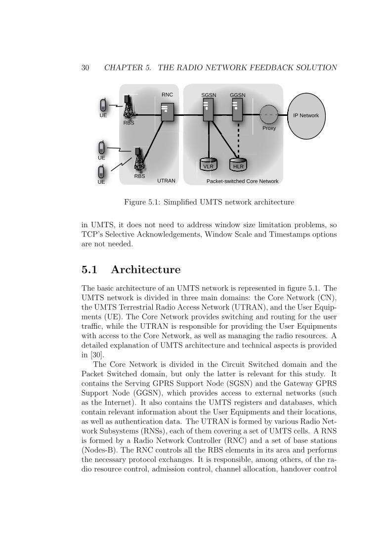
5.1 Architecture
The basic architecture of an UMTS network is represented in figure 5.1. TheUMTS network is divided in three main domains: the Core Network (CN),the UMTS Terrestrial Radio Access Network (UTRAN), and the User Equip-ments (UE). The Core Network provides switching and routing for the usertraffic, while the UTRAN is responsible for providing the User Equipmentswith access to the Core Network, as well as managing the radio resources. Adetailed explanation of UMTS architecture and technical aspects is providedin [30].
The Core Network is divided in the Circuit Switched domain and thePacket Switched domain, but only the latter is relevant for this study. Itcontains the Serving GPRS Support Node (SGSN) and the Gateway GPRSSupport Node (GGSN), which provides access to external networks (suchas the Internet). It also contains the UMTS registers and databases, whichcontain relevant information about the User Equipments and their locations,as well as authentication data. The UTRAN is formed by various Radio Net-work Subsystems (RNSs), each of them covering a set of UMTS cells. A RNSis formed by a Radio Network Controller (RNC) and a set of base stations(Nodes-B). The RNC controls all the RBS elements in its area and performsthe necessary protocol exchanges. It is responsible, among others, of the ra-dio resource control, admission control, channel allocation, handover control

5.1. ARCHITECTURE 31
Proxy Server
terminal-proxy TCP connection server-proxy TCP connection
variable BW / delay
Figure 5.2: Radio Network Feedback scenario
and broadcast signalling. A RBS covers one or more cells, and communicatesdirectly with the User Equipments that are located in the served area. It isresponsible for transmission and reception over the air interface, as well asmodulation and demodulation, WCDMA channel coding, error handling andclosed loop power control.
Figure 5.2 shows the main elements that are relevant from the RadioNetwork Feedback point of view. Some 3G network elements (such as theSGSN and GGSN), as well as their interconnections, are omitted on theassumption that the 3G core network is properly dimensioned and that themain bottleneck is the wireless link. Thus, only the elements that play animportant role on the TCP connection and adaptation are represented:
• All the connections are initiated by the mobile terminals, which at-tempt to send requests to the remote servers.
• The RNC plays a major role in the adaptation mechanism, as it hasimportant information about the available bandwidth assigned to ev-ery user. This information is sent to the proxy, both periodically andupon every bandwidth change, in order to update the connections TCPparameters. It also forwards all the packets sent from and towards theterminals.
• The proxy, which is located between the UMTS core network elementsand the external network, forwards the requests from the terminals, andadapts the TCP parameters of the connections in order to optimize thedata transfer.
• Remote servers receive requests from the proxy (on behalf of theterminals) and send the requested files back.
For the sake of simplicity, the RBS can be skipped from the scenario.Its forwarding and retransmission mechanisms can be modeled as variable

32 CHAPTER 5. THE RADIO NETWORK FEEDBACK SOLUTION
bandwidth and delay. The result is that all the links (except the terminal-RNC link) are high-bandwidth, low-delay links, while the terminal-RNC linksuffers from high delay as well as bandwidth and delay variations.
5.2 Scenario
In a typical scenario, a mobile terminal attempts to establish a connection toone of the remote servers. The initial TCP connection establishment packet(SYN) is received by the proxy, which returns the corresponding reply (SYN-ACK), and the terminal-proxy connection is completed. It also establishes aconnection to the specified server, and forwards the initial file request sent bythe client. The result is that two different TCP connections are established(one between the terminal and the proxy, and the other one between theproxy and the remote server), being the proxy responsible for forwarding thepackets between both of them. Note that the proxy is not transparent, asthe terminal explicitly establishes a TCP connection with it, similar to thebehavior of a typical HTTP proxy.
Upon receipt of the request, a remote server begins to send the file follow-ing the traditional TCP algorithms, including Flow and Congestion Control.All the transferred data is received by the proxy, where it is buffered in orderto be sent to the mobile terminal as soon as possible. Note that, while theremote server modifies its TCP parameters according to its own TCP imple-mentation, the proxy receives every packet at the highest rate possible andbuffers it. Then, it can use whatever TCP parameters it needs in order toadapt the connection to the variable wireless conditions. This way, the TCPconnection to the remote server does not suffer the effects of the wirelesslink, and the connection to the mobile terminal is tailored to the current linkcharacteristics. At the same time, it is totally transparent to both endpoints,and the only problem is the need for having a per-flow dedicated buffer andconnection state at the proxy.
The adaptation algorithm in the proxy is based on the information re-ceived from the RNC, whose aim is to help the proxy draw an accuratepicture of the current wireless link characteristics. Most TCP versions tryto estimate the available bandwidth by means of RTT measurement andloss events, or, like TCP Vegas [31], by computing an estimate of the queuelength at the bottleneck. However, in the case of UMTS, such informationis already known by the RNC, and it can be forwarded to the proxy. Hence,there is no need to implement a complex algorithm to infer an estimation outof (possibly inaccurate) measurements. The 3G network elements can coop-erate with the proxy to achieve a high utilization of the available resources.
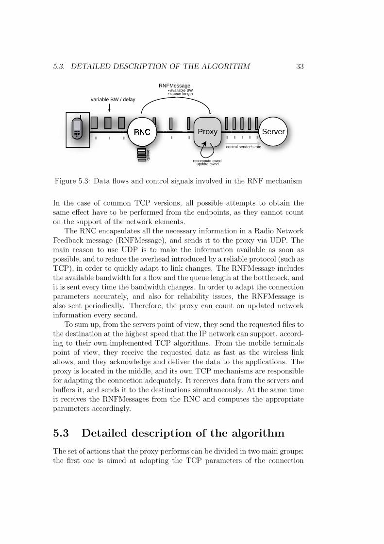
5.3. DETAILED DESCRIPTION OF THE ALGORITHM 33
Proxy Server
variable BW / delay
RNFMessageavailable BWqueue length
control sender's rate
recompute cwndupdate cwnd
queu
e
Figure 5.3: Data flows and control signals involved in the RNF mechanism
In the case of common TCP versions, all possible attempts to obtain thesame effect have to be performed from the endpoints, as they cannot counton the support of the network elements.
The RNC encapsulates all the necessary information in a Radio NetworkFeedback message (RNFMessage), and sends it to the proxy via UDP. Themain reason to use UDP is to make the information available as soon aspossible, and to reduce the overhead introduced by a reliable protocol (such asTCP), in order to quickly adapt to link changes. The RNFMessage includesthe available bandwidth for a flow and the queue length at the bottleneck, andit is sent every time the bandwidth changes. In order to adapt the connectionparameters accurately, and also for reliability issues, the RNFMessage isalso sent periodically. Therefore, the proxy can count on updated networkinformation every second.
To sum up, from the servers point of view, they send the requested files tothe destination at the highest speed that the IP network can support, accord-ing to their own implemented TCP algorithms. From the mobile terminalspoint of view, they receive the requested data as fast as the wireless linkallows, and they acknowledge and deliver the data to the applications. Theproxy is located in the middle, and its own TCP mechanisms are responsiblefor adapting the connection adequately. It receives data from the servers andbuffers it, and sends it to the destinations simultaneously. At the same timeit receives the RNFMessages from the RNC and computes the appropriateparameters accordingly.
5.3 Detailed description of the algorithm
The set of actions that the proxy performs can be divided in two main groups:the first one is aimed at adapting the TCP parameters of the connection

34 CHAPTER 5. THE RADIO NETWORK FEEDBACK SOLUTION
between the proxy and the mobile terminals (Proxy-Terminal control), whilethe second one is focused on the TCP connection between the proxy and theremote servers (Proxy-Server control).
5.3.1 Proxy-Terminal control
The objective of the Proxy-Terminal control is to tailor the TCP connectionto the wireless link characteristics, and to adapt its parameters to the varyingnetwork conditions. It is based on the Radio Network Feedback informationreceived from the RNC, included in the RNFMessages, and it addresses mostof the problems of the wireless link.
Variables and parameters
In order to adapt the connection to the wireless link characteristics, theproxy updates and modifies a set of variables and parameters. These eitherrepresent the link state or determine the TCP sending rate, and they can bedivided into input signals and output signals.
bτ
input signals qref
qRNC
recvwndwnd
output signals cwndBDP
Table 5.1: Input and output signals for the Terminal-Proxy control
The proxy makes use of the following input signals:
Available bandwidth In order to perform all the computations based onupdated information, the proxy uses a variable called b, which repre-sents the available bandwidth for a determined TCP flow. This vari-able is updated whenever the proxy receives a RNFMessage, and itcontributes to the estimation of the instantaneous size of the pipe.
Estimated path delay The current delay of the path from the proxy to theterminal is not provided by the RNC. The basic TCP versions include amechanism to compute the Round-Trip Time, but many received acksneed to be sampled in order to obtain a reasonably accurate estimation,

5.3. DETAILED DESCRIPTION OF THE ALGORITHM 35
so an adequate value is only available after some RTTs. Instead, theproxy uses a predefined value that represents an average delay of thepath, τ , which does not include queueing delays. It performs allthe computations with this value, and corrects the resulting parametersaccording to other link measurements.
Desired queue length One of the main objectives of the proxy is to main-tain a controlled queue length at the RNC, in order to prevent bufferunder and overflows. The size of this queue depends on the maximumtransmission rate, and the magnitude of the delay changes. It is aconstant value (qref ) that the proxy will try to maintain, based on thefeedback information received from the RNC.
Actual queue length The actual value of the RNC queue length, qRNC , isincluded in the periodic RNFMessages sent by the RNC to the proxy.This value is compared to the desired queue length, qref , in order toperform the necessary corrections.
Terminal’s receive window TCP’s receive window, recvwnd, reflects theamount of free buffer space at the receiver. It is used by the senderto compute the sending window wnd, thus it reduces the sending rateif the receiver is running out of space. In this report, it is assumedthat the mobile terminal can always handle all the data that the proxysends, so the terminal’s recvwnd never places a limit on the value ofwnd. This way, the sending rate towards a terminal is completelydetermined by the proxy’s congestion window value.
These input signals are used to obtain the following control signals:
Sending window TCP’s sending window, wnd, limits the amount of unac-knowledged data that the sender (in this case the proxy) can handle.It determines how much data can be sent per round-trip time, thus it isdirectly related to the transmission rate. It is the main variable neededin order to control the behavior of the TCP sender, and depends onthe values of the congestion window cwnd and the receiver’s receivewindow, recvwnd.
Congestion window TCP’s congestion window (cwnd) is computed by theTCP sender, and it contributes to the value of the sending window. Itis the result of applying all the congestion control algorithms. Its valueand its growing rate greatly affect the efficiency of the TCP sender.
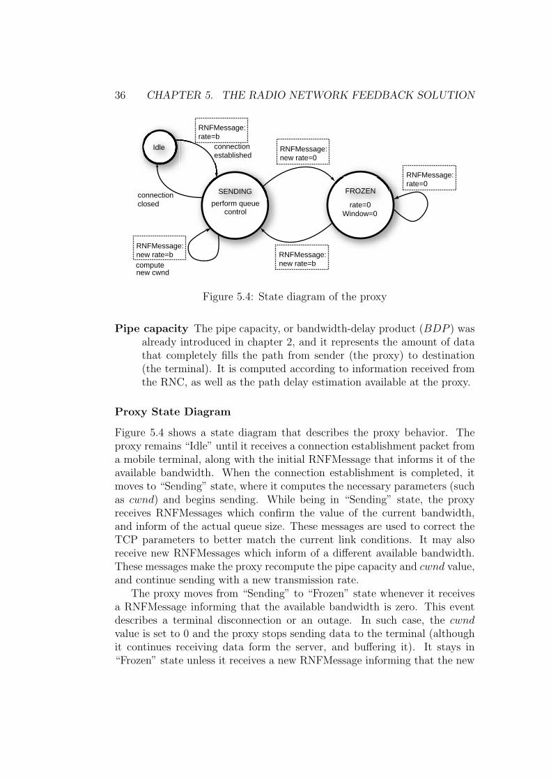
36 CHAPTER 5. THE RADIO NETWORK FEEDBACK SOLUTION
Idle
SENDING FROZEN
perform queue rate=0Window=0
RNFMessage:rate=0
RNFMessage:new rate=0
RNFMessage:new rate=b
RNFMessage:new rate=b
connectionestablished
connectionclosed
RNFMessage:rate=b
control
new cwndcompute
Figure 5.4: State diagram of the proxy
Pipe capacity The pipe capacity, or bandwidth-delay product (BDP ) wasalready introduced in chapter 2, and it represents the amount of datathat completely fills the path from sender (the proxy) to destination(the terminal). It is computed according to information received fromthe RNC, as well as the path delay estimation available at the proxy.
Proxy State Diagram
Figure 5.4 shows a state diagram that describes the proxy behavior. Theproxy remains “Idle” until it receives a connection establishment packet froma mobile terminal, along with the initial RNFMessage that informs it of theavailable bandwidth. When the connection establishment is completed, itmoves to “Sending” state, where it computes the necessary parameters (suchas cwnd) and begins sending. While being in “Sending” state, the proxyreceives RNFMessages which confirm the value of the current bandwidth,and inform of the actual queue size. These messages are used to correct theTCP parameters to better match the current link conditions. It may alsoreceive new RNFMessages which inform of a different available bandwidth.These messages make the proxy recompute the pipe capacity and cwnd value,and continue sending with a new transmission rate.
The proxy moves from “Sending” to “Frozen” state whenever it receivesa RNFMessage informing that the available bandwidth is zero. This eventdescribes a terminal disconnection or an outage. In such case, the cwndvalue is set to 0 and the proxy stops sending data to the terminal (althoughit continues receiving data form the server, and buffering it). It stays in“Frozen” state unless it receives a new RNFMessage informing that the new

5.3. DETAILED DESCRIPTION OF THE ALGORITHM 37
available bandwidth is different to zero. Then, the proxy computes the newpipe capacity, sets cwnd accordingly and resumes the transmission.
Control algorithm
The control algorithm for the connection between the proxy and a terminalcan be divided in two main parts.
The first one is event-driven, and takes place whenever the proxy is in-formed of a change in the bandwidth. It consists on computing an initialcongestion window, that depends on the available bandwidth and the pathdelay estimation.
The second one takes place periodically, every second after a bandwidthchange. It consists in monitoring the queue length, based on the informationsent by the RNC, and adjusting the congestion window value computed inthe first part. The idea is to compensate for possible inaccuracies in theprevious computation, as well as for possible delay changes in the path tothe destination.
This way, whenever the proxy is informed of a change in the bandwidthof the path, the following actions are performed:
• First, the pipe capacity is computed as a product of the available band-width and the predefined estimation of the delay of the path. This pipesize describes the maximum amount of data (or packets, after the ap-propriate conversion) that the pipe can absorb without building a queuein any of the intermediate buffers:
BDP = τ · b (5.1)
• Then, the proxy sets its cwnd to this value, plus some extra packets tocreate a small queue of a determined size at the bottleneck (the RNC).The idea is that the wireless channel is an expensive and scarce resource,so it must always be fully utilized. The purpose of the small queue atthe bottleneck is to reduce the impact of possible delay fluctuations, andto ensure that there is always at least one packet to transmit throughthe wireless link:
cwnd = BDP + qref (5.2)
• While setting cwnd to its final value ensures a high link utilization andminimum delay, it can significantly increase the queue size at the bot-tleneck. This effect is important during Slow Start and after anoutage, and must be dealt with. Although the proxy is using a cwnd

38 CHAPTER 5. THE RADIO NETWORK FEEDBACK SOLUTION
value that suits the pipe capacity, increasing the window size and send-ing cwnd packets at the highest rate creates a burst that the bottlenecklink cannot absorb, so most packets will be queued at the RNC. Thisproblem can be solved if the proxy introduces a small delay betweenthose cwnd packets, instead of sending them as fast as the link allows.This burst-smoothing technique is based on periodic interruptions thatdetermine when a packet should be sent, and it was initially introducedin [17] to reduce the impact of bursts in Slow Start. The result is thatcwnd packets are sent, but they are evenly distributed in a whole RTT,so their impact on the RNC buffer is reduced.
• Finally, the sending window is computed as in equation 5.3. Note thatwe have assumed that recvwnd never places a lower limit on the valueof wnd, therefore:
wnd = min{recvwnd, cwnd} = cwnd (5.3)
For every received RNFMessage received after a bandwidth change, andif the bandwidth is the same as the previous RNFMessage, the value of cwndis adjusted the following way:
• First, actual value of the RNC queue is compared to the desired queuelength, and the difference is obtained:
�q = qref − qRNC (5.4)
• If the absolute value of this difference is less or equal to one, it isignored. The reason for this is that during the simulations it was ob-served that the instantaneous length of the queue can oscillate slightlyaround the average length. Oscillations of 1 packet are natural andare a result of TCP dynamics (and they do not necessarily represent avariation in the RTT of the path), therefore the proxy should not reactto such variations:
�q =
{ �q if |�q| > 10 otherwise
(5.5)
• Finally, this difference is added to the previous value of the congestionwindow. This means that the cwnd is increased or decreased in orderto compensate for possible variations in the RNC queue length:
cwnd(n + 1) = cwnd(n) + �q (5.6)
To sum up, figure 5.5 illustrates the set of actions and decisions that theproxy performs upon the receipt of a RNFMessage. This includes identifyinga bandwidth change, as well as the queue control algorithm.

5.3. DETAILED DESCRIPTION OF THE ALGORITHM 39
( (
YES
NO
YES
NO
YES
NO
RNFMessage received
received BW
current BW ?
recompute cwndaccording to new BW
received queue
desired queue ?
received queuedesired queue <1 ?
cwnd=cwnd- received queuedesired queue
Figure 5.5: Flow diagram of the queue control algorithm
Addressed problems
Slow Start latency One of the problems that the proxy needs to addressis the significant increase in the total transfer time introduced by the SlowStart phase, as it was explained in Section 2.1.
However, and unlike in the case of TCP, in the RNF scenario the proxyreceives a RNFMessage as soon as the connection begins, informing it of theavailable bandwidth for the connection. Thus, there is no need to use a smallsending rate to probe the bandwidth, as it is not an unknown value any more.The proxy can begin the transmission at the maximum rate that the wirelesslink can support, as explained in section 5.3.1.
Figure 5.6 illustrates the improvement brougth by the queue smoothingalgorithm. In it, the proxy sends a determined number of packets at thehighest rate offered by its high-bandwidth link, so they arrive in a burst atthe RNC, where they are queued. The opposite case is represented in Figure5.7, where the proxy purposely increases the separation between packets, inorder to reduce the peak queue size at the bottleneck.
Bandwidth variation In principle, the whole bandwidth assigned to theHSDPA channel in a UMTS cell is equally shared among all the users locatedin that cell. Therefore, bandwidth variations are inherent, as an increase in

40 CHAPTER 5. THE RADIO NETWORK FEEDBACK SOLUTION
Proxy
medium BW - high delay high BW - low delay
queue
Figure 5.6: Impact of bursts on queue size
Proxy
medium BW - high delay high BW - low delay
queue burst smoothing
Figure 5.7: Queue reduction through burst smoothing
the number of users leads to a decrease in the amount of bandwidth assignedto each of them, and vice-versa. In practice, HSDPA is expected to provideup to 2Mbps, so variations up to 1Mbps could be possible.
As explained before, TCP is unable to quickly adapt to bandwidth vari-ations. In order to avoid this problem, there is a need to find a mechanismto quickly adapt the size of cwnd to the instantaneous pipe size.
Proxy
BW = R (Kbits/s)
Figure 5.8: Steady state of the connection before bandwidth variation
As it has been described before, the proxy periodically receives a RNFMes-sage from the RNC, informing of the current available bandwidth. As soonas the message is received, the proxy can easily compute the current size of

5.3. DETAILED DESCRIPTION OF THE ALGORITHM 41
Proxya)
BW = 2*R (Kbits/s)
b)
BW = 2*R (Kbits/s)
Figure 5.9: Adaptation of the cwnd to bandwidth variation
the pipe and adapt its cwnd to the new link characteristics, i.e., it can imme-diately increase or decrease the window to match the new bandwidth. Thisway, the proxy can always use a suitable window size, and properly react inthe face of bandwidth changes.
Figure 5.8 shows a situation where the proxy is using a cwnd value thatsuits the available bandwidth, in order to maintain a constant queue lengthof 4 packets. Figure 5.9 compares the results after the bandwidth is doubled.In case a), the proxy does not immediately adapt its cwnd to the new pipecapacity. Therefore the queue is drained, and it is not able to keep up with thenew rate, leading to bandwidth under-utilization. Case b) shows a situationwhere the proxy, after being informed of the new bandwidth, increases thecwnd value. This way, its transmission rate is increased in order to matchthe new bandwidth conditions, and the RNC-terminal link is fully utilized.
Disconnections and outage Disconnections (introduced in section 2.1)are one of the worst problems that TCP has to face in mobile scenarios. Theycan introduce huge delays and significantly decrease the link utilization. Forthat reason, they are one of the main issues that the RNF mechanism triesto deal with.
The proxy should stop sending packets in presence of a disconnection,and immediately resume the transmission when the link recovers. To achievethis, it is necessary to make the proxy realize that the destination is reach-able again after a disconnection. Some approaches like [18] and [19] try toaccomplish this by having the mobile terminal inform the TCP sender of areconnection. However, it is desirable to perform the adaptation without the

42 CHAPTER 5. THE RADIO NETWORK FEEDBACK SOLUTION
need to involve the destinations. Moreover, it is not a good idea in a 3Gscenario to depend on the terminals in order to properly utilize the UMTSnetwork resources.
The RNF mechanism overcomes this problem by taking advantage of theinformation provided by the UMTS network itself. As explained in section5.3.1, the proxy bases its behavior on the bandwidth information sent bythe RNC. A basic TCP sender detects an outage or a terminal disconnec-tion when it stops receiving acks from the destination, which causes manytimeouts. Thus, it takes the sender at least one RTT to realize that thedestination is not reachable any more. On the contrary, the RNC sends aRNFMessage to the proxy as soon as the bandwidth changes. Therefore, itwill immediately send a message informing that the available bandwidth iszero in the face of a disconnection.
As soon as the proxy receives a RNFMessage that informs of a nullbandwidth, it understands that the destination is unreachable, and entersFROZEN state (as described in Figure 5.4). While being in this state, theproxy “freezes” the connection, i.e., it closes cwnd, stops sending packets, andignores any subsequent timeouts or received acks. It continues receiving pe-riodic RNFMessages, but it only checks the advertised available bandwidth,waiting for a non-zero value.
According to [1], during a disconnection a basic TCP sender would enterExponential Backoff, where it would send exponentially separated probes inorder to detect a reconnection. This behavior is needed in basic TCP imple-mentations, because in principle, a TCP sender does not have any other wayto detect that the destination is reachable again. However, it is unnecessaryin the RNF scenario, as the reconnection will be explicitly indicated by theRNC. There is no reason for the proxy to probe the path, because as long asit does not receive a RNFMessage with this information, it can assume thatthe destination is not reachable yet.
The proxy stays in FROZEN state until it receives a RNFMessage thatincludes a bandwidth other than zero, which informs of the destination’s re-connection. Then, it uses the newly received bandwidth and its path delayestimation to recompute the pipe capacity. It sets the value of cwnd to thepipe size plus some extra packets, moves to SENDING state, and resumes thetransmission. This behavior reduces the idle period after a reconnection in-troduced by Exponential Backoff, as shown in figure 5.10. Moreover, it skipsthe Slow Start phase after the reconnection, increasing the link utilizationeven more.
However, increasing the cwnd value from zero to the final value can leadto burst problems, as described in section 5.3.1. For that reason, the proxyimplements the same mechanism to smooth the initial burst that was intro-
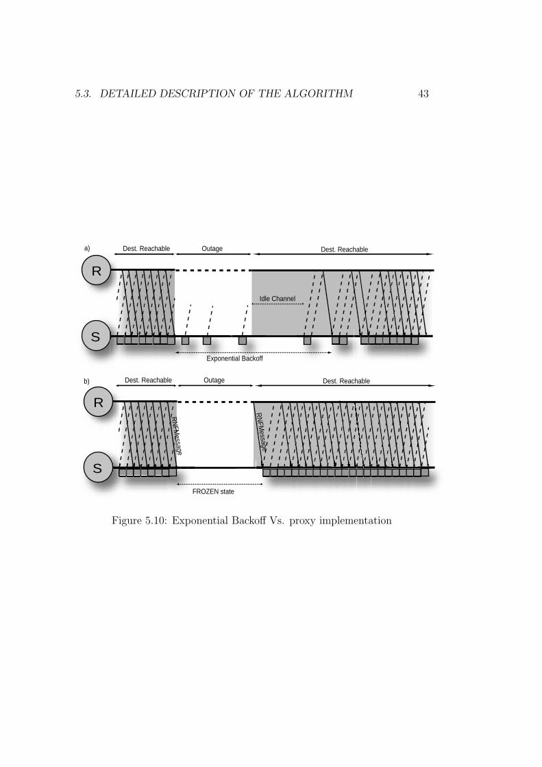
5.3. DETAILED DESCRIPTION OF THE ALGORITHM 43
R
S
Exponential Backoff
OutageDest. Reachable Dest. Reachable
Idle Channel
R
S
OutageDest. Reachable Dest. Reachable
FROZEN state
RN
FMessage
RN
FMessage
a)
b)
Figure 5.10: Exponential Backoff Vs. proxy implementation

44 CHAPTER 5. THE RADIO NETWORK FEEDBACK SOLUTION
duced above. The result is that the bandwidth utilization is the same asit would be if cwnd packets were sent at once, but the queue size is muchsmaller.
Limited buffer at the RNC and delay variation In a UMTS scenario,where the Core Network is assumed to be well dimensioned, the path betweenthe RNC and the terminal has the lowest bandwidth, thus it becomes thebottleneck.
As explained above, all the packets that the sender injects into the net-work and that cannot be absorbed (i.e., the difference between the sender’swnd and the pipe capacity) have to be queued somewhere in the path betweensender and destination. Excess packets will be queued at the bottleneck, i.e.,the RNC buffers. The RNC is supposed to have enough processing speed,therefore the main reason for packet queuing is that the outgoing links areslower than the incoming one. The RNC keeps a per-destination buffer, sopackets from different connections, in principle, do not affect other connec-tions’ performance.
The resulting effect is that, for every connection, a queue will build upat the RNC. In principle, the size of this queue is the difference between thenumber of packets being sent per RTT and the number of packets that thepipe can absorb. However, varying network conditions (such as bandwidthor delay) and TCP dynamics cause the queue length to oscillate.
As explained in section 5.3.1, the proxy tries to maintain a fixed queuelength at the RNC. The reason for this decision is to ensure that there isalways a packet to send through the wireless link. In general, the queueneeds to be long enough to avoid buffer underflow (i.e., a situation when thewireless link is willing to accept more data, but there is no data to send).On the other hand, it has to be short enough in order to reduce the queuingdelay, as well as save memory and avoid scalability problems. In summary,the size of the queue is a tradeoff between buffer space and wireless linkutilization. A huge queue ensures that there will be a packet to send in anycase, but it increases the buffer needs as well as queuing delay.
If the average path delay that the proxy uses for its computations werean accurate representation of the real delay, and if TCP’s behavior weredeterministic, the size of the RNC queue would always be:
qRNC = cwnd − BDP
However, it is unlikely that in a UMTS scenario (where mobility is aninherent characteristic of the terminals) the wireless link delay will remain

5.3. DETAILED DESCRIPTION OF THE ALGORITHM 45
constant. The result is that the proxy’s average path delay will probablydiffer from the real delay.
Assuming that the proxy has computed a pipe capacity of BDP packets,and is has a desired que length of qref packets, its cwnd size should be BDP +qref . But let’s assume that the delay of the path is halved. The proxy cannotpossibly notice it, as it doesn’t count on RTT measurements to compute thepipe capacity. Then, the new pipe size will be BDP/2, so the cwnd valueshould now be BDP/2+qref . However, the proxy keeps on using BDP +qref ,based on its inaccurate computation of the pipe capacity. The result is thatthe queue at the RNC will grow in BDP/2 packets. The opposite wouldoccur if the delay of the wireless link increased, leading to possible bufferunderflow. Having an arbitrary queue length is highly undesirable, and itcan lead to scalability problems as well as link under-utilization. There is aneed for a mechanism in order maintain the desired queue length qref , evenin the face of delay variation and inaccurate cwnd computations.
The working point of the proxy (the value of qref ) must ensure that theRNC buffer will not be completely drained when the path RTT increases.Therefore, it seems reasonable to keep a queue slightly longer than the worstqueue variation possible. Delay variations affect the RNC queue length ac-cording to
�qdelay = �τ · bThen, the qref value should fulfill the following condition:
qref ≥ �τmax · bmax
Having a fixed qref value can always lead to too big or too small buffersizes. If qref is chosen to deal with the biggest changes possible, as above, itis possible to ensure that there will not be any buffer underflows. However,most of the times qref will be higher than necessary. Ideally, qref should betailored to the current conditions, such as the current bandwidth instead ofthe maximum one. This issue is left for further study.
As explained in section 5.3.1, the algorithm tries to correct any possibledeviations from the expected queue length, by monitoring the actual lengthvalue and comparing it to a reference. This process continues until the band-width changes, what causes the RNC send an instant RNFMessage with thenew bandwidth, and makes the proxy recompute all the parameters again.
Note that this behavior is very similar to that of TCP Vegas. The maindifference is that, while TCP Vegas makes an estimation of the queue lengthat the bottleneck, the proxy receives the actual queue value from the RNC.In both cases, the response to queue variation is similar, and it consists in

46 CHAPTER 5. THE RADIO NETWORK FEEDBACK SOLUTION
increasing or decreasing the congestion window value in order to compensatethe variations. [32] shows that this behavior ensures that the queue sizeconverges to a value, by applying a fluid model.
5.3.2 Proxy-Server control
One of the main problems of splitting the server-destination connection intwo is the need to buffer and forward the packets towards the terminals. Theproxy receives data packets from the servers at the highest speed possibleand buffers them, while it tries to send them to the mobile terminals simul-taneously. However, the sending rate towards the terminals is, in general,much lower that the rate at which it receives data from the servers. Evenworse, the proxy is not able to send anything to the destinations during adisconnection, but it keeps on receiving packets. Therefore, the amount ofbuffered data can increase considerably, leading to scalability problems.
An straightforward solution to this problem is to set a limit on the amountof data per connection that the proxy can buffer. The idea behind thisapproach is that it is more convenient to keep the data in the remote servers,rather than in the proxy. The former should dedicate memory to buffera determined amount of data, but never more than a fixed limit. Thus, aremote server should be slowed down when the proxy is running out of space.
Fortunately, TCP provides the means to implement this behavior. Itincludes Flow Control mechanisms in order to deal with situations wherethe receiver cannot cope with all the data sent by the sender. As describedin section 1.1.1, the receiver’s recvwnd is sent back in every ack in orderto prevent the sender from overflowing the destination’s buffers. This way,recvwnd represents the amount of free space at the receiver, and it sets alimit on the sender’s window wnd. Then, it can be easily used to slow downor speed up the sender when necessary.
The objective of the Proxy-Server control is to influence the behaviorof the remote server, without the need to change the TCP version that itimplements. It is aimed at slowing down or speeding up the sender, accordingto the available buffer space at the proxy. The objective is to keep the amountof buffered data within a limit, in order to provide scalability.
Variables and parameters
The proxy uses two input signals that reflect the amount of free buffer spaceat the proxy, and one output signal that is used to control the server’s sendingrate.

5.3. DETAILED DESCRIPTION OF THE ALGORITHM 47
input signals Btot
Boutput signals recevwnd
Table 5.2: Input and output signals for the Server-Proxy control
Available buffer space For every connection, and depending on its char-acteristics, the proxy dedicates a determined amount of buffer space,Btot. It is stated in [11] that the bandwidth-delay product is a reason-able measure of the amount of buffer space that a TCP flow should begranted.
Current buffered data The proxy keeps a variable (B) that representsthe amount of data that the proxy has received, but has not sent yet(i.e., the amount of data that it has buffered). This value is updatedwhenever a new packet is received from the remote server.
Proxy’s receive window The value of the proxy’s recevwnd represents theamount of free buffer space at the proxy, and it can be used to adaptthe behavior of the remote server. As it was shown in Section 1.1.1, thesending window is computed as the minimum of recvwnd and cwnd.Thus, is is possible to slow down the sender’s transmission rate byreturning a small enough recvwnd with every ack.
Control algorithm
The proxy-server control algorithm uses the recvwnd value that is returnedin every ack to the sender, in order to influence its sending rate. The proxyperforms the following actions during a connection to a server:
• First, the proxy computes the amount of buffer space that it will ded-icate for the connection:
Btot = τ · b (5.7)
• Every time a packet is sent to the terminal, or a packet is receivedfrom the remote server, the amount of buffered data is updated, andthe amount of free buffer space is computed. Finally, the value of theproxy’s recvwnd is set to this difference, thus it represents the amountof free buffer space at the proxy:
recvwnd = Btot − B (5.8)

48 CHAPTER 5. THE RADIO NETWORK FEEDBACK SOLUTION
• The remote server will receive this value in the returning acks and itwill use it to compute its own sending window, as in 5.3. In this case,however, the recvwnd may limit the value of wnd:
wnd = min{recvwnd, cwnd} (5.9)
Addressed problems
Limited buffer size at the proxy The resulting effect of the proxy-servercontrol algorithm is that the server’s sending window is increased when morebuffer space at the proxy is available, and it is reduced when free buffer spaceat the proxy decreases. In the last case, it receives data at a lower rate, whichprevents buffer overflowing and reduces the amount of memory required.
A problem might arise if the buffer for a determined flow is full. Then, theproxy would return a recvwnd of zero, what would cause the server to stopthe transmission until it receives an ack with a non-zero recvwnd. However,if the server is not sending data to the proxy, there is no way for the formerto send an ack to update the recvwnd value. TCP [1] provides a mechanismto deal with such situation, which consists in forcing the sender into persistmode when it receives the zero window update. While being in persist mode,the sender does not close its congestion window, neither does it suffer fromretransmit timeouts. Instead, it sends periodic probes, called “Zero WindowProbes” (ZWPs), until the receiver’s window opens up again.
However, this behavior can introduce an extra delay, if the buffer isdrained during the interval between two ZWPs. In such case, the proxycould run out of buffered data, but the remote server would believe that thebuffer is still full, and it would remain in persist mode until the next ZWPwere sent. A solution to this problem was initially introduced in [18], andlater refined in [19]. It consists on having the receiver send a duplicated ackas soon as its recvwnd opens, instead of waiting for a ZWP from the sender.This way, the sender receives an instant window update, and it can resumethe transmission immediately. This approach is taken by the proxy, in orderto prevent servers from sending too much data, as well as eliminating thewaiting time between two ZWPs.
5.4 Proxy control model
5.4.1 Overview of the queue control algorithm
As explained in section 5.3.1, the main objective of the queue control al-gorithm is to maintain a fixed per-flow queue length at the bottleneck (the

5.4. PROXY CONTROL MODEL 49
q
Proxy +ref
db
qRNC
link
proxyq
Figure 5.11: Block diagram of the proxy algorithm.
RNC), by updating its congestion window to compensate for possible varia-tions in the pipe round-trip time.
Using the cwnd computed upon a bandwidth change at the proxy is notenough to keep a constant queue length at the RNC. This is mainly dueto variations in the link delay that are translated into variations of the pipecapacity, as it is usual in wireless links. Whenever the link delay changes, thepreviously computed BDP no longer represents the pipe capacity, thus thequeue length at the RNC will change. To compensate for these variations,the proxy monitors periodically the length of the RNC queue (qRNC) andmodifies its congestion window accordingly, until it is informed of a newchange in the transmission rate that will cause the recalculation of the pipesize again.
The whole process (including the queue monitoring and window updat-ing) takes place between the proxy and the RNC, and can be represented asa closed loop system described by the block diagram in figure 5.11. The dia-gram describes a system that tries to adapt its output qRNC , that representsthe actual queue length at the RNC, to a reference signal qref (the desiredqueue length). It does so by adjusting the congestion window value cwndto compensate for the variable link delay, which can be modeled as a distur-bance function dlink that modifies the output. The feedback loop representsthe queue sampling and monitoring, while the P block models the algorithmused by the proxy to adjust the window value.
Note that there is a direct relation between the actual congestion windowused by the proxy and the length of the queue. In absence of delay variations,the queue length is the difference of the current congestion window cwnd andthe pipe capacity, i.e all the packets that the pipe is not able to absorb arequeued at the bottleneck.
On the other hand, a variation in the delay is translated into the pipe

50 CHAPTER 5. THE RADIO NETWORK FEEDBACK SOLUTION
absorbing more or less packets, therefore decreasing or increasing the queuelength. This delay variation is described by the disturbance dlink that addsor withdraws packets from the queue,
dlink = (τ − τ) · b (5.10)
where τ is the proxy’s predefined estimation of the path delay, and τ isthe actual delay of the path.
Therefore, the resulting queue at the RNC consists of a contribution ofthe proxy (qproxy), and a contribution of the possible variation in the linkdelay (dlink):
qRNC = qproxy + dlink (5.11)
The latter is described, as explained before, by equation 5.10. The formeris the difference between the current cwnd that the proxy is using, and thecomputation of the pipe capacity performed at the beginning of the phase:
qproxy = cwnd − BDP (5.12)
Note also that although the relation is linear (increasing the congestionwindow by p packets increases the queue by the same number of packets),it takes some time for the change to take effect (the queue needs a smallamount of time to build up). However, the interval between queue samplesis chosen to be longer that two times the value of RTT (1 second, while themaximum RTT from client to server is estimated in 400 ms), in order toallow queue stabilization. Hence, it can be safely assumed that the changein the cwnd value has already taken effect before the next iteration.
The following pseudo-code is executed in every iteration:
error = q_ref - q_RNC;
if (|error| is less or equal to one)
do nothing;
else
cwnd = cwnd + error;
This way, the new value of cwnd depends on the previous one, plus avalue that represents how different the RNC queue length from the desiredlength. Therefore, cwnd is updated in order to compensate for the possibledelay changes. Note that the cwnd is not updated if the magnitude of theerror (i.e., the �q defined before) is not bigger than one packet.

5.4. PROXY CONTROL MODEL 51
5.4.2 Analysis of the closed loop system
Although the model described in section 5.4.1 is an accurate representationof the proxy, further simplification can be performed to obtain a system thatis easier to analyze, and still has similar characteristics. While the initialcontroller prevents the system from reacting to small queue oscillations, it isa non-linear component that makes the system analysis much more complex.It can be skipped from the model without a significant modification of thesystem behavior. Hence it is assumed that the difference signal qref − qRNC
is suitable to control the algorithm without further processing. The onlydifference is that the proxy will correct variations of 1 packet on the queuelength, although the system can work without such corrections.
According to the pseudo-code description, and after the simplification isperformed, the system is described by the following equations in the discretetime domain:
qRNC(n + 1) = cwnd(n) + qref (n) − qRNC(n) − BDP (n) + dlink(n) (5.13)
cwnd(n + 1) = cwnd(n) + qref (n) − qRNC(n) (5.14)
To study the characteristics of the system, first the transfer function isobtained by transforming the equations above to the Z domain. By combiningthese equations, it is possible to obtain an expression of the output as afunction of the inputs:
QRNC(z) = Qref (z) − (1 − z−1) ·BDP (z) + z−1 · (1 − z−1) ·Dlink(z) (5.15)
This transfer function describes a system that is causal and stable.

52 CHAPTER 5. THE RADIO NETWORK FEEDBACK SOLUTION

Chapter 6
Simulations and results
In order to test the performance of the proxy setup, simulations were per-formed. Most of them aim to compare the proxy to the TCP protocol (TCPReno was chosen, as it is the most used version today), while others checkthe performance of the proxy in the absence of some of its features.
The simulations can be classified in two main groups, each of them withdifferent aims. One group is focused on comparing determined features ofthe proxy in the face of adverse conditions, such as long outages or abruptbandwidth changes. In some of these cases, the proxy performance is com-pared to that of TCP Reno, and the improvement is analyzed. The secondgroup is oriented to test the performance of both the proxy setup and a com-mon TCP sender, in some practical cases that could reflect a real situation.These cases are called Use Cases, and they are chosen to cover many of thepractical situations where TCP performance should be improved, such asweb browsing or FTP file downloading.
The simulations setup follows the scheme shown in figure 6.1, where twoseparated TCP connections are established, one between the terminal andthe proxy, and the other between the proxy and a remote server. The resultsare compared to those of the basic setup shown in figure 6.2, where thereis only one TCP connection from server to terminal, via the RNC. In thiscase, the communication is held through the basic TCP Reno agents providedwith the Network Simulator 2 (ns2) [33], as explained in section 6.1. In thatcase, the server is not informed of the wireless link, and no adaptation isperformed.
In figures 6.1 and 6.2, the links between the remote server, the proxy(if used) and the RNC are 2Mbps links. In general, the UMTS networkis assumed to be properly dimensioned to handle all the traffic, as well asthe link to the Internet. In such case, the limiting link will always be thewireless one, with lower (and variable) bandwidth. The link delays are set
53

54 CHAPTER 6. SIMULATIONS AND RESULTS
Proxy Server
terminal-proxy connection server-proxy connection
variable BW / delay
35.84 ms15.84 ms2 Mbps 2 Mbps
Figure 6.1: Scenario with proxy
Server
terminal-server TCP Reno connection
variable BW / delay
51.68 ms2 Mbps
Figure 6.2: Scenario without proxy
according to the figures, and the initial delay for the wireless link is 60 ms,although some variation may be added during some of the simulations. Theprocessing delay in the terminal is initially set to 40 ms, but the processingdelays in intermediate elements such as the RNC are not considered to besignificant. The TCP packet size is set to 1000 bytes, leading to 1040 bytesIP packets (and 40 bytes acks), while the transmission time in the wirelesslink, including link layer retransmissions, is described by:
Ttx =1460 · 8
b
These settings lead to an initial Round Trip Time (server-terminal-server)of 303 ms, although this figure will vary upon delay changes.
6.1 Tools and modules
The main tool used to perform the simulations was the Network Simulator2 (ns2), running over Cygwin on a PC Intel Pentium III processor.
In order to model the proxy behavior, as well as the intermediate elements,several C++ modules were added to the network simulator. A new TCP sinkwas developed in order to model a UMTS terminal with variable processing

6.2. GENERAL PERFORMANCE 55
delay. An application module was created for the remote servers, in order toanswer to requests with a configurable file size. This application was usedboth for FTP and HTTP modelling. The RNC behavior was completelymodelled in tcl language.
The proxy comprises an application which is in charge of forwarding pack-ets between the two TCP connections, as well as a TCP Reno Agent for theserver-proxy connection, and a RNFProxy Agent for the TCP connectiontowards the terminals. The application simply forwards packets in both di-rections, and controls the buffer size in order to slow down the remote server.The RNFProxy Agent is the modified TCP Agent in charge of adapting theparameters of the TCP connection between terminals and proxy, and includesmost of the proxy functionality.
6.2 General performance
6.2.1 Connection startup
In the first set of simulations, the main aspects that are tested are the perfor-mance on connection startup, the response to delay variation and the relia-bility of the UDP-based Radio Network Feedback, as well as the dependencyof both the proxy and TCP Reno behavior on the outage time.
The first simulation aims to compare the performance of the proxy tothe performance of TCP Reno, on connection startup. Figure 6.3 shows theresults for two different setups.
0 0.5 1 1.5 2 2.5 3 3.5 4 4.5 50
200
400
600
800
1000
1200
Time (s)
Rat
e (K
bits
/s)
ProxyInitWin=1InitWin=2InitWin=3Available BW
0 0.5 1 1.5 2 2.5 3 3.5 4 4.5 50
200
400
600
800
1000
1200
Time (s)
Rat
e (K
bits
/s)
Slow Start Threshold = 20 Slow Start Threshold = 50
ProxyInitWin=1InitWin=2InitWin=3Available BW
Figure 6.3: Comparison of startup performance with different initial win-dows, for Slow Start Threshold=20 and Slow Start Threshold=50
In both cases, a TCP connection is established in order to download a
56 CHAPTER 6. SIMULATIONS AND RESULTS
2MB file, and it is assigned an initial bandwidth of 1 Mbps, which should bebig enough to test the proxy behavior versus TCP’s Slow Start algorithm.In both graphs, the transmission rate is plotted as a function of time, forthe proxy setup (which adapts its initial window to the current BW), as wellas TCP Reno with an initial window of 1, 2 and 3 packets. The left plotrepresents a situation where TCP’s Slow Start threshold is set to 20 packets,so TCP connections enter an early Congestion Avoidance phase. In the rightplot, the Slow Start threshold is set to 50 packets.
Figure 6.3 shows a significant improvement of startup performance whenthe proxy is used, compared to TCP Reno (even with increased initial win-dows). The reason is that a TCP sender does not have information about theavailable bandwidth of the path, so it has to begin the transmission with thelowest rate possible. On the contrary, the proxy can set its initial value tofully utilize the bandwidth assigned to the connection, as its value is known.The improvement is even greater if TCP’s Slow Start Threshold is set to alow value (such as 20) in the Reno senders. The reason is that, in such case,the TCP sender enters an early Congestion Avoidance Phase, what reduceseven more the increase of the transmission rate.
6.2.2 Delay changes
A second simulation is intended to test the queue control algorithm of theproxy, in the face of link delay changes. How delay changes affect the queuedepends on the magnitude of the change as well as the link bandwidth, asgiven by
�qdelay = �τ · bwhere �qdelay represents the variation of the RNC queue length due to
delay changes, and �τ is the variation in the one-way delay between theRNC and the mobile terminal.
Delay variation is modelled through the use of cross-traffic. In a pathwith RTT � 300 ms, changes up to 100 ms in the Round Trip Time (50 msin both directions) could be possible. Figure 6.4 shows the response of theproxy in a situation where random delay changes (up to 33 ms) are appliedto the link, with a transmission rate of 1 Mbps. The plot shows the length ofthe queue at the RNC during some time, where delay changes are indicatedby vertical arrows. The horizontal line indicates the queue length that theproxy tries to maintain (5 packets for this simulation), while the shadowedarea within the dashed lines shows the margin where the proxy considersthat the queue length is close enough to the objective value (one packet upor down). Peaks in the queue length are caused by delay changes, while

6.2. GENERAL PERFORMANCE 57
the width of those peaks is determined by the reaction and response times(the time it takes the proxy to detect a change in the queue length and takeproper action).
10 15 20 25 30 35 40
1
2
3
4
5
6
7
8
9
Time (s)
Buf
fer
(pkt
s)
delaychange
delaychange
delaychange
delaychange
Figure 6.4: Performance of the RNC queue control algorithm in the face ofdelay changes, in terms of instantaneous value of the RNC queue length
The results show that the proxy successfully maintains an almost constantqueue length, as the length value always goes back to the desired range. Theamount of time during which the queue length is not controlled depends ondetection and reaction times. Detection time is limited by the fact that theinformation needs to be sent by the RNC to the proxy. The maximum time is1 second (in the worst case, assuming that the change takes place just aftera RNFMessage has been sent), plus the time it takes to receive the UDPpacket in the proxy (50 milliseconds). Reaction time depends on the time ittakes the proxy to modify the cwnd value (assuming the proxy has enoughprocessing power, it should be very small), plus the time the change needsin order to take effect (in the order of tens of milliseconds).
6.2.3 Algorithm reliability
The third simulation aims to test the reliability of the proxy control algorithmin the face of UDP packet losses. As explained before, UDP is not a reliableprotocol, and UDP packet loss or corruption in the link from the RNC to

58 CHAPTER 6. SIMULATIONS AND RESULTS
the proxy is possible. Therefore, retransmissions of RNFMessages have to bedealt with in some other way. For that reason, the RNC periodically sendsa new RNFMessage to the proxy, so if one message is lost the necessaryinformation will arrive within the next period. Figure 6.5 shows the resultsof the reliability test, where the setup is analogous to the previous case. Theleft plot shows a normal control of the queue length, while the right oneshows a situation where the RNFMessage right after the change is dropped,but the next one is received. Note that this is an especially unfavorable case,as the probability of losing or corrupting a packet is very small, and so is theprobability of losing the first packet that informs of a queue change.
10 15 20 25 30 35 40
1
2
3
4
5
6
7
8
9
Time (s)
Buf
fer
(pkt
s)
UDP
10 15 20 25 30 35 401
2
3
4
5
6
7
8
9
Time (s)
Buf
fer
(pkt
s)
UDP
Figure 6.5: Reliability of the control algorithm when a RNFMessage is lost
Figure 6.5 shows that sending the RNFMessages periodically is enoughto ensure that the algorithm keeps on working, even if one or more UDPpackets are lost or corrupted. The queue length is still controlled, even if theRNFMessage that informs of a change is lost, as shown in the graphs. Theeffect of one missing UDP packet is that the detection time increases, as theproxy will not receive updated information until the next RNFMessage issent. This effect is reflected on an increase on the time that the queue lengthis not within the desired bounds, but after the new detection and reactiontime it is controlled again.
On the other hand, figure 6.6 shows the effect of an abrupt delay change(100 ms increment in a 1 Mbps path)on the RNC queue length and trans-mission rate. The plots show the results both for a proxy performing queuecontrol, and a proxy where the queue control algorithm is not working. Theleft plot represents the length of the queue at the RNC in time, while theright one shows the time variation of the transmission rate. Both plots re-flect the improvement of the proxy queue control when the delay of the path
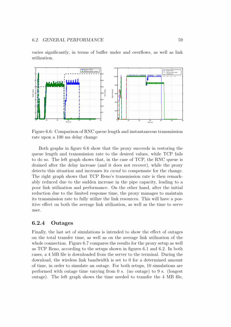
6.2. GENERAL PERFORMANCE 59
varies significantly, in terms of buffer under and overflows, as well as linkutilization.
0 10 20 30 40 50 600
1
2
3
4
5
6
7
8
Time (s)
Buf
fer
(pkt
s)
Queue controlWithout queue control
Delay (m
s)
50
100
150
200
250
300
350
0 10 20 30 40 50 600
200
400
600
800
1000
1200
Time (s)
Rat
e (K
bits
/s)
Queue controlWithout queue controlAvailable BW
Figure 6.6: Comparison of RNC queue length and instantaneous transmissionrate upon a 100 ms delay change
Both graphs in figure 6.6 show that the proxy succeeds in restoring thequeue length and transmission rate to the desired values, while TCP failsto do so. The left graph shows that, in the case of TCP, the RNC queue isdrained after the delay increase (and it does not recover), while the proxydetects this situation and increases its cwnd to compensate for the change.The right graph shows that TCP Reno’s transmission rate is then remark-ably reduced due to the sudden increase in the pipe capacity, leading to apoor link utilization and performance. On the other hand, after the initialreduction due to the limited response time, the proxy manages to maintainits transmission rate to fully utilize the link resources. This will have a pos-itive effect on both the average link utilization, as well as the time to serveuser.
6.2.4 Outages
Finally, the last set of simulations is intended to show the effect of outageson the total transfer time, as well as on the average link utilization of thewhole connection. Figure 6.7 compares the results for the proxy setup as wellas TCP Reno, according to the setups shown in figures 6.1 and 6.2. In bothcases, a 4 MB file is downloaded from the server to the terminal. During thedownload, the wireless link bandwidth is set to 0 for a determined amountof time, in order to simulate an outage. For both setups, 10 simulations areperformed with outage time varying from 0 s. (no outage) to 9 s. (longestoutage). The left graph shows the time needed to transfer the 4 MB file,

60 CHAPTER 6. SIMULATIONS AND RESULTS
depending on the outage time (on the horizontal axis), while the right graphshows the average link utilization, computed as
BWutil(%) =100
n·
n∑i=1
Ri
BWi
where Ri represents the transmission rate sampled in instant i, n is thenumber of samples and BWi is the instantaneous available bandwidth forthe connection.
0 1 2 3 4 5 6 7 8 90
10
20
30
40
50
60
70
80
90
100
110
Outage Time (s)
Utilized BW (
%)
0 1 2 3 4 5 6 7 8 935
40
45
50
55
60
Outage Time (s)
Tim
e to
ser
ve u
ser
(s)
Proxy
TCP Reno
Proxy
TCP Reno
Time to serve user Average bandwidth utilization
Figure 6.7: Comparison of performance in terms of ttsu and response timeswhen the duration of an outage varies from 0 to 9 seconds
Figure 6.7 shows that the relation between outage time and time to serveuser is linear in the case of the proxy. This means that an outage of one secondwill increase the time to serve user in approximately one second (becauseduring that time, the terminal cannot receive data). That is, outage timedoes not reduce the performance of the proxy. This fact is reflected on theright graph, which shows that the average link utilization in the case of theproxy is close to 100%, independently of the outage time. On the contrary,TCP’s performance is seriously damaged when the outage time increases, asit is shown in both the ttsu and link utilization graphs. This is a result of theExponential Backoff algorithm, due to the fact that the probes sent to theterminal are exponentially separated. Hence, the amount of time that thatsender needs in order to detect the recover of the link significantly increaseswhen the outage time is increased.

6.3. USE CASES 61
6.3 Use Cases
The following simulations focus on different Use Cases, which reflect commonapplications and services that 3G networks are expected to offer. They areaimed at comparing TCP and the Radio Network Feedback solution in somepractical situations.
6.3.1 Use case 1: FTP with small files
The first Use Case represents a situation where a user downloads a 4 MB filefrom a remote server. It aims at simulating a common case on the Internettoday such as mp3 file downloading, which is expected to be one of themain uses of mobile UMTS networks. A set of simulations was performedfor the two setups shown before (proxy and TCP Reno), and the results arecompared in the following plots. The links bandwidth and delay are set asin figures 6.1 and 6.2, while the wireless link bandwidth varies accordingto table 6.1. This implies some bandwidth variation during the whole filetransfer, and includes an outage of 5 seconds:
Time (s) Bandwidth (Kbps)1 - 2.5 6672.5 - 3 5003 - 3.5 1000
3.5 - 8.5 08.5 - end 1000
Table 6.1: Bandwidth variation for Use Case 1
First, the performance of the proxy on connection startup is comparedto that of TCP Reno. Figure 6.8 shows the instantaneous transmission rateof both alternatives, as well as the bandwidth assigned to each them. Theleft graph shows the results when TCP Reno’s Slow Start threshold is setto 20, while the right one represents the same situation for a threshold of50 packets. Ideally, the transmission rate of both TCP agents should be asclose as possible to the available bandwidth in order to achieve a 100% linkutilization.
Figure 6.8 shows that the proxy is able to significantly improve the con-nection startup performance, as its initial sending rate is adapted to matchthe available bandwidth. On the other hand, both graphs show that the TCPsender spends most of the time in Slow Start, where its transmission rate isremarkably lower that it should be in order to utilize the link resources. As

62 CHAPTER 6. SIMULATIONS AND RESULTS
0 0.5 1 1.5 2 2.5 3 3.5 4 4.5 50
200
400
600
800
1000
1200
Time (s)
Rat
e (K
bits
/s)
0 0.5 1 1.5 2 2.5 3 3.5 4 4.5 50
200
400
600
800
1000
1200
Time (s)
Rat
e (K
bits
/s)
ProxyTCP RenoAvailable BW
ProxyTCP RenoAvailable BW
Slow Start Threshold = 20 Slow Start Threshold = 50
Figure 6.8: Connection startup comparison in terms of instantaneous trans-mission rate for Use Case 1
explained in the previous section, TCP’s performance is even more damagedif the Slow Start Threshold is set to a low value.
Note also that the proxy does not immediately reach full transmission rateat the beginning of the connection. The reason is that the proxy-terminalconnection is initially limited by the connection towards the remote server,which remains in Slow Start at the beginning, until its sending rate is higherthan the one from proxy to terminal. After some time, the proxy has enoughbuffered data to ensure that a reduction in the server’s sending rate does notdirectly affect the connection towards the terminal.
The performance of the proxy setup can also be evaluated in terms of timeto server one user as well as average link utilization. The time to serve a user(ttsu) is defined as the time elapsed from the beginning of the connectionestablishment (initial SYN packet sent by the requester) until the last datapacket is received at the terminal. For this Use Case, the ttsu is 47.3 secondsin the case of TCP Reno, and 39.2 seconds with the proxy alternative. On theother hand, the average link utilization of the whole file transfer (computedaccording to the formula above) is 77% when TCP Reno is used, while itreaches 98.3% if the connection is split according to the RNF architecture.
The results show that the time to serve user is significantly reduced withthe proxy setup. This 8 seconds difference implies around 17% improve-ment when the proxy is used. The time to serve user is directly related tothe average link utilization, as a lower transmission rate is translated into alonger file transfer. The average link utilization is close to 100% in the caseof the proxy, while it just amounts to 77% when TCP Reno is used. Bothfigures reflect the fact that TCP is not able to fully utilize the scarce wire-less resources, while the proxy adapts its parameters to achieve the highest

6.3. USE CASES 63
utilization possible.As explained in chapter 2, outages have a especially negative impact on
TCP performance over wireless links. Figure 6.9 compares the recovery ofthe transmission rate after the outage defined in the above table. The graphshows the available bandwidth (1 Mbps), as well as the time variation of thetransmission rate for both the proxy and a TCP Reno sender. Note that,after the timeouts occurred during the disconnection, the Reno sender goesback to Slow Start with a threshold of 2 packets. Therefore, it quickly entersCongestion Avoidance phase, where its transmission rate is linearly increasedtowards the final value (1 Mbps).
0 5 10 15 20 250
200
400
600
800
1000
1200
Time (s)
Rat
e (K
bits
/s)
ProxyTCP RenoAvailable BW
Figure 6.9: Comparison of performance after an outage in terms of instanta-neous transmission rate
Compared to the proxy behavior, TCP’s Exponential Backoff algorithmremarkably increases the time to serve one user. Figure 6.9 shows that, afterthe wireless link has recovered, the proxy is able to immediately resume thetransmission and use the highest sending rate possible. On the contrary, theTCP Reno sender is delayed until a probe is sent, after suffering from manytimeouts. Once the connection is restored, it needs to begin the transmissionwith the lowest sending rate, and then increase it linearly towards the linkbandwidth. This implies an increased ttsu and a reduced link utilization,respectively. In fact, it is the main contributing factor to the 8 secondsdifference in the ttsu shown before. Note also that in this case the proxy isable to increase its transmission rate almost instantly, as it has received and

64 CHAPTER 6. SIMULATIONS AND RESULTS
buffered enough data from the remote server. Hence, the server does notlimit the rate of the proxy-terminal connection any more.
Another important aspect to compare is the length of the queue at thebottleneck (the RCN in this case). As explained before, the proxy algorithmaims to maintain a constant queue length at the RNC, while TCP is unableto control it. RNC queue underflows directly affect average link utilization,as an underflow causes the RNC to run out of data to transmit, what leads toan idle wireless channel. Overflows are also important, as TCP’s CongestionControl algorithms react to losses caused by overflows by reducing the trans-mission rate. This behavior can lead to subsequent underflows, depending onthe previous queue length. Figure 6.10 shows the length of the RNC queueduring the whole connection, for both the proxy and TCP Reno. For thissimulation, the buffer size at the bottleneck is not limited, as it is usuallydone in RNCs of current UMTS networks.
0 10 20 30 40 50 600
10
20
30
40
50
60
Time (s)
Buf
fer
(pkt
s)
ProxyTCP Reno
Figure 6.10: Comparison of buffer needs in the RNC using the two setupsfor Use Case 1
Figure 6.10 shows that the proxy succeeds in maintaining a fixed queuelength, while the TCP Reno sender increases the queue length until the queueis full and packets are dropped. The reason is that, while the proxy sets thecwnd to the proper value, a Reno sender increases its cwnd linearly regardlessof the available bandwidth. Nowadays, RNCs are designed to allocate buffersmuch bigger than the pipe capacity. This measure is supposed to avoid TCPbuffer overflows, as well as prevent buffer underflows due to a sudden increase
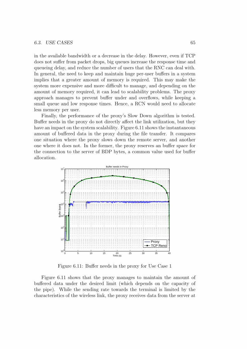
6.3. USE CASES 65
in the available bandwidth or a decrease in the delay. However, even if TCPdoes not suffer from packet drops, big queues increase the response time andqueueing delay, and reduce the number of users that the RNC can deal with.In general, the need to keep and maintain huge per-user buffers in a systemimplies that a greater amount of memory is required. This may make thesystem more expensive and more difficult to manage, and depending on theamount of memory required, it can lead to scalability problems. The proxyapproach manages to prevent buffer under and overflows, while keeping asmall queue and low response times. Hence, a RCN would need to allocateless memory per user.
Finally, the performance of the proxy’s Slow Down algorithm is tested.Buffer needs in the proxy do not directly affect the link utilization, but theyhave an impact on the system scalability. Figure 6.11 shows the instantaneousamount of buffered data in the proxy during the file transfer. It comparesone situation where the proxy slows down the remote server, and anotherone where it does not. In the former, the proxy reserves an buffer space forthe connection to the server of BDP bytes, a common value used for bufferallocation.
0 5 10 15 20 25 30 35 4010
0
101
102
103
104
105
106
107
Buffer needs in Proxy
Time (s)
Buf
fer
(byt
es)
ProxyTCP Reno
Figure 6.11: Buffer needs in the proxy for Use Case 1
Figure 6.11 shows that the proxy manages to maintain the amount ofbuffered data under the desired limit (which depends on the capacity ofthe pipe). While the sending rate towards the terminal is limited by thecharacteristics of the wireless link, the proxy receives data from the server at

66 CHAPTER 6. SIMULATIONS AND RESULTS
a higher speed. Hence, the amount of data that it would need to buffer if itdid not slow down the server would be unlimited, as it is shown in the graph.Note that the scale used is logarithmic, therefore the amount of buffereddata is approximately 100 times higher when the Slow Down algorithm isnot used. As in the case of the RNC, maintaining small buffers increases thenumber of users that the system can deal with.
6.3.2 Use case 2: Web browsing
In recent years, World Wide Web traffic has shown a huge growth, andnowadays it is one of the main contributors to Internet traffic. Web browsingmodelling has been subject of research for the past ten years, and there aremany publications focused on web users behavior. [34] proposes a model foruser decisions, based on large empirical studies on data provided by AmericaOn Line caching proxies. On the other hand, [35] shows another modelfocused on intra-site browsing, and presents web user behavior as dependenton many factors (such as the number of pages visited within the same site,as well as download time, repeat visits and others). [36] shows the influenceof Web page size and complexity on the total download time, and serverperformance.
For this thesis point of view, web browsing affects the performance ofTCP in two ways. First, web browsing implies the transfer of relativelysmall files. This means that, in the case of TCP, the connection spends mostof the time in Slow Start, hence the impact of Slow Start latency is greaterthan in the previous Use Case. Second, the amount of buffered data in theRNC significantly affects the response time. When a user clicks on a linkbefore the current page download is complete, there is no way to commandthe RNC to drop the queued packets belonging to a previous connection.These remaining packets from an already closed connection (“stale” data)slow down the establishment of the subsequent one, and increase the responsetime1.
In order to test both effects, two independent simulations were performed,based on the setups defined in figures 6.2 and 6.1, the bandwidth and delaysetting explained in Use Case 1, and using a bandwidth variation in thewireless link according to the following table:
In a general case, a web page comprises a base HTML file and a set ofobjects related to it. It is assumed that HTTP 1.1 protocol is used for webbrowsing, so a single persistent TCP connection is used to download the
1For this report, the response time is defined as the time that elapses since a link isclicked until the first data packet is being transmitted through the air interface.
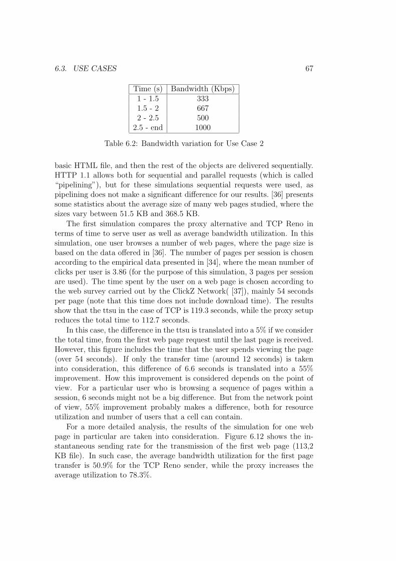
6.3. USE CASES 67
Time (s) Bandwidth (Kbps)1 - 1.5 3331.5 - 2 6672 - 2.5 500
2.5 - end 1000
Table 6.2: Bandwidth variation for Use Case 2
basic HTML file, and then the rest of the objects are delivered sequentially.HTTP 1.1 allows both for sequential and parallel requests (which is called“pipelining”), but for these simulations sequential requests were used, aspipelining does not make a significant difference for our results. [36] presentssome statistics about the average size of many web pages studied, where thesizes vary between 51.5 KB and 368.5 KB.
The first simulation compares the proxy alternative and TCP Reno interms of time to serve user as well as average bandwidth utilization. In thissimulation, one user browses a number of web pages, where the page size isbased on the data offered in [36]. The number of pages per session is chosenaccording to the empirical data presented in [34], where the mean number ofclicks per user is 3.86 (for the purpose of this simulation, 3 pages per sessionare used). The time spent by the user on a web page is chosen according tothe web survey carried out by the ClickZ Network( [37]), mainly 54 secondsper page (note that this time does not include download time). The resultsshow that the ttsu in the case of TCP is 119.3 seconds, while the proxy setupreduces the total time to 112.7 seconds.
In this case, the difference in the ttsu is translated into a 5% if we considerthe total time, from the first web page request until the last page is received.However, this figure includes the time that the user spends viewing the page(over 54 seconds). If only the transfer time (around 12 seconds) is takeninto consideration, this difference of 6.6 seconds is translated into a 55%improvement. How this improvement is considered depends on the point ofview. For a particular user who is browsing a sequence of pages within asession, 6 seconds might not be a big difference. But from the network pointof view, 55% improvement probably makes a difference, both for resourceutilization and number of users that a cell can contain.
For a more detailed analysis, the results of the simulation for one webpage in particular are taken into consideration. Figure 6.12 shows the in-stantaneous sending rate for the transmission of the first web page (113,2KB file). In such case, the average bandwidth utilization for the first pagetransfer is 50.9% for the TCP Reno sender, while the proxy increases theaverage utilization to 78.3%.

68 CHAPTER 6. SIMULATIONS AND RESULTS
0 1 2 3 4 5 60
200
400
600
800
1000
1200
Time (s)
Rat
e (K
bits
/s)
ProxyTCP RenoAvailable BW
Figure 6.12: Comparison of bandwidth utilization in terms of instantaneoustransmission rate for the first web page
In the case of the proxy, the whole file transfer is finished even before theReno sender achieves a reasonably high sending rate. This agrees with thefigures that show the average link utilization for the first web page: 50.9%for the Reno sender, and 78.3% in the case of the proxy. The reason for thisresult is that small files are specially affected by the Slow Start latency ofTCP, so the whole file transfer spends most of the time in this state. Thegraph shows that, while the proxy manages to adapt its transmission rate tothe link bandwidth, the Reno sender cannot keep up with the available rate.
The second simulation studies the response time when a user clicks ona different link before the previous page is completely downloaded. It isassumed that the user has enough information to decide whether to stay onthe page or not, once the base HTML file has been received. According to theperformance studies conducted in [36], the statistics show that for a 135 KBaverage page size, only 7.28% corresponds to the size of the base HTML file.In this simulation, the performance of the proxy and TCP Reno is compared(in terms of response time) when a user clicks on a different link after 9.8KB (out of 135 KB) have been received. In such case, the response time isclose to 45 milliseconds in both cases, although the ttsu (transfer of part ofthe first page, and complete second pages) is 4.53 seconds in the TCP Renocase, and 3.7 seconds with the proxy setup.
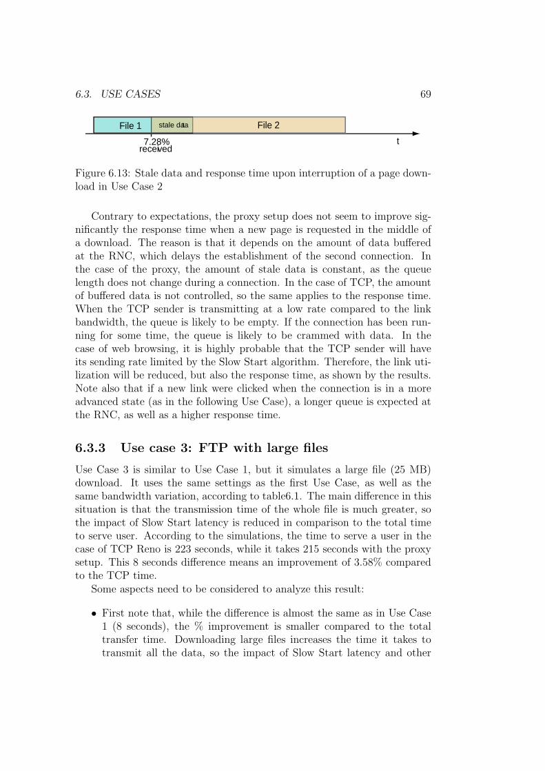
6.3. USE CASES 69
File 1 File 2
t7.28%
stale data
received
Figure 6.13: Stale data and response time upon interruption of a page down-load in Use Case 2
Contrary to expectations, the proxy setup does not seem to improve sig-nificantly the response time when a new page is requested in the middle ofa download. The reason is that it depends on the amount of data bufferedat the RNC, which delays the establishment of the second connection. Inthe case of the proxy, the amount of stale data is constant, as the queuelength does not change during a connection. In the case of TCP, the amountof buffered data is not controlled, so the same applies to the response time.When the TCP sender is transmitting at a low rate compared to the linkbandwidth, the queue is likely to be empty. If the connection has been run-ning for some time, the queue is likely to be crammed with data. In thecase of web browsing, it is highly probable that the TCP sender will haveits sending rate limited by the Slow Start algorithm. Therefore, the link uti-lization will be reduced, but also the response time, as shown by the results.Note also that if a new link were clicked when the connection is in a moreadvanced state (as in the following Use Case), a longer queue is expected atthe RNC, as well as a higher response time.
6.3.3 Use case 3: FTP with large files
Use Case 3 is similar to Use Case 1, but it simulates a large file (25 MB)download. It uses the same settings as the first Use Case, as well as thesame bandwidth variation, according to table6.1. The main difference in thissituation is that the transmission time of the whole file is much greater, sothe impact of Slow Start latency is reduced in comparison to the total timeto serve user. According to the simulations, the time to serve a user in thecase of TCP Reno is 223 seconds, while it takes 215 seconds with the proxysetup. This 8 seconds difference means an improvement of 3.58% comparedto the TCP time.
Some aspects need to be considered to analyze this result:
• First note that, while the difference is almost the same as in Use Case1 (8 seconds), the % improvement is smaller compared to the totaltransfer time. Downloading large files increases the time it takes totransmit all the data, so the impact of Slow Start latency and other

70 CHAPTER 6. SIMULATIONS AND RESULTS
TCP problems is reduced. From a user point of view, waiting 8 secondsin a 4 minutes download probably does not make a difference.
• Second, although one user may not be bothered by a 8 seconds dif-ference, it is important from the network point of view. One UMTSoperator is likely to be able to serve more users if the radio resourcesare fully utilized.
• Finally, it is important to note that, as in Use Case 1, this 8 seconds dif-ference is due to TCP’s initial Slow Start phase, the initial bandwidthvariation, and the delay introduced by the Exponential Backoff algo-rithm during the outage (see table 6.1). Use Case 3 assumes an initialvariation as in the first Use Case, one outage, and then a constant rateduring almost 4 minutes. It is highly unlike that the bandwidth wouldremain constant for such a long time, and more bandwidth variation (asin table 6.3) is expected during the download. We can roughly assumea 7 seconds difference between the proxy and TCP Reno ttsu for aninterval of bandwidth variation (according to table 6.3) and one out-age. Then, every time this situation is repeated during the connection,the difference will increase in 7 seconds. If the variation (or a simi-lar one) were repeated two times during the download, the differencewould be 14 seconds (6%), and so on. The second simulation confirmsthis assumption, where after a bandwidth variation as in table 6.3, thedifference in the ttsu for TCP Reno and the proxy setups is around13.1 seconds.
In order to check the effect of more bandwidth variation on the totaltransfer time, a second simulation is performed where the bandwidth variesaccording to the following scheme:
In this case, the ttsu is 220.5 seconds when the proxy is used, and 233.6in the case of TCP Reno.
However, when transmitting large files with TCP through wireless links, anew problem arises. TCP suffers from reduced buffers, as they lead to manypacket drops that cause the sender repeatedly reduce the transmission rate.Then, buffer allocation at the bottleneck (the RNC), as well as scalability,become an issue. Figure 6.14 shows variation with time of the the queuelength at the RNC, during the whole file transfer. It compares the length fora TCP Reno sender, as well as for a proxy setup. In this case, the maximumqueue length per connection at the RNC is limited to 25 packets. A simpleDrop-Tail queue is used, so subsequent packets arriving to a full queue aredropped.

6.3. USE CASES 71
Time (s) Bandwidth (Kbps)1 - 2.5 6672.5 - 3 5003 - 3.5 1000
3.5 - 8.5 08.5 - end 100041 - 42.5 66742.5 - 43 50043 - 43.5 1000
43.5 - 48.5 048.5 - end 1000
Table 6.3: Bandwidth variation for Use Case 3
Figure 6.14 shows that the proxy manages to maintain a constant queuelength independently of the network conditions and bandwidth variation.On the contrary, TCP increases its cwnd in spite of the limited bandwidth,and as a result the queue in the RNC is increased without control. Thissituation continues until the queue is full, and packets are dropped (queueoverflow). Then, TCP cuts the transmission rate to half, and the queue isdrained, leading to TCP’s typical sawtooth behavior, as shown in the graph.Whether a queue underflow will follow the overflow depends on the bufferlimit at the RNC, i.e., the moment when the first packet was dropped. Tosum up, the proxy also outperforms TCP in this case, as it manages tomaintain a reduced and controlled queue at the RNC, it keeps a reducedqueueing delay and response time, and it prevents buffer underflows (whichlead to link under-utilization).
The last simulation aims to study the effect of maximum queue size at theRNC. In this case, the allocated buffer at the bottleneck is set to 10 packets,and the results are presented in figure 6.15. The graph on the left shows theinstantaneous queue length for both the proxy and TCP Reno setups, whilethe right one represents the transmission rate, compared with the availableBW assigned to the connection every instant.
Figure 6.15 shows that, while the proxy maintains a constant queue lengthas well as maximum transmission rate, TCP suffers from many overflows,which lead to subsequent buffer underflows. The right graph shows thatthese underflows are translated into a reduction of the sending rate, belowthe link bandwidth, which leads to poor link utilization. On the contrary,the proxy manages to maintain an optimal (close to 100%) link utilization.

72 CHAPTER 6. SIMULATIONS AND RESULTS
0 10 20 30 40 500
5
10
15
20
25
30
Time (s)
Que
ue (
pkts
)
ProxyTCP Reno
Figure 6.14: Comparison of RNC queue length variation during a large filetransfer in use case 3
ttsu (s) % usedUseCase 1 TCP Reno 47.3 77%
Proxy 39.2 98.3%UseCase 2 TCP Reno 3.9 50.9%
Proxy 3.0 78.3%UseCase 3 TCP Reno 233.6 61%
Proxy 220.5 98%
Table 6.4: Summary of results for the three Use Cases

6.3. USE CASES 73
0 10 20 30 40 50 60 700
2
4
6
8
10
12
14
16
18
20
Time (s)
Que
ue (
pkts
)
0 10 20 30 40 50 60 700
200
400
600
800
1000
1200
Time (s)
Rat
e (K
bits
/s)
ProxyTCP RenoAvailable BW
ProxyTCP Reno
Figure 6.15: Effect of reduced RNC buffer space on the connection through-put in terms of RNC queue length and instantaneous transmission rate
74 CHAPTER 6. SIMULATIONS AND RESULTS

Chapter 7
Conclusions and outlook
In this report, a proxy-based solution to improve the performance of TCPon 3G networks has been presented. First, the main problems of TCP overwireless links have been identified, and some proposed solutions have beenstudied. Previous solutions have focused on some of the problems, but noneof them addresses all the problems in one. Moreover, most of the times theproposed solutions imply a modification of one or both endpoints. The RadioNetwork Feedback consists in a proxy-based split-connection solution, whichaims at addressing all the problems at once, and without the need to changethe remote servers nor the mobile terminals. This can be achieved if thetransport agent at the proxy is aware of the varying wireless link conditions,and modifies its congestion window in order to adapt its transmission rateto the bandwidth changes. It takes advantage of the network informationreceived from the RNC, while TCP needs to take conservative measures, dueto the fact that it can only count on end-to-end information.
In order to compare the proxy setup to TCP Reno, a set of simulationshave been performed. General performance aspects and performance in prac-tical situations have been tested and analyzed. The simulations results haveshown that it is possible to significantly improve the link utilization and ef-ficiency of a TCP connection, as well as reduce buffer needs and queuingdelays. The presented Radio Network Feedback solution remarkably out-performs a common TCP version such as TCP Reno. The proxy reducesthe Slow Start latency, increases the link utilization and properly adapts toabrupt bandwidth changes. It can also deal with delay variation, and reducesbuffer needs at intermediate elements as well as queuing delays.
Performance improvements can be measured in terms of end user’s expe-rience, as well as from the mobile operator’s point of view. End users areinterested in reduced latency and response times, and the possibility of enjoy-ing interactive and real time services, which is directly related to end-to-end
75

76 CHAPTER 7. CONCLUSIONS AND OUTLOOK
delay and delay variation. On the other hand, operators are interested infully utilizing the scarce and expensive radio resources, supporting the max-imum number of users per cell, and making their systems scalable. To sumup, some performance improvements that are relevant to operators might notbe regarded the same way by end users, but all of them are important forthe overall 3G system performance.
Using a proxy that resides in the UMTS Core Network provides the mobileoperators with complete control over the adaptation, and allows them tomake any modifications to the TCP agent used towards the terminals. Thisway, the necessary changes are limited to the operator’s network, while anyother elements may remain unchanged. Using a proxy allows to perform allthe adaptation without the need to change the remote servers, nor the mobileterminals.
For the simulations, Drop-Tail buffers have been used. In addition, itwould be interesting to study and compare the proxy solution and TCP withmore advanced buffer management techniques. It could also be interestingto test the system with many users, in order to study the effect of a highernetwork load. On the other hand, a simple algorithm has been used for theclosed-loop queue control, but it would be desirable to develop more advancedalgorithms, in order to get the most out of the RNC queue information.

Bibliography
[1] D.A.R.P.A. The transmission control protocol. RFC 0793, September1981.
[2] J.F. Kurose and K.W. Ross. Computer Networking: A top-down ap-proach featuring the Internet. Addison-Wesley, second edition, 2003.
[3] S. Chemiakina and J. Petersson. Radio network based adaptationmethod for packet switched services over 3G mobile systems. IST Mobileand Wireless Communications, June 2004.
[4] V. Jacobson and R. Braden. TCP extensions for long-delay paths. RFC1072, October 1988.
[5] V. Jacobson, R. Braden, and L. Zhang. TCP extension for high-speedpaths. RFC 1185, October 1990.
[6] V. Jacobson, R. Braden, and D. Borman. TCP extensions for highperformance. RFC 1323, May 1992.
[7] M. Mathis, J. Mahdavi, S. Floyd, and A. Romanow. TCP selectiveacknowledgement options. RFC 2018, October 1996.
[8] Lawrence S. Brakmo and Larry L. Peterson. TCP vegas: End to endcongestion avoidance on a global internet. IEEE Journal on SelectedAreas in Communications, 13(8):1465–1480, 1995.
[9] Saverio Mascolo, Claudio Casetti, Mario Gerla, M. Y. Sanadidi, and RenWang. TCP westwood: Bandwidth estimation for enhanced transportover wireless links. In Mobile Computing and Networking, pages 287–297, 2001.
[10] Saverio Mascolo, Luigi Alfredo Grieco, Giovanni Pau, Mario Gerla, andClaudio Casetti. End-to-end bandwidth estimation in TCP to improvewireless link utilization.
77

78 BIBLIOGRAPHY
[11] Mario Gerla, M. Y. Sanadidi, Ren Wang, and Andrea Zanella. TCPwestwood: Congestion window control using bandwidth estimation.
[12] C. Casetti, M. Gerla, S. Lee, S. Mascolo, and M. Sanadidi. TCP withfaster recovery. MILCOM, October 2000.
[13] Hari Balakrishnan, Srinivasan Seshan, and Randy H. Katz. Improvingreliable transport and handoff performance in cellular wireless networks.ACM Wireless Networks, 1(4), 1995.
[14] M. Allman, S. Floyd, and C. Partridge. Increasing TCP’s initial window.RFC 3390, October 2002.
[15] Ren Wang, Giovanni Pau, Kenshin Yamada, M.Y. Sanadidi, and MarioGerla. TCP startup performance in large bandwidth delay networks.IEEE-INFOCOM, 2003.
[16] V. Padmanabhan and R. Katz. Tcp fast start: a technique for speedingup web transfers. In Globecom 1998 Internet Mini-Conference. IEEE,1998.
[17] Y. Nishida. Smooth slow-start: refining TCP slow-start for large-bandwidth with long-delay networks. In 23rd Annual Conference onLocal Computer Networks, pages 52–60, October 1998.
[18] K. Brown and S. Singh. M-TCP: TCP for mobile cellular networks.ACM Computer Communication Review, 27(5), 1997.
[19] T. Goff, J. Moronski, D.S. Phatak, and V. Gupta. Freeze-TCP: a trueend-to-end TCP enhancement mechanism for mobile environments. InNineteenth Annual Joint Conference of the IEEE Computer and Com-munications Societies, volume 3, pages 1537 – 1545. IEEE-INFOCOM,March 2000.
[20] M. Choon Chan and R. Ramjee. TCP/IP performance over 3G wirelesslinks with rate and delay variation. MOBICOM, September 2002.
[21] M. Choon Chan and R. Ramjee. Improving TCP/IP performance overthird generation wireless networks. IEEE-INFOCOM, 2004.
[22] D. Dutta and Y. Zhang. An active proxy based architecture for TCPin heterogeneous variable bandwidth networks. IEEE GLOBECOM,November 2001.
BIBLIOGRAPHY 79
[23] L. Kalampoukas, A. Varma, and K.K. Ramakrishnan. Explicit windowadaptation: a method to enhance TCP performance. In IEEE/ACMTransactions on Networking, volume 10, pages 338 – 350. IEEE, June2002.
[24] Michael Savoric. Fuzzy explicit window adaptation: using router feed-back to improve TCP performance. TKN Technical Reports Series, July2004.
[25] D. Dutta and Y. Zhang. An early bandwidth notification (EBN) ar-chitecture for dynamic bandwidth environment. In IEEE InternationalConference on Communications, volume 4. IEEE, April 2002.
[26] J. Krause. High speed downlink packet access: Iub/iur protocol aspects(release 5). 3GPP Specification, June 2002.
[27] F. Gunnarsson and F. Gustafsson. Power control in wireless communi-cations networks - from a control theory perspective.
[28] T.E. Kolding, F. Frederiksen, and P.E. Mogensen. Performance aspectsof WCDMA systems with high speed downlink packet access (HSDPA).In 56th Vehicular Technology Conference, volume 1, pages 477–481.IEEE, September 2002.
[29] M. Dottling, J. Michel, and B. Raaf. Hybrid ARQ and adaptive modula-tion and coding schemes for high speed downlink packet access. In The13th IEEE International Symposium on Personal, Indoor and MobileRadio Communications, volume 3, pages 1073–1077. IEEE, September2002.
[30] UMTS forum home page. http://www.umts-forum.org.
[31] L. Brakmo, S. O’Malley, and L. Peterson. TCP vegas: New techniquesfor congestion detection and avoidance. In Proceedings of the SIGCOMM’94 Symposium, pages 24–35, August 1994.
[32] J. Mo, R.J. La, V. Anantharam, and J. Walrand. Analysis and com-parison of TCP reno and vegas. In Eighteenth Annual Joint Conferenceof the IEEE Computer and Communications Societies, volume 3, pages1556–1563. IEEE, March 1999.
[33] The network simulator 2. http://www.isi.edu/nsnam/ns/, August 2004.

80 BIBLIOGRAPHY
[34] Bernardo A. Huberman, Peter L. T. Pirolli, James E. Pitkow, and Ra-jan M. Lukose. Strong regularities in World Wide Web surfing. Science,280(5360):95–97, 1998.
[35] R.E. Bucklin and C. Sismeiro. A model of Web Site browsing behaviorestimated on clickstream data. Journal of Marketing Research, XL:249–267, August 2003.
[36] C. Hava Muntean, J. McManis, and J. Murphy. The influence of Webpage images on the performance of Web servers. Lecture Notes in Com-puter Science, 2093:821–??, 2001.
[37] The ClickZ network. http://www.clickz.com/stats/sectors/traffic patterns/,November 2004.
[38] M. Sagfors, R. Ludwig, M. Meyer, and J. Peisa. Buffer managementfor rate-varying 3G wireless links supporting TCP traffic. In VehicularTechnology Conference, volume 1, pages 675 – 679. IEEE, April 2003.