Radio-Frequency Interference (RFI) From Extra-High-Voltage (EHV) Transmission Lines

Patrick C. Crane 22 March 2010

1. Introduction The subject of radio-frequency interference (RFI) generated by high-voltage transmission lines has long been of both academic and commercial interest because of concerns about static on AM radio. Today audible noise is of greater concern because many states, counties, and municipalities have noise ordinances and transmission lines are designed to reduce audible noise, while people now expect static on AM radio (Chartier 2009). The subject is of interest today because of the proliferation around the world of low-frequency radio telescopes – including the Low Frequency Array (LOFAR), the Giant Metrewave Radio Telescope (GMRT), the Murchison Widefield Array (MWA), and the Long Wavelength Array (LWA), which is particular interest to the author. The present discussion will concern high-voltage alternating-current (HVAC) transmission lines; high-voltage direct-current (HVDC) transmission lines will be addressed in Appendix A. As described by Pakala and Chartier (1971) power lines are divided into two classes with respect to radio noise: (1) lines with voltages below 70 kV and (2) lines with voltages above 110 kV. Lines in the first class in general exhibit only gap-type discharges and lines in the second class principally exhibit corona discharge. Gap-type discharges are essentially a maintenance issue; corona discharges are a design issue. Extra-high-voltage (EHV) transmission lines have operating voltages of 345 kV or greater. The possibility of interference from such a transmission line first impinged significantly upon radio astronomy (in the United States, at least) in 1984 when the El Paso Electric Company proposed building a 345-kV transmission line from Red Hill, NM to Deming, NM which would run east along US60 to its junction with NM78 (now NM52) and then south along NM78. This route would have crossed both the north and east arms about two miles from the center of the Very Large Array (VLA) radio telescope. In response, the Bureau of Land Management (BLM) hired Vernon L. Chartier of the Bonneville Power Administration (BPA) as a consultant to study the problem and recommend minimum separation distances for the VLA and for the Very Long Baseline Array (VLBA) radio telescope, construction of which began in 1985. Mr. Chartier was well qualified for the task as the Chief High Voltage Phenomena Engineer of BPA’s Division of Laboratories with many years of research in the field. He is still active and when I contacted him (vlchartier@ieee.org), he provided more recent references. Among them is the EPRI Red Book (2008) which is published by the Electric Power Research Institute, Inc. (EPRI); Mr. Chartier sent me the small number of relevant pages because the Red Book sells for $5000. The EPRI is an independent nonprofit

1

organization that conducts research and development relating to the generation, delivery and use of electricity for the benefit of the public. The Red Book (2008) recognizes the BPA method because The most complete empirical method for predicting EMI above 30 MHz is the method developed by the Bonneville Power Administration (Chartier 1983). The BPA method was first developed to predict TVI from overhead lines during rain, but the method has been expanded so that EMI above 30 MHz can be calculated at any frequency, at any distance from the line, at any antenna height, for any bandwidth, and for any detector. Furthermore, it is “the one method that is useful for EMI predictions between 30 and 1000 MHz” and “the most complete empirical method for predicting EMI above 30 MHz.” The BPA model also has been recognized by the International Council on Large Electric Systems (CIGRE, 1996), which is one of the leading worldwide organizations on electric power systems. 2. What Is Corona? Hubbell Power Systems, Inc. (2004) has produced a clear and concise report on corona with the title “What Is Corona?” which is available on the World Wide Web. This report defines corona in the following terms: Corona is a luminous discharge due to ionization of the air surrounding a conductor around which exists a voltage gradient exceeding a certain critical value, based upon IEEE Std 539-1990 (IEEE Corona and Field Effects Subcommittee, 1991) as applied to transmission-line conductors. Or in more physical terms: The corona discharges observed at the surface of a conductor are due to the formation of electron avalanches which occur when the intensity of the electric field at the surface of a conductor exceeds a certain critical value. Furthermore, Any defect on the conductor[,] which projects however slightly above the nominal conductor surface, increases the field intensity in its immediate vicinity...Water drops on the conductor surface provide a multiplicity of projections from which corona discharges can originate...A weathered ACSR conductor generally has a multiplicity of tiny surface defects which project above the nominal surface of the conductor. The presence of corona manifests itself primarily in three ways:

2

1. “Visual corona” – violet-colored light coming from the regions of electrical overstress. Daytime corona cameras and ultraviolet cameras both are used to inspect transmission lines for corona. 2. “Audible corona” – a hissing or frying sound when corona is present. 3. Radio noise – apparently this is the most serious manifestation from the point-of-view of the power company (for radio astronomers, too) because its effects have the longest range. The phenomena associated with corona have been described quantitatively by Chartier (1983): radio noise (RI) over the frequency range 0.1-20 MHz (i.e., AM radio, ham radio); television interference (TVI) over the frequency range 10-1000 MHz, which includes VHF and UHF television and FM radio and, coincidentally, is measured in the radio-astronomy allocation 73.0-74.6 MHz because of the absence of interference; audible noise (AN); and ozone (concentration C). The total power loss per meter of conductor is identified as the corona losses (CL). The presence of more surface defects produces higher levels of corona and related phenomena. Indulkar (2004) discusses the effects of such surface irregularities on the threshold voltage for the onset of corona. He reports that this voltage is directly proportional to an irregularity factor, m0 (0<m0≤1): 1 for smooth, polished, solid, cylindrical conductors; 0.93-0.98 for weathered, solid, cylindrical conductors; 0.87-0.90 for weathered conductors with more than seven strands; and 0.80-0.87 for weathered conductors with up to seven strands. Finally, the Introduction states that corona from EHV transmission lines is primarily a design problem. While that is true – from the point-of-view of a radio astronomer, corona can be a maintenance issue because of such problems as degraded or damaged insulators; contamination with coastal salt, industrial vapors and dust, cement dust, road salt, tire dust and vehicle emissions; agricultural dusts and fertilizers; improper design and/or installation; and loose hardware. 3. Television Interference (TVI) As stated above the method developed by the Bonneville Power Administration (BPA) is the most complete empirical method for predicting radio-frequency interference (RFI) above 30 MHz. The BPA calculation of TVI/phase for a CISPR quasi-peak detector from corona discharge is given by Equation 9.6-4 in EPRI (2008): TVI/phase = 10 + TVIV(E) + TVIS(d) + TVIf + TVIA+ TVID(L), (1) where

3

TVI/phase = electric field (dBμV/m), measured during steady rain with an

IEC/CISPRQuasi-Peak (QP) detector with a 1-ms charge time constant, a 550-ms discharge time constant, and 6-dB bandwidth of 120 kHz, for a single phase,

E = conductor surface voltage gradient (kV/cm), d = subconductor diameter (cm), f = frequency (MHz), A = altitude above sea level (km), L = distance between antenna and phase (m). Individual terms will be discussed in the following sections. 3.1. Conductor Surface Voltage Gradient TVIV(E) = 120*log(E/16.3), (2) where E = conductor surface voltage gradient (kV/cm). The conductor surface voltage gradient is the single most important factor in determining the corona performance of a high-voltage transmission line. This is indicated by the multiplicative factor of 120 in front of the appropriate (second) term in Equation (1); the multiplicative factors for other terms are 40, 20, and 1. If E changes by a factor of ±2, the TVI will change by ±36 dB. It is so important, also, because its value is entirely a design issue. Therefore, the calculation of its value has long and widely been the subject of investigation. A survey of methods used for such calculations (as of 1979) was published by the IEEE Corona and Field Effects Subcommittee (1979). Seventeen techniques were applied to multiple extra-high-voltage (EHV, ≥345 kV) transmission-line configurations. Empirical techniques were found to agree with exact solutions to within a few percent, so that when applied in the field the overall uncertainty was less than ten percent. A further uncertainty may arise from the definition of the conductor surface voltage gradient; the three definitions used in the survey include the average bundle gradient (A), the average maximum bundle gradient (AM), and the maximum bundle gradient (MB). As a practical matter, Table I of the paper provides parameters for EHV transmission lines with operating voltages of 345 kV, 500 kV, 765 kV, 1100 kV, and 2000 kV (AC) and ±375 kV and ±1000 kV (DC). The computed gradients are listed in Table II. Participant No. 4 is Vernon L. Chartier and he reports only the results of an AM calculation. By 1979, such calculations had migrated to the digital computer and had expanded in capability and complexity. One can see an earlier version of the BPA calculation, suitable for manual calculation, in Pakala and Taylor (1968). I have implemented in IDL (Appendix B) the 1991 version of the Fortran code used by V. L. Chartier (Participant No. 4) for the 1979 paper and obtained exactly his results.

4

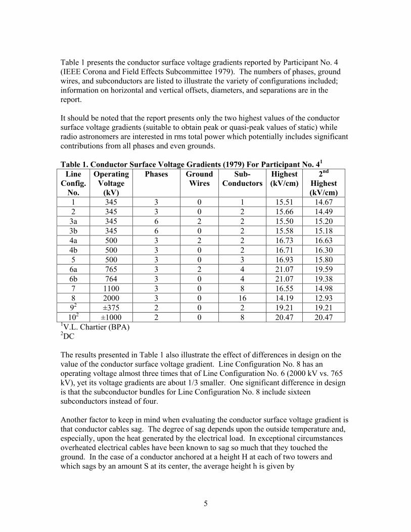
Table 1 presents the conductor surface voltage gradients reported by Participant No. 4 (IEEE Corona and Field Effects Subcommittee 1979). The numbers of phases, ground wires, and subconductors are listed to illustrate the variety of configurations included; information on horizontal and vertical offsets, diameters, and separations are in the report. It should be noted that the report presents only the two highest values of the conductor surface voltage gradients (suitable to obtain peak or quasi-peak values of static) while radio astronomers are interested in rms total power which potentially includes significant contributions from all phases and even grounds. Table 1. Conductor Surface Voltage Gradients (1979) For Participant No. 41

Line Config.

No.

Operating Voltage

(kV)

Phases Ground Wires

Sub-Conductors

Highest (kV/cm)

2nd Highest (kV/cm)

1 345 3 0 1 15.51 14.67 2 345 3 0 2 15.66 14.49 3a 345 6 2 2 15.50 15.20 3b 345 6 0 2 15.58 15.18 4a 500 3 2 2 16.73 16.63 4b 500 3 0 2 16.71 16.30 5 500 3 0 3 16.93 15.80 6a 765 3 2 4 21.07 19.59 6b 764 3 0 4 21.07 19.38 7 1100 3 0 8 16.55 14.98 8 2000 3 0 16 14.19 12.93 92 ±375 2 0 2 19.21 19.21 102 ±1000 2 0 8 20.47 20.47

1V.L. Chartier (BPA) 2DC The results presented in Table 1 also illustrate the effect of differences in design on the value of the conductor surface voltage gradient. Line Configuration No. 8 has an operating voltage almost three times that of Line Configuration No. 6 (2000 kV vs. 765 kV), yet its voltage gradients are about 1/3 smaller. One significant difference in design is that the subconductor bundles for Line Configuration No. 8 include sixteen subconductors instead of four. Another factor to keep in mind when evaluating the conductor surface voltage gradient is that conductor cables sag. The degree of sag depends upon the outside temperature and, especially, upon the heat generated by the electrical load. In exceptional circumstances overheated electrical cables have been known to sag so much that they touched the ground. In the case of a conductor anchored at a height H at each of two towers and which sags by an amount S at its center, the average height h is given by

5

h = H – ⅔ S. (3) This is the value that should be used to calculate the conductor surface voltage gradient. 3.2. Subconductor Diameter TVIS(d) = 40*log(d/3.04), (4) where d = subconductor diameter (cm). The subconductor diameter affects the TVI in two ways, which tend to offset each other. The first is indirectly through its effects on the values of the conductor surface voltage gradients; the larger the diameter, the lower the values. For example, Chartier (1984) reported that increasing the subconductor diameter from 1.108 inches to 1.196 would decrease the values of the conductor surface voltage gradients by 6 percent; the corresponding decrease in the value of the second term in Equation (1) would be 3.3 dB or 53 percent. The second way is directly through the third term in Equation (1). The increase in subconductor diameter mentioned in the previous paragraph would increase the TVI by 1.4 dB or 37 percent. 3.3. Frequency Dependence TVIf = 20*log(75/f), (5) where f = frequency (MHz). The data supporting this correction are discussed in Pakala and Chartier (1971). The measurements presented in their Figures 10 and 11 were obtained in fair weather at a reference distance of 200 feet (61 m) from the outer conductor of transmission lines with voltages of 244 kV, 345 kV, 525 kV, and 735 kV. In theory and practice this simple behavior breaks down at larger distances. At low frequencies of interest to the LWA and the VLA (13.385, 25.610, 37.875, 73.8, 151.525, 325.3, 408.05, and 611.0 MHz), the contributions from this term are 15, 9.3, 5.9, 0.1, -6.1, -13, -15, and -18 dB, respectively. 3.4. Altitude Dependence TVIA = (A/0.3), (6)

6

where A = altitude (km). This term reflects Paschen’s Law which states that at typical atmospheric pressures the breakdown voltage for corona discharge decreases as the pressure (density) decreases (which occurs naturally as the altitude increases). This form of the correction was derived from measurements of the radio noise (RI) produced by low-altitude (195 m) and high-altitude (3200 m) EHV transmission lines. It was later shown to describe the behavior of television interference (TVI) by Chartier et al. (1987). This term is relatively unimportant, since a change in altitude from sea level to 3 km results in an adjustment of only 10 dB. 3.5. Lateral Attenuation TVID(L) = 20*log(L0/L), for L and L0 ≤ Lc, (7a) = 20*log(L0/Lc) + 40*log(Lc/L), for L ≥ Lc and L0 ≤ Lc, (7b) = 20*log(Lc/L) + 40*log(L0/Lc), for L ≤ Lc and L0 ≥ Lc, (7c) = 40*log(L0/L), for L and L0 ≥ Lc, (7d)

where ha = antenna height (m), H = conductor height (m), λ = wavelength (m), L = lateral distance between phase and antenna (m), L0 = 61 m (200 ft), reference lateral distance, Lc = 12 ha H λ-1, changeover distance. This relatively simple expression accounts for the lateral attenuation of TVI in the BPA method for corona discharge from EHV transmission lines. Nominally, it applies to frequencies between 30 MHz and ≥1000 MHz; at distances of interest to us it probably applies to frequencies ≥10 MHz (Chartier 2009). This expression does not depend explicitly upon frequency but an implicit dependence is introduced by the changeover distance, Lc, which marks the boundary between near-field and far-field behavior. At frequencies of interest to the LWA (13.385, 25.610, 37.875, and 73.8 MHz), the values of the changeover distance are 16.7 m, 32.0 m, 47.4 m, and 92.3 m, respectively. The lateral attenuation is normalized to unity (0 dB) at L0 independent of frequency and the transition from near-field to far-field behavior (L-2 to L-4) occurs at Lc. Consequently, at lower frequencies for which L ≥ L0 ≥ Lc and at the large distances of interest to us, we have

7

TVID(L) = 40*log(L0/L), (8a) which is frequency independent. On the other hand, at higher frequencies for which L ≥ Lc ≥ L0 and at the same large distances, we have TVID(L) = 20*log(L0/Lc) + 40*log(Lc/L), (8b) which is systematically greater than the prior result (since Lc ≥ L0) and frequency-dependent through the presence of Lc. These behaviors are illustrated in Figure 1. However, if the distances are normalized to the value of Lc at 75 MHz: L75 = 12*106 ha H f c-1, (9) the sum of Equations (5) and (8b) can be simplified to TVIf + TVID(L) = 20*log(L0/L75) + 40*log(L75/L), L ≥ Lc ≥ L0. (10) Surprisingly, as long as L ≥ Lc ≥ L0, the TVI/phase is independent of frequency, which is apparent in Figures 2, 3, and 4. The propagation of radio waves over a finitely conducting plane was first addressed by Sommerfeld (1909). These results were simplified for engineering work (Norton 1936, 1937) and extended eventually to the case of the finitely conducting spherical Earth (Norton 1941). Additional simplifications are provided by Pakala and Chartier (1971). I have not determined the provenance of Equation (4) but it is accepted by the domestic (EPRI 2008) and international (CIGRE 2000) electric power industries. Equation (4) applies to distances between approximately 61 m and 15000 m. At shorter distances interference between the space wave (itself a combination of direct and ground-reflected waves), the surface wave, the induction field, and the electrostatic field predominates – all propagating over a finitely conducting earth. At larger distances the curvature of the earth is important as is the variation of atmospheric refraction with altitude. 4. Detector, Bandwidth, and Power Equation (1) is based upon a CISPR quasi-peak (QP) detector with a bandwidth of 120 kHz. However, in practice, a different detector and different bandwidth may be used; the following conversion procedure originated with Chartier (1988). Corrections to other detectors and bandwidths are given in Tables 2 and 3, respectively, which are based upon Table 9.6-1 and Equations 9.6-5, 9.6-6, and 9.6-7 in the EPRI Red Book (2008).

8

TVI/phase in Equation (1) is an electric field whereas radio astronomers measure noise power. The steps in making the conversion from TVI (dBμV/m) to noise power P(dBW/m2/Hz) are (1) Convert from dBμV to dBV Correction = -120 dB. (11) (2) Convert from quasi-peak electric field to rms electric field Correction = -10 dB. (12) (3) Convert from a bandwidth of 120 kHz to a bandwidth of 1 Hz Correction = 10*log(1/120000) dB = -50.8 dB. (13) (4) Convert from rms electric field to noise power, which is done via P = E2/Z, (14) where P = noise power (W/m2/Hz), E = rms noise voltage (V/m/Hz1/2), Z = impedance of free space (377 Ω). Or 10*log[P(W/m2/Hz)] = 20*log[E(V/m/Hz1/2)] – 10*log(377), (15) P(dBW/m2/Hz) = E(dBV/m/Hz1/2) - 25.8 dB. (16) Finally, P(dBW/m2/Hz) = TVI(dBμV/m) – 206.6 dB. (17) Table 2. Corrections from QP to Other Detectors Detector Correction Quasi-Peak +0 dB Peak +5 dB RMS -10 dB Table 3. Bandwidth Corrections Detector Correction1 (ΔEpk) Quasi-Peak +0 dB Peak 20 log (BW/BW0) dB

9

RMS 10 log (BW/BW0) dB Average 10 log (BW/BW0) dB 1BW0 = 120 kHz 5. Operating Voltages Extra-high-voltage (EHV) transmission lines are labeled by voltages of 345 kV, 500 kV, 765 kV, 1100 kV, and even 2000 kV. But these voltages are only nominal. The actual operating voltages may be significantly higher; they are set by the individual utilities and will vary during the day as the nature of the load changes. There are, however, standards for the maximum voltages which manufacturers use to design and build the high-voltage equipment. The maximum extra-high voltages as established by the American National Standards Institute (ANSI C84.1-2006) are listed in Table 4; I found them listed in the IEEE Dictionary (IEEE 100). Table 4. Operating Voltages for EHV Transmission Lines1

Nominal (kV) Actual (kV)2 Maximum (kV) 345 ~350 362 500 ~535 550 765 … 800 1100 … 1200

1ANSI C84.1-2006 2Bonneville Power Administration It should be noted that operating voltages are rms phase-to-phase while the voltages used to calculate voltage gradients are rms line-to-ground; the latter are thus a factor of 31/2 smaller than the former. 6. Weather The altitude dependence discussed above is a simple example of the effects of the environment on TVI. More generally, weather has significant, but highly variable, effects. For example, according to Chartier (2009), a typical plot of an all-weather RI distribution is the superposition of three distinct Gaussian distributions: (1) high values during mean rainy weather (i.e., conductors thoroughly wet), (2) low values during mean fair weather, and (3) a transition distribution between measurable rain and fair weather - i.e., when the conductors are wet with dew, fog, light snow, and after rain - or in the presence of pollution caused by industry, farmers plowing their fields, etc. The BPA method calculates the TVI level during mean rainy weather but in very heavy rain the TVI level may be even higher (Pakala and Chartier 1971; Chartier 2009). Table 5. Adjustment for Weather Conditions

Weather Condition Adjustment Heavy Rain +5 dB

10

Mean Rainy Weather 0 dB Mean Fair Weather -25 dB

7. Thresholds for Harmful Interference In the United States, electromagnetic interference from power transmission systems is governed by the Federal Communications Commission (FCC) Rules and Regulations presently in existence (FCC, 1988). A power transmission system falls into the FCC category of “incidental radiation device,” which is defined as “a device that radiates radio frequency energy during the course of its operation although the device is not intentionally designed to generate radio frequency energy.” Such a device “shall be operated so that the radio frequency energy that is emitted does not cause harmful interference. In the event that harmful interference is caused, the operator of the device shall promptly take steps to eliminate the harmful interference.” For purposes of these regulations, harmful interference is defined as: “any emission, radiation or induction which endangers the functioning of a radio navigation service or of other safety services or seriously degrades, obstructs or repeated interrupts a radio communication service operating in accordance with this chapter” [FCC 1988]. This statement is reproduced from the Final Environmental Impact Statement for the Klondike III/Biglow Canyon Wind Integration Project (BPA 2006). The frequency range (10-88 MHz) of the LWA includes five allocations for radio astronomy; six other allocations are (or eventually may be) of interest to the VLA (Table 6). Table 6. Low-Frequency Allocations for Radio Astronomy Frequency Range Description (U.S.) 13360-13410 kHz Primary 25550-25670 kHz Primary 37.5-38.0 MHz Secondary, Land Mobile Primary 38.0-38.25 MHz Primary, Shared with Fixed and Mobile 73.0-74.6 MHz Primary 150.05-153.0 MHz Fixed, Mobile, and Land Mobile Primary* 322.0-328.6 MHz Footnote, Fixed and Mobile Primary* 406.1-410.0 MHz Primary, Shared with Fixed and Mobile 608.0-614.0 MHz Primary, Shared with Land Mobile 1400.0-1427.0 MHz Primary, Shared with Earth-Exploration Satellite

(passive) and Space Research (passive) *Radio Astronomy Primary Outside U.S. Twenty-five years ago it was recognized that synthesis-imaging arrays were intrinsically less sensitive to radio-frequency interference (RFI) than single radio telescopes that operate in total-power mode. In the case of a connected-element array fringe-frequency averaging and broadband decorrelation (Thompson 1982) may reduce the sensitivity to RFI significantly [see Figure 15.2 in Thompson, Moran, and Swenson (2001)]. In the

11

case of the VLA, in particular, these effects reduce its sensitivity to RFI by 15 dB, 19 dB, and 22 dB at 73.8 MHz, 325 MHz, and 1413.5 MHz, respectively (Crane 1985). However, what may be overlooked is that radio-astronomical arrays – such as the LWA – today and in the future need not be used exclusively for synthesis imaging. Indeed, one need only look at the science proposed for the first station of the LWA (LWA-1) to understand how erroneous that view is – pulsar spectra, “giant” pulses, scintillation and scattering effects; all-sky monitoring for transient events; low-frequency radio recombination lines; ionospheric-transparency events; ionospheric scintillation; frequency structure of solar and Jovian radio bursts; interplanetary scintillation. And, because multiple, independently tuned and pointed beams will be provided, both interferometric and total-power observations likely will occur simultaneously. Consequently, the appropriate protection criteria for the LWA are those recommended by the International Telecommunications Union (ITU) for a radio telescope operating in total-power mode in “ITU-R Recommendation RA.769-2: Protection Criteria for Radioastronomical Measurements” (ITU 2003): The harmful interference level is that level of interference which equals 0.1 of the rms noise level which sets the fundamental limit of the data. The corresponding spectral power flux density, ΔSH (Wm-2Hz-1), is given by ΔSH = 0.4πf2kTS(Bt)-1/2(c2Gs)-1, (18) where f is the observing frequency; k, Boltzman’s constant; TS, the system temperature; B, the observing bandwidth; c, the speed of light; Gs, the gain, with respect to an isotropic antenna (λ2/4π), of the antenna in the direction of the arrival of the interfering signal; and t, the total integration time. RA.769-2 adopts a total integration time of 2000 seconds, which is intermediate between short observations of time-varying phenomena and deep spectral-line observations. An antenna gain Gs of 0 dBi is adopted as a compromise between the high gain of the main beam and the low gain of the distant sidelobes. The system temperature, TS, is the sum of the antenna noise temperature, TA, and the receiver noise temperature, TR, or TS = TA + TR. (19) The Galactic background dominates the antenna temperatures at low frequencies; RA.769-2 uses the minimum temperatures observed at the North Galactic Pole in its calculations. The minimum temperature for 37.875 MHz was provided by Emil Polisensky (2009) using his program LFmap (Polisensky 2007). Table 7. Threshold Levels of Harmful Interference (RA.769-2) Center Frequency

fc (MHz)

Assumed Bandwidth

Δf (MHz)

Minimum Antenna Noise Temperature

TA (K)

Receiver Noise Temperature

TR (K)

Spectral pfd ΔSH

(dB(Wm-2Hz-1))

13.385 0.05 50000 60 -248 25.610 0.12 15000 60 -249 37.875 0.75 4000* 60 -255

12

73.8 1.6 750 60 -258 151.525 2.95 150 60 -259 325.3 6.6 40 60 -258 408.05 3.9 25 60 -255 611.0 6.0 20 60 -253 1413.5 27.0 12 10 -255

*Polisensky (2009) The thresholds of harmful interference derived in RA.769-2 are summarized in Table 7. ΔSH is fairly constant between 13.385 MHz and 1413.5 MHz but at higher frequencies the f2 dependence dominates and ΔSH decreases rapidly. 8. Minimum Separation Distances As described in Section 5, there are several standard (nominal) operating voltages for EHV transmission lines: 345 kV, 500 kV, 765 kV, and 1100 kV. The El Paso Electric transmission line is 345 kV. The High Plains Express and SunZia projects are planning for 500-kV transmission lines, possibly even double-circuit 500-kV transmission lines. 765-kV transmission lines are not uncommon in the United States and the line configuration (No. 6) analyzed by the IEEE Corona and Field Effects Subcommittee (1979) has the highest conductor surface voltage gradients of those analyzed, so using it will provide a conservative estimate for the minimum separation distances. The values of the voltage gradients, however, need to be scaled to the maximum operating voltage of 800 kV. Since we have converted from quasi-peak electric field to rms electric field to noise power, it is necessary to sum the contributions from the three phases. A final conservative assumption is that conditions of heavy rain apply. The various assumptions that will form the basis for the calculations of minimum separation distances are listed in Table 8. The distances will be calculated for the LWA and the VLA; Table 8 includes appropriate heights for the LWA and VLA antennas and altitudes for the continental divide at Pie Town (a possible LWA site) and the VLA site on the Plains of San Augustin. Table 8. Assumptions for Calculation of Minimum Separation Distances Line Configuration No. 6 Three phases No ground wires Conductor surface voltage gradients 21.07 kV/cm (Center Phase) and 19.38 kV/cm (Outer Phase) for operating voltage of 765 kV Scale from 765 kV to operating voltages of 800 kV and 510 kV Antenna heights of 1.5 m (LWA) and 25 m (VLA) Altitudes of 7796 ft (LWA) and 7000 ft (VLA) Heavy rain (+5 dB) Total noise power => Sum contributions from three phases Total-power observations

13

Threshold levels of harmful interference from Table 7 The minimum separation distances (Figure 2 and Table 9) derived for a transmission line with an operating voltage of 800 kV and the LWA are exactly compatible with the separation distance of 10 miles (16.09 km) that has been discussed with the New Mexico Renewable Energy Transmission Authority (NMRETA). However, given that the conductor surface voltage gradient is more fundamental than the operating voltage, it is more appropriate to say: For a single circuit, as long as the conductor surface voltage gradients are less than about 22 kV/cm, 10 miles or more is a sufficient separation distance from the LWA. On the other hand, the derived minimum separation distances at the six radio-astronomy allocations of interest to the VLA are considerably greater than 10 miles (Figure 3 and Table 9). The reason is that the changeover distances for the transition from near-field to far-field behavior are much greater than for the LWA because of the greater height of the antenna and the shorter wavelengths. Decreasing the operating voltage to 510 kV, however, provides minimum separation distances that are exactly compatible with a separation distance of 10 miles (Figure 4 and Table 9). Therefore, subject to the caveat about operating voltages and conductor surface voltage gradients and for a single circuit, as long as the conductor surface voltage gradients are less than about 14 kV/cm, 10 miles or more is a sufficient separation distance from the VLA. Table 9. Minimum Separation Distances

Center Frequency fc

(MHz)

Distance (LWA) (km)

Distance1 (VLA) (km)

Distance2 (VLA) (km)

13.385 16.15 … … 25.610 12.37 … … 37.875 14.37 … … 73.8 15.05 58.64 15.19

151.525 … 64.12 16.09 325.3 … 58.64 15.19 408.05 … 48.34 12.78 611.0 … 43.97 10.19 1413.5 … 49.34 5.55

1800 kV: 22.03 kV/cm (C.P.) and 20.27 kV/cm (O.P) 2510 kV: 14.05 kV/cm (C.P.) and 12.92 kV/cm (O.P) It is important to remember that the values of the conductor surface voltage gradients are essentially a design feature of a transmission line. The values are largely determined by the operating voltage and by the design of the subconductor bundle. Using subconductors with larger radii and bundles including more subconductors both reduce the value of the voltage gradient. On the other hand, as discussed in Section 3.2, the term TVIS(d) increases as the subconductor diameter increases, offsetting in part the effect of decreasing the voltage gradient.

14

The preparation of this report is very timely because on 29 May 2009 the Bureau of Land Management announced that it was initiating the process to prepare the Environmental Impact Statement for the SunZia Southwest Transmission Project which is proposed to run from Bingham, NM (near Socorro) to Tucson, AZ by way of San Antonio, NM and Deming, NM. The proposed and alternate routes pass near several possible LWA sites: SA, CU, EN, HN, AK, and NM. The proposed line configuration includes two 500-kV transmission lines. Consequently, the noise power from six phases (and grounds, potentially) must be summed, and possibly a larger minimum separation distance will be necessary. For us to evaluate a proposal for EHV transmission line, we shall require the complete set of physical parameters for the transmission line(s): maximum operating voltages; horizontal and vertical offsets; numbers, diameters, and separations of subconductors; numbers and diameters of grounds; conductor sag; number and separation of circuits; and altitudes. This information will allow us to evaluate the potential for radio-frequency interference using the BPA method (USDOE/Bonneville Power Administration, undated). 9. Acknowledgements I wish to thank Vernon L. Chartier for his invaluable assistance in the preparation of this memorandum. Basic research in radio astronomy at the Naval Research Laboratory is supported by the Office of Naval Research. 10. References Accredited Standards Committee on Preferred Voltage Ratings for AC Systems and Equipment, C84, 2006, ANSI C84.1-2006: American National Standard for Electric Power Systems and Equipment – Voltage Ratings (60 Hertz), National Electrical Manufacturers Association, Roslyn, Virginia. BPA, 2006, Final Environmental Statement: Klondike III/Biglow Canyon Wind Integration Project, Appendix C: Electrical Effects, Bonneville Power Administration, Portland, Oregon (http://www.efw.bpa.gov/environmental_services/Document_Library/Klondike/AppendixC.pdf/). Chartier, V. L., 1983, “Empirical Expressions for Calculating High Voltage Transmission Corona Phenomena,” Proceedings of First annual Seminar, Technical Career Program for Professional Engineers, April 1983, pp. 75-82. Chartier, V. L., 1984, “Evaluation of Electromagnetic Interference from El Paso Electric Red Hill to Deming 345-kV Line on the Very Large Array Radio Telescope,” Bonneville Power Administration, Laboratory Report ER-84-18.

15

Chartier, V. L., 1988, "Comprehensive Empirical Formulas for Predicting EMI from Overhead Power Line Corona," Proceedings of the 1988 U.S.-Japan Seminar on Electromagnetic Interferences in Highly Advanced Social Systems (Modeling, Characterization, Evaluation and Protection), August 1-4, 1988, Honolulu, Hawaii, pp. 5-1 to 5-11. Chartier, V. L., 2009, private communication. Chartier, V. L., Lee, L. Y., Dickson, L. D., and Martin, K. E., 1987, “Effect of High Altitude on High Voltage AC Transmission Line Corona Phenomena,” IEEE Transactions on Power Delivery 2 (1), 225-236. CIGRE, 1996, Addendum to CIGRE Document No, 20 (1974), Interferences Produced by Corona Effect of Electric Systems – Description of Phenomena and Practical Guide for Calculation, International Council on Large Electric Systems, Paris, France. Crane, P. C., 1985, “The Responses of the Very Large Array and the Very Long Baseline Array to Interfering Signals,” VLA Scientific Memorandum No, 156. EPRI, 2008, EPRI AC Transmission Line Reference Book – 200 kV and Above, Third Edition, Electric Power Research Institute, Palo Alto, California. FCC, 1988, Federal Communications Rules and Regulations, 10-1-88 Edition, Volume II, Part 15, 47 CFR, Chapter 1, Federal Communications Commission, Washington, D.C. Hubbell Power Systems, Inc., 2004, What Is Corona?, Bulletin EU1234-H, Hubbell Power Systems, Inc., Centralia, Missouri (http://www.hubbellpowersystems.com/powertest/literature_library/pdfs4lib/OB/EU1234-H.pdf). IEEE Corona and Field Effects Subcommittee, 1979, “A Survey of Methods for Calculating Transmission Line Conductor surface Voltage Gradients,” IEEE Transactions on Power Apparatus and Systems PAS-98 (6), 1996-2014. IEEE Corona and Field Effects Subcommittee, 1991, IEEE Std 539-1990: IEEE Standard Definitions of Terms Relating to Corona and Field Effects of Overhead Power Lines, The Institute of Electrical and Electronics Engineers, Inc., New York, New York. IEEE Standards Project Editors, 2000, The Authoritative Dictionary of IEEE Standards Terms (IEEE 100), Seventh Edition, IEEE Standards Information Network (SIN)/IEEE Press, Piscataway, New Jersey, p. 1261.

16

Indulkar, C. S., 2004, “Sensitivity Analysis of Corona and Radio Noise in EHV Transmission Lines,” Journal IE(I)-EL 84(4), 197-200. ITU, 2003, “ITU-R Recommendation RA.769-2: Protection Criteria for Radioastronomical Measurements,” ITU-R Recommndations, RA Series, International Telecommunications Union, Geneva. Morris, R. M., and Maruvada, P. S., 1976, “Conductor Surface Voltage Gradients on Bipolar HV dc Transmission Lines,” IEEE Transactions on Power Apparatus and Systems PAS-95 (6), 1934-1945. Norton, K. A., 1936, “Propagation of Radio Waves Over the Surface of the Earth and in the Upper Atmosphere, Part I,” Proc. IRE 24, 1367-1387. Norton, K. A., 1937, “Propagation of Radio Waves Over the Surface of the Earth and in the Upper Atmosphere, Part II,” Proc. IRE 25, 1203-1236. Norton, K. A., 1941, “The Calculation of Ground-Wave Field Intensity Over a Finitely Conducting Spherical Earth,” Proc. IRE 29, 623-639. Olsen, R. G., Schennum, S. D., and Chartier, V. L., 1992, “Comparison of Several Methods for Calculating Power Line Electromagnetic Interference Levels and Calibration with Long Term Data,” IEEE Transactions on Power Delivery 7 (2), 903-913. Pakala, W. E., and Chartier, V. L., 1971, “Radio Noise Measurements on Overhead Power Lines from 2.4 to 800 kV,” IEEE Transactions on Power Apparatus and Systems PAS-90 (3), 1155-1165. Pakala, W. E., and Taylor, E. R., 1968, “A Method for Analysis of Radio Noise on High-Voltage Transmission Lines,” IEEE Transactions on Power Apparatus and Systems PAS-87 (2), 334-345. Polisensky, E., 2007, “LFmap: A Low Frequency Sky Map Generating Program,” Long Wavelength Array (LWA) Memorandum No. 111. Polisensky, E., 2009, private communication. Sommerfeld, A., 1909, “The Propagation of Waves in Wireless Telegraphy,” Ann. Phys. 28, 665-736. Thompson, A. R., 1982, “The Response of a Radio-Astronomy Synthesis Array to Interfering Signals,” IEEE Transactions on Antennas and Propagation AP-30, 450-456. Thompson, A. R., Moran, J. M., and Swenson, G. W., 2001, Interferometry and Synthesis in Radio Astronomy, Second Edition, Wiley-Interscience, New York.

17

USDOE, Bonneville Power Administration, undated, “Corona and Field Effects” Computer Program (Public Domain Software), Bonneville Power Administration, Post Office Box 491-ELE, Vancouver, WA 98666.

18

Appendix A. High-Voltage Direct-Current (HVDC) Transmission Lines High-voltage direct-current (HVDC) transmission lines are not common in the United States. But 500-kV transmission lines of this type are under consideration for the SunZia Southwest Transmission Project. The following discussion is included for the sake of completeness. According to CIGRE (1996), Positive pulsative corona is the dominant source of [RFI] on direct-current (DC) transmission lines because the current pulses induced by corona discharges on the positive conductor have much higher amplitudes than those on the negative polarity conductor…Experimental studies have shown that DC lines produce very little [RFI] above 30 MHz. …contrary to the case of AC lines, the RI [radio interference] level of a bipolar DC line decreases in rain or wet snow. The BPA calculation for RI/(positive phase) for a CISPR quasi-peak detector from corona discharge from a high-voltage direct-current (HVDC) transmission line is given by Equation 7.4 of CIGRE (1996), for frequencies f ≤ 30 MHz: RI/(positive phase) = 51.7 + RIV(E) + RIS(d) + RIf +RIA +RID(L), (A.1) where RI/(positive phase) = electric field (dBμV/m), measured during mean fair weather, with

550-ms discharge time constant, and 6-dB bandwidth of 120 kHz, for a single phase,

E = conductor surface voltage gradient (kV/cm), d = subconductor diameter (cm), f = frequency (MHz), A = altitude above sea level (km), L = distance between antenna and positive phase (m). However, by adjusting the constants inside the logarithmic terms, it is possible to rewrite Equation (A.1) in terms familiar from the discussion of TVI in Section 3: RI/(positive phase) = 8.1 + 0.717*TVIV(E) + TVIS(d) + RIf + TVIA + RID(L). (A.2) Superficially this resembles Equation (1) for TVI from EHV transmission lines, including the value of the initial constant. A.1. Conductor Surface Voltage Gradient

19

The factor of 0.717 (86/120) multiplying TVIV(E) indicates that the dependence on the conductor surface voltage gradient of RI from HVDC transmission lines is weaker than that of TVI from EHV transmission lines. For example, doubling the values of the conductor surface voltage gradient increases the contributions to RI and TVI by factors of 25.8 dB and 36 dB, respectively. On the other hand, for the largest values in Table 1 of conductor surface voltage gradient for HVDC and EHV transmission lines, the contributions of these terms to RI and TVI, 8.5 dB and 13.4 dB, respectively, differ by only a few dB. A.2. Frequency Dependence RIf = 10*[1 - log2(10*f)], (A.3) where f = frequency (MHz). At low frequencies of interest to the LWA (13.385 and 25.610 MHz), the contributions from this term are -35 and -48.0 dB, respectively, which correspond to the values of 15 and 9.3 dB calculated for TVI. The large numerical differences arise because the reference frequency for RI is 0.5 MHz or 1.0 MHz and that for TVI is 75 MHz. RIf is zero at 0.1 MHz and TVIf is zero at 75 MHz. A.3. Lateral Attenuation RID(L) = 40*log(L0/L), (A.4) where L = lateral distance between positive phase and antenna (m) L0 = 61 m (200 ft), reference lateral distance This is the same result as the far-field limit of TVID(L) given in Equation (8a). A.4. Detector, Bandwidth and Power Equations (A.1) and (A.2) are based upon a CISPR quasi-peak (QP) detector with a bandwidth of 120 kHz. As discussed above in Section 4, in practice, a different detector and different bandwidth may be used. The conversion from electric field to noise power is the same: P(dBW/m2/Hz) = RI(dBμV/m) - 206.6 dB. (A.5) A.5. Weather

20

As noted in Section 6, Equation (1) calculates the TVI level during conditions during mean rainy weather. To adjust the result to the same conditions of mean fair weather that apply to Equations (A.1) and (A.2), the result for TVI must be adjusted downward by -25 dB (Table 5). A.6. Summary As noted above, Equations (1) and (A.2) superficially resemble each other, including the values of the numerical constant. But the introductory comments suggest that the RI and TVI generated by HVDC transmission lines are significantly less than those generated by EHV transmission lines. The primary difference in value between the calculations of RI from HVDC transmission lines and TVI from EHV transmission lines is introduced by the frequency corrections. For frequencies of interest to the LWA below 30 MHz, on average the difference between Equation (5) and Equation (A.3) is about -50 dB. This is only partially compensated by the 25-dB adjustment of Equation (1) to mean fair weather. The contribution of the conductor surface voltage gradient is perhaps 5 db smaller for RI from HVDC transmission lines. Overall it appears that RI from HVDC transmission lines is about 30 dB less than TVI from EHV transmission lines at frequencies below 30 MHz; it is realistic to assume that a similar factor applies to TVI at higher frequencies from HVDC transmission lines relative to that from EHV transmission lines.

21

Appendix B. IDL Subroutines for Conductor Surface Voltage Gradient Calculation of conductor surface voltage gradients is the only quantity or effect discussed in this report not amenable to simple and straightforward calculation. Instead I obtained the FORTRAN files CSMXGRAD.TXT, CSMXINVR.TXT, and C3INCL.TXT from the “Corona and Field Effects” Computer Program (USDOE/Bonneville Power Administration, undated) from Vernon L. Chartier. They were combined and translated into a single IDL (Interactive Data Language) subroutine, BPA_CSVG.PRO, for the calculation of conductor surface voltage gradients. An IDL procedure, TEST_BPA_CSVG.PRO, was written and used to test BPA_CSVG.PRO on the thirteen different conductor configurations studied by the IEEE Corona and Field Effects Subcommittee (1979). The results of these tests` agreed exactly with those of Participant No. 4, who was Vernon L. Chartier. The two IDL routines are listed below. pro bpa_csvg,numph,numgnd,xdist,ydist,numsubcond,diam,subspc,volts, $ phase,acdc,gradcomp ; ; IDL procedure to calculate conductor surface voltage gradients for an ; array of energized conductors and ground wires ; ; inputs ; ; numph = number of energized phases ; numgnd = number of ground wires ; xdist = (numph+numgnd) array of horizontal distances from reference ; (m) ; ydist = (numph+numgnd) array of vertical distances from ground (m) ; numsubcond = (numph+numgnd) array of numbers of subconductors in ; bundles ; diam = (numph+numgnd) array of diameters of single subconductor (cm) ; subspc = (numph+numgnd) array of subconductor spacings (cm) ; volts = (numph+numgnd) array of operating voltages kV ; phase = (numph+numgnd) array of phase angles (degrees) ; acdc = (numph+numgnd) array of ac/dc flags (0 for ground, 1 for AC, 2 ; for DC) ; ; notes ; ; the operating voltages for AC transmission lines are phase-to-phase ; rms voltages ; the voltages used to calculate conductor surface voltage gradients ; are line-to-ground rms voltages ; therefore V(line-to-ground)=V(phase-to-phase)/sqrt(3) for AC ; ; no conversion is necessary for DC ; ; outputs ; ; gradcomp = (numph+numgnd) array of computed conductor surface voltage ; gradients (kV/cm) ; qreal = (numph+numgnd) array of computed real components of ; charge(Coulomb?) ; qimag = (numph+numgnd) array of computed imaginary components of ; charge (Coulomb?)

22

; ; BACKGROUND ; ; Conductor gradient calculation routine for CORONA and field effects ; program ; ; author ; ; U. S. Department of Energy - Bonneville Power Administration ; Paul Kingery ; ; purpose ; ; To calculate the surface gradient for each conductor. Also, ; calculate the real and imaginary charge factors ; for each conductor. ; ; history ; ; Originally written by Douglas Lewis, 15 December 1984. ; Modified by Paul Kingery to use C3INCL.FOR include file, June 1991, ; as well as extensive modifications abnd ; code cleanup. ; ; Converted to IDL function by Patrick Crane, June 2009 ; ; constants ; zero=0.0d0 tenth=0.1d0 one=1.0d0 two=2.0d0 three=3.0d0 root2=sqrt(two) root3=sqrt(three) four=4.0d0 ten=10.0d0 fifty=50.0d0 hundred=100.0d0 one80=180.0d0 thousand=1000.0d0 pi=3.1415926536d0 halfpi=pi/two twopi=two*pi rootpi=sqrt(pi) root2pi=root2*rootpi d2r=pi/one80 r2d=one80/pi eps1=18.0d9 eps2=18.0d6 n360x10=3600 ; ; initialize variables ; numcond=numph+numgnd ; total number of energized and ground conductors pmatrix=dblarr(numcond,numcond) ; square matrix qtotal=zero ; total charge

23

radius=dblarr(numcond) ; bundle radius spacing=dblarr(numcond) ; effective bundle spacing vreal=dblarr(numcond) ; real voltage vimag=dblarr(numcond) ; imaginary voltage bundiam=dblarr(numcond) ; effective bundle diameter deq=dblarr(numcond) ; equivalent diameter ; ; output arrays ; gradcomp=dblarr(numcond) ; computed conductor gradient qreal=dblarr(numcond) ; computed real component of charge qimag=dblarr(numcond) ; computed imaginary component of charge ; ; intermediate results in calculation of gradients ; ck2=zero frb=zero ; ; do conversions ; ; convert phase-to-phase voltages to line-toground voltages for AC ; ACDCF=1 => all AC ; wac=where((acdc eq 1),nac) if (nac gt 0) then begin volts(wac)=volts(wac)/root3 acdcf=1 endif ; ; check for AC-DC mix ; ACDCF=2 => all DC ; ACDCF=0 => mix ; wdc=where((acdc eq 2),ndc) if (ndc gt 0) then acdcf=2 if (nac*ndc gt 0) then acdcf=0 ; ; calculate radii and set defaults for numsubcond=1 ; radius=diam/two spacing=radius bundiam=diam ; ; loop for each conductor to compute effective radius and diameter ; for i=0,numcond-1 do begin rnsc=double(numsubcond[i]) if (numsubcond[i] gt 1) then begin spacing[i]=subspc[i] bundiam[i]=subspc[i]/sin(pi/rnsc) endif deq[i]=(bundiam[i]*(rnsc*diam[i]/bundiam[i])^(one/rnsc))/hundred endfor ; ; loop for each conductor and compute square matrix ;

24

for i=0,numcond-1 do begin for j=0,numcond-1 do begin ; ; do calculation as if diagonal element ; pmatrix[i,j]=eps1*alog(ydist[j]*four/deq[i]) ; ; redo calculation for non-diagonal elements ; if (i ne j) then $ pmatrix[i,j]=eps1*alog(sqrt((xdist[i]-xdist[j])^two+ $ (ydist[i]+ydist[j])^two)/ $ sqrt((xdist[i]-xdist[j])^two+ $ (ydist[i]-ydist[j])^two)) endfor endfor ; ; invert the square matrix with IDL function LA_INVERT which uses LU ; decomposition and LAPACK routines ; pmatrix=la_invert(pmatrix) ; ; loop around circle in tenths of a degree ; for i=0,n360x10-1 do begin ; ; loop for each conductor ; for j=0, numcond-1 do begin if ((i ne 0) and (acdc[j] eq 1)) then phase[j]=phase[j]+tenth ; ; compute real and imaginary voltages ; vreal[j]=volts[j]*cos(phase[j]*d2r)*thousand vimag[j]=volts[j]*sin(phase[j]*d2r)*thousand endfor ; ; perform matrix multiplications ; qreal=pmatrix##vreal qimag=pmatrix##vimag ; ; loop for each conductor and compute gradient ; for j=0,numcond-1 do begin rnsc=double(numsubcond[j]) qtotal=sqrt(qreal[j]^two+qimag[j]^two) ck2=two*(rnsc-one)*sin(pi/rnsc) frb=qtotal*(one+ck2/(spacing[j]/radius[j]))*eps2/(rnsc*radius[j]) if (i eq 0) then gradcomp[j]=frb if (frb gt gradcomp[j]) then gradcomp[j]=frb endfor ; ; do not continue main loop if all AC or DC ; if (acdcf ne 0) then break endfor

25

; ; loop for each conductor to adjust sign of gradient ; for i=0,numcond-1 do if (volts[i] lt zero) then $ gradcomp[i]=-gradcomp[i] ; ; return with calculated gradients ; return end *********************************************************************** ; test_bpa_csvg.pro ; ; IDL procedure to test bpa_csvg function for calculating conductor ; surface voltage gradients ; using BPA model and subroutine ; ; calls IDL procedure ; bpa_csvg,numph,numgnd,xdist,ydist,numsubcond,diam,subspc,volts, $ ; phase,acdc,gradcomp ; ; inputs ; ; numph = number of energized phases ; numgnd = number of ground wires ; xdist = (numph+numgnd) array of horizontal distances from reference ; (m) ; ydist = (numph+numgnd) array of vertical distances from ground (m) ; numsubcond = (numph+numgnd) array of numbers of subconductors in ; bundles ; diam = (numph+numgnd) array of diameters of single subconductor (cm) ; subspc = (numph+numgnd) array of subconductor spacings (cm) ; volts = (numph+numgnd) array of operating voltages kV (phase-to-phase ; rms for AC) ; phase = (numph+numgnd) array of phase angles (degrees) ; acdc = (numph+numgnd) array of ac/dc flags (0 for ground, 1 for AC, ; 2 for DC) ; ; outputs ; ; gradcomp = (numph+numgnd) array of computed conductor surface voltage ; gradients ; qreal = (numph+numgnd) array of computed real components of charge – ; N/A ; qimag = (numph+numgnd) array of computed imaginary components of ; charge - N/A ; ; line configuration no. 1 from the IEEE Corona and Field Effects ; Subcommittee Report (1979) ; numph=3 numgnd=0 xdist=[-7.92d0,0.0d0,7.92d0] ydist=11.18d0*[1,1,1] numsubcond=[1,1,1]

26

diam=4.475d0*[1,1,1] subspc=0.0d0*[1,1,1] volts=345.0d0*[1,1,1] phase=[-120.0d0,0.0d0,120.0d0] acdc=[1,1,1] bpa_csvg,numph,numgnd,xdist,ydist,numsubcond,diam,subspc,volts,phase, $ acdc,gradcomp print,'line configuration no. 1',gradcomp ; ; line configuration no. 2 from the IEEE Corona and Field Effects ; Subcommittee Report (1979) ; numph=3 numgnd=0 xdist=[-8.31d0,0.0d0,8.31d0] ydist=13.61d0*[1,1,1] numsubcond=2*[1,1,1] diam=3.08d0*[1,1,1] subspc=45.72d0*[1,1,1] volts=345.0d0*[1,1,1] phase=[-120.0d0,0.0d0,120.0d0] acdc=[1,1,1] bpa_csvg,numph,numgnd,xdist,ydist,numsubcond,diam,subspc,volts,phase, $ acdc,gradcomp print,'line configuration no. 2',gradcomp ; ; line configuration no. 3a from the IEEE Corona and Field Effects ; Subcommittee Report (1979) ; numph=6 numgnd=2 xdist=[6.12d0*[-1,1],8.405d0*[-1,1],6.425d0*[-1,1],3.66d0*[-1,1]] ydist=[26.31d0*[1,1],18.85d0*[1,1],12.29d0*[1,1],33.93d0*[1,1]] numsubcond=[2*[1,1,1,1,1,1],1,1] diam=[3.165d0*[1,1,1,1,1,1],1.463d0*[1,1]] subspc=[45.72d0*[1,1,1,1,1,1],0.0d0*[1,1]] volts=[345.0d0*[1,1,1,1,1,1],0.0d0*[1,1]] phase=[120.0d0*[-1,1],0.0d0*[1,1],120.0d0*[1,-1],0.0d0*[1,1]] acdc=[1,1,1,1,1,1,0,0] bpa_csvg,numph,numgnd,xdist,ydist,numsubcond,diam,subspc,volts,phase, $ acdc,gradcomp print,'line configuration no. 3a',gradcomp ; ; line configuration no. 3b from the IEEE Corona and Field Effects ; Subcommittee Report (1979) ; numph=6 numgnd=0 xdist=[6.12d0*[-1,1],8.405d0*[-1,1],6.425d0*[-1,1]] ydist=[26.31d0*[1,1],18.85d0*[1,1],12.29d0*[1,1]] numsubcond=2*[1,1,1,1,1,1] diam=3.165d0*[1,1,1,1,1,1] subspc=45.72d0*[1,1,1,1,1,1] volts=345.0d0*[1,1,1,1,1,1] phase=[120.0d0*[-1,1],0.0d0*[1,1],120.0d0*[1,-1]] acdc=[1,1,1,1,1,1] bpa_csvg,numph,numgnd,xdist,ydist,numsubcond,diam,subspc,volts,phase, $

27

acdc,gradcomp print,'line configuration no. 3b',gradcomp ; ; line configuration no. 4a from the IEEE Corona and Field Effects ; Subcommittee Report (1979) ; numph=3 numgnd=2 xdist=[-6.095d0,0.0d0,6.095d0,-3.935d0,3.935d0] ydist=[13.94d0,22.32d0,13.94d0,33.29d0,33.29d0] numsubcond=[2,2,2,1,1] diam=[4.069d0,4.069d0,4.069d0,0.978d0,0.978d0] subspc=[45.72d0,45.72d0,45.72d0,0.0d0,0.0d0] volts=[500.0d0,500.0d0,500.0d0,0.0d0,0.0d0] phase=[-120.0d0,0.0d0,120.0d0,0.0d0,0.0d0] acdc=[1,1,1,0,0] bpa_csvg,numph,numgnd,xdist,ydist,numsubcond,diam,subspc,volts,phase, $ acdc,gradcomp print,'line configuration no. 4a',gradcomp ; ; line configuration no. 4b from the IEEE Corona and Field Effects ; Subcommittee Report (1979) ; numph=3 numgnd=0 xdist=[-6.095d0,0.0d0,6.095d0] ydist=[13.94d0,22.32d0,13.94d0,33.29d0,33.29d0] numsubcond=[2,2,2] diam=[4.069d0,4.069d0,4.069d0] subspc=[45.72d0,45.72d0,45.72d0] volts=[500.0d0,500.0d0,500.0d0] phase=[-120.0d0,0.0d0,120.0d0] acdc=[1,1,1] bpa_csvg,numph,numgnd,xdist,ydist,numsubcond,diam,subspc,volts,phase, $ acdc,gradcomp print,'line configuration no. 4b',gradcomp ; ; line configuration no. 5 from the IEEE Corona and Field Effects ; Subcommittee Report (1979) ; numph=3 numgnd=0 xdist=[-12.19d0,0.0d0,12.19d0] ydist=14.43d0*[1,1,1] numsubcond=3*[1,1,1] diam=2.959d0*[1,1,1] subspc=45.72d0*[1,1,1] volts=500.0d0*[1,1,1] phase=[-120.0d0,0.0d0,120.0d0] acdc=[1,1,1] bpa_csvg,numph,numgnd,xdist,ydist,numsubcond,diam,subspc,volts,phase, $ acdc,gradcomp print,'line configuration no. 5',gradcomp ; ; line configuration no. 6a from the IEEE Corona and Field Effects ; Subcommittee Report (1979) ;

28

numph=3 numgnd=2 xdist=[-13.72d0,0.0d0,13.72d0,-10.975d0,10.975d0] ydist=[20.83d0,20.83d0,20.83d0,31.49d0,31.49d0] numsubcond=[4,4,4,1,1] diam=[2.959d0,2.959d0,2.959d0,0.978d0,0.978d0] subspc=[45.72d0,45.72d0,45.72d0,0.0d0,0.0d0] volts=[765.0d0,765.0d0,765.0d0,0.0d0,0.0d0] phase=[-120.0d0,0.0d0,120.0d0,0.0d0,0.0d0] acdc=[1,1,1,0,0] bpa_csvg,numph,numgnd,xdist,ydist,numsubcond,diam,subspc,volts,phase, $ acdc,gradcomp print,'line configuration no. 6a',gradcomp ; ; line configuration no. 6b from the IEEE Corona and Field Effects ; Subcommittee Report (1979) ; numph=3 numgnd=0 xdist=[-13.72d0,0.0d0,13.72d0] ydist=[20.83d0,20.83d0,20.83d0] numsubcond=[4,4,4] diam=[2.959d0,2.959d0,2.959d0] subspc=[45.72d0,45.72d0,45.72d0] volts=[765.0d0,765.0d0,765.0d0] phase=[-120.0d0,0.0d0,120.0d0] acdc=[1,1,1] bpa_csvg,numph,numgnd,xdist,ydist,numsubcond,diam,subspc,volts,phase, $ acdc,gradcomp print,'line configuration no. 6b',gradcomp ; ; line configuration no. 7 from the IEEE Corona and Field Effects ; Subcommittee Report (1979) ; numph=3 numgnd=0 xdist=[-15.24d0,0.0d0,15.24d0] ydist=21.34d0*[1,1,1] numsubcond=8*[1,1,1] diam=3.556d0*[1,1,1] subspc=45.72d0*[1,1,1] volts=1100.0d0*[1,1,1] phase=[-120.0d0,0.0d0,120.0d0] acdc=[1,1,1] bpa_csvg,numph,numgnd,xdist,ydist,numsubcond,diam,subspc,volts,phase, $ acdc,gradcomp print,'line configuration no. 7',gradcomp ; ; line configuration no. 8 from the IEEE Corona and Field Effects ; Subcommittee Report (1979) ; numph=3 numgnd=0 xdist=[-35.00d0,0.0d0,35.00d0] ydist=45.00d0*[1,1,1] numsubcond=16*[1,1,1] diam=3.810d0*[1,1,1]

29

subspc=45.72d0*[1,1,1] volts=2000.0d0*[1,1,1] phase=[-120.0d0,0.0d0,120.0d0] acdc=[1,1,1] bpa_csvg,numph,numgnd,xdist,ydist,numsubcond,diam,subspc,volts,phase, $ acdc,gradcomp print,'line configuration no. 8',gradcomp ; ; line configuration no. 9 from the IEEE Corona and Field Effects ; Subcommittee Report (1979) ; numph=2 numgnd=0 xdist=[-6.095d0,6.095d0] ydist=13.92d0*[1,1] numsubcond=[2,2] diam=4.577d0*[1,1] subspc=45.72d0*[1,1] volts=375.0d0*[-1,1] phase=[0.0d0,0.0d0] acdc=[2,2] bpa_csvg,numph,numgnd,xdist,ydist,numsubcond,diam,subspc,volts,phase, $ acdc,gradcomp print,'line configuration no. 9',gradcomp ; ; line configuration no. 10 from the IEEE Corona and Field Effects ; Subcommittee Report (1979) ; numph=2 numgnd=0 xdist=8.38d0*[-1,1] ydist=18.29d0*[1,1] numsubcond=[8,8] diam=4.572d0*[1,1] subspc=45.72d0*[1,1] volts=1000.0d0*[-1,1] phase=[0.0d0,0.0d0] acdc=[2,2] bpa_csvg,numph,numgnd,xdist,ydist,numsubcond,diam,subspc,volts,phase, $ acdc,gradcomp print,'line configuration no. 10',gradcomp stop end

30