LHC Project Note 29627 May 2002

Claire.Fynbo@cern.chGraham.Stevenson@cern.ch

Radiation Environment in the Dispersion Suppressor regions of IR1and IR5 of the LHC

Author(s) / EST-LEA: Claire A. Fynbo, TIS: Graham R. Stevenson

Keywords: annual doses, particle fluence, radiation, point loss, dispersion suppressor, IP1, IP5, quenchdiodes, Pt3, Pt7

Summary:

This report presents the expected annual dose and high energy particle fluences due to point losses andbeam-gas interactions in the dispersion suppressor regions (covering the magnet string Q8-Q11 and thedipoles) downstream of the high luminosity interaction points IP1 and IP5. Results show that some areas inthe dispersion suppressors will be found with doses comparable to the arc annual levels (i.e. several Gy/yto several tens Gy/y), although positioning of the more radiation sensitive equipment will be important dueto the non-uniformity of the dose distribution. Hot-spot regions with doses per year > 100 Gy are observedin the vicinity of MB9A, MB9B, the empty cryostat and Q11. Details of dose to the quench diodes are alsoprovided. An indication of the minimum dose value required for the radiation hardness of equipment tobe placed in the dispersion suppressors of IR1 and IR5 is given.

In addition, discussion will be extended to the expected dose in the dispersion suppressor regionsof Points 3 & 7 in the light of predicted proton loss distributions for these sections of the LHC ring. Incomparison to the expected dose in DS1 and DS5, the maximum annual dose in DS3 and DS7 is expectedto be much lower.

To enable investigation of possible electronics problems due to Single Event Effects, details of the ex-pected particle fluences in the LHC tunnel of the dispersion suppressors are presented in the form of flu-ence : dose ratio maps. These are given for a range of particle energy cuts (100 keV - 100 MeV). It is foundthat the radiation environment (R=fluence/dose) is the same for both DS1 and DS5 regions. Typically,in thevicinity of a dipole/quadrupole (excluding Q11), we expect a ratio of ∼5× 1010cm−2Gy−1 for neutrons >100 keV, which falls to ∼2× 109cm−2Gy−1 for hadrons > 100 MeV. This gives values for the expected neu-tron fluences > 100 keV of ∼ 1× 1013cm−2 in DS1 and ∼1.5× 1013cm−2 in DS5, and hadrons > 100 MeV of∼4× 1011cm−2 and∼6× 1011cm−2in DS1 and DS5 respectively, at a position close to the cryostat alongsidedipole MB9B. Similarly, for a position under dipole MB9B, we expect values of: ∼2.5× 1012cm−2 in DS1and∼4× 1012cm−2 in DS5 for neutron fluences > 100 keV, and∼1× 1011cm−2 in DS1 and∼1.6× 1011cm−2

in DS5 for hadron fluences > 100 MeV.

This is an internal CERN publication and does not necessarily reflect the views of the LHC project management.

1

1. Introduction

Doses in the Dispersion Suppressor (DS) regions of IR1 and IR5 arise from two main sources: point lossesdownstream of the high luminosity Interaction Points IP1 and IP5, and the secondary particle cascadesoriginating from inelastic interactions of protons with the residual gas molecules in the beam pipes (beam-gas interactions). Of these the largest dose contribution is from point losses, thus they are the dominantfactor for induced radioactivity and radiation damage in the dispersion suppressor and adjacent arc cells.The aim of this report is to use predicted beam-loss distributions in the dispersion suppressors to providean estimate of the expected annual dose in and around the magnets Q8-Q11.

The resulting products of the colliding 7 TeV proton beams in the high luminosity interaction pointsof LHC are basically of three kinds: i) protons are emmitted with a low momentum and a large emissionangle with respect to the beam, of which most will be captured by the TAS and TAN absorbers situatedin the straight sections downstream of the interaction points, ii) protons are emitted with relatively smallmomentum transfers (inelastic diffractive losses), and iii) protons are scattered elastically, resulting in smallmomentum and angular deviations, staying within the acceptance of the ring. It is the second class of losses- the inelastic diffractive losses - which can induce significant proton loss in the DS regions. Specifically it isthe protons which have a relative momentum offset δp lying in the range δp,min(0.01) < δp < δp,max(0.25)which are candidates to be lost downstream of the TAN and up to the first adjacent arc cell beyond whichthe LHC optics is periodic. For protons lost further downstream in the arc sections, i.e. those with a mo-mentum offset δp < 0.01, these will be candidates to be intercepted by the momentum cleaning systemin IR3 [Ajg00]. Thus, to obtain an accurate estimate of the dose due to point losses in the dispersion sup-pressors downstream of the interaction points IP1 and IP5, reliable values of the inelastic diffractive lossdistributions in these regions are required.

In addition to the dose arising from these point losses, there will be an extra contribution due to interac-tions of the protons with the residual gas in the beam pipes. The rate of these collisions will be the same asthat in the LHC standard arc sections, i.e. for the ’Design Machine’ beam-gas interactions will occur at a rateof 1.65× 1011m−1y−1(1.05× 104m−1s−1) [Pot95a], [Pot95b]. Full dose maps for the dispersion suppressorregions containing estimation of the total annual dose due to point losses and beam-gas interactions aregiven in Appendix A of this report.

Since materials are susceptible to the integrated radiation dose, high doses pose a threat to the electron-ics and machine components to be placed in the tunnel. This leads to the need for reliable electronics whichare sufficiently radiation hard to be able to survive the LHC running conditions. However, high doses willnot be the only problem facing the reliability of the proposed electronics. Dose is a quantity describing theamount of energy absorbed by a material. Deposition of energy leads to heating which is not necessarily aproblem. A greater threat to the electronics will be the large numbers of high energy neutrons and hadronsthat will also be present in the vicinity of the machine. The phenomenon of Single Event Upset (SEU), i.ea sudden large deposition of energy in a sensitive part of an electronic component due to the interactionof these particles with the electronics, is in itself a non-destructive effect, but one which potentially con-cerns every memory element temporarily storing a logic state - it can lead to data corruption and possiblyeven loss of control functions due to memory upsets. Thus information on the expected particle fluencesof high energy neutrons and hadrons in the LHC tunnel is required. This will be helpful in determiningwhether electronics to be placed in the vicinity of the dispersion suppressors will suffer problems; if thetolerance of the equipment is known through previous testing. To this end, Appendix B shows the distri-bution of neutron and hadron fluences, for different energy cuts, in the tunnel surrounding the dispersionsuppressors.

The remainder of this report is structured as follows. In Section 2 a presentation of the proton losses inthe DS regions of IR1 and IR5, as calculated in [Bai00], will be given, followed in Section 3 by a descriptionof the FLUKA simulation of the DS region. Section 4 will discuss the results of the predicted dose in the DSregions with extension made in Section 5 to discuss the expected dose in DS 3 & 7, in light of the predictedproton loss distributions in these regions. Section 6 will present the Fluence:Dose ratios in the tunnel andSection 7 will provide a summary of the radiation environment in the dispersion suppressors of the LHC

2

and give an indication of the required radiation resistance of equipment to be installed here.

2. Proton losses in the dispersion suppressors of IR1 and IR5

Studies of the proton losses expected in the regions downstream of the high luminosity collision points IP1and IP5 are now available under the LHC optics version 6.2 [Ajg00], [Bai99],[Bai00]. Previous loss studieshave shown the need to include two horizontal collimators in the straight sections upstream of D2 and Q5in order to prevent quenches of the downstream magnets; the first to protect the chain of magnets D2-Q4and the second upstream of Q5 to significantly reduce the losses in the DS regions. In the following, theproton loss distributions used here will always be for the scenario in which these collimators are present.

1000

10000

100000

1e+06

25000 30000 35000 40000 45000

Bea

m lo

ss d

ensi

ty (p

roto

n/m

/s)

Distance from IP (cm)

Proton loss density in DS regions

Pt 1Pt 5

Pt not distinguishedbeam-gas (arcs)

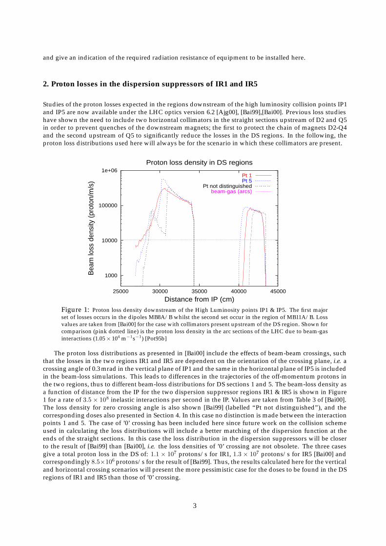
Figure 1: Proton loss density downstream of the High Luminosity points IP1 & IP5. The first majorset of losses occurs in the dipoles MB8A/B whilst the second set occur in the region of MB11A/B. Lossvalues are taken from [Bai00] for the case with collimators present upstream of the DS region. Shown forcomparison (pink dotted line) is the proton loss density in the arc sections of the LHC due to beam-gasinteractions (1.05× 104 m−1s−1) [Pot95b]

The proton loss distributions as presented in [Bai00] include the effects of beam-beam crossings, suchthat the losses in the two regions IR1 and IR5 are dependent on the orientation of the crossing plane, i.e. acrossing angle of 0.3 mrad in the vertical plane of IP1 and the same in the horizontal plane of IP5 is includedin the beam-loss simulations. This leads to differences in the trajectories of the off-momentum protons inthe two regions, thus to different beam-loss distributions for DS sections 1 and 5. The beam-loss density asa function of distance from the IP for the two dispersion suppressor regions IR1 & IR5 is shown in Figure1 for a rate of 3.5 × 108 inelastic interactions per second in the IP. Values are taken from Table 3 of [Bai00].The loss density for zero crossing angle is also shown [Bai99] (labelled “Pt not distinguished”), and thecorresponding doses also presented in Section 4. In this case no distinction is made between the interactionpoints 1 and 5. The case of ’0’ crossing has been included here since future work on the collision schemeused in calculating the loss distributions will include a better matching of the dispersion function at theends of the straight sections. In this case the loss distribution in the dispersion suppressors will be closerto the result of [Bai99] than [Bai00], i.e. the loss densities of ’0’ crossing are not obsolete. The three casesgive a total proton loss in the DS of: 1.1 × 107 protons/s for IR1, 1.3 × 107 protons/s for IR5 [Bai00] andcorrespondingly 8.5×106 protons/s for the result of [Bai99]. Thus, the results calculated here for the verticaland horizontal crossing scenarios will present the more pessimistic case for the doses to be found in the DSregions of IR1 and IR5 than those of ’0’ crossing.

3

For comparison the rate of beam-gas interactions is shown as the horizontal line in Figure 1. In localizedregions of the dispersion suppressors it can clearly be seen that proton loss rates are more than an orderof magnitude higher than in the standard arc sections. It is these regions of maximum loss rate which willdetermine the maximimum doses that equipment placed in the DS regions will have to survive. In theseregions the extra dose to be added due to beam-gas interactions is essentially negligible, whereas in othersections of the DS, where there are essentially no point losses, the extra dose due to beam-gas interactions ata given point will be comparable to (or even greater than) the contribution at that point arising from pointlosses upstream.

Note, the proton loss distributions presented here are based on the LHC optics version 6.2. Theselosses are dependent on the optics of the straight sections of the interaction region. The following dosedistributions remain valid as long as there are no major changes to the inner region optic layouts of IR1 orIR5.

3. FLUKA simulation of the LHC dispersion suppressor regions IR1 & IR5

In the following the hadronic cascade simulations were performed using the Monte-Carlo particle showercode FLUKA[Fas01a], [Fas01b], using as full and accurate description of the DS main dipole (MB) andquadrupole (MQ, MQTL, MQM, MQML) magnets as possible.

3.1 The geometry

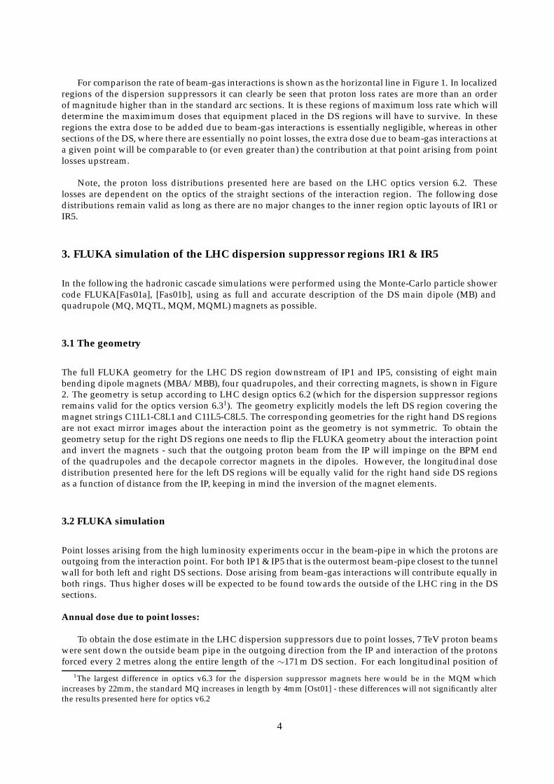
The full FLUKA geometry for the LHC DS region downstream of IP1 and IP5, consisting of eight mainbending dipole magnets (MBA/MBB), four quadrupoles, and their correcting magnets, is shown in Figure2. The geometry is setup according to LHC design optics 6.2 (which for the dispersion suppressor regionsremains valid for the optics version 6.31). The geometry explicitly models the left DS region covering themagnet strings C11L1-C8L1 and C11L5-C8L5. The corresponding geometries for the right hand DS regionsare not exact mirror images about the interaction point as the geometry is not symmetric. To obtain thegeometry setup for the right DS regions one needs to flip the FLUKA geometry about the interaction pointand invert the magnets - such that the outgoing proton beam from the IP will impinge on the BPM endof the quadrupoles and the decapole corrector magnets in the dipoles. However, the longitudinal dosedistribution presented here for the left DS regions will be equally valid for the right hand side DS regionsas a function of distance from the IP, keeping in mind the inversion of the magnet elements.

3.2 FLUKA simulation

Point losses arising from the high luminosity experiments occur in the beam-pipe in which the protons areoutgoing from the interaction point. For both IP1 & IP5 that is the outermost beam-pipe closest to the tunnelwall for both left and right DS sections. Dose arising from beam-gas interactions will contribute equally inboth rings. Thus higher doses will be expected to be found towards the outside of the LHC ring in the DSsections.

Annual dose due to point losses:

To obtain the dose estimate in the LHC dispersion suppressors due to point losses, 7 TeV proton beamswere sent down the outside beam pipe in the outgoing direction from the IP and interaction of the protonsforced every 2 metres along the entire length of the ∼171 m DS section. For each longitudinal position of

1The largest difference in optics v6.3 for the dispersion suppressor magnets here would be in the MQM whichincreases by 22mm, the standard MQ increases in length by 4mm [Ost01] - these differences will not significantly alterthe results presented here for optics v6.2

4

-10000

-8000

-6000

-4000

-2000

0

2000

4000

6000

8000

-200 -100 0 100 200 300

To interaction point (IP) ↑ 268.9 m

proton directions

↓↑MB8B

MB8A

Q8

MB9B

MB9A

Q9

MB10B

MB10A

Q10

MB11B

MB11A

missing magnet

Q11

Figure 2: FLUKA simulation of the left DS geometry for IR1 & IR5, specifically for C11L1-C8L1 andC11L5-C8L5 under LHC optics version 6.2. All dimensions are in (cm). Longitudinal dimensions relateto the FLUKA coordinate system which is centred by the quadrupole Q9. The Interaction Point IP1 orIP5 lies ∼268 m from MB8B. The directions of the 7 TeV proton beams are indicated by the single arrows.

the proton interaction point a separate simulation run is required. Energy depostion was scored in varioussized meshes covering the entire geometry: 2× 2× 50 cm3 mesh bins were used in the central regions tocover the beam-pipe and coil sections; bins of size 5× 5× 50 cm3 were used to cover the magnet yokes andcryostat regions and bins of size 20× 20× 50 cm3 were used to score dose in the air of the tunnel, tunnelwalls and floor. Details of the dose at a specific longitudinal position in the DS section are known to 50 cm(longitudinal dimension of scoring bin). The final energy deposition in each mesh bin is the total of allcontributions arising from each of the interaction point runs. This is a valid method for obtaining the totaldose since contributions arising upstream of the interaction point are orders of magnitude lower than thedose deposited downstream under the development of the hadronic and electromagnetic cascades - thereis essentially no backscattering. Due to the local nature of the proton point losses, each run in which theprotons are forced to interact at a given longitudinal position from the IP has to be weighted accordingly tothe loss density (as given in Figure 1) at that distance from the IP before summation. For a given interactionpoint, the resulting particle cascades contribute to the dose at all points downstream of the interaction point.The significance of its contribution to the total energy deposition at a position far downstream of the losspoint will be determined by its weighting, i.e. losses in the magnets where the maximum loss density occurs(MB8, Q8), will contribute a significant energy deposition in the end regions of the dispersion suppressors(missing magnet and Q11) in addition to the energy deposition resulting from losses closer to these magnets.

The total energy deposition (GeV) weighted by the loss density is then converted to Dose (1 Gy=1 J/Kg)to give the annual dose per year in each scoring bin. Due to the large proportion of neutrons produced by

5

interactions within the magnet material surrounding the beam pipes, dose estimations are sensitive to thetype of material used to score energy deposition [Huh96], i.e. dose scored in a hydrogenous material suchas polythene can be as much as twice the dose scored in an inorganic material such as aluminium or air.Thus, this simulation uses the correct material for each magnet component wherever possible to providethe most accurate dose estimation for the different sections in the magnets.

Total annual dose:

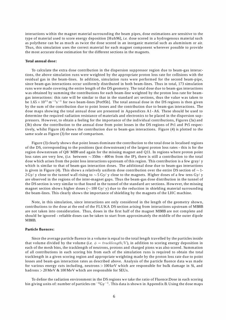
To calculate the extra dose contribution in the dispersion suppressor region due to beam-gas interac-tions, the above simulation runs were weighted by the appropriate proton loss rate for collisions with theresidual gas in the beam-lines. In addition, simulation runs were performed for the second beam-pipe,since beam-gas interactions occur uniformly distributed in both beam-lines. Thus in total, 173 simulationruns were made covering the entire length of the DS geometry. The total dose due to beam-gas interactionswas obtained by summing the contributions for each beam-line weighted by the proton loss rate for beam-gas interactions: this rate will be similar to that in the standard arc sections, thus the value was taken tobe 1.65× 1011 m−1s−1 for two beam-lines [Pot95b]. The total annual dose in the DS regions is then givenby the sum of the contribution due to point losses and the contribution due to beam-gas interactions. Thedose maps showing the total annual dose are presented in Appendices A1 - A6. These should be used todetermine the required radiation resistance of materials and electronics to be placed in the dispersion sup-pressors. However, to obtain a feeling for the importance of the individual contributions, Figures (3a) and(3b) show the contribution to the annual dose from point losses in the DS regions of Pt1 and Pt5 respec-tively, whilst Figure (4) shows the contribution due to beam-gas interactions. Figure (4) is plotted to thesame scale as Figure (3) for ease of comparison.

Figure (3) clearly shows that point losses dominate the contribution to the total dose in localised regionsof the DS, corresponding to the positions (just downstream) of the largest proton loss rates - this is for theregion downstream of Q8/MB9 and again for the missing magnet and Q11. In regions where proton pointloss rates are very low, (i.e. between ∼ 350m - 400 m from the IP), there is still a contribution to the totaldose which arises from the point loss interactions upstream of this region. This contribution is a few gray/ywhich is similar to that of beam-gas interaction doses. The additional dose due to beam-gas interactionsis given in Figure (4). This shows a relatively uniform dose contribution over the entire DS section of ∼ 1-2 Gy/y close to the tunnel wall rising to ∼ 5 Gy/y close to the magnets. Higher doses of a few tens Gy/yare observed in the regions of the inter-magnet gaps. Thus the beam-gas dose distribution in the tunnel ofthe DS section is very similar to that found in the tunnel of the standard arc sections. However, the missingmagnet section shows higher doses (∼ 100 Gy/y) due to the reduction in shielding material surroundingthe beam-lines. This clearly shows the importance of shielding by the magnets of the LHC machine.

Note, in this simulation, since interactions are only considered in the length of the geometry shown,contributions to the dose at the end of the FLUKA DS section arising from interactions upstream of MB8Bare not taken into consideration. Thus, doses in the first half of the magnet MB8B are not complete andshould be ignored - reliable doses can be taken to start from approximately the middle of the outer dipoleMB8B.

Particle fluences:

Since the average particle fluence in a volume is equal to the total length travelled by the particles insidethat volume divided by the volume (i.e. φ = tracklength/V ), in addition to scoring energy deposition ineach of the mesh bins, the tracklength of neutrons, protons and charged pions was also scored. Summationof all contributions in each scoring bin from each of the simulation runs is required to obtain the totaltracklength in a given scoring region and appropriate weighting made by the proton loss rate due to pointlosses and beam-gas interaction rates as described above. Analysis of the particle fluence data was madefor various energy cuts including, neutrons > 100 keV which are responsible for bulk damage in Si, andhadrons > 20 MeV & 100 MeV which are responsible for SEUs.

To define the radiation environment in the DS regions we take the ratio of Fluence:Dose in each scoringbin giving units of: number of particles cm−2Gy−1. This data is shown in Appendix B. Using the dose maps

6

-10000

-8000

-6000

-4000

-2000

0

2000

4000

6000

8000

-200 -100 0 100 200 3001.0E-01

2.2E-01

4.6E-01

1.0E+00

2.2E+00

4.6E+00

1.0E+01

2.2E+01

4.6E+01

1.0E+02

2.2E+02

4.6E+02

1.0E+03

2.2E+03

4.6E+03

1.0E+04

2.2E+04

4.6E+04

1.0E+05

2.2E+05

4.6E+05

1.0E+06

-10000

-8000

-6000

-4000

-2000

0

2000

4000

6000

8000

-200 -100 0 100 200 3001.0E-01

2.2E-01

4.6E-01

1.0E+00

2.2E+00

4.6E+00

1.0E+01

2.2E+01

4.6E+01

1.0E+02

2.2E+02

4.6E+02

1.0E+03

2.2E+03

4.6E+03

1.0E+04

2.2E+04

4.6E+04

1.0E+05

2.2E+05

4.6E+05

1.0E+06

(a) (b)Figure 3: Contribution to annual dose (Gy/y) in dispersion suppressor regions due to point losses fora) DS1 (proton loss weighting given by red solid line in Figure (1)) and b) DS5 (proton loss weightinggiven by blue dashed line in Figure (1)).

of Appendix A, absolute values for the particle fluence can easily be obtained.

3.2.1. Extra detail of the quenchdiode regions

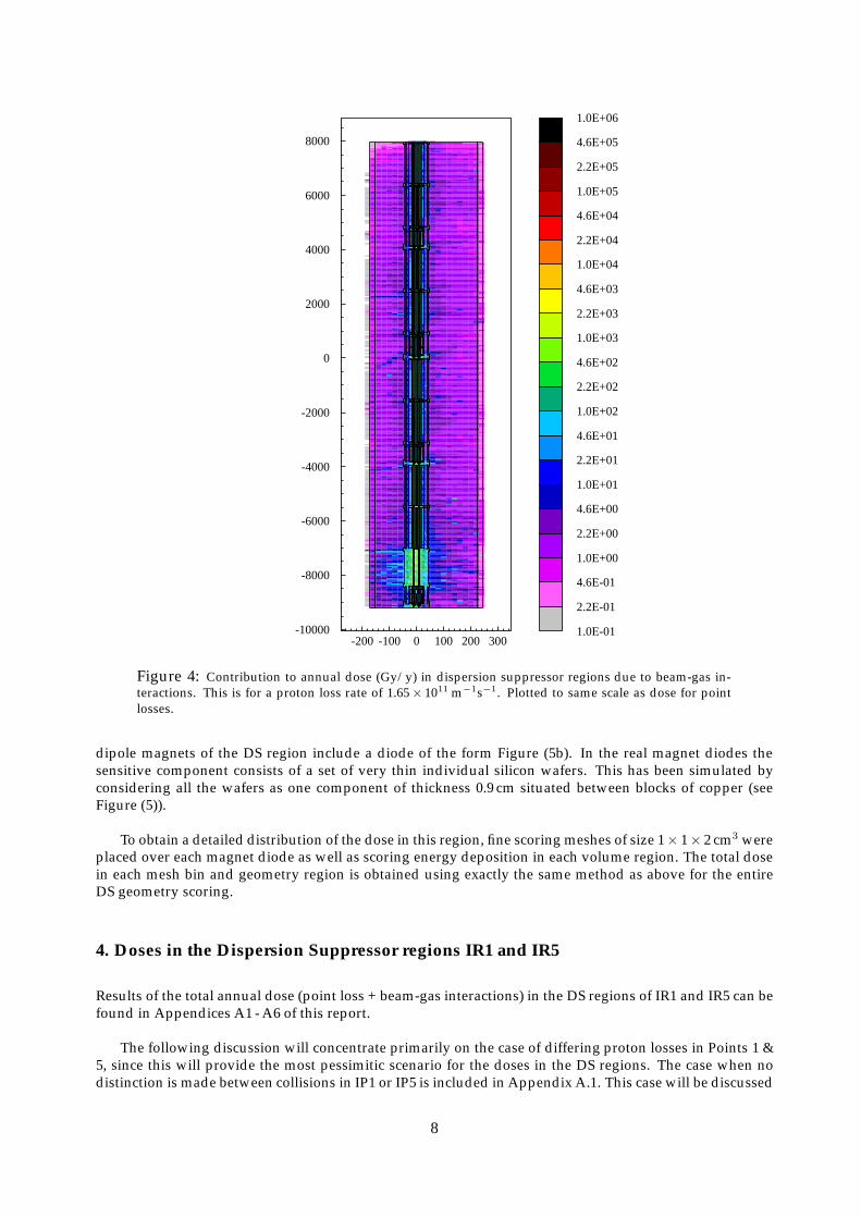
In order to determine whether expensive, high radiation tolerant quench diodes will be required in thedispersion suppressors of the LHC, the intricate design of the magnet diodes has been reproduced in asmuch detail as possible for both dipole and quadrupole diodes. This is to estimate as accurately as possiblethe dose distribution within the volume of the diode housing region and to individual components e.g thesilicon wafers. A previous study of dose to the quench diodes due to beam-gas interactions in the LHCarcs has provided preliminary estimates of the total dose to the volume within the diode housing. Thisgives a figure of 180 Gy for 10 years averaged over the whole diode region for two rings and shows anorder of magnitude gradient in the radial dimension across the diode [Ste97]. In this simulation the variouscomponents of the diode have been included separately with their respective material composition. Theexplicit geometry is shown in Figure (5a) for the quadrupole diode Q11 (note: in the dispersion suppressorsof IR1 and IR5, only Q11 contains a quench diode), and Figure (5b) for the dipole diodes. All simulated

7

-10000

-8000

-6000

-4000

-2000

0

2000

4000

6000

8000

-200 -100 0 100 200 3001.0E-01

2.2E-01

4.6E-01

1.0E+00

2.2E+00

4.6E+00

1.0E+01

2.2E+01

4.6E+01

1.0E+02

2.2E+02

4.6E+02

1.0E+03

2.2E+03

4.6E+03

1.0E+04

2.2E+04

4.6E+04

1.0E+05

2.2E+05

4.6E+05

1.0E+06

Figure 4: Contribution to annual dose (Gy/y) in dispersion suppressor regions due to beam-gas in-teractions. This is for a proton loss rate of 1.65× 1011 m−1s−1. Plotted to same scale as dose for pointlosses.

dipole magnets of the DS region include a diode of the form Figure (5b). In the real magnet diodes thesensitive component consists of a set of very thin individual silicon wafers. This has been simulated byconsidering all the wafers as one component of thickness 0.9 cm situated between blocks of copper (seeFigure (5)).

To obtain a detailed distribution of the dose in this region, fine scoring meshes of size 1× 1× 2 cm3 wereplaced over each magnet diode as well as scoring energy deposition in each volume region. The total dosein each mesh bin and geometry region is obtained using exactly the same method as above for the entireDS geometry scoring.

4. Doses in the Dispersion Suppressor regions IR1 and IR5

Results of the total annual dose (point loss + beam-gas interactions) in the DS regions of IR1 and IR5 can befound in Appendices A1 - A6 of this report.

The following discussion will concentrate primarily on the case of differing proton losses in Points 1 &5, since this will provide the most pessimitic scenario for the doses in the DS regions. The case when nodistinction is made between collisions in IP1 or IP5 is included in Appendix A.1. This case will be discussed

8

-60

-40

-20

0

20

40

60

-9120 -9110 -9100 -9090 -9080 -9070 -9060 -9050 -9040

-60

-40

-20

0

20

40

60

-7040 -7030 -7020 -7010 -7000 -6990 -6980 -6970

wafer 1 ↑ ↑wafer 2

wafer ↑

Figure 5: FLUKA simulation of the a) quadrupole and b) dipole diodes in the dispersion suppressors.Each dipole in the DS lattice includes a diode of the form (b). In the DS regions IR1 and IR5, the onlyquadrupole to have a quench diode is Q11. In the simulation the individual thin Si wafers of the diodehave been placed together to form one Si wafer of thickness 0.9 cm (2 wafers in the case of the quadrupolediode). These are indicated by the arrows above.

briefly in Section 4.1.4 since these values are not necessarily obsolete [Bai00].

Note on the scale keys of dose maps:In the following appendices, all dose maps are given to the same scale. For plots with horizontal keys, dueto space restrictions and clarity of reading it is not possible to give all division labels on the plot. The exactvalue of a given colour code can be obtained from the vertical keys of other plots in which the labelling isgiven for all divisions.

4.1. Doses in and around the DS magnets

The expected annual doses in the LHC tunnel surrounding the magnet string are given in Appendix A.1.Figures 12 - 14 show the doses radially out from the magnet string to the tunnel wall for the points 1, 5and for the case when no distinction is made between the two points (pt0) respectively. The doses expectedabove and below the magnet string are shown in Figures 16 - 18. Specific details for each cut are given withthe relevant figure. The dose maps show similar distributions for the three cases due to the similarity of thepoint loss distributions used in the weighting of the energy deposition runs. Point 5 tends to show largerextended regions of higher dose than Point 1 due to it having the higher loss density of the two.

4.1.1. Doses alongside the dispersion suppressor magnets

Plots of the dose alongside the magnet string at the height of the beam-axis are found in Figures 12 & 16 andFigures 13 & 17 for DS1 and DS5 respectively. Here the localised nature of the point loss distributions canclearly be seen. “Hot-spots” occur in the vicinity of the dipole magnets MB9A and MB9B, reaching annualdoses in excess of ∼ 200 Gy/y alongside the magnets and 100 Gy/y at the outer tunnel wall, for both Points

9

1 and 5. This “hotest” region extends the full length of MB9B for Point 5, whilst being much smaller forPoint 1. Alongside MB9B for both Points 1 & 5 typical doses are easily 100 Gy/y. Alongside dipoles MB9Adoses are a few tens of gray reaching as high as∼ 100 Gy/y (however with the indication that in the centralregions one could see a few areas reaching values of ∼ 1000 Gy/y). This higher dose region extends asfar downstream as the quadrupole Q9 where one can still find doses up to ∼ 100 Gy/y close to the magnetcryostat falling to a few tens of gray at the outer tunnel wall. These “hot-spots” are due to the fact thatthe maximum of the proton loss density for both regions occurs upstream of the dipoles MB9, hence theresulting maximum dose deposition is some metres downstream of the maximum loss point in MB8A/Q8.Other significant “hot” regions are found in the vicinity of the missing magnet and the quadrupole Q11.These are due to the second set of large proton losses occuring in this vicinity (see Figure 1) as well as thecontributions to the dose from the region of maximum proton loss upstream near Q8. Doses alongsideQ11 are a few tens to 100 Gy/y, reaching several hundreds of gray per year close to the magnet cryostat.In the magnet regions where there are essentially no point losses (MB10A, Q10 and MB11B) the total dosearising from upstream point loss contributions plus beam-gas interactions is comparable to those found inthe LHC standard arc sections. Due to the fact the dominant proton losses in the DS regions arise from pointlosses, there is no uniform dose distribution along the magnet string. This makes it difficult to determinea “typical” dose alongside a dipole, quadrupole or gap region. To give an indication of the radial dosedistribution in the LHC tunnel, cross-sectional cuts can be found in Appendix A.3 for the regions of higherdose by MB9M and Q11 for DS1 and DS5. All other positions in the tunnel of the dispersion suppressorswill see lower doses than these.

By far the hottest region in the dispersion suppressors of Points 1 and 5 is the section containing themissing magnet. Here doses within the cryostat are thousands of gray per year, falling to hundreds ofgray per year at the outer tunnel wall (with possible spots reaching a few thousands of gray per year in thespace between the cryostat and the outer tunnel wall). This is an obvious candidate for a position that couldcause problems with equipment/electronics if they have to be placed close to this spot. One possibility forreducing the dose in this region would be to fill the cryostat region with extra material.

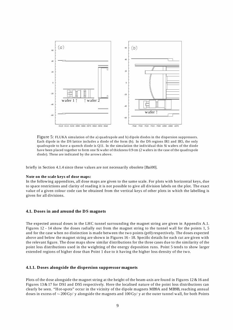
Proton point losses in the DS occur in the beam-pipe closest to the outer tunnel wall, hence we observethe maximum dose towards the outside of the ring. On the opposite side of the magnet string, (inside thering), the dose from point losses can be up to an order of magnitude lower. Doses do however still reacha few tens of gray per year opposite MB9B at the position of the tunnel wall and a few hundreds of grayper year in the vicinity of the missing magnet and Q11. To give an overview of the DS region a summary ofthe longitudinal dose distribution at the cryostat surface and at the tunnel wall for each magnet is given inFigure (6) for IR1 and Figure (7) for IR5.

4.1.2. Doses under the dispersion suppressor magnets

Maps showing the dose due to point losses under the magnet string in the DS regions of Points 1 and 5 canbe seen in Figures (16) and (17) respectively. These are averaged over a 60 cm slice about the central pointbetween the beam-pipes (40 cm slice in the central region) as shown in Figure (11). In general, the dosesunder the magnet string are not so high as those directly alongside the outside of the magnet string at thelevel of the beam-axis. For both DS regions, doses will be less than ∼ 100 Gy/y, except under Q11 and theempty cryostat region. Here doses can reach ∼1000 Gy/y. To give a summary of the expected dose underthe DS magnet string, the longitudinal dose distribution averaged over a height of 30 cm lying between thecryostat and the floor surface (of the doses presented in Figures (16) and (17)), are shown in Figures (8a)and (8b) respectively for Points 1 and 5.

4.1.3. Doses in the tunnel floor of the dispersion suppressors

In the vicinity of the regions of highest proton loss we note that higher doses will also be observed inthe concrete floor of the tunnel. Maps showing the dose distribution in the tunnel floor can be found in

10

Appendix A.2. For DS1, in the vicinity of MB9B doses of the order ∼ 50 Gy/y are seen, with higher dosesof ∼ 100 Gy/y observed for the same position in DS5. Higher doses are seen in the vicinity of the missingmagnet and Q11, reaching values possibly as high as ∼ 1000 Gy/y in both DS regions. This could be ofconcern for any radiation sensitive equipment that will be placed on the tunnel floor.

4.1.4. Dose in dispersion suppressors for case with no distinction made between IR1 and IR5

Results for the case where no distinction is made between Points 1 and 5 (Appendix A.1: Figures 14 & 18)show similar distributions to those discussed above, although hot-spot regions tend to have lower dosemaxima and are less extended than those when the two Points are considered separately. Due to furtherwork to be performed regarding the absolute loss distributions in the dispersion suppressors, these resultsare not obsolete [Bai00] and are included here for completeness.

4.2. Maximum dose in the inner regions of the dispersion suppressors

Maximum doses are observed radially outwards in the beam-axis plane. Due to the large dose gradientabout the beam-axis (i.e. doses above/below the beam-axis are much lower than along the beam-axis),to obtain an estimate of the maximum doses to components that will be situated around the beam-axis,Figures (23) and (26) in Appendix A.4 show the annual dose averaged over a 4 cm slice2 about the beam-axis for the inner regions of the magnets for the length of the dispersion suppressor regions of Points 1 and5 respectively. The dose distribution along the beam-pipes in the DS is not constant due to the non-uniformlongitudinal proton loss distribution. The maximum dose reaches a value of at least 105Gy/y along theouter beam-pipe of both MB9 dipole magnets. Typical doses along the beam pipes in other sections ofthe dispersion suppressors are of the order 103-104 Gy/y, which are similar to the levels found along thebeam-pipes in the standard arc sections.

4.2.1. Dose along beam-pipe in MB9 section - on beam-axis

The maximum dose occurs a few metres downstream of the maximum proton loss points, thus maximumdoses are observed along the beam-pipe of the dipole magnets MB9A and MB9B. The maximum doseaveraged over 4 cm about the beam-axis for the inner regions of magnets MB9A/B is shown in AppendixA.4 (Figures 24 and 27) and a selection of cross-sectional cuts through the outer beam pipe of these magnetsin Figures 25 and 28. In the inner magnet coils, maximum doses are observed in the plane of the beam-axisand to the side in which the dipole magnetic field is biasing the particles (towards the inside of the ring).Doses as high as ∼2.2× 105 Gy/y are found in the beam-screens/pipes and inner coils of DS1 and maximaapproximately a factor 2 higher in DS5 (∼5× 105 Gy/y). There is at least an order of magnitude differencein the annual dose between the top:middle and bottom:middle of the coils. For components which will beinstalled between magnets and close to the beam-pipes, these should be able to withstand annual doses of∼105 Gy/y to ensure survival at all positions in the dispersion suppressors.

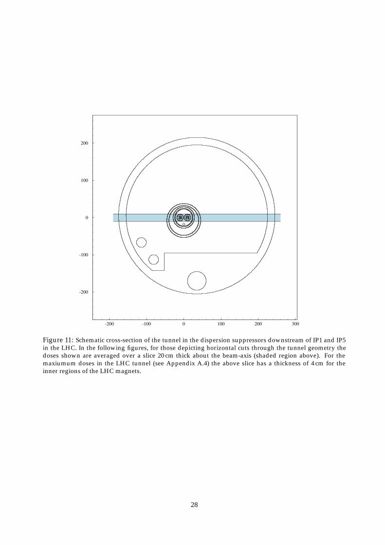
2This is for the same cut as shown in Figure (11), but the shaded region covers a slice of 4 cm about the axis for theinner magnet regions, not 20 cm.

11

Figure 6: Doses alongside the magnets of the dispersion suppressors of PT1 for a radial position atthe surface of the cryostat (black line) and at the tunnel wall (pink line). The upper plot shows thelongitudinal dose distribution at the height of the beam-axis averaged over a 20 cm slice (see Fig. 11)outside of the LHC ring. The lower plot shows the longitudinal distribution for the same radial positionsbut for the inside of the LHC ring. To guide the eye, the horizontal dotted lines indicate the 100 Gy/ymark and the 1000 Gy/y mark. The schematic under the plot indicates the position of the individualmagnets, delimited by their virtual interconnection planes.

12

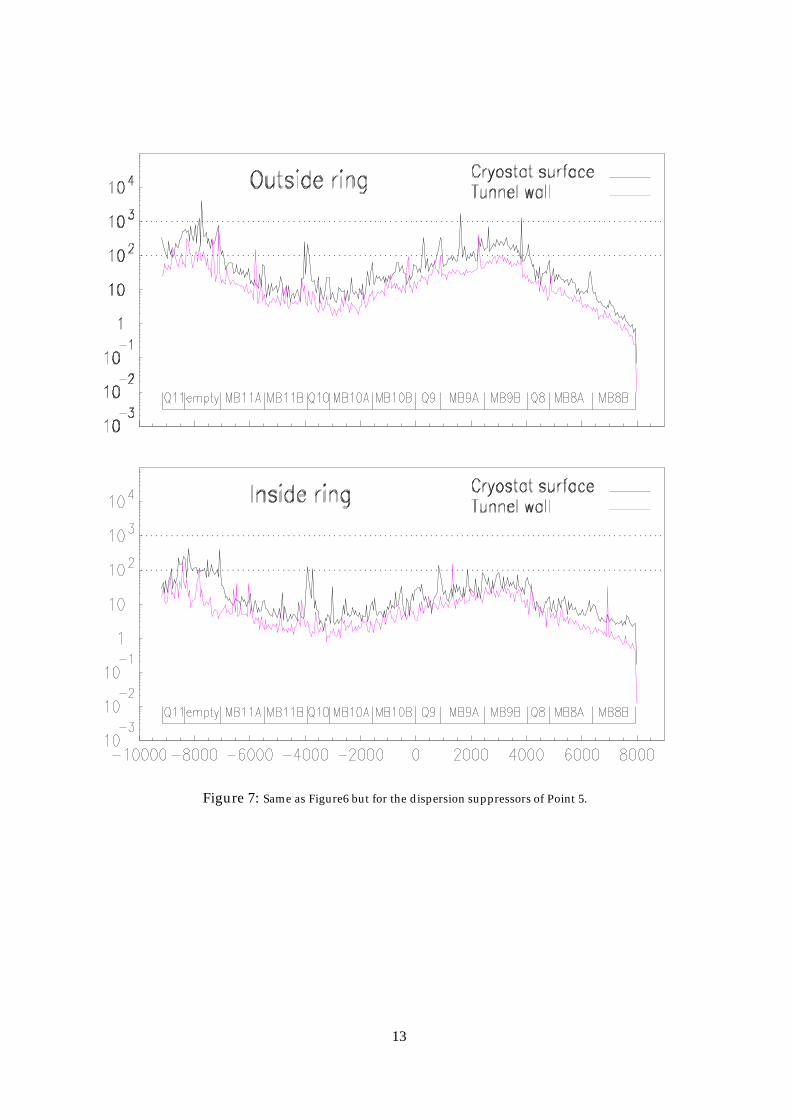
Figure 7: Same as Figure6 but for the dispersion suppressors of Point 5.

13

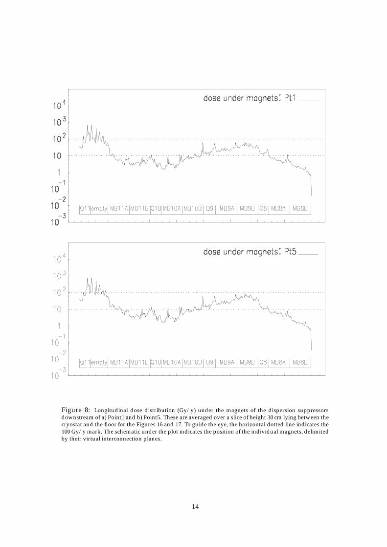
Figure 8: Longitudinal dose distribution (Gy/y) under the magnets of the dispersion suppressorsdownstream of a) Point1 and b) Point5. These are averaged over a slice of height 30 cm lying between thecryostat and the floor for the Figures 16 and 17. To guide the eye, the horizontal dotted line indicates the100 Gy/y mark. The schematic under the plot indicates the position of the individual magnets, delimitedby their virtual interconnection planes.

14

4.2.2. Dose to BPMs of dispersion suppressors: Q8-Q11

Annual dose to the Beam Position Monitors of the dispersion suppressors is shown for each quadrupolemagnet in Appendix A.5 (Figures 29 (a)-(d) and 30 (a)-(d) for DS1 and DS5 respectively). These plots areaveraged over a total height 12 cm above and below the beam-axis to cover the extent of the BPM. Maximumdoses are similar for the dispersion suppressors of Points 1 and 5. The BPMs belonging to Q10 tend to havelower maximum doses along the outer beam pipe than for the other quadrupoles. This is due to the lowproton point loss rate at this point. Maximum doses close to the beam-pipe for Q8, Q9 and Q11 are of theorder several 104 Gy/y, whereas for Q10 this value falls to several 103 Gy/y. The dose to the BPM is lowerfor the second beam-line since the dose at this postion does not receive such a large contribution from thepoint loss interactions, as for the outgoing beam-line. The lower dose region observed for the BPM of Q11for the second beam-line (for both DS1 & DS5) is an artifact of the Monte-Carlo simulation. This is due toits position at the end of the geometry - since protons are sent down the beam-line starting at the end ofthe geometry, contributions to the dose at this point arising from interactions upstream in the arcs are notincluded. Realistic dose values for the second beam-line of Q11 should be similar to those shown in plots(a)-(c) for the other BPMs.

4.3. Dose to the quenchdiodes in the dispersion suppressor regions

Table 1: Summary of dose to the quench diodes in the dispersion suppressors of IR1 and IR5. Valuesfor the dose averaged over the entire diode housing region as well as the dose specifically to the Si inthe diodes are given for each magnet. In the DS of IR1 and IR5 the only quadrupole to have a diodeis Q11.

Average dose over entire Doses to Si in diode regionlattice element diode region Gy/y lattice element Gy/y

Pt 1 Pt 5 Beam-gas Pt 1 Pt 5 Beam-gasQ11 116.1 127.8 12.9 Q11 Si wafer 1 100.3 134.3 13.2- - - - Q11 Si wafer 2 57.7 63.3 11.8MB11A 32.9 44.3 16.8 MB11A 8.3 10.7 1.5MB11B 8.3 9.4 6.5 MB11B 1.8 2.3 1.7MB10A 6.3 6.4 5.0 MB10A 1.2 1.2 0.8MB10B 10.8 13.3 5.4 MB10B 1.8 1.8 1.8MB9A 67.6 75.4 5.3 MB9A 15.8 16.7 1.2MB9B 400.8 497.5 15.7 MB9B 38.3 47.2 1.9MB8A 25.0 20.0 3.6 MB8A 10.8 9.9 1.3MB8B 9.2 7.5 5.3 MB8B 5.9 4.6 2.6

Maps of dose due to point losses in the quench diodes for each magnet element are given in AppendixA.6. Figures (31) - (40) show the doses in the dispersion suppressors for both IR1 and IR5. Very littledifference is seen between the two regions. To summarise the doses to the magnet diodes, Table 1 shows a)the average annual dose to the entire diode region (i.e. averaged over the volume within the diode housingand b) the annual dose to the Si wafers for dispersion suppressors IR1, IR5. The values averaged over thevolume of the diode housing for each magnet provide an order of magnitude estimate of the annual doseto individual diodes in the DS regions. The 3rd column of each section (labelled ’Beam-gas’) shows thecontribution to the dose from beam-gas interactions. This provides an indication of the dose to the quenchdiodes in the standard arc sections. The results of dose to the Si wafers were obtained from the total energydeposition within the Si region of the simulation. These values are not reliant on the mesh scoring in whichbins could contain contributions from other elements within the diode housing; thus this should provide agood estimate of the dose to the sensitive silicon of the diodes and accounts for the large differences seenbetween the two sets of values.

15

In general the annual dose to the sensitive silicon components of the quench diodes is very low withexceptions to the diodes of quadrupole Q11 and possibly MB9B. For 10 years of LHC running total dosesshould not exceed 1 kGy (Si diode of Q11 in Pt5 excepted). The larger dose values seen over the entire diodevolume are due to the large dose gradient across the diode volume - there is a strong top:bottom gradientof at least an order of magnitude difference in the doses, with an increase in dose seen towards the frontend intermagnet-gap region.

Corresponding values for the neutron fluences above various energy cuts at the position of the quenchdiodes are given in Table 2 in Section 6.2.

5. Annual dose in the dispersion suppressors of Points 3 & 7

To date no calculation of dose values exists for the dispersion suppressor regions of the cleaning sectionsIR3 (momentum cleaning) and IR7 (betatron cleaning). This simulation is made difficult in that we do nothave full knowledge of the point loss distribution for these regions, which is essential if we are to scale anyMonte Carlo simulation results of dose normalised for one interacting proton per metre to give absolutevalues of annual dose.

Obtaining proton loss distributions for the DS sections of the scraping regions of the LHC ring is moredifficult than for the DS regions downstream of the high luminosity interaction points, due to the nature ofthe collision points. Calculation of proton losses downstream of IR3 and IR7 is made more difficult sincethe source points are distributed in the collimator jaws of the insertion sections, compared to the uniquesource point for the experimental interaction regions. This leads to quite large statistical uncertainties inthe loss distributions in the DS regions of IR3 and IR7. Another problem is that the point loss distributionsdownstream of the scraping regions are dependent on the layout of the collimators in these sections. Todate, the design of these is not fully fixed making absolute predictions for the proton loss distributions inthe DS regions of IR3 and IR7 impossible.

1000

10000

26002650270027502800285029002950300030503100

Bea

m lo

ss d

ensi

ty (m

-1s-1

)

Distance to IP8 (m)

Proton loss density in DS regions of IR3 and IR7

normalised to primary flux of n=3x109 p/sin the collimation insertion

B8B

QD8

B9B

B11B

MB

MB

proton loss distribution beam-gas (lifetime 250hr)beam-gas (lifetime 85hr)

Figure 9: Proton loss density in the dispersion suppressors of IR3 and IR7 as given in [Jea01a]. Thelongitudinal coordinate has an arbitrary origin at IP8.

However, an indication of the expected proton loss distributions in these regions does exist. This allowsus to draw some general conclusions regarding the expected annual dose distributions in the DS regions ofIR3 and IR7. Estimation of the expected proton loss rates downstream of the scraping sections of the LHCcan be found in [Jea01a]. This data is reproduced in Figure (9), which is normalised to a primary flux of

16

3× 109 protons/s in the collimation insertion. [Jea01a] reports that similar integrated loss rates are com-puted for the betatron and momentum collimation insertions which allow us to use the same differentialproton loss distribution for both IR3 & IR7. This data is plotted as a function of distance from the LHCpoint IP8, which is taken to be an arbitrary origin. The difference in the losses in IR3 and IR7 will be theabsolute normalisation of the results, which is not known at present. This estimation of the losses is basedon LHC optics verion 5.0. Proton loss distributions are dependent on the layout of the scraper insertionregions, however, no significant changes were seen beyond the extent of the cleaning regions in the longstraight sections for higher optics versions[Jea01b]. Therefore this data can be used to give an estimate oflosses in the DS sections downstream of the scraper regions for the current LHC version.

Even though proton losses for the scraper regions have a different origin than those for the collisionregions, the off-momentum proton losses in the dispersion suppressors are very similar. This is shownin Figure (9) where we see a very similar proton loss distribution downstream of the scraper regions, asthat seen downstream of the high luminosity interaction points (see Figure (1)) i.e. losses occur in thesame magnets. We note that the point loss magnitude is much less than that in IR1 & IR5. The maximumpoint loss densities reach ∼ 3 times higher than the beam-gas loss rate in the standard arc and dispersionsuppressors as given for the LHC Design Machine (blue dotted line in Figure (9)). In fact, the magnitudeof point losses beyond MB9 in the DS and arc sections of IR3 and IR7 is lower than that of the beam-gas interaction rate. Thus for these regions, beam-gas interactions can be considered to be the dominantcontribution to the total dose; point losses are essentially negligible.

This implies that we expect to see similar point loss dose distributions in the dispersion suppressors ofthe scraper regions as those shown in Figure (3), but with a magnitude similar to that of the beam-gas dose.The dominant contribution to the annual dose from beam-gas interactions will have a similar distributionto that shown in Figure (4). It is important to remember that the exact normalisation is not known for these losses.Thus the contribution from point losses could be significantly higher than discussed here if a large normalisationfactor is found to be required at a later date. If so, it should be possible to scale the dose distributions aspresented in Figure (3) for IR1 & IR5 to obtain an estimate of the dose in the scraper region dispersionsuppressors, as long as the loss distribution does not significantly alter. Similarly plots of dose due tobeam-gas contributions can be scaled if necessary. In the opinion of the author, in the light of the presentinformation given by the expected point loss rates in Figure (9), further explicit Monte-Carlo simulation ofthe dispersion suppressor regions of IR3 and IR7, which would take many months of computing time, isnot warrented.

6. Radiation environment in the DS regions 1 & 5

Electronics equipment and machine components placed in the LHC tunnel will also be susceptible to thehigh energy particles found around the machine. To enable estimation of possible SEE effects, it is necessaryto know the radiation environment in which the equipment will be placed. Thus, this section presentsvalues for the fluence : dose ratios to be expected in DS1 and DS5; the maps and full information of whichcan be found in Appendix B. Using these ratio maps in combination with the relevant dose maps givenin Appendix A, values for the total annual particle fluences at a position in the LHC tunnel are readilyobtained.

6.1. Fluence:dose ratios in the dispersion suppressors DS1 & DS5

Maps of the ratio particle fluence : dose are shown in Appendix B for neutrons, protons, charged pionsand total summed hadrons above five specific energy cuts: 100 keV, 1 MeV, 20 MeV, 50 MeV and 100 MeV.Neutrons above 100 keV are responsible for causing bulk damage in Si and the higher energy hadrons areresponsible for causing Single Event Upsets (SEUs).

It is found that the radiation environment, characterised by the ratio R=fluence/dose, for the machinesection in DS1 and DS5 is the same, with variations of only a few percent seen between the two data sets. A

17

larger variation is observed for protons close to the cryostat on the outside of the LHC ring such that valuesfor the proton ratio above all energy cuts in DS5 are between 2-4 times larger than those of DS1. This will bedue to the difference in the proton loss distributions of the two sections, as the losses occur in the outgoingbeam-line close to the outside of the LHC ring. However, since the ratio maps are plotted with each decadesplit into 3 colour grades, this variation is indistinguishable between maps for DS1 or DS5, thus, only oneset of ratio maps is given. The results plotted in this report specifically use data for DS1, but are equallyvalid for both DS1 and DS5.

The radiation environment in the dispersion suppressors is not completely uniform. To give an overview,Appendix B.1. shows the longitudinal ratio distribution above and below the dispersion suppressor mag-net string for neutrons and hadrons for all energy cuts (Figures (41) and (44)), as well as the individualproton and charged pion contributions above the energy cuts 100 keV and 100 MeV (Figures (42) and (43)).Very little drop is seen in the proton and charged pion distributions between these energy cuts.

It is observed that the environment between MB11A and MB8B is the same as that for the LHC arcsections (see fluence : dose maps in [Fyn01a]). Here we observe essentially uniform ratios in the vicinity ofdipole magnets, quadrupoles and intermagnet gaps, allowing us to average over these regions to obtaina characteristic value of R alongside a dipole (n > 100 keV: ∼5×1010 cm−2, h > 100 MeV: ∼2×109 cm−2),quadrupole (n > 100 keV: ∼5×1010 cm−2, h > 100 MeV: ∼2×109 cm−2) and intermagnet gap ( n > 100 keV:∼3×1010 cm−2, h > 100 MeV: ∼1×109 cm−2) respectively. It should be noted that the ratios found in thevicinity of the missing magnet and Q11 are lower than these values. We expect∼3×109 cm−2 and∼1×1010

cm−2 for neutrons > 100 keV, with these values falling to ∼2×108 cm−2 and ∼4×108 cm−2 for hadrons> 100 MeV in the region of the missing magnet and Q11 respectively.

The distributions above/below the magnet string are very similar to those found in the beam-axis plane,as the ratio is found to be reasonably radially symetric about the machine. To give an indication of thevariation in the ratio in the LHC tunnel, Appendix B.2. shows cross sectional cuts through the tunnel forthe individual magnet components: Q11, the missing magnet, a typical dipole, quadrupole and intermagnetgap (Figures (45) - (54)), for all neutron and hadron energy cuts. These plots are obtained by averaging overthe length of the individual magnets and for the case of a “typical” magnet element by averaging furtherover the individual magnet component values, e.g. the value for a dipole is obtained by averaging over theaveraged value obtained for MB11A - MB8B. The data plotted for Q11 and the missing magnet is obtainedby averaging over the data along the length of the relevant section. Generally, variations of a ∼ few tens %are observed in performing this averaging - however, larger variations are seen when averaging over theregion of the missing magnet in which a much less uniform ratio distribution is observed. Reasonableradial symmetry is observed in the tunnel alongside magnet components, with slightly lower ratios seentowards the outside of the tunnel in the beam-axis plane for the low energy neutrons. Larger deviationsfrom uniformity are seen in the vicinity of the missing magnet where the ratio increases by approximatelyan order of magnitude between the surface of the cryostat and the tunnel wall.

To give a quantitative overview of the variation in the fluence : dose ratios found in the LHC dispersionsuppressors, Appendix B.3. provides tables of the ratio at specific positions in the LHC tunnel: specificallyfor positions alongside the cryostat, both inside and outside the LHC ring, at the tunnel wall inside andoutside the ring, under the magnet string and for 3 heights above the magnet. These values should be usedwith the corresponding dose at these positions in DS1 and DS5 to give the required annual particle fluence.Full data is given for neutrons, hadrons and the individual proton and charged pion contributions for eachenergy cut (Figures (55) - (59)). To give an idea of the statistical uncertainity on these values from averagingover the data along the length of a magnet component / over dipole magnets etc., the column, ±%, givesthe standard error on the mean in taking the average, and the column, sd %, keeps track of the standarddeviation of the values averaged - specifically the largest value between the standard deviation obtainedin averaging over the magnet component data sets, or the combined error of the standard deviations onthe ’raw’ data being averaged over. It can be seen that the data alongside dipole/quadrupole magnets isessentially uniform with small deviations of a few tens %. The largest errors are obtained in averaging overthe data to give a “characteristic” value for the missing magnet and gap sections of the machine (up to∼ 70%).

18

Figure 10: Ratios of fluence:dose as a function of the particle energy cut. Summary curves are shownfor neutrons, protons, charged pions and total summed hadrons above a given energy cut. The individualplots show the radiation environment in the vicinity of Q11, the missing magnet, a dipole, a quadrupole(not Q11) and the intermagnet gap regions for the dispersion suppressors of DS1 and DS5. Values aretaken from the averaged data in Figures (55) - (59).

19

A summary of the radiation environment for each of the magnet components is shown in Figure (10),plotted as a function of the particle energy cut. These can be used to obtain information on particle fluencesin the LHC tunnel for any arbitrary particle energy cut. In order to obtain a representative value for the ratioin the tunnel at the position of a given magnet component, the average of all data has been performed. Thequantitative values for producing these summary plots are given in the “average ratio” rows of Figures (55)- (59). It is useful to note that, the ratio values in the region of the missing magnet are representative of anyposition in the LHC machine in which one finds the bare beamline and not just the dispersion suppressors.Similarly, the values for a “typical” dipole, quadrupole and intermagnet gap are representative of thesecomponents placed elesewhere in the machine e.g LHC arc sections.

6.2. Neutron fluences at the position of the quench diodes

To estimate whether the observed particle fluences in the vicinity of the dispersion suppressor magnets willcause problems for the sensitive quench diodes, Table 2 shows the annual neutron fluence (neutrons / cm2)for each of the quench diodes in both dispersion suppressor sections. Values are given for the usual en-ergy cuts where neutrons > 100 keV are responsible for causing bulk damage in Si, and the higher energyneutrons are a source of SEEs.

It is noted that the highest neutron fluences are found at the same position as the regions of highestdose in the dispersion suppressor sections i.e. at the positions of highest proton point loss. Thus fluences of∼2-4× 1012 neutrons > 100 keV / cm2 can be expected at the positions of the quench diodes in MB9A andMB9B. All other diodes will see lower neutron fluences. Values are similar for the diodes in DS1 & DS5,especially in sections of the dispersion suppressors which see a radiation environment similar to that ofthe LHC arcs (MB11B-MB10B). At the positions of maximum proton point loss, DS5 will see slightly higherneutron fluences than the same position in DS1.

7. Summary

In this study we have performed a detailed Monte-Carlo simulation of the dispersion suppressor sectionsof LHC points 1 and 5, to determine the expected total annual dose and fluence : dose ratios from bothpoint losses (the dominant factor) and beam-gas interactions. Individual dose and fluence : dose ratio mapsfor various cuts through the dispersion suppressor geometry are given in Appendix A and Appendix Brespectively.

The plots presented here are shown as the average over a number of scoring layers, and summary plotsare obtained by taking a further average over a number of different components, e.g dipole magnets to givea “typical” value in the vicinity of a dispersion suppressor dipole. This averaging is the dominant cause ofuncertainty in the results presented here, depending on the uniformity of the dose or ratio data. It is foundthat the largest uncertainties arise when considering the intermagnet gap, or missing magnet sections dueto the more non-uniform distributions in these areas. Generally, uncertainites of a few tens percent areobtained in averaging over data in the vicinity of magnet elements, which can increase up to a factor 2 inthe gap/missing magnet regions.

Doses in the tunnel and magnets of the dispersion suppressors:

The expected total annual dose distributions from point losses in the dispersion suppressors of Points 1and 5 are very similar. The DS magnets downstream of Point 5 will however see slightly higher doses andextended hotter regions than Point 1 since the loss density downstream of Point 5 is the larger. The dosestudy presented here remains valid as long as the proton loss distributions for the DS regions remain validi.e. if the optics in the inner regions of IR1 or IR5 change, then the loss distributions downstream will alsochange.

20

Table 2: Neutron fluences above various energy cuts, at the postion of the quench diodes inthe dispersion suppressors of IR1 and IR5. Values are the averaged annual fluence over theentire diode housing volume.

Diode Annual Neutron Fluence > Ecut (cm−2.yr−1)Dispsersion Suppressor DS1100 keV 1 MeV 20 MeV 50 MeV 100 MeV

Q11 2.9× 1011 1.4× 1011 4.9× 1010 3.5× 1010 2.3× 1010

MB11A 6.5× 1011 2.1× 1011 5.7× 1010 3.8× 1010 2.2× 1010

MB11B 2.6× 1011 6.4× 1010 1.6× 1010 1.1× 1010 7.3× 109

MB10A 1.6× 1011 4.5× 1010 1.1× 1010 7.8× 109 4.5× 109

MB10B 3.2× 1011 8.7× 1010 2.3× 1010 1.7× 1010 9.2× 109

MB9A 1.9× 1012 5.3× 1011 1.3× 1011 9.1× 1010 5.4× 1010

MB9B 2.9× 1012 7.7× 1011 1.8× 1011 1.2× 1011 6.5× 1010

MB8A 1.0× 1012 3.0× 1011 7.8× 1010 5.1× 1010 2.9× 1010

MB8B 3.1× 1011 8.2× 1010 2.0× 1010 1.3× 1010 7.6× 109

Dispsersion Suppressor DS5100 keV 1 MeV 20 MeV 50 MeV 100 MeV

Q11 3.0× 1011 1.5× 1011 5.2× 1010 3.7× 1010 2.4× 1010

MB11A 9.0× 1011 2.9× 1011 7.7× 1010 5.2× 1010 3.0× 1010

MB11B 2.8× 1011 6.9× 1010 1.6× 1010 1.2× 1010 7.5× 109

MB10A 1.7× 1011 4.7× 1010 1.1× 1010 8.2× 109 4.8× 109

MB10B 3.8× 1011 1.1× 1011 3.0× 1010 2.2× 1010 1.2× 1010

MB9A 2.0× 1012 5.8× 1011 1.5× 1011 1.0× 1011 5.9× 1010

MB9B 3.8× 1012 9.8× 1011 2.3× 1011 1.6× 1011 8.4× 1010

MB8A 6.6× 1011 1.9× 1011 4.9× 1010 3.2× 1010 1.8× 1010

MB8B 2.4× 1011 6.3× 1010 1.5× 1010 1.0× 1010 5.9× 109

In general if equipment to be installed in the dispersion suppressor regions of Points 1 and 5 is ableto withstand doses of a few hundred gray per year, i.e. minimum of 103 Gy for 10 years of LHC runningthen it should be able to survive. However, it is likely that some very localized regions in the dispersionsuppressors will see even higher doses - possibly reaching thousands of gray per year which will mostprobably cause a problem for components situated at these points if they are only radiation hard to a fewhundred Gy/y. For equipment to be placed under the magnet string a limit of 102 Gy/y should ensure thatequipment will survive in all locations under the magnet string except under the empty cryostat region -here a limit of at least 103 Gy/y will be required. On a more local basis, considering the distribution of dosealong the DS magnets then the “high” dose areas are limited to a couple of dipoles, the missing magnet andQ11 regions. Other regions, alongside the magnets MB11A-MB10B will see annual doses �100 Gy/y, i.e.regions with comparable doses to the LHC standard arc sections will be found in the DS sections. A sum-mary of the required dose levels equipment will need to be able to survive is given for the different magnetelements in the DS regions in Table 3. These are explicitly for the left dispersion suppressor section; toobtain the required resistance of equipment in the vicinity of the individual magnets in the right dispersionsuppressors, the magnet labels A and B should be interchanged. The localization of the hot-spots and thenon-symmetric nature of the dose distribution shows that the positioning of equipment/electronics in theDS regions will be very important. Equipment to be positioned on the outside of the LHC ring will receivehigher annual doses than that situated inside the ring. This is because point losses occur in the outgoingproton direction from the interaction point which for both Points 1 and 5 is in the beam-pipe closest to theouter tunnel wall.

The highest doses in the DS section are found in the vicinity of the missing magnet. Here the onlymaterial surrounding the beam-pipes in which the radiation can interact is the cryostat. This region could

21

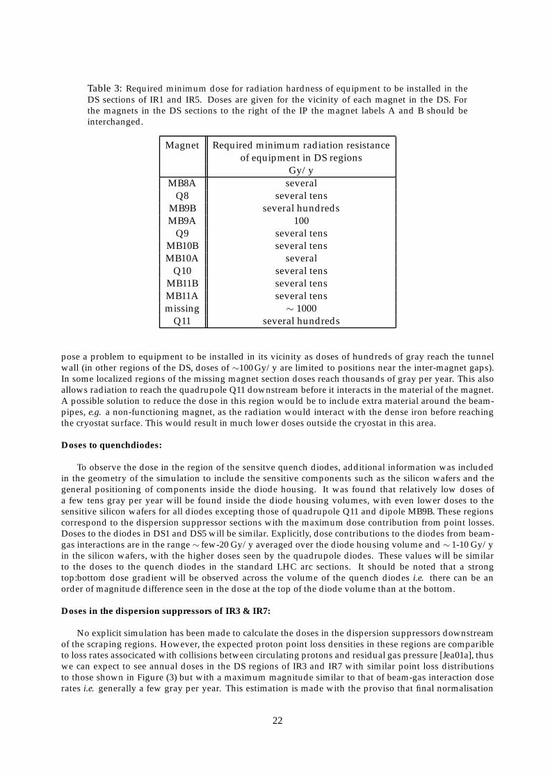
Table 3: Required minimum dose for radiation hardness of equipment to be installed in theDS sections of IR1 and IR5. Doses are given for the vicinity of each magnet in the DS. Forthe magnets in the DS sections to the right of the IP the magnet labels A and B should beinterchanged.

Magnet Required minimum radiation resistanceof equipment in DS regions

Gy/yMB8A several

Q8 several tensMB9B several hundredsMB9A 100

Q9 several tensMB10B several tensMB10A several

Q10 several tensMB11B several tensMB11A several tensmissing ∼ 1000

Q11 several hundreds

pose a problem to equipment to be installed in its vicinity as doses of hundreds of gray reach the tunnelwall (in other regions of the DS, doses of ∼100 Gy/y are limited to positions near the inter-magnet gaps).In some localized regions of the missing magnet section doses reach thousands of gray per year. This alsoallows radiation to reach the quadrupole Q11 downstream before it interacts in the material of the magnet.A possible solution to reduce the dose in this region would be to include extra material around the beam-pipes, e.g. a non-functioning magnet, as the radiation would interact with the dense iron before reachingthe cryostat surface. This would result in much lower doses outside the cryostat in this area.

Doses to quenchdiodes:

To observe the dose in the region of the sensitve quench diodes, additional information was includedin the geometry of the simulation to include the sensitive components such as the silicon wafers and thegeneral positioning of components inside the diode housing. It was found that relatively low doses ofa few tens gray per year will be found inside the diode housing volumes, with even lower doses to thesensitive silicon wafers for all diodes excepting those of quadrupole Q11 and dipole MB9B. These regionscorrespond to the dispersion suppressor sections with the maximum dose contribution from point losses.Doses to the diodes in DS1 and DS5 will be similar. Explicitly, dose contributions to the diodes from beam-gas interactions are in the range∼ few-20 Gy/y averaged over the diode housing volume and∼ 1-10 Gy/yin the silicon wafers, with the higher doses seen by the quadrupole diodes. These values will be similarto the doses to the quench diodes in the standard LHC arc sections. It should be noted that a strongtop:bottom dose gradient will be observed across the volume of the quench diodes i.e. there can be anorder of magnitude difference seen in the dose at the top of the diode volume than at the bottom.

Doses in the dispersion suppressors of IR3 & IR7:

No explicit simulation has been made to calculate the doses in the dispersion suppressors downstreamof the scraping regions. However, the expected proton point loss densities in these regions are comparibleto loss rates associcated with collisions between circulating protons and residual gas pressure [Jea01a], thuswe can expect to see annual doses in the DS regions of IR3 and IR7 with similar point loss distributionsto those shown in Figure (3) but with a maximum magnitude similar to that of beam-gas interaction doserates i.e. generally a few gray per year. This estimation is made with the proviso that final normalisation

22

of the proton point losses in these regions may differ, such that these regions may pose more of a radiationproblem than the currently available loss data indicates.

Particle fluences in the dispersion suppressors:

In order that estimation can be made of Single Event Effect problems occuring with the equipmentplaced in the tunnel in the vicinity of the dispersion suppressors, it is necessary to have an idea of theradiation environment it will be placed in. Details of the radiation environments of DS1 and DS5 are givenin Appendix B of this report in the form of fluence : dose maps. The high energy particle fluences havebeen presented in this way since it is found that the ratio R = fluence/dose is the same for both dispersionsuppressors. Absolute magnitudes of neutron, proton, charged pion, as well as the total summed hadron,fluences can readily be obtained by combining the ratio data with the dose data presented in Appendix Aat a given position in the LHC tunnel.

Typical ratio values of fluence : dose can be obtained for standard dipole and quadrupole magnets: avalue of ∼ 5× 1010cm−2Gy−1 is found for neutron fluences > 100 keV, which falls to ∼ 2× 109 cm−2Gy−1

for hadrons > 100 MeV. These values are also representative of the fluence : dose ratio seen at other posti-tions in the LHC machine, such as the standard arc sections [Fyn01a]. Ratios corresponding to the missingmagnet section and quadrupole Q11 of the dispersion suppressor regions are lower than these values by upto an order of magnitude. Detailed values of the fluence : dose ratios are provided in Figures (55) - (59) forfive different energy cuts, for each particle species and for differing positions in the LHC tunnel. A sum-mary of the data showing the ratio as a function of the particle energy cut is given in Figure (10). This canbe used to determine absolute particle fluences in the dispersion suprressors for any arbitrary energy cut,which when combined with further information on nuclear interaction probabilities [Huh00] can provideestimates of SEU rates expected for the electronics placed in the LHC tunnel.

References

[Ajg00] I. Ajguirei, I. Baichev and J. B. Jeanneret, Beam losses far downstream of the high luminosity interactionpoints of LHC, LHC Project Report 398.

[Bai99] I. Baichev, J. B. Jeanneret and G. R. Stevenson, Beam losses far downstream of the high luminosity inter-action points of LHC - intermediate results, LHC Project Note 208.

[Bai00] I. Baichev, Proton losses in the dispersion suppressors of IR1 and IR5 of LHC, LHC Project Note 240.

[Fas01a] A. Fasso, A. Ferrari and P. R. Sala, Electron-photon Transport in FLUKA: Status, in Proc. Monte Carlo2000 Conf., Lisbon, 23-26 October 2000, Eds A. Kling, F. Barao, M. Nakagawa, L. Tavora, P.Vaz (Berlin:Springer) pp. 159-164 (2001).

[Fas01b] A. Fasso, A. Ferrari and P. R. Sala, FLUKA: Status and Prospectives for Hadronic Applications, in Proc.Monte Carlo 2000 Conf., Lisbon, 23-26 October 2000, Eds A. Kling, F. Barao, M. Nakagawa, L. Tavora,P.Vaz (Berlin: Springer) pp. 995-960 (2001).

[Fyn01] C. A. Fynbo and G. R. Stevenson, Annual dose in the standard LHC arc section, CERN EngineeringSpecification, LHC-S-ES-0001, (2001).

[Fyn01a] C. A. Fynbo, Radiation Environment in the Main Ring of the LHC, LHC Project Seminar, 22/11/2001.

[Huh00] M. Huhtunen, F. Faccio, Computational method to estimate Single Event Upset rates in an acceleratorenvironment, Nucl. Inst. and Methods in Physics Research A, 450 155-172 (2000).

[Jea01a] B. Jeanneret, Beam losses in the dispersion suppressors of IR3 and IR7, LHC Project Note 253.

[Jea01b] B. Jeanneret, Private communication, November 2001.

[Ste97] G. R. Stevenson, Preliminary FLUKA simulation of dose to quench diodes in the LHC arcs, Summer1997 - unpublished.

23

[Huh96] M. Huhtinen and G. R. Stevenson, Doses around the LHC beam-pipe due to beam-gas interactions in along straight section, CERN-LHC Project Note 39 (1996).

[Ost01] R. Ostojic, LHC Layout Version 6.3, Engineering Change Order - Class I, LHC-LS63-EC-0001 rev 1.0.

[Pot95a] K. Potter and G. R. Stevenson, Source intensities for use in the radiological assessment of the effect ofproton losses at the scrapers and around the main ring of the LHC, CERN Internal Report TIS–RP/IR/95–16(1995), CERN AC/95–04(DI), LHC Note 322.

[Pot95b] K. Potter, H. Schonbacher and G. R. Stevenson, Estimates of dose to components in the arcs of the LHCdue to beam-loss and beam-gas interactions, CERN-LHC Project Note 18 (1995).

24

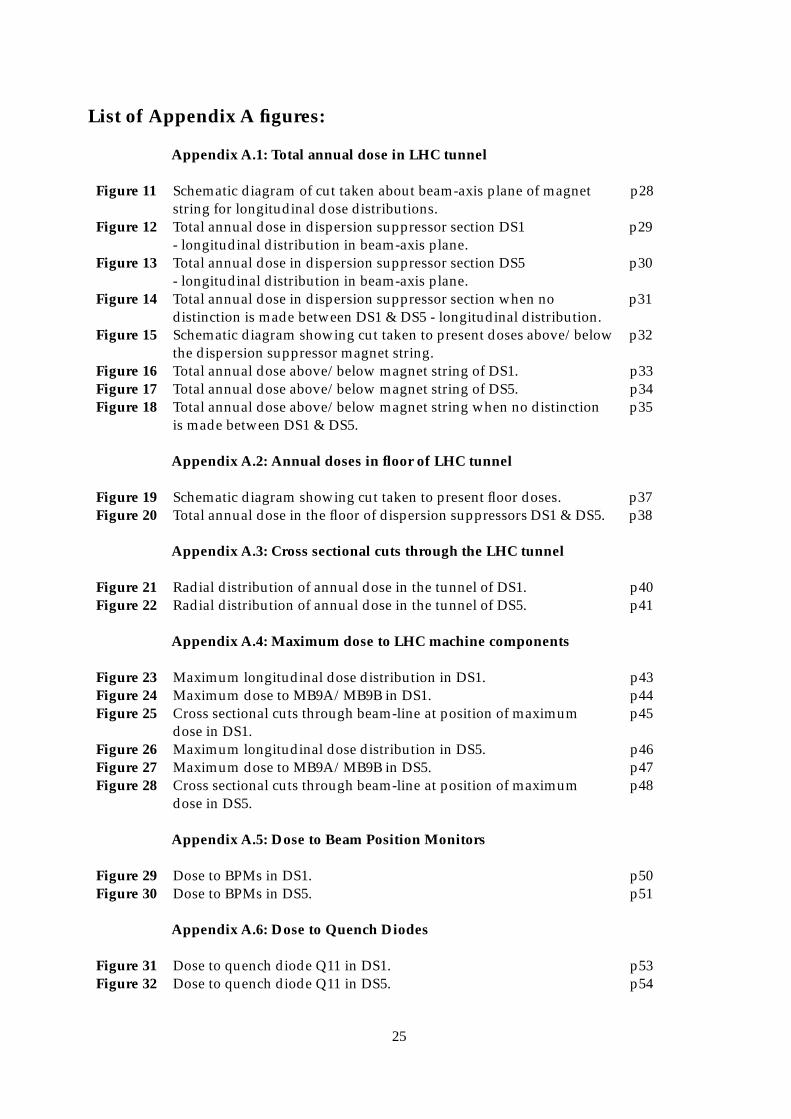
List of Appendix A figures:

Appendix A.1: Total annual dose in LHC tunnel

Figure 11 Schematic diagram of cut taken about beam-axis plane of magnet p28string for longitudinal dose distributions.

Figure 12 Total annual dose in dispersion suppressor section DS1 p29- longitudinal distribution in beam-axis plane.

Figure 13 Total annual dose in dispersion suppressor section DS5 p30- longitudinal distribution in beam-axis plane.

Figure 14 Total annual dose in dispersion suppressor section when no p31distinction is made between DS1 & DS5 - longitudinal distribution.

Figure 15 Schematic diagram showing cut taken to present doses above/below p32the dispersion suppressor magnet string.

Figure 16 Total annual dose above/below magnet string of DS1. p33Figure 17 Total annual dose above/below magnet string of DS5. p34Figure 18 Total annual dose above/below magnet string when no distinction p35

is made between DS1 & DS5.

Appendix A.2: Annual doses in floor of LHC tunnel

Figure 19 Schematic diagram showing cut taken to present floor doses. p37Figure 20 Total annual dose in the floor of dispersion suppressors DS1 & DS5. p38

Appendix A.3: Cross sectional cuts through the LHC tunnel

Figure 21 Radial distribution of annual dose in the tunnel of DS1. p40Figure 22 Radial distribution of annual dose in the tunnel of DS5. p41

Appendix A.4: Maximum dose to LHC machine components

Figure 23 Maximum longitudinal dose distribution in DS1. p43Figure 24 Maximum dose to MB9A/MB9B in DS1. p44Figure 25 Cross sectional cuts through beam-line at position of maximum p45

dose in DS1.Figure 26 Maximum longitudinal dose distribution in DS5. p46Figure 27 Maximum dose to MB9A/MB9B in DS5. p47Figure 28 Cross sectional cuts through beam-line at position of maximum p48

dose in DS5.

Appendix A.5: Dose to Beam Position Monitors

Figure 29 Dose to BPMs in DS1. p50Figure 30 Dose to BPMs in DS5. p51

Appendix A.6: Dose to Quench Diodes

Figure 31 Dose to quench diode Q11 in DS1. p53Figure 32 Dose to quench diode Q11 in DS5. p54

25

Figure 33 Dose to dipole diode MB11A. p55Figure 34 Dose to dipole diode MB11B. p56Figure 35 Dose to dipole diode MB10A. p57Figure 36 Dose to dipole diode MB10B. p58Figure 37 Dose to dipole diode MB9A. p59Figure 38 Dose to dipole diode MB9B. p60Figure 39 Dose to dipole diode MB8A. p61Figure 40 Dose to dipole diode MB8B. p62

List of Appendix B figures:

Appendix B.1: Fluence : Dose ratios above/below the magnet string

Figure 41 Neutron fluence : dose ratios above/below magnet string. p65Figure 42 Proton fluence : dose ratios above/below magnet string. p67Figure 43 Charged pion fluence : dose ratios above/below magnet string. p78Figure 44 Hadron fluence : dose ratios above/below magnet string. p69

Appendix B.2: Radial fluence : dose ratio distibutions

Figure 45 Neutron fluence : dose ratio in tunnel at Q11. p72Figure 46 Hadron fluence : dose ratio in tunnel at Q11. p73Figure 47 Neutron fluence : dose ratio in tunnel at missing magnet. p74Figure 48 Hadron fluence : dose ratio in tunnel at missing magnet. p75Figure 49 Neutron fluence : dose ratio in tunnel at dipole magnet. p76Figure 50 Hadron fluence : dose ratio in tunnel at dipole magnet. p77Figure 51 Neutron fluence : dose ratio in tunnel at quadrupole magnet. p78Figure 52 Hadron fluence : dose ratio in tunnel at quadrupole magnet. p79Figure 53 Neutron fluence : dose ratio in tunnel at intermagnet gap. p80Figure 54 Hadron fluence : dose ratio in tunnel at intermagnet gap. p81

Appendix B.3: Quantitative fluence : dose ratios

Figure 55 Particle fluence : dose ratios > 100 keV. p83Figure 56 Particle fluence : dose ratios > 1 MeV. p84Figure 57 Particle fluence : dose ratios > 20 MeV. p85Figure 58 Particle fluence : dose ratios > 50 MeV. p86Figure 59 Particle fluence : dose ratios > 100 MeV. p87

26

Appendix A.1

Total annual dose due in the dispersion suppressor regionsof the high luminosity insertion points IR1 & IR5.

Tunnel Doses

27

-200

-100

0

100

200

-200 -100 0 100 200 300

Figure 11: Schematic cross-section of the tunnel in the dispersion suppressors downstream of IP1 and IP5in the LHC. In the following figures, for those depicting horizontal cuts through the tunnel geometry thedoses shown are averaged over a slice 20 cm thick about the beam-axis (shaded region above). For themaxiumum doses in the LHC tunnel (see Appendix A.4) the above slice has a thickness of 4 cm for theinner regions of the LHC magnets.

28

-10000

-8000

-6000

-4000

-2000

0

2000

4000

6000

8000

-200 -100 0 100 200 3001.0E-01

2.2E-01

4.6E-01

1.0E+00

2.2E+00

4.6E+00

1.0E+01

2.2E+01

4.6E+01

1.0E+02

2.2E+02

4.6E+02

1.0E+03

2.2E+03

4.6E+03

1.0E+04

2.2E+04

4.6E+04

1.0E+05

2.2E+05

4.6E+05

1.0E+06

Figure 12: Total annual dose in the LHC tunnel (Gy/y) due to point losses and beam-gas interactions:shown alongside the magnets in the dispersion suppressors of IR1. The outgoing protons from IP1 are inthe outer beam-pipe. The plot shows the dose for a horizontal cut averaged over a slice 20 cm about thebeam-axis (see Figure 11). The dose contribution due to point losses was obtained by weighting the FLUKAresults of dose per interacting proton by the proton loss density (red solid line) of Figure 1.

29

-10000

-8000

-6000

-4000

-2000

0

2000

4000

6000

8000

-200 -100 0 100 200 3001.0E-01

2.2E-01

4.6E-01

1.0E+00

2.2E+00

4.6E+00

1.0E+01

2.2E+01

4.6E+01

1.0E+02

2.2E+02

4.6E+02

1.0E+03

2.2E+03

4.6E+03

1.0E+04

2.2E+04

4.6E+04

1.0E+05

2.2E+05

4.6E+05

1.0E+06

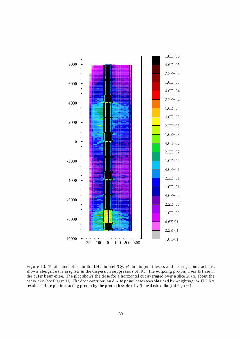
Figure 13: Total annual dose in the LHC tunnel (Gy/y) due to point losses and beam-gas interactions:shown alongside the magnets in the dispersion suppressors of IR5. The outgoing protons from IP1 are inthe outer beam-pipe. The plot shows the dose for a horizontal cut averaged over a slice 20 cm about thebeam-axis (see Figure 11). The dose contribution due to point losses was obtained by weighting the FLUKAresults of dose per interacting proton by the proton loss density (blue dashed line) of Figure 1.

30

-10000

-8000

-6000

-4000

-2000

0

2000

4000

6000

8000

-200 -100 0 100 200 3001.0E-01

2.2E-01

4.6E-01

1.0E+00

2.2E+00

4.6E+00

1.0E+01

2.2E+01

4.6E+01

1.0E+02

2.2E+02

4.6E+02

1.0E+03

2.2E+03

4.6E+03

1.0E+04

2.2E+04

4.6E+04

1.0E+05

2.2E+05

4.6E+05

1.0E+06

Figure 14: Total annual dose in the LHC tunnel (Gy/y) due to point losses and beam-gas interactions:shown alongside the magnets in the dispersion suppressors for the case when no distinction is made be-tween the beam-crossing orientations of Points 1 or 5. The outgoing protons from the IP are in the outerbeam-pipe. The plot shows the dose for a horizontal cut averaged over a slice 20 cm about the beam-axis(see Figure 11). The annual doses were obtained by weighting the FLUKA results of dose per interactingproton by the proton loss density (black double dashed line) of Figure 1.

31

-200

-100

0

100

200

-200 -100 0 100 200 300

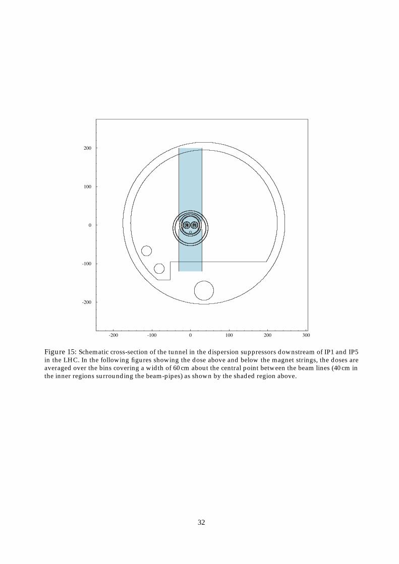
Figure 15: Schematic cross-section of the tunnel in the dispersion suppressors downstream of IP1 and IP5in the LHC. In the following figures showing the dose above and below the magnet strings, the doses areaveraged over the bins covering a width of 60 cm about the central point between the beam lines (40 cm inthe inner regions surrounding the beam-pipes) as shown by the shaded region above.

32

-100

-50

0

50

100

150

200

250

-10000 -8000 -6000 -4000 -2000 0 2000 4000 6000 8000

1.0E+6 1.0E+5 1.0E+4 1.0E+3 1.0E+2 1.0E+1 1.0E+0 1.0E-1

Figure 16: Total annual dose (Gy/y) above and below the magnet string in the dispersion suppressors ofIR1. Doses are the average over the shaded region shown in Figure 15. The annual doses were obtained byweighting the FLUKA dose per interacting proton results by the proton loss given by the red solid line ofFigure 1.

33

-100

-50

0

50

100

150

200

250

-10000 -8000 -6000 -4000 -2000 0 2000 4000 6000 8000

1.0E+6 1.0E+5 1.0E+4 1.0E+3 1.0E+2 1.0E+1 1.0E+0 1.0E-1

Figure 17: Total annual dose (Gy/y) above and below the magnet string in the dispersion suppressors ofIR5. Doses are the average over the shaded region shown in Figure 15. The annual doses were obtained byweighting the FLUKA dose per interacting proton results by the proton loss given by the blue dashed lineof Figure 1.

34

-100

-50

0

50

100

150

200

250

-10000 -8000 -6000 -4000 -2000 0 2000 4000 6000 8000

1.0E+6 1.0E+5 1.0E+4 1.0E+3 1.0E+2 1.0E+1 1.0E+0 1.0E-1

Figure 18: Total annual dose (Gy/y) above and below the magnet string in the dispersion suppressorswhen no distinction is made between the beam-crossing orientations of IP1 or IP5. Doses are the averageover the shaded region shown in Figure 15. The annual doses were obtained by weighting the FLUKA doseper interacting proton results by the proton loss given by the black double dashed line of Figure 1.

35

Appendix A.2

Total annual dose in the floor of the tunnel for DS1 & DS5

36

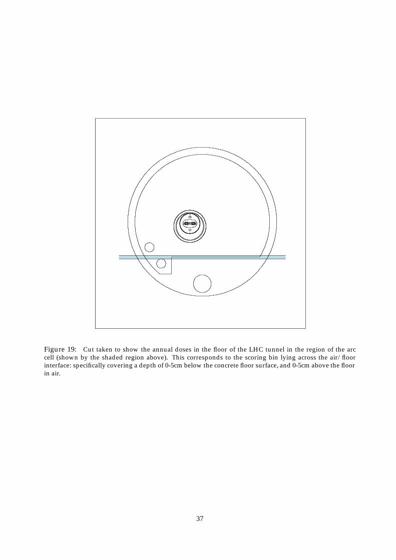
Figure 19: Cut taken to show the annual doses in the floor of the LHC tunnel in the region of the arccell (shown by the shaded region above). This corresponds to the scoring bin lying across the air/floorinterface: specifically covering a depth of 0-5cm below the concrete floor surface, and 0-5cm above the floorin air.

37

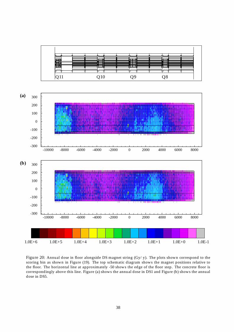
-300

-200

-100

0

100

200

300

-10000 -8000 -6000 -4000 -2000 0 2000 4000 6000 8000

-300

-200

-100

0

100

200

300

-10000 -8000 -6000 -4000 -2000 0 2000 4000 6000 8000

(a)

(b)

1.0E+6 1.0E+5 1.0E+4 1.0E+3 1.0E+2 1.0E+1 1.0E+0 1.0E-1

Q11 Q10 Q9 Q8

Figure 20: Annual dose in floor alongside DS magnet string (Gy/y). The plots shown correspond to thescoring bin as shown in Figure (19). The top schematic diagram shows the magnet positions relative tothe floor. The horizontal line at approximately -50 shows the edge of the floor step. The concrete floor iscorrespondingly above this line. Figure (a) shows the annual dose in DS1 and Figure (b) shows the annualdose in DS5.

38

Appendix A.3

Maximum dose in the LHC tunnel for the dispersionsuppressors DS1 & DS5

Cross sectional cuts through the LHC tunnel

39

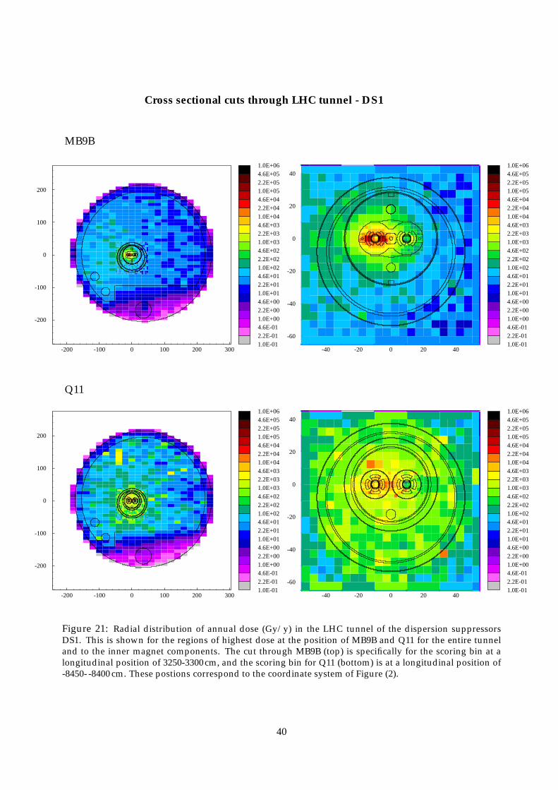
Cross sectional cuts through LHC tunnel - DS1

MB9B

-200

-100

0

100

200

-200 -100 0 100 200 3001.0E-012.2E-014.6E-011.0E+002.2E+004.6E+001.0E+012.2E+014.6E+011.0E+022.2E+024.6E+021.0E+032.2E+034.6E+031.0E+042.2E+044.6E+041.0E+052.2E+054.6E+051.0E+06

-60

-40

-20

0

20

40

-40 -20 0 20 401.0E-012.2E-014.6E-011.0E+002.2E+004.6E+001.0E+012.2E+014.6E+011.0E+022.2E+024.6E+021.0E+032.2E+034.6E+031.0E+042.2E+044.6E+041.0E+052.2E+054.6E+051.0E+06

Q11

-200

-100

0

100

200

-200 -100 0 100 200 3001.0E-012.2E-014.6E-011.0E+002.2E+004.6E+001.0E+012.2E+014.6E+011.0E+022.2E+024.6E+021.0E+032.2E+034.6E+031.0E+042.2E+044.6E+041.0E+052.2E+054.6E+051.0E+06

-60

-40

-20

0

20

40

-40 -20 0 20 401.0E-012.2E-014.6E-011.0E+002.2E+004.6E+001.0E+012.2E+014.6E+011.0E+022.2E+024.6E+021.0E+032.2E+034.6E+031.0E+042.2E+044.6E+041.0E+052.2E+054.6E+051.0E+06

Figure 21: Radial distribution of annual dose (Gy/y) in the LHC tunnel of the dispersion suppressorsDS1. This is shown for the regions of highest dose at the position of MB9B and Q11 for the entire tunneland to the inner magnet components. The cut through MB9B (top) is specifically for the scoring bin at alongitudinal position of 3250-3300cm, and the scoring bin for Q11 (bottom) is at a longitudinal position of-8450- -8400 cm. These postions correspond to the coordinate system of Figure (2).

40

Cross sectional cuts through LHC tunnel - DS5

MB9B

-200

-100

0

100

200

-200 -100 0 100 200 3001.0E-012.2E-014.6E-011.0E+002.2E+004.6E+001.0E+012.2E+014.6E+011.0E+022.2E+024.6E+021.0E+032.2E+034.6E+031.0E+042.2E+044.6E+041.0E+052.2E+054.6E+051.0E+06

-60

-40

-20

0

20

40

-40 -20 0 20 401.0E-012.2E-014.6E-011.0E+002.2E+004.6E+001.0E+012.2E+014.6E+011.0E+022.2E+024.6E+021.0E+032.2E+034.6E+031.0E+042.2E+044.6E+041.0E+052.2E+054.6E+051.0E+06

Q11

-200

-100

0

100

200

-200 -100 0 100 200 3001.0E-012.2E-014.6E-011.0E+002.2E+004.6E+001.0E+012.2E+014.6E+011.0E+022.2E+024.6E+021.0E+032.2E+034.6E+031.0E+042.2E+044.6E+041.0E+052.2E+054.6E+051.0E+06

-60

-40

-20

0

20

40

-40 -20 0 20 401.0E-012.2E-014.6E-011.0E+002.2E+004.6E+001.0E+012.2E+014.6E+011.0E+022.2E+024.6E+021.0E+032.2E+034.6E+031.0E+042.2E+044.6E+041.0E+052.2E+054.6E+051.0E+06

Figure 22: Radial distribution of annual dose (Gy/y) in the LHC tunnel of the dispersion suppressorsDS5. This is shown for the regions of highest dose at the position of MB9B and Q11 for the entire tunneland to the inner magnet components. The cut through MB9B (top) is specifically for the scoring bin at alongitudinal position of 3250-3300cm, and the scoring bin for Q11 (bottom) is at a longitudinal position of-8450- -8400 cm. These postions correspond to the coordinate system of Figure (2).

41

Appendix A.4

Maximum dose in the inner regions of the dispersion suppressor magnetsof the high luminosity insertion points IR1 & IR5.

Dose to beamline and magnet coils

42

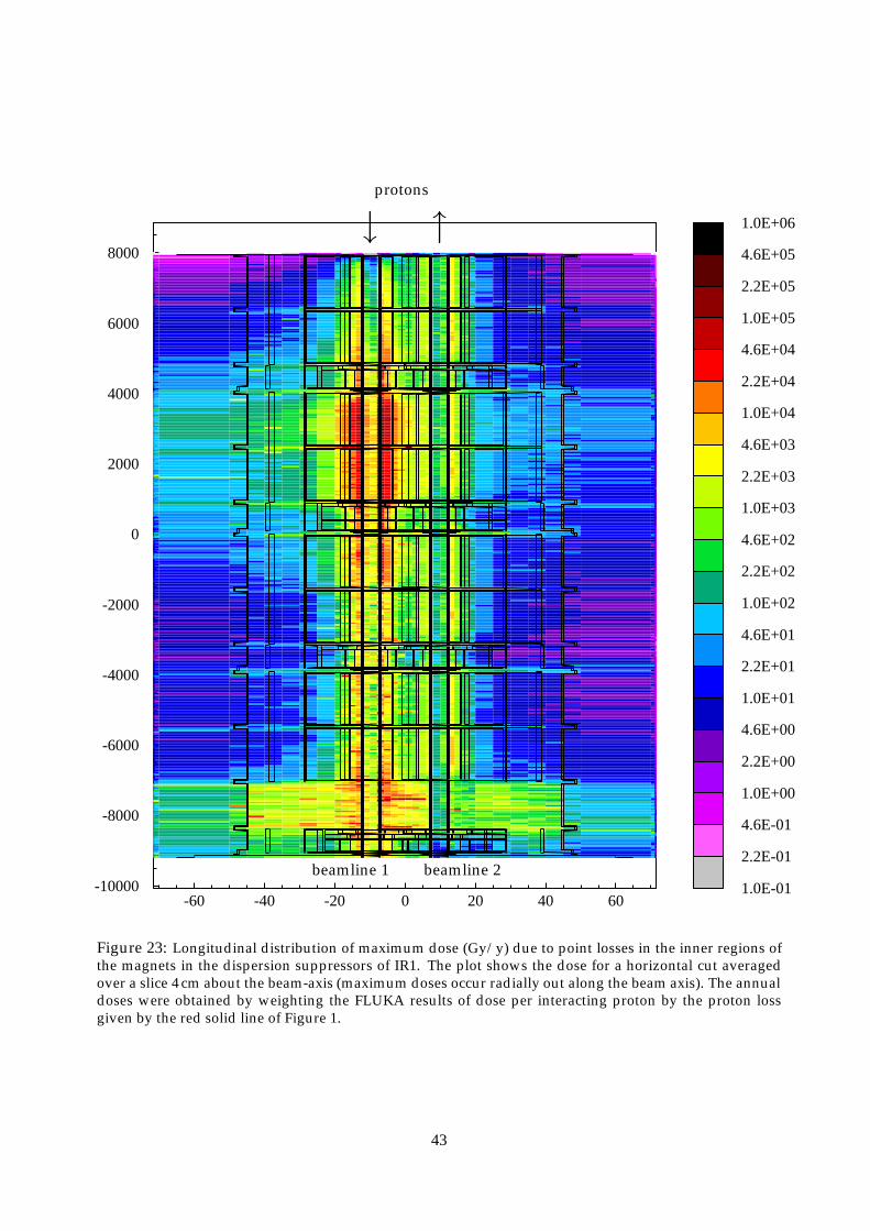
-10000

-8000

-6000

-4000

-2000

0

2000

4000

6000

8000

-60 -40 -20 0 20 40 601.0E-01

2.2E-01

4.6E-01

1.0E+00

2.2E+00

4.6E+00

1.0E+01

2.2E+01

4.6E+01

1.0E+02

2.2E+02

4.6E+02

1.0E+03

2.2E+03

4.6E+03

1.0E+04

2.2E+04

4.6E+04

1.0E+05

2.2E+05

4.6E+05

1.0E+06

protons

↓ ↑

beamline 1 beamline 2

Figure 23: Longitudinal distribution of maximum dose (Gy/y) due to point losses in the inner regions ofthe magnets in the dispersion suppressors of IR1. The plot shows the dose for a horizontal cut averagedover a slice 4 cm about the beam-axis (maximum doses occur radially out along the beam axis). The annualdoses were obtained by weighting the FLUKA results of dose per interacting proton by the proton lossgiven by the red solid line of Figure 1.

43

500

1000

1500

2000

2500

3000

3500

4000

4500

-25 -20 -15 -10 -5 01.0E-01

2.2E-01

4.6E-01

1.0E+00

2.2E+00

4.6E+00

1.0E+01

2.2E+01

4.6E+01

1.0E+02

2.2E+02

4.6E+02

1.0E+03

2.2E+03

4.6E+03

1.0E+04

2.2E+04

4.6E+04

1.0E+05

2.2E+05

4.6E+05

1.0E+06

MB9B

MB9A

Figure 24: Maximum annual dose (Gy/y) in the inner regions of the dipole magnets MB9A/MB9B in thedispersion suppressors of IR1 - specifically covering beamline 1 and the surrounding dipole coils (enlarge-ment of inner section of magnets from Figure 21). The plot shows the dose for a horizontal cut averagedover a slice 4 cm about the beam-axis. The point loss contribution was obtained by weighting the FLUKAresults of dose per interacting proton by the proton loss given by the red solid line of Figure 1.

44

2000 2250 2500 2750 3000 3250 3500 3750 4000

a b c d e f

MB9A→←MB9B · · ·

-6

-4

-2

0

2

4

6

-16 -14 -12 -10 -8 -6 -4

-6

-4

-2

0

2

4

6

-16 -14 -12 -10 -8 -6 -4

-6

-4

-2

0

2

4

6

-16 -14 -12 -10 -8 -6 -4

-6

-4

-2

0

2

4

6

-16 -14 -12 -10 -8 -6 -4

-6

-4

-2

0

2

4

6

-16 -14 -12 -10 -8 -6 -4

-6

-4

-2

0

2

4

6

-16 -14 -12 -10 -8 -6 -4

1.0E+6 1.0E+5 1.0E+4 1.0E+3 1.0E+2 1.0E+1 1.0E+0 1.0E-1

a b c

d e f

Figure 25: Selection of cross-sectional slices showing maximum dose (Gy/y) in the coils and beam-line of the dipole magnet MB9B in the dispersion suppressors of IR1. This is for the outgoingproton direction beam-line. The proton loss distribution used is taken from [Bai00] for a rate of3.5× 108 inelastic interactions per second in the IP. The total proton loss in IR1 is 1.1 × 107 s−1.Each slice corresponds to the labelled slice in the top schematic diagram.

45

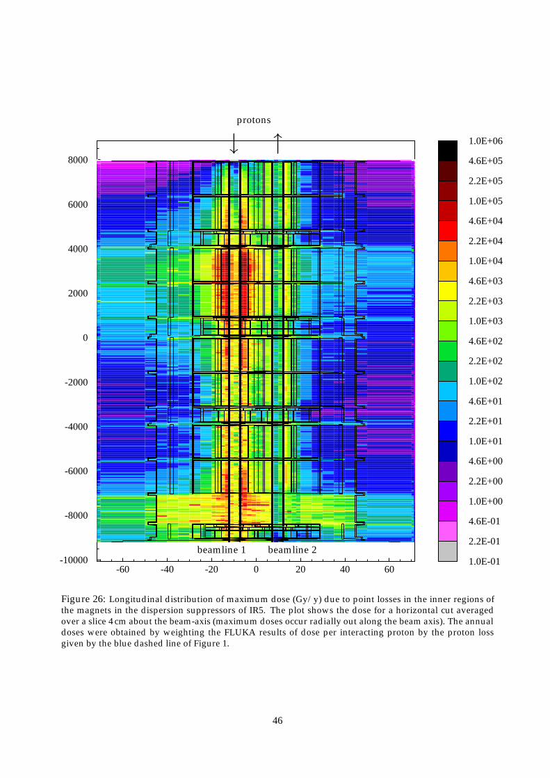
-10000

-8000

-6000

-4000

-2000

0

2000

4000

6000

8000

-60 -40 -20 0 20 40 601.0E-01

2.2E-01

4.6E-01

1.0E+00

2.2E+00

4.6E+00

1.0E+01

2.2E+01

4.6E+01

1.0E+02

2.2E+02

4.6E+02

1.0E+03

2.2E+03

4.6E+03

1.0E+04

2.2E+04

4.6E+04

1.0E+05

2.2E+05

4.6E+05

1.0E+06

protons

↓ ↑

beamline 1 beamline 2

Figure 26: Longitudinal distribution of maximum dose (Gy/y) due to point losses in the inner regions ofthe magnets in the dispersion suppressors of IR5. The plot shows the dose for a horizontal cut averagedover a slice 4 cm about the beam-axis (maximum doses occur radially out along the beam axis). The annualdoses were obtained by weighting the FLUKA results of dose per interacting proton by the proton lossgiven by the blue dashed line of Figure 1.

46

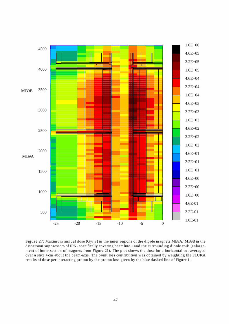
500

1000

1500

2000

2500

3000

3500

4000

4500

-25 -20 -15 -10 -5 01.0E-01

2.2E-01

4.6E-01

1.0E+00

2.2E+00

4.6E+00

1.0E+01

2.2E+01

4.6E+01

1.0E+02

2.2E+02

4.6E+02

1.0E+03

2.2E+03

4.6E+03

1.0E+04

2.2E+04

4.6E+04

1.0E+05

2.2E+05

4.6E+05

1.0E+06

MB9B

MB9A

Figure 27: Maximum annual dose (Gy/y) in the inner regions of the dipole magnets MB9A/MB9B in thedispersion suppressors of IR5 - specifically covering beamline 1 and the surrounding dipole coils (enlarge-ment of inner section of magnets from Figure 21). The plot shows the dose for a horizontal cut averagedover a slice 4 cm about the beam-axis. The point loss contribution was obtained by weighting the FLUKAresults of dose per interacting proton by the proton loss given by the blue dashed line of Figure 1.

47

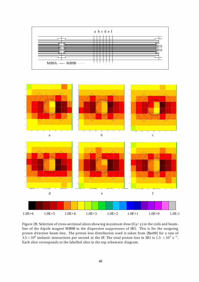
2000 2250 2500 2750 3000 3250 3500 3750 4000

a b c d e f

MB9A→←MB9B · · ·

-6

-4

-2

0

2

4

6

-16 -14 -12 -10 -8 -6 -4

-6

-4

-2

0

2

4

6

-16 -14 -12 -10 -8 -6 -4

-6

-4

-2

0

2

4

6

-16 -14 -12 -10 -8 -6 -4

-6

-4

-2

0

2

4

6

-16 -14 -12 -10 -8 -6 -4

-6

-4

-2

0

2

4

6

-16 -14 -12 -10 -8 -6 -4

-6

-4

-2

0

2

4

6

-16 -14 -12 -10 -8 -6 -4

1.0E+6 1.0E+5 1.0E+4 1.0E+3 1.0E+2 1.0E+1 1.0E+0 1.0E-1

a b c

d e f

Figure 28: Selection of cross-sectional slices showing maximum dose (Gy/y) in the coils and beam-line of the dipole magnet MB9B in the dispersion suppressors of IR5. This is for the outgoingproton direction beam-line. The proton loss distribution used is taken from [Bai00] for a rate of3.5× 108 inelastic interactions per second in the IP. The total proton loss in IR1 is 1.3 × 107 s−1.Each slice corresponds to the labelled slice in the top schematic diagram.

48

Appendix A.5

Annual dose to the beam position monitors (Q8-Q11)

49

-60

-40

-20

0

20

40

60

4040 4060 4080 4100 4120 4140 4160

-60

-40

-20

0

20

40

60

-20 0 20 40 60 80 100 120

-60

-40

-20

0

20

40

60

-3920 -3900 -3880 -3860 -3840 -3820 -3800

-60

-40

-20

0

20

40

60

-9160 -9140 -9120 -9100 -9080 -9060 -9040

1.0E+6 1.0E+5 1.0E+4 1.0E+3 1.0E+2 1.0E+1 1.0E+0 1.0E-1

Beam Position Monitors in Dispersion Suppressors IR1

(a) BPM: Q8 (b) BPM: Q9

(c) BPM: Q10 (d) BPM: Q11

Figure 29: Dose (Gy/y) to the Beam Position Monitors: (a) Q8, (b) Q9, (c) Q10 and (d) Q11 in the dispersionsuppressors of IR1. These doses are averaged over a slice of 12cm around the beam-axis covering the radialextent of the BPM. In Figure (d) contributions to the dose from beam-gas interactions and from the upstreamarcs are missing due to the start of the FLUKA geometry at this point. Realistic doses for the second beam-pipe would appear similar to those shown in Figures (a)-(c).

50

-60

-40

-20

0

20

40

60

4040 4060 4080 4100 4120 4140 4160

-60

-40

-20

0

20

40

60

-20 0 20 40 60 80 100 120

-60

-40

-20

0

20

40

60

-3920 -3900 -3880 -3860 -3840 -3820 -3800

-60

-40

-20

0

20

40

60

-9160 -9140 -9120 -9100 -9080 -9060 -9040

1.0E+6 1.0E+5 1.0E+4 1.0E+3 1.0E+2 1.0E+1 1.0E+0 1.0E-1

Beam Position Monitors in Dispersion Suppressors IR5

(a) BPM: Q8 (b) BPM: Q9

(c) BPM: Q10 (d) BPM: Q11

Figure 30: Dose (Gy/y) to the Beam Position Monitors: (a) Q8, (b) Q9, (c) Q10 and (d) Q11 in the dispersionsuppressors of IR5 due to point losses. These doses are averaged over a slice of 12cm around the beam-axiscovering the radial extent of the BPM. In Figure (d) contributions to the dose from beam-gas interactionsand from the upstream arcs are missing due to the start of the FLUKA geometry at this point. Realisticdoses for the second beam-pipe would appear similar to those shown in Figures (a)-(c).

51

Appendix A.6

Annual dose to the quench diodes in the dispersion suppressors of thehigh luminosity insertion points IR1 & IR5

52

Dispersion Suppressor Pt1 - diode Q11

-60

-40

-20

0

20

40

60

-60 -40 -20 0 20 40 601.0E-012.2E-014.6E-011.0E+002.2E+004.6E+001.0E+012.2E+014.6E+011.0E+022.2E+024.6E+021.0E+032.2E+034.6E+031.0E+042.2E+044.6E+041.0E+052.2E+054.6E+051.0E+06

-60

-40

-20

0

20

40

60

-60 -40 -20 0 20 40 601.0E-012.2E-014.6E-011.0E+002.2E+004.6E+001.0E+012.2E+014.6E+011.0E+022.2E+024.6E+021.0E+032.2E+034.6E+031.0E+042.2E+044.6E+041.0E+052.2E+054.6E+051.0E+06

-50

-40

-30

-20

-10

0

10

20

-9130 -9120 -9110 -9100 -9090 -9080 -9070 -90601.0E-012.2E-014.6E-011.0E+002.2E+004.6E+001.0E+012.2E+014.6E+011.0E+022.2E+024.6E+021.0E+032.2E+034.6E+031.0E+042.2E+044.6E+041.0E+052.2E+054.6E+051.0E+06

(a) cross section x: Si wafer 1 (b) cross section y: Si wafer 2

(c) longitudinal dose distribution over quadrupolediode

↑ ↑x y

Figure 31: Dose (Gy/y) to the quadrupole diode of Q11 in the dispersion suppressors of IR1. The thinstrips labelled “x” and “y” represents the Si in the diode. Plots (a) and (b) show cross sectional cuts throughthe Si wafer strips x and y respectively. Plot (c) shows the longitudinal dose distribution averaged over thewidth of the diode housing region.

53

Dispersion Suppressor Pt5 - diode Q11

-60

-40

-20

0

20

40

60

-60 -40 -20 0 20 40 601.0E-012.2E-014.6E-011.0E+002.2E+004.6E+001.0E+012.2E+014.6E+011.0E+022.2E+024.6E+021.0E+032.2E+034.6E+031.0E+042.2E+044.6E+041.0E+052.2E+054.6E+051.0E+06

-60

-40

-20

0

20

40

60

-60 -40 -20 0 20 40 601.0E-012.2E-014.6E-011.0E+002.2E+004.6E+001.0E+012.2E+014.6E+011.0E+022.2E+024.6E+021.0E+032.2E+034.6E+031.0E+042.2E+044.6E+041.0E+052.2E+054.6E+051.0E+06

-50

-40

-30

-20

-10

0

10

20

-9130 -9120 -9110 -9100 -9090 -9080 -9070 -90601.0E-012.2E-014.6E-011.0E+002.2E+004.6E+001.0E+012.2E+014.6E+011.0E+022.2E+024.6E+021.0E+032.2E+034.6E+031.0E+042.2E+044.6E+041.0E+052.2E+054.6E+051.0E+06

(a) cross section x: Si wafer 1 (b) cross section y: Si wafer 2

(c) longitudinal dose distribution over quadrupolediode

↑ ↑x y

Figure 32: Dose (Gy/y) to the quadrupole diode of Q11 in the dispersion suppressors of IR5 due to pointlosses. The thin strips labelled “x” and “y” represents the Si in the diode. Plots (a) and (b) show cross sec-tional cuts through the Si wafer strips x and y respectively. Plot (c) shows the longitudinal dose distributionaveraged over the width of the diode housing region.

54

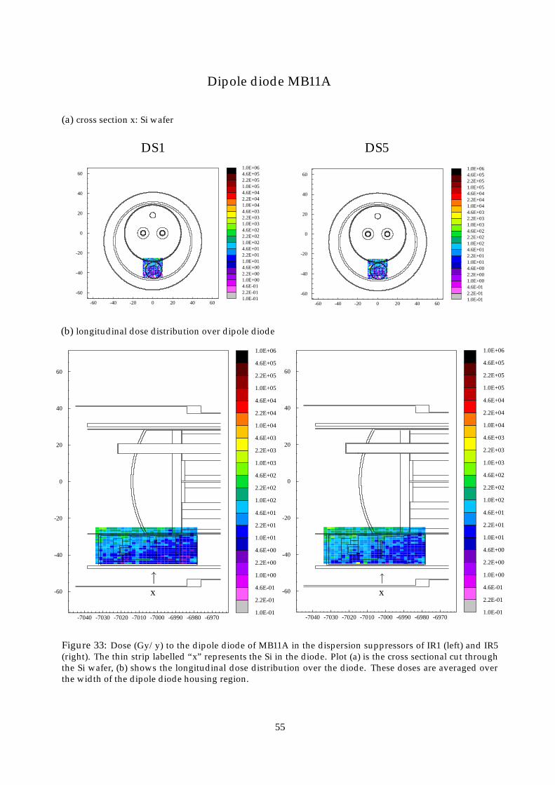
Dipole diode MB11A

-60

-40

-20

0

20

40

60

-60 -40 -20 0 20 40 601.0E-012.2E-014.6E-011.0E+002.2E+004.6E+001.0E+012.2E+014.6E+011.0E+022.2E+024.6E+021.0E+032.2E+034.6E+031.0E+042.2E+044.6E+041.0E+052.2E+054.6E+051.0E+06

-60

-40

-20

0

20

40

60

-60 -40 -20 0 20 40 601.0E-012.2E-014.6E-011.0E+002.2E+004.6E+001.0E+012.2E+014.6E+011.0E+022.2E+024.6E+021.0E+032.2E+034.6E+031.0E+042.2E+044.6E+041.0E+052.2E+054.6E+051.0E+06

-60

-40

-20

0

20

40

60

-7040 -7030 -7020 -7010 -7000 -6990 -6980 -69701.0E-01

2.2E-01

4.6E-01

1.0E+00

2.2E+00

4.6E+00

1.0E+01

2.2E+01

4.6E+01

1.0E+02

2.2E+02

4.6E+02

1.0E+03

2.2E+03

4.6E+03

1.0E+04

2.2E+04

4.6E+04

1.0E+05

2.2E+05

4.6E+05

1.0E+06

-60

-40

-20

0

20

40

60

-7040 -7030 -7020 -7010 -7000 -6990 -6980 -69701.0E-01

2.2E-01

4.6E-01

1.0E+00

2.2E+00

4.6E+00

1.0E+01

2.2E+01

4.6E+01

1.0E+02

2.2E+02

4.6E+02

1.0E+03

2.2E+03

4.6E+03

1.0E+04

2.2E+04

4.6E+04

1.0E+05

2.2E+05

4.6E+05

1.0E+06

(a) cross section x: Si wafer

(b) longitudinal dose distribution over dipole diode

↑ ↑x x

DS1 DS5

Figure 33: Dose (Gy/y) to the dipole diode of MB11A in the dispersion suppressors of IR1 (left) and IR5(right). The thin strip labelled “x” represents the Si in the diode. Plot (a) is the cross sectional cut throughthe Si wafer, (b) shows the longitudinal dose distribution over the diode. These doses are averaged overthe width of the dipole diode housing region.

55

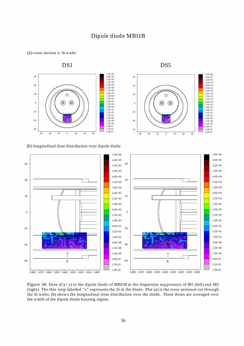
Dipole diode MB11B

-60

-40

-20

0

20

40

60

-60 -40 -20 0 20 40 601.0E-012.2E-014.6E-011.0E+002.2E+004.6E+001.0E+012.2E+014.6E+011.0E+022.2E+024.6E+021.0E+032.2E+034.6E+031.0E+042.2E+044.6E+041.0E+052.2E+054.6E+051.0E+06

-60

-40

-20

0

20

40

60

-60 -40 -20 0 20 40 601.0E-012.2E-014.6E-011.0E+002.2E+004.6E+001.0E+012.2E+014.6E+011.0E+022.2E+024.6E+021.0E+032.2E+034.6E+031.0E+042.2E+044.6E+041.0E+052.2E+054.6E+051.0E+06

-60

-40

-20

0

20

40

60

-5480 -5470 -5460 -5450 -5440 -5430 -5420 -5410 -54001.0E-01

2.2E-01

4.6E-01

1.0E+00

2.2E+00

4.6E+00

1.0E+01

2.2E+01

4.6E+01

1.0E+02

2.2E+02

4.6E+02

1.0E+03

2.2E+03

4.6E+03

1.0E+04

2.2E+04

4.6E+04

1.0E+05

2.2E+05

4.6E+05

1.0E+06

-60

-40

-20

0

20

40

60

-5480 -5470 -5460 -5450 -5440 -5430 -5420 -5410 -54001.0E-01

2.2E-01

4.6E-01

1.0E+00

2.2E+00

4.6E+00

1.0E+01

2.2E+01

4.6E+01

1.0E+02

2.2E+02

4.6E+02

1.0E+03

2.2E+03

4.6E+03

1.0E+04

2.2E+04

4.6E+04

1.0E+05

2.2E+05

4.6E+05

1.0E+06

(a) cross section x: Si wafer

(b) longitudinal dose distribution over dipole diode

↑ ↑x x

DS1 DS5

Figure 34: Dose (Gy/y) to the dipole diode of MB11B in the dispersion suppressors of IR1 (left) and IR5(right). The thin strip labelled “x” represents the Si in the diode. Plot (a) is the cross sectional cut throughthe Si wafer, (b) shows the longitudinal dose distribution over the diode. These doses are averaged overthe width of the dipole diode housing region.

56

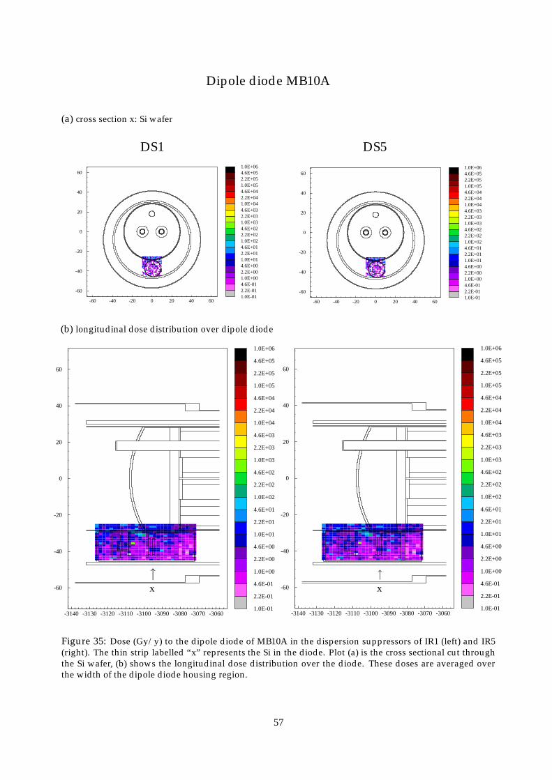
Dipole diode MB10A

-60

-40

-20

0

20

40

60

-60 -40 -20 0 20 40 601.0E-012.2E-014.6E-011.0E+002.2E+004.6E+001.0E+012.2E+014.6E+011.0E+022.2E+024.6E+021.0E+032.2E+034.6E+031.0E+042.2E+044.6E+041.0E+052.2E+054.6E+051.0E+06

-60

-40

-20

0

20

40

60

-60 -40 -20 0 20 40 601.0E-012.2E-014.6E-011.0E+002.2E+004.6E+001.0E+012.2E+014.6E+011.0E+022.2E+024.6E+021.0E+032.2E+034.6E+031.0E+042.2E+044.6E+041.0E+052.2E+054.6E+051.0E+06

-60

-40

-20

0

20

40

60

-3140 -3130 -3120 -3110 -3100 -3090 -3080 -3070 -30601.0E-01

2.2E-01

4.6E-01

1.0E+00

2.2E+00

4.6E+00

1.0E+01

2.2E+01

4.6E+01

1.0E+02

2.2E+02

4.6E+02

1.0E+03

2.2E+03

4.6E+03

1.0E+04

2.2E+04

4.6E+04

1.0E+05

2.2E+05

4.6E+05

1.0E+06

-60

-40

-20

0

20

40

60

-3140 -3130 -3120 -3110 -3100 -3090 -3080 -3070 -30601.0E-01

2.2E-01

4.6E-01

1.0E+00

2.2E+00

4.6E+00

1.0E+01

2.2E+01

4.6E+01

1.0E+02

2.2E+02

4.6E+02

1.0E+03

2.2E+03

4.6E+03

1.0E+04

2.2E+04

4.6E+04

1.0E+05

2.2E+05

4.6E+05

1.0E+06

(a) cross section x: Si wafer

(b) longitudinal dose distribution over dipole diode

↑ ↑x x

DS1 DS5

Figure 35: Dose (Gy/y) to the dipole diode of MB10A in the dispersion suppressors of IR1 (left) and IR5(right). The thin strip labelled “x” represents the Si in the diode. Plot (a) is the cross sectional cut throughthe Si wafer, (b) shows the longitudinal dose distribution over the diode. These doses are averaged overthe width of the dipole diode housing region.

57

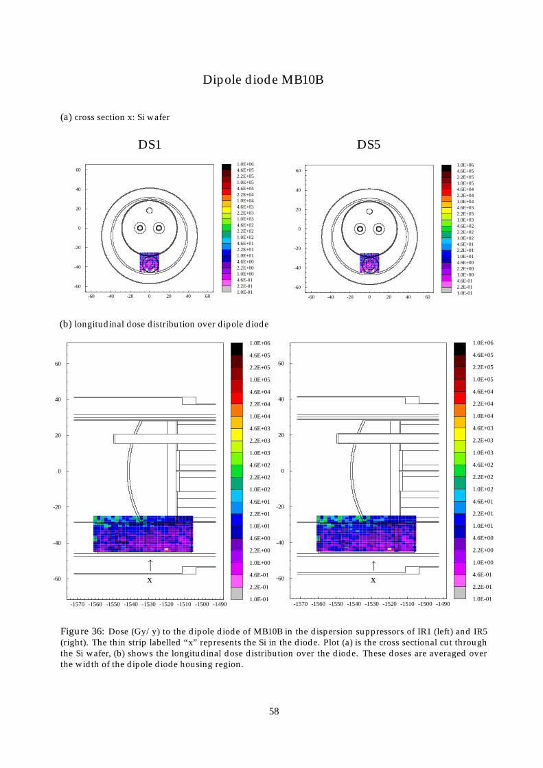
Dipole diode MB10B

-60

-40

-20

0

20

40

60

-60 -40 -20 0 20 40 601.0E-012.2E-014.6E-011.0E+002.2E+004.6E+001.0E+012.2E+014.6E+011.0E+022.2E+024.6E+021.0E+032.2E+034.6E+031.0E+042.2E+044.6E+041.0E+052.2E+054.6E+051.0E+06

-60

-40

-20

0

20

40

60

-60 -40 -20 0 20 40 601.0E-012.2E-014.6E-011.0E+002.2E+004.6E+001.0E+012.2E+014.6E+011.0E+022.2E+024.6E+021.0E+032.2E+034.6E+031.0E+042.2E+044.6E+041.0E+052.2E+054.6E+051.0E+06

-60

-40

-20

0

20

40

60

-1570 -1560 -1550 -1540 -1530 -1520 -1510 -1500 -14901.0E-01

2.2E-01

4.6E-01

1.0E+00

2.2E+00

4.6E+00

1.0E+01

2.2E+01

4.6E+01

1.0E+02

2.2E+02

4.6E+02

1.0E+03

2.2E+03

4.6E+03

1.0E+04

2.2E+04

4.6E+04

1.0E+05

2.2E+05

4.6E+05

1.0E+06

-60

-40

-20

0

20

40

60

-1570 -1560 -1550 -1540 -1530 -1520 -1510 -1500 -14901.0E-01

2.2E-01

4.6E-01

1.0E+00

2.2E+00

4.6E+00

1.0E+01

2.2E+01

4.6E+01

1.0E+02

2.2E+02

4.6E+02

1.0E+03

2.2E+03

4.6E+03

1.0E+04

2.2E+04

4.6E+04

1.0E+05

2.2E+05

4.6E+05

1.0E+06

(a) cross section x: Si wafer

(b) longitudinal dose distribution over dipole diode

↑ ↑x x

DS1 DS5

Figure 36: Dose (Gy/y) to the dipole diode of MB10B in the dispersion suppressors of IR1 (left) and IR5(right). The thin strip labelled “x” represents the Si in the diode. Plot (a) is the cross sectional cut throughthe Si wafer, (b) shows the longitudinal dose distribution over the diode. These doses are averaged overthe width of the dipole diode housing region.

58

Dipole diode MB9A

-60

-40

-20

0

20

40

60

-60 -40 -20 0 20 40 601.0E-012.2E-014.6E-011.0E+002.2E+004.6E+001.0E+012.2E+014.6E+011.0E+022.2E+024.6E+021.0E+032.2E+034.6E+031.0E+042.2E+044.6E+041.0E+052.2E+054.6E+051.0E+06

-60

-40

-20

0

20

40

60

-60 -40 -20 0 20 40 601.0E-012.2E-014.6E-011.0E+002.2E+004.6E+001.0E+012.2E+014.6E+011.0E+022.2E+024.6E+021.0E+032.2E+034.6E+031.0E+042.2E+044.6E+041.0E+052.2E+054.6E+051.0E+06

-60

-40

-20

0

20

40

60

910 920 930 940 950 960 970 980 9901.0E-01

2.2E-01

4.6E-01

1.0E+00

2.2E+00

4.6E+00

1.0E+01

2.2E+01

4.6E+01

1.0E+02

2.2E+02

4.6E+02

1.0E+03

2.2E+03

4.6E+03

1.0E+04

2.2E+04

4.6E+04

1.0E+05

2.2E+05

4.6E+05

1.0E+06

-60

-40

-20

0

20

40

60

910 920 930 940 950 960 970 980 9901.0E-01

2.2E-01

4.6E-01

1.0E+00

2.2E+00

4.6E+00

1.0E+01

2.2E+01

4.6E+01

1.0E+02

2.2E+02

4.6E+02

1.0E+03

2.2E+03

4.6E+03

1.0E+04

2.2E+04

4.6E+04

1.0E+05

2.2E+05

4.6E+05

1.0E+06

(a) cross section x: Si wafer

(b) longitudinal dose distribution over dipole diode

↑ ↑x x

DS1 DS5

Figure 37: Dose (Gy/y) to the dipole diode of MB9A in the dispersion suppressors of IR1 (left) and IR5(right). The thin strip labelled “x” represents the Si in the diode. Plot (a) is the cross sectional cut throughthe Si wafer, (b) shows the longitudinal dose distribution over the diode. These doses are averaged overthe width of the dipole diode housing region.

59

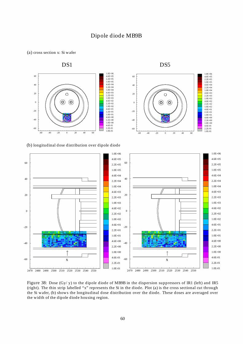
Dipole diode MB9B

-60

-40

-20

0

20

40

60

-60 -40 -20 0 20 40 601.0E-012.2E-014.6E-011.0E+002.2E+004.6E+001.0E+012.2E+014.6E+011.0E+022.2E+024.6E+021.0E+032.2E+034.6E+031.0E+042.2E+044.6E+041.0E+052.2E+054.6E+051.0E+06

-60

-40

-20

0

20

40

60

-60 -40 -20 0 20 40 601.0E-012.2E-014.6E-011.0E+002.2E+004.6E+001.0E+012.2E+014.6E+011.0E+022.2E+024.6E+021.0E+032.2E+034.6E+031.0E+042.2E+044.6E+041.0E+052.2E+054.6E+051.0E+06

-60

-40

-20

0

20

40

60

2470 2480 2490 2500 2510 2520 2530 2540 25501.0E-01

2.2E-01

4.6E-01

1.0E+00

2.2E+00

4.6E+00

1.0E+01

2.2E+01

4.6E+01

1.0E+02

2.2E+02

4.6E+02

1.0E+03

2.2E+03

4.6E+03

1.0E+04

2.2E+04

4.6E+04

1.0E+05

2.2E+05

4.6E+05

1.0E+06

-60

-40

-20

0

20

40

60

2470 2480 2490 2500 2510 2520 2530 2540 25501.0E-01

2.2E-01

4.6E-01

1.0E+00

2.2E+00

4.6E+00

1.0E+01

2.2E+01

4.6E+01

1.0E+02

2.2E+02

4.6E+02

1.0E+03

2.2E+03

4.6E+03

1.0E+04

2.2E+04

4.6E+04

1.0E+05

2.2E+05

4.6E+05

1.0E+06

(a) cross section x: Si wafer

(b) longitudinal dose distribution over dipole diode

↑ ↑x x

DS1 DS5

Figure 38: Dose (Gy/y) to the dipole diode of MB9B in the dispersion suppressors of IR1 (left) and IR5(right). The thin strip labelled “x” represents the Si in the diode. Plot (a) is the cross sectional cut throughthe Si wafer, (b) shows the longitudinal dose distribution over the diode. These doses are averaged overthe width of the dipole diode housing region.

60

Dipole diode MB8A

-60

-40

-20

0

20

40

60

-60 -40 -20 0 20 40 601.0E-012.2E-014.6E-011.0E+002.2E+004.6E+001.0E+012.2E+014.6E+011.0E+022.2E+024.6E+021.0E+032.2E+034.6E+031.0E+042.2E+044.6E+041.0E+052.2E+054.6E+051.0E+06

-60

-40

-20

0

20

40

60

-60 -40 -20 0 20 40 601.0E-012.2E-014.6E-011.0E+002.2E+004.6E+001.0E+012.2E+014.6E+011.0E+022.2E+024.6E+021.0E+032.2E+034.6E+031.0E+042.2E+044.6E+041.0E+052.2E+054.6E+051.0E+06

-60

-40

-20

0

20

40

60

4810 4820 4830 4840 4850 4860 4870 4880 48901.0E-01

2.2E-01

4.6E-01

1.0E+00

2.2E+00

4.6E+00

1.0E+01

2.2E+01

4.6E+01

1.0E+02

2.2E+02

4.6E+02

1.0E+03

2.2E+03

4.6E+03

1.0E+04

2.2E+04

4.6E+04

1.0E+05

2.2E+05

4.6E+05

1.0E+06

-60

-40

-20

0

20

40

60

4810 4820 4830 4840 4850 4860 4870 4880 48901.0E-01

2.2E-01

4.6E-01

1.0E+00

2.2E+00

4.6E+00

1.0E+01

2.2E+01

4.6E+01

1.0E+02

2.2E+02

4.6E+02

1.0E+03

2.2E+03

4.6E+03

1.0E+04

2.2E+04

4.6E+04

1.0E+05

2.2E+05

4.6E+05

1.0E+06

(a) cross section x: Si wafer

(b) longitudinal dose distribution over dipole diode

↑ ↑x x

DS1 DS5

Figure 39: Dose (Gy/y) to the dipole diode of MB8A in the dispersion suppressors of IR1 (left) and IR5(right). The thin strip labelled “x” represents the Si in the diode. Plot (a) is the cross sectional cut throughthe Si wafer, (b) shows the longitudinal dose distribution over the diode. These doses are averaged overthe width of the dipole diode housing region.

61

Dipole diode MB8B

-60

-40

-20

0

20

40

60

-60 -40 -20 0 20 40 601.0E-012.2E-014.6E-011.0E+002.2E+004.6E+001.0E+012.2E+014.6E+011.0E+022.2E+024.6E+021.0E+032.2E+034.6E+031.0E+042.2E+044.6E+041.0E+052.2E+054.6E+051.0E+06

-60

-40

-20

0

20

40

60

-60 -40 -20 0 20 40 601.0E-012.2E-014.6E-011.0E+002.2E+004.6E+001.0E+012.2E+014.6E+011.0E+022.2E+024.6E+021.0E+032.2E+034.6E+031.0E+042.2E+044.6E+041.0E+052.2E+054.6E+051.0E+06

-60

-40

-20

0

20

40

60

6380 6390 6400 6410 6420 6430 6440 6450 64601.0E-01

2.2E-01

4.6E-01

1.0E+00

2.2E+00

4.6E+00

1.0E+01

2.2E+01

4.6E+01

1.0E+02

2.2E+02

4.6E+02

1.0E+03

2.2E+03

4.6E+03

1.0E+04

2.2E+04

4.6E+04

1.0E+05

2.2E+05

4.6E+05

1.0E+06

-60

-40

-20

0

20

40

60

6380 6390 6400 6410 6420 6430 6440 6450 64601.0E-01

2.2E-01

4.6E-01

1.0E+00

2.2E+00

4.6E+00

1.0E+01

2.2E+01

4.6E+01

1.0E+02

2.2E+02

4.6E+02

1.0E+03

2.2E+03

4.6E+03

1.0E+04

2.2E+04

4.6E+04

1.0E+05

2.2E+05

4.6E+05

1.0E+06

(a) cross section x: Si wafer

(b) longitudinal dose distribution over dipole diode

↑ ↑x x

DS1 DS5

Figure 40: Dose (Gy/y) to the dipole diode of MB8B in the dispersion suppressors of IR1 (left) and IR5(right). The thin strip labelled “x” represents the Si in the diode. Plot (a) is the cross sectional cut throughthe Si wafer, (b) shows the longitudinal dose distribution over the diode. These doses are averaged overthe width of the dipole diode housing region.

62

Appendix B

Radiation Environment in the dispersion suppressors of thehigh luminosity insertion points IR1 & IR5

Fluence : Dose ratios

63

Appendix B.1

Longitudinal fluence : dose distributionsabove & below the dispersion suppressor magnet string

64

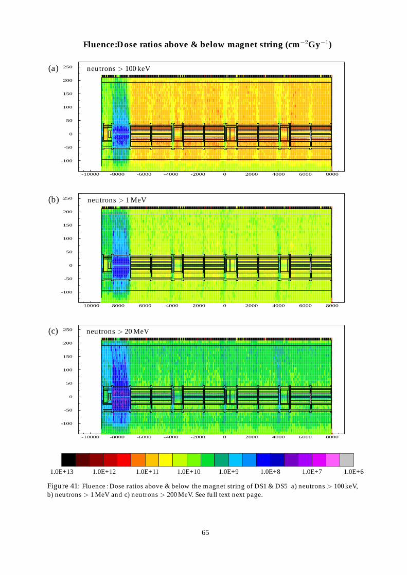
-100

-50

0

50

100

150

200

250

-10000 -8000 -6000 -4000 -2000 0 2000 4000 6000 8000

-100

-50

0

50

100

150

200

250

-10000 -8000 -6000 -4000 -2000 0 2000 4000 6000 8000

-100

-50

0

50

100

150

200

250

-10000 -8000 -6000 -4000 -2000 0 2000 4000 6000 8000

(a) neutrons > 100 keV

(b) neutrons > 1 MeV

(c) neutrons > 20 MeV

1.0E+13 1.0E+12 1.0E+11 1.0E+10 1.0E+9 1.0E+8 1.0E+7 1.0E+6

Fluence:Dose ratios above & below magnet string (cm−2Gy−1)

Figure 41: Fluence : Dose ratios above & below the magnet string of DS1 & DS5 a) neutrons > 100 keV,b) neutrons > 1 MeV and c) neutrons > 200 MeV. See full text next page.

65

-100

-50

0

50

100

150

200

250

-10000 -8000 -6000 -4000 -2000 0 2000 4000 6000 8000

-100

-50

0

50

100

150

200

250

-10000 -8000 -6000 -4000 -2000 0 2000 4000 6000 8000

(c) neutrons > 50 MeV

(d) neutrons > 100 MeV

1.0E+13 1.0E+12 1.0E+11 1.0E+10 1.0E+9 1.0E+8 1.0E+7 1.0E+6

Figure 41: Neutron fluence : dose ratio distributions above and below the magnet string in the dispersion sup-pressors of DS1 & DS5. Values are the same for both dispersion suppressor sections. Absolute values for theannual neutron fluence can be obtained by combining these plots with the corresponding annual dose maps forDS1 (Figure 16) and DS5 (Figure 17). Plots (a)-(e) are shown for various neutron energy cuts: a) neutrons > 100keV (responsible for bulk damage in Si), b) neutrons > 1 MeV, c) neutrons > 20 MeV, d) neutrons > 50 MeV ande) neutrons > 100 MeV. The latter are responsible for SEUs.

66

-100

-50

0

50

100

150

200

250

-10000 -8000 -6000 -4000 -2000 0 2000 4000 6000 8000

-100

-50

0

50

100

150

200

250

-10000 -8000 -6000 -4000 -2000 0 2000 4000 6000 8000

(a) protons > 100 keV

(b) protons > 100 MeV

1.0E+13 1.0E+12 1.0E+11 1.0E+10 1.0E+9 1.0E+8 1.0E+7 1.0E+6

Fluence:Dose ratios above & below magnet string (cm−2Gy−1)

Figure 42: Proton fluence : dose ratio distributions above and below the magnet string in the dispersion suppres-sors of DS1 & DS5. Values are the same for both dispersion suppressor sections. Absolute values for the annualproton fluence can be obtained by combining these plots with the corresponding annual dose maps for DS1 (Fig-ure 16) and DS5 (Figure 17). Plots (a) & (b) are shown for the two energy cuts: a) protons > 100 keV and b) protons> 1 MeV. There is very little difference in the ratio of fluence : dose for protons between these energy cuts.

67

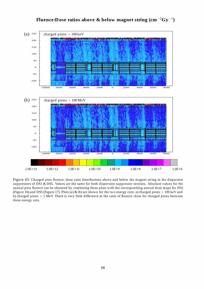
-100

-50

0

50

100

150

200

250

-10000 -8000 -6000 -4000 -2000 0 2000 4000 6000 8000

-100

-50

0

50

100

150

200

250

-10000 -8000 -6000 -4000 -2000 0 2000 4000 6000 8000

(a) charged pions > 100 keV

(b) charged pions > 100 MeV

1.0E+13 1.0E+12 1.0E+11 1.0E+10 1.0E+9 1.0E+8 1.0E+7 1.0E+6

Fluence:Dose ratios above & below magnet string (cm−2Gy−1)

Figure 43: Charged pion fluence : dose ratio distributions above and below the magnet string in the dispersionsuppressors of DS1 & DS5. Values are the same for both dispersion suppressor sections. Absolute values for theannual pion fluence can be obtained by combining these plots with the corresponding annual dose maps for DS1(Figure 16) and DS5 (Figure 17). Plots (a) & (b) are shown for the two energy cuts: a) charged pions > 100 keV andb) charged pions > 1 MeV. There is very little difference in the ratio of fluence : dose for charged pions betweenthese energy cuts.

68

-100

-50

0

50

100

150

200

250

-10000 -8000 -6000 -4000 -2000 0 2000 4000 6000 8000

-100

-50

0

50

100

150

200

250

-10000 -8000 -6000 -4000 -2000 0 2000 4000 6000 8000

-100

-50

0

50

100

150

200

250

-10000 -8000 -6000 -4000 -2000 0 2000 4000 6000 8000

(a) hadrons > 100 keV

(b) hadrons > 1 MeV

(c) hadrons > 20 MeV

1.0E+13 1.0E+12 1.0E+11 1.0E+10 1.0E+9 1.0E+8 1.0E+7 1.0E+6

Fluence:Dose ratios above & below magnet string (cm−2Gy−1)

Figure 44: Fluence : Dose ratios above & below the magnet string of DS1 & DS5 a) hadrons > 100 keV,b) hadrons > 1 MeV and c) hadrons > 200 MeV. See full text next page.

69

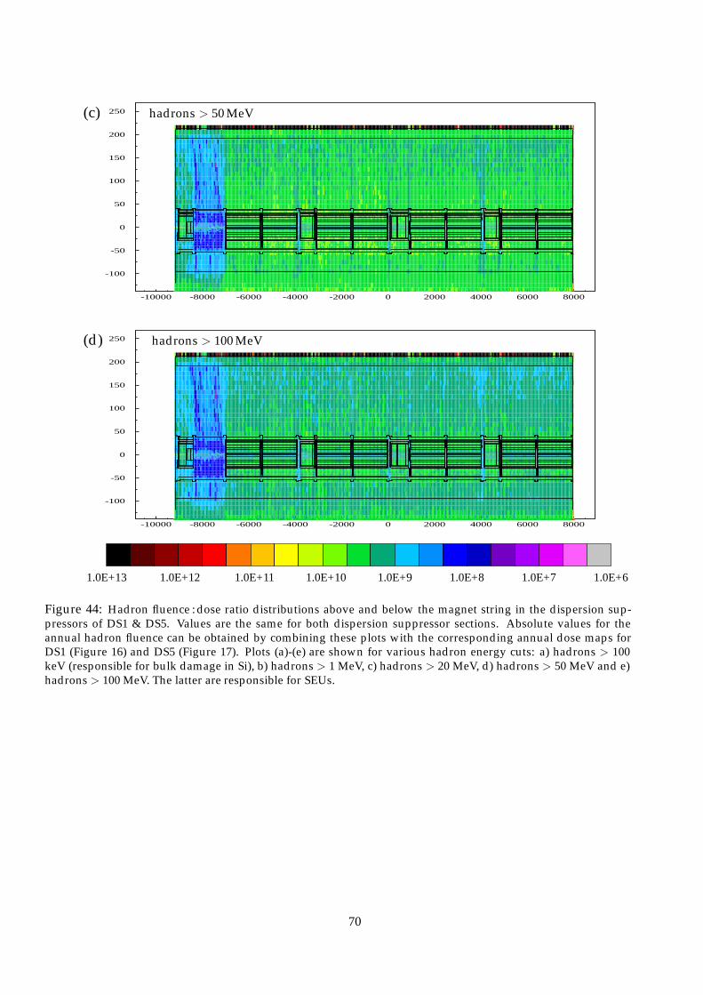
-100

-50

0

50

100

150

200

250

-10000 -8000 -6000 -4000 -2000 0 2000 4000 6000 8000

-100

-50

0

50

100

150

200

250

-10000 -8000 -6000 -4000 -2000 0 2000 4000 6000 8000

(c) hadrons > 50 MeV

(d) hadrons > 100 MeV

1.0E+13 1.0E+12 1.0E+11 1.0E+10 1.0E+9 1.0E+8 1.0E+7 1.0E+6

Figure 44: Hadron fluence : dose ratio distributions above and below the magnet string in the dispersion sup-pressors of DS1 & DS5. Values are the same for both dispersion suppressor sections. Absolute values for theannual hadron fluence can be obtained by combining these plots with the corresponding annual dose maps forDS1 (Figure 16) and DS5 (Figure 17). Plots (a)-(e) are shown for various hadron energy cuts: a) hadrons > 100keV (responsible for bulk damage in Si), b) hadrons > 1 MeV, c) hadrons > 20 MeV, d) hadrons > 50 MeV and e)hadrons > 100 MeV. The latter are responsible for SEUs.

70

Appendix B.2

Radial fluence : dose distributions in the LHC tunnel

71

-200

-100

0

100

200

-200 -100 0 100 200 300

-200

-100

0

100

200

-200 -100 0 100 200 300

-200

-100

0

100

200

-200 -100 0 100 200 300

-200

-100

0

100

200

-200 -100 0 100 200 300

-200

-100

0

100

200

-200 -100 0 100 200 300

1.0E+13 1.0E+12 1.0E+11 1.0E+10 1.0E+9 1.0E+8 1.0E+7 1.0E+6

Neutron Fluence:Dose ratios in LHC tunnel at Q11

a) n > 100 keV b) n > 1 MeV

c) n > 20 MeV d) n > 50 MeV

e) n > 100 MeV

Figure 45: Radial fluence : dose distributions (cm−2Gy−1) in the LHC tunnel for neutrons above vari-ous energy cuts in the vicinity of Q11 for DS1 & DS5.

72

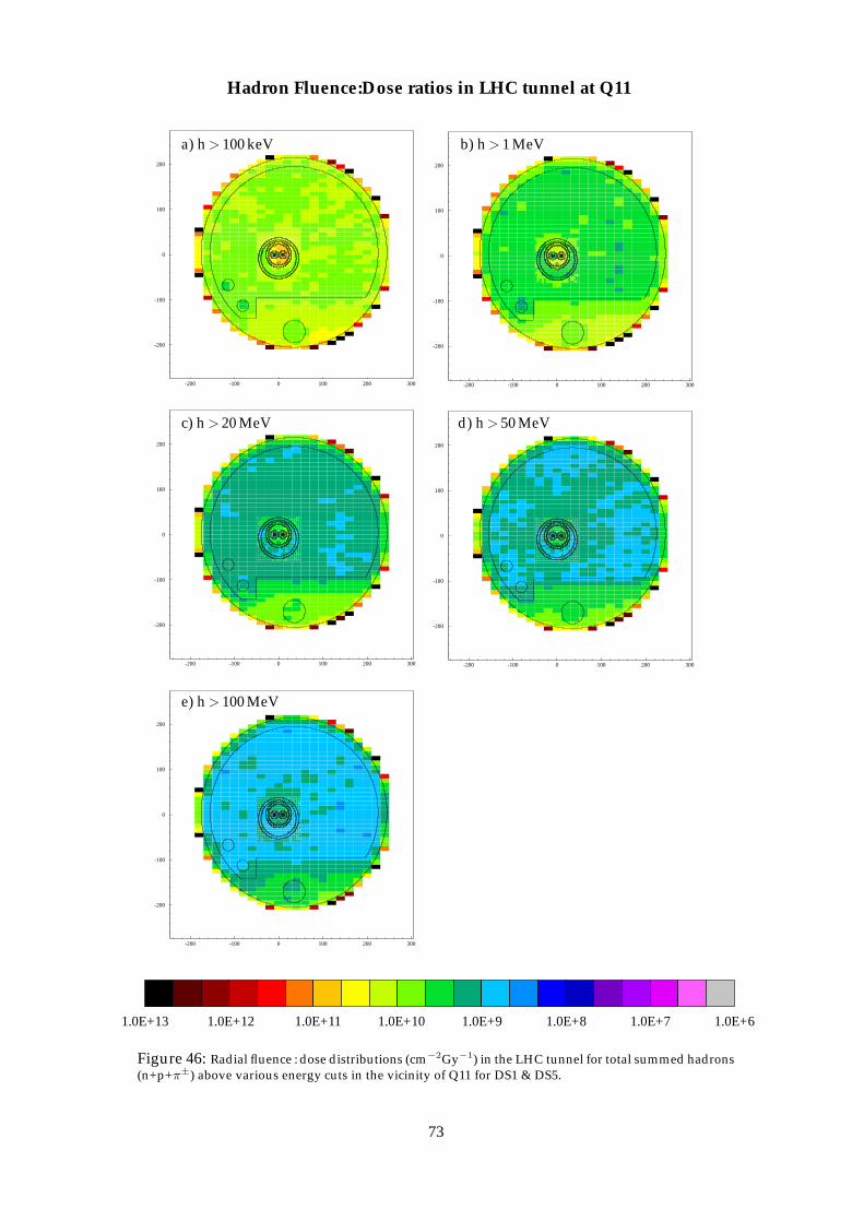
-200

-100

0

100

200

-200 -100 0 100 200 300

-200

-100

0

100

200

-200 -100 0 100 200 300

-200

-100

0

100

200

-200 -100 0 100 200 300

-200

-100

0

100

200

-200 -100 0 100 200 300

-200

-100

0

100

200

-200 -100 0 100 200 300

1.0E+13 1.0E+12 1.0E+11 1.0E+10 1.0E+9 1.0E+8 1.0E+7 1.0E+6

Hadron Fluence:Dose ratios in LHC tunnel at Q11

a) h > 100 keV b) h > 1 MeV

c) h > 20 MeV d) h > 50 MeV

e) h > 100 MeV

Figure 46: Radial fluence : dose distributions (cm−2Gy−1) in the LHC tunnel for total summed hadrons(n+p+π±) above various energy cuts in the vicinity of Q11 for DS1 & DS5.

73

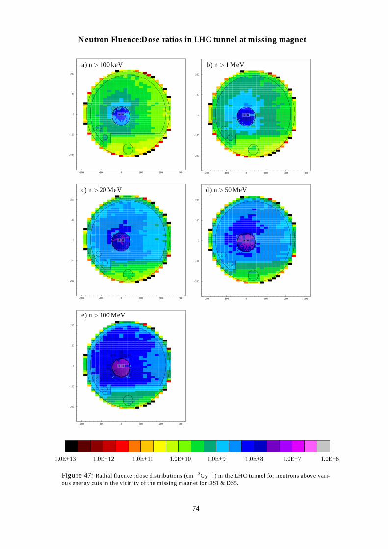
-200

-100

0

100

200

-200 -100 0 100 200 300

-200

-100

0

100

200

-200 -100 0 100 200 300

-200

-100

0

100

200

-200 -100 0 100 200 300

-200

-100

0

100

200

-200 -100 0 100 200 300

-200

-100

0

100

200

-200 -100 0 100 200 300

1.0E+13 1.0E+12 1.0E+11 1.0E+10 1.0E+9 1.0E+8 1.0E+7 1.0E+6

Neutron Fluence:Dose ratios in LHC tunnel at missing magnet

a) n > 100 keV b) n > 1 MeV

c) n > 20 MeV d) n > 50 MeV

e) n > 100 MeV

Figure 47: Radial fluence : dose distributions (cm−2Gy−1) in the LHC tunnel for neutrons above vari-ous energy cuts in the vicinity of the missing magnet for DS1 & DS5.

74

-200

-100

0

100

200

-200 -100 0 100 200 300

-200

-100

0

100

200

-200 -100 0 100 200 300

-200

-100

0

100

200

-200 -100 0 100 200 300

-200

-100

0

100

200

-200 -100 0 100 200 300

-200

-100

0

100

200

-200 -100 0 100 200 300

1.0E+13 1.0E+12 1.0E+11 1.0E+10 1.0E+9 1.0E+8 1.0E+7 1.0E+6

Hadron Fluence:Dose ratios in LHC tunnel at missing magnet

a) h > 100 keV b) h > 1 MeV

c) h > 20 MeV d) h > 50 MeV

e) h > 100 MeV

Figure 48: Radial fluence : dose distributions (cm−2Gy−1) in the LHC tunnel for total summed hadrons(n+p+π±) above various energy cuts in the vicinity of the missing magnet for DS1 & DS5.

75

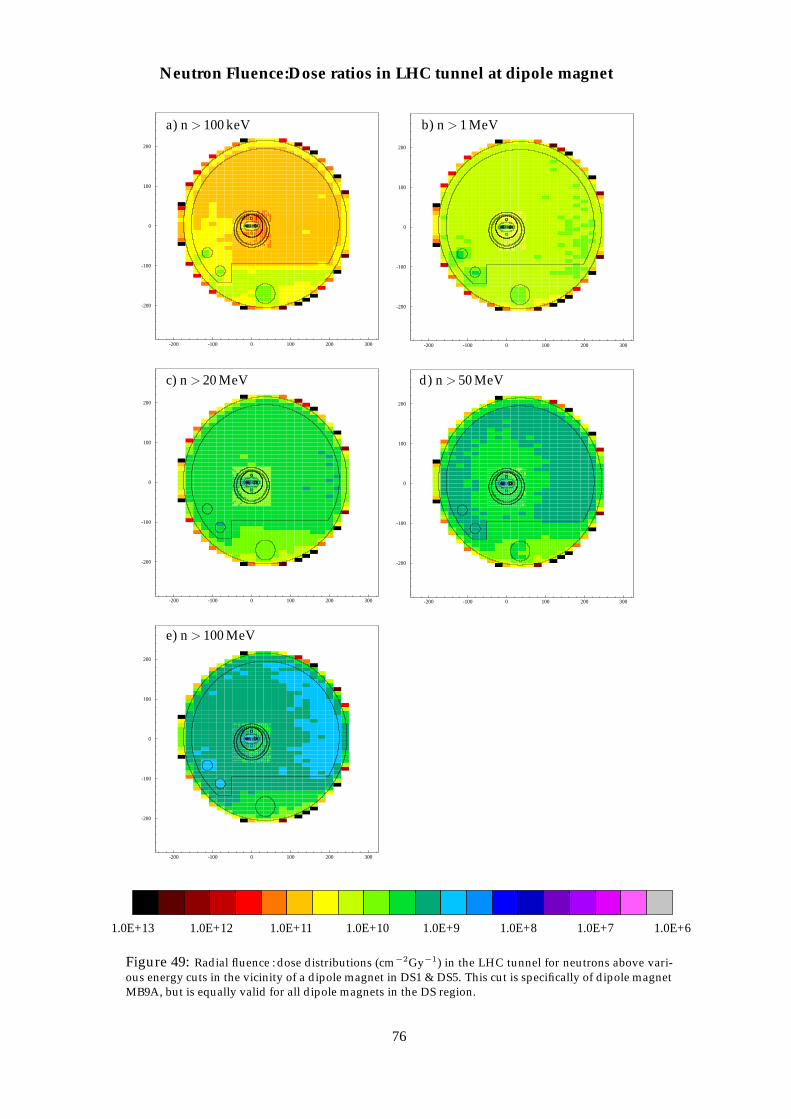
-200

-100

0

100

200

-200 -100 0 100 200 300

-200

-100

0

100

200

-200 -100 0 100 200 300

-200

-100

0

100

200

-200 -100 0 100 200 300

-200

-100

0

100

200

-200 -100 0 100 200 300

-200

-100

0

100

200

-200 -100 0 100 200 300

1.0E+13 1.0E+12 1.0E+11 1.0E+10 1.0E+9 1.0E+8 1.0E+7 1.0E+6

Neutron Fluence:Dose ratios in LHC tunnel at dipole magnet

a) n > 100 keV b) n > 1 MeV

c) n > 20 MeV d) n > 50 MeV

e) n > 100 MeV

Figure 49: Radial fluence : dose distributions (cm−2Gy−1) in the LHC tunnel for neutrons above vari-ous energy cuts in the vicinity of a dipole magnet in DS1 & DS5. This cut is specifically of dipole magnetMB9A, but is equally valid for all dipole magnets in the DS region.

76

-200

-100

0

100

200

-200 -100 0 100 200 300

-200

-100

0

100

200

-200 -100 0 100 200 300

-200

-100

0

100

200

-200 -100 0 100 200 300

-200

-100

0

100

200

-200 -100 0 100 200 300

-200

-100

0

100

200

-200 -100 0 100 200 300

1.0E+13 1.0E+12 1.0E+11 1.0E+10 1.0E+9 1.0E+8 1.0E+7 1.0E+6

Hadron Fluence:Dose ratios in LHC tunnel at dipole magnet

a) h > 100 keV b) h > 1 MeV

c) h > 20 MeV d) h > 50 MeV

e) h > 100 MeV

Figure 50: Radial fluence : dose distributions (cm−2Gy−1) in the LHC tunnel for total summed hadrons(n+p+π±) above various energy cuts in the vicinity of a dipole magnet in DS1 & DS5. This cut is specifi-cally of dipole magnet MB9A, but is equally valid for all dipole magnets in the DS region.

77

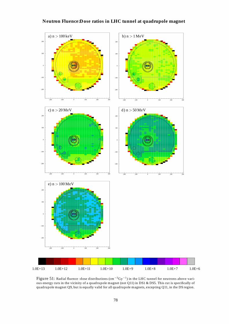
-200

-100

0

100

200

-200 -100 0 100 200 300

-200

-100

0

100

200

-200 -100 0 100 200 300

-200

-100

0

100

200

-200 -100 0 100 200 300

-200

-100

0

100

200

-200 -100 0 100 200 300

-200

-100

0

100

200

-200 -100 0 100 200 300

1.0E+13 1.0E+12 1.0E+11 1.0E+10 1.0E+9 1.0E+8 1.0E+7 1.0E+6

Neutron Fluence:Dose ratios in LHC tunnel at quadrupole magnet

a) n > 100 keV b) n > 1 MeV

c) n > 20 MeV d) n > 50 MeV

e) n > 100 MeV

Figure 51: Radial fluence : dose distributions (cm−2Gy−1) in the LHC tunnel for neutrons above vari-ous energy cuts in the vicinity of a quadrupole magnet (not Q11) in DS1 & DS5. This cut is specifically ofquadrupole magnet Q9, but is equally valid for all quadrupole magnets, excepting Q11, in the DS region.

78

-200

-100

0

100

200

-200 -100 0 100 200 300

-200

-100

0

100

200

-200 -100 0 100 200 300

-200

-100

0

100

200

-200 -100 0 100 200 300

-200

-100

0

100

200

-200 -100 0 100 200 300

-200

-100

0

100

200

-200 -100 0 100 200 300

1.0E+13 1.0E+12 1.0E+11 1.0E+10 1.0E+9 1.0E+8 1.0E+7 1.0E+6

Hadron Fluence:Dose ratios in LHC tunnel at quadrupole magnet

a) h > 100 keV b) h > 1 MeV

c) h > 20 MeV d) h > 50 MeV

e) h > 100 MeV

Figure 52: Radial fluence : dose distributions (cm−2Gy−1) in the LHC tunnel for total summed hadrons(n+p+π±) above various energy cuts in the vicinity of a quadpole magnet (not Q11) in DS1 & DS5. Thiscut is specifically of quadrupole magnet Q9, but is equally valid for all quadrupole magnets, exceptingQ11, in the DS region.

79

-200

-100

0

100

200

-200 -100 0 100 200 300

-200

-100

0

100

200

-200 -100 0 100 200 300

-200

-100

0

100

200

-200 -100 0 100 200 300

-200

-100

0

100

200

-200 -100 0 100 200 300

-200

-100

0

100

200

-200 -100 0 100 200 300

1.0E+13 1.0E+12 1.0E+11 1.0E+10 1.0E+9 1.0E+8 1.0E+7 1.0E+6

Neutron Fluence:Dose ratios in LHC tunnel at intermagnet gap

a) n > 100 keV b) n > 1 MeV

c) n > 20 MeV d) n > 50 MeV

e) n > 100 MeV

Figure 53: Radial fluence : dose distributions (cm−2Gy−1) in the LHC tunnel for neutrons above vari-ous energy cuts in the vicinity of an intermagnet gap (in region MB8B-MB11A) in DS1 & DS5.

80

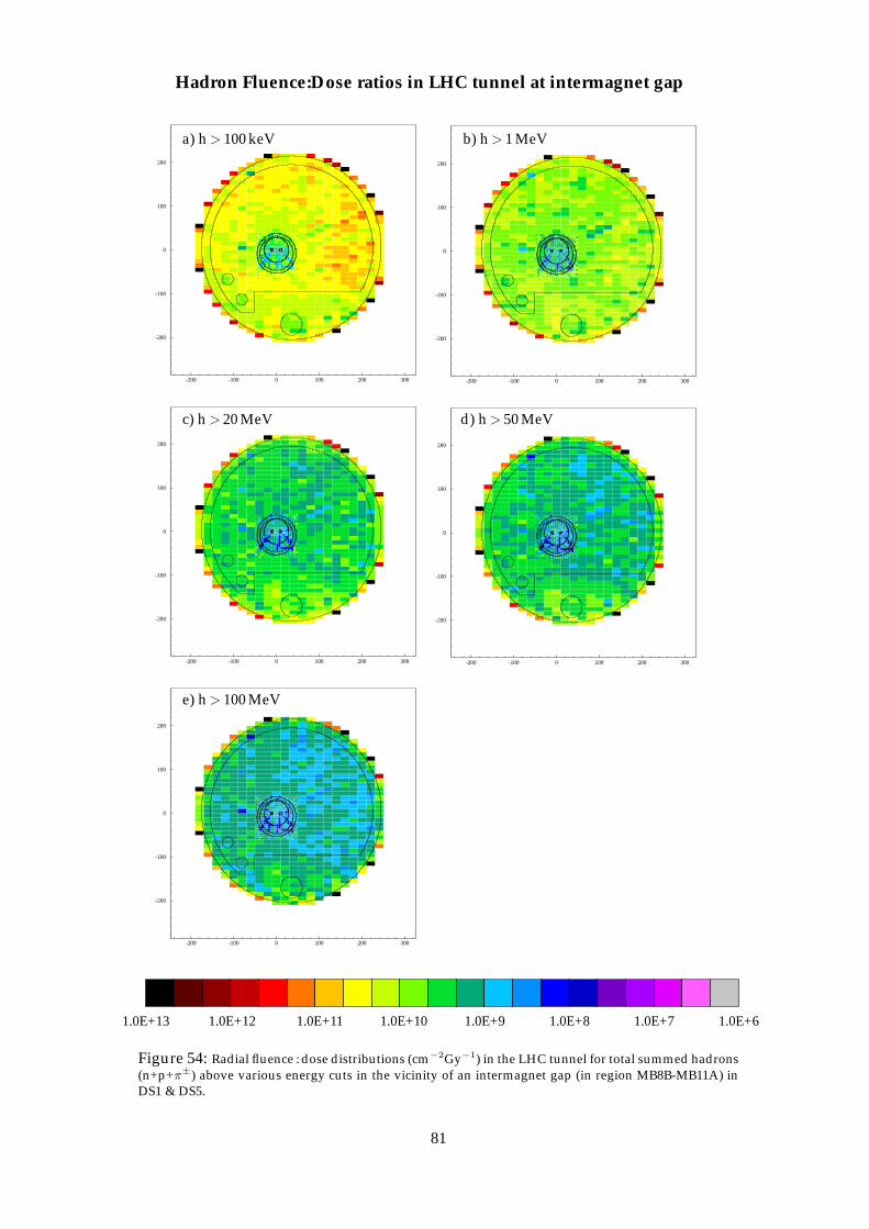
-200

-100

0

100

200

-200 -100 0 100 200 300

-200

-100

0

100

200

-200 -100 0 100 200 300

-200

-100

0

100

200

-200 -100 0 100 200 300

-200

-100

0

100

200

-200 -100 0 100 200 300

-200

-100

0

100

200

-200 -100 0 100 200 300

1.0E+13 1.0E+12 1.0E+11 1.0E+10 1.0E+9 1.0E+8 1.0E+7 1.0E+6

Hadron Fluence:Dose ratios in LHC tunnel at intermagnet gap

a) h > 100 keV b) h > 1 MeV

c) h > 20 MeV d) h > 50 MeV

e) h > 100 MeV

Figure 54: Radial fluence : dose distributions (cm−2Gy−1) in the LHC tunnel for total summed hadrons(n+p+π±) above various energy cuts in the vicinity of an intermagnet gap (in region MB8B-MB11A) inDS1 & DS5.

81

Appendix B.3

Quantitative fluence : dose valuesfor the dispersion suppressors DS1 & DS5

82

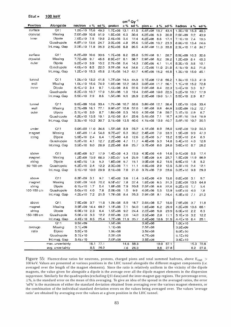
Figure 55: Fluence:dose ratios for neutrons, protons, charged pions and total summed hadrons, above Ecut >100 keV. Values are presented at various positions in the LHC tunnel alongside the different magnet components (i.e.averaged over the length of the magnet elements). Since the ratio is relatively uniform in the vicinity of the dipolemagnets, the value given for alongside a dipole is the average over all the dipole magnet elements in the dispersionsuppressor. Similarly for the quadrupoles (excluding Q11 data) and the inter-magnet gap regions. The percentage error,±%, is the standard error on the mean of this averaging. To give an idea of the spread in the averaged ratios, the error’sd%’ is the maximum of either the standard deviation obtained from averaging over the various magnet elements, orthe combination of the individual standard deviation errors on the values being averaged over. The values ’averageratio’ are obtained by averaging over the values at a given position in the LHC tunnel.

83

Figure 56: Fluence:dose ratios for neutrons, protons, charged pions and total summed hadrons, above Ecut > 1 MeV.Values are presented at various positions in the LHC tunnel alongside the different magnet components (i.e. averagedover the length of the magnet elements). Since the ratio is relatively uniform in the vicinity of the dipole magnets,the value given for alongside a dipole is the average over all the dipole magnet elements in the dispersion suppressor.Similarly for the quadrupoles (excluding Q11 data) and the inter-magnet gap regions. The percentage error, ±%, isthe standard error on the mean of this averaging. To give an idea of the spread in the averaged ratios, the error ’sd%’is the maximum of either the standard deviation obtained from averaging over the various magnet elements, or thecombination of the individual standard deviation errors on the values being averaged over. The values ’average ratio’are obtained by averaging over the values at a given position in the LHC tunnel.

84

Figure 57: Fluence:dose ratios for neutrons, protons, charged pions and total summed hadrons, above Ecut > 20 MeV.Values are presented at various positions in the LHC tunnel alongside the different magnet components (i.e. averagedover the length of the magnet elements). Since the ratio is relatively uniform in the vicinity of the dipole magnets,the value given for alongside a dipole is the average over all the dipole magnet elements in the dispersion suppressor.Similarly for the quadrupoles (excluding Q11 data) and the inter-magnet gap regions. The percentage error, ±%, isthe standard error on the mean of this averaging. To give an idea of the spread in the averaged ratios, the error ’sd%’is the maximum of either the standard deviation obtained from averaging over the various magnet elements, or thecombination of the individual standard deviation errors on the values being averaged over. The values ’average ratio’are obtained by averaging over the values at a given position in the LHC tunnel.

85

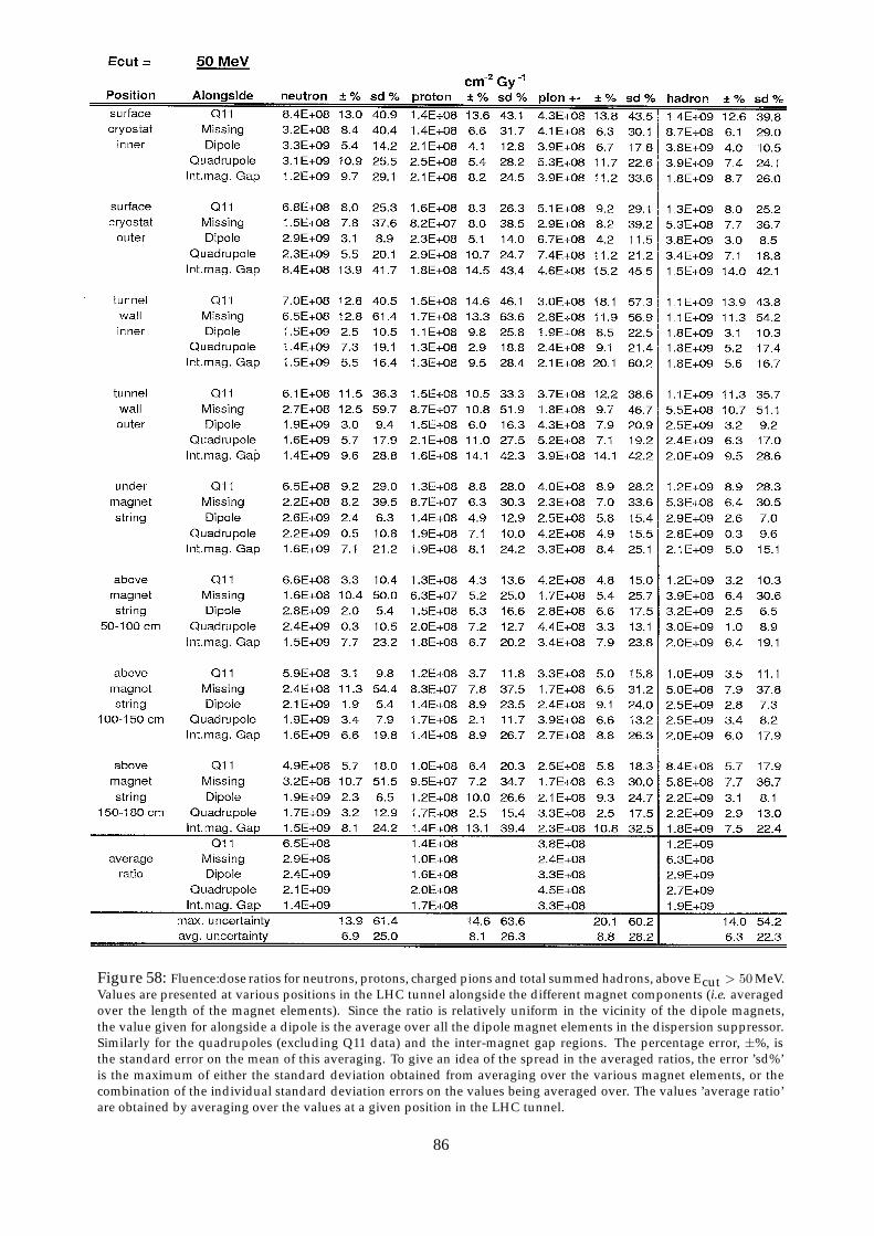
Figure 58: Fluence:dose ratios for neutrons, protons, charged pions and total summed hadrons, above Ecut > 50 MeV.Values are presented at various positions in the LHC tunnel alongside the different magnet components (i.e. averagedover the length of the magnet elements). Since the ratio is relatively uniform in the vicinity of the dipole magnets,the value given for alongside a dipole is the average over all the dipole magnet elements in the dispersion suppressor.Similarly for the quadrupoles (excluding Q11 data) and the inter-magnet gap regions. The percentage error, ±%, isthe standard error on the mean of this averaging. To give an idea of the spread in the averaged ratios, the error ’sd%’is the maximum of either the standard deviation obtained from averaging over the various magnet elements, or thecombination of the individual standard deviation errors on the values being averaged over. The values ’average ratio’are obtained by averaging over the values at a given position in the LHC tunnel.

86

Figure 59: Fluence:dose ratios for neutrons, protons, charged pions and total summed hadrons, above Ecut >100 MeV. Values are presented at various positions in the LHC tunnel alongside the different magnet components(i.e. averaged over the length of the magnet elements). Since the ratio is relatively uniform in the vicinity of the dipolemagnets, the value given for alongside a dipole is the average over all the dipole magnet elements in the dispersionsuppressor. Similarly for the quadrupoles (excluding Q11 data) and the inter-magnet gap regions. The percentage error,±%, is the standard error on the mean of this averaging. To give an idea of the spread in the averaged ratios, the error’sd%’ is the maximum of either the standard deviation obtained from averaging over the various magnet elements, orthe combination of the individual standard deviation errors on the values being averaged over. The values ’averageratio’ are obtained by averaging over the values at a given position in the LHC tunnel.

87