radar remote sensing of arid regions - university of michigan

Radar Remote Sensing of Arid Regions

by

Adel A. Elsherbini

A dissertation submitted in partial fulfillment

of the requirements for the degree of

Doctor of Philosophy

(Electrical Engineering)

in The University of Michigan

2011

Doctoral Committee:

Professor Kamal Sarabandi, Chair

Professor Ronald Gilgenbach

Professor Eric Michielssen

Professor Mahta Moghaddam

ii

To my father and mother with love and gratitude.

iii

ACKNOWLEDGMENTS

Most importantly, I would like to thank my research advisor and mentor, Prof.

Kamal Sarabandi. He offered me the chance to work with him on many interesting and

challenging problems. He is a truly outstanding and inspiring advisor. I cannot count the

times I almost gave up on some of the research problems but he would encourage me to

think on it from a different angle and we end up reaching a solution. I would like also to

thank Prof. Eric Michielssen, Prof. Mahta Moghaddam and Prof. Ronald Gilgenbach for

their service on my dissertation committee.

During my PhD research period at the University of Michigan, I had the

opportunity to interact with many outstanding researchers and to learn a lot from them. In

particular, I would like to thank Dr. Adib Nashashibi for his assistance and advice on

several research and measurements problems. I would like also to thank Pelumi Osoba,

Fikadu Dagefu, Yohan Kim, Dr. Line Van Nieuwstadt, Victor Lee, Danial Ehyaie,

Michael Benson, Dr. Wonbin Hong, Dr. Michael Thiel, Dr. Mojtaba Dehmollaian, Scott

Rudolph, Amit Patel, Mark Haynes, Yuriy Goykhman, Hatim Bukhari, Young Jun, Dr.

Jacquelyn Vitaz, Xueyang Duan, Meysam Moallem, Yong Jun Song, Sangjo Choi, Dr.

Alireza Tabatabaeenejad, Onur Bakir, Jungsuek Oh, Xi Lin, Dr. Juseop Lee, Dr. Josh Fu,

Chris Berry, Mehrnoosh Vahidbpour, Mariko Burgin, Ning Wang and Christine

Tannahill for their continuous help and support and for being not only good research

colleagues but also good friends.

iv

I wouldn’t have reached this stage without the support and encouragement of

many of my research colleagues and friends from my previous schools. In particular, I

would like to thank my previous advisors, Prof. Alaa Kamel, Prof. Aly Fathy, Prof.

Abbas Omar and Prof. Hadia Elhennawy and my uncle, Prof. Moniem Elsherbiny. They

encouraged me to work in the field of electromagnetics and they taught me the basics and

ethics of doing research. I would like also to thank my research colleagues and friends,

Dr. Song Lin, Dr. Ahmed Boutejdar, Dr. Songnan Yang, Dr. Cemin (Alex) Zhang, Dr.

Chunna Zhang, Dr. Mohammed Awida, George Isaac, Amr Elshazly, Dr. Telesphor

Kamgaing, Dr. Henning Braunisch, Dr. Krishna Bharath, Amr Ali and Amr Amin.

Adel A. Elsherbini

April 29, 2011

v

Table of Contents

DEDICATION ................................................................................................................... iii

ACKNOWLEDGMENTS ................................................................................................. iii

LIST OF FIGURES .............................................................................................................x

LIST OF TABLES ......................................................................................................... xxiii

Introduction ......................................................................................................1 Chapter 1

1.1 Motivation ........................................................................................................... 1

1.2 Applications ........................................................................................................ 2

1.2.1 Oil Fields and Ground Water Explorations .................................................... 2

1.2.2 Mine Field Detection ...................................................................................... 3

1.2.3 Other Applications .......................................................................................... 5

1.3 Approach ............................................................................................................. 6

1.4 Thesis Framework ............................................................................................... 9

Subsurface InSAR Design .............................................................................13 Chapter 2

2.1 Conventional Interferometric SAR (InSAR) .................................................... 13

2.2 Extension of InSAR for Subsurface Mapping .................................................. 15

2.2.1 Sample Scenario............................................................................................ 15

2.2.2 Proposed System ........................................................................................... 16

2.3 Scattering Phenomena ....................................................................................... 17

2.4 Subsurface InSAR Processing .......................................................................... 22

vi

2.4.1 Subsurface Focusing ..................................................................................... 23

2.4.2 Image Coregistration ..................................................................................... 24

2.5 Left/Right Separation ........................................................................................ 27

2.6 Conclusion ........................................................................................................ 30

Subsurface Topography Inversion Algorithm ...............................................32 Chapter 3

3.1 Subsurface Propagation Modeling .................................................................... 32

3.2 Inversion Algorithm .......................................................................................... 34

3.3 Sensitivity Analysis of the Height Estimation .................................................. 39

3.4 Experimental Results ........................................................................................ 44

3.5 Conclusion ........................................................................................................ 48

Image Distortion Effects in SAR Subsurface Imaging and a New Iterative Chapter 4

Approach for Refocusing and Coregistration .............................................................50

4.1 Fast Subsurface SAR Simulator & Subsurface Focusing Technique ............... 51

4.2 Defocusing and Distortion Effects in SAR Subsurface Imaging ...................... 56

4.2.1 Defocusing Effects ........................................................................................ 56

4.2.2 Geometric Distortion Effects ........................................................................ 58

4.2.3 Caustic Surfaces and their Effects ................................................................ 61

4.3 Iterative Approach ............................................................................................ 66

4.4 Simulation Results ............................................................................................ 67

4.5 Scaled Model Measurement Results ................................................................. 71

4.6 Conclusion ........................................................................................................ 72

Linearly Polarized Ultra-Wideband Antennas ...............................................74 Chapter 5

5.1 Background ....................................................................................................... 75

vii

5.1.1 Definitions..................................................................................................... 75

5.1.2 Design Issues ................................................................................................ 75

5.1.3 Common Structures ...................................................................................... 78

5.1.4 Omni-Directional Coupled Sectorial Loop Antenna (CSLA) ...................... 78

5.2 Folded CSLA .................................................................................................... 82

5.2.1 Folded CSLA with Vivaldi Antenna............................................................. 85

5.2.2 Reflector Design for UWB Operation .......................................................... 87

5.2.3 Vivaldi-CSLA Antenna with Reflector ........................................................ 89

5.3 Rectangular Waveguide UWB Antennas.......................................................... 96

5.3.1 Introduction ................................................................................................... 96

5.3.2 Antenna Structure and Operation.................................................................. 97

5.3.3 Design Process .............................................................................................. 99

5.3.4 Feed design ................................................................................................. 102

5.3.5 Measurement Results .................................................................................. 104

5.4 Conclusion ...................................................................................................... 107

High Isolation T/R UWB Antenna Pair .......................................................108 Chapter 6

6.1 Introduction and Motivation ........................................................................... 108

6.2 Antenna Structure and Operation.................................................................... 112

6.3 Parametric Study ............................................................................................. 114

6.3.1 Cavity Fins .................................................................................................. 115

6.3.2 Sectorial Loop Angle .................................................................................. 116

6.3.3 The Cavity Height ....................................................................................... 117

6.3.4 Antenna Separation ..................................................................................... 118

viii

6.3.5 Tapered Feed Line ...................................................................................... 119

6.4 Measurement Results ...................................................................................... 121

6.4.1 Input Impedance and Pattern Measurements .............................................. 121

6.5 Comparison to other structures ....................................................................... 124

6.6 Conclusion ...................................................................................................... 126

Dual Polarized UWB Antennas ...................................................................127 Chapter 7

7.1 Dual Polarized Directional Cavity Backed CSLA .......................................... 127

7.1.1 Antenna Structure ....................................................................................... 127

7.1.2 Parametric Study ......................................................................................... 129

7.2 Diversity Omni-Directional CSLA ................................................................. 133

7.2.1 Antenna Structure ....................................................................................... 133


7.3 Directional Cavity Backed Dual-Polarized CSLA ......................................... 138

7.3.1 Antenna Structure and Principle of Operation ............................................ 138


7.3.3 Actual Feeding Structure ............................................................................ 144


7.4 Conclusion ...................................................................................................... 150

Very Low Profile UWB Antennas ...............................................................151 Chapter 8

8.1 Very Low Profile UWB Monopole................................................................. 151

8.1.1 Introduction ................................................................................................. 151

8.1.2 Antenna Structure and Operation................................................................ 153


ix

8.1.4 Measurements Results ................................................................................ 160

8.2 Very Low Profile Directive Antenna .............................................................. 162

8.2.1 Antenna Structure and Operation................................................................ 163



8.2.4 Improving the Cross-Pol Components ........................................................ 171

8.3 Conclusion ...................................................................................................... 173

Conclusion and Future Work .......................................................................176 Chapter 9

9.1 Conclusions ..................................................................................................... 176

9.1.1 Scattering Phenomena ................................................................................. 176

9.1.2 Subsurface Processing ................................................................................ 177

9.1.3 Inversion Algorithm .................................................................................... 177

9.1.4 Image Correction Algorithm ....................................................................... 178

9.1.5 Compact UWB Antennas ............................................................................ 178

9.1.6 Linearly Polarized UWB Antennas ............................................................ 179

9.1.7 High Isolation Antenna Pair ........................................................................ 180

9.1.8 Dual Polarized Antennas............................................................................. 181

9.1.9 Very Low-Profile Antennas ........................................................................ 181

9.2 Future Work .................................................................................................... 182

9.2.1 Scattering from Targets under a Rough Surface ......................................... 182

9.2.2 Scattering from Large Dunes ...................................................................... 182

9.2.3 Scattering and Propagation in Dense Random Media ................................ 183

Bibliography ....................................................................................................................184

x

LIST OF FIGURES

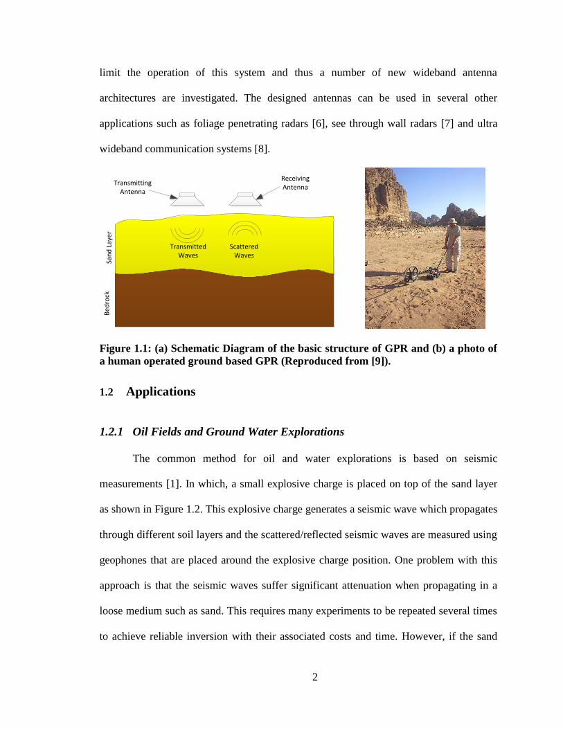
Figure 1.1: (a) Schematic Diagram of the basic structure of GPR and (b) a photo of a

human operated ground based GPR (Reproduced from [9]). ..................................... 2

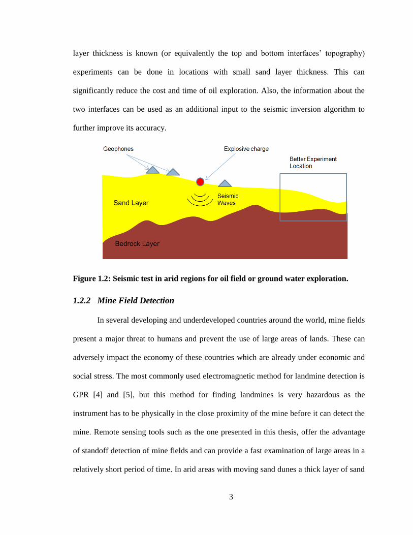
Figure 1.2: Seismic test in arid regions for oil field or ground water exploration. ............. 3

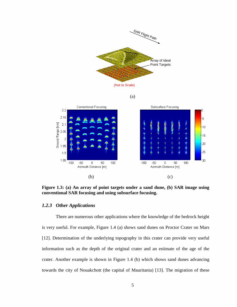
Figure 1.3: (a) An array of point targets under a sand dune, (b) SAR image using

conventional SAR focusing and using subsurface focusing. ...................................... 5

Figure 1.4: (a) Sand dunes in Proctor Crater on Mars [12] and (b) Sand dunes advancing

towards the city of Nouakchott (the capital of Mauritania) [13]. ............................... 6

Figure 1.5: Conventional remote sensing techniques for terrain mapping [14]. ................ 7

Figure 1.6: The proposed dual frequency InSAR systems, Ka-InSAR provides top surface

height information that are then used to correct the VHF InSAR data to obtain the

correct subsurface height. ........................................................................................... 8

Figure 1.7: The Different Aspects of the Problem of Radar Remote Sensing of Arid

Regions. .................................................................................................................... 10

Figure 2.1: Steps for generating the terrain height using InSAR. ..................................... 14

Figure 2.2: Using conventional InSAR phase-to-height equations results in severe errors

in the estimated bedrock height. ............................................................................... 16

Figure 2.3: (a) Wave propagation path for the Ka-InSAR (high frequency) and (b) wave

propagation path for VHF-InSAR (low frequency). ................................................. 17

xi

Figure 2.4: Arid areas considered (in Saudi Arabia). The two figures on the left show the

large scale undulations (with a person standing next to a sand dune in the leftmost

photo for comparison) whereas the figure to the right shows the small scale

undulations. ............................................................................................................... 18

Figure 2.5: Promoted scattering mechanisms. .................................................................. 19

Figure 2.6: Simulated backscattering cross-section for the bedrock and sand surfaces

using the parameters in Table 2.2. The decrease in the bedrock backscattering at

higher frequencies is due to the attenuation through the sand. ................................. 21

Figure 2.7: Numerically calculated backscattering coefficient of the c50-70 sand layer as

a function of radar frequency. The sand layer was assumed 0.15 m thick, has 0.6 in

volume fraction (from [36]). ..................................................................................... 22

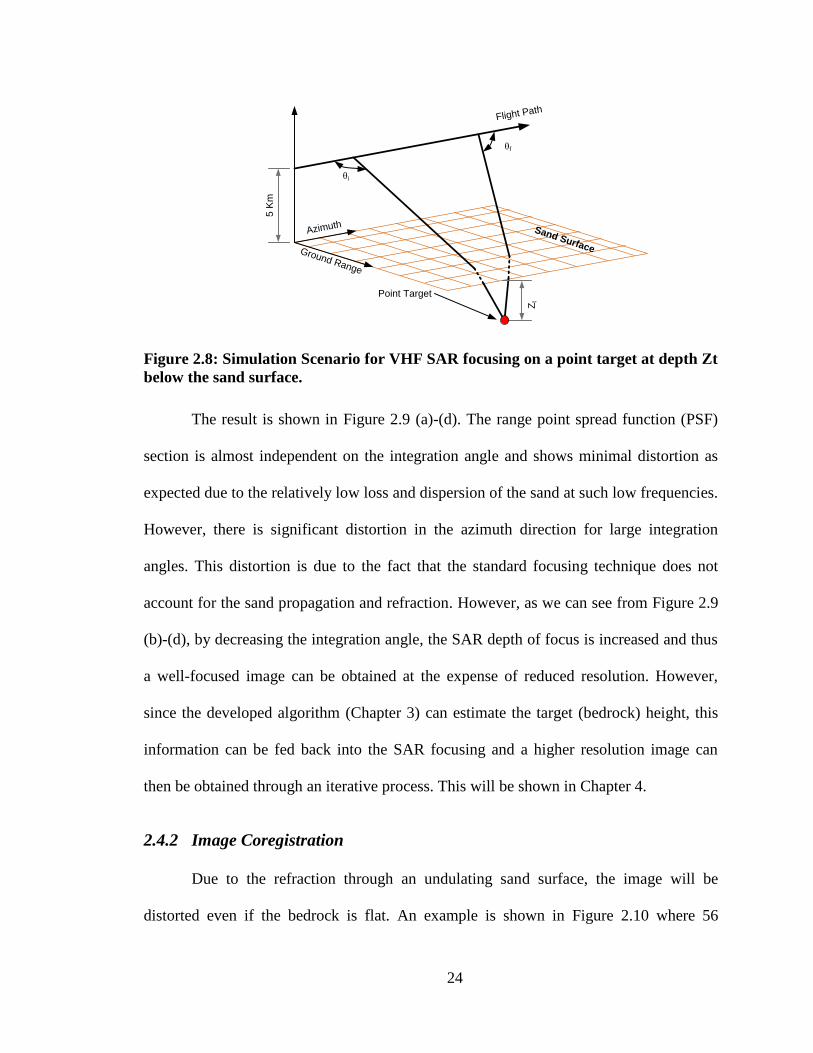
Figure 2.8: Simulation Scenario for VHF SAR focusing on a point target at depth Zt

below the sand surface. ............................................................................................. 24

Figure 2.9: (a) PSF range section, (b) PSF azimuth section for 20o integration angle, (c)

PSF azimuth section for 15o integration angle and (d) PSF azimuth section for 10o

integration angle. ....................................................................................................... 26

Figure 2.10: Image distortion due to top surface undulations (a) geometry and (b) focused

SAR image. ............................................................................................................... 26

Figure 2.11: (a) The antenna pattern for conventional SAR operation and (b) for the

VHF-SAR showing that the undesired targets on the other side of the plane are no

longer suppressed by the antenna radiation pattern. ................................................. 27

Figure 2.12: Left/right separation diagram. ...................................................................... 28

Figure 2.13: Fourier transform of the interferogram. ....................................................... 29

xii

Figure 2.14: The RMS phase error after using two step filters to separate the left and right

components for flat topography vs. the baseline for different operating bandwidths.

................................................................................................................................... 30

Figure 3.1: Geometrical optics modeling for subsurface imaging VHF InSAR (not to

scale for clarity). ....................................................................................................... 33

Figure 3.2: Flow chart of the proposed iterative algorithm for estimating the sand height

above the underlying bedrock. .................................................................................. 34

Figure 3.3: Illustration of the iterative algorithm.............................................................. 37

Figure 3.4: Examples of the results of the iterative algorithm to some sand geometries, (a)

Gaussian shaped dune on top of inverse Gaussian shaped bedrock and (b) linear sand

dunes on top of flat sloped bedrock. ......................................................................... 38

Figure 3.5: Sensitivity of height estimation to sand dielectric constant. .......................... 40

Figure 3.6: Sensitivity of height estimation to interferogram phase accuracy. ................ 41

Figure 3.7: Relative sand thickness errors due to finite range accuracy. .......................... 42

Figure 3.8: Bedrock height errors due to (a) errors in sand height estimation and (b) errors

in sand slope estimation. ........................................................................................... 43

Figure 3.9: Scaled model for verification of the inversion algorithm, (a) schematic and (b)

photo of the actual system. ........................................................................................ 44

Figure 3.10: Experiment scenario, flat sand on top of horizontal bedrock. (a) A photo of

the scene (the sand layer thickness is 7.8cm and the radar movement is along the

horizontal direction), (b) the two SAR images for the two paths (x corresponds to the

azimuth direction) ..................................................................................................... 47

xiii

Figure 3.11: Scaled Model Results: (a) The averaged interforogram (4x4 boxcar

averaging), (b) the unwrapped interferogram, (c) the estimated heights using the

conventional InSAR and (d) the estimated heights using the proposed algorithm. .. 48

Figure 4.1: 3D SAR Geometry. ........................................................................................ 52

Figure 4.2: Interpolation over a non-uniform grid to obtain the target range history. The

contour represents the electrical range to the radar position. The actual grid points

and sand surface are 3D, but the 2D case is plotted for clarity. ................................ 55

Figure 4.3: Azimuth Point Spread Function (APSF) of a point target vs. the target depth

when using conventional focusing with focusing plane at the surface with (a) 20o

integration angle and (b) 40o integration angle, (c) and (d) same scenarios as (a) and

(b) but the target is assumed in air. ........................................................................... 58

Figure 4.4: Sample scenario to illustrate geometric distortion in subsurface SAR images

due to top layer propagation effects, (a) the simulation scenario and (b) the

conventionally focused SAR image. ......................................................................... 60

Figure 4.5: (a) The barchan sand dune, (b) side view and (c) top view of the estimated

caustic surface with the sand dune. The dotted arrows in (c) show the caustic

surfaces corresponding to each curved feature on the sand dune. The radar position

is at (0, 0, 5 km). ....................................................................................................... 63

Figure 4.6: (a) A target at (0, 2025, -60) enclosed within a simple caustic surface

appearing at three different ranges and (b) the simulated range history of the target

using the extended interpolation technique. .............................................................. 65

Figure 4.7: The proposed iterative scheme. ...................................................................... 67

xiv

Figure 4.8: Results of applying the subsurface focusing algorithm: (a) scene consisting of

a linear sand dune and a grid of point targets, (b) the improvement in coherence vs.

different iterations, (c) normalized image from conventional focusing with 10o

integration angle, (d) normalized image from conventional focusing with 40o

integration angle, (e) first iteration of the subsurface focusing algorithm and (f) 3rd

iteration with 40o integration angle. .......................................................................... 69

Figure 4.9: Results of applying the subsurface focusing algorithm: (a) scene consisting of

a barchan sand dune and a grid of point targets, (b) the improvement in coherence

vs. different iterations, (c) normalized image from conventional focusing with 10o

integration angle, (d) normalized image from conventional focusing with 40o

integration angle, (e) first iteration of the subsurface focusing algorithm and (f) 3rd

iteration with 40o integration angle. .......................................................................... 70

Figure 4.10: (a) Conventionally focused SAR image of the scaled model and (b)

comparison between the two coherence histograms obtained. ................................. 72

Figure 5.1: Some Conventional UWB Antennas .............................................................. 78

Figure 5.2: The CSLA Antenna Structure. ....................................................................... 79

Figure 5.3: (a) the fabricated CSLA and (b) its simulated and measured VSWR. ........... 80

Figure 5.4: The normalized radiation pattern of the CSLA antenna in the (a) H-plane and

(b) E-plane. (Solid line is the copolar component and the dashed line is the

crosspolar conponent) ............................................................................................... 80

Figure 5.5: Fully planar CSLA: (a) Structure and (b) simulated VSWR. ......................... 81

Figure 5.6: The magnetic field distribution of the CSLA on the ground plane at 0.5 GHz

(a) isometric view and (b) top view. ......................................................................... 82

xv

Figure 5.7: The structure of the folded CSLA and its simulated VSWR for different

folding angles, β. ....................................................................................................... 83

Figure 5.8: The normalized H-plane radiation pattern of the Folded CSLA antenna for a

folding angle of (a) 135o and (b) 45

o. (Solid line is the copolar component and the

dashed line is the crosspolar conponent)................................................................... 83

Figure 5.9: (a) The Folded CSLA antenna and (b) it simulation and measurment results.

................................................................................................................................... 84

Figure 5.10: A fully planar folded CSLA (a) the structure and (b) the simulation results.

................................................................................................................................... 85

Figure 5.11: (a) The combined Folded CSLA and the Vivaldi Antenna, (b) comparison

between the simulated directivity of the two antennas and (c) the H-plane radiation

pattern of the combined antenna at different frequencies. ........................................ 86

Figure 5.12: (a) The structure of the Vivaldi-CSLA antenna and (b) its simulated and

measured VSWR. ...................................................................................................... 87

Figure 5.13: (a) A dipole parallel to a flat ground plane and (b) the resulting H-plane

radiation pattern for different reflector spacings. ..................................................... 89

Figure 5.14: (a) The Vivaldi-CSLA placed in front of a flat reflector and the simulated (b)

peak directivity of the Vivaldi-CSLA with a planar reflector and (c) the VSWR for

different reflector spacing, d. .................................................................................... 90

Figure 5.15: (a) The Vivaldi-CSLA with the corner reflector, (b) the dimensions of the

CSLA part and (c) the dimensions of the Vivaldi part. ............................................ 91

Figure 5.16: Simulated (a) VSWR and (b) antenna gain for different values of β. .......... 92

Figure 5.17: Simulated (a) VSWR and (b) gain for different values of d. ....................... 93

xvi

Figure 5.18: Measured and simulated input VSWR and gain of the directive CSLA. ..... 94

Figure 5.19. Measured radiation pattern over the operating frequency band: (a) H-plane

and (b) E-plane. ......................................................................................................... 94

Figure 5.20: Time Domain Response. .............................................................................. 96

Figure 5.21: Comparison between the dimensions of a standard ridged horn and the

dimensions of the proposed antenna. λmax is the wavelength at the minimum

operating frequency................................................................................................... 96

Figure 5.22: The proposed structure (a) isometric view and (b) front view. .................... 98

Figure 5.23: Field distribution at the waveguide aperture at 2.4 GHz using (a) the

proposed feed and (b) probe feed (red: highest intensity, blue: zero intensity). ....... 99

Figure 5.24: Simulation results for (a) the effect of the top slot width h1 and (b) the effect

of the shorting line position on the antenna matching. ........................................... 101

Figure 5.25: Current Distribution on the feeding structure at 2.95 GHz. ....................... 102

Figure 5.26: The used balun for feeding the bowtie fed RWGA: (a) A cross section of the

RWGA at its electrical symmetry plane to show the feeding structure and (b) the

balun dimensions. ................................................................................................... 103

Figure 5.27: Photo of the proposed antenna next to a ridged horn antenna operating from

the same minimum frequency. ................................................................................ 104

Figure 5.28: (a) The measured and simulated VSWR of the proposed antenna and (b) the

measured and simulated gain compared to the gain of the ridged horn and that of an

ideal TE10 aperture. ................................................................................................. 105

Figure 5.29: The measured and simulated radiation pattern of the antenna at different

frequencies (a) E-Plane and (b) H-Plane................................................................. 106

xvii

Figure 5.30: Time domain response measurements for the proposed antenna compared to

ridged horn. ............................................................................................................. 107

Figure 6.1: Single antenna and dual antenna radar systems. .......................................... 109

Figure 6.2: Standard methods for increasing the isolation between two antennas (a)

increasing the physical separation, (b) use of lossy elements [53] and (c) use of

isolating elements. ................................................................................................... 111

Figure 6.3: Proposed Antenna structure (a) isometric view and (b) top view. ............... 113

Figure 6.4: The first step for reaching the T/R pair (a) the original dipole version of the

CSLA, (b) the cavity backed CSLA and (c) The VSWR of the two antennas showing

singificant increase in the minimum operating frequency and in-band resonances.

................................................................................................................................. 113

Figure 6.5: The second and third step for reaching the T/R pair (a) adding the annular

slots to decrease the minimum operating frequency for the same antenna size, (b)

adding the fins to remove the in-band resonances, (c) input matching before and

after adding the annular slots and (d) input and output matching before and after

adding the fins. ........................................................................................................ 114

Figure 6.6: (a) Electric field distribution inside the cavity at 2 GHz with the cavity

resonance field component encircled and (b) the effect of the fin height near the

cavity edge on the antenna input matching. ............................................................ 116

Figure 6.7: (a) The input matching and (b) isolation between the two antennas as a

function of the sectorial loop angle, α. .................................................................... 117


function of the cavity height, hcyl. ........................................................................... 118

xviii


function of the antenna separation, Wsep. ................................................................ 119

Figure 6.10: (a) The input impedance at one antenna port when the other port is matched

and (b) the input VSWR as a function of the tapered microstrip line end width. ... 120

Figure 6.11: (a) The fabricated antenna pair and the measured and simulated (b) input

VSWR and (c) isolation. ......................................................................................... 122

Figure 6.12: Measured (solid line) and simulated (dashed line) single element radiation

patterns at the center frequency (1.5 GHz) in the (a) H-plane and (b) E-plane. ..... 123

Figure 6.13: Time domain responses for (a) single antenna, (b) transmit receive antenna

pair and (c) enlarged view of the S21 response overlaid over the ideal sinc pulse. 124

Figure 6.14: Size comparison between the proposed antenna pair and ridged horn antenna

pair ((a) and (b)) and a directive folded CSLA pair ((c) and (d)). .......................... 125

Figure 7.1: (a) Dual-polarized cavity-backed CSLA structure (cavity walls transparent for

clarity) and (b) side view along one of the polarization planes. (The antenna is not

drawn with the correct dimensions to clarify some of the dimensions.)................. 129

Figure 7.2: Effect of the sectorial loop angle, α, on (a) the input matching and (b) the H-

plane radiation pattern at 1.75 GHz. ....................................................................... 131

Figure 7.3: Effect of the cavity height, hc1, on the antenna (a) input matching and (b) E-

plane radiation pattern at 1.7 GHz. ......................................................................... 132

Figure 7.4: Effect of the cavity sidewall heights on (a) the H-plane radiation pattern at

1.75 GHz and (b) the input matching. ..................................................................... 133

Figure 7.5: Diversity CSLA (a) 3D structure and (b) planar structure. .......................... 134

xix

Figure 7.6: Current distribution on the antenna for the two polarizations: (a) horizontal

and (b) vertical. ....................................................................................................... 135

Figure 7.7: Illustration of the reuse of the same V shaped loops for the two polarizations:

(a) horizontal and (b) vertical.................................................................................. 136

Figure 7.8: Effect of the sectorial loop angle on the matching. ...................................... 136

Figure 7.9: (a) Structure of the fabricated diversity antenna and (b) enlarged view of the

feed region (darker yellow traces are on the bottom layer). ................................... 137

Figure 7.10: Input VSWR and isolation of the antenna. ................................................. 137

Figure 7.11: Measured (a) E-plane and (b) H-plane patterns and simulated (c) E-plane

and (d) H-plane patterns. ......................................................................................... 138

Figure 7.12: Antenna structure (a) isometric view and (b) top view showing the ideal

feeding structure. ..................................................................................................... 139

Figure 7.13: (a) and (c) the current distribution on the exciting element and (c), (d) the

electric field distribution inside the cavity at 1.5 GHz for both the vertical and

horizontal excitation modes. ................................................................................... 140

Figure 7.14: The dependence of (a) the MA-VSWR, (b) E-plane and (c) H-plane

directivity at 2 GHz on the cavity height, hc. .......................................................... 142

Figure 7.15: Effect of the bowtie angle on the (a) MA-VSWR and (b) the required

characteristic impedance of the feed line for optimum VSWR. ............................. 143

Figure 7.16: The effect of the feed element width on (a) the MA-VSWR and (b) the E-

plane and (c) H-plane radiation patterns. ................................................................ 145

Figure 7.17: The actual feeding structure using multi-section microstrip line, (a) isometric

view and (b) top view of the exciting element. ....................................................... 147

xx

Figure 7.18: (a) The current distribution on the exciting element and (b) the electric field

distribution inside the cavity at 1.5GHz when using the MS line feed. .................. 147

Figure 7.19: Measured and simulated radiation patterns in the (a), (b) E-plane and (c), (d)

H-plane of the antenna. ........................................................................................... 149

Figure 7.20: (a) Measured and simulated VSWR and (b) measured and simulated S21. 149

Figure 8.1: (a) Initial PCB compatible monopole and (b) the monopole with the inductive

pins. The top circular plate is semi-transparent to show the feed structure. The two

antennas are simulated on an infinite ground plane and fed using and SMA coaxial

cable at the apex. ..................................................................................................... 154

Figure 8.2: The (a) real and (b) imaginary parts of the input impedance of the different

structures. ................................................................................................................ 154

Figure 8.3: Antenna Structure (a) Isometric view and (b) side view with dimensions (the

substrate is not shown for clarity). .......................................................................... 155

Figure 8.4: Current distribution on the antenna feed at different frequencies. ............... 156

Figure 8.5: The effect of the inductive pins width on the (a) input VSWR and (b) the real

part of the input impedance. .................................................................................... 157

Figure 8.6: The effect of the monopole height on the (a) input VSWR and (b) the real part

of the input impedance. ........................................................................................... 158

Figure 8.7: Effect of the feed apex height on (a) the input VSWR and (b) the real and (c)

the imaginary parts of the input impedance. ........................................................... 159

Figure 8.8: Effect of the ground plane size, lg, on the input matching. .......................... 160

Figure 8.9: Effect of the ground plane size on the E-plane pattern at (a) 1 GHz and (b) 2

GHz. ........................................................................................................................ 160

xxi

Figure 8.10: (a) The fabricated antenna and (b) the measured and simulated input VSWR.

................................................................................................................................. 161

Figure 8.11: Measured (a) E-plane and (b) H-plane and simulated (c) E-plane and (H-

plane). ...................................................................................................................... 162

Figure 8.12: (a) Short TEM horn dimensions, (b) its radiation patterns in the E- and H-

planes and (c) its input impedance. ......................................................................... 164

Figure 8.13: (a) Shorted TEM horn structure, (b) effect of the shorting trace width on the

E-plane radiation pattern and on the (c) real and (d) imaginary parts of the input

impedance. .............................................................................................................. 165

Figure 8.14: Antenna structure and dimensions (a) isometric view (ground not shown for

clarity) and (b) side view. ....................................................................................... 166

Figure 8.15: The effect of the antenna length, l, on the (a) input VSWR and (b) the

boresight directivity. ............................................................................................... 167

Figure 8.16: Effect of the antenna length on (a) the input VSWR and (b) the real and (c)

the imaginary component of the input impedance. ................................................. 168

Figure 8.17: Effect of the antenna height on the antenna's (a) input VSWR and (b) real

and (c) imaginary components of the input impedance. ......................................... 169

Figure 8.18: (a) A photo of the fabricated antenna and (b) the measured and the simulated

input VSWR. ........................................................................................................... 170

Figure 8.19: (a) Measured and (b) simulated H-plane Co-Pol radiation patterns, (c)

measured and (d) simulated E-plane Co-Pol radiation patterns at different

frequencies, (e) measured and (f) simulated H-plane Cross-Pol Patterns (normalized

to the peak of the co-pol component). .................................................................... 171

xxii

Figure 8.20: Current distribution on the TEM horn portion of the antenna at 2 GHz. ... 172

Figure 8.21: Variations on the proposed antenna to improve the H-plane cross-pol

performance, (a) back to back and (b) TE aperture. ............................................... 173

xxiii

LIST OF TABLES

Table 2.1: Comparison of Times Required for Mapping an Area of 100 km x 10 km using

the Different Techniques. .......................................................................................... 15

Table 2.2: Backscattering Simulation Parameters ............................................................ 21

Table 3.1: The system of nonlinear equations describing the phase difference between the

two SAR images (m=1,2). ........................................................................................ 33

Table 3.2: Sensitivity Analysis Scenario Parameters ....................................................... 39

Table 3.3: Actual InSAR, Ideal Scaled Model and Implemented Scaled Model

parameters. ................................................................................................................ 45

Table 5.1: Integrated microstrip balun dimensions......................................................... 103

Table 6.1: Antenna Dimensions ...................................................................................... 114

Table 6.2: Comparison between the different antenna pairs. .......................................... 126

Table 7.1: Directional Antenna Dimensions. .................................................................. 128

Table 8.1: Nominal Antenna Dimensions. ...................................................................... 155

Table 8.2: Nominal Antenna Dimensions. ...................................................................... 166

1

Chapter 1

Introduction

1.1 Motivation

Mapping the height profile of bedrock or hard clay covered with sand in deserts

and arid regions has great potential in reducing the cost of seismic tests for exploration of

oil fields and detection of ground water in such environments [1]. Other applications

include the study of sand dunes formation and migration which is important in

environmental studies [2], archaeological surveys and deep mines detection.

The currently available techniques for mapping the sand layer thickness are based

on the use of ground penetrating radars (GPR) [3], [4] and [5]. The basic concept of GPR

is shown in Figure 1.1 (a). It consists of a transmitter and a receiver mounted on a ground

vehicle or a helicopter and pointed towards the ground. A human operated GPR is shown

in Figure 1.1 (b). By transmitting a wideband pulse and measuring the reflected waves,

the thickness of the sand layer can be estimated if the propagation velocity of the waves

in the sand is known. This technique provides reasonable accuracy. However, the major

drawback of this approach is that the height profile can only be estimated along a 1D

path. This requires exorbitant amount of time to map the sand layer thickness in large

regions. Also, GPR is very labor intensive which prompts the need for a faster and cost

effective technique. In this dissertation, a novel approach for measuring sand layer

thickness using a two frequency radar system is presented. As will be discussed, one of

the radars is to operate at VHF band to achieve signal penetration deep into dry sand

layers. For this system it is shown that conventional broadband antennas significantly

2

limit the operation of this system and thus a number of new wideband antenna

architectures are investigated. The designed antennas can be used in several other

applications such as foliage penetrating radars [6], see through wall radars [7] and ultra

wideband communication systems [8].

Transmitting Antenna

Receiving Antenna

Transmitted Waves

Scattered Waves

San

d L

ayer

Bed

rock

Figure 1.1: (a) Schematic Diagram of the basic structure of GPR and (b) a photo of

a human operated ground based GPR (Reproduced from [9]).

1.2 Applications

1.2.1 Oil Fields and Ground Water Explorations

The common method for oil and water explorations is based on seismic

measurements [1]. In which, a small explosive charge is placed on top of the sand layer

as shown in Figure 1.2. This explosive charge generates a seismic wave which propagates

through different soil layers and the scattered/reflected seismic waves are measured using

geophones that are placed around the explosive charge position. One problem with this

approach is that the seismic waves suffer significant attenuation when propagating in a

loose medium such as sand. This requires many experiments to be repeated several times

to achieve reliable inversion with their associated costs and time. However, if the sand

3

layer thickness is known (or equivalently the top and bottom interfaces’ topography)

experiments can be done in locations with small sand layer thickness. This can

significantly reduce the cost and time of oil exploration. Also, the information about the

two interfaces can be used as an additional input to the seismic inversion algorithm to

further improve its accuracy.

Figure 1.2: Seismic test in arid regions for oil field or ground water exploration.

1.2.2 Mine Field Detection

In several developing and underdeveloped countries around the world, mine fields

present a major threat to humans and prevent the use of large areas of lands. These can

adversely impact the economy of these countries which are already under economic and

social stress. The most commonly used electromagnetic method for landmine detection is

GPR [4] and [5], but this method for finding landmines is very hazardous as the

instrument has to be physically in the close proximity of the mine before it can detect the

mine. Remote sensing tools such as the one presented in this thesis, offer the advantage

of standoff detection of mine fields and can provide a fast examination of large areas in a

relatively short period of time. In arid areas with moving sand dunes a thick layer of sand

4

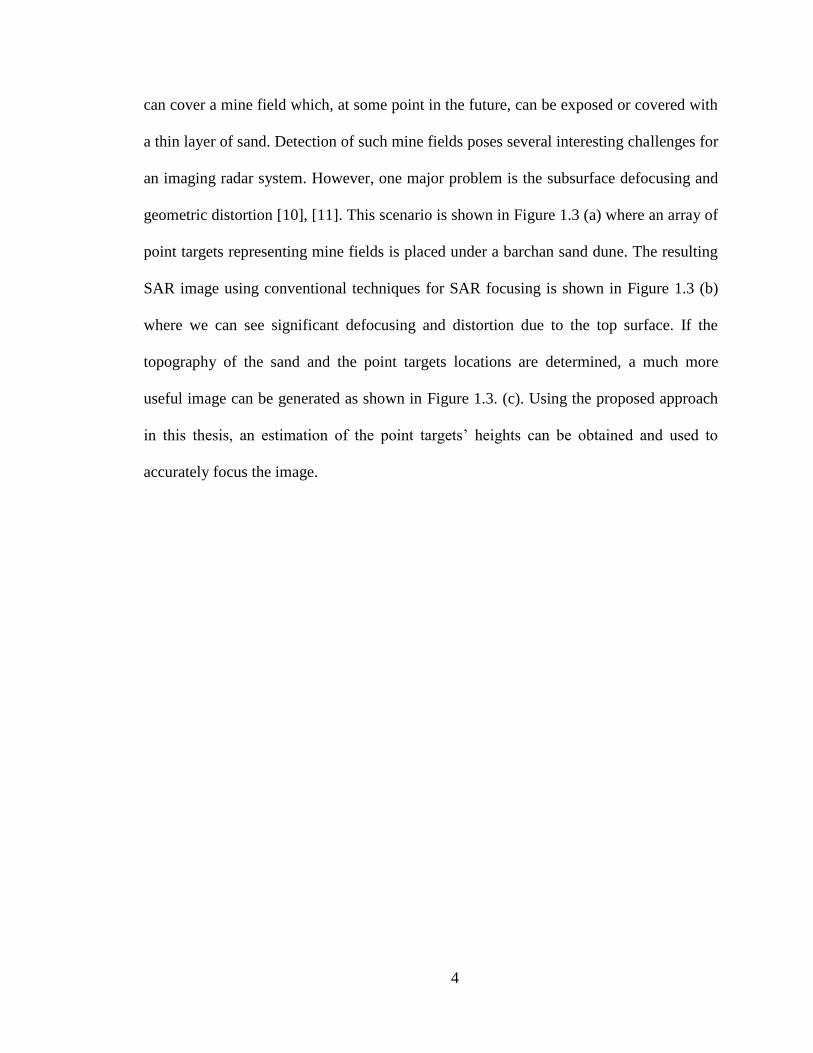
can cover a mine field which, at some point in the future, can be exposed or covered with

a thin layer of sand. Detection of such mine fields poses several interesting challenges for

an imaging radar system. However, one major problem is the subsurface defocusing and

geometric distortion [10], [11]. This scenario is shown in Figure 1.3 (a) where an array of

point targets representing mine fields is placed under a barchan sand dune. The resulting

SAR image using conventional techniques for SAR focusing is shown in Figure 1.3 (b)

where we can see significant defocusing and distortion due to the top surface. If the

topography of the sand and the point targets locations are determined, a much more

useful image can be generated as shown in Figure 1.3. (c). Using the proposed approach

in this thesis, an estimation of the point targets’ heights can be obtained and used to

accurately focus the image.

5

SAR Flight Path

Array of Ideal

Point Targets

(Not to Scale)

(a)

(b) (c)

Figure 1.3: (a) An array of point targets under a sand dune, (b) SAR image using

conventional SAR focusing and using subsurface focusing.

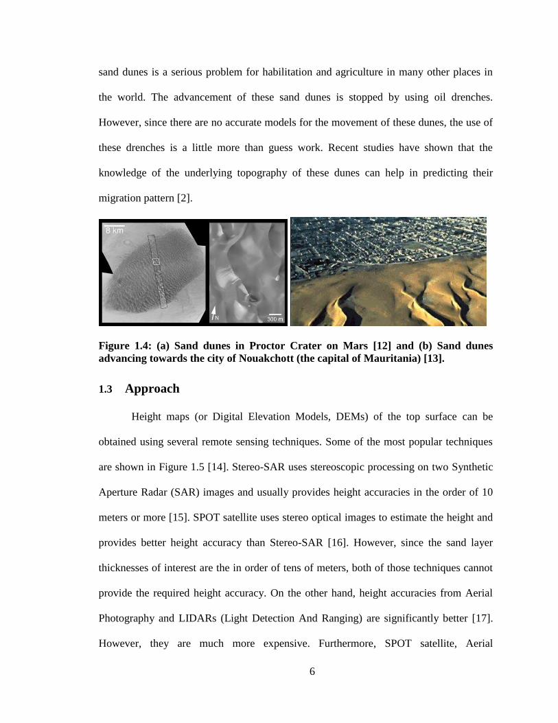
1.2.3 Other Applications

There are numerous other applications where the knowledge of the bedrock height

is very useful. For example, Figure 1.4 (a) shows sand dunes on Proctor Crater on Mars

[12]. Determination of the underlying topography in this crater can provide very useful

information such as the depth of the original crater and an estimate of the age of the

crater. Another example is shown in Figure 1.4 (b) which shows sand dunes advancing

towards the city of Nouakchott (the capital of Mauritania) [13]. The migration of these

6

sand dunes is a serious problem for habilitation and agriculture in many other places in

the world. The advancement of these sand dunes is stopped by using oil drenches.

However, since there are no accurate models for the movement of these dunes, the use of

these drenches is a little more than guess work. Recent studies have shown that the

knowledge of the underlying topography of these dunes can help in predicting their

migration pattern [2].

Figure 1.4: (a) Sand dunes in Proctor Crater on Mars [12] and (b) Sand dunes

advancing towards the city of Nouakchott (the capital of Mauritania) [13].

1.3 Approach

Height maps (or Digital Elevation Models, DEMs) of the top surface can be

obtained using several remote sensing techniques. Some of the most popular techniques

are shown in Figure 1.5 [14]. Stereo-SAR uses stereoscopic processing on two Synthetic

Aperture Radar (SAR) images and usually provides height accuracies in the order of 10

meters or more [15]. SPOT satellite uses stereo optical images to estimate the height and

provides better height accuracy than Stereo-SAR [16]. However, since the sand layer

thicknesses of interest are the in order of tens of meters, both of those techniques cannot

provide the required height accuracy. On the other hand, height accuracies from Aerial

Photography and LIDARs (Light Detection And Ranging) are significantly better [17].

However, they are much more expensive. Furthermore, SPOT satellite, Aerial

7

Photography and LIDARs are optical techniques and thus cannot be extended to also

estimate the subsurface topography. Due to these shortcomings, Airborne Interferometric

SAR (InSAR) is chosen since it provides adequate height accuracies with low cost per

Km2.

Figure 1.5: Conventional remote sensing techniques for terrain mapping [14].

An additional advantage of InSAR systems is that they can be designed and

operated over a wide range of frequencies. By choosing low operating frequency in the

VHF range, the waves can penetrate the top layer and obtain information about the

subsurface height. As will be shown in the next chapter, when using VHF InSAR data,

the top surface undulations generate artificial undulations on the estimated bottom

surface height. To remove those artifacts, information about the top surface (sand) height

is also required. Thus, another InSAR subsystem operating at Ka band is designed to map

the top surface, since at such very high frequencies the penetration depth into the top

8

layer is negligible and the Ka-InSAR provides the required top surface height information

which are then used to correct the VHF-InSAR system using a novel iterative inversion

algorithm. The proposed system is schematically shown in Figure 1.6.

Sand Surface

r

r + δr

VHF Antenna 2

Bedrock

VHF Antenna 1Ka InSAR

VHF InSARKa Antenna 1

Ka Antenna 2

Figure 1.6: The proposed dual frequency InSAR systems, Ka-InSAR provides top

surface height information that are then used to correct the VHF InSAR data to

obtain the correct subsurface height.

The required height accuracy and map resolution are in the meter range for the

proposed applications. This translates to a bandwidth of approximately 60 MHz. At Ka-

band, this corresponds to a very small fractional bandwidth (less than 1%) which makes

the antenna and the electronics design relatively straight forward. However, at VHF

frequencies, it corresponds to a relatively large fractional bandwidth (larger than 40%).

This makes the antenna design for these types of Ultra-Wideband (UWB) systems very

complex. This is mainly due to the limitations on the antenna electrical size, bandwidth

and gain [18], [19] which requires the antenna to be relatively large to achieve good gain

and very wide bandwidth. However, since these antennas are to be used for on-plane

mounting, they are required to be as compact as possible to minimize the air-drag. Thus

we investigated different designs for such antennas to minimize their overall size and

9

make them low profile. Also, as will be shown in the next chapter, InSAR systems

require a few points on the ground where the subsurface height is known. For this number

of small points, we proposed the use of Ground Penetrating Radars (GPR) which also

require compact antennas to operate at the same frequencies. And thus, we developed

several antennas for such systems as well. Such antennas are very important since they

are employed in many other systems as well such as: (1) See Through Wall Radars

where the low frequency is required to penetrate lossy walls and the large bandwidth is

required to achieve good spatial resolution [7], [20], (2) UWB communication systems

where the large bandwidth is required to achieve very high data rate and the compact size

is important to minimize the overall system size and weight [8] and (3) in UWB

localization systems where the compact size is important to minimize the size of the

localization tag and the bandwidth is required to achieve high localization accuracy [21],

[22].

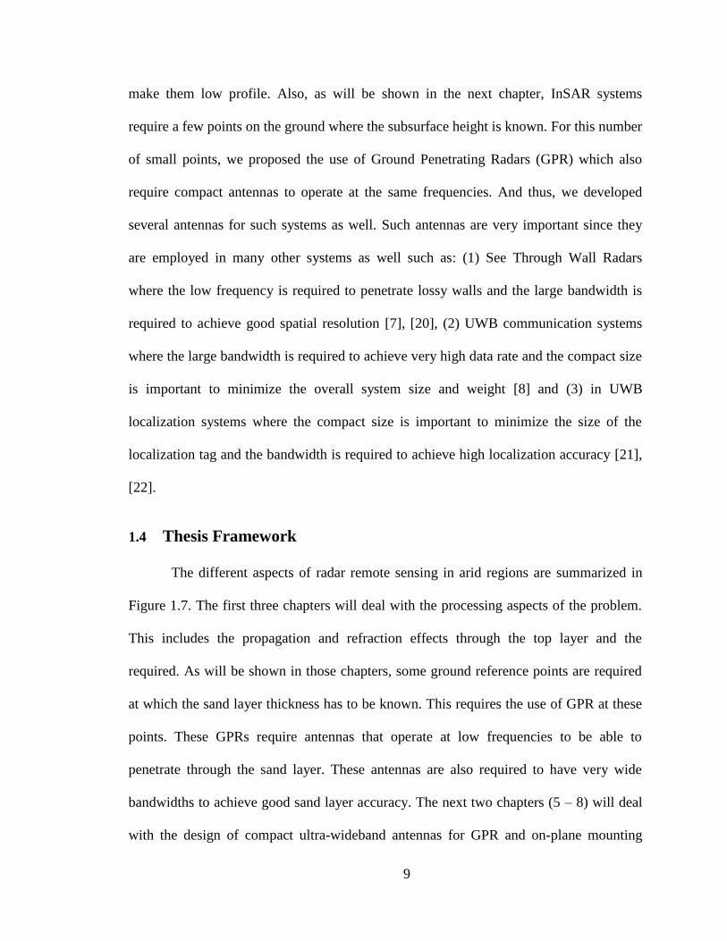
1.4 Thesis Framework

The different aspects of radar remote sensing in arid regions are summarized in

Figure 1.7. The first three chapters will deal with the processing aspects of the problem.

This includes the propagation and refraction effects through the top layer and the

required. As will be shown in those chapters, some ground reference points are required

at which the sand layer thickness has to be known. This requires the use of GPR at these

points. These GPRs require antennas that operate at low frequencies to be able to

penetrate through the sand layer. These antennas are also required to have very wide

bandwidths to achieve good sand layer accuracy. The next two chapters (5 – 8) will deal

with the design of compact ultra-wideband antennas for GPR and on-plane mounting

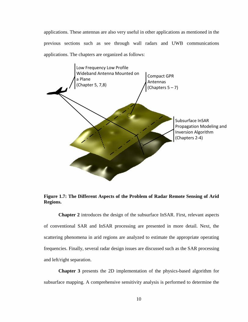
10

applications. These antennas are also very useful in other applications as mentioned in the

previous sections such as see through wall radars and UWB communications

applications. The chapters are organized as follows:

Low Frequency Low Profile Wideband Antenna Mounted on a Plane(Chapter 5, 7,8)

Compact GPR Antennas (Chapters 5 – 7)

Subsurface InSAR Propagation Modeling and Inversion Algorithm (Chapters 2-4)

Figure 1.7: The Different Aspects of the Problem of Radar Remote Sensing of Arid

Regions.

Chapter 2 introduces the design of the subsurface InSAR. First, relevant aspects

of conventional SAR and InSAR processing are presented in more detail. Next, the

scattering phenomena in arid regions are analyzed to estimate the appropriate operating

frequencies. Finally, several radar design issues are discussed such as the SAR processing

and left/right separation.

Chapter 3 presents the 2D implementation of the physics-based algorithm for

subsurface mapping. A comprehensive sensitivity analysis is performed to determine the

11

effect of the different system, noise and environment uncertainties on the accuracy of the

estimated height. The algorithm is then verified using scaled model measurements in the

lab.

A fast 3D SAR simulator based on ray tracing is presented in chapter 4. Using

the substantial speed advantage of this simulator, an efficient iterative algorithm for

subsurface SAR focusing and image coregistration is developed. The algorithm is also

verified using computer simulations and scaled model measurements in the lab.

Chapter 5 deals with the design of linearly polarized UWB antennas for radar

applications. Three antennas based on the coupled sectorial loop antenna concept are

presented. These antennas require the presence of a ground plane for operation which can

be problematic in some radar design situations. To overcome these problems, waveguide

based antennas are then developed.

Chapter 6 presents the design of UWB antennas for radar system level

implementations. In such situations, the main limiting factor is the isolation between the

transmitting and receiving antenna. This problem is discussed and the conventional

techniques are presented. Then, an antenna design is presented which provides relatively

high isolation with very small separation between the transmitting and receiving

antennas.

For radar applications, dual polarized antennas are sometimes required for clutter

reduction and/or target identification. Thus, in chapter 7 three dual polarized compact

UWB antennas based on the coupled sectorial loops antenna (CSLA) concept are

introduced. The design and principle of operation of each antenna is presented. These

12

antennas are useful for radar and communication applications. The antennas’

performance was again verified using laboratory measurements.

For on-plane mounting, two very low profile antennas are presented in chapter 8.

Those antennas are designed to have a very low profile (5% and 6% of the maximum

operating wavelength) to minimize the air drag when they are mounted on the plane

fuselage.

The conclusion and some possible future work related to the subsurface inversion

algorithm and wideband antenna design are presented in chapter 9.

13

Chapter 2

Subsurface InSAR Design

As described in the previous chapter, the optimum radar technology for mapping

the subsurface topography is Interferometric Synthetic Aperture Radar (InSAR). In this

chapter, a review on the operation of conventional InSAR systems is presented. It is

shown that conventional InSAR does not provide enough information to estimate the

subsurface topography. The required modifications of the InSAR for subsurface mapping

are then presented together with its associated design issues such as subsurface focusing

and left/right separation.

2.1 Conventional Interferometric SAR (InSAR)

The major steps for conventional InSAR processing are shown in Figure 2.1 [23].

First, two complex SAR images are generated for the same area using two slightly

different flight paths. Those two images are then coregistered to account for the scene

variations due to the different look angles. The cross-correlation of the two coregistered

images is then generated. This is done by multiplying one of the images by the complex

conjugate of the other image and then applying a moving average filter on the result. This

results in a complex amplitude cross-correlation image. The phase of the cross-

correlation image is referred to as the phase interferogram whereas the magnitude is

referred to as the coherence image and it has values in the range 0-1. The regions in the

interferogram image that have coherence values close to 1 have low phase noise whereas

regions with low coherence values have high phase noise. Phase noise affect the accuracy

14

of the height estimation using InSAR and thus several techniques are used to improve the

coherence such as interferogram filtering. The interferogram cannot be directly used to

estimate the terrain height since it is wrapped between -π and π (corresponding to the

blue and the red colors in the phase interferogram plot in Figure 2.1, respectively). Thus,

2D phase unwrapping is applied on the interferogram to obtain the absolute phase [24].

This absolute phase is then used to estimate the terrain height by knowing the height of

some reference points on the ground [25].

Generate Two SAR Images for the Same Region on the Ground

SAR Image 1

SAR Image 2

Coregister the Two Images and Generate the Phase Interferogram

Perform 2D Phase Unwrapping on the Interferogram

Phase Interfergram Unwrapped Interfergram

Using Reference Points with Known Heights on the Ground Convert the

Absolute Phase into Height

Estimated Terrain Height

Figure 2.1: Steps for generating the terrain height using InSAR.

If the above technique could be extended to mapping the subsurface; very large

regions can be mapped in a very fast and efficient way. A numerical example is shown in

Table 1, where the times required for mapping an area of 100km x 10 km are shown.

15

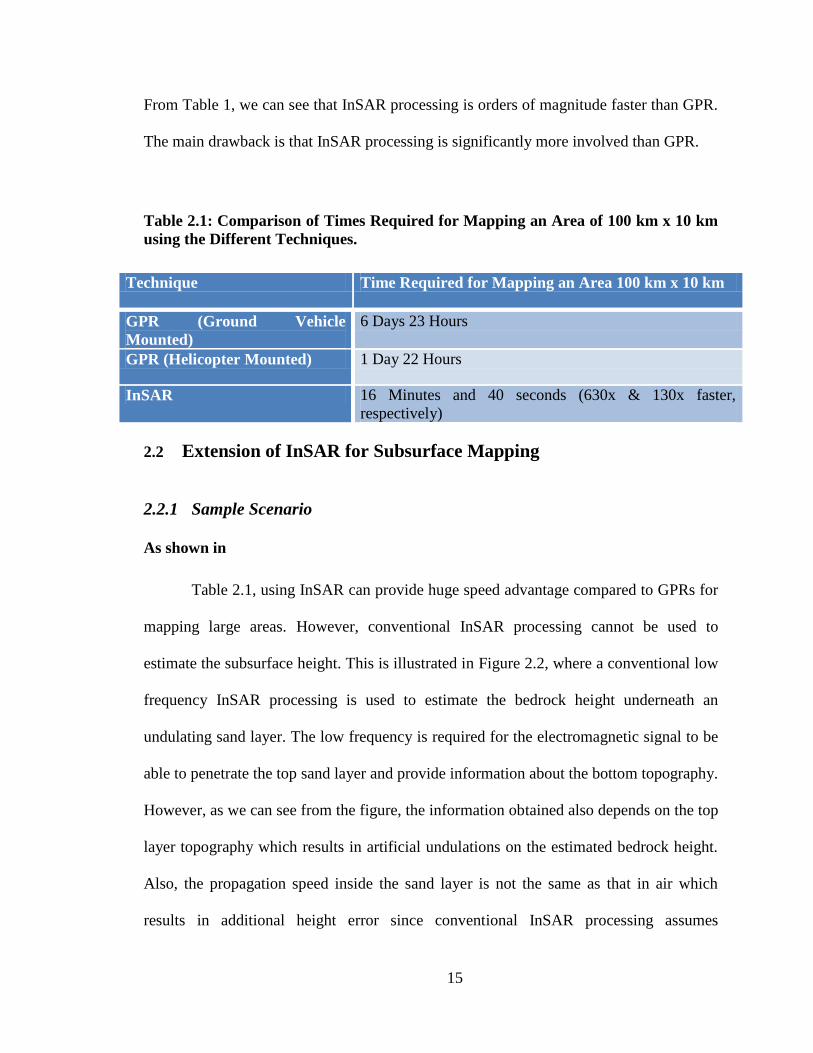
From Table 1, we can see that InSAR processing is orders of magnitude faster than GPR.

The main drawback is that InSAR processing is significantly more involved than GPR.

Table 2.1: Comparison of Times Required for Mapping an Area of 100 km x 10 km

using the Different Techniques.

Technique Time Required for Mapping an Area 100 km x 10 km

GPR (Ground Vehicle

Mounted)

6 Days 23 Hours

GPR (Helicopter Mounted) 1 Day 22 Hours

InSAR 16 Minutes and 40 seconds (630x & 130x faster,

respectively)

2.2 Extension of InSAR for Subsurface Mapping

2.2.1 Sample Scenario

As shown in

Table 2.1, using InSAR can provide huge speed advantage compared to GPRs for

mapping large areas. However, conventional InSAR processing cannot be used to

estimate the subsurface height. This is illustrated in Figure 2.2, where a conventional low

frequency InSAR processing is used to estimate the bedrock height underneath an

undulating sand layer. The low frequency is required for the electromagnetic signal to be

able to penetrate the top sand layer and provide information about the bottom topography.

However, as we can see from the figure, the information obtained also depends on the top

layer topography which results in artificial undulations on the estimated bedrock height.

Also, the propagation speed inside the sand layer is not the same as that in air which

results in additional height error since conventional InSAR processing assumes

16

propagation in air. Thus, additional information about the top layer is required as well as

modification in the InSAR processing in order to accurately estimate the subsurface

topography.

Figure 2.2: Using conventional InSAR phase-to-height equations results in severe

errors in the estimated bedrock height.

2.2.2 Proposed System

The proposed system is shown in Figure 2.2 (a) and (b) [11]. A novel two

frequency (Ka and VHF) airborne InSAR system is proposed. The Ka InSAR will be

responsible for mapping the top interface topography since at such high frequencies, the

propagation through the top layer is extremely lossy and most of the scattered waves are

coming from the top surface. The VHF InSAR will be responsible for obtaining

information about the subsurface since at these low frequencies, the waves can penetrate

the top layer with minimal attenuation and scatter from the bottom interface giving

information about its topography. The subsurface height is then obtained by correcting

for the propagation effects through the sand layer using both the Ka and VHF InSARs

data. The selection of the two frequencies is discussed in the following section.

17

Reference Plane

Sand Surface

r

r + δr

Pat

h 2

Bedrock

θs

Pat

h 1

Reference Plane

Sand Surface

r

r + δr

Pat

h 2

Bedrock

θs

Pat

h 1

Refraction at

the SurfaceDifferent

Propagation

Velocity

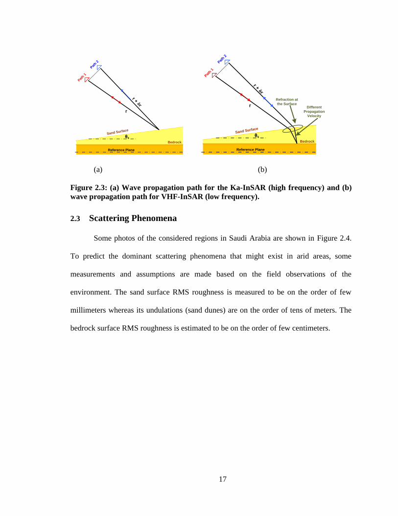
(a) (b)

Figure 2.3: (a) Wave propagation path for the Ka-InSAR (high frequency) and (b)

wave propagation path for VHF-InSAR (low frequency).

2.3 Scattering Phenomena

Some photos of the considered regions in Saudi Arabia are shown in Figure 2.4.

To predict the dominant scattering phenomena that might exist in arid areas, some

measurements and assumptions are made based on the field observations of the

environment. The sand surface RMS roughness is measured to be on the order of few

millimeters whereas its undulations (sand dunes) are on the order of tens of meters. The

bedrock surface RMS roughness is estimated to be on the order of few centimeters.

18

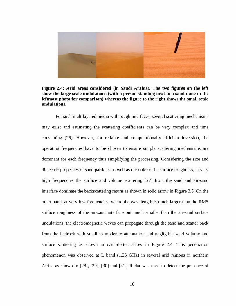
Figure 2.4: Arid areas considered (in Saudi Arabia). The two figures on the left

show the large scale undulations (with a person standing next to a sand dune in the

leftmost photo for comparison) whereas the figure to the right shows the small scale

undulations.

For such multilayered media with rough interfaces, several scattering mechanisms

may exist and estimating the scattering coefficients can be very complex and time

consuming [26]. However, for reliable and computationally efficient inversion, the

operating frequencies have to be chosen to ensure simple scattering mechanisms are

dominant for each frequency thus simplifying the processing. Considering the size and

dielectric properties of sand particles as well as the order of its surface roughness, at very

high frequencies the surface and volume scattering [27] from the sand and air-sand

interface dominate the backscattering return as shown in solid arrow in Figure 2.5. On the

other hand, at very low frequencies, where the wavelength is much larger than the RMS

surface roughness of the air-sand interface but much smaller than the air-sand surface

undulations, the electromagnetic waves can propagate through the sand and scatter back

from the bedrock with small to moderate attenuation and negligible sand volume and

surface scattering as shown in dash-dotted arrow in Figure 2.4. This penetration

phenomenon was observed at L band (1.25 GHz) in several arid regions in northern

Africa as shown in [28], [29], [30] and [31]. Radar was used to detect the presence of

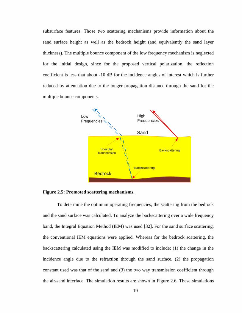
19

subsurface features. Those two scattering mechanisms provide information about the

sand surface height as well as the bedrock height (and equivalently the sand layer

thickness). The multiple bounce component of the low frequency mechanism is neglected

for the initial design, since for the proposed vertical polarization, the reflection

coefficient is less that about -10 dB for the incidence angles of interest which is further

reduced by attenuation due to the longer propagation distance through the sand for the

multiple bounce components.

Backscattering

Sand

Bedrock

Backscattering

Specular

Transmission

Low

Frequencies

High

Frequencies

Figure 2.5: Promoted scattering mechanisms.

To determine the optimum operating frequencies, the scattering from the bedrock

and the sand surface was calculated. To analyze the backscattering over a wide frequency

band, the Integral Equation Method (IEM) was used [32]. For the sand surface scattering,

the conventional IEM equations were applied. Whereas for the bedrock scattering, the

backscattering calculated using the IEM was modified to include: (1) the change in the

incidence angle due to the refraction through the sand surface, (2) the propagation

constant used was that of the sand and (3) the two way transmission coefficient through

the air-sand interface. The simulation results are shown in Figure 2.6. These simulations

20

do not include the volume scattering effects, which are relatively insignificant up to

around 10GHz [27]. The parameters used in this simulation are shown in Table 2.2. The

sand dielectric constant was measured at 150MHz and it was assumed constant with

frequency (due to insufficient measurements) as a worst case scenario, since the sand

losses increase with frequency which makes the sand backscattering even stronger at

higher frequencies. For the VHF radar, it should be noted that, from a practical

implementation point of view, the higher the operating frequency is the better the

performance for several reasons, namely: (1) higher operating frequency simplifies the

radar antenna and system design, (2) allows for higher bandwidth (and consequently

higher resolution) for the same system complexity (same relative bandwidth) and (3)

allows for using geometrical optics modeling for faster undulations in sand geometries

(since the limitation of geometrical optics is that the radius of curvature of the sand

undulations has to be much larger than the wavelength [33]). VHF SARs have been used

in several applications such as target detection under foliage and terrain mapping [6], [34]

and [35].

21

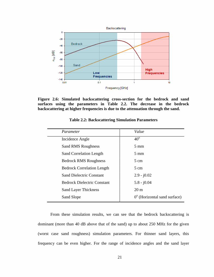
Figure 2.6: Simulated backscattering cross-section for the bedrock and sand

surfaces using the parameters in Table 2.2. The decrease in the bedrock

backscattering at higher frequencies is due to the attenuation through the sand.

Table 2.2: Backscattering Simulation Parameters

Parameter Value

Incidence Angle 40o

Sand RMS Roughness 5 mm

Sand Correlation Length 5 mm

Bedrock RMS Roughness 5 cm

Bedrock Correlation Length 5 cm

Sand Dielectric Constant 2.9 - j0.02

Bedrock Dielectric Constant 5.8 - j0.04

Sand Layer Thickness 20 m

Sand Slope 0o (Horizontal sand surface)

From these simulation results, we can see that the bedrock backscattering is

dominant (more than 40 dB above that of the sand) up to about 250 MHz for the given

(worst case sand roughness) simulation parameters. For thinner sand layers, this

frequency can be even higher. For the range of incidence angles and the sand layer

22

thicknesses considered, an operating frequency of about 150 MHz was chosen for the low

frequency radar. On the other hand, for the high frequencies, since sand surface has very

low RMS roughness in some areas, the volume scattering component must be considered

as the dominant source of backscattering. Using random media theory, it was determined

that to get sufficient volume backscattering from a smooth flat sand surface, the operating

frequency has to be in Ka band (at about 35 GHz) as shown in Figure 2.7.

Figure 2.7: Numerically calculated backscattering coefficient of the c50-70 sand

layer as a function of radar frequency. The sand layer was assumed 0.15 m thick,

has 0.6 in volume fraction (from [36]).

2.4 Subsurface InSAR Processing

As shown in Figure 2.3, the conventional InSAR processing is adequate for Ka-

band InSAR data. That is, two SAR images are generated from two slightly different

flight passes (antennas 1 and 2). The two images are then co-registered and the phase

interferogram and the coherence maps are generated. Finally, the phase interferogram is

unwrapped and the terrain height is estimated using ground control points (GCP).

23

However, for VHF InSAR, several issues appear due to refraction and propagation of the

signal in the sand layer. In this section, we will briefly highlight some of the processing

issues and artifacts that appear due to these effects.

2.4.1 Subsurface Focusing

The first step in the InSAR processing is the generation of the SAR images.

However, conventional SAR focusing does not correct for the refraction and propagation

effects inside the sand as previously discussed. In order to quantify the resulting error

when using conventional SAR processing for subsurface focusing, the scenario shown in

Figure 2.8 was simulated, where an ideal point target was placed under flat horizontal

sand at a depth of Zt. The radar height and point target ground range are 5km and 2km

respectively. The simulated center frequency is 150MHz and the bandwidth is 60MHz.

The raw data was then generated using a subsurface SAR simulator that includes the

frequency dependent attenuation and dispersion through the sand as well as the refraction

and the different propagation velocity. The focusing was performed using the

conventional back-projection technique [37] with a focusing plane at the sand surface

using different integration angles. The integration angle is calculated as

. The point target responses along the range and azimuth were normalized and

displaced to a reference point to compare the image distortion.

24

Sand Surface

Flight Path

Ground Range

Azimuth

5 K

m

Zt

Point Target

θi

θf

Figure 2.8: Simulation Scenario for VHF SAR focusing on a point target at depth Zt

below the sand surface.

The result is shown in Figure 2.9 (a)-(d). The range point spread function (PSF)

section is almost independent on the integration angle and shows minimal distortion as

expected due to the relatively low loss and dispersion of the sand at such low frequencies.

However, there is significant distortion in the azimuth direction for large integration

angles. This distortion is due to the fact that the standard focusing technique does not

account for the sand propagation and refraction. However, as we can see from Figure 2.9

(b)-(d), by decreasing the integration angle, the SAR depth of focus is increased and thus

a well-focused image can be obtained at the expense of reduced resolution. However,

since the developed algorithm (Chapter 3) can estimate the target (bedrock) height, this

information can be fed back into the SAR focusing and a higher resolution image can

then be obtained through an iterative process. This will be shown in Chapter 4.

2.4.2 Image Coregistration

Due to the refraction through an undulating sand surface, the image will be

distorted even if the bedrock is flat. An example is shown in Figure 2.10 where 56

25

uniformly distributed point targets are placed at a constant depth under an undulating

sand surface. The raw SAR data was generated and focused using a conventional back

projection processor with adjusted integration angle to achieve good focusing as

discussed in the previous subsection. From Figure 2.10, we can see that the targets’

image has been distorted due to the top surface topography. This could lead to significant

coregistration error for relatively large baselines. For the baseline values considered in

this thesis, the coregistration error was found to be relatively small when using

conventional coregistration methods and the unequal ground range displacements are

corrected through the proposed algorithm as will be shown in Chapter 3. However, for

larger baselines (which might be required to achieve higher height accuracy), adaptive

co-registration techniques have to be used.

26

Range Section (20o Integration Angle)

Displaced Ground Range [m]

-30 -20 -10 0 10 20 30

Norm

aliz

ed A

mplit

ude

-0.2

0.0

0.2

0.4

0.6

0.8

1.0

1.2

Zt = 0 m

Zt = -10 m

Zt = -20 m

Zt = -30 m

Azimuth Section (20o Integration Angle)

Cross Range [m]

-30 -20 -10 0 10 20 30

Norm

aliz

ed A

mplit

ude

-0.2

0.0

0.2

0.4

0.6

0.8

1.0

1.2

Zt = 0 m

Zt = -10 m

Zt = -20 m

Zt = -30 m

(a) (b)


Cross Range [m]

-30 -20 -10 0 10 20 30

Norm

aliz

ed A

mplit

ude

-0.2

0.0

0.2

0.4

0.6

0.8

1.0

1.2

Zt = 0 m

Zt = -10 m

Zt = -20 m

Zt = -30 m


Cross Range [m]

-30 -20 -10 0 10 20 30

No

rma

lize

d A

mp

litu

de

-0.2

0.0

0.2

0.4

0.6

0.8

1.0

1.2

Zt = 0 m

Zt = -10 m

Zt = -20 m

Zt = -30 m

(c) (d)

Figure 2.9: (a) PSF range section, (b) PSF azimuth section for 20o integration angle,

(c) PSF azimuth section for 15o integration angle and (d) PSF azimuth section for

10o integration angle.

Array of Ideal

Point Targets

(Not to Scale)

Sand Surface

(a) (b)

Figure 2.10: Image distortion due to top surface undulations (a) geometry and (b)

focused SAR image.

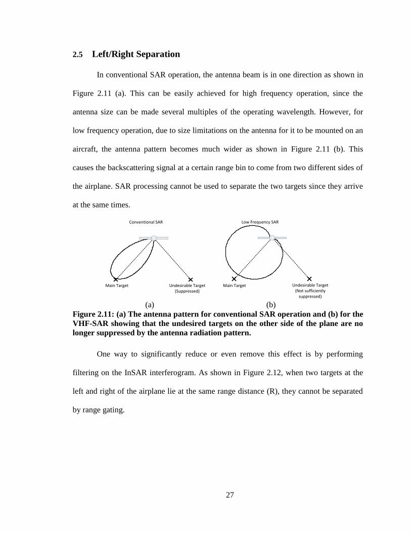
27

2.5 Left/Right Separation

In conventional SAR operation, the antenna beam is in one direction as shown in

Figure 2.11 (a). This can be easily achieved for high frequency operation, since the

antenna size can be made several multiples of the operating wavelength. However, for

low frequency operation, due to size limitations on the antenna for it to be mounted on an

aircraft, the antenna pattern becomes much wider as shown in Figure 2.11 (b). This

causes the backscattering signal at a certain range bin to come from two different sides of

the airplane. SAR processing cannot be used to separate the two targets since they arrive

at the same times.

Undesirable Target(Not sufficiently

suppressed)

Undesirable Target(Suppressed)

Main Target

Conventional SAR Low Frequency SAR

Main Target

(a) (b)

Figure 2.11: (a) The antenna pattern for conventional SAR operation and (b) for the

VHF-SAR showing that the undesired targets on the other side of the plane are no

longer suppressed by the antenna radiation pattern.

One way to significantly reduce or even remove this effect is by performing

filtering on the InSAR interferogram. As shown in Figure 2.12, when two targets at the

left and right of the airplane lie at the same range distance (R), they cannot be separated

by range gating.

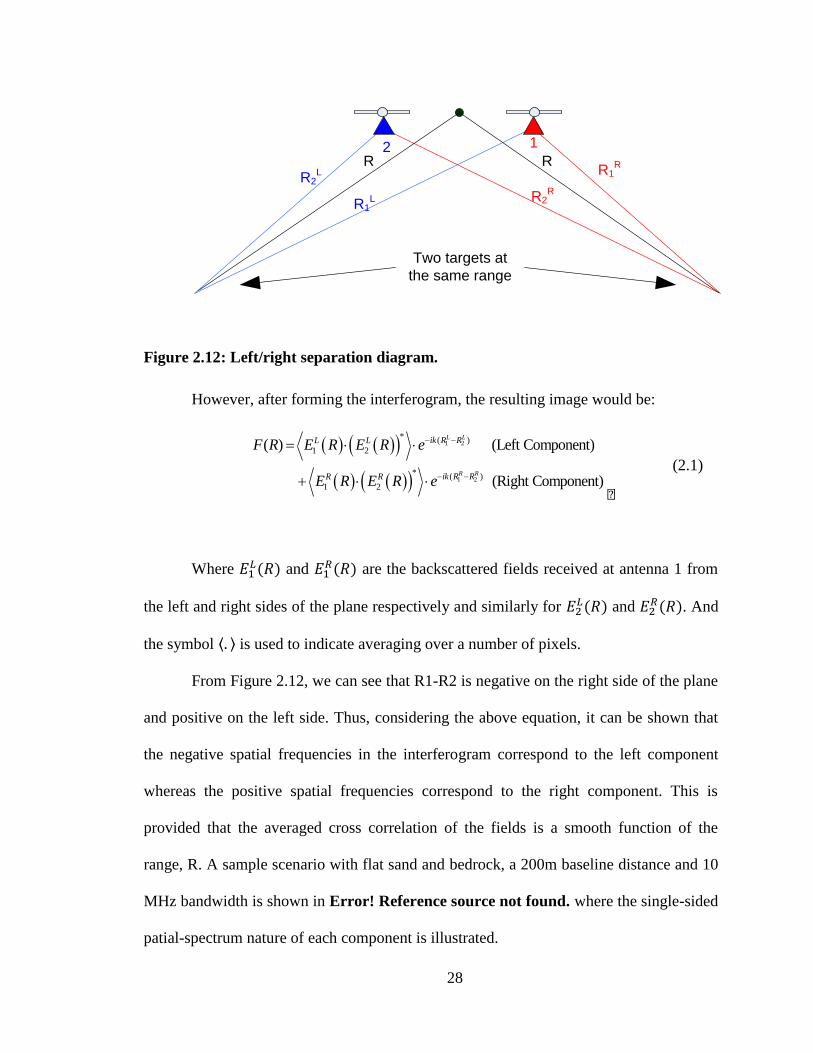
28

Two targets at

the same range

R1R

R2R

R1L

R2L

12R R

Figure 2.12: Left/right separation diagram.

However, after forming the interferogram, the resulting image would be:

1 2

1 2

* ( )

1 2

* ( )

1 2

( ) (Left Component)

(Right Component)

L L

R R

ik R RL L

ik R RR R

F R E R E R e

E R E R e

(2.1)

Where and

are the backscattered fields received at antenna 1 from

the left and right sides of the plane respectively and similarly for and

. And

the symbol ⟨ ⟩ is used to indicate averaging over a number of pixels.

From Figure 2.12, we can see that R1-R2 is negative on the right side of the plane

and positive on the left side. Thus, considering the above equation, it can be shown that

the negative spatial frequencies in the interferogram correspond to the left component

whereas the positive spatial frequencies correspond to the right component. This is

provided that the averaged cross correlation of the fields is a smooth function of the

range, R. A sample scenario with flat sand and bedrock, a 200m baseline distance and 10

MHz bandwidth is shown in Error! Reference source not found. where the single-sided

patial-spectrum nature of each component is illustrated.

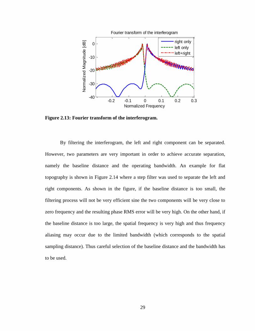
29

Figure 2.13: Fourier transform of the interferogram.

By filtering the interferogram, the left and right component can be separated.

However, two parameters are very important in order to achieve accurate separation,

namely the baseline distance and the operating bandwidth. An example for flat

topography is shown in Figure 2.14 where a step filter was used to separate the left and

right components. As shown in the figure, if the baseline distance is too small, the

filtering process will not be very efficient sine the two components will be very close to

zero frequency and the resulting phase RMS error will be very high. On the other hand, if

the baseline distance is too large, the spatial frequency is very high and thus frequency

aliasing may occur due to the limited bandwidth (which corresponds to the spatial

sampling distance). Thus careful selection of the baseline distance and the bandwidth has

to be used.

-0.2 -0.1 0 0.1 0.2 0.3-40

-30

-20

-10

0

Normalized Frequency

Norm

alized M

agnitude [

dB

]

Fourier transform of the interferogram

right only

left only

left+right

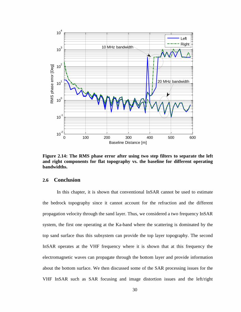
30

Figure 2.14: The RMS phase error after using two step filters to separate the left

and right components for flat topography vs. the baseline for different operating

bandwidths.

2.6 Conclusion

In this chapter, it is shown that conventional InSAR cannot be used to estimate

the bedrock topography since it cannot account for the refraction and the different

propagation velocity through the sand layer. Thus, we considered a two frequency InSAR

system, the first one operating at the Ka-band where the scattering is dominated by the

top sand surface thus this subsystem can provide the top layer topography. The second

InSAR operates at the VHF frequency where it is shown that at this frequency the

electromagnetic waves can propagate through the bottom layer and provide information

about the bottom surface. We then discussed some of the SAR processing issues for the

VHF InSAR such as SAR focusing and image distortion issues and the left/right

0 100 200 300 400 500 60010

-2

10-1

100

101

102

103

104

Baseline Distance [m]

RM

S p

hase e

rror

[Deg]

Left

Right10 MHz bandwidth

20 MHz bandwidth

31

separation due to the low directivity of plane mounted antennas at VHF frequencies. In

the following chapter, an inversion algorithm is presented that combines the data from the

VHF and the Ka InSAR to correct for the refraction and the propagation through the top

layer and provide an estimation of the bedrock height.

32

Chapter 3

Subsurface Topography Inversion Algorithm

The issues associated with the subsurface mapping InSAR design were addressed

in the previous chapter. As was shown, conventional InSAR processing cannot be used to

map the subsurface topography and modification in the processing has to be performed.

In this chapter, the inversion technique that uses both the Ka- and VHF-InSAR data to

obtain the subsurface height is discussed and its sensitivity to the different system and

environment parameters is analyzed. The accuracy of the algorithm was verified using

numerical simulations as well as scaled model measurements.

3.1 Subsurface Propagation Modeling

For the subsurface VHF InSAR processing, the conventional InSAR phase-to-

height equations has to be modified to correct for the refraction and the different

propagation speed inside the sand. For sand geometries with radii of curvature that are

much larger than the wavelength (which is the aim of this paper), geometrical optics can

be used to accurately relate the phase difference to the height. The geometry is shown in

Figure 3.1 and the system of nonlinear equations relating the phase difference to the

bedrock height and sand height and slope is summarized in Table 3.1. All the symbols

refer to the VHF InSAR parameters except for hs(y) which refers to the sand height map

obtained using the Ka-InSAR with conventional InSAR processing where hs is the sand

height and y is the ground range. All the dimensions and angles are in general dependent

on the ground range (y) and/or radar azimuth position (x). In these equations, 2D sand

33

geometry is assumed (no variation with x). However, the extension for arbitrary 3D

variations is straightforward by adjusting the azimuth position of the bedrock

backscattering point according to the refraction through the sand surface.

Table 3.1: The system of nonlinear equations describing the phase difference

between the two SAR images (m=1,2).

Description Equation

Snell’s Law

Geometry

Ground Range

Electrical Range

Phase Difference

Sand Map

α

B

H

hs2

hb

θi1

θi2

θt1

θt2

ψ1

ψ2

Sand Surface

Bedrock Surface

Arbitrary Reference Plane

θs

Y

Z

X

Antenna 2

(x,yr2,hr2)

Antenna 1

(x,yr1,hr1)

ys1

ys2

yb

hs

1

Figure 3.1: Geometrical optics modeling for subsurface imaging VHF InSAR (not to

scale for clarity).

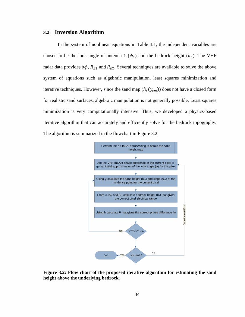
34

3.2 Inversion Algorithm

In the system of nonlinear equations in Table 3.1, the independent variables are

chosen to be the look angle of antenna 1 ( ) and the bedrock height ( ). The VHF

radar data provides , and . Several techniques are available to solve the above

system of equations such as algebraic manipulation, least squares minimization and

iterative techniques. However, since the sand map ( ) does not have a closed form

for realistic sand surfaces, algebraic manipulation is not generally possible. Least squares

minimization is very computationally intensive. Thus, we developed a physics-based

iterative algorithm that can accurately and efficiently solve for the bedrock topography.

The algorithm is summarized in the flowchart in Figure 3.2.

Perform the Ka InSAR processing to obtain the sand

height map

Use the VHF InSAR phase difference at the current pixel to

get an initial approximation of the look angle (ψ) for this pixel

Using ψ calculate the sand height (hs1) and slope (θs1) at the

incidence point for the current pixel

From ψ, hs1 and θs1 calculate bedrock height (hb) that gives

the correct pixel electrical range

Using h calculate θ that gives the correct phase difference δφ

|h(n+1)

- h(n)

| < Δ

Last pixel ?End

No

Go

to

th

e n

ext P

ixe

l

YesNo

Figure 3.2: Flow chart of the proposed iterative algorithm for estimating the sand

height above the underlying bedrock.

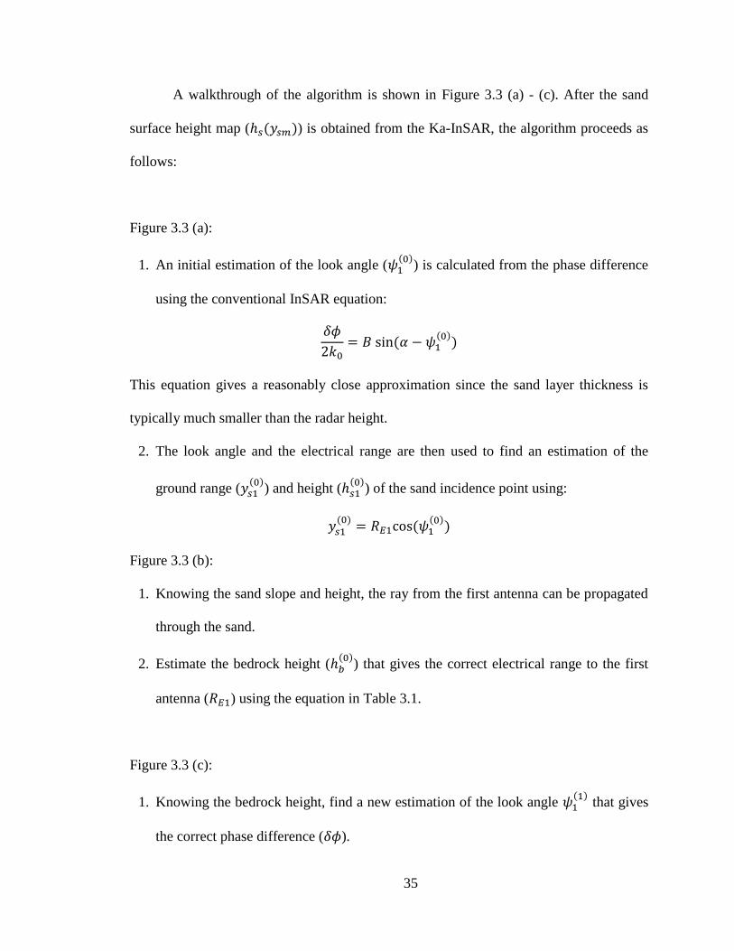
35

A walkthrough of the algorithm is shown in Figure 3.3 (a) - (c). After the sand

surface height map ( ) is obtained from the Ka-InSAR, the algorithm proceeds as

follows:

Figure 3.3 (a):

1. An initial estimation of the look angle (

) is calculated from the phase difference

using the conventional InSAR equation:

This equation gives a reasonably close approximation since the sand layer thickness is

typically much smaller than the radar height.

2. The look angle and the electrical range are then used to find an estimation of the

ground range (

) and height (

) of the sand incidence point using:

Figure 3.3 (b):

1. Knowing the sand slope and height, the ray from the first antenna can be propagated

through the sand.

2. Estimate the bedrock height (

) that gives the correct electrical range to the first

antenna ( ) using the equation in Table 3.1.

Figure 3.3 (c):

1. Knowing the bedrock height, find a new estimation of the look angle

that gives

the correct phase difference ( ).

36

2. Knowing the new look angle and the bedrock height, find a new estimation of the

sand incidence point height and slope.

The process (b)-(c) is repeated until the magnitude of the change in the estimated

bedrock height between two successive iterations is less than a prescribed

error tolerance, . Also, at this stage, the correct ground range of the scattering point

( ) is already calculated.

The proposed algorithm was tested for several ideal and realistic sand surfaces

and bedrock scenarios and was found to converge in less than 5 iterations in most cases.

Some examples are shown in Figure 3.4 (a) and (b). The raw InSAR data for these

examples were generated using geometrical optics modeling.

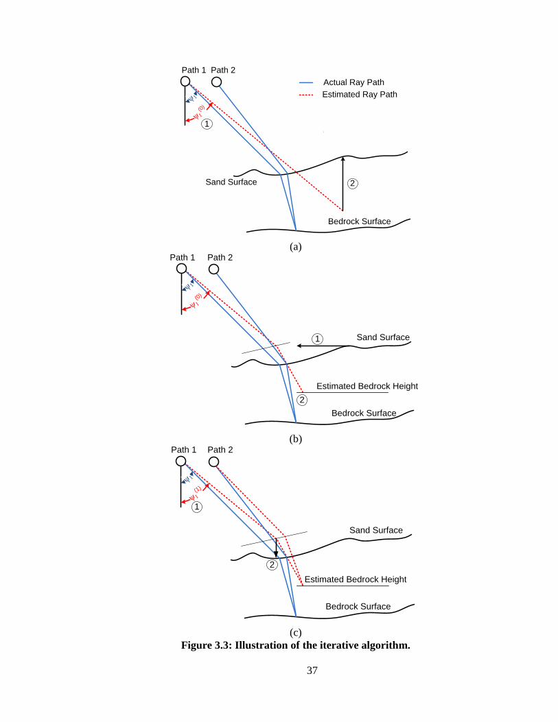
37

Sand Surface

Bedrock Surface

Path 1 Path 2

Actual Ray Path

Estimated Ray Pathψ 1

ψ 1(0

)

1

2

(a)

Sand Surface

Bedrock Surface

Path 1 Path 2

ψ 1

ψ 1(0

)

Estimated Bedrock Height

1

2

(b)

Sand Surface

Bedrock Surface

Path 1 Path 2

ψ 1

ψ 1(1

)

Estimated Bedrock Height

1

2

(c)

Figure 3.3: Illustration of the iterative algorithm.

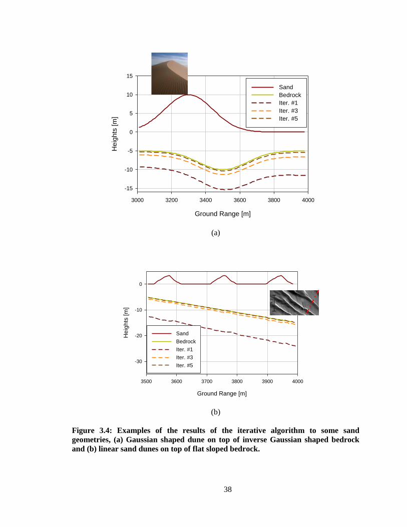
38

Ground Range [m]

3000 3200 3400 3600 3800 4000

He

igh

ts [

m]

-15

-10

-5

0

5

10

15

Sand

Bedrock

Iter. #1

Iter. #3

Iter. #5

(a)

Ground Range [m]

3500 3600 3700 3800 3900 4000

He

igh

ts [

m]

-30

-20

-10

0

Sand

Bedrock

Iter. #1

Iter. #3

Iter. #5

(b)

Figure 3.4: Examples of the results of the iterative algorithm to some sand

geometries, (a) Gaussian shaped dune on top of inverse Gaussian shaped bedrock

and (b) linear sand dunes on top of flat sloped bedrock.

39

3.3 Sensitivity Analysis of the Height Estimation

Due to the unavoidable system errors and physical limitations, a sensitivity

analysis has to be performed to characterize the height estimation accuracy in the

presence of such errors. In this section, we summarize the limits of the height estimation

accuracy due to errors in the sand dielectric constant as well as system limitations. The

sand/bedrock scenario used in this section consists of flat horizontal bedrock underneath

a flat sand with slope . In the following, unless otherwise stated, the dimensions are as

summarized in Table 3.2 (the dimensions are defined in Figure 3.1).

Table 3.2: Sensitivity Analysis Scenario Parameters

Parameter Value Parameter Value

(Baseline Angle) 90o yb (Bedrock Ground Range) 3.5km

B (Baseline Distance) 100m hb(yb) (Bedrock Height) 0m

H (Platform Height) 5km hs(yb) (Sand Height) 10m

(Sand layer slope) 0o Sand Layer Thickness (hs(yb) - hb(yb)) 10 m

Figure 3.5 shows the sensitivity of the inversion algorithm to errors in the sand

dielectric constant. We can see that the percentage height error is relatively small for

small variations in the sand dielectric constant for most realistic sand slopes. Similar

results were obtained for different sand and bedrock scenarios. This allows the use of the

proposed technique for different regions or slightly inhomogeneous sand layers with

relatively small errors.

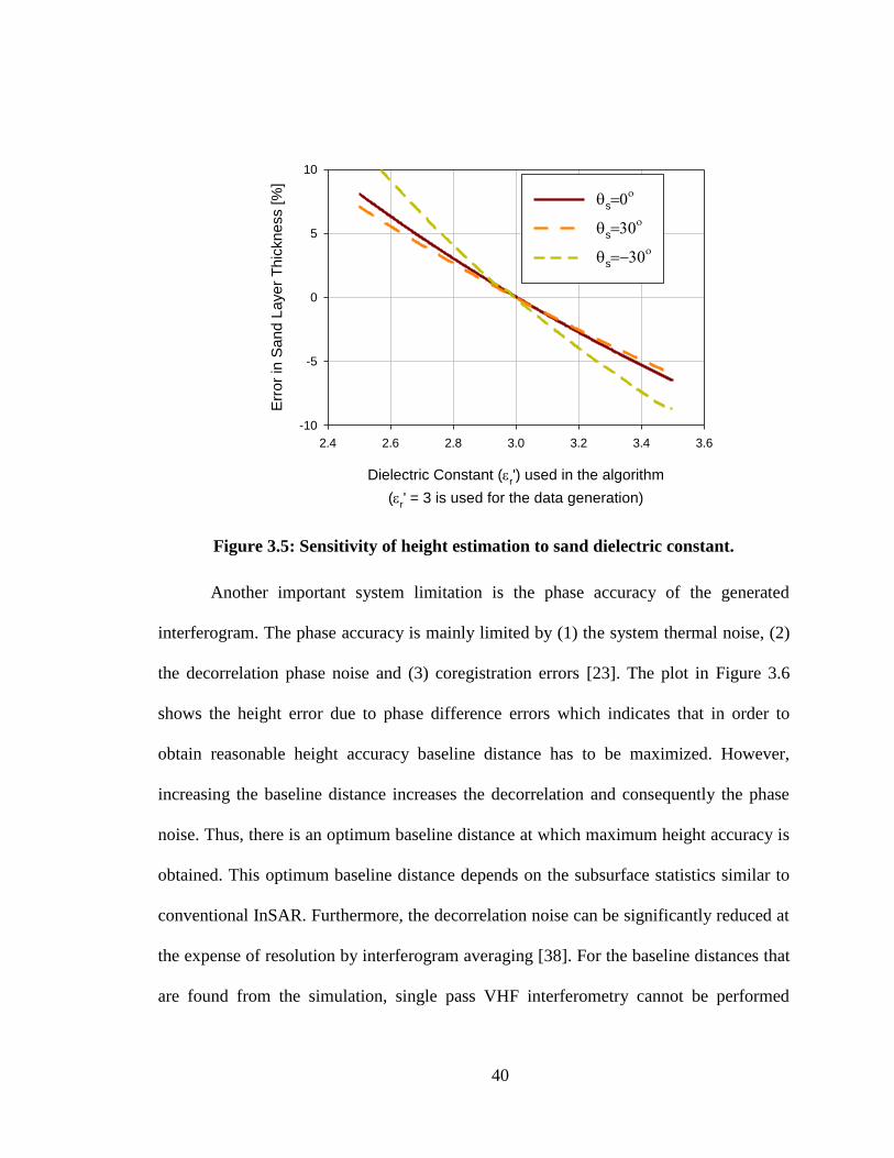
40

Dielectric Constant (r') used in the algorithm

(r' = 3 is used for the data generation)

2.4 2.6 2.8 3.0 3.2 3.4 3.6

Err

or

in S

an

d L

aye

r T

hic

kn

ess [

%]

-10

-5

0

5

10

s

s

s

Figure 3.5: Sensitivity of height estimation to sand dielectric constant.

Another important system limitation is the phase accuracy of the generated

interferogram. The phase accuracy is mainly limited by (1) the system thermal noise, (2)

the decorrelation phase noise and (3) coregistration errors [23]. The plot in Figure 3.6

shows the height error due to phase difference errors which indicates that in order to

obtain reasonable height accuracy baseline distance has to be maximized. However,

increasing the baseline distance increases the decorrelation and consequently the phase

noise. Thus, there is an optimum baseline distance at which maximum height accuracy is

obtained. This optimum baseline distance depends on the subsurface statistics similar to

conventional InSAR. Furthermore, the decorrelation noise can be significantly reduced at

the expense of resolution by interferogram averaging [38]. For the baseline distances that

are found from the simulation, single pass VHF interferometry cannot be performed

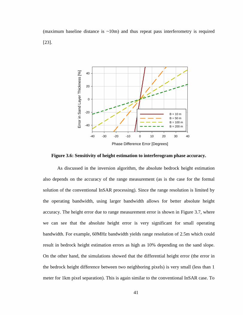
41

(maximum baseline distance is ~10m) and thus repeat pass interferometry is required

[23].

Phase Difference Error [Degrees]

-40 -30 -20 -10 0 10 20 30 40

Err

or

in S

an

d L

aye

r T

hic

kn

ess [

%]

-40

-20

0

20

40

B = 10 m

B = 50 m

B = 100 m

B = 200 m

Figure 3.6: Sensitivity of height estimation to interferogram phase accuracy.

As discussed in the inversion algorithm, the absolute bedrock height estimation

also depends on the accuracy of the range measurement (as is the case for the formal

solution of the conventional InSAR processing). Since the range resolution is limited by

the operating bandwidth, using larger bandwidth allows for better absolute height

accuracy. The height error due to range measurement error is shown in Figure 3.7, where

we can see that the absolute height error is very significant for small operating

bandwidth. For example, 60MHz bandwidth yields range resolution of 2.5m which could

result in bedrock height estimation errors as high as 10% depending on the sand slope.

On the other hand, the simulations showed that the differential height error (the error in

the bedrock height difference between two neighboring pixels) is very small (less than 1

meter for 1km pixel separation). This is again similar to the conventional InSAR case. To

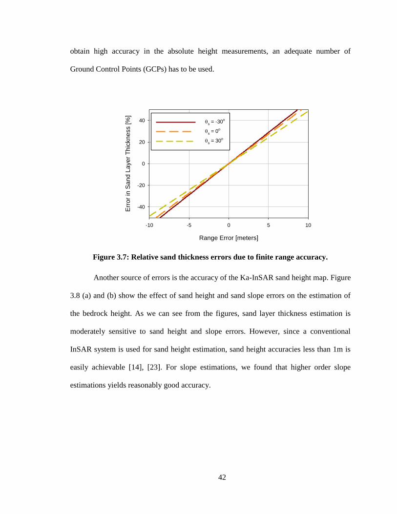
42

obtain high accuracy in the absolute height measurements, an adequate number of

Ground Control Points (GCPs) has to be used.

Range Error [meters]

-10 -5 0 5 10

Err

or

in S

an

d L

aye

r T

hic

kn

ess [

%]

-40

-20

0

20

40 s = -30

o

s = 0

o

s = 30

o

Figure 3.7: Relative sand thickness errors due to finite range accuracy.

Another source of errors is the accuracy of the Ka-InSAR sand height map. Figure

3.8 (a) and (b) show the effect of sand height and sand slope errors on the estimation of

the bedrock height. As we can see from the figures, sand layer thickness estimation is

moderately sensitive to sand height and slope errors. However, since a conventional

InSAR system is used for sand height estimation, sand height accuracies less than 1m is

easily achievable [14], [23]. For slope estimations, we found that higher order slope

estimations yields reasonably good accuracy.

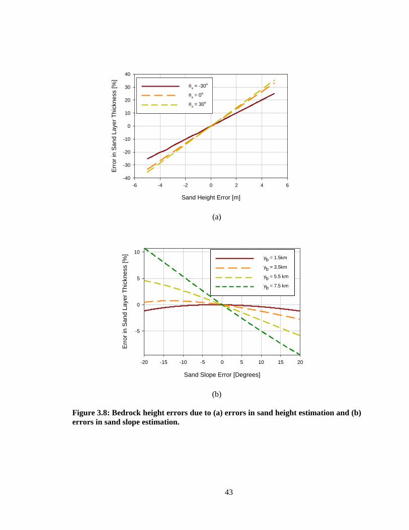
43

Sand Height Error [m]

-6 -4 -2 0 2 4 6

Err

or

in S

an

d L

aye

r T

hic

kn

ess [

%]

-40

-30

-20

-10

0

10

20

30

40

s = -30

o

s = 0

o

s = 30

o

(a)

Sand Slope Error [Degrees]

-20 -15 -10 -5 0 5 10 15 20

Err

or

in S

an

d L

aye

r T

hic

kn

ess [

%]

-5

0

5

10yb = 1.5km

yb = 3.5km

yb = 5.5 km

yb = 7.5 km

(b)

Figure 3.8: Bedrock height errors due to (a) errors in sand height estimation and (b)

errors in sand slope estimation.

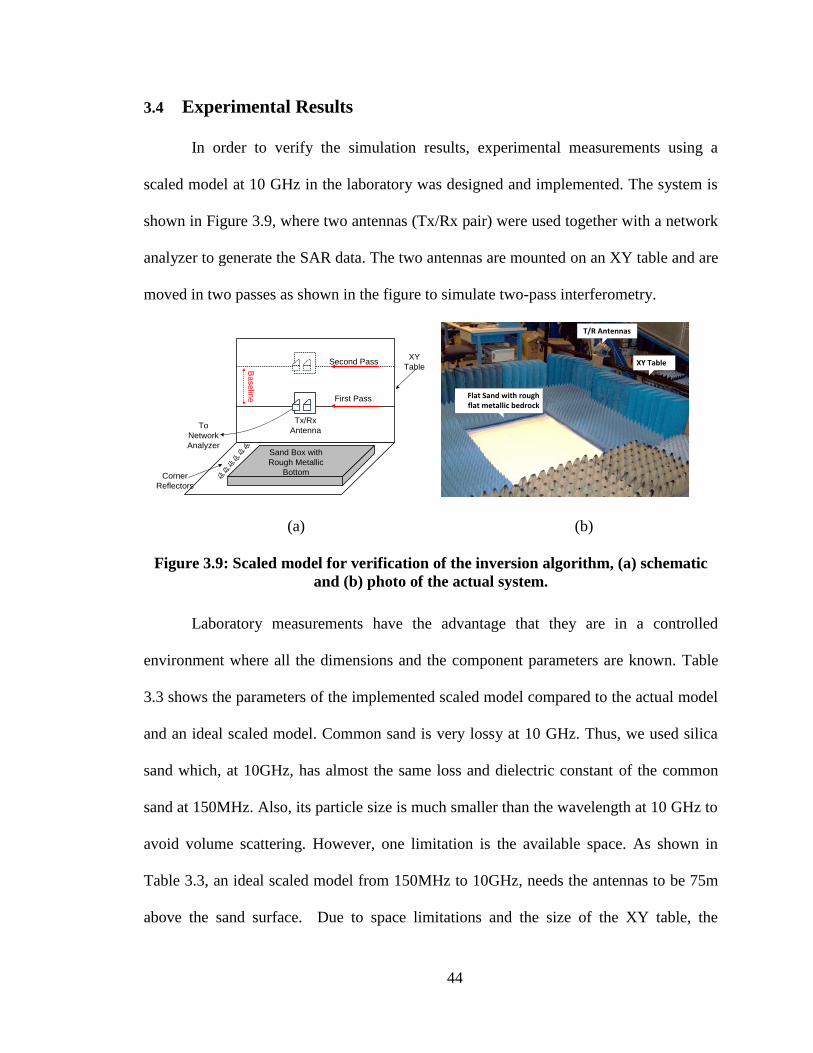
44

3.4 Experimental Results

In order to verify the simulation results, experimental measurements using a

scaled model at 10 GHz in the laboratory was designed and implemented. The system is

shown in Figure 3.9, where two antennas (Tx/Rx pair) were used together with a network

analyzer to generate the SAR data. The two antennas are mounted on an XY table and are

moved in two passes as shown in the figure to simulate two-pass interferometry.

To

Network

Analyzer

Tx/Rx

Antenna

Ba

se

line First Pass

Second Pass

Sand Box with

Rough Metallic

Bottom

XY

Table

Corner

Reflectors

T/R Antennas

Flat Sand with rough flat metallic bedrock

XY Table

(a) (b)

Figure 3.9: Scaled model for verification of the inversion algorithm, (a) schematic

and (b) photo of the actual system.

Laboratory measurements have the advantage that they are in a controlled

environment where all the dimensions and the component parameters are known. Table

3.3 shows the parameters of the implemented scaled model compared to the actual model

and an ideal scaled model. Common sand is very lossy at 10 GHz. Thus, we used silica

sand which, at 10GHz, has almost the same loss and dielectric constant of the common

sand at 150MHz. Also, its particle size is much smaller than the wavelength at 10 GHz to

avoid volume scattering. However, one limitation is the available space. As shown in

Table 3.3, an ideal scaled model from 150MHz to 10GHz, needs the antennas to be 75m

above the sand surface. Due to space limitations and the size of the XY table, the

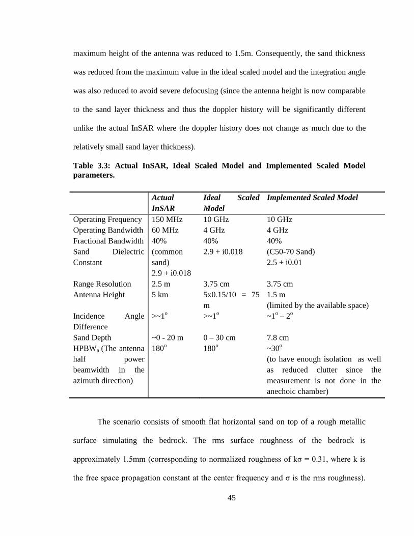
45

maximum height of the antenna was reduced to 1.5m. Consequently, the sand thickness

was reduced from the maximum value in the ideal scaled model and the integration angle

was also reduced to avoid severe defocusing (since the antenna height is now comparable

to the sand layer thickness and thus the doppler history will be significantly different

unlike the actual InSAR where the doppler history does not change as much due to the

relatively small sand layer thickness).

Table 3.3: Actual InSAR, Ideal Scaled Model and Implemented Scaled Model

parameters.

Actual

InSAR

Ideal Scaled

Model

Implemented Scaled Model

Operating Frequency 150 MHz 10 GHz 10 GHz

Operating Bandwidth 60 MHz 4 GHz 4 GHz

Fractional Bandwidth 40% 40% 40%

Sand Dielectric

Constant

(common

sand)

2.9 + i0.018

2.9 + i0.018 (C50-70 Sand)

2.5 + i0.01

Range Resolution 2.5 m 3.75 cm 3.75 cm

Antenna Height 5 km 5x0.15/10 = 75

m

1.5 m

(limited by the available space)

Incidence Angle

Difference

>~1o

>~1o

~1o – 2

o

Sand Depth ~0 - 20 m 0 – 30 cm

7.8 cm

HPBWa (The antenna

half power

beamwidth in the

azimuth direction)

180o 180

o ~30

o

(to have enough isolation as well

as reduced clutter since the

measurement is not done in the

anechoic chamber)

The scenario consists of smooth flat horizontal sand on top of a rough metallic

surface simulating the bedrock. The rms surface roughness of the bedrock is

approximately 1.5mm (corresponding to normalized roughness of kζ = 0.31, where k is

the free space propagation constant at the center frequency and ζ is the rms roughness).

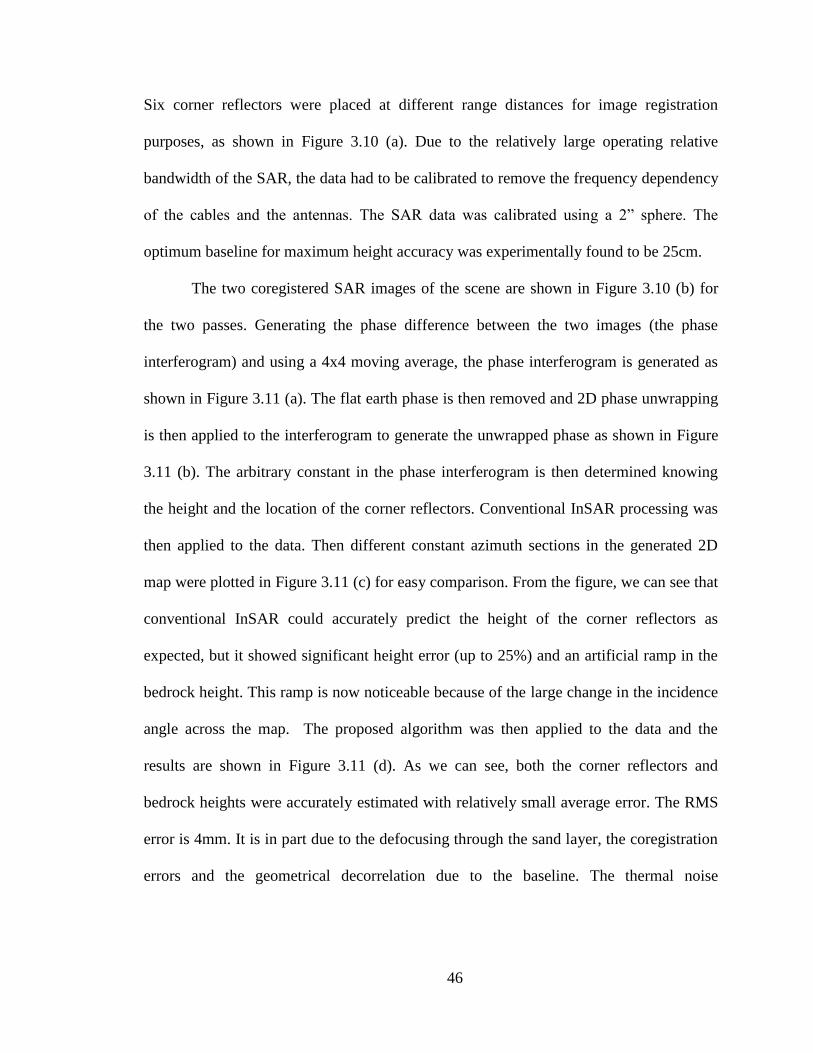
46

Six corner reflectors were placed at different range distances for image registration

purposes, as shown in Figure 3.10 (a). Due to the relatively large operating relative

bandwidth of the SAR, the data had to be calibrated to remove the frequency dependency

of the cables and the antennas. The SAR data was calibrated using a 2‖ sphere. The

optimum baseline for maximum height accuracy was experimentally found to be 25cm.

The two coregistered SAR images of the scene are shown in Figure 3.10 (b) for

the two passes. Generating the phase difference between the two images (the phase

interferogram) and using a 4x4 moving average, the phase interferogram is generated as

shown in Figure 3.11 (a). The flat earth phase is then removed and 2D phase unwrapping

is then applied to the interferogram to generate the unwrapped phase as shown in Figure

3.11 (b). The arbitrary constant in the phase interferogram is then determined knowing

the height and the location of the corner reflectors. Conventional InSAR processing was

then applied to the data. Then different constant azimuth sections in the generated 2D

map were plotted in Figure 3.11 (c) for easy comparison. From the figure, we can see that

conventional InSAR could accurately predict the height of the corner reflectors as

expected, but it showed significant height error (up to 25%) and an artificial ramp in the

bedrock height. This ramp is now noticeable because of the large change in the incidence

angle across the map. The proposed algorithm was then applied to the data and the

results are shown in Figure 3.11 (d). As we can see, both the corner reflectors and

bedrock heights were accurately estimated with relatively small average error. The RMS

error is 4mm. It is in part due to the defocusing through the sand layer, the coregistration

errors and the geometrical decorrelation due to the baseline. The thermal noise

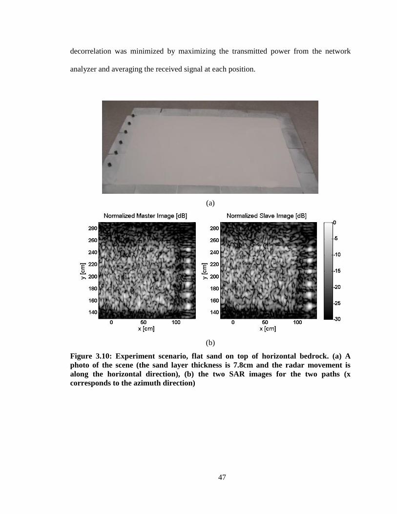
47

decorrelation was minimized by maximizing the transmitted power from the network

analyzer and averaging the received signal at each position.

(a)

(b)

Figure 3.10: Experiment scenario, flat sand on top of horizontal bedrock. (a) A

photo of the scene (the sand layer thickness is 7.8cm and the radar movement is

along the horizontal direction), (b) the two SAR images for the two paths (x

corresponds to the azimuth direction)

48

(a) (b)

(c) (d)

Figure 3.11: Scaled Model Results: (a) The averaged interforogram (4x4 boxcar

averaging), (b) the unwrapped interferogram, (c) the estimated heights using the

conventional InSAR and (d) the estimated heights using the proposed algorithm.

3.5 Conclusion

In this chapter, an inversion algorithm was presented that is able to use the sand

map from the Ka-InSAR and the generated interferogram from the VHF-InSAR to

estimate the bottom surface topography. The algorithm employs geometrical optics to

model the propagation of the electromagnetic waves through the top surface. Some

49

scenarios for different top and bottom surfaces were simulated and it was shown that the

proposed algorithm converges to the correct height within a few iterations. The effect of

several the system and environment parameters on the height estimation accuracy was

analyzed. It is shown that the baseline distance has to be at least a few tens of meters to

achieve good height accuracy and thus single pass interferometry (two antennas mounted

on the same plane) cannot be used. It is also shown that the height estimation is not very

sensitive to the sand dielectric constant and thus slight sand inhomogeneities do not affect

the bedrock height estimation. The algorithm was then verified using scaled model

measurements in the lab.

50

Chapter 4

Image Distortion Effects in SAR Subsurface Imaging and a

New Iterative Approach for Refocusing and Coregistration

In chapter 2, the effects of the defocusing and geometric aberrations in the

subsurface SAR images were briefly discussed. Unfortunately, these aberrations cannot

be corrected without the knowledge of the bottom surface topography which in turn is

obtained from the subsurface SAR images using the algorithm described in chapter 3.

Thus, in this chapter we propose an iterative approach where the SAR images are formed

using conventional processing. Next, the subsurface inversion algorithm is used to obtain

the subsurface height which is then used to refocus the images and remove the geometric

aberration. The process is then repeated iteratively. We first present a fast subsurface

SAR simulator that can generate the SAR data for arbitrary sand geometries. This

simulator is then used to investigate the different image aberrations that result from the

top surface topography including geometric and defocusing distortion. Next, the issue of

subsurface caustics and their effect on the imaging is discussed. Then the iterative

approach to estimate and correct for such aberrations is presented. It is shown using

simulations and measurements that up to an order of magnitude improvement in the

subsurface image resolution as well as significant improvement on subsurface

interferogam coherence can be achieved. The approach is verified theoretically using 3D

simulations and experimentally using scaled model measurements in the lab.

51

4.1 Fast Subsurface SAR Simulator & Subsurface Focusing Technique

The raw baseband range-compressed SAR image is a function of the radar

position, xj (slow time) and pulse time, t (fast time). For a number of discrete targets

located at (xi, yi, zi), it can be expressed as [39]:

( )

∑

( ) ( ( ( )

)) (

( )

)

( )

(4.1)

where, C1 is a constant that is dependent on the radar system parameters and the

antenna gain, N is the number of scattering points in the scene, Ai(xj)=A(xj, xi, yi, zi) is

an amplitude and phase factor that is dependent on the antenna radiation pattern and the

transmission coefficient through the sand, B is the operating bandwidth, c is the speed of

light in free space, ω0 is the center angular frequency and Ri(xj) = R(xj, xi, yi, zi) is the

effective range to each target defined as:

( ) | |

, (4.2)

where , , are the position vectors of the radar, the incidence point and

the target, respectively as shown in Figure 4.1.

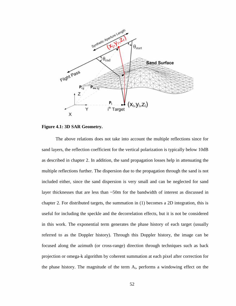
52

Pr,j Pinc I,j

Pi

Figure 4.1: 3D SAR Geometry.

The above relations does not take into account the multiple reflections since for

sand layers, the reflection coefficient for the vertical polarization is typically below 10dB

as described in chapter 2. In addition, the sand propagation losses help in attenuating the

multiple reflections further. The dispersion due to the propagation through the sand is not

included either, since the sand dispersion is very small and can be neglected for sand

layer thicknesses that are less than ~50m for the bandwidth of interest as discussed in

chapter 2. For distributed targets, the summation in (1) becomes a 2D integration, this is

useful for including the speckle and the decorrelation effects, but it is not be considered

in this work. The exponential term generates the phase history of each target (usually

referred to as the Doppler history). Through this Doppler history, the image can be

focused along the azimuth (or cross-range) direction through techniques such as back

projection or omega-k algorithm by coherent summation at each pixel after correction for

the phase history. The magnitude of the term Ai, performs a windowing effect on the

53

phase history and thus limits the resolution, whereas its phase variation causes distortion

to the phase history and should be minimized through careful antenna and system design

and/or calibration.

The ray path for a point target under an arbitrary sand geometry is shown in

Figure 4.1. The direct method to form the raw SAR data (generate Ri(xj) and Ai(xj)), is by

solving the system of nonlinear equations describing the ray propagation through the sand

surface for each target and each radar position. Here it is assumed that air-sand interface

profile is known. It should be noted that in real practice the air-sand interface profile can

be obtained directly using a high-frequency (Ka-band) InSAR. The direct method for

generating raw SAR data for large number of targets is extremely time consuming. Thus,

we developed a much faster and relatively accurate technique which can efficiently

generate the raw SAR data for large number of targets without the computational cost of

solving a large set of nonlinear equations. The approach can be summarized as follows

(see Figure 4.2):

1. The sand surface is triangulated using a suitable resolution. Next, at each radar

position, xj, a number of rays are launched from the radar to the center of each

sand surface facet.

2. Those rays are then refracted through the sand facets using geometrical optics and

propagated through the sand in ΔR steps as shown in Figure 4.2. The electrical

range to the radar, Rn(xj, xn, yn, zn) and losses An(xj, xn, yn, zn), are recorded at

each ΔR step.

3. This results in the knowledge of the effective range and losses over the non-

uniform grid (xn, yn, zn). Using interpolation over a non-uniform grid we can

54

obtain the electrical range and losses to each target (xi, yi, zi). We found that the

required number of grid points (xn, yn, zn) to achieve good range accuracy is

relatively small since the range function is a relatively smooth function of the

position for practical sand surfaces and radar heights as shown in the contour in

Figure 4.2.

4. This process is then repeated at each radar position xj to obtain the full phase

history for each point in the scene. This technique is much faster since

interpolation is a much less computationally intensive operation compared to the

solution of nonlinear equations. However, interpolation can only be performed

when there are no caustic conditions (ray intersection). For the considered sand

layer depths and sand angle of repose (maximum slope), caustic conditions

happen relatively rarely. In the regions where they occur, simple ray tracing

cannot be used and a more rigorous approach has to be employed such as

MLFMM or Physical Optics.

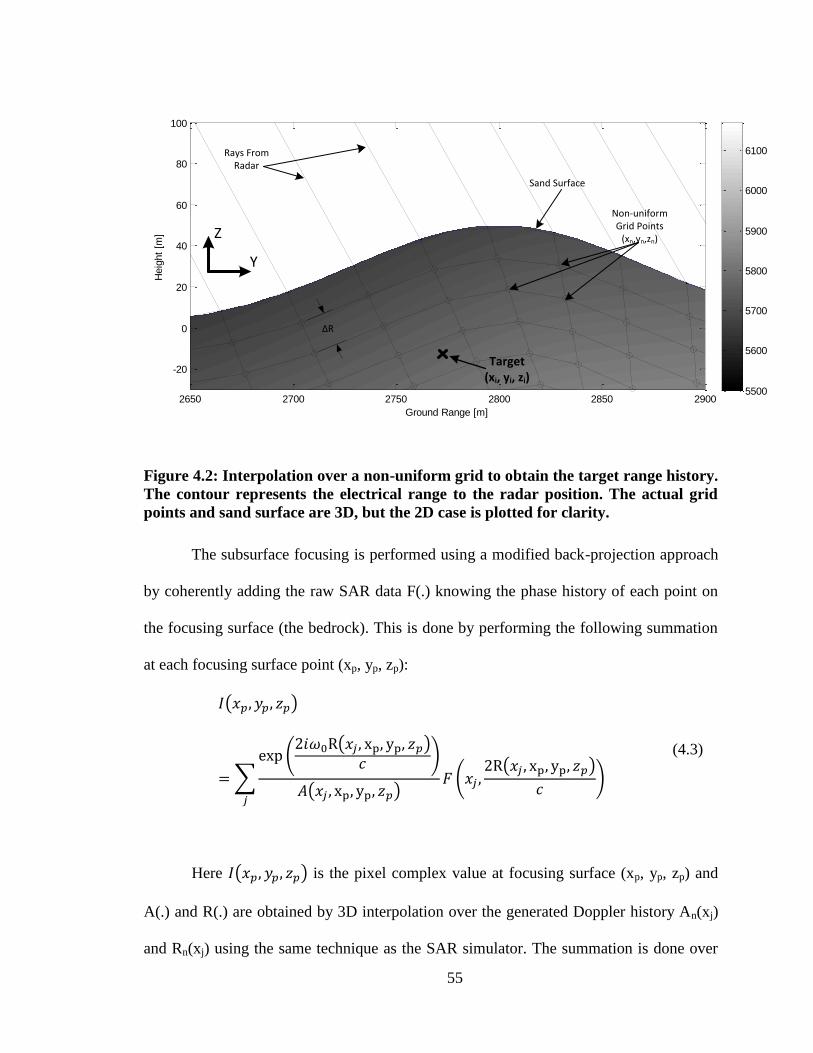
55

Ground Range [m]

Heig

ht

[m]

2650 2700 2750 2800 2850 2900

-20

0

20

40

60

80

100

5500

5600

5700

5800

5900

6000

6100Rays From Radar

Sand Surface

Non-uniform Grid Points

(xn,yn,zn)

Target (xi, yi, zi)

ΔR

Y

Z

Figure 4.2: Interpolation over a non-uniform grid to obtain the target range history.

The contour represents the electrical range to the radar position. The actual grid

points and sand surface are 3D, but the 2D case is plotted for clarity.

The subsurface focusing is performed using a modified back-projection approach

by coherently adding the raw SAR data F(.) knowing the phase history of each point on

the focusing surface (the bedrock). This is done by performing the following summation

at each focusing surface point (xp, yp, zp):

( )

∑

( ( )

)

( )

( ( )

)

(4.3)

Here ( ) is the pixel complex value at focusing surface (xp, yp, zp) and

A(.) and R(.) are obtained by 3D interpolation over the generated Doppler history An(xj)

and Rn(xj) using the same technique as the SAR simulator. The summation is done over

56

the desired synthetic aperture length (or equivalently the integration angle, θend - θstart) as

shown in Figure 4.1. The amplitude term is omitted in the focusing since it tends to

amplify the noise and it is very hard to accurately estimate the sand losses. Thus, the

subsurface focused image can be formally written as:

( )

∑ ( ( )

)

( ( )

)

(4.4)

4.2 Defocusing and Distortion Effects in SAR Subsurface Imaging

Conventional SAR processing assumes that the ray path between the radar and the

target is a straight line with a propagation constant equal to that of free space. For

subsurface targets with top surface undulations, this results in two types of SAR image

artifacts: 1) defocusing and 2) geometrical distortion. Furthermore, other geometric

distortion effects common to conventional SAR, such as foreshortening and layover, also

appear, but these become a function of the geometry of the top surface in addition to the

bottom surface. In this section, we present these effects on some practical scenarios. The

simulations in this section assumes a radar center frequency of 150 MHz, the bandwidth

is 60MHz and the platform height is 5 Km.

4.2.1 Defocusing Effects

The first problem with subsurface SAR images are defocusing effects which can

be separated into range defocusing and azimuth defocusing. Simulation results shows that

range defocusing is much less significant than azimuth defocusing since dry sand

dispersion is very small for the frequency range considered in this application as shown

57

in Chapter 2. However, azimuth defocusing is very significant and poses significant

limitation on the achievable azimuth resolution. An example is shown in Figure 4.3

where a target was placed under a sand layer with flat interface at a ground range of 2km

and a depth of Zt that is varied from 0 - 40m. The target image was generated using

conventional back-projection with focusing plane at the top surface. Figure 4.3 (a) shows

that for small integration angle, the azimuth point spread function (APSF) of the target

maintains its form up to a depth of approximately 20m (corresponding to long depth of

focus) but has poor ground resolution. On the other hand, for larger integration angles

(Figure 4.3 (b)), the APSF has much better ground resolution but keeps its form over

much shorter distance of about 5m, beyond which the resolution degrades rapidly (short

depth of focus). This is compared to the same target in air in Figure 4.3 (c) and (d), where

we can see that the depth of focus is much larger and thus conventional SAR images does

not require refocusing for small height perturbations unlike subsurface images. It should

also be noted that for VHF SARs due to the low operating frequency and the limitations

on the antenna sizes, larger integration angles are typically required to both achieve

reasonable ground resolution as well as good SNR (e.g. 120o is used in [5]). Thus,

accurate focusing is extremely important from both an image resolution and clutter

reduction point of views.

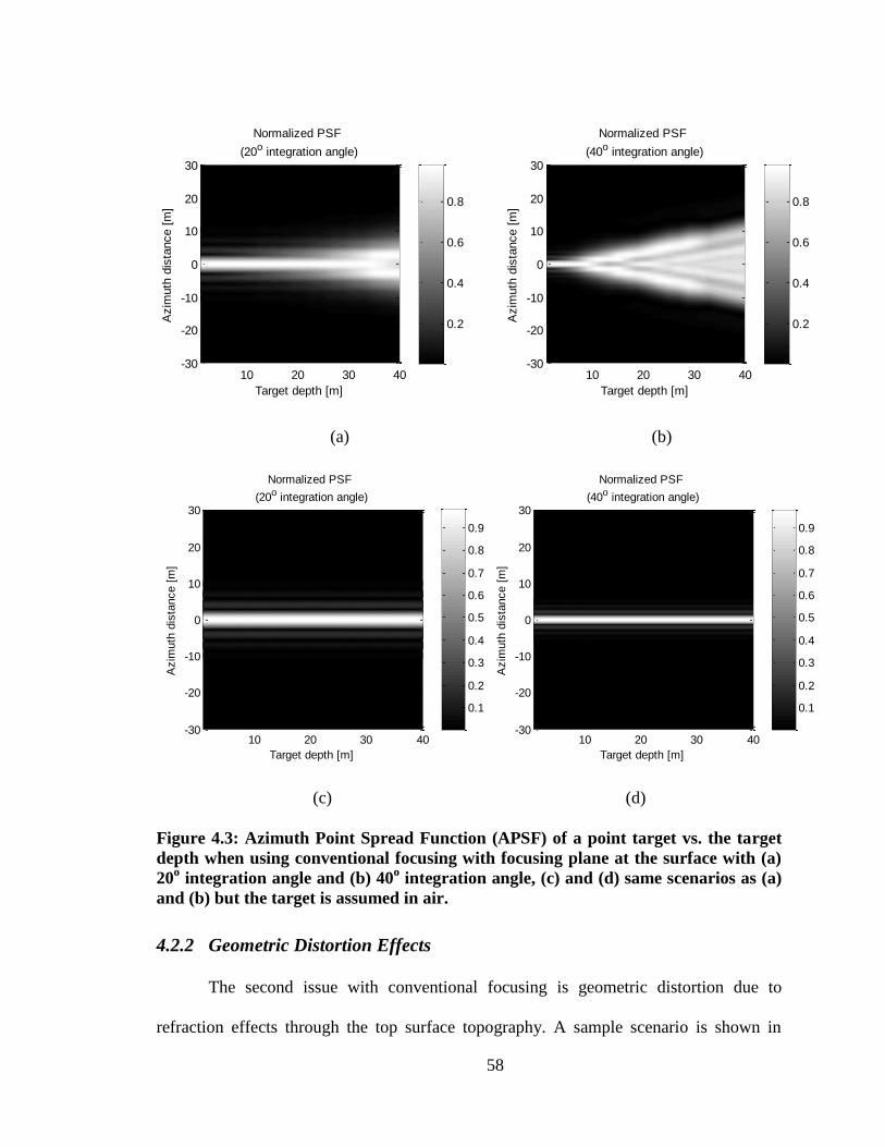
58

(a) (b)

(c) (d)

Figure 4.3: Azimuth Point Spread Function (APSF) of a point target vs. the target

depth when using conventional focusing with focusing plane at the surface with (a)

20o integration angle and (b) 40

o integration angle, (c) and (d) same scenarios as (a)

and (b) but the target is assumed in air.

4.2.2 Geometric Distortion Effects

The second issue with conventional focusing is geometric distortion due to

refraction effects through the top surface topography. A sample scenario is shown in

Normalized PSF

(20o integration angle)

Target depth [m]

Azim

uth

dis

tance [

m]

10 20 30 40-30

-20

-10

0

10

20

30

0.2

0.4

0.6

0.8

Normalized PSF


Target depth [m]

Azim

uth

dis

tance [

m]

10 20 30 40-30

-20

-10

0

10

20

30

0.2

0.4

0.6

0.8

Normalized PSF


Target depth [m]

Azim

uth

dis

tance [

m]

10 20 30 40-30

-20

-10

0

10

20

30

Normalized PSF


Target depth [m]

Azim

uth

dis

tance [

m]

10 20 30 40-30

-20

-10

0

10

20

30

0.1

0.2

0.3

0.4

0.5

0.6

0.7

0.8

0.9

0.1

0.2

0.3

0.4

0.5

0.6

0.7

0.8

0.9

59

Figure 4.4 (a), where an array of 121 (11x11) point targets arranged uniformly over an

azimuth range of 200m and ground range of 200m centered at (0, 2Km) is placed at a

depth of 5 m under a Gaussian shaped sand dune with crest height of 15m and length of

100m. The integration angle was limited to 10o to avoid defocusing as discussed in the

previous section. We can see that the point target locations are shifted due to the

refraction through the top layer. The two shown effects in Figure 4.4 (b) correspond to

foreshortening and elongation using conventional SAR processing. This limits the use of

the subsurface InSAR in some applications such as mine detection. It also affects the

image coregistration accuracy resulting in lower InSAR coherence since these distortion

effects are strong function of the look angle. For larger slopes and/or deeper targets,

foreshortening can become a special form of layover where caustic target location

ambiguity can occur.

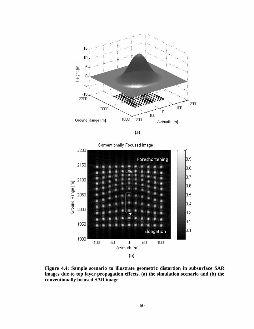
60

(b)

Foreshortening

Elongation

(a)

Figure 4.4: Sample scenario to illustrate geometric distortion in subsurface SAR

images due to top layer propagation effects, (a) the simulation scenario and (b) the

conventionally focused SAR image.

61

4.2.3 Caustic Surfaces and their Effects

Caustic (or focal) surfaces exist at ray intersections due to phase front aberrations

at which the conventional geometrical optics solution is invalid and either extensions to

physical optics (PO) or other numerical technique have to be used to estimate the fields at

these locations. As mentioned before, the top air-sand interface curvature is large for

mast sand dune surfaces encountered. For these conditions, caustic surfaces generally

exist at depths beyond the sand layer thickness above the bedrock. However, it is

interesting to show how the caustic surfaces can be estimated and some of the geometric

distortions that are introduced due caustics. It should be noted that the caustic surfaces

change according to the source location (radar position) and thus have to be estimated at

each position along the radar path.

4.2.3.1 Estimation of caustic surfaces

Estimation of caustic surfaces is a common problem in computer graphics [40],

[41]. One common approach to characterize the caustic surface is the Jacobian method

[40], [42]. This method is summarized as follows: the points along a ray emanating from

the center of the surface triangular facet i downwards can be parameterized as:

(4.5)

Here is the coordinate vector of the center of the triangular facet i, is

the sand surface height function and is the unit vector along the direction of

propagation into the sand.

The refractive caustic surface (denoted as ) is tangential to the refracted rays at

one or more points, thus for the ith

ray, the caustic surface lies at certain u termed as uc:

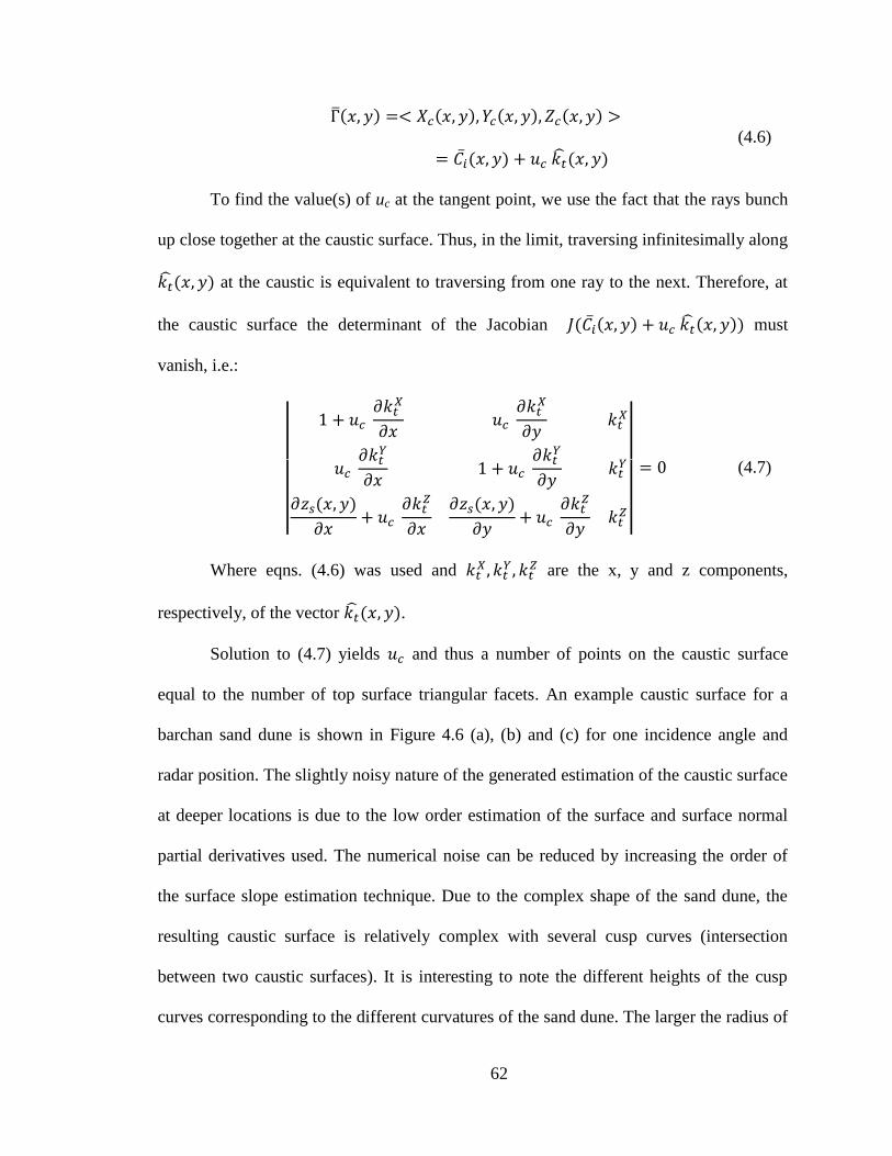
62

(4.6)

To find the value(s) of uc at the tangent point, we use the fact that the rays bunch

up close together at the caustic surface. Thus, in the limit, traversing infinitesimally along

at the caustic is equivalent to traversing from one ray to the next. Therefore, at

the caustic surface the determinant of the Jacobian must

vanish, i.e.:

|

|

|

|

(4.7)

Where eqns. (4.6) was used and

are the x, y and z components,

respectively, of the vector .

Solution to (4.7) yields and thus a number of points on the caustic surface

equal to the number of top surface triangular facets. An example caustic surface for a

barchan sand dune is shown in Figure 4.6 (a), (b) and (c) for one incidence angle and

radar position. The slightly noisy nature of the generated estimation of the caustic surface

at deeper locations is due to the low order estimation of the surface and surface normal

partial derivatives used. The numerical noise can be reduced by increasing the order of

the surface slope estimation technique. Due to the complex shape of the sand dune, the

resulting caustic surface is relatively complex with several cusp curves (intersection

between two caustic surfaces). It is interesting to note the different heights of the cusp

curves corresponding to the different curvatures of the sand dune. The larger the radius of

63

curvature, the larger is the depth of the cusp curves as shown by the dotted arrows in

Figure 4.5 (c).

(a)

Cau

stic Surface

H

eigh

t

Sand Dune

Caustic Points

(b)

Sand Dune

Caustic Points

2 3

(c)

Figure 4.5: (a) The barchan sand dune, (b) side view and (c) top view of the

estimated caustic surface with the sand dune. The dotted arrows in (c) show the

caustic surfaces corresponding to each curved feature on the sand dune. The radar

position is at (0, 0, 5 km).

64

4.2.3.2 Image distortion due to caustic effects

As previously mentioned, the geometric optics solution is not valid at the caustic

surface and within certain distance from it. However, it is known that the field reaches a

maximum near the caustic surfaces. Below those surfaces, there are generally two or

more rays that intersect and the geometrical optics can be used to estimate the incident

fields at these locations. An example of a caustic surface under a 2D linear sand dune is

shown in Figure 4.6 (a). We can see that for a scatterer below the caustic surface in this

example it will appear at three ranges corresponding to the scatterer monostatic response

along ray 1 and 2 and the scatterer bistatic response along the two rays. The interpolation

technique can be extended to this case by separating the rays to two groups corresponding

to negative and positive sand surface slopes. Then interpolation over each domain is

performed as described in section II. For target locations inside the intersection between

the two domains, three range values are generated corresponding to the three conditions.

Those three ranges were calculated as a function of the radar position for the target

shown Figure 4.6 (a) and are plotted in Figure 4.6 (b). Depending on the radar resolution

and the target backscattering and bistatic response, the point target can appear as one, two

or three point targets at each radar position which would correspond to a form of range

distortion that is unique to submerged targets and not encountered for above surface

targets. The interpolation technique can be further extended to other 2D and 3D surfaces.

However, for relatively complex sand surfaces, the separation of the interpolation

domains becomes nontrivial and direct ray calculation might be more computationally

efficient for targets below the caustic surface. The electrical range difference between

the two rays is very small even for such a deep target (about 100 m below the sand) and

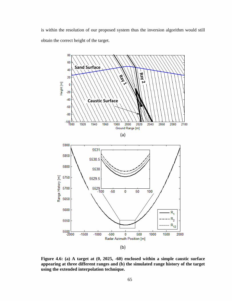
65

is within the resolution of our proposed system thus the inversion algorithm would still

obtain the correct height of the target.

(b)

(a)

Caustic Surface

Ray 1

Ray 2

Sand Surface

Figure 4.6: (a) A target at (0, 2025, -60) enclosed within a simple caustic surface

appearing at three different ranges and (b) the simulated range history of the target

using the extended interpolation technique.

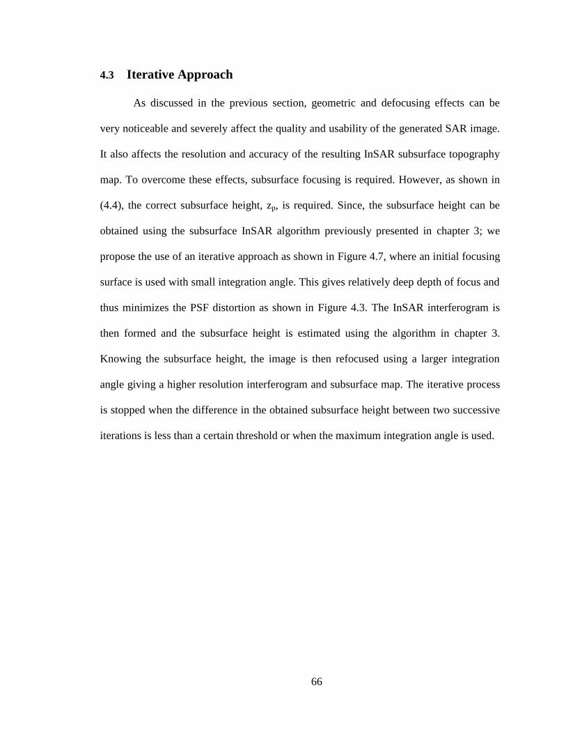
66

4.3 Iterative Approach

As discussed in the previous section, geometric and defocusing effects can be

very noticeable and severely affect the quality and usability of the generated SAR image.

It also affects the resolution and accuracy of the resulting InSAR subsurface topography

map. To overcome these effects, subsurface focusing is required. However, as shown in

(4.4), the correct subsurface height, zp, is required. Since, the subsurface height can be

obtained using the subsurface InSAR algorithm previously presented in chapter 3; we

propose the use of an iterative approach as shown in Figure 4.7, where an initial focusing

surface is used with small integration angle. This gives relatively deep depth of focus and

thus minimizes the PSF distortion as shown in Figure 4.3. The InSAR interferogram is

then formed and the subsurface height is estimated using the algorithm in chapter 3.

Knowing the subsurface height, the image is then refocused using a larger integration

angle giving a higher resolution interferogram and subsurface map. The iterative process

is stopped when the difference in the obtained subsurface height between two successive

iterations is less than a certain threshold or when the maximum integration angle is used.

67

Raw SAR Data

Conventional Focusing with Small Integration Angle

Application of the Subsurface Inversion Algorithm

Generation of the Doppler History using the Subsurface SAR Simulator

Refocusing Through the Sand Layer using Subsurface Focusing

Desired

Resolution

Achieved ?

End

Increase the Integration Angle

Yes

No

Figure 4.7: The proposed iterative scheme.

4.4 Simulation Results

The proposed iterative focusing approach was applied to two scenarios as shown

in Figure 4.8 and Figure 4.9. In Figure 4.8 (a) a grid of ideal point targets spaced by 20 m

along the azimuth and the ground range, placed on the surface of a cone is simulated

under a linear sand dune. The results of applying conventional focusing with 10o and 40

o

on the sand surface are shown in Figure 4.8 (c) and (d). We can see that small integration

angles yields relatively low resolution but the point targets responses do not show

noticeable dispersion as indicated in Figure 4.3 whereas using large integration angles

results in distorted response as expected. On the other hand, using the subsurface

focusing technique, we started by an image very similar to that of conventional focusing.

However, once the subsurface height is known and the focusing is performed at the

correct point targets heights, the integration angle can be increased to 40o without any

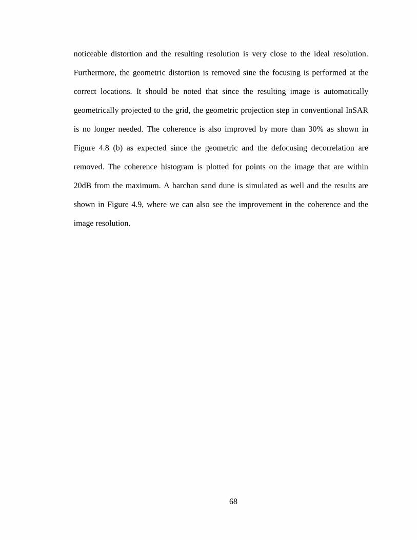
68

noticeable distortion and the resulting resolution is very close to the ideal resolution.

Furthermore, the geometric distortion is removed sine the focusing is performed at the

correct locations. It should be noted that since the resulting image is automatically

geometrically projected to the grid, the geometric projection step in conventional InSAR

is no longer needed. The coherence is also improved by more than 30% as shown in

Figure 4.8 (b) as expected since the geometric and the defocusing decorrelation are

removed. The coherence histogram is plotted for points on the image that are within

20dB from the maximum. A barchan sand dune is simulated as well and the results are

shown in Figure 4.9, where we can also see the improvement in the coherence and the

image resolution.

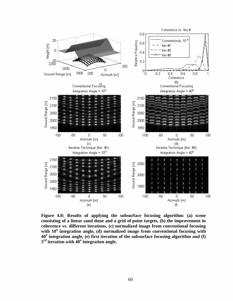
69

Figure 4.8: Results of applying the subsurface focusing algorithm: (a) scene

consisting of a linear sand dune and a grid of point targets, (b) the improvement in

coherence vs. different iterations, (c) normalized image from conventional focusing

with 10o integration angle, (d) normalized image from conventional focusing with

40o integration angle, (e) first iteration of the subsurface focusing algorithm and (f)

3rd

iteration with 40o integration angle.

a)

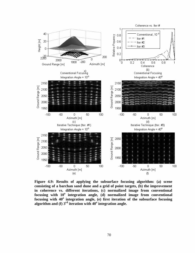
70

Figure 4.9: Results of applying the subsurface focusing algorithm: (a) scene

consisting of a barchan sand dune and a grid of point targets, (b) the improvement

in coherence vs. different iterations, (c) normalized image from conventional

focusing with 10o integration angle, (d) normalized image from conventional

focusing with 40o integration angle, (e) first iteration of the subsurface focusing

algorithm and (f) 3rd

iteration with 40o integration angle.

a)

71

4.5 Scaled Model Measurement Results

To verify the performance of the proposed algorithm, we used a scaled model in

the lab as described in Chapter 3. The resulting SAR image for one of the passes is shown

in Figure 4.10 (a). The coherence results over the sand covered area using conventional

focusing and using the proposed algorithm are shown in Figure 4.10 (b). The coherence

was estimated using 4x4 resolution cells. The improvement in coherence is due to the

correction for the geometric distortion and the improvement in the focusing which are not

very severe in this scenario due to the flat surface and the relatively shallow sand layer.

However, thicker sand layer or more complex top surface, the improvement in the

coherence is expected to be even more pronounced.

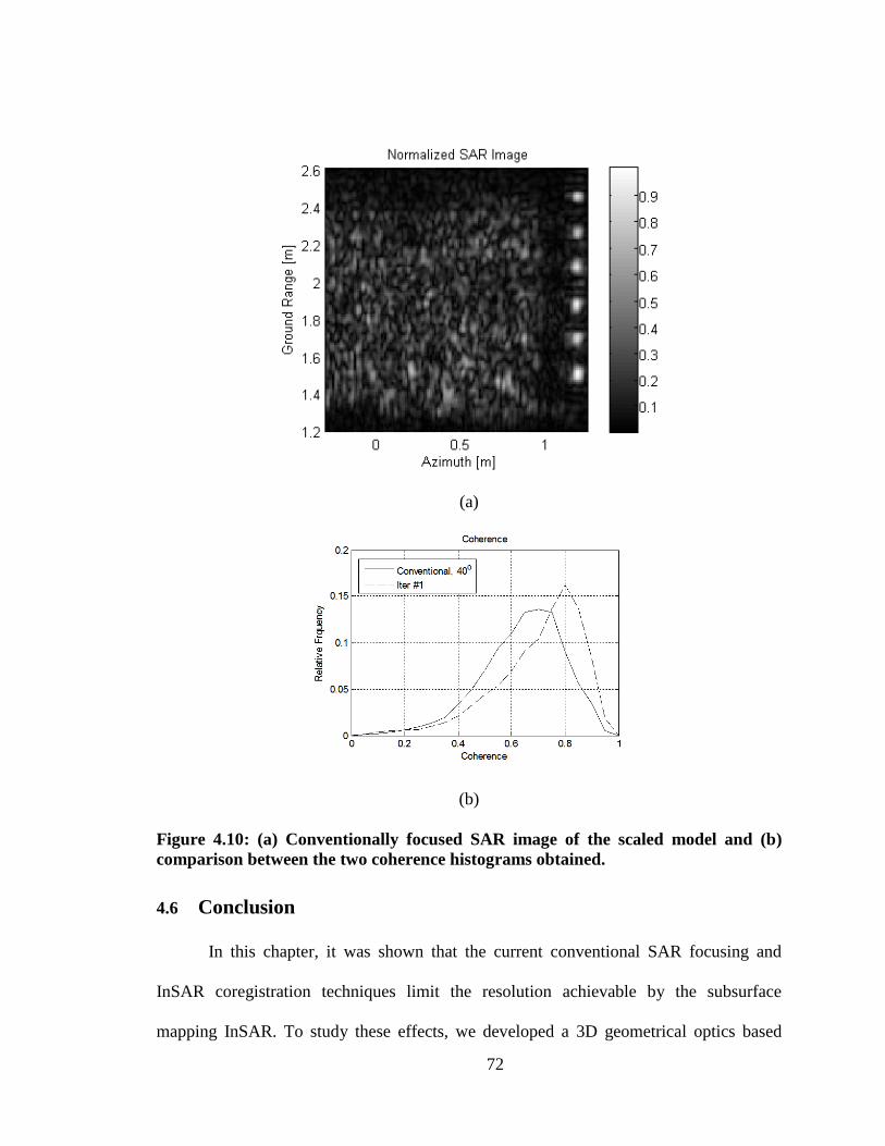
72

(a)

(b)

Figure 4.10: (a) Conventionally focused SAR image of the scaled model and (b)

comparison between the two coherence histograms obtained.

4.6 Conclusion

In this chapter, it was shown that the current conventional SAR focusing and

InSAR coregistration techniques limit the resolution achievable by the subsurface

mapping InSAR. To study these effects, we developed a 3D geometrical optics based

73

subsurface SAR simulator. Using the simulator, the two major types of artifacts are

shown to be defocusing and geometric distortion. Defocusing severely limits the image

resolution and geometric distortions limit its use in many applications. We then presented

an iterative approach that combines the subsurface inversion algorithm and the 3D

subsurface SAR simulator. The iterative approach is then applied to a simulated sample

scene and was shown to remove all the geometric artifacts and to provide much higher

resolution image. It was also experimentally verified using scaled model measurement.

The main drawback of the proposed technique is the computational requirements of the

subsurface SAR simulator and subsurface focusing. However, it can easily be parallelized

to enhance the speed.

74

Chapter 5

Linearly Polarized Ultra-Wideband Antennas

The previous three chapters dealt with the propagation modeling and inversion

parts of the subsurface topography estimation problem. The next three chapters deal with

a very important system implementation problem which is the radar antennas for this

system. The proposed subsurface topography estimation system requires an Ultra-

Wideband (UWB) antenna to be mounted on the plane for the low frequency InSAR

subsystem. The system also requires UWB antennas for the ground penetrating radars

that are used to find the subsurface heights at the ground control points (GCPs). These

antennas have to 1) operate at low frequencies (VHF) in order to penetrate through the

sand layer, 2) operate over a very large relative bandwidth in order to provide good

height resolution and 3) have compact size for mounting on the plane or on a vehicle. In

this chapter, the design of a number of compact linearly polarized UWB antennas for

these applications is presented. Incidentally, such antennas are also very useful in many

other applications such as see through wall radars and communications applications. The

antennas in the next chapters are scaled up in frequency so that they can be easily

measured in laboratory environment. The chapter begins with the background

information about UWB antennas and some of the standard designs then proceeds to the

first set of the newly developed antennas.

75

5.1 Background

5.1.1 Definitions

There are two commonly used definitions for UWB Antennas ( is the minimum

operating frequency of the antenna and is the highest operating frequency) [43], [44]:

1. The Defense Advanced Research Projects Agency (DARPA) Definition:

2. The Federal Communications Commission (FCC) Definition:

Or

In this thesis, most of the designed antennas have operating fractional bandwidths

from 67% to more than 120% and bandwidths in excess of 1 GHz, and thus both

definitions apply.

5.1.2 Design Issues

Unlike conventional narrowband antennas which operate over relatively narrow

bandwidths with (mostly) one mode of operation and relatively constant radiation

characteristics, UWB antennas operate over much wider bandwidths over which their

radiation characteristics can change drastically. There are four major performance metrics

for UWB antennas that are of interest for the applications considered in this thesis,

namely: (1) overall efficiency, (2) radiation pattern, (3) time domain performance and (4)

electrical size [45].

76

Overall efficiency is defined as the radiated power from the antenna divided by

the incident power at its terminal. It is related to the antenna matching as well as the

dielectric and metallic losses in the antenna. Some ultra-wideband antennas are

miniaturized using lossy elements. However, this usually leads to degraded noise

performance which limits their use in radars and high performance communication

systems thus such antennas are not considered in this thesis.

The radiation pattern is very important in radar antenna designs. Radar antennas

are designed such that they have low side lobes and large front-to-back ratios (ratio

between the radiated power in the forward direction to that in the backward direction).

This is because high side lobes cause the same target to be detected at different azimuth

positions in a radar image which affect the quality of the image whereas low front-to-

back ratio causes the operator and/or the mounting structure of the antenna to affect the

generated image.

The time domain performance of the antenna is extremely important in radar

and communication applications. This is because UWB radars and communication

systems transmit and receive very narrow pulses in the time domain (and is thus very

wide in the frequency domain). The antenna should not cause significant distortion to

these pulses; otherwise the performance of the systems can degrade drastically. For

example, if an antenna which has bad time domain performance is used in a radar system,

a single target can appear as multiple targets at different ranges from the radar and mask

weaker targets at other ranges. It can also cause significant bit errors in UWB

communication systems.

77

The antenna electrical size is defined as the antenna physical size divided by the

operating wavelength. For UWB antennas, due to the large bandwidth, the used

wavelength is usually the wavelength at the minimum operating frequency or,

equivalently, the maximum operating wavelength. The antenna size is required to be as

small as possible for several reasons.

1. Many UWB radar systems such as GPRs and see-through wall radars

operate at low frequencies in order to penetrate through moist soil and

lossy walls. For these radars, antennas are the limitation on the overall

system size. Thus, small antenna size is very important to reduce the

overall system size and weight. This is also very important for plane

mounted antennas for the InSAR system.

2. Some radars and communication systems use UWB arrays. From array

theory, it can be shown that if the separation between the elements in an

array is significantly larger than half the operating wavelength, grating

lobes appear. Grating lobes are very large side lobes that can cause severe

image artifacts in radars [45]. Grating lobes also greatly reduce the overall

gain of the array which can cause significant noise issues in

communication and radar systems. By reducing the antenna size, the

spacing between the antenna elements can be maintained to be less than

one half wavelengths over the operating bandwidth of the array.

3. Antenna size is also a limiting factor in many mobile communication

systems. By reducing the antenna size, significantly smaller UWB mobile

communication systems can be achieved.

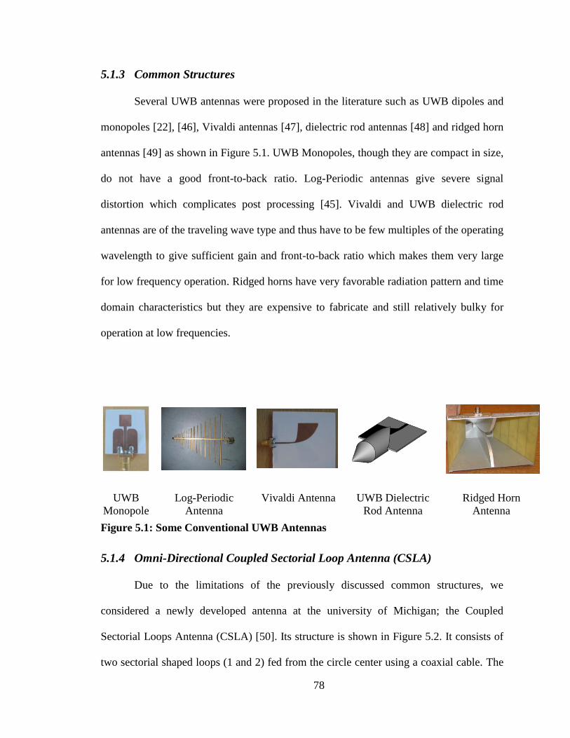
78

5.1.3 Common Structures

Several UWB antennas were proposed in the literature such as UWB dipoles and

monopoles [22], [46], Vivaldi antennas [47], dielectric rod antennas [48] and ridged horn

antennas [49] as shown in Figure 5.1. UWB Monopoles, though they are compact in size,

do not have a good front-to-back ratio. Log-Periodic antennas give severe signal

distortion which complicates post processing [45]. Vivaldi and UWB dielectric rod

antennas are of the traveling wave type and thus have to be few multiples of the operating

wavelength to give sufficient gain and front-to-back ratio which makes them very large

for low frequency operation. Ridged horns have very favorable radiation pattern and time

domain characteristics but they are expensive to fabricate and still relatively bulky for

operation at low frequencies.

UWB

Monopole

Log-Periodic

Antenna

Vivaldi Antenna

UWB Dielectric

Rod Antenna

Ridged Horn

Antenna

Figure 5.1: Some Conventional UWB Antennas

5.1.4 Omni-Directional Coupled Sectorial Loop Antenna (CSLA)

Due to the limitations of the previously discussed common structures, we

considered a newly developed antenna at the university of Michigan; the Coupled

Sectorial Loops Antenna (CSLA) [50]. Its structure is shown in Figure 5.2. It consists of

two sectorial shaped loops (1 and 2) fed from the circle center using a coaxial cable. The

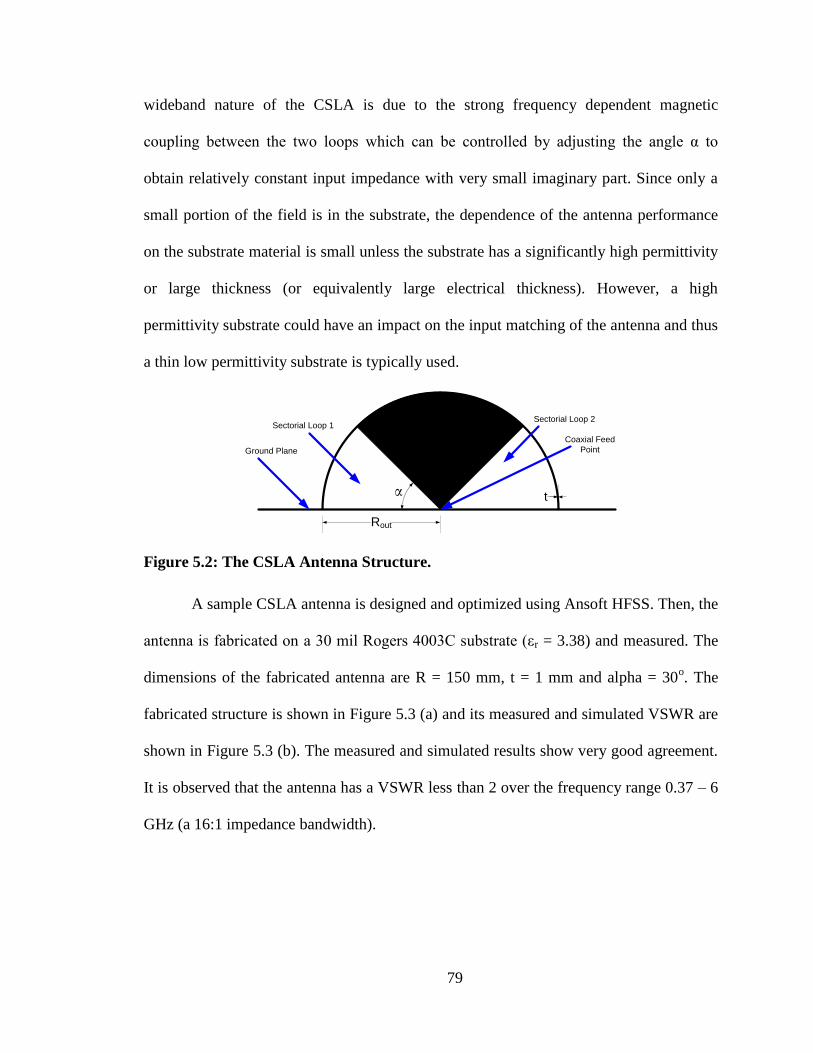
79

wideband nature of the CSLA is due to the strong frequency dependent magnetic

coupling between the two loops which can be controlled by adjusting the angle α to

obtain relatively constant input impedance with very small imaginary part. Since only a

small portion of the field is in the substrate, the dependence of the antenna performance

on the substrate material is small unless the substrate has a significantly high permittivity

or large thickness (or equivalently large electrical thickness). However, a high

permittivity substrate could have an impact on the input matching of the antenna and thus

a thin low permittivity substrate is typically used.

Sectorial Loop 1Sectorial Loop 2

Coaxial Feed

PointGround Plane

α

Rout

t

Figure 5.2: The CSLA Antenna Structure.

A sample CSLA antenna is designed and optimized using Ansoft HFSS. Then, the

antenna is fabricated on a 30 mil Rogers 4003C substrate (εr = 3.38) and measured. The

dimensions of the fabricated antenna are R = 150 mm, t = 1 mm and alpha = 30o. The

fabricated structure is shown in Figure 5.3 (a) and its measured and simulated VSWR are

shown in Figure 5.3 (b). The measured and simulated results show very good agreement.

It is observed that the antenna has a VSWR less than 2 over the frequency range 0.37 – 6

GHz (a 16:1 impedance bandwidth).

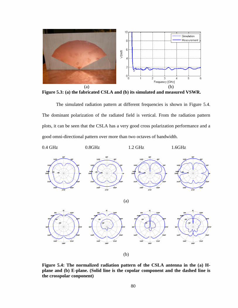
80

(a) (b)

Figure 5.3: (a) the fabricated CSLA and (b) its simulated and measured VSWR.

The simulated radiation pattern at different frequencies is shown in Figure 5.4.

The dominant polarization of the radiated field is vertical. From the radiation pattern

plots, it can be seen that the CSLA has a very good cross polarization performance and a

good omni-directional pattern over more than two octaves of bandwidth.

0.4 GHz 0.8GHz 1.2 GHz 1.6GHz

(a)

(b)

Figure 5.4: The normalized radiation pattern of the CSLA antenna in the (a) H-

plane and (b) E-plane. (Solid line is the copolar component and the dashed line is

the crosspolar conponent)

-40-200dB

0

30

60

90

120

150

180

210

240

270

300

330

-40-200dB

0

30

60

90

120

150

180

210

240

270

300

330

-40-200dB

0

30

60

90

120

150

180

210

240

270

300

330

-40-200dB

0

30

60

90

120

150

180

210

240

270

300

330

-40

-20

0dB

0

30

60

90

120

150

180

210

240

270

300

330

-40

-20

0dB

0

30

60

90

120

150

180

210

240

270

300

330

-40

-20

0dB

0

30

60

90

120

150

180

210

240

270

300

330

-40

-20

0dB

0

30

60

90

120

150

180

210

240

270

300

330

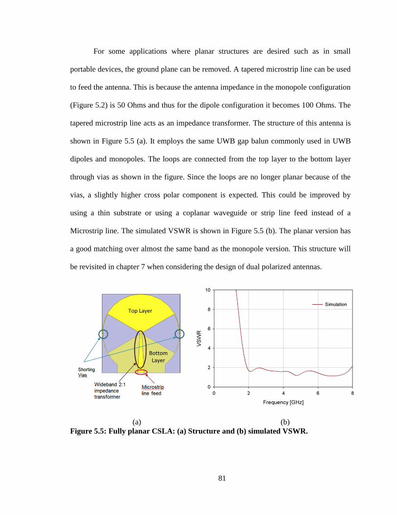
81

For some applications where planar structures are desired such as in small

portable devices, the ground plane can be removed. A tapered microstrip line can be used

to feed the antenna. This is because the antenna impedance in the monopole configuration

(Figure 5.2) is 50 Ohms and thus for the dipole configuration it becomes 100 Ohms. The

tapered microstrip line acts as an impedance transformer. The structure of this antenna is

shown in Figure 5.5 (a). It employs the same UWB gap balun commonly used in UWB

dipoles and monopoles. The loops are connected from the top layer to the bottom layer

through vias as shown in the figure. Since the loops are no longer planar because of the

vias, a slightly higher cross polar component is expected. This could be improved by

using a thin substrate or using a coplanar waveguide or strip line feed instead of a

Microstrip line. The simulated VSWR is shown in Figure 5.5 (b). The planar version has

a good matching over almost the same band as the monopole version. This structure will

be revisited in chapter 7 when considering the design of dual polarized antennas.

Top Layer

Bottom Layer

(a) (b)

Figure 5.5: Fully planar CSLA: (a) Structure and (b) simulated VSWR.

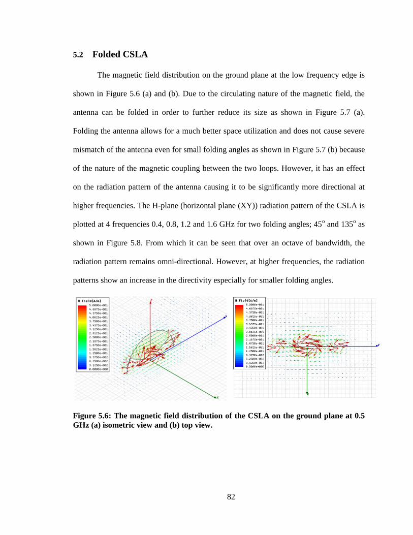
82

5.2 Folded CSLA

The magnetic field distribution on the ground plane at the low frequency edge is

shown in Figure 5.6 (a) and (b). Due to the circulating nature of the magnetic field, the

antenna can be folded in order to further reduce its size as shown in Figure 5.7 (a).

Folding the antenna allows for a much better space utilization and does not cause severe

mismatch of the antenna even for small folding angles as shown in Figure 5.7 (b) because

of the nature of the magnetic coupling between the two loops. However, it has an effect

on the radiation pattern of the antenna causing it to be significantly more directional at

higher frequencies. The H-plane (horizontal plane (XY)) radiation pattern of the CSLA is

plotted at 4 frequencies 0.4, 0.8, 1.2 and 1.6 GHz for two folding angles; 45o and 135

o as

shown in Figure 5.8. From which it can be seen that over an octave of bandwidth, the

radiation pattern remains omni-directional. However, at higher frequencies, the radiation

patterns show an increase in the directivity especially for smaller folding angles.

Figure 5.6: The magnetic field distribution of the CSLA on the ground plane at 0.5

GHz (a) isometric view and (b) top view.

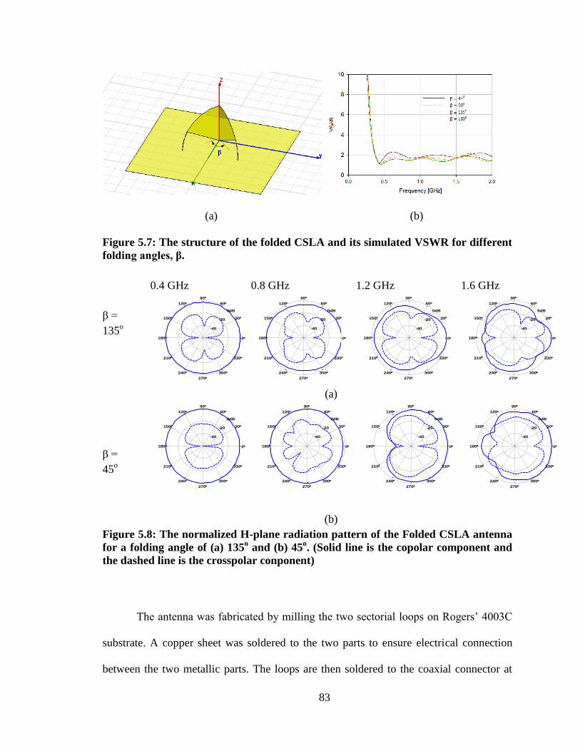
83

β

(a) (b)

Figure 5.7: The structure of the folded CSLA and its simulated VSWR for different

folding angles, β.

0.4 GHz 0.8 GHz 1.2 GHz 1.6 GHz

β =

135o

(a)

β =

45o

(b)

Figure 5.8: The normalized H-plane radiation pattern of the Folded CSLA antenna

for a folding angle of (a) 135o and (b) 45

o. (Solid line is the copolar component and

the dashed line is the crosspolar conponent)

The antenna was fabricated by milling the two sectorial loops on Rogers’ 4003C

substrate. A copper sheet was soldered to the two parts to ensure electrical connection

between the two metallic parts. The loops are then soldered to the coaxial connector at

-40

-20

0dB

0

30

60

90

120

150

180

210

240

270

300

330

-40

-20

0dB

0

30

60

90

120

150

180

210

240

270

300

330

-40

-20

0dB

0

30

60

90

120

150

180

210

240

270

300

330

-40

-20

0dB

0

30

60

90

120

150

180

210

240

270

300

330

-40

-20

0dB

0

30

60

90

120

150

180

210

240

270

300

330

-40

-20

0dB

0

30

60

90

120

150

180

210

240

270

300

330

-40

-20

0dB

0

30

60

90

120

150

180

210

240

270

300

330

-40

-20

0dB

0

30

60

90

120

150

180

210

240

270

300

330

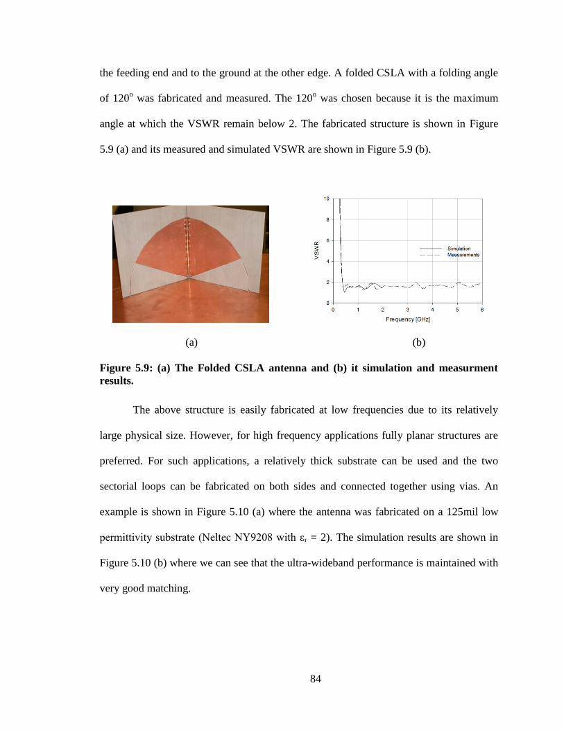
84

the feeding end and to the ground at the other edge. A folded CSLA with a folding angle

of 120o was fabricated and measured. The 120

o was chosen because it is the maximum

angle at which the VSWR remain below 2. The fabricated structure is shown in Figure

5.9 (a) and its measured and simulated VSWR are shown in Figure 5.9 (b).

(a) (b)

Figure 5.9: (a) The Folded CSLA antenna and (b) it simulation and measurment

results.

The above structure is easily fabricated at low frequencies due to its relatively

large physical size. However, for high frequency applications fully planar structures are

preferred. For such applications, a relatively thick substrate can be used and the two

sectorial loops can be fabricated on both sides and connected together using vias. An

example is shown in Figure 5.10 (a) where the antenna was fabricated on a 125mil low

permittivity substrate (Neltec NY9208 with εr = 2). The simulation results are shown in

Figure 5.10 (b) where we can see that the ultra-wideband performance is maintained with

very good matching.

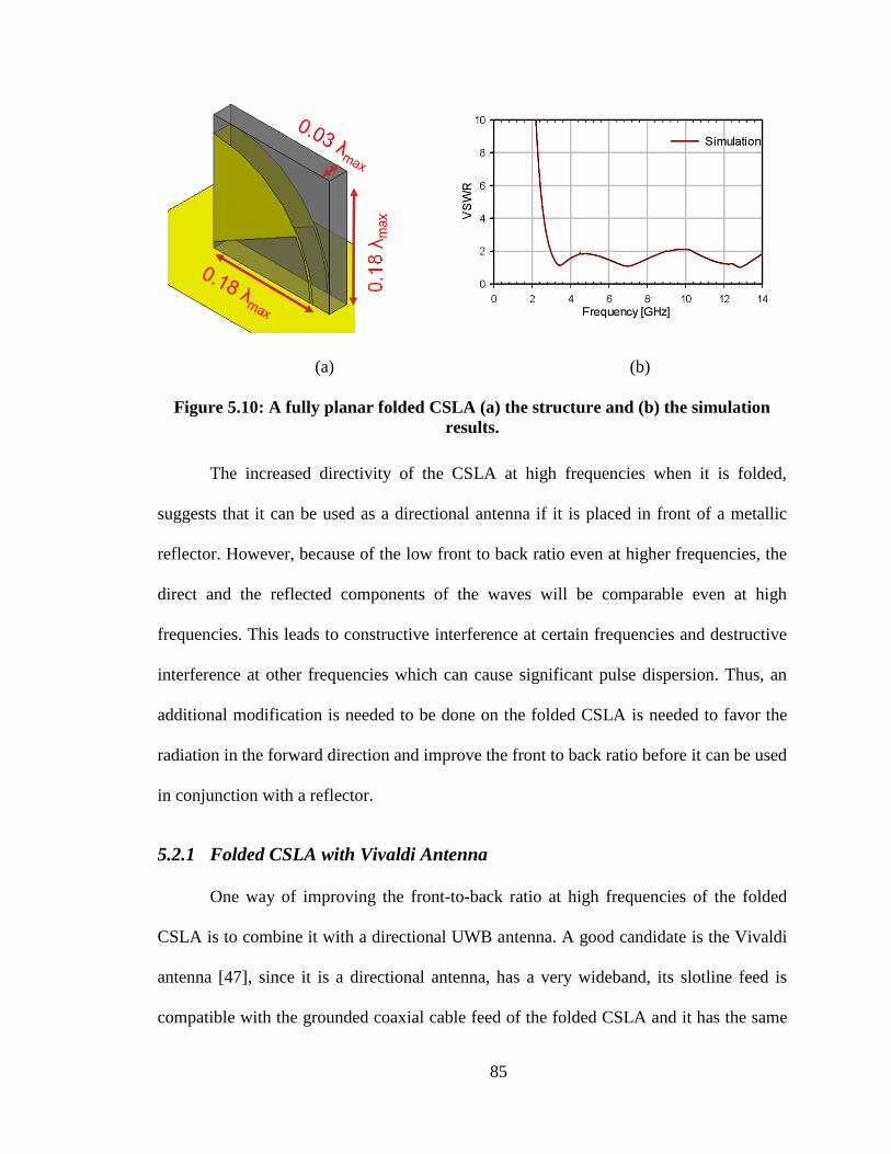
85

(a) (b)

Figure 5.10: A fully planar folded CSLA (a) the structure and (b) the simulation

results.

The increased directivity of the CSLA at high frequencies when it is folded,

suggests that it can be used as a directional antenna if it is placed in front of a metallic

reflector. However, because of the low front to back ratio even at higher frequencies, the

direct and the reflected components of the waves will be comparable even at high

frequencies. This leads to constructive interference at certain frequencies and destructive

interference at other frequencies which can cause significant pulse dispersion. Thus, an

additional modification is needed to be done on the folded CSLA is needed to favor the

radiation in the forward direction and improve the front to back ratio before it can be used

in conjunction with a reflector.

5.2.1 Folded CSLA with Vivaldi Antenna

One way of improving the front-to-back ratio at high frequencies of the folded

CSLA is to combine it with a directional UWB antenna. A good candidate is the Vivaldi

antenna [47], since it is a directional antenna, has a very wideband, its slotline feed is

compatible with the grounded coaxial cable feed of the folded CSLA and it has the same

86

vertical polarization as the CSLA. Vivaldi antennas can have several taper shapes, such

as exponential, elliptical or even circular. Exponential and elliptical tapers are usually

preferred in most designs since they allow the antenna to be well matched to its feeding

slot line. However, this is the case for a Vivaldi that is fed alone. When it is fed in

parallel with a CSLA, we found that circular taper gives better overall radiation pattern

performance and good matching performance since the taper shape affects the magnetic

coupling between the loops of the CSLA and thus the input matching of the antenna.

Based on that, a 120o folded CSLA combined with a Vivaldi with circular shaped inner

and outer tapers was designed as shown in Figure 5.11 (a). The outer circular taper of the

Vivaldi was found to improve the radiation pattern stability with frequency while not

significantly affecting the matching. The combined structure has an improved matching

compared to the folded CSLA at the low frequencies and its peak directivity is higher by

about 3dB as shown in Figure 5.11 (b) and (c). The fabricated structure together with its

measured and simulated VSWR are shown in Figure 5.12 (a) and (b) respectively.

Folded CSLA

Circularly tapered Vivaldi

(a) (b) (c)

Figure 5.11: (a) The combined Folded CSLA and the Vivaldi Antenna, (b)

comparison between the simulated directivity of the two antennas and (c) the H-

plane radiation pattern of the combined antenna at different frequencies.

87

(a) (b)

Figure 5.12: (a) The structure of the Vivaldi-CSLA antenna and (b) its simulated

and measured VSWR.

From the simulated radiation patterns of the antenna shown in Figure 5.11 (d), it

can be seen that the antenna has a more directive radiation at higher frequencies as

compared to the folded CSLA. It also has a better front to back ratio, which means that a

metallic reflector can now be used without causing severe variations in the gain at higher

frequencies. Having a good gain at low frequencies is very important in many UWB

radar applications; especially for through-wall imaging applications where most of the

signal penetration occurs at the low frequency portion. The low directivity is a physical

limit because of the small electrical dimensions of the CSLA. The reflector design for

UWB operation is discussed briefly in the next section.

5.2.2 Reflector Design for UWB Operation

The use of flat or shaped reflectors for increasing the directivity of antennas is a

very mature topic and several types of reflectors were presented in the literature such as

the corner, parabolic and paraboloidal reflectors. Typically, reflectors are placed

relatively far from the antenna in order not to severely affect its input impedance. For

UWB radar applications, placing the reflector too far from the antenna can cause severe

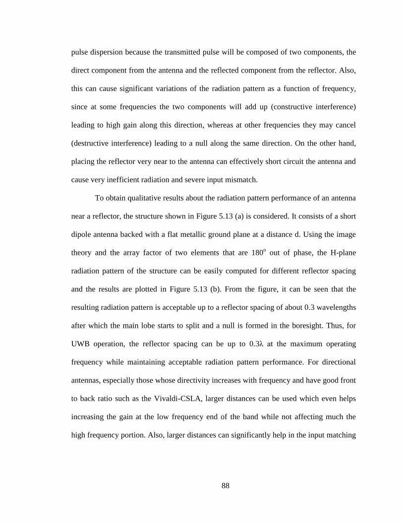
88

pulse dispersion because the transmitted pulse will be composed of two components, the

direct component from the antenna and the reflected component from the reflector. Also,

this can cause significant variations of the radiation pattern as a function of frequency,

since at some frequencies the two components will add up (constructive interference)

leading to high gain along this direction, whereas at other frequencies they may cancel

(destructive interference) leading to a null along the same direction. On the other hand,

placing the reflector very near to the antenna can effectively short circuit the antenna and

cause very inefficient radiation and severe input mismatch.

To obtain qualitative results about the radiation pattern performance of an antenna

near a reflector, the structure shown in Figure 5.13 (a) is considered. It consists of a short

dipole antenna backed with a flat metallic ground plane at a distance d. Using the image

theory and the array factor of two elements that are 180o out of phase, the H-plane

radiation pattern of the structure can be easily computed for different reflector spacing

and the results are plotted in Figure 5.13 (b). From the figure, it can be seen that the

resulting radiation pattern is acceptable up to a reflector spacing of about 0.3 wavelengths

after which the main lobe starts to split and a null is formed in the boresight. Thus, for

UWB operation, the reflector spacing can be up to 0.3λ at the maximum operating

frequency while maintaining acceptable radiation pattern performance. For directional

antennas, especially those whose directivity increases with frequency and have good front

to back ratio such as the Vivaldi-CSLA, larger distances can be used which even helps

increasing the gain at the low frequency end of the band while not affecting much the

high frequency portion. Also, larger distances can significantly help in the input matching

89

at lower frequencies. The placement of a reflector in the back of the Vivaldi-CSLA is

presented in the next section.

I

Dipole

Metal

Reflector

d

(a) (b)

Figure 5.13: (a) A dipole parallel to a flat ground plane and (b) the resulting H-

plane radiation pattern for different reflector spacings.

5.2.3 Vivaldi-CSLA Antenna with Reflector

5.2.3.1 Flat Reflector

Based on the analysis presented in the previous section, we investigated the

placement of a reflector near the backside of the Vivaldi-CSLA as shown in Figure 5.14

(a). This is expected to significantly improve the directivity at low frequencies without

adversely affecting the radiation pattern at higher frequencies since the antenna already

has good directivity at high frequencies. It is also expected to further improve the front to

back ratio over most of the band. However, placing a reflector very near to the coupled

loops would severely impact the magnetic coupling between them and affect the low

frequency end of operation. The simulation results of the peak directivity and the input

VSWR are shown in Figure 5.14 (c) and (d) respectively. These figures show that the

minimum operating frequency is strongly dependent on the placement of the reflector.

90

However, placing the reflector far from the antenna, impacts the directivity at higher

frequencies.

Reflector

d

(a)

(b) (c)

Figure 5.14: (a) The Vivaldi-CSLA placed in front of a flat reflector and the

simulated (b) peak directivity of the Vivaldi-CSLA with a planar reflector and (c)

the VSWR for different reflector spacing, d.

5.2.3.2 Corner Reflector

5.2.3.2.1 Structure

As seen from the directivity vs. frequency plots, placing a flat back reflector,

significantly improves the low frequency directivity as expected (the directivity increased

by about 4dB compared to the no-reflector case). However, it caused the radiation pattern

and the directivity to have undesired fast variations at high frequencies. Thus, in order to

further improve the antenna performance, a corner reflector is used instead of a simple

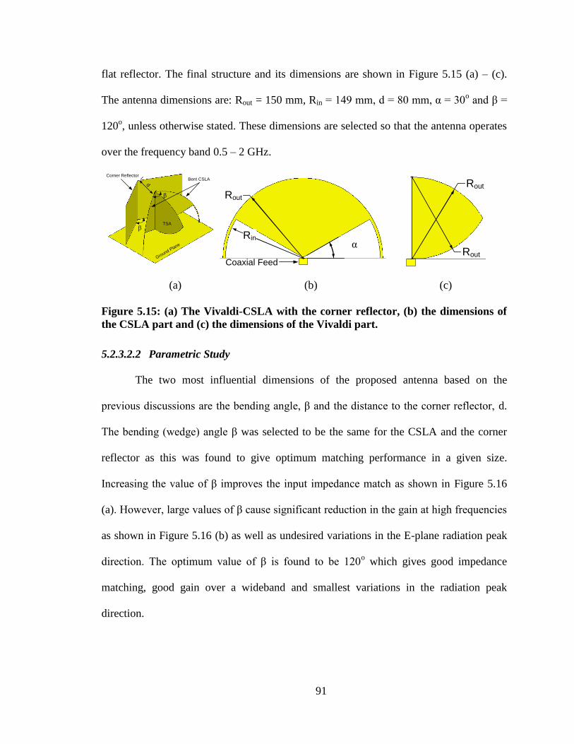
91

flat reflector. The final structure and its dimensions are shown in Figure 5.15 (a) – (c).

The antenna dimensions are: Rout = 150 mm, Rin = 149 mm, d = 80 mm, α = 30o and β =

120o, unless otherwise stated. These dimensions are selected so that the antenna operates

over the frequency band 0.5 – 2 GHz.

Ground Plane

Corner Reflector

TSA

Bent CSLA

β

d

β

Rin

Rout

α

Coaxial Feed

Rout

Rout

(a) (b) (c)

Figure 5.15: (a) The Vivaldi-CSLA with the corner reflector, (b) the dimensions of

the CSLA part and (c) the dimensions of the Vivaldi part.

5.2.3.2.2 Parametric Study

The two most influential dimensions of the proposed antenna based on the

previous discussions are the bending angle, β and the distance to the corner reflector, d.

The bending (wedge) angle β was selected to be the same for the CSLA and the corner

reflector as this was found to give optimum matching performance in a given size.

Increasing the value of β improves the input impedance match as shown in Figure 5.16

(a). However, large values of β cause significant reduction in the gain at high frequencies

as shown in Figure 5.16 (b) as well as undesired variations in the E-plane radiation peak

direction. The optimum value of β is found to be 120o which gives good impedance

matching, good gain over a wideband and smallest variations in the radiation peak

direction.

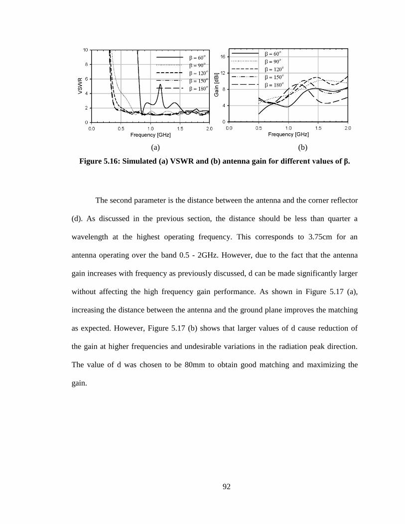
92

(a) (b)

Figure 5.16: Simulated (a) VSWR and (b) antenna gain for different values of β.

The second parameter is the distance between the antenna and the corner reflector

(d). As discussed in the previous section, the distance should be less than quarter a

wavelength at the highest operating frequency. This corresponds to 3.75cm for an

antenna operating over the band 0.5 - 2GHz. However, due to the fact that the antenna

gain increases with frequency as previously discussed, d can be made significantly larger

without affecting the high frequency gain performance. As shown in Figure 5.17 (a),

increasing the distance between the antenna and the ground plane improves the matching

as expected. However, Figure 5.17 (b) shows that larger values of d cause reduction of

the gain at higher frequencies and undesirable variations in the radiation peak direction.

The value of d was chosen to be 80mm to obtain good matching and maximizing the

gain.

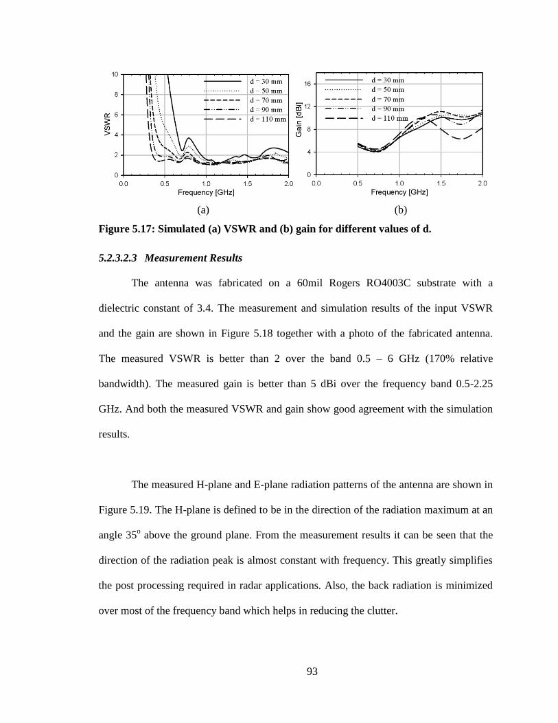
93

(a) (b)

Figure 5.17: Simulated (a) VSWR and (b) gain for different values of d.

5.2.3.2.3 Measurement Results

The antenna was fabricated on a 60mil Rogers RO4003C substrate with a

dielectric constant of 3.4. The measurement and simulation results of the input VSWR

and the gain are shown in Figure 5.18 together with a photo of the fabricated antenna.

The measured VSWR is better than 2 over the band 0.5 – 6 GHz (170% relative

bandwidth). The measured gain is better than 5 dBi over the frequency band 0.5-2.25

GHz. And both the measured VSWR and gain show good agreement with the simulation

results.

The measured H-plane and E-plane radiation patterns of the antenna are shown in

Figure 5.19. The H-plane is defined to be in the direction of the radiation maximum at an

angle 35o above the ground plane. From the measurement results it can be seen that the

direction of the radiation peak is almost constant with frequency. This greatly simplifies

the post processing required in radar applications. Also, the back radiation is minimized

over most of the frequency band which helps in reducing the clutter.

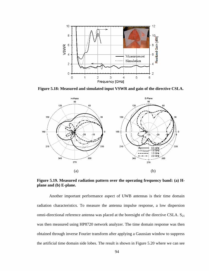
94

Figure 5.18: Measured and simulated input VSWR and gain of the directive CSLA.

(a) (b)

Figure 5.19. Measured radiation pattern over the operating frequency band: (a) H-

plane and (b) E-plane.

Another important performance aspect of UWB antennas is their time domain

radiation characteristics. To measure the antenna impulse response, a low dispersion

omni-directional reference antenna was placed at the boresight of the directive CSLA. S21

was then measured using HP8720 network analyzer. The time domain response was then

obtained through inverse Fourier transform after applying a Gaussian window to suppress

the artificial time domain side lobes. The result is shown in Figure 5.20 where we can see

95

that there is slight pulse widening due to the time delay between the direct ray and

reflected ray from the corner reflector. This corresponds to small loss in the range

resolution for radar application. However the time domain side lobe levels are below

20dB and there is no apparent ringing in the time domain response. The measurements

were not performed in the anechoic chamber and thus some multiple reflections due to

nearby objects appear in the time domain as shown in the figure. The multiple reflection

effects are reduced when using the directive CSLA compared to the reference antenna

due to the more directive radiation pattern of the directive CSLA.

A size comparison between the proposed antenna and a standard ridged horn is

shown in Figure 5.21. The proposed antenna size is almost one-eighth the size of the

ridged horn while having comparable gain. The proposed antenna is also easily fabricated

using PCB technology and does not require expensive high tolerance CNC machining

and assembly that are required for the fabrication of ridged horn antennas. However, its

operating bandwidth is only 4.5:1 compared to 18:1 of the ridged horn. But, for most

radar applications, 4:1 bandwidth provides sufficient resolution with reasonable system

and postprocessing complexity.

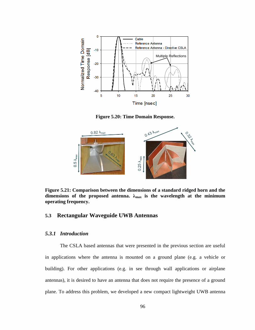
96

Multiple Reflections

Figure 5.20: Time Domain Response.

Figure 5.21: Comparison between the dimensions of a standard ridged horn and the

dimensions of the proposed antenna. λmax is the wavelength at the minimum

operating frequency.

5.3 Rectangular Waveguide UWB Antennas

5.3.1 Introduction

The CSLA based antennas that were presented in the previous section are useful

in applications where the antenna is mounted on a ground plane (e.g. a vehicle or

building). For other applications (e.g. in see through wall applications or airplane

antennas), it is desired to have an antenna that does not require the presence of a ground

plane. To address this problem, we developed a new compact lightweight UWB antenna

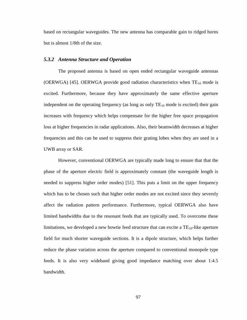
97

based on rectangular waveguides. The new antenna has comparable gain to ridged horns

but is almost 1/8th of the size.

5.3.2 Antenna Structure and Operation

The proposed antenna is based on open ended rectangular waveguide antennas

(OERWGA) [45]. OERWGA provide good radiation characteristics when TE10 mode is

excited. Furthermore, because they have approximately the same effective aperture

independent on the operating frequency (as long as only TE10 mode is excited) their gain

increases with frequency which helps compensate for the higher free space propagation

loss at higher frequencies in radar applications. Also, their beamwidth decreases at higher

frequencies and this can be used to suppress their grating lobes when they are used in a

UWB array or SAR.

However, conventional OERWGA are typically made long to ensure that that the

phase of the aperture electric field is approximately constant (the waveguide length is

needed to suppress higher order modes) [51]. This puts a limit on the upper frequency

which has to be chosen such that higher order modes are not excited since they severely

affect the radiation pattern performance. Furthermore, typical OERWGA also have

limited bandwidths due to the resonant feeds that are typically used. To overcome these

limitations, we developed a new bowtie feed structure that can excite a TE10-like aperture

field for much shorter waveguide sections. It is a dipole structure, which helps further

reduce the phase variation across the aperture compared to conventional monopole type

feeds. It is also very wideband giving good impedance matching over about 1:4.5

bandwidth.

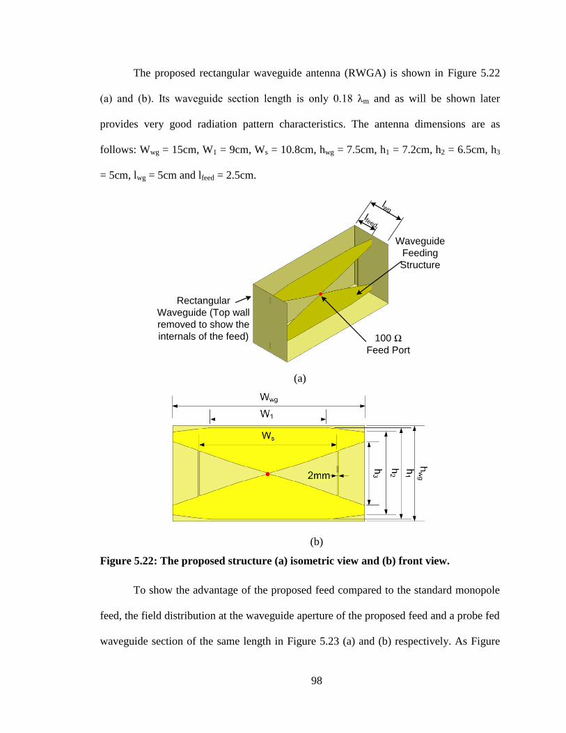
98

The proposed rectangular waveguide antenna (RWGA) is shown in Figure 5.22

(a) and (b). Its waveguide section length is only 0.18 λm and as will be shown later

provides very good radiation pattern characteristics. The antenna dimensions are as

follows: Wwg = 15cm, W1 = 9cm, Ws = 10.8cm, hwg = 7.5cm, h1 = 7.2cm, h2 = 6.5cm, h3

= 5cm, lwg = 5cm and lfeed = 2.5cm.

Rectangular

Waveguide (Top wall

removed to show the

internals of the feed)

Waveguide

Feeding

Structure

lfeed

lwg

100 Ω

Feed Port

(a)

(b)

Figure 5.22: The proposed structure (a) isometric view and (b) front view.

To show the advantage of the proposed feed compared to the standard monopole

feed, the field distribution at the waveguide aperture of the proposed feed and a probe fed

waveguide section of the same length in Figure 5.23 (a) and (b) respectively. As Figure

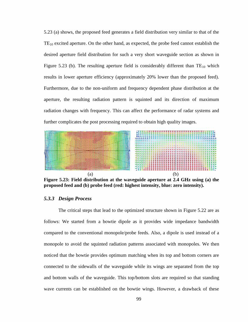
99

5.23 (a) shows, the proposed feed generates a field distribution very similar to that of the

TE10 excited aperture. On the other hand, as expected, the probe feed cannot establish the

desired aperture field distribution for such a very short waveguide section as shown in

Figure 5.23 (b). The resulting aperture field is considerably different than TE10 which

results in lower aperture efficiency (approximately 20% lower than the proposed feed).

Furthermore, due to the non-uniform and frequency dependent phase distribution at the

aperture, the resulting radiation pattern is squinted and its direction of maximum

radiation changes with frequency. This can affect the performance of radar systems and

further complicates the post processing required to obtain high quality images.

(a) (b)

Figure 5.23: Field distribution at the waveguide aperture at 2.4 GHz using (a) the

proposed feed and (b) probe feed (red: highest intensity, blue: zero intensity).

5.3.3 Design Process

The critical steps that lead to the optimized structure shown in Figure 5.22 are as

follows: We started from a bowtie dipole as it provides wide impedance bandwidth

compared to the conventional monopole/probe feeds. Also, a dipole is used instead of a

monopole to avoid the squinted radiation patterns associated with monopoles. We then

noticed that the bowtie provides optimum matching when its top and bottom corners are

connected to the sidewalls of the waveguide while its wings are separated from the top

and bottom walls of the waveguide. This top/bottom slots are required so that standing

wave currents can be established on the bowtie wings. However, a drawback of these

100

slots is that they create an unwanted resonance in the middle of the operating band. This

resonance is related to the third resonance of these slots and it was suppressed using the

shorting lines between the wings as shown in Figure 5.22 (b) thus reaching the final

structure.

Two of the important tuning parameters of the antenna will be discussed. The first

is h1 which controls the capacitive coupling between the bowtie and the waveguide

through the top/bottom slot widths. As shown in the simulation results in Figure 5.24 (a),

reducing h1 (increasing the slot width) helps in improving the matching but it also

increases the minimum operating frequency which increases the antenna size for a given

frequency band of operation and limits the resulting bandwidth. For optimum matching at

smallest antenna size, h1 was set to 7.2cm.

On the other hand, the top/bottom slots, even though they greatly help the

matching, they also create a resonance in the band near their odd resonance at around

2.95 GHz as shown in Figure 5.25. To remove this resonance, we added a shorting line

between the two wings as shown in Figure 5.22. By adjusting the separation Ws, we can

adjust the two resonances to cancel each other as shown in Figure 5.24 (b).

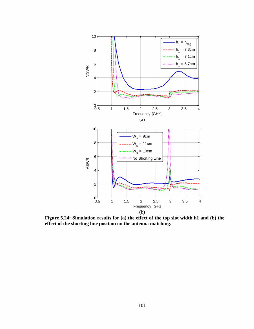
101

(a)

(b)

Figure 5.24: Simulation results for (a) the effect of the top slot width h1 and (b) the

effect of the shorting line position on the antenna matching.

0.5 1 1.5 2 2.5 3 3.5 40

2

4

6

8

10

Frequency [GHz]

VS

WR

h1 = h

w g

h1 = 7.3cm

h1 = 7.1cm

h1 = 6.7cm

0.5 1 1.5 2 2.5 3 3.5 40

2

4

6

8

10

Frequency [GHz]

VS

WR

Ws = 9cm

Ws = 11cm

Ws = 13cm

No Shorting Line

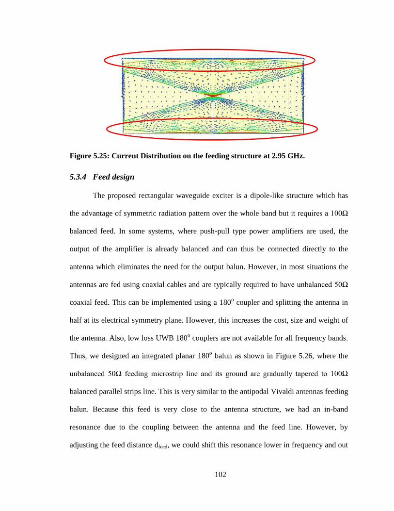
102

Figure 5.25: Current Distribution on the feeding structure at 2.95 GHz.

5.3.4 Feed design

The proposed rectangular waveguide exciter is a dipole-like structure which has

the advantage of symmetric radiation pattern over the whole band but it requires a 100Ω

balanced feed. In some systems, where push-pull type power amplifiers are used, the

output of the amplifier is already balanced and can thus be connected directly to the

antenna which eliminates the need for the output balun. However, in most situations the

antennas are fed using coaxial cables and are typically required to have unbalanced 50Ω

coaxial feed. This can be implemented using a 180o coupler and splitting the antenna in

half at its electrical symmetry plane. However, this increases the cost, size and weight of

the antenna. Also, low loss UWB 180o couplers are not available for all frequency bands.

Thus, we designed an integrated planar 180o balun as shown in Figure 5.26, where the

unbalanced 50Ω feeding microstrip line and its ground are gradually tapered to 100Ω

balanced parallel strips line. This is very similar to the antipodal Vivaldi antennas feeding

balun. Because this feed is very close to the antenna structure, we had an in-band

resonance due to the coupling between the antenna and the feed line. However, by

adjusting the feed distance dfeed, we could shift this resonance lower in frequency and out

103

of band. The loss of this feed was measured using a back-to-back junction and was found

to be less than 0.5dB over 1-5GHz. The microstrip line is linearly tapered from

to . The ground was exponentially tapered from

to according to the

equation:

(5.1)

Where:

(

)

(5.2)

and is the distance from the coaxial feed position (varies from 0 to

). The balun dimensions are given in Table 5.1.

30mil Rogers 4003C

Substrate

Feed Coaxial

Cable

MS line with

tapered ground

d feed

(a) (b)

Figure 5.26: The used balun for feeding the bowtie fed RWGA: (a) A cross section of

the RWGA at its electrical symmetry plane to show the feeding structure and (b) the

balun dimensions.

Table 5.1: Integrated microstrip balun dimensions.

Parameter

dw dfeed

Value 250 mm 1 mm 1.9 mm 15 mm 18 mm 109 mm

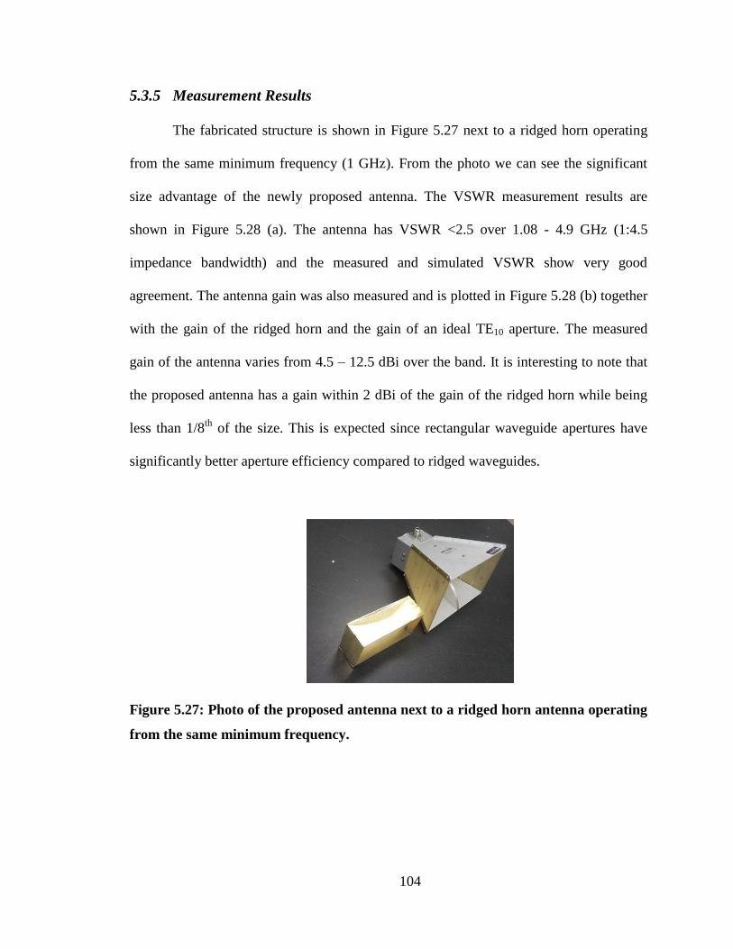
104

5.3.5 Measurement Results

The fabricated structure is shown in Figure 5.27 next to a ridged horn operating

from the same minimum frequency (1 GHz). From the photo we can see the significant

size advantage of the newly proposed antenna. The VSWR measurement results are

shown in Figure 5.28 (a). The antenna has VSWR <2.5 over 1.08 - 4.9 GHz (1:4.5

impedance bandwidth) and the measured and simulated VSWR show very good

agreement. The antenna gain was also measured and is plotted in Figure 5.28 (b) together

with the gain of the ridged horn and the gain of an ideal TE10 aperture. The measured

gain of the antenna varies from 4.5 – 12.5 dBi over the band. It is interesting to note that

the proposed antenna has a gain within 2 dBi of the gain of the ridged horn while being

less than 1/8th

of the size. This is expected since rectangular waveguide apertures have

significantly better aperture efficiency compared to ridged waveguides.

Figure 5.27: Photo of the proposed antenna next to a ridged horn antenna operating

from the same minimum frequency.

105

(a) (b)

Figure 5.28: (a) The measured and simulated VSWR of the proposed antenna and

(b) the measured and simulated gain compared to the gain of the ridged horn and

that of an ideal TE10 aperture.

The radiation pattern of the antenna was measured in the anechoic chamber and

the results are shown in Figure 5.29 (a) and (b) together with the simulation results. We

can see excellent agreement between the simulation and measurement results. The

radiation pattern had low side lobe levels up to about 3.5 GHz. These side lobes are

mainly due to the larger phase variations across the aperture at higher frequencies.

0 1 2 3 4 50

2

4

6

8

10

Frequency [GHz]

VS

WR

Simulation

Measurements

0.5 1 1.5 2 2.5 3 3.50

2

4

6

8

10

12

Frequency [GHz]

Gain

[dB

i]

Proposed Antenna

Ridged Horn Gain

Ideal TE10 aperture

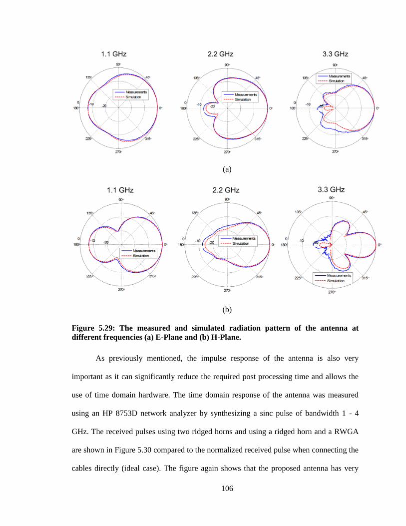
106

(a)

(b)

Figure 5.29: The measured and simulated radiation pattern of the antenna at

different frequencies (a) E-Plane and (b) H-Plane.

As previously mentioned, the impulse response of the antenna is also very

important as it can significantly reduce the required post processing time and allows the

use of time domain hardware. The time domain response of the antenna was measured

using an HP 8753D network analyzer by synthesizing a sinc pulse of bandwidth 1 - 4

GHz. The received pulses using two ridged horns and using a ridged horn and a RWGA

are shown in Figure 5.30 compared to the normalized received pulse when connecting the

cables directly (ideal case). The figure again shows that the proposed antenna has very

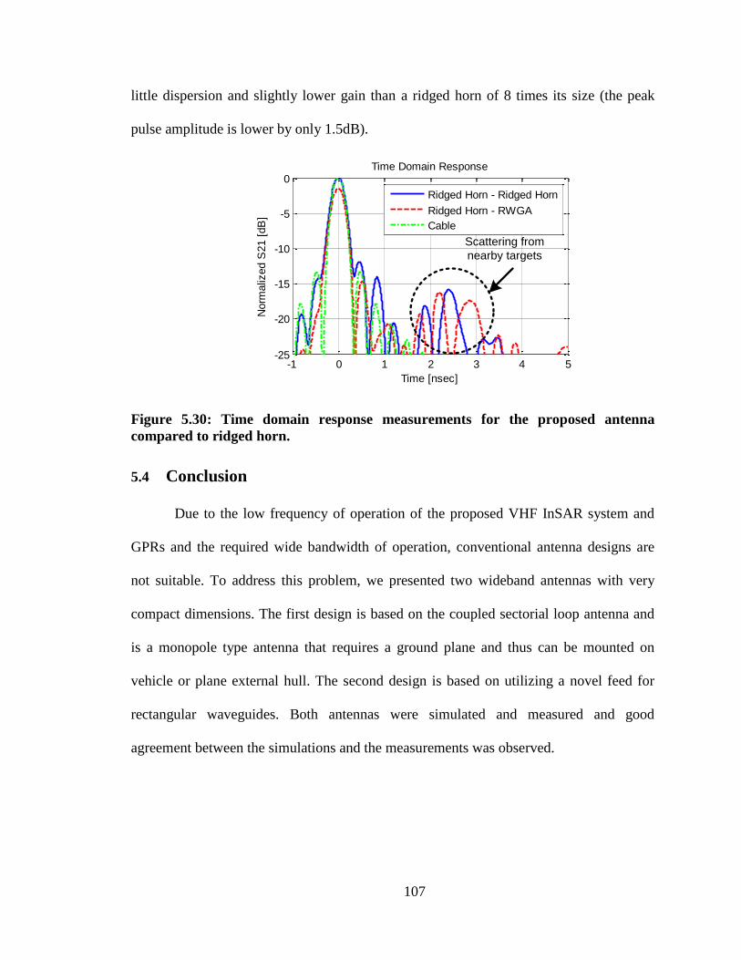
107

little dispersion and slightly lower gain than a ridged horn of 8 times its size (the peak

pulse amplitude is lower by only 1.5dB).

-1 0 1 2 3 4 5-25

-20

-15

-10

-5

0

Time [nsec]

Norm

aliz

ed S

21 [

dB

]

Time Domain Response

Ridged Horn - Ridged Horn

Ridged Horn - RWGA

Cable

Scattering from

nearby targets

Figure 5.30: Time domain response measurements for the proposed antenna

compared to ridged horn.

5.4 Conclusion

Due to the low frequency of operation of the proposed VHF InSAR system and

GPRs and the required wide bandwidth of operation, conventional antenna designs are

not suitable. To address this problem, we presented two wideband antennas with very

compact dimensions. The first design is based on the coupled sectorial loop antenna and

is a monopole type antenna that requires a ground plane and thus can be mounted on

vehicle or plane external hull. The second design is based on utilizing a novel feed for

rectangular waveguides. Both antennas were simulated and measured and good

agreement between the simulations and the measurements was observed.

108

Chapter 6

High Isolation T/R UWB Antenna Pair

In airborne radars scenarios, there is a large time difference (compared to the

transmitted pulse width) between the transmitted pulse and the backscattered signal from

the target. This large time difference allows the use of time domain switching between

the transmitter and receiver to separate the transmitted signal and the received signal.

This prevents saturating the receiver due to the large magnitude difference between the

transmitted and received signals. However, in GPR and other short distance radars, this

time difference is not as large. In such case, the isolation between the transmitted and

received signals is achieved by using two antennas and maximizing the isolation between

them. In this chapter, we discuss the importance of this isolation in Radar and in

communication systems. We then present typical examples of such antenna pairs. It is

shown that these pairs have to be separated relatively far from each other to get better

isolation. To address this problem, we present the development of a new cavity backed

CSLA antenna pair that can provide good isolation in a relatively compact size.

6.1 Introduction and Motivation

Ultra-wideband antennas are considered critical components of ultra-wideband

radar and communication systems that affect the performance and complexity of such

systems. In radar applications, antennas are desired to have good front-to-back ratio,

stable radiation characteristics, and be non-dispersive with well-defined and stable

radiation phase center. Many radar systems that require high sensitivity use two separate

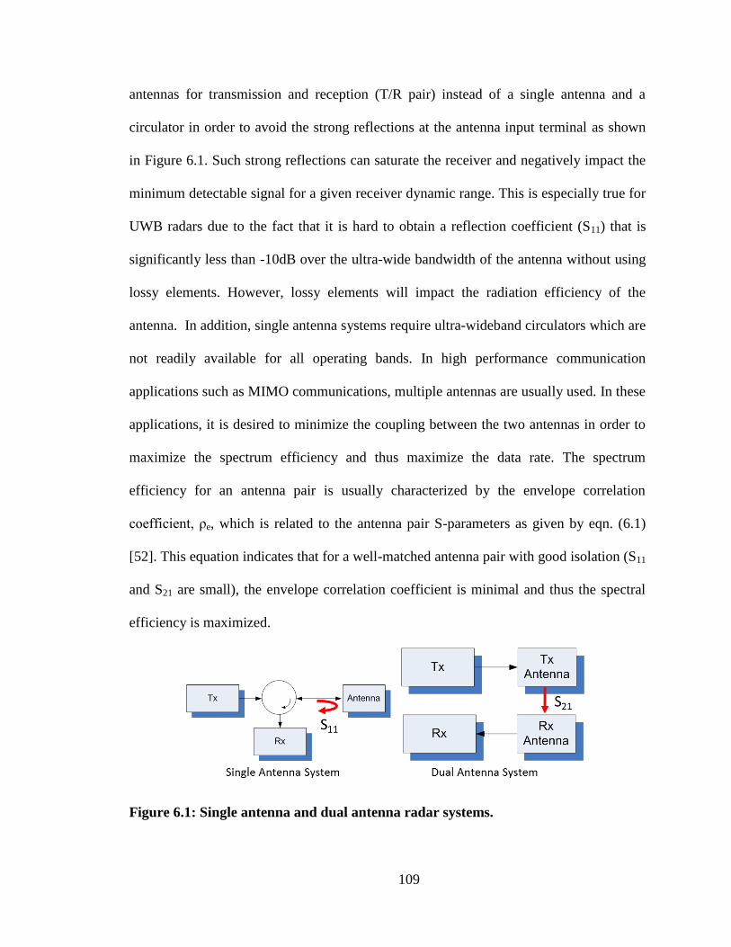
109

antennas for transmission and reception (T/R pair) instead of a single antenna and a

circulator in order to avoid the strong reflections at the antenna input terminal as shown

in Figure 6.1. Such strong reflections can saturate the receiver and negatively impact the

minimum detectable signal for a given receiver dynamic range. This is especially true for

UWB radars due to the fact that it is hard to obtain a reflection coefficient (S11) that is

significantly less than -10dB over the ultra-wide bandwidth of the antenna without using

lossy elements. However, lossy elements will impact the radiation efficiency of the

antenna. In addition, single antenna systems require ultra-wideband circulators which are

not readily available for all operating bands. In high performance communication

applications such as MIMO communications, multiple antennas are usually used. In these

applications, it is desired to minimize the coupling between the two antennas in order to

maximize the spectrum efficiency and thus maximize the data rate. The spectrum

efficiency for an antenna pair is usually characterized by the envelope correlation

coefficient, ρe, which is related to the antenna pair S-parameters as given by eqn. (6.1)

[52]. This equation indicates that for a well-matched antenna pair with good isolation (S11

and S21 are small), the envelope correlation coefficient is minimal and thus the spectral

efficiency is maximized.

Figure 6.1: Single antenna and dual antenna radar systems.

110

( )( ) (6.1)

Single directional UWB antenna designs are presented in many publications and

some of the designs were presented in the previous chapter. Some the standard techniques

for increasing the isolation between two such antennas are shown in Figure 6.2 (a) – (c)

and can be summarized as follows:

1. Increasing the physical separation between the two antennas. This is

based on that the main coupling component is the near field coupling

which decreases very rapidly with distance. This has the advantage that

the isolation is high over a very wideband and further increases with

the frequency. However, the overall system size increases. Also, larger

separations violate the requirement that the two antennas should have

very close phase centers so that the assumptions used in the single

antenna system are still valid in the two antenna system (in order not to

increase the complexity of the processing).

2. Adding lossy absorbing foam between the elements [53]. The main

purpose of the absorbing foam is to absorb the coupled signal between

the two antennas. This again results in good wide band isolation.

However, this absorbing foam, since it is in the near field of the

antenna, usually has the undesired characteristic of absorbing the

transmitted signal from the antenna leading to significant decrease in

the antenna radiation efficiency. As discussed in the previous chapter,

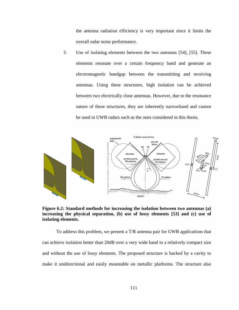
111

the antenna radiation efficiency is very important since it limits the

overall radar noise performance.

3. Use of isolating elements between the two antennas [54], [55]. These

elements resonate over a certain frequency band and generate an

electromagnetic bandgap between the transmitting and receiving

antennas. Using these structures, high isolation can be achieved

between two electrically close antennas. However, due to the resonance

nature of these structures, they are inherently narrowband and cannot

be used in UWB radars such as the ones considered in this thesis.

Figure 6.2: Standard methods for increasing the isolation between two antennas (a)

increasing the physical separation, (b) use of lossy elements [53] and (c) use of

isolating elements.

To address this problem, we present a T/R antenna pair for UWB applications that

can achieve isolation better than 20dB over a very wide band in a relatively compact size

and without the use of lossy elements. The proposed structure is backed by a cavity to

make it unidirectional and easily mountable on metallic platforms. The structure also

112

allows placement of electronics directly behind the antenna which can further reduce the

overall system size.

6.2 Antenna Structure and Operation

The proposed antenna structure is shown in Figure 6.3 (a) and (b). It consists of

two coupled sectorial loops antennas (CSLA) separated by a ground plane and fed using a

tapered microstrip line. The final antenna structure is achieved through the following

steps:

1- We started with the original balanced CSLA placed in front of a cylindrical cavity.

The cavity creates two significant problems for the antenna. The first problem is

that the minimum operating frequency of the original CSLA is increased

significantly due to the existence of the back metal plate. The second problem

pertains to the generation of in-band cavity resonances which can severely limit the

contiguous bandwidth of operation as shown in Figure 6.4 (b) and (c).

2- In order to retrieve the lost bandwidth (push the minimum operating frequency

lower), we placed the two annular slots of width dslot between the CSLA edge and

the rim of the cavity as shown in Figure 6.5 (a) and (c).

3- In order to suppress the in-band resonances we placed wedge shaped metallic fins

inside the cavity. The shape of this fin has to be optimized as a tradeoff between

suppressing the internal cavity modes and the bandwidth. This is shown in Figure

6.5 (b) and (c).

4- Finally to convert the single antenna into a T/R pair we split the antenna at its

electrical symmetry plane and used two individual unbalanced feeds instead of the

original balanced feed. Each feed consists of a linearly tapered microstrip line

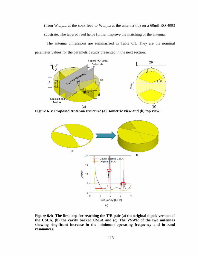
113

(from Wms_start at the coax feed to Wms_end at the antenna tip) on a 60mil RO 4003

substrate. The tapered feed helps further improve the matching of the antenna.

The antenna dimensions are summarized in Table 6.1. They are the nominal

parameter values for the parametric study presented in the next section.

Rogers RO4003C Substrate

Coaxial Feed Position

Tapered Microstr

ip

Line

hcyl

hse

p

Fin

hfinh

fin

2

X

YZ

wse

p

2R

dslo

t

α

(a) (b)

Figure 6.3: Proposed Antenna structure (a) isometric view and (b) top view.

(a)

(b)

(c)

Figure 6.4: The first step for reaching the T/R pair (a) the original dipole version of

the CSLA, (b) the cavity backed CSLA and (c) The VSWR of the two antennas

showing singificant increase in the minimum operating frequency and in-band

resonances.

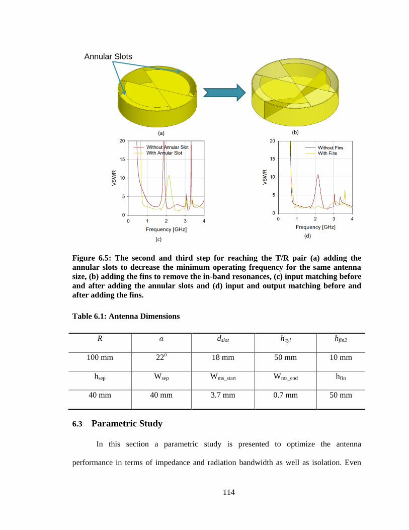
114

Annular Slots

(a)

(c)

(b)

(d)

Figure 6.5: The second and third step for reaching the T/R pair (a) adding the

annular slots to decrease the minimum operating frequency for the same antenna

size, (b) adding the fins to remove the in-band resonances, (c) input matching before

and after adding the annular slots and (d) input and output matching before and

after adding the fins.

Table 6.1: Antenna Dimensions

R α dslot hcyl hfin2

100 mm 22o 18 mm 50 mm 10 mm

hsep Wsep Wms_start Wms_end hfin

40 mm 40 mm 3.7 mm 0.7 mm 50 mm

6.3 Parametric Study

In this section a parametric study is presented to optimize the antenna

performance in terms of impedance and radiation bandwidth as well as isolation. Even

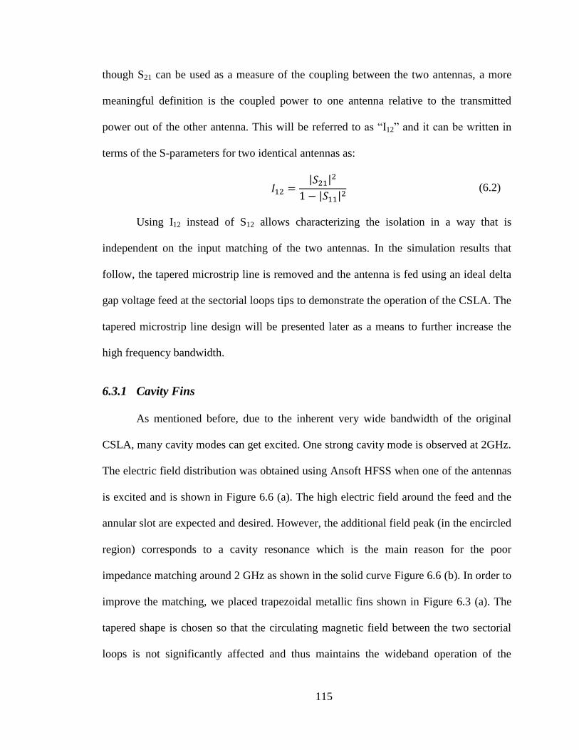
115

though S21 can be used as a measure of the coupling between the two antennas, a more

meaningful definition is the coupled power to one antenna relative to the transmitted

power out of the other antenna. This will be referred to as ―I12‖ and it can be written in

terms of the S-parameters for two identical antennas as:

(6.2)

Using I12 instead of S12 allows characterizing the isolation in a way that is

independent on the input matching of the two antennas. In the simulation results that

follow, the tapered microstrip line is removed and the antenna is fed using an ideal delta

gap voltage feed at the sectorial loops tips to demonstrate the operation of the CSLA. The

tapered microstrip line design will be presented later as a means to further increase the

high frequency bandwidth.

6.3.1 Cavity Fins

As mentioned before, due to the inherent very wide bandwidth of the original

CSLA, many cavity modes can get excited. One strong cavity mode is observed at 2GHz.

The electric field distribution was obtained using Ansoft HFSS when one of the antennas

is excited and is shown in Figure 6.6 (a). The high electric field around the feed and the

annular slot are expected and desired. However, the additional field peak (in the encircled

region) corresponds to a cavity resonance which is the main reason for the poor

impedance matching around 2 GHz as shown in the solid curve Figure 6.6 (b). In order to

improve the matching, we placed trapezoidal metallic fins shown in Figure 6.3 (a). The

tapered shape is chosen so that the circulating magnetic field between the two sectorial

loops is not significantly affected and thus maintains the wideband operation of the

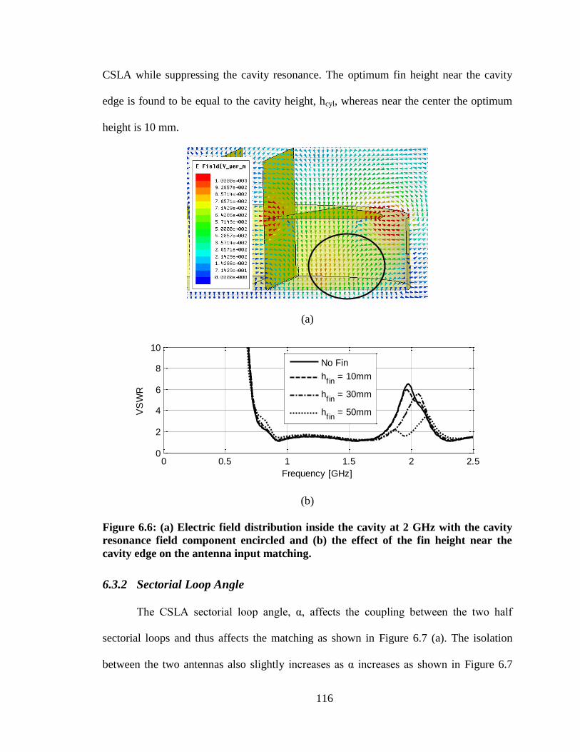
116

CSLA while suppressing the cavity resonance. The optimum fin height near the cavity

edge is found to be equal to the cavity height, hcyl, whereas near the center the optimum

height is 10 mm.

(a)

(b)

Figure 6.6: (a) Electric field distribution inside the cavity at 2 GHz with the cavity

resonance field component encircled and (b) the effect of the fin height near the

cavity edge on the antenna input matching.

6.3.2 Sectorial Loop Angle

The CSLA sectorial loop angle, α, affects the coupling between the two half

sectorial loops and thus affects the matching as shown in Figure 6.7 (a). The isolation

between the two antennas also slightly increases as α increases as shown in Figure 6.7

0 0.5 1 1.5 2 2.50

2

4

6

8

10

Frequency [GHz]

VS

WR

No Fin

hf in

= 10mm

hf in

= 30mm

hf in

= 50mm

117

(b). This is probably due to the movement of the radiation centers towards the annular

slots and away from the center thus increasing the effective distance between the two

antennas. To obtain the best matching over the widest bandwidth, we chose α equal to

22o.


function of the sectorial loop angle, α.

6.3.3 The Cavity Height

The second parameter to consider is the cavity height, hcyl. Its effect on the

matching and isolation is shown in Figure 6.8 (a) and (b), respectively. Increasing the

cavity height, hcyl, improves the matching at lower frequencies since it reduces the effect

of the bottom cavity wall on the coupling between the two antennas. However, deep

cavities have more resonances within the frequency band of interest which limits the

overall bandwidth of the antenna as shown in the figure. Also, increasing the cavity

0 0.5 1 1.5 2 2.50

1

2

3

4

5

Frequency [GHz]

(a)

VS

WR

0 0.5 1 1.5 2 2.5-40

-30

-20

-10

Frequency [GHz]

(b)

I 12 [

dB

]

= 10o

= 20o

= 30o

= 40o

= 10o

= 20o

= 30o

= 40o

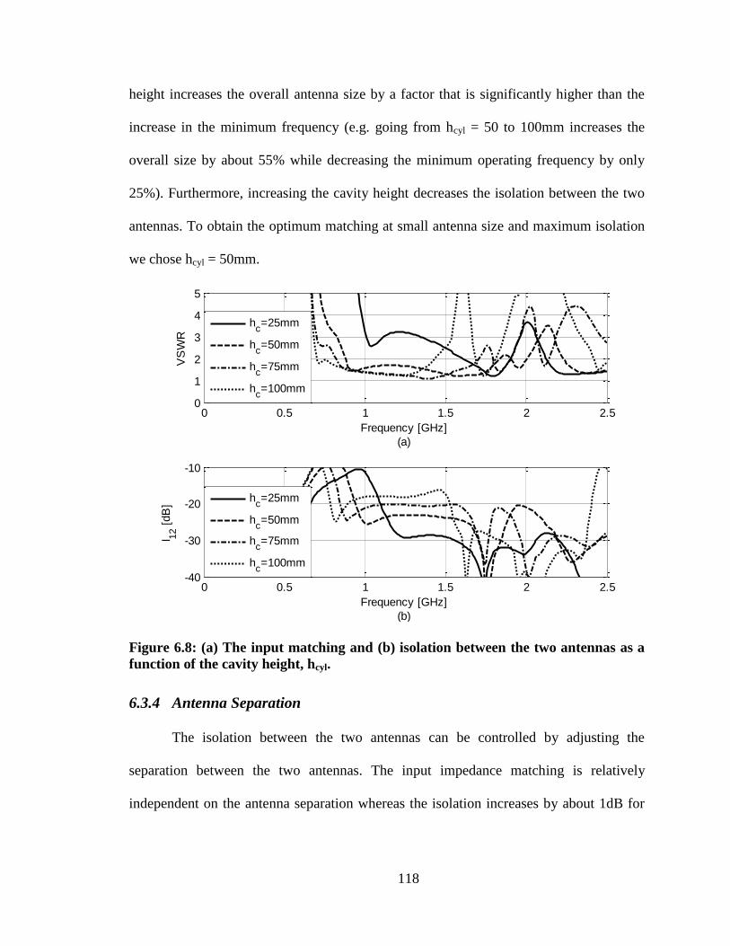
118

height increases the overall antenna size by a factor that is significantly higher than the

increase in the minimum frequency (e.g. going from hcyl = 50 to 100mm increases the

overall size by about 55% while decreasing the minimum operating frequency by only

25%). Furthermore, increasing the cavity height decreases the isolation between the two

antennas. To obtain the optimum matching at small antenna size and maximum isolation

we chose hcyl = 50mm.


function of the cavity height, hcyl.

6.3.4 Antenna Separation

The isolation between the two antennas can be controlled by adjusting the

separation between the two antennas. The input impedance matching is relatively

independent on the antenna separation whereas the isolation increases by about 1dB for

0 0.5 1 1.5 2 2.50

1

2

3

4

5

Frequency [GHz]

(a)

VS

WR

0 0.5 1 1.5 2 2.5-40

-30

-20

-10

Frequency [GHz]

(b)

I 12 [

dB

]

hc=25mm

hc=50mm

hc=75mm

hc=100mm

hc=25mm

hc=50mm

hc=75mm

hc=100mm

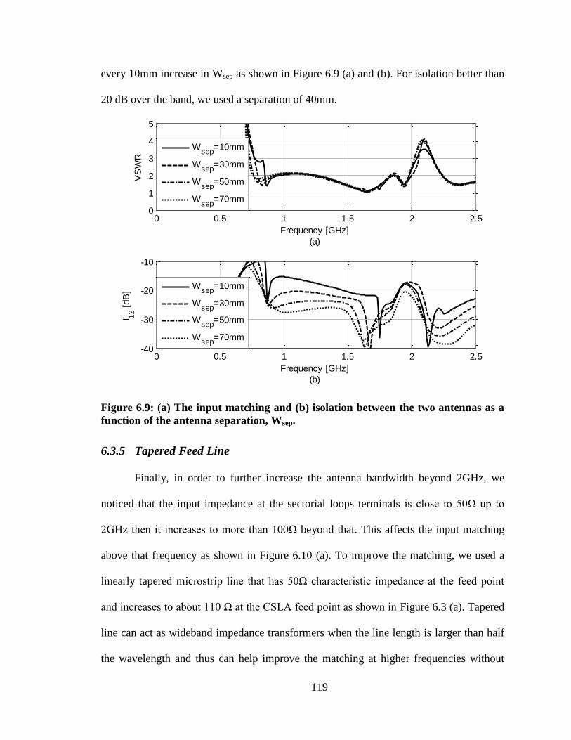
119

every 10mm increase in Wsep as shown in Figure 6.9 (a) and (b). For isolation better than

20 dB over the band, we used a separation of 40mm.


function of the antenna separation, Wsep.

6.3.5 Tapered Feed Line

Finally, in order to further increase the antenna bandwidth beyond 2GHz, we

noticed that the input impedance at the sectorial loops terminals is close to 50Ω up to

2GHz then it increases to more than 100Ω beyond that. This affects the input matching

above that frequency as shown in Figure 6.10 (a). To improve the matching, we used a

linearly tapered microstrip line that has 50Ω characteristic impedance at the feed point

and increases to about 110 Ω at the CSLA feed point as shown in Figure 6.3 (a). Tapered

line can act as wideband impedance transformers when the line length is larger than half

the wavelength and thus can help improve the matching at higher frequencies without

0 0.5 1 1.5 2 2.50

1

2

3

4

5

Frequency [GHz]

(a)

VS

WR

0 0.5 1 1.5 2 2.5-40

-30

-20

-10

Frequency [GHz]

(b)

I 12 [

dB

]

Wsep

=10mm

Wsep

=30mm

Wsep

=50mm

Wsep

=70mm

Wsep

=10mm

Wsep

=30mm

Wsep

=50mm

Wsep

=70mm

120

severely affecting the matching at the lower frequencies. The design is shown in Figure

6.10 (b) where it can be seen that decreasing the taper width helps improve the matching

beyond 2GHz. Choosing an end taper width, Wend, of 0.7mm gives good matching at both

the high and low frequency portions of the band as shown in the figure.

Figure 6.10: (a) The input impedance at one antenna port when the other port is

matched and (b) the input VSWR as a function of the tapered microstrip line end

width.

0 0.5 1 1.5 2 2.5-200

-100

0

100

200

Frequency [GHz]

(a)

Zin

[

]

0 0.5 1 1.5 2 2.50

1

2

3

4

5

Frequency [GHz]

(b)

VS

WR

Re

Im

Wend

=0.3mm

Wend

=0.7mm

Wend

=1.5mm

Wend

=2.7mm

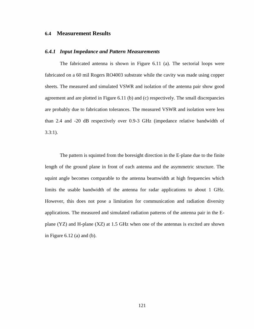
121

6.4 Measurement Results

6.4.1 Input Impedance and Pattern Measurements

The fabricated antenna is shown in Figure 6.11 (a). The sectorial loops were

fabricated on a 60 mil Rogers RO4003 substrate while the cavity was made using copper

sheets. The measured and simulated VSWR and isolation of the antenna pair show good

agreement and are plotted in Figure 6.11 (b) and (c) respectively. The small discrepancies

are probably due to fabrication tolerances. The measured VSWR and isolation were less

than 2.4 and -20 dB respectively over 0.9-3 GHz (impedance relative bandwidth of

3.3:1).

The pattern is squinted from the boresight direction in the E-plane due to the finite

length of the ground plane in front of each antenna and the asymmetric structure. The

squint angle becomes comparable to the antenna beamwidth at high frequencies which

limits the usable bandwidth of the antenna for radar applications to about 1 GHz.

However, this does not pose a limitation for communication and radiation diversity

applications. The measured and simulated radiation patterns of the antenna pair in the E-

plane (YZ) and H-plane (XZ) at 1.5 GHz when one of the antennas is excited are shown

in Figure 6.12 (a) and (b).

122

(a)

Figure 6.11: (a) The fabricated antenna pair and the measured and simulated (b)

input VSWR and (c) isolation.

0 0.5 1 1.5 2 2.5 30

1

2

3

4

5

Frequency [GHz]

(b)

Input

VS

WR

0 0.5 1 1.5 2 2.5 3-40

-30

-20

-10

0

Frequency [GHz]

(c)

I 12[d

B]

Measurement

Simulation

Measurement

Simulation

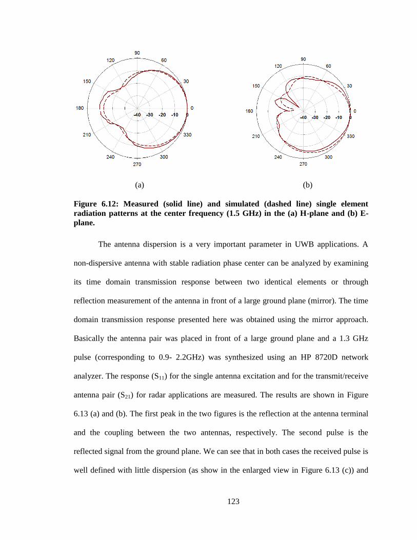
123

(a) (b)

Figure 6.12: Measured (solid line) and simulated (dashed line) single element

radiation patterns at the center frequency (1.5 GHz) in the (a) H-plane and (b) E-

plane.

The antenna dispersion is a very important parameter in UWB applications. A

non-dispersive antenna with stable radiation phase center can be analyzed by examining

its time domain transmission response between two identical elements or through

reflection measurement of the antenna in front of a large ground plane (mirror). The time

domain transmission response presented here was obtained using the mirror approach.

Basically the antenna pair was placed in front of a large ground plane and a 1.3 GHz

pulse (corresponding to 0.9- 2.2GHz) was synthesized using an HP 8720D network

analyzer. The response (S11) for the single antenna excitation and for the transmit/receive

antenna pair (S21) for radar applications are measured. The results are shown in Figure

6.13 (a) and (b). The first peak in the two figures is the reflection at the antenna terminal

and the coupling between the two antennas, respectively. The second pulse is the

reflected signal from the ground plane. We can see that in both cases the received pulse is

well defined with little dispersion (as show in the enlarged view in Figure 6.13 (c)) and

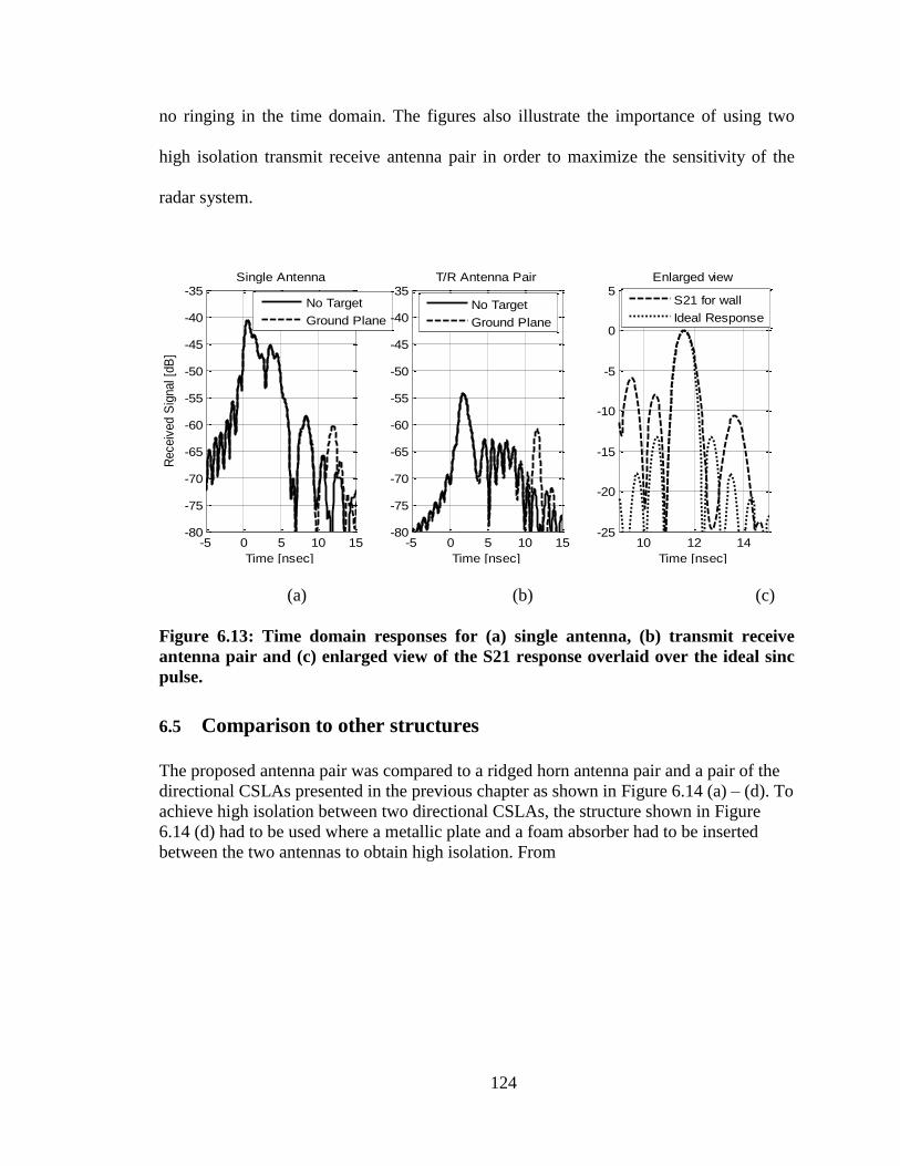
124

no ringing in the time domain. The figures also illustrate the importance of using two

high isolation transmit receive antenna pair in order to maximize the sensitivity of the

radar system.

(a) (b) (c)

Figure 6.13: Time domain responses for (a) single antenna, (b) transmit receive

antenna pair and (c) enlarged view of the S21 response overlaid over the ideal sinc

pulse.

6.5 Comparison to other structures

The proposed antenna pair was compared to a ridged horn antenna pair and a pair of the

directional CSLAs presented in the previous chapter as shown in Figure 6.14 (a) – (d). To

achieve high isolation between two directional CSLAs, the structure shown in Figure

6.14 (d) had to be used where a metallic plate and a foam absorber had to be inserted

between the two antennas to obtain high isolation. From

-5 0 5 10 15-80

-75

-70

-65

-60

-55

-50

-45

-40

-35

Time [nsec]

Receiv

ed S

ignal [d

B]

Single Antenna

No Target

Ground Plane

-5 0 5 10 15-80

-75

-70

-65

-60

-55

-50

-45

-40

-35

Time [nsec]

T/R Antenna Pair

No Target

Ground Plane

10 12 14-25

-20

-15

-10

-5

0

5

Time [nsec]

Enlarged view

S21 for wall

Ideal Response

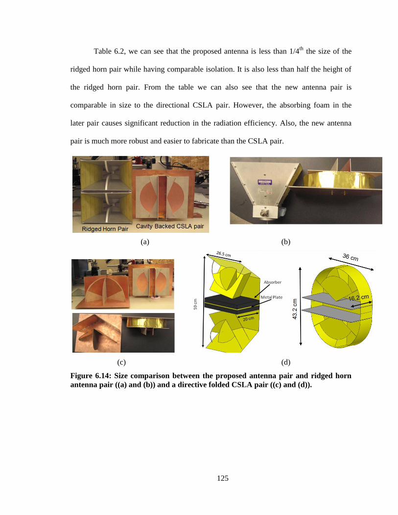
125

Table 6.2, we can see that the proposed antenna is less than 1/4th

the size of the

ridged horn pair while having comparable isolation. It is also less than half the height of

the ridged horn pair. From the table we can also see that the new antenna pair is

comparable in size to the directional CSLA pair. However, the absorbing foam in the

later pair causes significant reduction in the radiation efficiency. Also, the new antenna

pair is much more robust and easier to fabricate than the CSLA pair.

(a) (b)

(c) (d)

Figure 6.14: Size comparison between the proposed antenna pair and ridged horn

antenna pair ((a) and (b)) and a directive folded CSLA pair ((c) and (d)).

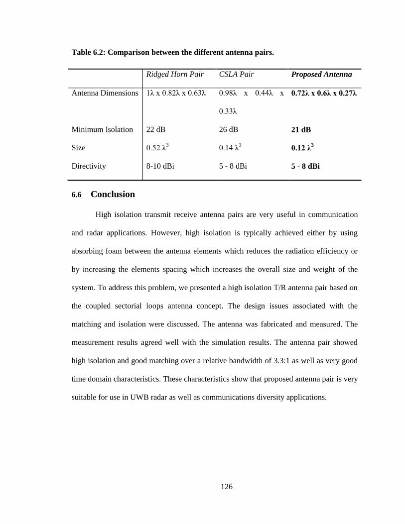
126

Table 6.2: Comparison between the different antenna pairs.

Ridged Horn Pair CSLA Pair Proposed Antenna

Antenna Dimensions 1λ x 0.82λ x 0.63λ 0.98λ x 0.44λ x

0.33λ

0.72λ x 0.6λ x 0.27λ

Minimum Isolation 22 dB 26 dB 21 dB

Size 0.52 λ3 0.14 λ

3 0.12 λ

3

Directivity 8-10 dBi 5 - 8 dBi 5 - 8 dBi

6.6 Conclusion

High isolation transmit receive antenna pairs are very useful in communication

and radar applications. However, high isolation is typically achieved either by using

absorbing foam between the antenna elements which reduces the radiation efficiency or

by increasing the elements spacing which increases the overall size and weight of the

system. To address this problem, we presented a high isolation T/R antenna pair based on

the coupled sectorial loops antenna concept. The design issues associated with the

matching and isolation were discussed. The antenna was fabricated and measured. The

measurement results agreed well with the simulation results. The antenna pair showed

high isolation and good matching over a relative bandwidth of 3.3:1 as well as very good

time domain characteristics. These characteristics show that proposed antenna pair is very

suitable for use in UWB radar as well as communications diversity applications.

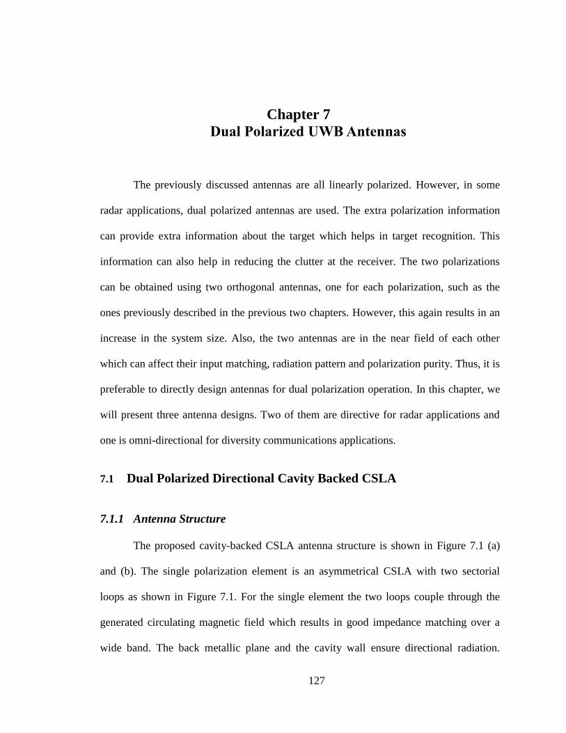
127

Chapter 7

Dual Polarized UWB Antennas

The previously discussed antennas are all linearly polarized. However, in some

radar applications, dual polarized antennas are used. The extra polarization information

can provide extra information about the target which helps in target recognition. This

information can also help in reducing the clutter at the receiver. The two polarizations

can be obtained using two orthogonal antennas, one for each polarization, such as the

ones previously described in the previous two chapters. However, this again results in an

increase in the system size. Also, the two antennas are in the near field of each other

which can affect their input matching, radiation pattern and polarization purity. Thus, it is

preferable to directly design antennas for dual polarization operation. In this chapter, we

will present three antenna designs. Two of them are directive for radar applications and

one is omni-directional for diversity communications applications.

7.1 Dual Polarized Directional Cavity Backed CSLA

7.1.1 Antenna Structure

The proposed cavity-backed CSLA antenna structure is shown in Figure 7.1 (a)

and (b). The single polarization element is an asymmetrical CSLA with two sectorial

loops as shown in Figure 7.1. For the single element the two loops couple through the

generated circulating magnetic field which results in good impedance matching over a

wide band. The back metallic plane and the cavity wall ensure directional radiation.

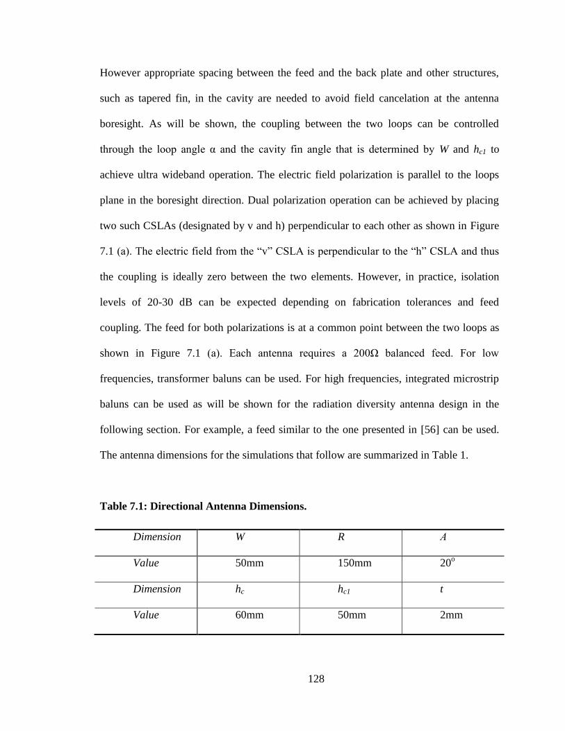
128

However appropriate spacing between the feed and the back plate and other structures,

such as tapered fin, in the cavity are needed to avoid field cancelation at the antenna

boresight. As will be shown, the coupling between the two loops can be controlled

through the loop angle α and the cavity fin angle that is determined by W and hc1 to

achieve ultra wideband operation. The electric field polarization is parallel to the loops

plane in the boresight direction. Dual polarization operation can be achieved by placing

two such CSLAs (designated by v and h) perpendicular to each other as shown in Figure

7.1 (a). The electric field from the ―v‖ CSLA is perpendicular to the ―h‖ CSLA and thus

the coupling is ideally zero between the two elements. However, in practice, isolation

levels of 20-30 dB can be expected depending on fabrication tolerances and feed

coupling. The feed for both polarizations is at a common point between the two loops as

shown in Figure 7.1 (a). Each antenna requires a 200Ω balanced feed. For low

frequencies, transformer baluns can be used. For high frequencies, integrated microstrip

baluns can be used as will be shown for the radiation diversity antenna design in the

following section. For example, a feed similar to the one presented in [56] can be used.

The antenna dimensions for the simulations that follow are summarized in Table 1.

Table 7.1: Directional Antenna Dimensions.

Dimension W R Α

Value 50mm 150mm 20o

Dimension hc hc1 t

Value 60mm 50mm 2mm

129

R

Ev

Eh“h” CSLA

“v” CSLA

Cavity

R

α W

hc1

hc

t

Feed

v

h

(a) (b)

Figure 7.1: (a) Dual-polarized cavity-backed CSLA structure (cavity walls

transparent for clarity) and (b) side view along one of the polarization planes. (The

antenna is not drawn with the correct dimensions to clarify some of the dimensions.)

7.1.2 Parametric Study

The sectorial loop angle, α, affects the matching as shown in Figure 7.2 (a) since

it controls the coupling between the two loops. It has a small effect on the directivity as

shown in Figure 7.2 (b). We chose α = 20o since it gives good impedance matching over

the desired band and has the lowest minimum operating frequency thus resulting in the

smallest antenna size.

Increasing the back loop height, hc1, improves the impedance matching as shown

in Figure 7.3 (a) since it reduces the impact of the metallic plane on the magnetic

coupling between the two loops. However, large values results in cavity resonances in the

band (e.g. at hc1 = 11cm). Furthermore, larger cavity heights result in lower directivity at

higher frequencies as shown in Figure 7.3 (b). This is due to the destructive interference

130

between the direct ray from the loop and the reflected ray from the metallic plate at the

back of the cavity. To achieve good matching while maintaining wide gain bandwidth,

we chose hc1 = 50 mm.

A unique feature in this antenna is that its directivity can be easily controlled by

adjusting the cavity sidewall height hc, increasing hc reduces the beamwidth and thus

increases the directivity since it decreases the radiation along angles away from the

boresight as shown in Figure 7.4 (a). However, since increasing hc reduces the radiation

in other directions and affects the coupling between the two loops, it increases the

minimum operating frequency of the antenna as shown in Figure 7.4 (b). This is expected

due to the fundamental relation between the antenna gain and its size which predicts

higher gain for antennas with larger electrical dimensions.

131

(a)

(b)

Figure 7.2: Effect of the sectorial loop angle, α, on (a) the input matching and (b) the

H-plane radiation pattern at 1.75 GHz.

0.5 1 1.5 20

1

2

3

4

5

Frequency [GHz]

VS

WR

= 10o

= 20o

= 30o

= 40o

Frequency [GHz]

VS

WR

H-Plane [1.75GHz]

-20-100

0

45

90

135

180

225

270

315

= 10o

= 20o

= 30o

= 40o

132

(a)

(b)

Figure 7.3: Effect of the cavity height, hc1, on the antenna (a) input matching and (b)

E-plane radiation pattern at 1.7 GHz.

0.5 1 1.5 20

1

2

3

4

5

Frequency [GHz]

VS

WR

hc1

= 20 mm

hc1

= 50 mm

hc1

= 80 mm

hc1

= 110 mm

Frequency [GHz]

E-Plane [1.75GHz]

-20-100

0

45

90

135

180

225

270

315

hc1

= 20 mm

hc1

= 50 mm

hc1

= 80 mm

hc1

= 110 mm

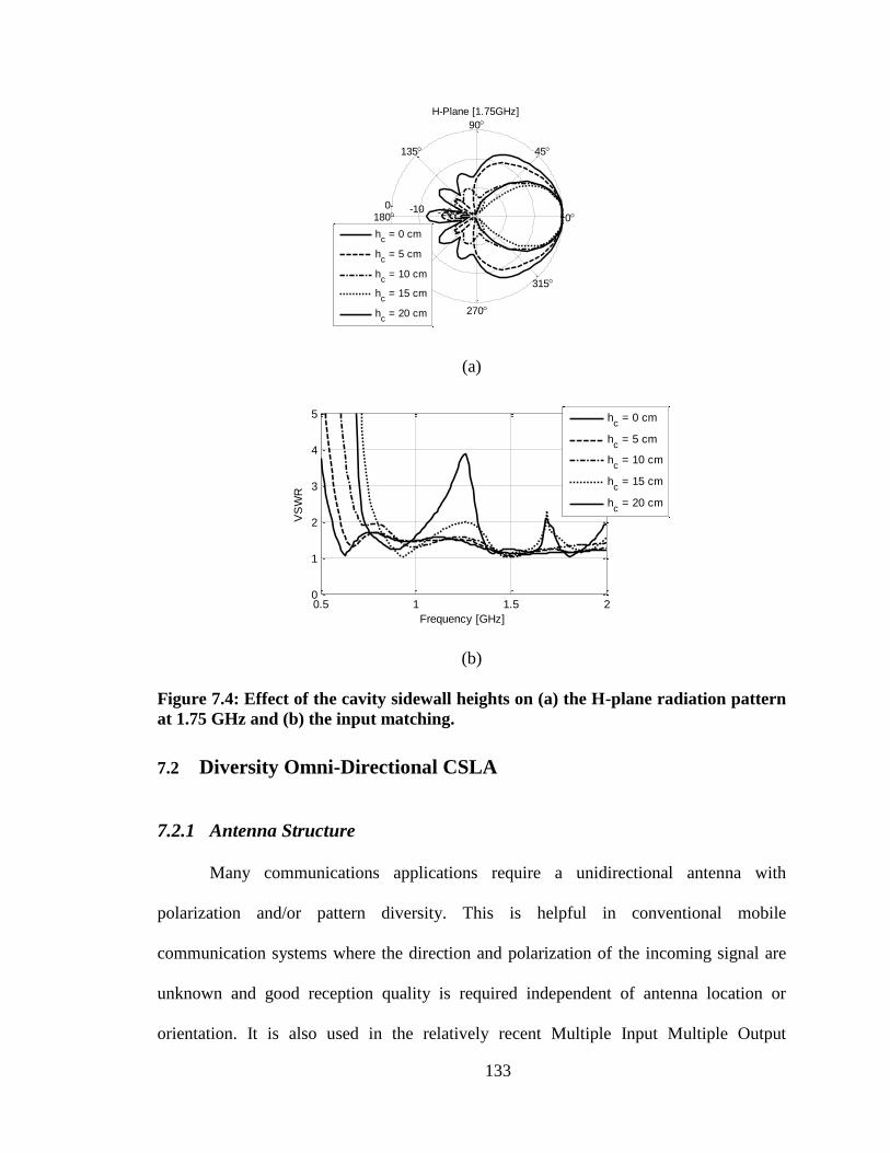
133

(a)

(b)

Figure 7.4: Effect of the cavity sidewall heights on (a) the H-plane radiation pattern

at 1.75 GHz and (b) the input matching.

7.2 Diversity Omni-Directional CSLA

7.2.1 Antenna Structure

Many communications applications require a unidirectional antenna with

polarization and/or pattern diversity. This is helpful in conventional mobile

communication systems where the direction and polarization of the incoming signal are

unknown and good reception quality is required independent of antenna location or

orientation. It is also used in the relatively recent Multiple Input Multiple Output

H-Plane [1.75GHz]

-20-100

0

45

90

135

180

225

270

315

hc = 0 cm

hc = 5 cm

hc = 10 cm

hc = 15 cm

hc = 20 cm

0.5 1 1.5 20

1

2

3

4

5

Frequency [GHz]

VS

WR

hc = 0 cm

hc = 5 cm

hc = 10 cm

hc = 15 cm

hc = 20 cm

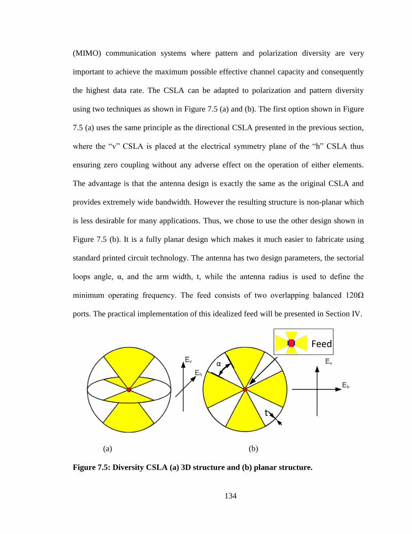
134

(MIMO) communication systems where pattern and polarization diversity are very

important to achieve the maximum possible effective channel capacity and consequently

the highest data rate. The CSLA can be adapted to polarization and pattern diversity

using two techniques as shown in Figure 7.5 (a) and (b). The first option shown in Figure

7.5 (a) uses the same principle as the directional CSLA presented in the previous section,

where the ―v‖ CSLA is placed at the electrical symmetry plane of the ―h‖ CSLA thus

ensuring zero coupling without any adverse effect on the operation of either elements.

The advantage is that the antenna design is exactly the same as the original CSLA and

provides extremely wide bandwidth. However the resulting structure is non-planar which

is less desirable for many applications. Thus, we chose to use the other design shown in

Figure 7.5 (b). It is a fully planar design which makes it much easier to fabricate using

standard printed circuit technology. The antenna has two design parameters, the sectorial

loops angle, α, and the arm width, t, while the antenna radius is used to define the

minimum operating frequency. The feed consists of two overlapping balanced 120Ω

ports. The practical implementation of this idealized feed will be presented in Section IV.

Feed

t

α

(a) (b)

Figure 7.5: Diversity CSLA (a) 3D structure and (b) planar structure.

135

The current distribution on the CSLA at 0.5 GHz for the horizontal polarization

feeding case is shown in Figure 7.6 (a) and (b) where we can see that the current is

circulating around the ―v‖ port resulting in no net current flowing into it and thus very

high isolation between the V and H polarization. This is expected since for balanced feed,

each port is at the virtual ground of the other port. It is also interesting to note the

direction of the current which shows two dual-sectorial-loops that are coupled together.

Those two dual-loops are common between the two feeding modes but the configuration

changes as shown in Figure 7.7 (a) and (b). This reuse of the loops is the reason that the

antenna dimensions are comparable to the original CSLA. The antenna could be matched

to 120Ω by controlling the sectorial loops angle as shown in Figure 7.8.

Ev

Eh

(a) (b)

Figure 7.6: Current distribution on the antenna for the two polarizations: (a)

horizontal and (b) vertical.

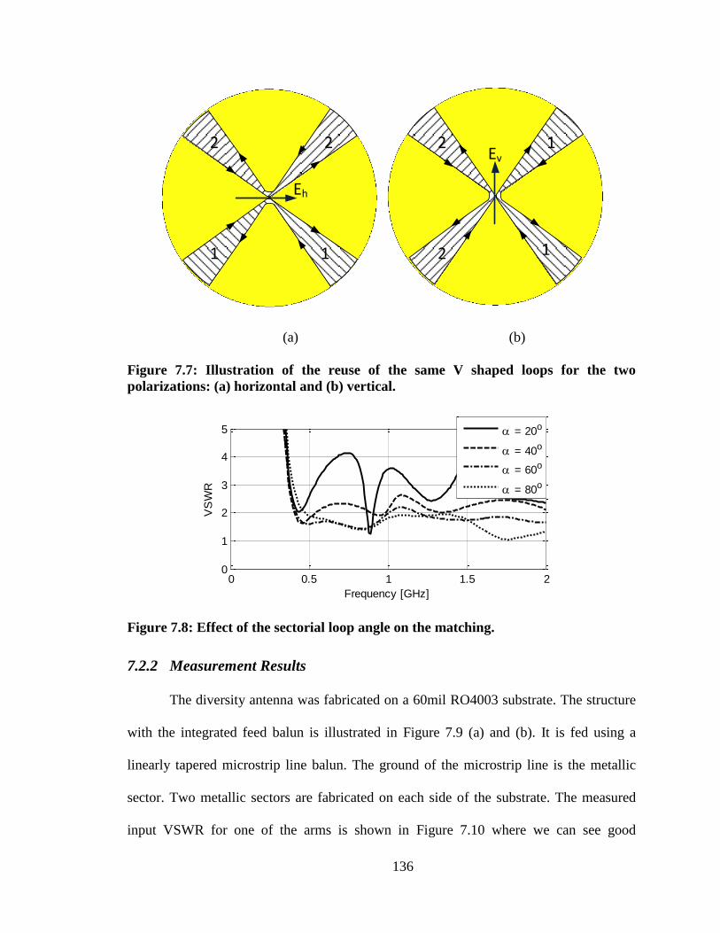
136

Ev

Eh

1

1

2

2

22

1 1

(a) (b)

Figure 7.7: Illustration of the reuse of the same V shaped loops for the two

polarizations: (a) horizontal and (b) vertical.

Figure 7.8: Effect of the sectorial loop angle on the matching.


The diversity antenna was fabricated on a 60mil RO4003 substrate. The structure

with the integrated feed balun is illustrated in Figure 7.9 (a) and (b). It is fed using a

linearly tapered microstrip line balun. The ground of the microstrip line is the metallic

sector. Two metallic sectors are fabricated on each side of the substrate. The measured

input VSWR for one of the arms is shown in Figure 7.10 where we can see good

0 0.5 1 1.5 20

1

2

3

4

5

Frequency [GHz]

VS

WR

= 20o

= 40o

= 60o

= 80o

137

agreement between the simulation and measurements. The antenna had an input VSWR

less than 2.5 over 0.48-2.4 GHz. The measured isolation between the two ports is

measured to be better than 25 dB as shown in Figure 7.10. The E- & H- plane radiation

patterns were also measured and are shown in Figure 7.11 together with the simulation

results and they both show very good agreement and a good omni-directional pattern over

more than one octave.

(a) (b)

Figure 7.9: (a) Structure of the fabricated diversity antenna and (b) enlarged view of

the feed region (darker yellow traces are on the bottom layer).

Frequency [GHz]0.5 1.0 1.5 2.0 2.5

VS

WR

0

2

4

6

8

10|S

21| [d

B]

-50

-45

-40

-35

-30

-25

-20

Measurement

Simulation

Figure 7.10: Input VSWR and isolation of the antenna.

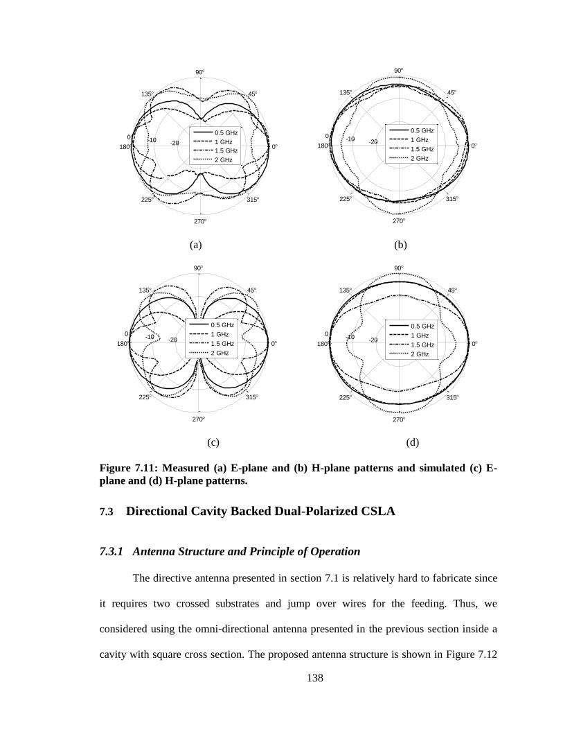
138

(a) (b)

(c) (d)

Figure 7.11: Measured (a) E-plane and (b) H-plane patterns and simulated (c) E-

plane and (d) H-plane patterns.

7.3 Directional Cavity Backed Dual-Polarized CSLA

7.3.1 Antenna Structure and Principle of Operation

The directive antenna presented in section 7.1 is relatively hard to fabricate since

it requires two crossed substrates and jump over wires for the feeding. Thus, we

considered using the omni-directional antenna presented in the previous section inside a

cavity with square cross section. The proposed antenna structure is shown in Figure 7.12

-20-100

0

45

90

135

180

225

270

315

0.5 GHz

1 GHz

1.5 GHz

2 GHz

-20-100

0

45

90

135

180

225

270

315

0.5 GHz

1 GHz

1.5 GHz

2 GHz

-20-100

0

45

90

135

180

225

270

315

0.5 GHz

1 GHz

1.5 GHz

2 GHz

-20-100

0

45

90

135

180

225

270

315

0.5 GHz

1 GHz

1.5 GHz

2 GHz

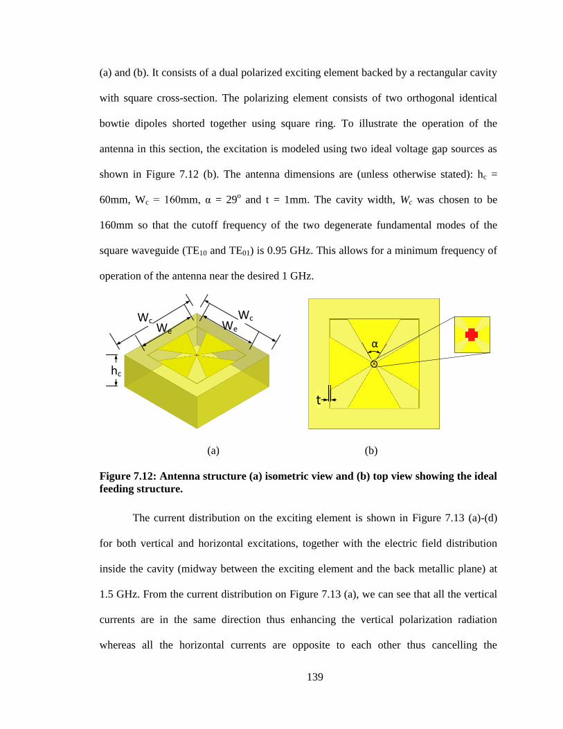
139

(a) and (b). It consists of a dual polarized exciting element backed by a rectangular cavity

with square cross-section. The polarizing element consists of two orthogonal identical

bowtie dipoles shorted together using square ring. To illustrate the operation of the

antenna in this section, the excitation is modeled using two ideal voltage gap sources as

shown in Figure 7.12 (b). The antenna dimensions are (unless otherwise stated): hc =

60mm, Wc = 160mm, α = 29o and t = 1mm. The cavity width, Wc was chosen to be

160mm so that the cutoff frequency of the two degenerate fundamental modes of the

square waveguide (TE10 and TE01) is 0.95 GHz. This allows for a minimum frequency of

operation of the antenna near the desired 1 GHz.

hc

WcWcWe We

t

α

(a) (b)

Figure 7.12: Antenna structure (a) isometric view and (b) top view showing the ideal

feeding structure.

The current distribution on the exciting element is shown in Figure 7.13 (a)-(d)

for both vertical and horizontal excitations, together with the electric field distribution

inside the cavity (midway between the exciting element and the back metallic plane) at

1.5 GHz. From the current distribution on Figure 7.13 (a), we can see that all the vertical

currents are in the same direction thus enhancing the vertical polarization radiation

whereas all the horizontal currents are opposite to each other thus cancelling the

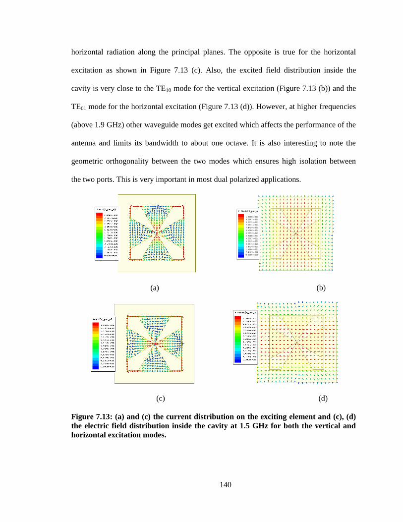
140

horizontal radiation along the principal planes. The opposite is true for the horizontal

excitation as shown in Figure 7.13 (c). Also, the excited field distribution inside the

cavity is very close to the TE10 mode for the vertical excitation (Figure 7.13 (b)) and the

TE01 mode for the horizontal excitation (Figure 7.13 (d)). However, at higher frequencies

(above 1.9 GHz) other waveguide modes get excited which affects the performance of the

antenna and limits its bandwidth to about one octave. It is also interesting to note the

geometric orthogonality between the two modes which ensures high isolation between

the two ports. This is very important in most dual polarized applications.

(a) (b)

(c) (d)

Figure 7.13: (a) and (c) the current distribution on the exciting element and (c), (d)

the electric field distribution inside the cavity at 1.5 GHz for both the vertical and

horizontal excitation modes.

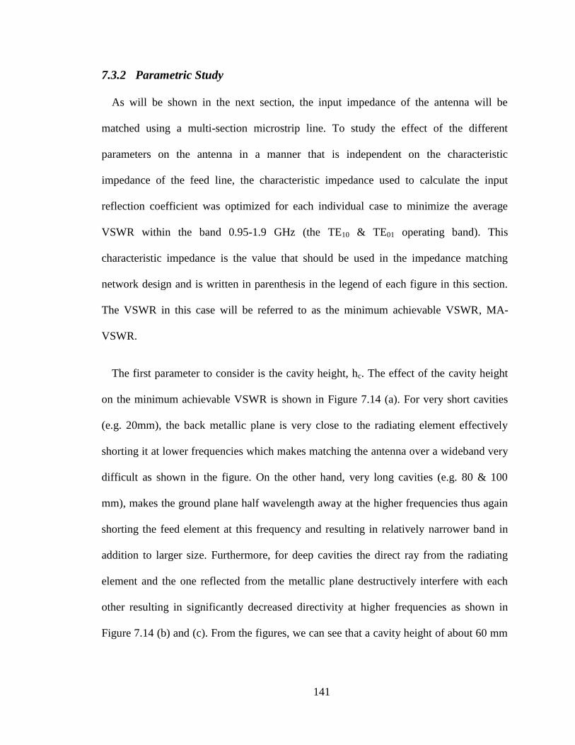
141


As will be shown in the next section, the input impedance of the antenna will be

matched using a multi-section microstrip line. To study the effect of the different

parameters on the antenna in a manner that is independent on the characteristic

impedance of the feed line, the characteristic impedance used to calculate the input

reflection coefficient was optimized for each individual case to minimize the average

VSWR within the band 0.95-1.9 GHz (the TE10 & TE01 operating band). This

characteristic impedance is the value that should be used in the impedance matching

network design and is written in parenthesis in the legend of each figure in this section.

The VSWR in this case will be referred to as the minimum achievable VSWR, MA-

VSWR.

The first parameter to consider is the cavity height, hc. The effect of the cavity height

on the minimum achievable VSWR is shown in Figure 7.14 (a). For very short cavities

(e.g. 20mm), the back metallic plane is very close to the radiating element effectively

shorting it at lower frequencies which makes matching the antenna over a wideband very

difficult as shown in the figure. On the other hand, very long cavities (e.g. 80 & 100

mm), makes the ground plane half wavelength away at the higher frequencies thus again

shorting the feed element at this frequency and resulting in relatively narrower band in

addition to larger size. Furthermore, for deep cavities the direct ray from the radiating

element and the one reflected from the metallic plane destructively interfere with each

other resulting in significantly decreased directivity at higher frequencies as shown in

Figure 7.14 (b) and (c). From the figures, we can see that a cavity height of about 60 mm

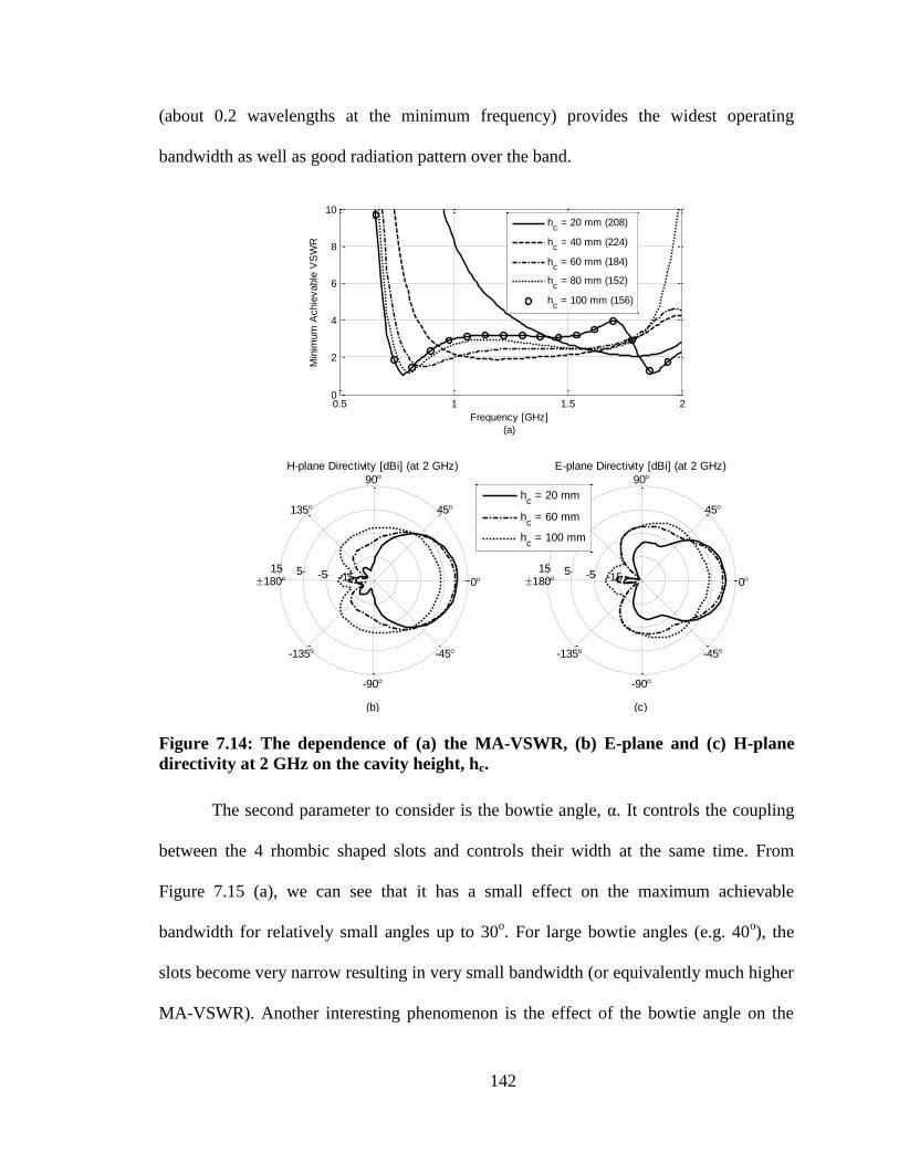
142

(about 0.2 wavelengths at the minimum frequency) provides the widest operating

bandwidth as well as good radiation pattern over the band.

Figure 7.14: The dependence of (a) the MA-VSWR, (b) E-plane and (c) H-plane

directivity at 2 GHz on the cavity height, hc.

The second parameter to consider is the bowtie angle, α. It controls the coupling

between the 4 rhombic shaped slots and controls their width at the same time. From

Figure 7.15 (a), we can see that it has a small effect on the maximum achievable

bandwidth for relatively small angles up to 30o. For large bowtie angles (e.g. 40

o), the

slots become very narrow resulting in very small bandwidth (or equivalently much higher

MA-VSWR). Another interesting phenomenon is the effect of the bowtie angle on the

0.5 1 1.5 20

2

4

6

8

10

Frequency [GHz]

(a)

Min

imum

Achie

vable

VS

WR

hc = 20 mm (208)

hc = 40 mm (224)

hc = 60 mm (184)

hc = 80 mm (152)

hc = 100 mm (156)

(b)

H-plane Directivity [dBi] (at 2 GHz)

-15-5515

0

45

90

135

180

-135

-90

-45

(c)

E-plane Directivity [dBi] (at 2 GHz)

-15-5515

0

45

90

135

180

-135

-90

-45

hc = 20 mm

hc = 60 mm

hc = 100 mm

143

required feed line characteristic impedance for optimum matching. Increasing the bowtie

angle (decreasing the slot angles) results in a reduction of the input impedance at the

antenna terminals. This is can be explained by noting that the feed port impedance can be

viewed as the parallel combination of the two perpendicular bowtie shaped tapered slot

lines terminated with inductive trace. When a standing wave is excited on these lines, it

excites the TE10 and TE01 modes in the cavity which are then radiated. Increasing the

slots’ angles corresponds to narrowing the slot line thus reducing its characteristic

impedance and reducing the input impedance at the antenna ports. Depending on the

chosen feeding structure, the appropriate bowtie angle can be selected.

Figure 7.15: Effect of the bowtie angle on the (a) MA-VSWR and (b) the required

characteristic impedance of the feed line for optimum VSWR.

The final parameter considered in this study is the feeding element width, We. The

effect of We on the MA-VSWR is shown in Figure 7.16 (a). Increasing We reduces the

intrinsic resonance of the exciting element allowing it to operate at lower frequencies as

shown in Figure 7.16 (a). However, since the cavity does not support frequencies

0.5 1 1.5 20

2

4

6

8

10

Frequency [GHz]

(a)

Min

imum

Achie

vable

VS

WR

= 10o (344)

= 20o (252)

= 30o (184)

= 40o (110)

10 20 30 40100

150

200

250

300

350

[Deg]

(b)

Required F

eed L

ine Z

0 [

]

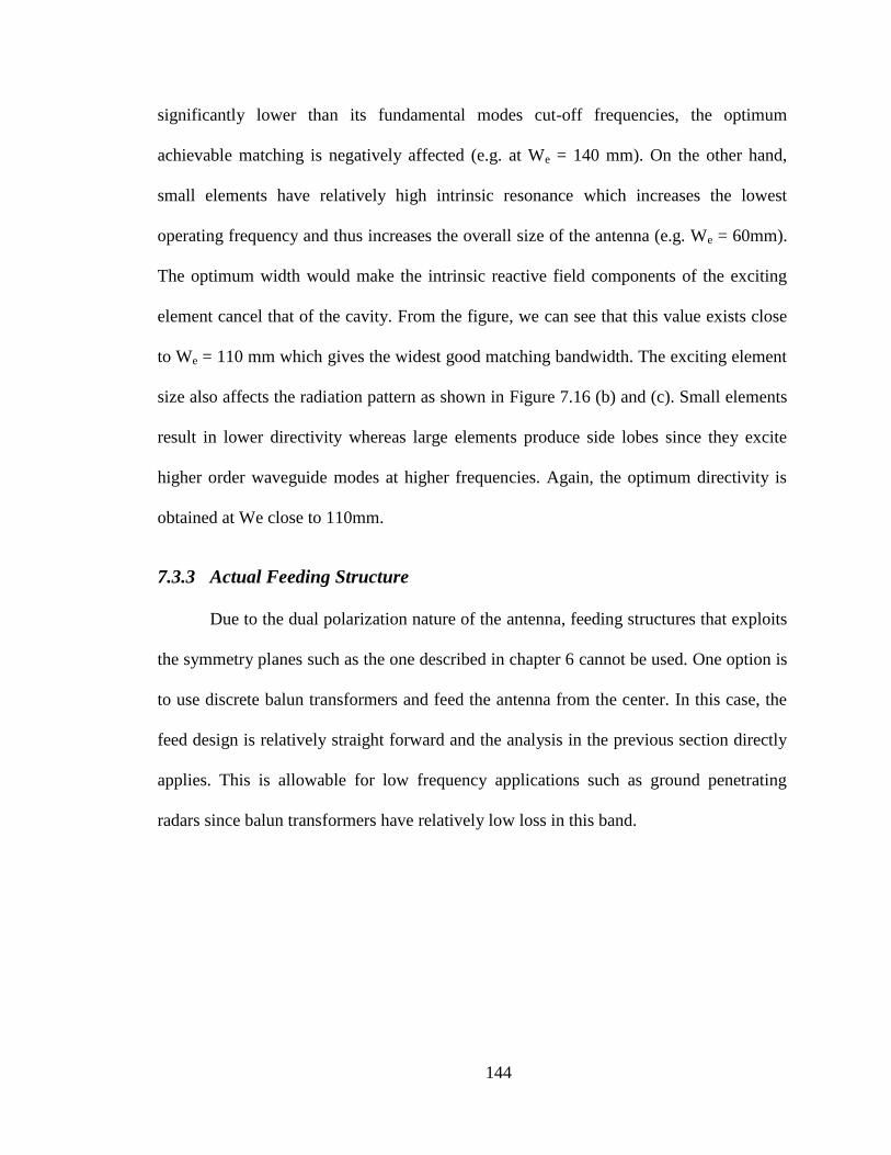
144

significantly lower than its fundamental modes cut-off frequencies, the optimum

achievable matching is negatively affected (e.g. at We = 140 mm). On the other hand,

small elements have relatively high intrinsic resonance which increases the lowest

operating frequency and thus increases the overall size of the antenna (e.g. We = 60mm).

The optimum width would make the intrinsic reactive field components of the exciting

element cancel that of the cavity. From the figure, we can see that this value exists close

to We = 110 mm which gives the widest good matching bandwidth. The exciting element

size also affects the radiation pattern as shown in Figure 7.16 (b) and (c). Small elements

result in lower directivity whereas large elements produce side lobes since they excite

higher order waveguide modes at higher frequencies. Again, the optimum directivity is

obtained at We close to 110mm.

7.3.3 Actual Feeding Structure

Due to the dual polarization nature of the antenna, feeding structures that exploits

the symmetry planes such as the one described in chapter 6 cannot be used. One option is

to use discrete balun transformers and feed the antenna from the center. In this case, the

feed design is relatively straight forward and the analysis in the previous section directly

applies. This is allowable for low frequency applications such as ground penetrating

radars since balun transformers have relatively low loss in this band.

145

Figure 7.16: The effect of the feed element width on (a) the MA-VSWR and (b) the

E-plane and (c) H-plane radiation patterns.

However, in other applications, transmission line baluns are preferable either due

to the unavailability of low loss discrete balun transformers in the desired operating band

or to minimize the fabrication and assembly costs. For these applications, we present a

distributed balun in this section. We used semi-rigid coaxial cables and a multi-section

microstrip line feed as shown in Figure 7.17 (a) and (b). For each polarization, one of the

bowtie triangles acts as the microstrip line ground whereas the other triangle is connected

to the microstrip line end as shown in Figure 7.17 (b). This is helped by the fact that the

triangles sides near the cavity wall have small current density which allows their use as

0.5 1 1.5 20

2

4

6

8

10

Frequency [GHz]

(a)

Min

imum

Achie

vable

VS

WR

We = 60 mm (534)

We = 80 mm (252)

We = 100 mm (214)

We = 120 mm (164)

We = 140 mm (174)

(b)

H-plane Directivity [dBi] (at 2 GHz)

-15-5515

0

45

90

135

180

-135

-90

-45

(c)

E-plane Directivity [dBi] (at 2 GHz)

-15-5515

0

45

90

135

180

-135

-90

-45

We = 60 mm

We = 100 mm

We = 140 mm

146

baluns to suppress the undesired unbalanced currents on the outer shield of the coaxial

cable as described in [rahmatt samii AP magazine paper on UWB baluns]. Two vias are

used to connect the two halves of the ring together across the substrate. The multi-section

microstrip line is used to match the relatively high antenna impedance at the input

terminals (about 200 Ohms). The tapered microstrip line ground together with the back

cavity act as a balun to suppress the unbalanced currents on the outer shield of the coaxial

cable. The exciting element size had to be modified to accommodate the different feeding

technique, so its width, Wc, was reduced to 90mm. The substrate used is a 60mil

RO4003C and the microstrip section dimensions are: L1 = 21mm, W1 = 2mm and W2 =

0.5 mm. Due to the relatively short MS line section allowed when using this feeding

technique, the minimum frequency shifted from around 0.85 GHz to 1 GHz. The current

distribution on the antenna terminals for the horizontal polarization is shown in Figure

7.18 (a). We can see that the current distribution is very similar to that of the ideal case.

The electric field inside the cavity is also plotted in Figure 7.18 (b), where we can see

that it is slightly affected by the presence of the two coaxial cables but the general

distribution remains the same. This is due to the fact that the two cables are perpendicular

to the direction of the electric field. However, since the structure is no longer fully

symmetric, the isolation between the two polarizations will decrease as will be shown in

the following section.

147

Feeding Semi-Rigid Coaxial Cables

Multi-section MS line

Top

Top

Bottom

L1W2

W1

Via

Via

(a) (b)

Figure 7.17: The actual feeding structure using multi-section microstrip line, (a)

isometric view and (b) top view of the exciting element.

(a) (b)

Figure 7.18: (a) The current distribution on the exciting element and (b) the electric

field distribution inside the cavity at 1.5GHz when using the MS line feed.

To verify the correct operation of the feed, the radiation pattern of the antenna

was simulated and the results are shown in Figure 7.19 (a) and (b) in the E- and H-planes

for the vertical polarization. We can see that the pattern is symmetric in the H-plane

(perpendicular to the feed line) since the antenna structure is symmetric around that

plane. However, in the E-plane, the pattern is slightly squinted by about 4 degrees. This is

in part due to the asymmetric cavity structure in this plane (due to the presence of the

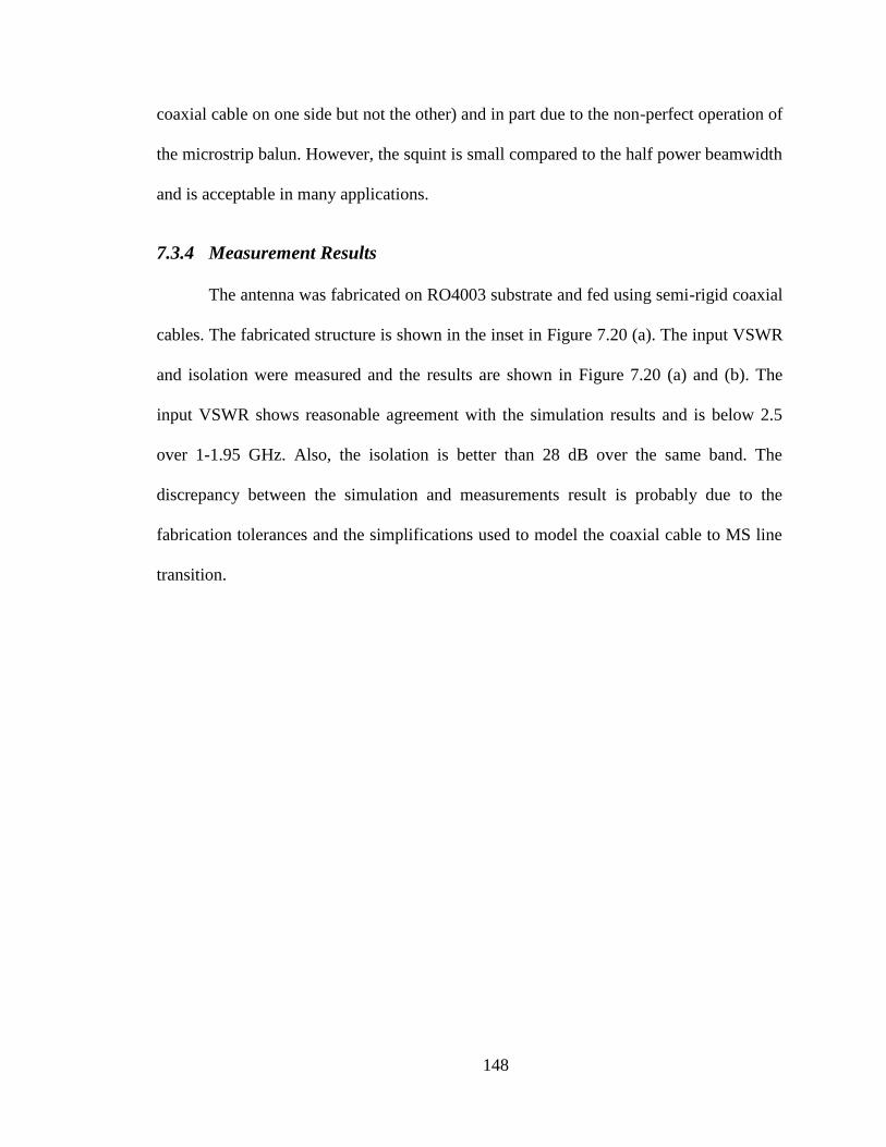
148

coaxial cable on one side but not the other) and in part due to the non-perfect operation of

the microstrip balun. However, the squint is small compared to the half power beamwidth

and is acceptable in many applications.


The antenna was fabricated on RO4003 substrate and fed using semi-rigid coaxial

cables. The fabricated structure is shown in the inset in Figure 7.20 (a). The input VSWR

and isolation were measured and the results are shown in Figure 7.20 (a) and (b). The

input VSWR shows reasonable agreement with the simulation results and is below 2.5

over 1-1.95 GHz. Also, the isolation is better than 28 dB over the same band. The

discrepancy between the simulation and measurements result is probably due to the

fabrication tolerances and the simplifications used to model the coaxial cable to MS line

transition.

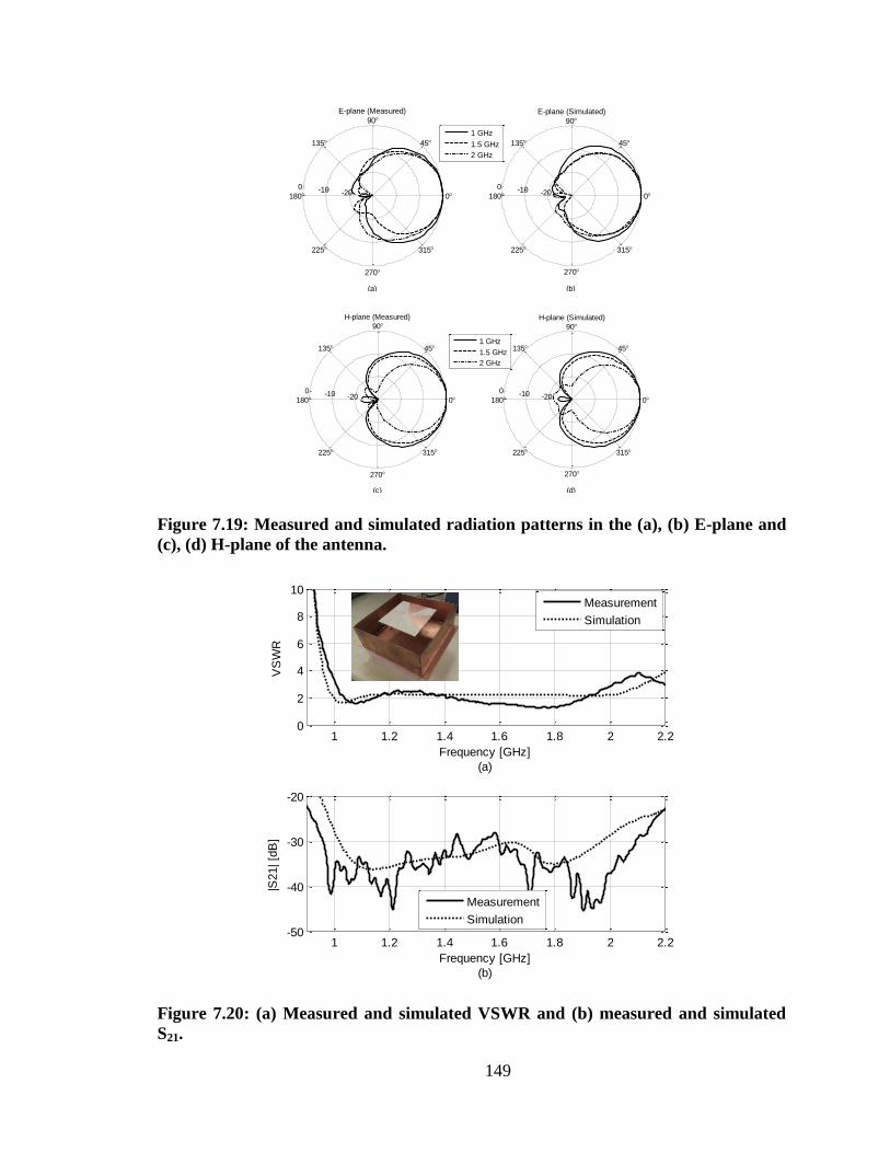
149

Figure 7.19: Measured and simulated radiation patterns in the (a), (b) E-plane and

(c), (d) H-plane of the antenna.

1 1.2 1.4 1.6 1.8 2 2.20

2

4

6

8

10

Frequency [GHz]

(a)

VS

WR

1 1.2 1.4 1.6 1.8 2 2.2-50

-40

-30

-20

Frequency [GHz]

(b)

|S21| [d

B]

Measurement

Simulation

Measurement

Simulation

Figure 7.20: (a) Measured and simulated VSWR and (b) measured and simulated

S21.

(a)

E-plane (Measured)

-20-100

0

45

90

135

180

225

270

315

(b)

E-plane (Simulated)

-20-100

0

45

90

135

180

225

270

315

1 GHz

1.5 GHz

2 GHz

(c)

H-plane (Measured)

-20-100

0

45

90

135

180

225

270

315

(d)

H-plane (Simulated)

-20-100

0

45

90

135

180

225

270

315

1 GHz

1.5 GHz

2 GHz

150

7.4 Conclusion

Three dual polarized antennas, based on the coupled sectorial loops antenna

principle, were presented. The first is a directional antenna for radar and communications

applications which utilizes asymmetrical loops and cavity backing to provide directional

radiation. It is shown that ultra wideband operation can be achieved and that the antenna

gain can be controlled by varying the cavity wall height. The second antenna is a

diversity antenna for communications application. It provides polarization and pattern

diversity. The design is fully planar and relatively compact. For this reason, it was

converted into a directional design by placing it inside a cavity with square cross-section.

Two of the proposed antennas were fabricated and measured and good agreement

between the simulation and measurements was observed.

151

Chapter 8

Very Low Profile UWB Antennas

The antennas presented in the previous chapters are relatively compact and can be

used for the GPR portion of the system. Depending on the aircraft used and the operating

frequency used, some of the previously presented antennas cannot be used for on-plane

mounting. This is because some of those antennas are relatively high profile which results

in significantly increased air drag if those antennas are mounted on the aircraft fuselage.

For this reason, we considered other antenna designs that (1) can be mounted on a ground

plane (an approximation of the plane fuselage), (2) have very low profile to reduce the air

drag and (3) have very wide bandwidth. In this chapter, we present two designs. One of

them is based on top loaded monopole antennas and the other design is based on a hybrid

TEM Horn – wide current loop. Both designs have very low profile (5.3% and 6.3% of

the minimum operating wavelength respectively) as well as very wide bandwidth (more

than one octave).

8.1 Very Low Profile UWB Monopole

8.1.1 Introduction

In certain low frequency applications, such as our VHF UWB InSAR system, it is

required to have a very low profile antenna operating at VHF frequencies that can be

mounted on a plane. In such situations, the antenna height from the plane fuselage has to

be as small as possible in order to minimize the air drag. This is also required in some

152

low frequency UWB military communication applications where it is again desired to

have low profile antenna to reduce the overall communication system size and weight.

Several UWB monopole structures have been proposed in the literature, such as

[57], [50]. They are planar structures and relatively easy to fabricate. However, their

height above the ground plane is relatively high (about 0.18λ0). Other antennas include

the monopole versions of biconical antennas such as [45] but they are still relatively high

profile and are even more difficult to fabricate. To reduce their size, it was found that

adding inductive shorting pins between the top and bottom creates a parallel resonance at

the low frequency end thus lowering the minimum operating frequency of the antenna

and consequently reduces the antenna size [5]. However, the structure presented in [58] is

not easy to fabricate, relatively heavy for low frequency implementations and its size is

still large (~0.17 λ0 for the dipole version) which is 38% higher profile than the design

presented in this paper.

Other monopole structures have also been presented in the literature such as [59].

These also suffer from relatively high profile (25% higher profile than our design), heavy

weight and require special fabrication for body of revolution structure which increases

their fabrication cost and required tolerances.

To address these issues we developed a new structure based on the shorted

biconical antenna. However, the new structure is fabricated using PCB technology which

allows us to have much better control on the feeding structure dimensions and allows for

much more precise tuning which allowed us to achieve a significantly smaller height of

0.053 λ0 compared to the previously mentioned structures. It is also relatively easy and

low cost to fabricate. In the following section, we will present the steps we used to reach

153

the final structure and the principle of operation. Next, we will present a parametric study

to show the effect of different antenna dimensions on its performance. Finally, we will

present the measurement results and the conclusion.


To design a low profile UWB antenna, we started with the top loaded monopole

antenna shown in Figure 8.1 (a). This structure is similar to a short monopolar biconical

antenna. However, this form is chosen over the conventional solid or wire biconical since

it can be easily fabricated using standard PCB technology and fabrication with good

repeatability can be achieved. Also it is very lightweight which is very important for the

low frequency applications considered where the antenna size is physically large.

However, as shown in Figure 8.2 (a) and (b), due to the very short height of this antenna,

the reactive component is very high at low frequencies and thus the antenna has to be

relatively tall to have good matching.

One technique to lower the minimum operating frequency is to use inductive shorting

pins to the ground which adds a low frequency resonance that nicely merges with the

high frequency biconical mode of the antenna as shown in Figure 8.2. Those pins can be

integrated into the fabricated feed PCBs as traces with controllable width as shown in

Figure 8.1 (b). As will be shown in the next section, the inductance of these inductive

traces control the first resonant frequency and can be easily controlled for optimum low

frequency matching.

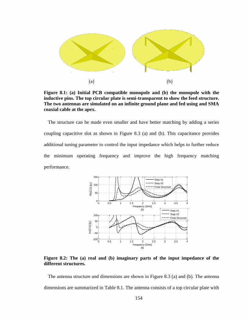
154

(a) (b)

Figure 8.1: (a) Initial PCB compatible monopole and (b) the monopole with the

inductive pins. The top circular plate is semi-transparent to show the feed structure.

The two antennas are simulated on an infinite ground plane and fed using and SMA

coaxial cable at the apex.

The structure can be made even smaller and have better matching by adding a series

coupling capacitive slot as shown in Figure 8.3 (a) and (b). This capacitance provides

additional tuning parameter to control the input impedance which helps to further reduce

the minimum operating frequency and improve the high frequency matching

performance.

Figure 8.2: The (a) real and (b) imaginary parts of the input impedance of the

different structures.

The antenna structure and dimensions are shown in Figure 8.3 (a) and (b). The antenna

dimensions are summarized in Table 8.1. The antenna consists of a top circular plate with

0 0.5 1 1.5 2 2.5 3 3.5 4-100

-50

0

50

100

Frequency [GHz]

(b)

ImZ

11

[ ]

0 0.5 1 1.5 2 2.5 3 3.5 40

50

100

150

Frequency [GHz]

(b)

ReZ

11

[ ]

Step #1

Step #2

Final Structure

Step #1

Step #2

Final Structure

155

an annular slot. The plate is connected to 4 feeding/shorting arms printed on two crossed

substrates. The shorting pins are responsible for the low frequency operation of the

antenna whereas the annular slot as well as the slots in the feeding arms help in

controlling the input impedance to match it to the feed.

(a)

(b)

Rp

tc tiRc

Ri

GND

hp

Figure 8.3: Antenna Structure (a) Isometric view and (b) side view with dimensions

(the substrate is not shown for clarity).

Table 8.1: Nominal Antenna Dimensions.

Rp Ri Rc

60 mm 55 mm 30 mm

tc ti hp h

1 mm 3.5 mm 1.5 mm 17.5 mm

The current distribution on one of the antenna fins at different frequencies is shown in

Figure 8.4. This figure indicates that at low frequencies, the electric current density is

very strong on the inductive traces. This is expected since the low frequency operation of

the antenna is attributed to them. As the frequency increases, the currents on these traces

become relatively small indicating that they no longer contribute much to the radiation. In

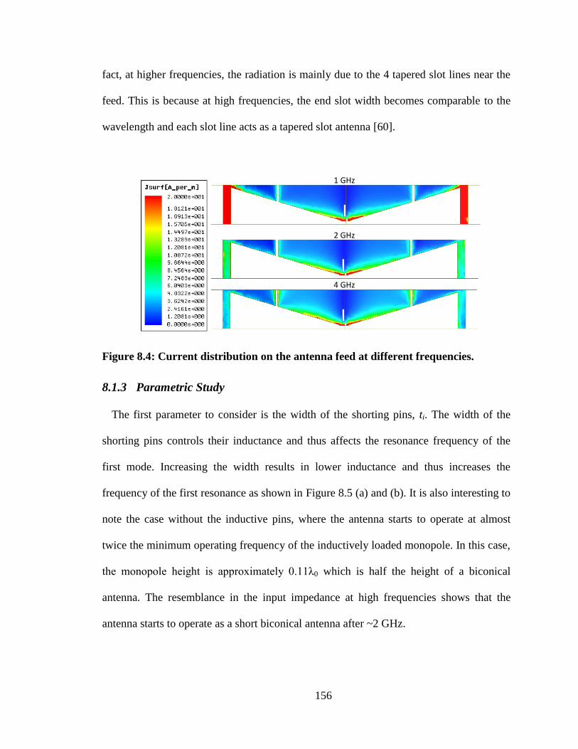
156

fact, at higher frequencies, the radiation is mainly due to the 4 tapered slot lines near the

feed. This is because at high frequencies, the end slot width becomes comparable to the

wavelength and each slot line acts as a tapered slot antenna [60].

1 GHz

2 GHz

4 GHz

Figure 8.4: Current distribution on the antenna feed at different frequencies.


The first parameter to consider is the width of the shorting pins, ti. The width of the

shorting pins controls their inductance and thus affects the resonance frequency of the

first mode. Increasing the width results in lower inductance and thus increases the

frequency of the first resonance as shown in Figure 8.5 (a) and (b). It is also interesting to

note the case without the inductive pins, where the antenna starts to operate at almost

twice the minimum operating frequency of the inductively loaded monopole. In this case,

the monopole height is approximately 0.11λ0 which is half the height of a biconical

antenna. The resemblance in the input impedance at high frequencies shows that the

antenna starts to operate as a short biconical antenna after ~2 GHz.

157

Figure 8.5: The effect of the inductive pins width on the (a) input VSWR and (b) the

real part of the input impedance.

The second parameter is the antenna height, h shown in Figure 8.6 (a) and (b). As

expected, increasing the antenna height increases the real part of the input impedance at

low frequencies since increasing the length of inductive pins enhances the radiation from

them. It also decreases the minimum resonance frequency since increasing the length of

the inductive traces increases their inductance thus decreasing the first resonant

frequency. The high frequency matching is improves as well since increasing h increases

the size of the radiating aperture of the 4 tapered slot antennas.

0 0.5 1 1.5 2 2.5 3 3.5 40

2

4

6

Frequency [GHz]

(a)V

SW

R

0 0.5 1 1.5 2 2.5 3 3.5 40

50

100

150

Frequency [GHz]

(b)

ReZ

11

[ ]

No Pins

t=1.5mm

t=3.5mm

t=5.5mm

No Pins

t=1.5mm

t=3.5mm

t=5.5mm

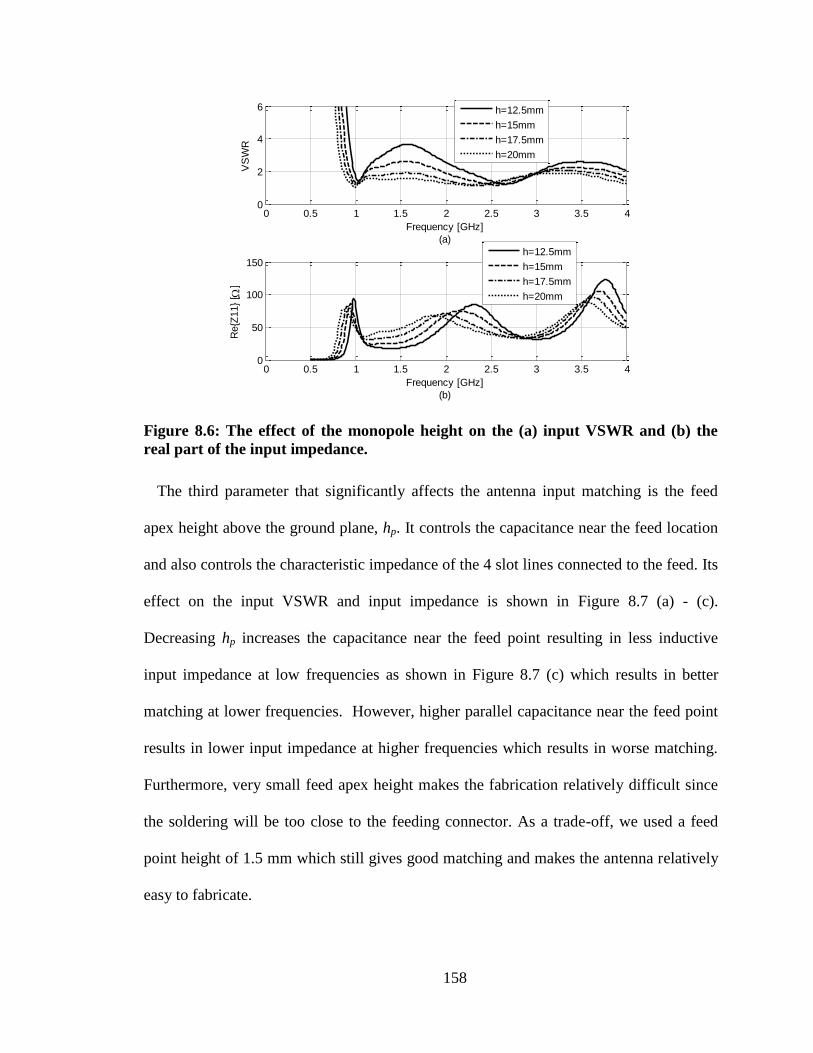
158

Figure 8.6: The effect of the monopole height on the (a) input VSWR and (b) the

real part of the input impedance.

The third parameter that significantly affects the antenna input matching is the feed

apex height above the ground plane, hp. It controls the capacitance near the feed location

and also controls the characteristic impedance of the 4 slot lines connected to the feed. Its

effect on the input VSWR and input impedance is shown in Figure 8.7 (a) - (c).

Decreasing hp increases the capacitance near the feed point resulting in less inductive

input impedance at low frequencies as shown in Figure 8.7 (c) which results in better

matching at lower frequencies. However, higher parallel capacitance near the feed point

results in lower input impedance at higher frequencies which results in worse matching.

Furthermore, very small feed apex height makes the fabrication relatively difficult since

the soldering will be too close to the feeding connector. As a trade-off, we used a feed

point height of 1.5 mm which still gives good matching and makes the antenna relatively

easy to fabricate.

0 0.5 1 1.5 2 2.5 3 3.5 40

2

4

6

Frequency [GHz]

(a)V

SW

R

0 0.5 1 1.5 2 2.5 3 3.5 40

50

100

150

Frequency [GHz]

(b)

ReZ

11

[ ]

h=12.5mm

h=15mm

h=17.5mm

h=20mm

h=12.5mm

h=15mm

h=17.5mm

h=20mm

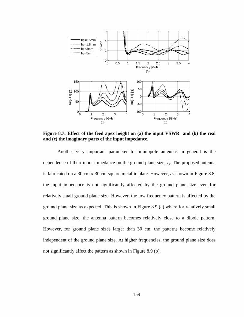
159

Figure 8.7: Effect of the feed apex height on (a) the input VSWR and (b) the real

and (c) the imaginary parts of the input impedance.

Another very important parameter for monopole antennas in general is the

dependence of their input impedance on the ground plane size, lg. The proposed antenna

is fabricated on a 30 cm x 30 cm square metallic plate. However, as shown in Figure 8.8,

the input impedance is not significantly affected by the ground plane size even for

relatively small ground plane size. However, the low frequency pattern is affected by the

ground plane size as expected. This is shown in Figure 8.9 (a) where for relatively small

ground plane size, the antenna pattern becomes relatively close to a dipole pattern.

However, for ground plane sizes larger than 30 cm, the patterns become relatively

independent of the ground plane size. At higher frequencies, the ground plane size does

not significantly affect the pattern as shown in Figure 8.9 (b).

0 0.5 1 1.5 2 2.5 3 3.5 40

50

100

150

Frequency [GHz]

(b)

ReZ

11

[ ]

hp=1mm

hp=2mm

hp=3mm

hp=4mm

hp=5mm

0 0.5 1 1.5 2 2.5 3 3.5 40

2

4

6

Frequency [GHz]

(a)

VS

WR

hp=0.5mm

hp=1.5mm

hp=3mm

hp=5mm

0 1 2 3 4-100

-50

0

50

100

Frequency [GHz]

(c)

ImZ

11

[ ]

0 1 2 3 40

50

100

150

Frequency [GHz]

(b)

ReZ

11

[ ]

160

Figure 8.8: Effect of the ground plane size, lg, on the input matching.

(a) (b)

Figure 8.9: Effect of the ground plane size on the E-plane pattern at (a) 1 GHz and

(b) 2 GHz.

8.1.4 Measurements Results

The antenna was fabricated on a 30 mil Rogers RO4003 substrate and fed using a

standard SMA coaxial cable. The fabricated antenna is shown in Figure 8.10 (a). It was

measured using an HP 8753D network analyzer and the simulated and measured VSWR

are shown in Figure 8.10 (b) where we can see very good agreement between the

simulation and measurements. The antenna has an input VSWR < 2 over the band 0.9 – 6

GHz corresponding to 148% relative bandwidth.

0 0.5 1 1.5 2 2.5 3 3.5 40

1

2

3

Frequency [GHz]

(a)

VS

WR

0 0.5 1 1.5 2 2.5 3 3.5 40

50

100

150

Frequency [GHz]

(b)

ReZ

11

[ ]

h=12.5mm

h=15mm

h=17.5mm

h=20mm

lg = 20cm

lg = 30cm

lg = 40cm

lg = 50cm

E-plane (1 GHz)

-20

-10

0

0

45

90

135

180

225

270

315

lg = 20cm

lg = 30cm

lg = 40cm

E-plane (2 GHz)

-20

-10

0

0

45

90

135

180

225

270

315

lg = 20cm

lg = 30cm

lg = 40cm

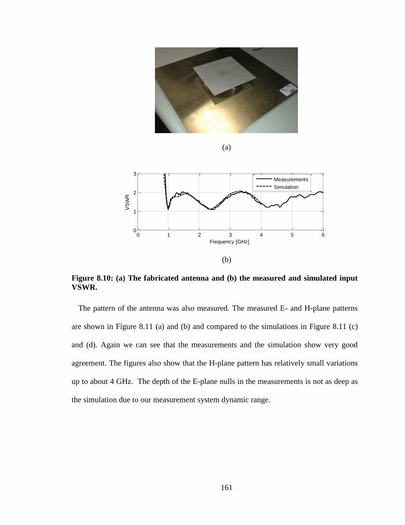
161

(a)

(b)

Figure 8.10: (a) The fabricated antenna and (b) the measured and simulated input

VSWR.

The pattern of the antenna was also measured. The measured E- and H-plane patterns

are shown in Figure 8.11 (a) and (b) and compared to the simulations in Figure 8.11 (c)

and (d). Again we can see that the measurements and the simulation show very good

agreement. The figures also show that the H-plane pattern has relatively small variations

up to about 4 GHz. The depth of the E-plane nulls in the measurements is not as deep as

the simulation due to our measurement system dynamic range.

0 1 2 3 4 5 60

1

2

3

Frequency [GHz]

VS

WR

Measurements

Simulation

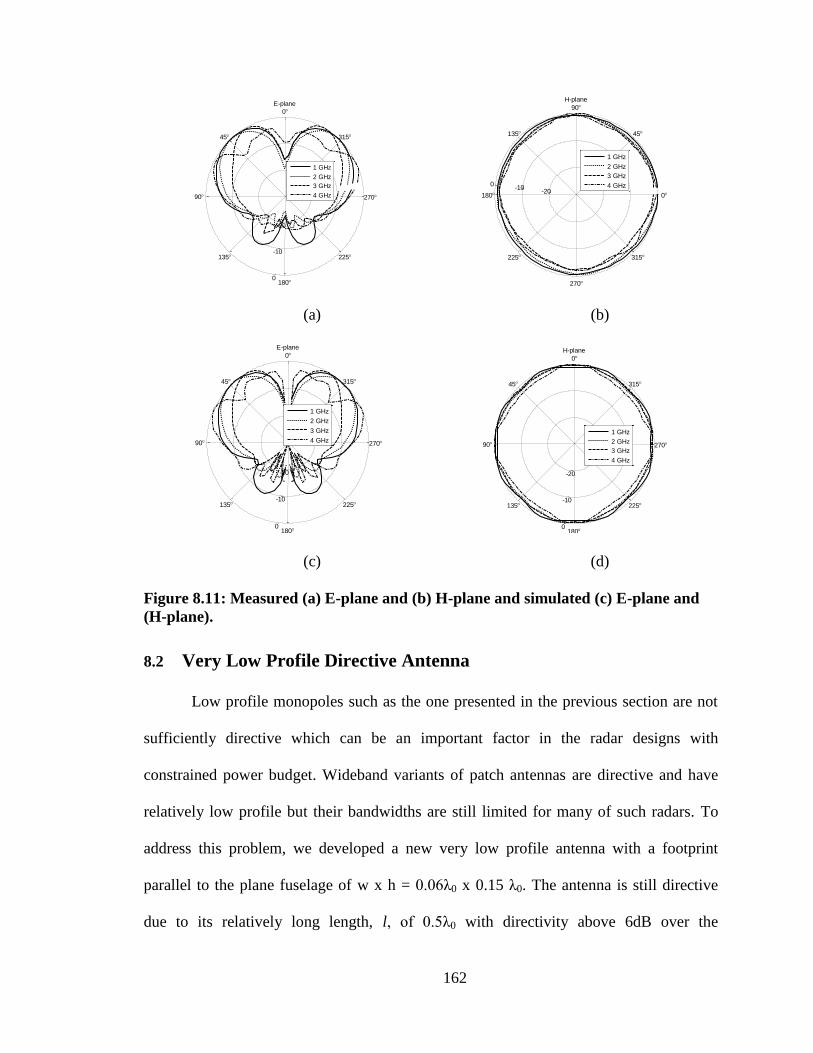
162

(a) (b)

(c) (d)

Figure 8.11: Measured (a) E-plane and (b) H-plane and simulated (c) E-plane and

(H-plane).

8.2 Very Low Profile Directive Antenna

Low profile monopoles such as the one presented in the previous section are not

sufficiently directive which can be an important factor in the radar designs with

constrained power budget. Wideband variants of patch antennas are directive and have

relatively low profile but their bandwidths are still limited for many of such radars. To

address this problem, we developed a new very low profile antenna with a footprint

parallel to the plane fuselage of w x h = 0.06λ0 x 0.15 λ0. The antenna is still directive

due to its relatively long length, l, of 0.5λ0 with directivity above 6dB over the

E-plane

-20

-10

0

0

45

90

135

180

225

270

315

1 GHz

2 GHz

3 GHz

4 GHz

H-plane

-20-10

0

0

45

90

135

180

225

270

315

1 GHz

2 GHz

3 GHz

4 GHz

E-plane

-20

-10

0

0

45

90

135

180

225

270

315

1 GHz

2 GHz

3 GHz

4 GHz

H-plane

-20

-10

0

0

45

90

135

180

225

270

315

1 GHz

2 GHz

3 GHz

4 GHz

163

bandwidth. It has good matching and directive pattern over about an octave of bandwidth.

The antenna is also relatively easy to fabricate and its dimensions can be tweaked to

achieve the desired directivity. In this section, we first present the antenna structure and

theory of operation, followed by a parametric study to show the effect of the different

parameters on the antenna performance. Then, the measurement results are presented.


Conventional UWB antennas mounted on a ground plane with direction of

maximum radiation normal to the ground plane typically have high profile. They can be

generally categorized into two categories: (1) a dipole in front of a ground plane and (2) a

traveling wave antenna (e.g. horn antenna). Placing a dipole in front of a ground plane

results in directional radiation if it is placed less than a quarter wavelength from the

ground plane [61]. However, a dipole cannot be placed too close to the ground plane;

otherwise wideband antenna matching becomes very difficult. This results in a relatively

high profile designs. On the other hand, traveling wave antennas have to be a significant

fraction (and even multiples) of the minimum operating wavelength which also results in

high profile design.

For these reasons, we decided to select a different approach to achieve very low

profile directive radiation. We chose a very low height half TEM horn as shown in Figure

8.12 (a). This antenna is oriented such that its traveling wave direction is parallel to the

ground plane which would result in direction of maximum radiation along the ground

plane for conventional TEM horns. However, since the aperture height of this antenna is

very small in the E-plane (YZ plane), its pattern is very wide in the E-plane as shown in

Figure 8.12 (b) and is relatively narrow in the other plane orthogonal to the ground plane

164

(XZ plane) since the antenna aperture is relatively long in this direction as shown in

Figure 8.12 (b). These types of patterns are actually desirable in airborne SAR

applications since it suppresses the Doppler ambiguities and allows wide swath coverage.

However, in spite of its desirable radiation characteristics, the antenna suffers from

resonant input impedance that makes matching it difficult over a wideband as shown in

Figure 8.12 (c).

15 cm

2 cm

4.8 cm

X

Z

Y

(a) (b)

(c)

Figure 8.12: (a) Short TEM horn dimensions, (b) its radiation patterns in the E- and

H- planes and (c) its input impedance.

To improve the input impedance matching, we used an inductive shorting trace as

shown in Figure 8.13 (a). This trace creates a resonance at lower frequencies that can be

shifted by controlling the inductance using the trace width, Ws, as shown in Figure 8.13

Radiation patterns at 1.5 GHz

-16

-12

-8

-4

0

0

45

90

135

180

225

270

315

E-plane

H-plane

0.5 1 1.5 2 2.5-100

0

100

200

Frequency [GHz]

Input

Impedance [

]

Real Part

Imaginary Part

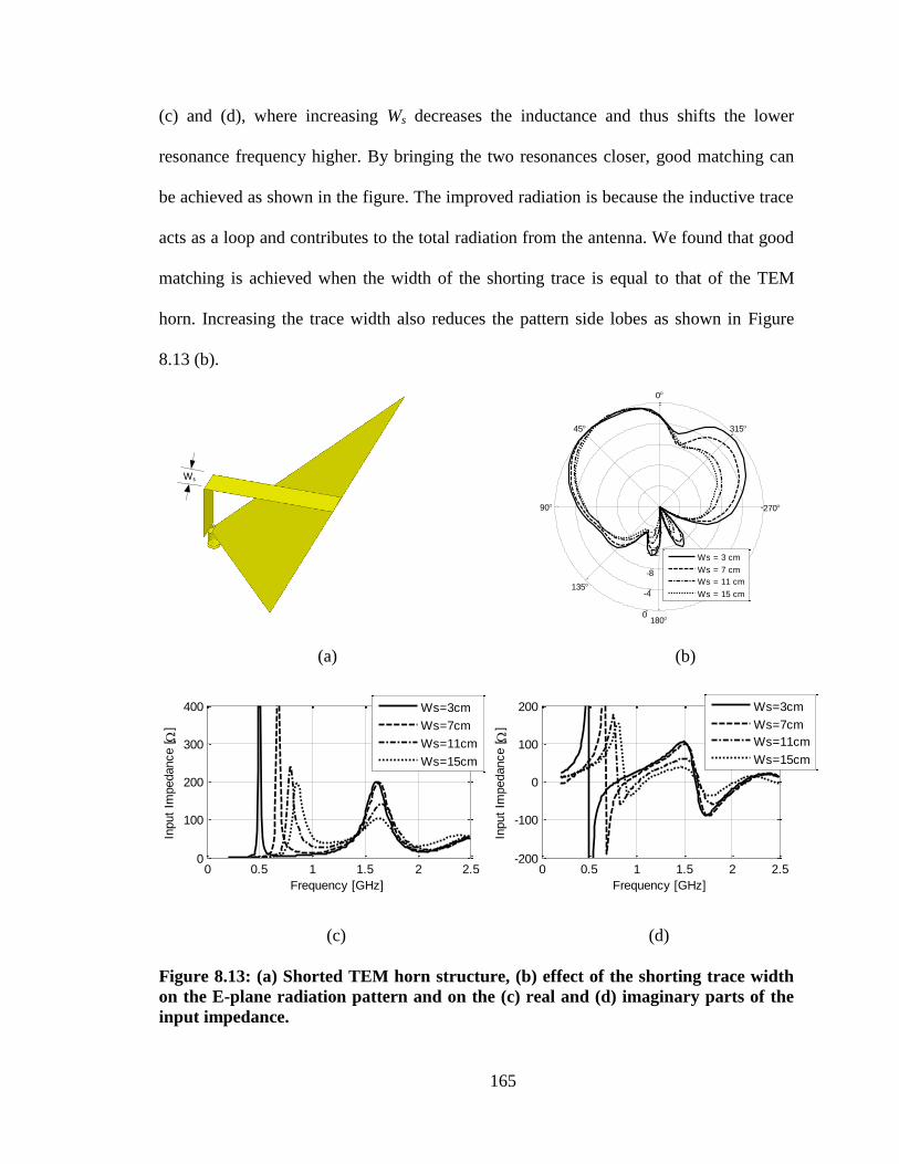
165

(c) and (d), where increasing Ws decreases the inductance and thus shifts the lower

resonance frequency higher. By bringing the two resonances closer, good matching can

be achieved as shown in the figure. The improved radiation is because the inductive trace

acts as a loop and contributes to the total radiation from the antenna. We found that good

matching is achieved when the width of the shorting trace is equal to that of the TEM

horn. Increasing the trace width also reduces the pattern side lobes as shown in Figure

8.13 (b).

Ws

(a) (b)

(c) (d)

Figure 8.13: (a) Shorted TEM horn structure, (b) effect of the shorting trace width

on the E-plane radiation pattern and on the (c) real and (d) imaginary parts of the

input impedance.

-16

-12

-8

-4

0

0

45

90

135

180

225

270

315

Ws = 3 cm

Ws = 7 cm

Ws = 11 cm

Ws = 15 cm

0 0.5 1 1.5 2 2.50

100

200

300

400

Frequency [GHz]

Input

Impedance [

]

Ws=3cm

Ws=7cm

Ws=11cm

Ws=15cm

0 0.5 1 1.5 2 2.5-200

-100

0

100

200

Frequency [GHz]

Input

Impedance [

]

Ws=3cm

Ws=7cm

Ws=11cm

Ws=15cm

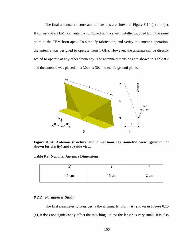
166

The final antenna structure and dimensions are shown in Figure 8.14 (a) and (b).

It consists of a TEM horn antenna combined with a sheet metallic loop fed from the same

point at the TEM horn apex. To simplify fabrication, and verify the antenna operation,

the antenna was designed to operate from 1 GHz. However, the antenna can be directly

scaled to operate at any other frequency. The antenna dimensions are shown in Table 8.2

and the antenna was placed on a 30cm x 30cm metallic ground plane.

l

w

h

Feed Position

(a) (b)

Gro

un

d

ZX

Y

Figure 8.14: Antenna structure and dimensions (a) isometric view (ground not

shown for clarity) and (b) side view.

Table 8.2: Nominal Antenna Dimensions.

W l h

4.7 cm 15 cm 2 cm


The first parameter to consider is the antenna length, l. As shown in Figure 8.15

(a), it does not significantly affect the matching, unless the length is very small. It is also

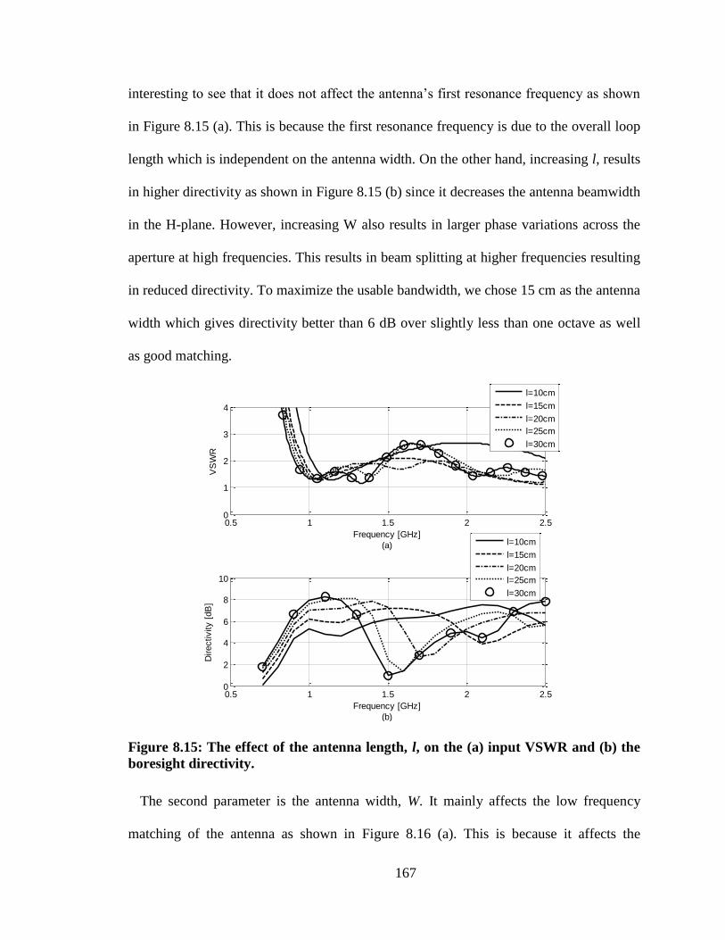
167

interesting to see that it does not affect the antenna’s first resonance frequency as shown

in Figure 8.15 (a). This is because the first resonance frequency is due to the overall loop

length which is independent on the antenna width. On the other hand, increasing l, results

in higher directivity as shown in Figure 8.15 (b) since it decreases the antenna beamwidth

in the H-plane. However, increasing W also results in larger phase variations across the

aperture at high frequencies. This results in beam splitting at higher frequencies resulting

in reduced directivity. To maximize the usable bandwidth, we chose 15 cm as the antenna

width which gives directivity better than 6 dB over slightly less than one octave as well

as good matching.

Figure 8.15: The effect of the antenna length, l, on the (a) input VSWR and (b) the

boresight directivity.

The second parameter is the antenna width, W. It mainly affects the low frequency

matching of the antenna as shown in Figure 8.16 (a). This is because it affects the

0.5 1 1.5 2 2.50

1

2

3

4

Frequency [GHz]

(a)

VS

WR

l=10cm

l=15cm

l=20cm

l=25cm

l=30cm

0.5 1 1.5 2 2.50

2

4

6

8

10

Frequency [GHz]

(b)

Directivity [

dB

]

l=10cm

l=15cm

l=20cm

l=25cm

l=30cm

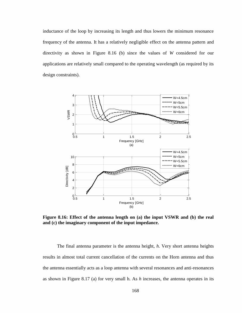
168

inductance of the loop by increasing its length and thus lowers the minimum resonance

frequency of the antenna. It has a relatively negligible effect on the antenna pattern and

directivity as shown in Figure 8.16 (b) since the values of W considered for our

applications are relatively small compared to the operating wavelength (as required by its

design constraints).

Figure 8.16: Effect of the antenna length on (a) the input VSWR and (b) the real

and (c) the imaginary component of the input impedance.

The final antenna parameter is the antenna height, h. Very short antenna heights

results in almost total current cancellation of the currents on the Horn antenna and thus

the antenna essentially acts as a loop antenna with several resonances and anti-resonances

as shown in Figure 8.17 (a) for very small h. As h increases, the antenna operates in its

0.5 1 1.5 2 2.50

1

2

3

4

Frequency [GHz]

(a)

VS

WR

W=4.5cm

W=5cm

W=5.5cm

W=6cm

0.5 1 1.5 2 2.50

2

4

6

8

10

Frequency [GHz]

(b)

Directivity [

dB

]

W=4.5cm

W=5cm

W=5.5cm

W=6cm

169

desired mode of a combined TEM horn and a loop antenna. h does not significantly affect

the boresight directivity except at very high frequencies as shown in Figure 8.17 (b).

Figure 8.17: Effect of the antenna height on the antenna's (a) input VSWR and (b)

real and (c) imaginary components of the input impedance.


The antenna was fabricated on a 10mil Rogers RO4003C substrate and placed on

a 30cm x 30cm metallic ground plane as shown in Figure 8.18 (a). The antenna input

impedance was measured and the results are shown in Figure 8.18 (b) where we can see

very good agreement between the measurements and the simulation.

0.5 1 1.5 2 2.50

1

2

3

4

Frequency [GHz]

(a)

VS

WR

0.5 1 1.5 2 2.50

2

4

6

8

10

Frequency [GHz]

(b)

Directivity [

dB

]

h=0.5cm

h=1.5cm

h=2cm

h=2.5cm

h=3cm

h=0.5cm

h=1.5cm

h=2cm

h=2.5cm

h=3cm

170

(a)

(b)

Figure 8.18: (a) A photo of the fabricated antenna and (b) the measured and the

simulated input VSWR.

The antenna co-pol pattern was also measured in the E- and H-planes as shown in

Figure 8.19 (a)-(d). From the two figures, we can see very good agreement between the

simulated and measured patterns.

0 0.5 1 1.5 2 2.5 3 3.50

1

2

3

4

5

Frequency [GHz]

VS

WR

Measurements

Simulation

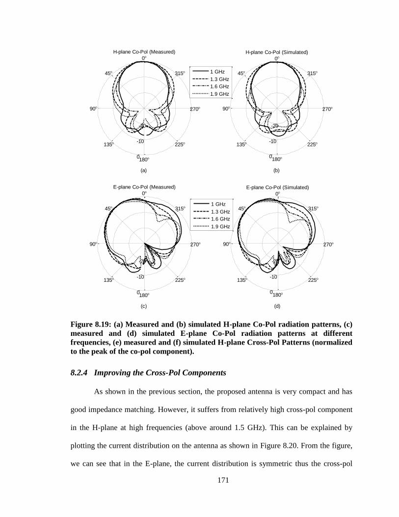
171

Figure 8.19: (a) Measured and (b) simulated H-plane Co-Pol radiation patterns, (c)

measured and (d) simulated E-plane Co-Pol radiation patterns at different

frequencies, (e) measured and (f) simulated H-plane Cross-Pol Patterns (normalized

to the peak of the co-pol component).

8.2.4 Improving the Cross-Pol Components

As shown in the previous section, the proposed antenna is very compact and has

good impedance matching. However, it suffers from relatively high cross-pol component

in the H-plane at high frequencies (above around 1.5 GHz). This can be explained by

plotting the current distribution on the antenna as shown in Figure 8.20. From the figure,

we can see that in the E-plane, the current distribution is symmetric thus the cross-pol

(a)

H-plane Co-Pol (Measured)

-20

-10

0

0

45

90

135

180

225

270

315

(b)

H-plane Co-Pol (Simulated)

-20

-10

0

0

45

90

135

180

225

270

3151 GHz

1.3 GHz

1.6 GHz

1.9 GHz

(c)

E-plane Co-Pol (Measured)

-20

-10

0

0

45

90

135

180

225

270

315

(d)

E-plane Co-Pol (Simulated)

-20

-10

0

0

45

90

135

180

225

270

3151 GHz

1.3 GHz

1.6 GHz

1.9 GHz

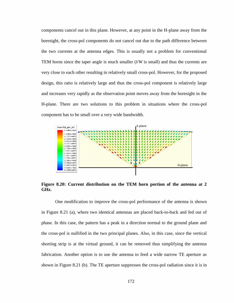
172

components cancel out in this plane. However, at any point in the H-plane away from the

boresight, the cross-pol components do not cancel out due to the path difference between

the two currents at the antenna edges. This is usually not a problem for conventional

TEM horns since the taper angle is much smaller (l/W is small) and thus the currents are

very close to each other resulting in relatively small cross-pol. However, for the proposed

design, this ratio is relatively large and thus the cross-pol component is relatively large

and increases very rapidly as the observation point moves away from the boresight in the

H-plane. There are two solutions to this problem in situations where the cross-pol

component has to be small over a very wide bandwidth.

E-plane

H-plane

Figure 8.20: Current distribution on the TEM horn portion of the antenna at 2

GHz.

One modification to improve the cross-pol performance of the antenna is shown

in Figure 8.21 (a), where two identical antennas are placed back-to-back and fed out of

phase. In this case, the pattern has a peak in a direction normal to the ground plane and

the cross-pol is nullified in the two principal planes. Also, in this case, since the vertical

shorting strip is at the virtual ground, it can be removed thus simplifying the antenna

fabrication. Another option is to use the antenna to feed a wide narrow TE aperture as

shown in Figure 8.21 (b). The TE aperture suppresses the cross-pol radiation since it is in

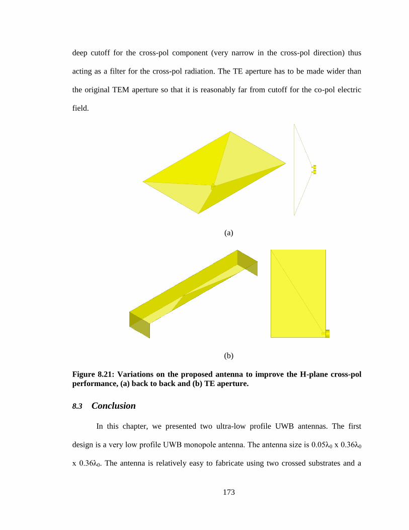
173

deep cutoff for the cross-pol component (very narrow in the cross-pol direction) thus

acting as a filter for the cross-pol radiation. The TE aperture has to be made wider than

the original TEM aperture so that it is reasonably far from cutoff for the co-pol electric

field.

(a)

(b)

Figure 8.21: Variations on the proposed antenna to improve the H-plane cross-pol

performance, (a) back to back and (b) TE aperture.

8.3 Conclusion

In this chapter, we presented two ultra-low profile UWB antennas. The first

design is a very low profile UWB monopole antenna. The antenna size is 0.05λ0 x 0.36λ0

x 0.36λ0. The antenna is relatively easy to fabricate using two crossed substrates and a

174

top substrate. The effects of the different antenna dimensions on the performance are

investigated. Of particular importance in monopole designs is the effect of the ground

plane. It was found that for this design, the ground plane does not have significant effect

on the input impedance matching and mainly affects the radiation patterns at lower

frequencies. A prototype antenna was fabricated and measured. The measured results

agree very well with the simulations where it is shown that the antenna operates over 0.9-

6 GHz with VSWR < 2. Also, as well as an omnidirectional pattern over more than two

octaves is observed. This antenna can be very useful in many low frequency radars and

military communications applications.

The monopole antenna presented have low profile and is relatively compact.

However, when placed on a plane fuselage for SAR ground imaging applications,

approximately half of the radiated power is wasted away towards the atmosphere which

can be a problem in some SAR applications that have constrained power budget. To

address this problem, we presented a directive design based on shorted short TEM horn.

The proposed antenna height is 0.063λ0 and has good matching and radiation

characteristics over more than an octave. It is based on the principle of an inductively

shorted TEM horn. However, unlike the standard TEM horn structures, the proposed

structure is designed to enhance the radiation in a direction perpendicular to the TEM

horn axis. This limits the maximum pattern bandwidth to about one octave but allows the

antenna height along the direction of maximum radiation to be very small. The antenna

was fabricated and measured. The measured results agreed well with the simulation

results and both showed that the antenna can operate over 1 – 2 GHz with good radiation

and matching performance within the fabrication tolerances. The antenna had relatively

175

high cross-pol component above around 1.5 GHz, and two design modifications were

proposed to address this problem.

176

Chapter 9

Conclusion and Future Work

9.1 Conclusions

In this thesis, we considered the problem of subsurface remote sensing in deserts

and arid regions. This problem has several aspects; it requires the study of the surface,

subsurface and volumetric scattering phenomena. The use of low frequency to allow

penetration through the top layer resulted in some additional system complexity due to

antenna size and the required wide relative bandwidth to achieve good spatial resolution.

9.1.1 Scattering Phenomena

The problem of subsurface scattering from arbitrarily two layers rough surfaces is

very complex and is still undergoing active research. This makes the inverse problem of

estimating the height of each layer using radar data significantly more complex. To

overcome this issue, we chose to use the two frequency extremes. At low frequencies

(VHF), the scattering from the top surface (sand surface) is negligible since the surface

undulations are much smaller than the wavelength at these frequencies. At high

frequencies (Ka), the surface and volumetric scattering from the top layer is dominant

and due to the high attenuation, the scattering from the bottom surface is negligible. This

lead to the simplified scattering model used for the forward and the inverse problem.

177

9.1.2 Subsurface Processing

For the Ka InSAR, the processing is relatively straightforward. However, for the

VHF InSAR, it was shown that conventional processing cannot be directly used due to

the refraction and propagation through the top layer. This lead to two main problems:

image distortion and inaccurate subsurface height estimation. Image distortion consisted

of SAR image azimuth defocusing as well as geometric distortion due to the top surface

undulations. It was also shown that range defocusing is relatively negligible due to the

relatively low loss of the sand at VHF frequencies.

9.1.3 Inversion Algorithm

If the top surface height is known, the subsurface height can be uniquely

identified using the VHF InSAR data. Thus we developed a new inversion algorithm that

utilizes the top surface topography map obtained from the Ka InSAR and the VHF

InSAR data to obtain the subsurface height. The inversion algorithm is physics based and

iteratively solves the nonlinear equations describing the propagation through the top

layer. It was shown to work in several top and bottom layer scenarios. The sensitivity of

the algorithm to systematic, measurement and environmental errors were also analyzed.

Of which, it is worth noting that the height error due to small variations in the sand

dielectric constant is relatively small which means that the algorithm can still provide

good results for slightly inhomogeneous layers. The algorithm was verified using 2D and

3D simulations as well as scaled model measurements in the lab.

178

9.1.4 Image Correction Algorithm

Several image distortion effects were observed in the obtained subsurface InSAR

images. As mentioned, they include SAR image defocusing as well as geometric

distortion. In order to correct for these effects, both the top surface topography and the

bottom surface topography have to be known. We noticed that the SAR image does not

suffer significant defocusing when the integration angle is small (low resolution) and the

defocusing gets progressively more pronounced as the integration angle increases (higher

resolution). Thus, we considered an iterative approach, initially focusing using small

integration angle thus producing two accurate albeit low resolution SAR images. The two

images are then used to obtain the subsurface height using the developed inversion

algorithm. The two raw images are then refocused on the correct subsurface height. The

process is repeated until the largest integration angle is used. The refocusing process can

be extremely time consuming due to the large number of nonlinear equations required to

describe the propagation through the top layer. Thus, we developed a fast subsurface

SAR simulator and processor based on 3D interpolation. Other issues such as the

estimation of the caustic surfaces and their effect on the image were also discussed. The

algorithm was verified using 3D simulations of realistic sand dunes and using scaled

model measurements in the lab.

9.1.5 Compact UWB Antennas

One of the major practical issues that appeared during the subsurface InSAR

development is the design of compact wideband antennas for both the VHF InSAR and

for the ground penetrating radar used to obtain the ground control points required for the

phase unwrapping. Due to the low operating frequency and consequently the large

179

operating wavelength, the antenna size becomes relatively large which causes practical

limitations for plane mounting as well as in GPR vehicle mounting. This is a very

common in many other applications as well such as see through wall radars where the

operating frequency has to be low to allow penetration through lossy concrete walls. It

also exists in many UWB and MIMO communication applications where compact

antennas are also desired. For these reasons, we chose to address this problem in detail

and developed a number of UWB antennas for InSAR and GPR applications. The

developed antennas can also be used in the mentioned see through wall radar and

communication applications.

9.1.6 Linearly Polarized UWB Antennas

We developed a number of linearly polarized antennas based on the coupled

sectorial loops antenna (CSLA) principle. First, we showed that using the fact that the

magnetic field is circulating around the antenna; we could reduce the antenna maximum

dimension by 50%. Next, we noticed that the antenna pattern became directional at

higher frequencies especially when combining the CSLA with a tapered slot antenna.

Using this frequency dependent directivity, we combined the CSLA with a corner

reflector. The resulting antenna showed very good matching and radiation pattern over a

bandwidth of more than two octaves as well as very good time domain characteristics.

Compared to a ridged horn antenna, the new structure provides comparable gain while

being almost 1/8th

the size.

The previous design requires the presence of a ground plane which makes it

unsuitable in some radar and communication applications. Thus, we developed another

directive UWB antenna based on open ended rectangular waveguide antennas

180

(OERWGA). Conventional OERWGAs are narrow band due to the resonant feeds

typically used. They are also typically long and bulky since the waveguide length is

required to suppress the higher order modes excited by the feed. To overcome these

limitations, we used a bowtie feed which can excite an aperture field distribution very

similar to that of the fundamental mode of the rectangular waveguide using very short

waveguide section and over an ultrawide band. The antenna had good matching and

radiation pattern over a relative bandwidth of 3.3:1 as well as good time domain

characteristics. It had 1.5dB less gain than a ridged horn antenna while being less than

1/8th

the size and 1/4th

the height.

9.1.7 High Isolation Antenna Pair

In some applications such as GPR, see through wall radar as well as MIMO

communications, two or more antennas are used. In these situations, it is desired to have

the two antennas electrically close to reduce the overall system size and weight.

However, placing two antennas very close to each other results in strong mutual coupling

between them. This causes increased quantization noise in radar applications. Also, in

communication applications, this coupling increases the correlation between the received

signals at the two antennas which reduces the effective number of channels (and

consequently the maximum data throughput). To address this problem, we developed a

transmit/receive antenna pair with directive pattern and isolation better than 20 dB over

an octave of bandwidth. The high isolation is due to the use of an isolating structure

consisting of a parallel plate waveguide and a rectangular waveguide.

181

9.1.8 Dual Polarized Antennas

In some radar applications, additional polarization provides extra information that

can be used in target recognition and/or clutter reduction. In communication applications,

it can increase the channel capacity and/or improve the received signal to noise ratio due

to polarization diversity. Thus, we developed a number of dual polarized antennas based

on the coupled sectorial loops. Two designs are directional for radar and communication

applications. An additional dual polarized diversity antenna was designed for

communications applications.

9.1.9 Very Low-Profile Antennas

For airborne applications, the antenna’s profile from the plane fuselage becomes

an important issue. In some applications, the antenna can be flushed into the plane

fuselage and in such situations some of the presented antennas can be used. However, in

other applications, the antenna has to be mounted on the plane fuselage and the profile of

the antenna is desired to be as low as possible. For these situations, we developed two

very low profile antennas, one of them is based on the inductively loaded biconical

antenna. This antenna is omni-directional and has a very low profile of 0.053 of the

minimum operating wavelength. However, about half of the power is wasted into the

atmosphere when it is side mounted on an airplane which can be important in some

power budget limited SAR designs. The other low profile antenna is directive and thus

does not suffer this problem. It has slightly higher profile at 0.064 of the minimum

operating frequency and a narrow beam in the H-plane which allows relatively wide

swath coverage with reduced Doppler ambiguities. The original antenna has relatively

182

high cross-pol at higher frequencies and thus two different variations on the original

design are presented to address this issue.

9.2 Future Work

9.2.1 Scattering from Targets under a Rough Surface

In this thesis, the main goal was the estimation of the topography of relatively

deep bedrock (tens of meters). In some applications, such as mine detection, it is desired

to detect relatively shallow targets with higher ground resolution. In such situations, the

frequency used will be higher (UHF range) to allow for wider bandwidth and thus higher

resolution. In such situations, the surface roughness might become significant and the

interaction between the subsurface targets and the top interface becomes important. The

InSAR correction algorithm can also be used to accurately register the correct location of

these targets.

9.2.2 Scattering from Large Dunes

In the analysis performed in this thesis, the scattering from the top surface is

neglected. This is true for most parts of the map except for the dune peak curves where

the surface slope changes relatively fast. The method suggested in this thesis is to detect

these parts of the map using the Ka-InSAR map and remove it from the VHF-InSAR

map. However, depending on the peak direction and the radar incidence angle, the actual

scattering from it might not be very strong. Using high frequency techniques with the top

surface map, the locations of the high scattering points can be estimated much more

accurately and maybe even subtracted from the radar signal.

183

9.2.3 Scattering and Propagation in Dense Random Media

The current theories for wave propagation in random media are based on either

the wave approach which is very computationally intensive and requires certain

approximations to make it computationally feasible. Some of these approximations are

not valid for dense random media such as sand. The other approach is based on radiative

transfer theory, which is much less computationally intensive. However, it requires the

knowledge of the phase and extinction matrices for the medium which are not

straightforward to obtain. This problem can be approached using a hybrid numerical and

radiative transfer model where a packing algorithm can be used to calculate the pair

distribution function and a numerical technique is used to compute the effective

permittivity of the dense medium using Mone-Carlo simulations as well as phase and

extinction matrices which are then employed in the radiative transfer formulation. Also,

the interaction between volume and surface scattering for natural surfaces should be

analyzed.

184

Bibliography

[1] Denham, L.R., "Seismic interpretation," Proceedings of the IEEE , vol.72, no.10, pp.

1255- 1265, Oct. 1984.

[2] C. S Bristow, S. D Bailey and N Lancaster, ―The sedimentary structure of linear

sand dunes‖, Nature, pp. 56-59, July 2000.

[3] A. P. Annan, ―GPR—History, trends, and future developments,‖ Subsurface Sens.

Technol. Appl., vol. 3, no. 4, pp. 253–270, Oct. 2002.

[4] D. L. Moffatt and R. J. Puskar, ―A subsurface electromagnetic pulse radar,‖

Geophysics, vol. 41, pp. 506-518, June 1976.

[5] H. Brunzell, ―Detection of shallowly buried objects using impulse radar,‖ IEEE

Trans. Geosci. Remote Sensing, vol. 37, pp. 875–886, May 1999.

[6] H. Hellsten, L. M. H. Ulander, A. Gustavsson and B. Larsson, ―Development of

VHF CARABAS II SAR,‖ in Proc. Radar Sensor Technology, SPIE vol. 2747,

Orlando, FL, April 8-9, 1996, pp. 48-60.

[7] Dehmollaian, M.; Sarabandi, K.; , "Refocusing Through Building Walls Using

Synthetic Aperture Radar," Geoscience and Remote Sensing, IEEE Transactions on ,

vol.46, no.6, pp.1589-1599, June 2008.

[8] M. Ghavami, LB Michael, and R. Kohno.

[9] http://en.wikipedia.org/wiki/Ground-penetrating_radar.

[10] Elsherbini, A.; Sarabandi, K.; , "Topography of sand covered bedrock using two-

frequency airborne interferometric SAR measurements," Geoscience and Remote

Sensing Symposium,2009 IEEE International, IGARSS 2009 , vol.2, no., pp.II-250-

II-253, 12-17 July 20.

[11] Elsherbini, A.; Sarabandi, K.; , "Mapping of Sand Layer Thickness in Deserts Using

SAR Interferometry," Geoscience and Remote Sensing, IEEE Transactions on ,

vol.48, no.9, pp.3550-3559, Sept. 2010.

[12] http://www.msss.com/mars_images/moc/8_10_99_releases/moc2_170/.

[13] http://science.nasa.gov/headlines/y2002/06dec_dunes.htm.

[14] Richards, M.A.; , "A Beginner's Guide to Interferometric SAR Concepts and Signal

Processing [AESS Tutorial IV]," Aerospace and Electronic Systems Magazine, IEEE

, vol.22, no.9, pp.5-29, Sept. 2007.

[15] C. Prati and F. Rocca, "Limits to the resolution of elevation maps from stereo SAR

images," Int. J. Remote Sensing 11, 2215-2235 (1990).

[16] Chevrel, M, Courtis, M and Weill, G ―The SPOT satellite remote sensing mission‖

Photogrammetric Eng. Remote Sensing Vol. 47, No 8 (1981) pp 1163-1171.

[17] Flood, M., 2001, Laser altimetry: from science to commercial LIDAR mapping.

185

Photogrammetric Engineering & Remote Sensing, 67(11), 1209-1217.

[18] Chu, L. J.; , "Physical Limitations of Omni‐Directional Antennas," Journal of

Applied Physics , vol.19, no.12, pp.1163-1175, Dec 1948.

[19] Geyi, W.; , "Physical limitations of antenna," Antennas and Propagation, IEEE

Transactions on , vol.51, no.8, pp. 2116- 2123, Aug. 2003.

[20] Dehmollaian, M.; Sarabandi, K.; , "Analytical, numerical, and experimental methods

for through-the-wall radar imaging," Acoustics, Speech and Signal Processing, 2008.

ICASSP 2008. IEEE International Conference on , vol., no., pp.5181-5184, March

31 2008-A.

[21] Mahfouz, M.R.; Cemin Zhang; Merkl, B.C.; Kuhn, M.J.; Fathy, A.E.; ,

"Investigation of High-Accuracy Indoor 3-D Positioning Using UWB Technology,"

Microwave Theory and Techniques, IEEE Transactions on , vol.56, no.6, pp.1316-

1330, June 2008.

[22] Elsherbini, A.; Cemin Zhang; Fathy, A.E.; Mahfouz, M.; , "Notch bandwidth and

filter order trade-offs in band-notched monopole antennas for UWB applications,"

Antennas and Propagation Society International Symposium, 2008. AP-S 2008.

IEEE , vol., no., pp.

[23] Rosen, P.A.; Hensley, S.; Joughin, I.R.; Li, F.K.; Madsen, S.N.; Rodriguez, E.;

Goldstein, R.M.; , "Synthetic aperture radar interferometry," Proceedings of the

IEEE , vol.88, no.3, pp.333-382, Mar 2000.

[24] DC Ghiglia and MD Pritt Two-Dimensional Phase Unwrapping: Theory, Algorithms

and Software, Wiley, Chichester, New York (1998).

[25] Zebker, H. A., R. M. Goldstein (1986), Topographic mapping from interferometric

synthetic aperture radar observations, J. Geophys. Res., 91, 4993-4999.

[26] A. Tabatabaeenejad and M. Moghaddam, "Bistatic scattering from three-

dimensional layered rough surfaces", Geoscience and Remote Sensing, IEEE

Transactions on , vol.44, no.8, pp.2102-2114, Aug. 2006.

[27] A. Nashashibi and K. Sarabandi, "Volume scattering from a layer of sand at Ka-

Band: Measurements and simulations," Antennas and Propagation Society

International Symposium, 2009. APSURSI '09. IEEE, pp.1-4, 1-5 June 2009.

[28] P. Paillou, S. Lopez, Y. Lasne, A. Rosenqvist and T. Farr, "Mapping subsurface

geology in Arid Africa using L-band SAR," Geoscience and Remote Sensing

Symposium, 2007. IGARSS 2007. IEEE International , pp.2685-2688, 23-28 July

2007.

[29] J. F. McCauley, G. G. Schaber, C. S. Breed, M. J. Grolier, C. V. Haynes, B. Issawi,

C. Elachi and R. Blom., ―Subsurface valleys and geoarchaeology of the eastern

Sahara revealed by Shuttle Radar,‖ Science, vol. 218, pp. 1004-1020, 1982.

[30] Ph. Paillou, A. Rosenqvist and T. Farr, ―A JERS-1 radar mosaic for subsurface

geology mapping in East Sahara,‖ Proc. IGARSS’03, Toulouse, France, July 2003.

[31] K. K. Williams, R. Greeley, "Radar attenuation by sand: laboratory measurements of

radar transmission," Geoscience and Remote Sensing, IEEE Transactions on ,

vol.39, no.11, pp.2521-2526, Nov 2001.

[32] A. K. Fung, Z. Li and K. S. Chen, ―Backscattering from a randomly rough dielectric

186

surface‖, IEEE Transactions on Geoscience and Remote Sensing, vol.30, no.2,

pp.356-369, Mar 1992.

[33] P. Beckman and A. Spizzichino, ―The scattering of electromagnetic waves from

rough surfaces‖, Oxford: Pergamon, 1963.

[34] L.M.H. Ulander et al, ―Development of the ultra-wideband LORA SAR operating in

the VHF/UHF-band,‖ in Proc. IGARSS’03, Toulouse, France, July 21-25, 2003, pp.

4268-4270.

[35] M.E. Davis, ―Technical challenges in ultra-wideband radar development for target

detection and terrain mapping,‖ in Proc. 1999 IEEE Radar Conference, Waltham,

MA, April 20-22, 1999, pp. 1-6.

[36] K. Sarabandi (PI), "Topography of Sand Covered Bedrock Using a Two-Frequency

Interforometric SAR Measurements", Technical Report, University of Michigan.

[37] L. M. Ulander, H. Hellsten and G. Stenstrom, ―Synthetic-aperture radar processing

using fast factorized back-projection‖, IEEE Transactions on Aerospace and

Electronic Systems, vol.39, no.3, pp. 760-776, July 2003.

[38] Jong-Sen Lee, K. W. Hoppel, S. A. Mango and A. R. Miller, ―Intensity and phase

statistics of multilook polarimetric and interferometric SAR imagery‖, IEEE

Transactions on Geoscience and Remote Sensing, vol.32, no.5, pp.1017-1028, Sep

1994.

[39] G. FRANCESCHETTI AND R. LANARI, Synthetic Aperture Radar Processing,

CRC Press, New York, 1999.

[40] Xuan Yu, Feng Li, Jingyi Yu. Image-space Caustics and Curvatures. In Proceedings

of 15th Pacific Conference on Computer Graphics and Applications, pp. 181-188,

2007.

[41] M. A. Shah, J. Konttinen, and S. Pattanaik. Caustics mapping: An image-space

technique for real-time caustics. IEEE Transactions on Visualization and Computer

Graphics, 13(2):272–280, 2007.

[42] A.J. Rosakis and A.T. Zehnder, On the method of caustics: an exact analysis based

on geometrical optics, Journal of Elasticity 4 (1985), pp. 347–367..

[43] M. Di Benedetto, T. Kaiser, D. Porcino, A. Molisch, and I. Opperman, UWB

Communication Systems A Comprehensive Overview. Hindawi Publising, May,

2006.

[44] H. Schantz, The art and science of ultrawideband antennas, Artech House, Boston,

2005.

[45] C. A. Balanis, Antenna Theory, 2nd Ed., John Wiley & Sons, Inc., New York, 1982,

pp. 214-217.

[46] Xue Ni Low; Zhi Ning Chen; See, T.S.P.; , "A UWB Dipole Antenna With

Enhanced Impedance and Gain Performance," Antennas and Propagation, IEEE

Transactions on , vol.57, no.10, pp.2959-2966, Oct. 2009.

[47] E. Gazit, ―Improved design of the Vivaldi antenna,‖ Proc.

[48] Adel Elsherbini et al., "UWB antipodal vivaldi antennas with protruded dielectric

rods for higher gain, symmetric patterns and minimal phase center variations," 2007

IEEE Antennas and Propagation International Symposium, pp. 1973-1976, June 200.

187

[49] Bruns, C.; Leuchtmann, P.; Vahldieck, R., "Analysis and Simulation of a 1-18-GHz

broadband double-ridged horn antenna," Electromagnetic Compatibility, IEEE

Transactions on , vol.45, no.1, pp. 55-60, Feb 2003.

[50] Behdad, N.; Sarabandi, K.; , "A compact antenna for ultrawide-band applications,"

Antennas and Propagation, IEEE Transactions on , vol.53, no.7, pp. 2185- 2192, July

2005.

[51] R. E. Collin, Field Theory of Guided Waves, 2nd ed. IEEE, New York, 1991.

[52] Blanch, S.; Romeu, J.; Corbella, I.; , "Exact representation of antenna system

diversity performance from input parameter description," Electronics Letters ,

vol.39, no.9, pp. 705- 707, 1 May 2003.

[53] Eide, E.S., "Ultra-wideband transmit/receive antenna pair for ground penetrating

radar," Microwaves, Antennas and Propagation, IEE Proceedings - , vol.147, no.3,

pp.231-235, Jun 2000.

[54] Mak, A.C.K.; Rowell, C.R.; Murch, R.D., "Isolation Enhancement Between Two

Closely Packed Antennas," Antennas and Propagation, IEEE Transactions on ,

vol.56, no.11, pp.3411-3419, Nov. 2008.

[55] Young Jun Song; Sarabandi, K.; , "Suppression of the mutual coupling between two

adjacent miniaturized antennas utilizing printed resonant circuits," Antennas and

Propagation Society International Symposium, 2009. APSURSI '09. IEEE , vol., no.,

pp.1-4, 1-.

[56] Adamiuk, G.; Beer, S.; Wiesbeck, W.; Zwick, T., "Dual-Orthogonal Polarized

Antenna for UWB-IR Technology," Antennas and Wireless Propagation Letters,

IEEE, vol. 8, pp. 981-984, 2009.

[57] Jianxin Liang; Chiau, C.C.; Xiaodong Chen; Parini, C.G.,"Study of a printed circular

disc monopole antenna for UWB systems," Antennas and Propagation, IEEE

Transactions on , vol.53, no.11, pp. 3500- 3504, Nov. 2005.

[58] Amert, A.K.; Whites, K.W.,"Miniaturization of the Biconical Antenna for

Ultrawideband Applications," Antennas and Propagation, IEEE Transactions on ,

vol.57, no.12, pp.3728-3735, Dec. 2009.

[59] Nakano, H.; Morishita, K.; Yamauchi, J.; , "Extremely Wide-band, Low-profile

BOR-SPR Antenna," Antenna Technology: Small Antennas and Novel

Metamaterials, 2008. iWAT 2008. International Workshop on , vol., no., pp.20-23,

4-6 March 2008.

[60] Schaubert, D.; Kollberg, E.; Korzeniowski, T.; Thungren, T.; Johansson, J.;

Yngvesson, K., "Endfire tapered slot antennas on dielectric substrates," Antennas

and Propagation, IEEE Transactions on , vol.33, no.12, pp. 1392- 1400, Dec 1985.

[61] Elsherbini, A.; Sarabandi, K.; , "Directive Coupled Sectorial Loops Antenna for

Ultrawideband Applications," Antennas and Wireless Propagation Letters, IEEE ,

vol.8, no., pp.576-579, 2009.

radar remote sensing of arid regions - university of michigan

Documents