racial, educational, and religious endogamy in the united states

Racial, Educational, and Religious Endogamy

In the United States:

A Comparative Historical Perspective

Running Head: Comparative Endogamy

Michael J. Rosenfeld*

Dept. Sociology

Stanford University

Published in and Copyright owned by Social Forces 2008

volume 87, number 1, p. 1-32 (lead article)

* Department of Sociology, Stanford University, 450 Serra Mall, Bldg 120, Stanford, CA 94305. Email [email protected]. Website: www.stanford.edu/~mrosenfe. Thanks are due to Byung-Soo Kim for help with preliminary data analysis, to Emily Ryo, Christine Schwartz, and David Grusky for their many helpful comments, and to the Russell Sage Foundation for their support.

Abstract: This paper draws broad comparisons between marriage patterns by race, by education, and by religion in the U.S. for the entire 20th century, using a variety of data sources. The comparative approach allows several general conclusions. First, racial endogamy has declined sharply over the 20th century, but race is still the most powerful division in the marriage market. Second, higher education has little effect on racial endogamy for blacks and whites. Third, the division between Jews and Christians is still strong, but the division between Catholics and Protestants in the marriage market has been relatively weak since the early 20th century. Fourth, educational endogamy has been relatively stable over time.

Endogamy in Comparative Perspective 3 Rosenfeld

RACIAL, EDUCATIONAL, AND RELIGIOUS ENDOGAMY

IN THE UNITED STATES:

A COMPARATIVE HISTORICAL PERSPECTIVE

Introduction:

Sociologists have long recognized that endogamy, or marriage within the group,

is a fundamental indicator of group cohesion and solidarity, and also of social isolation

from other groups (Gordon 1964). Racial and religious groups perpetuate themselves

through endogamy, and the converse is also true: a social category which is not

endogamous cannot be a meaningful social category. Endogamous marriages maximize

the chance that the children raised within the marriages will recognize their parents’

shared identity, and carry that identity forward into the next generation. The special

importance of marriage is why the taboo against marriage to outsiders has historically

been so strong, and why changes in the patterns of racial, educational, and religious


endogamy1 over time have so much to teach us about changes in the underlying structure

and relative importance of race, education and religion in American life.

Kalmijn (1998) cites three broad potential causes of endogamy. The first potential

cause is an individual’s preference to find a mate similar to him or herself. The second

potential cause of endogamy is what Kalmijn refers to as the interference of third parties,

which would include parental social pressure to block marriages perceived as

inappropriate, and laws which made racial intermarriage illegal in 17 US states prior to

1967 (Moran 2001; Wallenstein 2002). Constraints on the exposure to socially different

individuals, such as residential racial segregation, are the third potential cause of

endogamy.

All of the above factors may be implicated in the well-described decline of racial

endogamy in the post-1960 US. Explicit white hostility towards racial minorities has

softened considerably in the post civil rights era (Schuman et al. 1997), though some

uncertainty remains about how much racial antipathy and bias remain below the surface

(Jackman 1978; Sears 1988). There is evidence that the geographic independence of

young adults and the delayed age at first marriage has robbed parents of some of the veto

power they used to have over their children’s mates (Rosenfeld and Kim 2005). The later

age at first marriage and geographic mobility of young adults also implies exposure to

more variety of social contexts and therefore greater exposure to potential mates from

1 Educational in-marriage is usually described as homogamy (marriage to a similar type), whereas racial and religious in-marriage are usually described as endogamy (marriage to the same type). In the first sections of this paper I refer to educational endogamy because I will be simplifying the educational distribution into dichotomies, i.e. college degree and more versus less than a college degree. Later in the paper when I examine educational marriage patterns across the full ordinal spectrum of educational attainments, I will refer to educational homogamy.


different backgrounds even though the level of racial segregation within neighborhoods

has not changed much in the late 20th century (Massey and Denton 1993).

Racial (Qian 1997), educational (Schwartz and Mare 2005), and religious

endogamy (Kalmijn 1991a) have all been studied in the US before. My approach differs

from the already existing literature in several ways. Methodologically, I rely on simple

raw odds ratios to provide a clearer overview of long term changes in endogamy across

the different dimensions. The simple raw odds ratio allows greater flexibility to

incorporate a wider variety of measures of endogamy. For religious endogamy, I examine

not only the endogamy of Protestants and Catholics (whose endogamy has been studied

before, see Kalmijn 1991a), but also of Jews and those who claim to have no religion.

The wider variety of groups examined allows for a clearer understanding of where the

fault lines in religious endogamy are. The simple odds ratio approach also allows me to

overlap analyses of different data sets, to compare findings between national and local

datasets, and to convert older published figures on religious mate selection into

endogamy odds ratios. For educational endogamy, I am able to compare not only

educational endogamy from post-1940 censuses, but also literacy endogamy from earlier

censuses. The raw odds ratio approach facilitates cross-category comparisons, along with

multiple measures of different kinds of endogamy, and thereby provides a broader picture

of first order changes in endogamy over time than has previously been available. For the

case of educational endogamy, the most complicated type of endogamy to study, I

eschew the usual loglinear model building, and use instead a saturated model which

captures (and visually displays) all the variation in the data.


Endogamy in the literature:

1) Racial Endogamy and the Unique Importance of Race:

Nationally representative data on friendship networks in schools show racial

differences are a fundamental barrier to friendships (Hallinan and Williams 1989;

McPherson, Smith-Lovin and Cook 2001; Quillian and Campbell 2003). The literature on

housing patterns in the U.S. has demonstrated the singular importance of race even more

clearly (Massey and Denton 1993; White 1987).

The intermarriage literature has been more equivocal on the issue of the relative

strength of racial endogamy compared to educational and religious endogamy, especially

since the founding studies of marriage patterns in the U.S. by Kennedy (1944; 1952)

emphasized the primary importance of what she referred to as the religious divisions in

the “triple melting pot” between Catholics, Protestants, and Jews. Of Kennedy’s original

sample of more than nine thousand marriage records for New Haven for the 1870-1940

period, there were hundreds of marriages between Catholics and Protestants, but only 5

marriages between blacks and whites (Kennedy 1944 p.331). The evidence of the unique

importance of race must have been apparent to Kennedy, but the near absence of racial

intermarriage made that subject impossible to study.

The early racial intermarriage literature not only tended to overlook or understate

the unique power of racial divisions in U.S. marriage markets, but the intermarriage

literature has also assumed that higher education and social class would moderate or

nullify any remaining barriers of race. Milton Gordon’s (1964 p.224-232) treatise on

assimilation, class, and intermarriage proposed the theoretically modernistic idea that

intellectuals would be a separate class whose sophistication would make most racial


barriers obsolete. Although Gordon had a realistic assessment of the level of black-white

social isolation in the U.S., he made over-optimistic assumptions about the power of

higher education to offset the historical barriers of race.

2) Modernization Theory and Educational Endogamy

Modernization theory suggests that societies modernize by displacing ascriptive

dimensions of stratification such as race, religion, and inherited social position with other

forms of stratification based on formal education and skill (Kalmijn 1991a). As education

has become more important in determining an individual’s place in an increasingly

rationalized society, it stands to reason that individuals will spend more time with others

whose educational attainments are similar to their own. Since women’s education now

has a greater influence on the socioeconomic status of married couples, it follows that

education should play a stronger role in mate selection. Modernization theory implies that

as racial endogamy has declined, educational endogamy should have increased.

A generation ago, the scholarly consensus was that educational endogamy in the

US was flat or even declining from a peak in the 1930s (Blau and Duncan 1967 p.355;

Michielutte 1972; Rockwell 1976). More recently scholars have used new data and new

statistical methods to argue that educational endogamy has been increasing in the late

20th century US (Blackwell 1998; Kalmijn 1991a; Kalmijn 1991b; Mare 1991; Pencavel

1998; Qian 1998; Qian and Preston 1993; Schwartz and Mare 2005; Smits, Ultee and

Lammers 2000), but these empirical findings are by no means unchallenged. Other

empirical studies, using similarly advanced methods, have argued that the empirical trend

in educational endogamy in the US has actually been downward in the post-1960 period


(Liu and Lu 2006; Schoen and Wooldredge 1989; Smits 2003). Smits, Ultee, and

Lammers (1998) turn the standard modernization theory on its head by arguing that the

late stages of modernization should undermine all types of endogamy and homogamy

including educational endogamy as young adults become more independent, and are less

likely to marry someone from school as a result of marrying later.

Schwartz and Mare (2005 p.637, Figure 4), using data from the US census and the

Current Population Survey, found that the odds of being married to someone with the

same level of education dropped from 4 in 1940 to 3 in 1960, and then rose again to

about 4 in 2003.2 One reason the literature on educational assortative mating has

produced divergent results is that the changes over time in educational assortative mating

are fairly subtle. The underlying marginal distribution of education for both men and

women has changed dramatically since the early 20th century, and evaluations of

educational assortative mating depend to a great extent on how the rapidly changing

educational attainments are controlled for. Because the magnitude of change in

assortative mating between educational groups is small, different approaches to the same

educational assortative mating data can yield substantively divergent results even

regarding the direction of change in educational endogamy over time (Liu and Lu 2006;

Schwartz and Mare 2005).

2 Schwartz and Mare’s exponentiated coefficient for the endogamy diagonal might have to be squared to compare it to the raw odds ratios I discuss below. If the endogamy diagonal term exponentiated is a, then the local table odds ratios of predicted values for local tables that contain the diagonal would be the cross product of 1

1a

a⎛ ⎞⎜ ⎟⎝ ⎠

, or a2 (Clogg and Shihadeh 1994). Squaring the term for the endogamy diagonal which

Schwartz and Mare report as approximately 4 yields approximately 16, which is between the values reported for some college endogamy (odds ratio 8.3) and college degree endogamy (odds ratio 17.1) for young couples in Figure 1.


3) Secularization Theory and Religious Endogamy

Secularization theory is a corollary to the modernization theories first advanced

by the founders of sociology (Gorski 2000). Secularization theory advances the notion

that modernity reduces the influence of organized religion over historical time (Wilson

1976). The broader forms of secularization theory also advance the notion that

modernization and the rise of science and technology must necessarily diminish the role

of the supernatural in every day life. Chaves (1994) argues for a narrower theory of

secularization, which includes the idea that the authority of religious organizations may

have declined since premodern times, but makes no assumptions about changes in

religiosity or spirituality at the individual level. Opponents of secularization theory argue

that the alienation which modernity imposes on individuals makes religious belief more,

rather than less important than it was in the past (Berger 1969; Greeley 1972).

Secularization in its narrow form (a decline in the influence of organized religion)

should be accompanied by a decline in religious endogamy for several reasons. First,

clerical leaders have been among the leading opponents of religious intermarriage in the

past (Mayer 1985). If the clerical leaders lose influence over their flocks or are forced to

temper their once absolute insistence on religious endogamy, then religious endogamy

would decline. Second, if fewer citizens have their social life organized by houses of

worship and by religious schools, we would expect greater social exposure across

religious lines and less religious endogamy as a result (Blau and Schwartz 1984). Note

that declining religious endogamy is not necessarily associated with a decline in

individual devotion or spirituality, but rather declining religious endogamy might be

associated with a decline in the social barriers that separate members of different faiths.


Data and Methods

The race and education data I use come from the U.S. census microdata, and from

the 2005 American Community Survey (ACS) via the University of Minnesota’s

Integrated Public Use Microdata Series, or IPUMS (Ruggles et al. 2004). Educational

attainment of both spouses is available from the 1940 and the 1960-2000 censuses, and

from the 2005 ACS. For educational endogamy prior to 1940, I rely on census data on

literacy. Race of both spouses is available in censuses dating back to the 19th century.

The U.S. census microdata have enormous sample size and long historical runs, but the

census has never included questions about religion (Goldstein 1969).3 For the 2000

census and the 2005 ACS, I exclude the multiracials from the black, white, and Asian

categories when calculating each group’s odds ratio of endogamy. Excluding the

multiracials in this way has no effect on Hispanic endogamy, an insignificant effect on

white and black endogamy, but a real effect on Asian endogamy (Qian and Lichter

2007).4

Data on religion and religious intermarriage are only available in datasets that are

much smaller than the U.S. census and the best of these, the General Social Survey (GSS)

only goes back to 1972 (and for the religion both spouses were raised in, only back to

1978). Since religious conversion can obscure cases of marriage between persons raised 3 The March, 1957 Current Population Survey (CPS) was the only large scale federal survey to ask about religion. The micro level data from the March 1957 CPS have never been released to the public (Goldstein 1969), so we must rely on the report the Census Bureau published about the March 1957 CPS (U.S. Bureau of the Census 1958). 4 Excluding the multiracials from the Asian category when calculating the Asian odds ratio of endogamy from the 2000 census data inflates that odds ratio. If multiracial Asians were included in the Asian sample, the Asian odds ratio would be less than half as high, or an odds ratio of 75 instead of 173 (see Figure 1, below).


in different religious traditions, rates and odds ratios of religious endogamy should be

calculated based on the religion both spouses were raised in (Johnson 1980; Kalmijn

1991a). Along with the GSS, I use the 1955 Growth of American Families (GAF) survey,

and the 1965 National Fertility Study (Ryder and Westoff 1965).

In order to extend data on religious endogamy further back in time, I re-analyze

data on religious endogamy from published sources which used data from earlier periods,

such as Kennedy (1944; 1952) and Burgess and Wallin (1943). Datasets collected in

different ways and at different times are inherently difficult to compare, though Figure 2

shows consistency between the various sources.

The data from the census, the GSS, NFS, and the GAF provide prevalence

measures of marriage and intermarriage, that is they record who was married to whom at

the time of the survey. Kennedy’s (Kennedy 1944; Kennedy 1952) data are incidence

data, culled from marriage license records of New Haven. If intermarried couples have a

higher rate of marital dissolution (Kreider 1999), intermarried couples would be

underrepresented in prevalence surveys, and the rate of under representation would

worsen with marital duration. In order to mitigate the force of marital dissolution bias, I

rely on younger married couples (Qian 1997) or, where the data allow, on couples

married recently before the various surveys (Rosenfeld 2005).

In order to purge the data of changing marginal distributions over time (which are

especially problematic for educational intermarriage), some method of controlling

marginal distributions is needed. The odds ratio is a simple statistic which has the

important property of being immune to changes in marginal distributions, and also is the

building block of multivariate loglinear models, which dominate the literature on


assortative mating. I describe the odds ratio and its applications in more detail below. The

raw (or unadjusted) odds ratio is a middle ground approach to the data (Lieberson and

Waters 1988), between the methodological naiveté of the pioneering early studies of

intermarriage (Kennedy 1944; Kennedy 1952) which had no method for controlling

marginal distributions, and the complex multivariate models which typify recent

scholarship on intermarriage (Kalmijn 1998).

Odds Ratios of Racial, Educational, and Religious Endogamy over Time:

Lieberson and Waters (1988) and Rosenfeld (2002) both found that racial and

ethnic endogamy has been declining across all groups over time, and that endogamy has

been highest for blacks, meaning that blacks continue to be more isolated in the marriage

market than any other racial, ethnic, or ancestral group in the U.S.

Figure 1 extends these analyses by comparing racial endogamy to educational and

religious endogamy over time. For educational endogamy I use two socially relevant

educational signposts: some college (or more) versus no college, and college degree (or

more) versus less than college degree. For the 1880-1930 period I use literacy,

specifically the ability to read and write, contrasted with all others.

[Figure 1 here]

Figure 1 shows the endogamy odds ratios plotted on a log scale because the

natural log of the odds ratio is asymptotically normal (Agresti 2002), and because the log


scale allows small values to be compared with much larger values. The odds ratio for

endogamy is simply the odds of endogamy divided by the odds of exogamy (or out-

marriage). An odds ratio of 1 would mean that the category in question had no

significance in the marriage market, because the odds of marrying within the group

would have to be the same as the odds of marrying someone from outside the group. The

larger the odds ratio for endogamy, the greater the isolation of that social group in the

marriage market. Because the odds ratios are not affected by relative population sizes, the

odds ratios are an ideal basis for first order comparison of endogamy between small

groups and large groups, across a variety of social dimensions.

For endogamy odds ratios, each variable is reduced to a simple dichotomy, black

versus non-black, Protestant versus non-Protestant, the college educated versus the non

college educated, and so on. For example, 1970 black endogamy is derived from this 2×2

table which includes all young US born married couples in the 1970 census microdata:

Husband’s race

Black All Others

Black 5,010 44 Wife’s

Race All Others 86 58,477

In this example the cross product or odds ratio would be 5,010(58,477)/(44(86))=77,423,

which is the value plotted in Figure 1 for black endogamy in 1970. For black men, the

odds of being married to a black woman were 5,010/86=58.3 (or 58.3 to 1). For nonblack

men, the odds of being married to a black woman were 44/58,477=0.000752 (or 1 to

1,329). The odds ratio is simply the ratio of the two odds, meaning the odds of being


married to a young black woman were 58.3/.000752= 77,423 times higher for young

black men than for nonblack men in the 1970 US census.

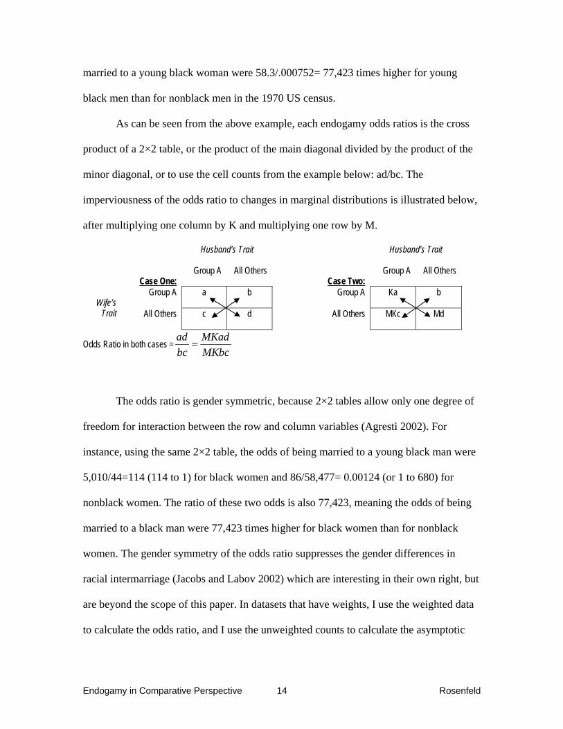
As can be seen from the above example, each endogamy odds ratios is the cross

product of a 2×2 table, or the product of the main diagonal divided by the product of the

minor diagonal, or to use the cell counts from the example below: ad/bc. The

imperviousness of the odds ratio to changes in marginal distributions is illustrated below,

after multiplying one column by K and multiplying one row by M.

Husband’s Trait

Husband’s Trait

Case One:

Group A All Others Case Two:

Group A All Others

Group A a b Group A Ka b Wife’s

Trait All Others c d

All Others MKc Md

Odds Ratio in both cases =ad MKadbc MKbc

=

The odds ratio is gender symmetric, because 2×2 tables allow only one degree of

freedom for interaction between the row and column variables (Agresti 2002). For

instance, using the same 2×2 table, the odds of being married to a young black man were

5,010/44=114 (114 to 1) for black women and 86/58,477= 0.00124 (or 1 to 680) for

nonblack women. The ratio of these two odds is also 77,423, meaning the odds of being

married to a black man were 77,423 times higher for black women than for nonblack

women. The gender symmetry of the odds ratio suppresses the gender differences in

racial intermarriage (Jacobs and Labov 2002) which are interesting in their own right, but

are beyond the scope of this paper. In datasets that have weights, I use the weighted data

to calculate the odds ratio, and I use the unweighted counts to calculate the asymptotic


standard error of the natural log of the odds ratio (Clogg and Eliason 1987), which in turn

is used to calculate the confidence intervals of the odds ratios.

Young blacks in Figure 1 have the highest odds ratios of endogamy across all

censuses, reaching a peak of more than one million in 1920. The endogamy odds ratios

for all major racial groups have declined fairly consistently over time. By the 2005 ACS,

the endogamy odds ratios for blacks had fallen to 715 (meaning that the odds of marrying

a black woman were still 715 times higher for black men than for non-black men). The

endogamy odds ratio for young Hispanics had fallen to 56 (in 2005) from 464 (in 1970).

The endogamy odds ratio for Asians fell from 94,000 (in 1950) to 199 (in 2005), and the

endogamy of young whites followed a similar downward path.

The picture for educational intermarriage is different in two respects. First,

educational endogamy has always been less powerful than racial endogamy in the U.S.,

meaning the odds ratios for educational endogamy have always been lower than the odds

ratios for racial endogamy. Secondly, whereas racial endogamy follows a pattern of steep

decline especially after 1960, educational endogamy has declined at a much more modest

rate. In 1940, the odds ratio for college degree endogamy was 34, and this declined to 23

in 1960, to 19 in 1970, and 17 by 2005. The odds ratio for some college endogamy was

21 in 1940, and this declined to 7.2 in 1990, before rising to 8.3 by 2005.5

One way to put the odds ratios of educational endogamy into perspective is to find

ethnic and ancestral groups whose odds ratios for endogamy have similar values. The

ancestral white ethnic groups “English,” “Irish,” “German,” and “Italian” each had odds

5 Although this finding of declining educational endogamy odds ratios runs against the grain of the dominant modernization hypothesis, the decline in educational endogamy as measured by simple odds ratios is fairly robust. The same pattern of steady decline is observed for expanded age categories. For ages 20-39, college degree endogamy declined from an odds ratio of 26 in 1940 to 12.6 in 2000. For all ages college degree endogamy there was a decline from odds ratio 23.9 in 1940 to 10.3 in 2000.


ratios for endogamy for US born persons in the neighborhood of 10 in the 1980-2000

period (not shown in Figure 1), with the English being slightly higher and the Germans,

Irish, and Italians having slightly lower rates of endogamy (Rosenfeld 2002, table 2). For

US natives, the identification with “English” or “Irish” identity is what Mary Waters

refers to as an “optional identity,” meaning it is an identity that individuals may choose to

express at times and in ways that are convenient to them (Waters 1990). This does not

imply that a college education (or Irish or German identity) are somehow unimportant in

the marriage market. The mate selection process is and always has been educationally

selective, but the strength of educational selectivity in the marriage market in the US has

always been modest compared to the powerful divisions of race.

Another way to put trends in educational endogamy into perspective is to compare

the trends in college degree endogamy and some college endogamy from the 1940-2000

with the trends for literacy endogamy in 1880-1930. Although literacy endogamy for

young US-born couples ended up at nearly the same level in 1930 (odds ratio of 47) as it

had been in 1880 (odds ratio of 42), there was a fairly powerful dip in literacy endogamy

to an odds ratio of 11 in 19106. Compared to the fluctuations in the odds ratio of literacy

endogamy, which ranged over a factor of 4 in 50 years, the raw odds ratios of college

degree endogamy declined by a factor of 2 in 60 years, a comparatively modest change.

Religious endogamy for Protestants and Catholics, like educational endogamy,

was at least an order of magnitude weaker (in odds ratio terms) than racial endogamy. In

the 1955 GAF survey, the odds ratios for Protestant and Catholic endogamy were 19.2

and 19.4, respectively.

6 In theory, literacy included the ability to read and write in any language, but the ability of the census enumerators to determine literacy in languages other than English may not have been very good.


Jewish endogamy was substantially higher than Catholic or Protestant endogamy,

with values between Asian and Hispanic endogamy, suggesting that the social barriers

between Jews and Christians are still relatively high, though declining. In the 1955 GAF,

Jewish endogamy had an odds ratio of 1483, declining to 580 in the late 1970s, 349 in the

1980s, and 197 in the 1990s (using data from the GSS). Because there were too few

young married Jews in the GSS and the GAF, I included respondents of all ages in the

calculations of Jewish endogamy which tends to overstate endogamy somewhat by

including couples married earlier (when social barriers against Jewish- Christian

intermarriage were higher). If Jewish endogamy were calculated using only respondents

from the middle Atlantic states (where most Jews in the US live), the odds ratios of

Jewish endogamy would be cut by about 50%, but Asians and Hispanics are also

geographically concentrated in the US (albeit in different areas), and the geographic

concentration of US born persons from all these groups is not accidental; rather it is part

of the considerable (but rapidly declining) social isolation of all three groups.

The odds ratios of endogamy for Catholics and Protestants were nearly identical

in 1955 because the Catholics and Protestants combined were more than 95% of the

population in the U.S. in 1955. The impact of the other (non-Catholic and non-Protestant)

groups was relatively small on the marriage choices of Catholics and Protestants and

therefore from the Catholic and Protestant perspectives, there were only two groups (if

we take the Protestants as an aggregate group). Since a 2×2 table yields only a single

degree of freedom for association, the odds ratios of Protestant and Catholic endogamy

were nearly the same. As the number of non-Christians and religiously nonaffiliated

persons has increased over time, Protestant and Catholic endogamy have diverged


slightly, so that in the early 1990s GSS sample, Protestant endogamy had an odds ratio of

4.2, and Catholic endogamy had an odds ratio of 5.5.

From the late 1970s to the early 1990s (the time frame over which the GSS

provides the religion both spouses were raised in), Protestant and Catholic endogamy

declined only slightly, and the differences were not statistically significant. In order to

see a significant decline in Protestant or Catholic endogamy, one has to compare the 1955

GAF to the GSS surveys from two decades later. To the extent that religious endogamy is

a sign of secularization at the level of the influence of traditional church organizations

over personal life (Chaves 1994), the secularization of Christians seems to predate 1970,

whereas the secularization of Jews is continuing. This is potentially significant because

most of the recent debate over secularization in the U.S. refers only to Christian

secularization and relies on data (such as the GSS) which were collected after 1970.

Although Kennedy described the US as a triple melting pot (with Jews,

Protestants, and Catholics as the three groups), and despite the fact that the doctrinal and

social divisions between Catholics and Protestants may have been bitterly contested in

the US in the distant past, none of the Christian subgroups have a strong enough odds

ratio of endogamy to be considered substantially isolated from other Christians in the US

any longer. Religious endogamy of the constituent Protestant groups in the 1977-1994

GSS was roughly the same (in odds ratio terms) as Protestant endogamy overall.

Mainline Protestant endogamy tended to be slightly lower, while Baptists and evangelical

Protestants had slightly higher levels of religious endogamy, but all the Protestant groups

had odds ratios of religious endogamy less than 10, indicating that intermarriage between

Protestant sects, and between Protestants and other Christians was fairly common.


Religious endogamy for the “no religious preference” or “decline to state” category was

very similar to Protestant and Catholic endogamy, with an odds ratio of 30 in 1955, and a

flat odds ratio of roughly 4 in the GSS in the 1970s, 1980s, and 1990s.

The growth over time in the nonaffiliated population of the US has raised many

questions about whether their growth is a sign of secularization (Chaves 1994; Hout and

Fischer 2002; Marwell and Demerath 2003). The fact that individuals who decline to

state any religious affiliation have marriage patterns so similar to the marriage patterns of

self-identified Protestants and Catholics is one sign that the nonaffiliated are not as

different from the self-identified Christians as some might suppose. It seems likely that

most of the religiously nonaffiliated have Christian ancestors and have a secular

familiarity with Christianity which allows them to mix easily with the majority Christian

population. In the context of religious endogamy, the unaffiliated behave as Christians.

Percentages of Racial, Educational, and Religious Endogamy

In order to put the raw odds ratios from Figure 1 into a different perspective,

Table 1 presents the simple percentages for endogamy, for women and men from the

same racial, educational, and religious groups as Figure 1, using the same data sources.

Table 1 shows that white and black and endogamy are by far the strongest types of

endogamy in percentage terms. Considering that whites have always comprised more

than 85% of the US population (ignoring Hispanicity), meaning that 85% of potential

mates were also white, the achievement of 99.6% endogamy for white women in 1970 is

less astonishing than the achievement of 99.1% endogamy for black women given that

only 10% of potential mates were black. The percentage endogamy for whites was


higher, but the odds ratio of endogamy (which takes group size into account) was higher

for blacks (see Figure 1).

[Table 1 here]

Several gender differences are highlighted by Table 1. First, black men have been

much less racially endogamous than black women, and the gap seems to have grown

wider since 1970 (Jacobs and Labov 2002). Second, the percentage of college degree

endogamy was much higher for women than for men in the mid 20th century, because

men with college degrees outnumbered women roughly two to one, so it was much more

difficult for men with college degrees to find wives who had the same level of education.

For young US born men with college degrees, the percentage who married women who

also had college degrees has been rising monotonically from 30% in 1940 to 74% in

2005, as women’s educational attainment has risen. The percentage of young US born

women with college degrees who married men who also had college degrees actually

declined, from 70.4% in 1970 to 62.6% in 2005. For a more detailed analysis of the

patterns of gender differences in educationally heterogamous unions, see Schwartz and

Mare (2005) and Schoen and Wooldredge (1989).

Racial Endogamy by Educational Attainment:

One central prediction of Milton Gordon’s classic (1964) treatise on assimilation

and intermarriage was that higher education would tear down some of the vestigial

barriers of race. More specifically, Gordon expected college educated people to marry


without regard to race, because race was an ascriptive marker which the highly educated

would presumably see beyond. Gordon’s prediction that higher education would erode

racial endogamy emerged directly from the bosom of modernization theory.

Table 2 presents the raw odds ratios of racial endogamy calculated with three

separate educational samples of 1980 census data, for whites, blacks, Asians and

Hispanics. The first sample contains only married couples whose spouses both had less

than a high school degree. The second sample includes only couples whose spouses both

had at least a high school degree, but less than a college degree. The third sample

includes only couples whose spouses both had at least a college degree. Since the odds

ratios control for the marginal distributions of both spouses by race, and since the

samples are educationally specific, these odds ratios of racial endogamy control for the

educational attainments of each racial group.

[Table 2 here]

Since age is associated with educational attainment, Table 2 relies on couples (of

any age) married for the first time within 10 years of the 1980 census rather than young

married couples (Rosenfeld 2005). Age at marriage is not available in the 1990 or 2000

U.S. censuses, so 1980 is the most recent census that can be used in this way. For U.S.

born persons with less than high school education married in the 1970s, the odds ratio of

black endogamy was 17,101. For young married couples with college degrees, the odds

ratio of black endogamy was 13,181. The odds ratio of black endogamy was smaller for

blacks with the highest level of education (a ratio of 0.77), but the ratio was not


significantly different from 1 (the confidence interval, 0.53-1.12, straddled 1). For white

endogamy the picture was similar: college degree couples had a slightly lower tendency

to racial endogamy, 0.88 times as high as high school dropout couples, but the ratio was

not significantly different from 1.

Asian Americans endogamy was half as high among the college educated (odds

ratio of 591) as among couples with less than high school degrees (odds ratio 1,160) and

the ratio was significantly different from 1. U.S. born Hispanics are the only group whose

pattern of ethnic or racial endogamy in the 1970s was dramatically altered by higher

education. The odds ratio of Hispanic endogamy was 479 for couples in the lowest

educational group, but only 71 for couples with college degrees, a ratio of roughly 7 to 1.

Since these odds ratios control for the size of the racial groups in each educational

category, the influence of education on Hispanic endogamy was not a simple matter of

the different educational profile of Hispanics relative to other groups. The comparatively

low level of endogamy for Hispanics with bachelors degrees indicates either that college

education eliminated most of the social barriers between Hispanics and non Hispanics, or

else that the U.S. born Hispanic population which has the opportunity to attend college

was very different from and much less socially isolated than the U.S. born Hispanic

population which did not attend college.

Table 2 helps put the unique power of race into perspective. Among married

people with college degrees in 1980 the odds ratios of black, white and Asian endogamy

were more than 10 times higher (and for blacks, more than 100 times higher) than the

odds ratios of educational endogamy in the general U.S. population. Race (Hispanicity

excepted), even for the highly educated, was a far stronger divide in the marriage market


than education or than the division between Protestants and Catholics. Table 2 also helps

put Gordon’s theory of educational effects on racial endogamy into perspective. Except

for Hispanics, the effects of education on racial endogamy were not very strong for

people married in the 1970s.

The relatively high power of racial endogamy, even at the end of the 20th century,

means that well more than 90% of all marriages in the U.S. continue to be racially

endogamous. In a separate appendix available from the author, I show (using a variety of

loglinear models) that the overall impact of the interaction between race (for blacks and

whites) and education in the U.S. marriage market is relatively minor. The fact that the

odds ratios of racial endogamy are not much affected by compositional changes in

education (and vice-versa) helps justify the comparison of raw odds ratios in Figure One,

as a first order estimate of each group’s closure in the marriage market.

Protestant Endogamy in Historical Perspective:

In order to put the changes in the raw odds ratios of religious endogamy into

broader historical perspective, Figure 2 includes odds ratios for Protestant endogamy

calculated from Kennedy’s (1952) table 2 as well as odds ratios calculated from the 1955

GAF, the 1977-1994 GSS, and the 1965 NFS. In Kennedy’s data, the Protestant and

Catholic endogamy odds ratios cannot be distinguished for methodological reasons,

whereas in the other datasets Catholic and Protestant endogamy have been nearly the

same, so for simplicity here I limit the discussion to Protestant endogamy.


[Figure 2 here]

Kennedy’s data have many limitations. First of all, Kennedy only reported row

percentages and overall sample size. We know her sample included 920 marriage licenses

from 1870, 1,770 licenses from 1900, 2,538 licenses from 1930 and 3,816 licenses from

1940 (Kennedy 1944 p.331), but we don’t know how many of the marriage licenses were

for Protestant brides. Second, Kennedy only had access to the religion reported on

marriage licenses; premarital conversion would tend to make marriage license records

appear more religiously endogamous. Third, the New Haven marriage licenses may have

only recorded the religion of one spouse. Kennedy seems to have used one spouse’s

national origin as a proxy for religion, assuming for instance that all Germans in New

Haven were Protestants, and that all Irish were Catholics. These three flaws make

Kennedy’s data suspect, but the uniquely long time span of Kennedy’s religious

endogamy data make the data potentially useful despite their limitations.

I calculated a single odds ratio for Protestant endogamy from each year of

Kennedy’s (1952 p.57) Table 2 by excluding the Jews (whose number was unknown but

certainly small) and using the endogamy percentages for Catholics and Protestants as the

entries in a 2×2 table from which the odds ratio is the simple cross product. Since the

odds ratio is immune to changes of scale, the odds ratio based on percentage entries is the

same as the odds ratio one would obtain from the raw number of marriages in each cell of

the table. For instance in 1870, 99.11% of Protestants married other Protestants, and

95.35% of Catholics married other Catholics, so the odds ratio would be:

.9911(.9535) 2,283.5

.0089(.0465)= .


Unfortunately, without the raw number of marriages in each cell, the confidence interval

for the odds ratio is unknown.

The Protestant endogamy odds ratios of 17 for 1930, 30.8 for 1940, and 6.5 for

1950 derived from Kennedy’s sample of New Haven marriages are within the confidence

intervals of most of the other local and national sources for Protestant endogamy for

marriages recorded in those decades. Burgess and Wallin’s 1937-39 sample of young

white couples in Chicago had a Protestant endogamy odds ratio of 41 with a 95%

confidence interval of 28-61 (not shown in Figure 2). According to GSS data on first

marriages,7 Protestant endogamy had an odds ratio of 15.8 (confidence interval 12-21) in

the 1930s, 12.3 (confidence interval 10-15) in the 1940s, and 9.4 (confidence interval 8-

11) in the 1950s

Figure 2 shows that the odds ratios for Protestant endogamy derived from

Kennedy’s New Haven data is roughly consistent with GSS, NFS, and GAF data for

Protestant endogamy for marriages celebrated in the 1930s, 1940s, and 1950s. The

consistency of Kennedy’s New Haven data with the national data on Protestant

endogamy for marriages celebrated in the mid 20th century suggests that, despite their

flaws, Kennedy’s local data on religious endogamy are not a bad estimate for national

trends.

The odds ratio of religious endogamy derived from Kennedy’s 1870 sample is

especially interesting because at 2,283.5 it is 33 times larger than the odds ratio of 68.5

derived from her 1900 data. Is it possible that the 1870 figure is completely misleading?

7 The GSS data used here include age at first marriage, with no indication of whether the current marriage is the respondent’s first marriage (age at current marriage was only available from the 1994 GSS, and sample size was insufficient). The GSS figures for Protestant endogamy are less than the GAF and NFS because some of the GSS couples were second and third marriages celebrated more recently, when religious endogamy in the US was lower.


Kennedy’s data had 920 marriage licenses from 1870. Protestants were certainly in the

majority in New Haven in 1870, but there should have been enough Catholics in the

marriage record sample from New Haven in 1870 to allow for a reasonable confidence

interval around the endogamy odds ratio. Irish Catholics had been immigrating to the

eastern U.S. since the early 1800s, with a peak during the Potato famines of the 1840s

(Ignatiev 1995). If Kennedy’s religious endogamy data series is to be believed, then the

implication is that social barriers between Protestants and Catholics in New Haven

declined dramatically between 1870 and 1900.

A Graphical Representation of the Saturated Model for Educational Assortative

Mating:

The raw odds ratios of educational endogamy I presented in Figure One were

simple to calculate and easy to interpret, but the raw odds ratios overlook much of the

complex pattern of educational assortative mating. Years of formal education constitutes

an ordinal scale, which implies that the pattern of off-diagonal interactions is worthy of

careful attention. In order to understand the pattern of educational assortative mating, one

needs to understand not only how often spouses have the same education, but how often

spouses’ educational attainments differ by one category, or two categories, and so on

(Mare 1991; Schwartz and Mare 2005). My approach to the complex picture of

educational assortative mating is different from the approach that has usually been taken

in the published literature. Rather than fitting loglinear models to the data and then trying

to make sense out of a subset of coefficients from a few of the models, I use the saturated


model of husband’s education by wife’s education to fit the data exactly (Goodman

1970). I then plot the full set of interaction terms so that the entire pattern of interactions

can be examined graphically and compared across census years.

My approach here has both advantages and disadvantages when compared to the

usual loglinear modeling approach. One advantage of using saturated models is that the

data presented are the actual data, not the fitted data which may come closer to the actual

data in some places than in others. Since the usual fit statistics for loglinear models (the

likelihood ratio test, the BIC, the AIC) are global fit statistics, the question of how the

model fits in the theoretically most important cells is usually left unanswered (Rosenfeld

2005; Weakliem 1999). One could supplement the usual loglinear model fitting approach

with a detailed study of the standardized residuals for all cells across models, but this is

rarely done.

When graphing data, Tufte (2001 p.95) cautions against graphing predicted values

or smoothed data in lieu of the observed data. Graphing interaction coefficients from the

saturated model satisfies Tufte’s criteria for data presentation because while the

interaction coefficients represent a transformation of the observed data, the saturated

model fits the data exactly without simplifying or smoothing.

Since the saturated model has one term for every cell in the cross tabulated

dataset, the saturated model is the least parsimonious of all possible models. The

saturated model’s lack of parsimony is certainly a liability if one seeks the simplest and

most parsimonious description of the data (Agresti 2002; Bishop, Fienberg and Holland

1975). As the number of interactions in a loglinear model grows, however, the

interpretation of the interaction coefficients becomes much more difficult, and the


analytical advantages of parsimony dissipate. A complex loglinear model can, because of

the difficulty of interpreting the coefficients, obscure the data as easily as it can simplify

or clarify the data (Rosenfeld 2005). Finally, the saturated model demands a nonzero (and

preferably substantial) number of counts in every cell, a requirement which in the case of

census data is not difficult to satisfy.

The dataset includes couples whose spouses were both age 20 to 39 and both U.S.

born from the 1940, 1960, 1980 and 2000 censuses. I use 20 year spans between

censuses, and I use age groups 20 years wide in order to minimize the problem of shifting

age at marriage and increasing educational participation by young adults in their 20s

(Rosenfeld 2005). The education categories were compressed to 5 in order to decrease

sparseness from the data and in order to decrease clutter in the figures: less than 9th

grade, 9th-11th grade, high school degree, some college, and bachelor’s degree or more.

The dataset of 5×5×4=100 cells has 1,704,309 cases (unweighted), and the smallest cell

has 120 (unweighted) couples.

Within each census year’s data, the loglinear model takes the saturated form

Log(U)=HusbEd×WifeEd

where U are the predicted (and actual) counts. The coefficients for HusbEd and WifeEd

sum to zero, and the educational interaction terms also sum to zero, and the lower order

terms are implied. Having the coefficients sum to zero ensures that the coefficients will

be the same regardless of which educational category is the comparison category. The


coefficients are then exponentiated make them more comparable with the simple odds

ratios discussed earlier in the paper, and plotted on a log scale.8

[Figure 3 here]

Figure 3 is composed of four figures: the educational interactions for 1940, 1960,

1980, and 2000. The figures describe the pattern of educational assortative mating purged

of any effects of changing educational distributions over time. The figures include all 25

educational interactions even though only 16 of the interactions can be mutually

independent. The figures include all interactions whether they were statistically

significant or not. An alternative set of figures which includes the changes in educational

endogamy over time is available from the author.

The pattern of educational assortative mating is quite stable from 1940 to 2000;

each figure takes a ‘saddle’ shape. The educational endogamy diagonal points toward the

reader’s right shoulder. The adjusted odds ratios are highest along the endogamy

diagonal, with peaks in educational endogamy at the highest and lowest educational

levels, meaning the highest and lowest educational groups were the most isolated in the

marriage market. The adjusted odds ratios fall with each step away from the endogamy

diagonal, meaning that the likelihood of intermarriage declines as the difference between

8 The models account for census weights in the manner described by Clogg and Eliason (1987). For sum to zero parameter constraints, see Hout (1983 p.20) or Agresti (2002 p.317). The values plotted in Figure 3 are exponentiated coefficients from the saturated loglinear model described above. The saturated loglinear model coefficients can be produced by direct calculation from the tables of marriage counts by husbands’ and wives’ educations, without recourse to specialized software. First take the natural log of each cell count. Then subtract the each census year’s mean log count from each cell, and then subtract the mean of each row and of each column from their respective rows and columns. What remains in each cell are the interaction coefficients from a saturated loglinear model, or the log counts purged of row and column effects, with global, row, and column means of zero. The “sums to zero” coding constraint becomes a “product of one” constraint after the values are exponentiated.


spouses’ educational attainments increases. The saddle pattern is the typical pattern for

educational assortative mating. The four census years covered in Figure 3 are all plotted

on the same scale, which illustrates that not only the shape but also the magnitude of the

intensity of educational assortative mating has remained roughly consistent from 1940 to

2000, though Figure 3 does also show growth along the endogamy diagonal which is

consistent with modernization theory.

Educational endogamy for individuals with college degrees increased across the

four censuses, from an adjusted odds ratio of 7.7 in 1940 to an adjusted odds ratio of 15.5

in 2000, and the differences were statistically significant. The finding of increasing

educational endogamy for persons with college degrees (after accounting for all other

changes in educational assortative mating) in Figure 3 contrasts with the raw odds ratios

in Figure One, which showed a decline of college degree endogamy from 34.3 in 1940 to

17.1 in 2000.

The fact that Figure 3 accounts for all other changes in educational assortative

mating is the reason Figure 3 seems to show increasing educational endogamy over time

while Figure 1 shows the reverse. Examining only the educational endogamy terms in

Figure 3 (the main diagonal) while ignoring the off-diagonal interactions is, however, an

exercise in selective analysis. The off-diagonal cells in Figure 3 hide changes, some of

which are contrary to the predictions of modernization theory, which influence the main

diagonal because all interactions are estimated jointly. In a loglinear model which

includes only the main diagonal (i.e. only the educational endogamy terms, results

available from the author), the odds ratio of educational endogamy for persons with

college degrees actually declines across all 4 censuses, while the educational endogamy


of those in the lowest educational category increases across the four censuses. The

empirical contradictions are not easily resolved. Single statistic measure of the correlation

between wives’ and husbands’ educations (gamma, Cramer’s V, tau-b, available from the

author) generally show slight declines over time, consistent with Figure 1. Where do

these contradictory findings with regard to educational endogamy leave us? If the results

with regard to educational endogamy over time depend on relatively arbitrary choices of

modeling strategy, perhaps it is time to acknowledge that the trend in educational

endogamy is not as clearly positive as is commonly supposed.

Discussion:

Although this paper has focused on broad descriptive comparisons rather than on

detailed hypothesis testing, the data do suggest several conclusions which confirm prior

findings, and several other conclusions which suggest that some prior assumptions need

to be re-examined.

The decline of racial endogamy has been widely reported. What has not always

emerged so clearly from the literature on racial intermarriage is the extent to which racial

barriers are still, even after decades of decline, dramatically more powerful than any

other kind of social barriers in the marriage market. Some of the understatement of the

importance of race is due to the way the early pioneers in intermarriage research either

overlooked race (Kennedy 1944; Kennedy 1952) or assumed (incorrectly, it turns out)


that racial divisions would be mitigated or overcome through social status or higher

education (Gordon 1964).

The story of religious endogamy in the U.S. is an incomplete story for the simple

reason that the data are inadequate. The best data most often used to study religious

attitudes in the U.S. (the GSS) do not extend far enough back in time to capture

secularization when it may have been a much more powerful force. In the late 20th

century US, the mainline Protestants, evangelical Protestants, Catholics, and even those

who declined to state any religious affiliation all had low odds ratios of endogamy which

suggest that these groups mixed relatively freely with each other. Kennedy’s triple

melting pot was an appropriate description of New Haven in 1870, but was no longer an

apt description of New Haven by 1944 when she published her first article on the subject.

Only the Jews continue to be highly isolated from other religious groups in the US

marriage market, and the marriage market isolation of the Jews has declined sharply in

recent years. The increasing intermarriage of Jews with non-Jews is a source of concern

for some in the Jewish community who see outmarriage and assimilation as eventually

eroding the size of the Jewish population in the US (Mayer 1985; Phillips 1996; Phillips

2005). The marriage market isolation of Buddhists, Muslims, and other non-Christian

groups in the US cannot be reliably determined from the currently available data.

Although modernization theory with its prediction of increasing educational

endogamy has dominated the literature on educational assortative mating in recent years

(Kalmijn 1991a; Mare 1991; Schwartz and Mare 2005), the literature and the data both

offer room for divergent interpretations (Blau and Duncan 1967; Liu and Lu 2006; Smits,

Ultee and Lammers 1998). In my view the diversity of claims about educational


assortative mating results not only from the inherent difficulties in studying a

complicated system, but also from the subtlety of the actual changes over time. Even

subtle changes in educational assortative mating can have important societal impacts, so

whether one views the actual changes as profound or as minor is a matter of perspective.

If one compares the changes in educational assortative mating to the radical changes in

racial endogamy over the same period (as I do in this paper), the educational assortative

mating system appears to have been remarkably stable.

One of the reasons hypothesized for the decline of racial endogamy is that young

adults are marrying later, and have a greater opportunity to travel and to meet potential

mates beyond the watchful eyes of their parents and outside of the boundaries of the

highly racially segregated neighborhoods of their youth (Rosenfeld and Kim 2005). The

post-1960 independence of young adults would not be expected to have much of an effect

on educational endogamy, for several reasons. First, residential neighborhoods are not

nearly as segregated by education (parental education or children’s education) as they are

segregated by race (Massey and Denton 1993; White 1987). Even in the past when young

adults found most of their mates in the neighborhood (Bossard 1932; Kennedy 1943), the

set of potential mates would not have been educationally homogeneous. Second,

educational intermarriages have never been strongly socially stigmatized in the US.

Whereas racial intermarriage used to be illegal in much of the US, and whereas many

religious denominations have a tradition (only recently eroded) of refusing to recognize

religious intermarriage, there have never been any ardent institutional opponents of

educational intermarriage.


Modernization theory’s claim that educational endogamy has increased over time

has fueled the argument that the cognitive elite in the US are becoming increasingly

isolated from the rest of American society (Herrnstein and Murray 1994 p.110-112, 509-

526). Herrnstein and Murray’s claim of increasing cognitive stratification in the US rests

on several shaky premises. First, as I have tried to show in this article, the trend in

educational endogamy over time is not as clear as is sometimes supposed. Second, Mare

(2000) has argued that even a high rate of increasing educational endogamy would not

affect societal stratification very much.

One of the reasons that the modernization theory of increasing educational

endogamy in the US is so popular is that it is difficult to imagine how wives’ educational

levels could have mattered as much 50 or 100 years ago, when few married women

worked. In order to understand the apparent paradox of relatively flat educational

endogamy during a period of rapidly increasing returns to education in the labor market,

one must remember that spousal choice is a social and personal decision that goes far

beyond income maximization.9 Educational endogamy has always existed, even when

women did not work, because social life (and therefore access to potential mates) is and

always has been heavily stratified by class (Kalmijn 1998). Social homophily, or the

preference for the company of those with tastes and preferences and backgrounds similar

to one’s own, is also a vital element in mate selection (Bourdieu 1984; Kalmijn 1998;

Rosenfeld 2005). Unlike returns to education in the labor market, the non-economic

causes of educational endogamy have probably been fairly stable over time.

9 Even in the realm of income, the first assumptions about how women’s labor force participation might increase the income inequality between families have not been substantiated by the data (Cancian and Reed 1999; Danziger 1980). The income inequality of families has risen at roughly the same rate as the income inequality of individuals, in part because most of the increase in income inequality is driven by inequality in men’s earnings (Levy and Murnane 1992).


References

Agresti, Alan. 2002. Categorical Data Analysis. Second Edition. Hoboken, New Jersey: Wiley Interscience.

Berger, Peter L. 1969. A Rumor of Angels: Modern Society and the Rediscovery of the Supernatural. Garden City: Doubleday & Company.

Bishop, Yvonne M, Stephen E. Fienberg, and Paul Holland. 1975. Discrete Multivariate Analysis: Theory and Practice. Cambridge, Mass.: MIT Press.

Blackwell, Debra L. 1998. "Marital Homogamy in the United States: The Influence of Individual and Paternal Education." Social Science Research 27:159-188.

Blau, Peter M, and Otis Dudley Duncan. 1967. The American Occupational Structure. New York: The Free Press.

Blau, Peter M., and Joseph E. Schwartz. 1984. Crosscutting Social Circles: Testing a Macrostructural Theory of Intergroup Relations. Orlando, FL: Academic Press.

Bossard, James H. S. 1932. "Residential Propinquity as a Factor in Marriage Selection." American Journal of Sociology 38:219-224.

Bourdieu, Pierre. 1984. Distinction: A Social Critique of the Judgment of Taste. Translated by Richard Nice. Cambridge, Mass.: Harvard University Press.

Burgess, Ernest W., and Paul Wallin. 1943. "Homogamy in Social Characteristics." American Journal of Sociology 49:109-124.

Cancian, Maria, and Deborah Reed. 1999. "The Impact of Wives' Earnings on Income Inequality: Issues and Estimates." Demography 36:173-184.

Chaves, Mark. 1994. "Secularization as Declining Religious Authority." Social Forces 72:749-774.

Clogg, Clifford C., and Scott R. Eliason. 1987. "Some Common Problems in Log-Linear Analysis." Sociological Methods and Research 16:8-44.

Clogg, Clifford C., and Edward S. Shihadeh. 1994. Statistical Models for Ordinal Variables. Thousand Oaks, Calif.: Sage Press.

Danziger, Sheldon. 1980. "Do Working Wives Increase Family Income Inequality." Journal of Human Resources 15:444-451.

Goldstein, Sidney. 1969. "Socioeconomic Differentials Among Religious Groups in the United States." American Journal of Sociology 74:612-631.

Goodman, Leo A. 1970. "The Multivariate Analysis of Qualitative Data: Interactions among Multiple Classifications." Journal of the American Statistical Association 65:226-256.

Gordon, Milton. 1964. Assimilation in American Life: The Role of Race, Religion, and National Origin. New York: Oxford University Press.

Gorski, Philip S. 2000. "Historicizing the Secularization Debate: Church, Sate, and Society in Late Medieval and Early Modern Europe, CA. 1300 to 1700." American Sociological Review 65.

Greeley, Andrew M. 1972. Unsecular Man: The Persistence of Religion. New York: Schocken Books.


Hallinan, Maureen T., and Richard A. Williams. 1989. "Interracial Friendship Choices in Secondary Schools." American Sociological Review 54:67-78.

Herrnstein, Richard J., and Charles Murray. 1994. The Bell Curve: Intelligence and Class Structure in American Life. New York: The Free Press.

Hout, Michael. 1983. Mobility Tables. Newberry Park, Calif.: Sage. Hout, Michael, and Claude Fischer. 2002. "Why More Americans Have No Religious

Preference: Politics and Generations." American Sociological Review 67:165-190. Ignatiev, Noel. 1995. How the Irish Became White. New York: Routledge. Jackman, Mary R. 1978. "General and Applied Tolerance: Does Education Increase

Commitment to Racial Integration?" American Journal of Political Science 22:302-324.

Jacobs, Jerry A., and Teresa G. Labov. 2002. "Gender Differentials in Intermarriage Among Sixteen Race and Ethnic Groups." Sociological Forum 17:621-646.

Johnson, Robert Alan. 1980. Religious Assortative Marriage in the United States. New York: Academic Press.

Kalmijn, Matthijs. 1991a. "Shifting Boundaries: Trends in Religious and Educational Homogamy." American Sociological Review 96:786-800.

—. 1991b. "Status Homogamy in the United States." American Journal of Sociology 97:496-523.

—. 1998. "Intermarriage and Homogamy: Causes, Patterns, Trends." Annual Review of Sociology 24:395-421.

Kennedy, Ruby Jo Reeves. 1943. "Premarital Residential Propinquity and Ethnic Endogamy." American Journal of Sociology 48:580-584.

—. 1944. "Single or Triple Melting Pot? Intermarriage Trends in New Haven, 1870-1940." American Journal of Sociology 49:331-339.

—. 1952. "Single or Triple Melting Pot? Intermarriage in New Haven, 1870-1950." American Journal of Sociology 58:56-59.

Kreider, Rose Marie. 1999. Interracial Marriage and Marital Instability. Ph.D. Thesis, Sociology, University of Maryland.

Levy, Frank, and Richard J. Murnane. 1992. "U.S. Earnings Levels and Earnings Inequality: A Review of Recent Trends and Proposed Explanations." Journal of Economic Literature 30:1333-1381.

Lieberson, Stanley, and Mary C. Waters. 1988. From Many Strands: Ethnic and Racial Groups in Contemporary America. New York: Russell Sage Foundation.

Liu, Haoming, and Jingfeng Lu. 2006. "Measuring the Degree of Assortative Mating." Economics Letters 92:317-322.

Mare, Robert D. 1991. "Five Decades of Educational Assortative Mating." American Sociological Review 56:15-32.

—. 2000. "Assortative Mating, Intergenerational Mobility, and Educational Inequality." California Center for Population Research working paper CCPR-004-00. http://www.ccpr.ucla.edu/.

Marwell, Gerald, and N. J. Demerath, III. 2003. "'Secularization' by Any Other Name." American Sociological Review 68:314-316.

Massey, Douglas S., and Nancy A. Denton. 1993. American Apartheid: Segregation and the Making of the Underclass. Cambridge, Mass.: Harvard University Press.


Mayer, Egon. 1985. Love and Tradition: Marriage Between Jews and Christians. New York: Plenum Press.

McPherson, Miller, Lynn Smith-Lovin, and James M. Cook. 2001. "Birds of a Feather: Homophily in Social Networks." Annual Review of Sociology 27:415-444.

Michielutte, Robert. 1972. "Trends in Educational Homogamy." Sociology of Education 45:288-302.

Moran, Rachel. 2001. Interracial Intimacy: The Regulation of Race and Romance. Chicago: University of Chicago Press.

Pencavel, John. 1998. "Assortative Mating by Schooling and the Work Behavior of Wives and Husbands." American Economic Review 88:326-329.

Phillips, Bruce A. 1996. "Re-Examining Intermarriage." Wilstein Institute of Jewish Policy Studies. http://hebrewcollege.edu/html/affiliates/wilstein_institute.htm.

—. 2005. "Assimilation, Transformation, and the Long Range Impact of Intermarriage." Contemporary Jewry 25:50-85.

Qian, Zhenchao. 1997. "Breaking the Racial Barriers: Variations in Interracial Marriage between 1980 and 1990." Demography 34:263-276.

—. 1998. "Changes in Assortative Mating: The Impact of Age and Education 1970-1990." Demography 35:279-292.

Qian, Zhenchao, and Daniel T. Lichter. 2007. "Social Boundaries and Marital Assimilation: Interpreting Trends in Racial and Ethnic Intermarriage." American Sociological Review 72:68-94.

Qian, Zhenchao, and Samuel H. Preston. 1993. "Changes in American Marriage 1972 to 1987: Availability and Forces of Attraction by Age and Education." American Sociological Review 58:482-495.

Quillian, Lincoln, and Mary E. Campbell. 2003. "Beyond Black and White: The present and Future of Multiracial Friendship Segregation." American Sociological Review 68:540-566.

Rockwell, Richard C. 1976. "Historical Trends and Variation in Educational Homogamy." Journal of Marriage and the Family 38:83-95.

Rosenfeld, Michael J. 2002. "Measures of Assimilation in the Marriage Market: Mexican Americans 1970-1990." Journal of Marriage and the Family 64:152-162.

—. 2005. "A Critique of Exchange Theory in Mate Selection." American Journal of Sociology 110:1284-1325.

Rosenfeld, Michael J., and Byung-Soo Kim. 2005. "The Independence of Young Adults and the Rise of Interracial and Same-Sex Unions." American Sociological Review 70:541-562.

Ruggles, Steven, Matthew Sobek, Trent Alexander, Catherine A. Fitch, Ronald Goeken, Patricia Kelly Hall, Miriam King, and Chad Ronnander. 2004. "Integrated Public Use Microdata Series: Version 3.0." Minneapolis, Minn.: University of Minnesota. www.ipums.org.

Ryder, Norman B., and Charles F. Westoff. 1965. "National Fertility Study 1965." Madison, Wisconsin: Center for Demography and Ecology.

Schoen, Robert, and John Wooldredge. 1989. "Marriage Choices in North Carolina and Virginia 1969-71 and 1979-81." Journal of Marriage and the Family 51:465-481.


Schuman, Howard, Charlotte Steeh, Lawrence Bobo, and Maria Krysan. 1997. Racial Attitudes in America: Trends and Interpretations. Revised Edition. Cambridge, Mass.: Harvard University Press.

Schwartz, Christine R., and Robert D. Mare. 2005. "Trends in Educational Assortative Marriage From 1940 to 2003." Demography 42:621-646.

Sears, David O. 1988. "Symbolic Racism." in Eliminating Racism, Profiles in Controversy, edited by Phyllis A. Katz and Dalmas A. Taylor. New York: Plenum Press.

Smits, Jeroen. 2003. "Social Closure Among the Higher Educated: Trends in Educational Homogamy in 55 Countries." Social Science Research 32:251-277.

Smits, Jeroen, Wout Ultee, and Jan Lammers. 1998. "Educational Homogamy in 65 Countries: An Explanation of Differences in Openness Using Country-Level Explanatory Variables." American Sociological Review 63:264-285.

—. 2000. "More or Less Educational Homogamy? A Test of Different Versions of Modernization Theory Using Cross-Temporal Evidence for 60 Countries: A Reply to Raymo and Xie." American Sociological Review 65:781-788.

Tufte, Edward R. 2001. The Visual Display of Quantitative Information. Second Edition. Cheshire, Conn.: Graphics Press.

U.S. Bureau of the Census. 1958. "Religion Reported by the Civilian Population of the United States: March 1957." Current Population Reports, P-20 79. Washington, D.C.

Wallenstein, Peter. 2002. Tell the Court I Love My Wife: Race, Marriage and Law- An American History. New York: Palgrave Macmillan.

Waters, Mary C. 1990. Ethnic Options: Choosing Identities in America. Berkeley, Calif.: University of California Press.

Weakliem, David L. 1999. "A Critique of the Bayesian Information Criterion for Model Selection." Sociological Methods and Research 27:359-397.

White, Michael. 1987. American Neighborhoods and Residential Differentiation. New York: Russell Sage.

Wilson, Bryan. 1976. Contemporary Transformations of Religion. London: Oxford University Press.


Table 1: Percentage Endogamy by Race, Education, and Religion for US born men and women

Women

1940 1950 1960 1970 1980 1990 2000 2005 white endogamy 99.9 99.9 99.9 99.6 99.0 98.7 96.2 96.0 black endogamy 99.2 99.4 99.5 99.1 98.7 96.8 94.1 90.2 Hispanic endogamy 77.6 68.7 63.2 66.6 61.1 Asian endogamy 81.3 89.4 76.2 59.6 45.6 41.3 32.9 41.6

some college endogamy 60.0 72.7 76.3 73.5 72.0 74.9 73.1 college degree

endogamy 56.2 69.3 70.4 66.7 63.7 61.8 62.6

1955 1970s 1980s 1990s Protestant endogamy 87.8 81.2 76.1 74.7 Catholic endogamy 67.0 53.6 54.3 53.8 Jewish endogamy 84 78† 70 62† no religious preference

endogamy 39 13† 20 22 Men 1940 1950 1960 1970 1980 1990 2000 2005 white endogamy 99.9 99.9 99.8 99.7 99.2 99.0 97.0 96.6 black endogamy 99.1 99.1 99.4 98.3 95.5 92.0 83.8 82.3 Hispanic endogamy 76.5 67.1 64.1 66.4 64.8 Asian endogamy 92.0 83.8 67.9 52.1 47.0 40.3 48.2 some college endogamy 47.7 49.9 59.0 64.5 75.3 81.7 85.4 college degree

endogamy 30.0 33.0 44.0 50.3 59.9 67.2 73.8

1955 1970s 1980s 1990s Protestant endogamy 87.0 80.7 77.8 74.3 Catholic endogamy 74.6 56.7 57,1 56.1 Jewish endogamy 87.5 66† 69 57† no religious preference

endogamy 11 9† 12 17†

Sources same as for Figure 1. For educational, racial and ancestral endogamy: Weighted census microdata and weighted data from the ACS 2005, both partners U.S. born and age 20-29. Source for religious endogamy: the General Social Survey,1978-1994, and the 1955 Growth of American Family survey. For Protestant and Catholic endogamy, respondents were US born and age 20-29. For the smaller samples of Jewish endogamy and no religious preference endogamy, respondents were US born all ages. Black and White categories include Hispanics for consistency with pre-1970 data. † N<50


Table 2: Odds Ratios of Racial Endogamy (with 95% confidence intervals) by Educational Attainment Educational Attainment of Both Spouses:

A: less than 12 years B: 12-15 years

C: 16 years or more

Odds Ratio High education

compared to low= C/A

Black Endogamy 17,101 17,241 13,181 0.77 (13,106- 22,314) (15,245- 19,498) (10,158- 17,103) (0.53- 1.12) White Endogamy 1,098 1,190 971 0.88 (970- 1,243) (1,124- 1,260) (854- 1,104) (0.74- 1.06) Asian Endogamy 1,160 590 591 0.51 (710- 1,895) (513- 678) (479- 729) (0.30- 0.87) Hispanic Endogamy 479 116 71 0.15 (425- 540) (110- 122) (61- 84) (0.12- 0.18) Source: weighted 1980 census 5% files via IPUMS. All couples consist of US born spouses, married in the 1970s, at least one spouse married for the first time. Black and white includes Hispanics.


Figure 1: Odds Ratios of Endogamy by Race, Education, and Religion, 1880-2005

1

10

100

1,000

10,000

100,000

1,000,000

10,000,000

1880 1890 1900 1910 1920 1930 1940 1950 1960 1970 1980 1990 2000

Odd

s R

atio

for E

ndog

amy

Black Endogamy

White Endogamy

Asian Endogamy

Jewish Endogamy

Hispanic Endogamy

Literate Endogamy

College degree endogamy

Some college endogamy

Catholic Endogamy

Protestant Endogamy

No religious preferenceendogamy

Larger endogamy odds ratios imply greater isolation in the marriage market. Source for educational, racial and ancestral endogamy: Weighted census microdata 1880-2000, and American Community Survey 2005, both partners U.S. born and age 20-29. Source for religious endogamy: the General Social Survey,1978-1994, and the 1955 Growth of American Family survey. For Protestant and Catholic endogamy, respondents were US born and age 20-29. For the smaller samples of Jewish endogamy and no religious preference endogamy, respondents were US born all ages. Black and White categories include Hispanics for consistency with pre-1970 data..


Figure 2: Protestant Endogamy Odds Ratios, Local and National Sources

1

10

100

1000

10000

1860 1880 1900 1920 1940 1960 1980 2000Year married

Year married, GAF, religionbefore marriage

Year married, NFS, currentreligion and religion of parents

Year first married, GSS,religion at age 16

Year married, New Haven, fromKennedy, religion at date ofmarriage

Sources: *1955 Growth of American Family Survey, year of current marriage and religion before marriage *1965 National Fertility Study, year of current marriage. Protestants are those whose religion in 1965 was Protestant and whose parents' religions were also Protestant. *General Social Survey data, year of first marriage (marriage number of respondent unknown), and religion at age 16. *New Haven endogamy from Kennedy’s (1952) study of marriage licenses, year of marriage license and religion reported on the license.


Figure 3: Consistency in the Pattern of Educational Assortative Mating for Young Couples Over Time

Source: Weighted census 1% files from 1940 and 1960, and 5% files from 1980, and 2000 censuses, via IPUMS. Individuals were all U.S. born and age 20-39 at the time of the census. The plotted values are exponentiated coefficients (or corrected odds ratios) from saturated loglinear models of husbands’ by wives’ education.

<9

9 to

11

HS

Som

e C

ol

BA+

<99

to 1

1H

SSo

me

Col

BA+

0.1

1

10

100

Wife Ed Husb Ed

1940

<9

9 to

11

HS

Som

e C

ol

BA+

<99

to 1

1H

SSo

me

Col

BA+

0.1

1

10

100

Wife Ed Husb Ed

1960

<9

9 to

11

HS

Som

e C

ol

BA+

<99

to 1

1H

SSo

me

Col

BA+

0.1

1

10

100

Wife Ed Husb Ed

1980

<9

9 to

11

HS

Som

e C

ol

BA+

<99

to 1

1H

SSo

me

Col

BA+

0.1

1

10

100

Wife Ed Husb Ed

2000

racial, educational, and religious endogamy in the united states

Documents