Racial Disparities in Job Finding and Offered Wages∗

Roland G. Fryer, Jr.

Harvard University

and NBER

Devah Pager

Princeton University

Jörg L. Spenkuch

University of Chicago

September 2011

Abstract

The extent to which discrimination can explain racial wage gaps is one of the most divisive

subjects in the social sciences. Using a newly available dataset, this paper develops a simple

empirical test which, under plausible conditions, provides a lower bound on the extent of discrim-

ination in the labor market. Taken at face value, our estimates imply that differential treatment

accounts for at least one third of the black-white wage gap. We argue that the patterns in our

data are consistent with a search-matching model in which employers statistically discriminate

on the basis of race when hiring unemployed workers, but learn about their marginal product

over time. However, we cannot rule out other forms of discrimination.

∗We give special thanks to Alan Krueger for access to the New Jersey data used in this paper. We also thank JosephAltonji, David Card, Kerwin Charles, William Hubbard, Lawrence Katz, Kevin Lang, Steven Levitt, Julie Mortimer,

Derek Neal, Ariel Pakes, and Betsey Stevenson as well as seminar participants at the University of Chicago and NBER

for helpful comments and discussions. We are also grateful to Joseph Altonji and Charles Pierret for sharing their

data and programs with us. Vilsa Curto, Peter Evangelakis, Iolanda Palmieri, and Wonhee Park provided excellent

research assistance. A portion of this paper was written while Fryer and Spenkuch visited the Erwin Shrödinger

Institute in Vienna, Austria. Financial support from the German National Academic Foundation [Spenkuch] is

gratefully acknowledged. Correspondence can be addressed to the authors at Department of Economics, Harvard

University, 1805 Cambridge Street, Cambridge MA 02138 [Fryer]; Department of Sociology, Princeton University,

157 Wallace Hall, Princeton, NJ 08544 [Pager]; Department of Economics, University of Chicago, 1126 E 59th

Street, Chicago IL 60637 [Spenkuch]; or by e-mail: rfryer@fas.harvard.edu [Fryer], pager@opr.princeton.edu [Pager],

or jspenkuch@uchicago.edu [Spenkuch]. The usual caveat applies.

1

1 Introduction

In the past five decades, social scientists have attempted to identify discrimination in a variety of

ways. These include estimating residual wage gaps net of the effect of observable characteristics and

pre-market skills (Corcoran and Duncan 1979, Reimers 1983, O’Neill 1990, Neal and Johnson 1996,

Black et al. 2010, among others), developing structural models of the labor market (e.g., Bowlus

and Eckstein 2002, Eckstein and Wolpin 1999), as well as audit studies and related experiments

(e.g., Ayres and Siegelman 1995, Neumark et al. 1996, Bertrand and Mullainathan 2004, Pager

2007).

Surprisingly, these approaches arrive at starkly different conclusions. While experimental and

structural analyses often report differential treatment by race, the best available reduced form

evidence seems to suggests that “the black-white wage gap primarily reflects a skill gap” (Neal and

Johnson 1996, p. 869) and that “labor market discrimination is no longer a first-order quantitative

problem in America” (Heckman 1998, p. 101).

However, all of these methods are subject to important limitations. Estimating Mincerian

equations to account for racial differences in individuals’ endowments and pre-market factors will

misstate the extent of discrimination if skill bundles or other important characteristics are unob-

servable. Structurally modelling unobserved heterogeneity side-steps this issue, but comes at the

cost of imposing parametric restrictions; and (quasi-)experimental evidence of differential treat-

ment by race may mistake discriminatory tastes of the average employer for market discrimination

(Heckman 1998).1

Gaining a better understanding of the impact of labor market discrimination on racial wage

gaps is of great importance, as the appropriate policy lever, if any, depends critically on the an-

swer. If discrimination is quantitatively important, then the case for anti-discrimination policy or

even “affirmative action” may be justified. If, however, racial wage gaps are determined before

individuals enter the labor market or if discrimination is not a first order problem, then the case

for government intervention is much weaker.

Using rich longitudinal data on a large sample of unemployed workers in the state of New

Jersey who completed weekly interviews for up to twelve weeks, we develop a simple test for the

presence of racial discrimination in the labor market. Four features of this data set — information

1 In addition to these points, Charles and Guryan’s (2011) discussion of challenges to identifying discrimination

also emphasizes that individuals’ self-identified race is a social construct, which may be endogeneous to labor market

success; thereby complicating the identification of discrimination.

2

on search behaviors and search strategies, data on offered (as opposed to only accepted) wages,

administrative information on previous earnings, and timing (data were collected during a period

of mass unemployment) — enable us to conduct a novel test of racial discrimination in job finding

and offered wages. The key idea is that under the null hypothesis of “equal treatment,” wages

will closely resemble a worker’s marginal product. Hence, conditional on wage on the previous job,

there should be no racial differences in wage offers. By controlling for previous wage, we account

for the market valuation of skill bundles, non-cognitive skills, and similar variables that previous

research treated as unobservable. Finding racial differences after controlling for previous earnings

would thus lead us to reject the null of no discrimination.

This approach rests on two important identifying assumptions. First, we assume that, ceteris

paribus, blacks and whites draw job offers from a comparable set of firms in similar markets, which

implies that search intensities, search strategies, discount rates, and so on do not differ significantly

across racial groups. This assumption is partially testable. Adding controls for hours spent looking

for a job, how many firms an individual contacted, the types of jobs to which she applied, bargaining

behavior, or discounting does not significantly alter the results.2

The second assumption is that previous wage does not systematically overstate blacks’ produc-

tivity relative to that of whites. If previous wage equals marginal product, then this assumption

holds and our approach will correctly identify racial discrimination. If previous wage is a function

of both productivity and differential treatment by race, then our approach will provide a lower

bound on the impact of discrimination. Conversely, if previous wage captures marginal product

plus a diversity preference or the effect of affirmative action, then assumption two is violated and

we will overstate the amount of discrimination in the market. Unfortunately, this assumption is

not directly testable.

The bottom line is simple: if one believes that, conditional on previous wage, blacks are at least

as qualified as whites, then our approach identifies a lower bound of discrimination in the labor

market. If one believes the opposite to be true, then our approach is invalid.3

The results from our test of racial discrimination in the labor market are both interesting and

informative. While the raw black-white gap in our data — −0404 log points — is slightly larger

2 If, however, mass unemployment during the 2009 recession affects any of the variables captured in previous wage

differently for blacks than whites, then this assumption might be violated.3Our findings are robust to potential confounding factors such as mean reversion in reversion, severe measurement

error, or different empirical models. Robustness checks on these dimensions are contained in Appendix C. If the effects

of discrimination accumulate with labor market experience, then our lower bound is not likely to bind. We thank

Betsey Stevenson for bringing this to our attention.

3

than the gaps in commonly used datasets such as the Current Population Survey (CPS), Census,

or National Longitudinal Survey of Youth 1979 (NLSY79); controlling for previous wage decreases

the gap to −0169 (056). Adding additional controls for industry, occupation, duration of un-employment, bargaining behavior, geographic characteristics, search behavior and search intensity,

discount rates, and metropolitan area fixed effects reduces the gap by at most 0042 log points.

Thus, under assumptions one and two above, our data reveal that the impact of racial discrimination

on offered wages is at least one third of the raw gap for blacks.4

We argue that our empirical findings are consistent with a search-matching model of the labor

market — similar to the that developed in Jovanovic (1979) — in which employers statistically dis-

criminate based on race when hiring from the market, but learn about their employees productivity

over time. The model has three stages. In the first stage, unemployed workers are stochastically

matched with firms. After observing a productivity signal the firm offers a worker her expected

marginal product, and the worker decides whether or not to accept the offer. If she declines, she

remains unemployed, but has the chance of being rematched in the next period. If the worker ac-

cepts, she works for one period, and in the next period both the worker and the firm learn the true

productivity of their match. Firms then offer a worker her match-specific marginal product. The

worker decides whether to continue the employment relationship (until an exogenous separation

occurs), or to enter unemployment and search for a better match.

The model’s predictions are borne out in the data. As in Black (1995), the presence of sta-

tistical discrimination in our search-matching model implies that reservation wages are lower for

blacks. Empirically, we estimate that blacks have a 7% lower reservation wage than similar whites.

Moreover, if blacks are more likely to incur a job separation than whites, then the model predicts

that the aggregate black-white wage gap may increase with age or experience across firms. This

fact has been documented by Altonji and Blank (1999), Altonji and Pierret (2001), and Oettinger

(1996). Within firms, however, racial wage gaps are predicted to decrease with tenure, as employers

learn about a worker’s marginal product. Using both our data and detailed data on work histories

from the NLSY79, we show that the data are consistent with this prediction. In our data from

the state of New Jersey, for instance, blacks experience a 11 percentage points higher return to

tenure than whites. Extending the empirical work of Altonji and Pierret (2001), we demonstrate

that although the black-white wage gap widens by 09 percentage points per year of potential labor

4These estimates are similar to those recently reported in Lang and Manove (2011) using the NSLY79 and

controlling for educational attainment as well as a test score taken when individuals were in middle or high school.

4

market experience, it decreases by 12 percentage points per year of tenure with a given employer.

Finally, our analysis addresses a common critique of statistical discrimination models (e.g., Neal

2006). Simple models of this kind predict lower returns to education for blacks than for whites. Yet,

if anything the opposite appears to be true empirically. While we do not model investment directly,

our dynamic search-matching model of statistical discrimination is flexible enough to account for

this important point. For instance, blacks may experience weakly higher returns on investment in

our model if education reduces the variance in the signal to employers (for empirical evidence see

Arcidiacono et al. 2010), or if educational attainment decreases the probability of job loss (Kletzer

1998); thereby letting blacks garner larger returns to tenure.

Although our model of statistical discrimination is consistent with the patterns in our data and

sidesteps common critiques of such models, we cannot rule out that other forms of discrimination

generate the data. Pre-market factors alone, however, cannot explain the full set of facts.5 Thus,

taking our estimates at face value, labor market discrimination appears to be an impediment to

racial income equality. This suggests that alleviating racial inequality may take a combination of

policies to both eliminate barriers to investing in pre-market skills and anti-discrimination enforce-

ment so that minorities are appropriately rewarded for those skills.

The remainder of the paper proceeds as follows. The next section provides a brief overview of

the literature on racial discrimination in the labor market. Section 3 outlines a search-matching

model in which firms statistically discriminate on the basis of race. Section 4 describes the data

used in our analysis as well as our econometric approach. Empirical evidence on racial differences

in wage offers and job finding is presented in Section 5. Section 6 tests additional predictions of

our model, and Section 7 discusses to which extent alternative theories may reconcile our findings.

There are three appendices. Appendix A contains technical proofs, Appendix B describes the

construction of our samples as well as the coding of variables, and Appendix C contains additional

empirical results.

2 Race and the Labor Market

There exists a very large literature on racial differences in wages.6 In what follows, we divide

the literature into three categories based on the strategy used to identify discrimination. The

5Charles and Guryan (2008) argue that taste-based discrimination in the spirit of Becker (1957) explains about

one quarter of the black-white gap. While we cannot rule out that taste-based discrimination per se, the patterns in

our data are inconsistent with models that rely exclusively on racial animus.6For an excellent (though somewhat dated) review see Altonji and Blank (1999).

5

first section describes analyses using Mincerian equations and the assumptions needed to obtain

causal estimates. The second section discusses the literature which imposes parametric restrictions

to estimate structural models of the labor market; and the last section reviews experimental ap-

proaches. Broadly summarizing, the existing evidence is inconclusive as to whether discrimination

is of first-order importance in today’s labor market.

2.1 Mincerian Equations

A large number of empirical studies estimate Mincerian equations and define labor market discrim-

ination as the wage differential between racial groups net of a set of observable characteristics such

as age, education, occupation, geographical location, and labor market experience (e.g., Corcoran

and Duncan 1979, Reimers 1983, Smith and Welch 1986, Blau and Beller 1992, Oaxaca 1973, Oax-

aca and Ransom 1994, Darity and Mason 1998). While this approach is useful in accounting for

racial differences in endowments, it will identify the causal effect of discrimination if and only if

unobservable determinants of individuals’ wages do not systematically differ by race. Therefore,

estimates of racial discrimination in this tradition depend crucially on the set of included controls.

Corcoran and Duncan (1979) constitutes an early attempt to account for a comprehensive set

of covariates. Their findings indicate that blacks and whites enjoy similar returns to observable

characteristics; yet racial differences in these factors account for only half of the raw wage gap. The

authors interpret this as evidence of pervasive discrimination. Similarly, paying careful attention

to selection bias, Reimers (1983) estimates that discrimination is responsible for a up to 86% of the

total difference in the wages between Hispanic and non-Hispanic white men, and for about 60% of

the black-white wage gap.

Fairlie and Kletzer (1998) examine black-white disparities in job displacement and re-employment

rates. They document approximately 30 percent higher rates of displacement and substantially

lower re-employment probabilities for black workers. Although observable factors (in particular

education and occupation) play an important role in accounting for the raw racial difference, a

large fraction of the gap remains unexplained–leaving ample room for discrimination.

In stark contrast, the seminal contributions by O’Neill (1990) and Neal and Johnson (1996)

demonstrate that racial disparities in wages narrow dramatically — and sometimes even reverse —

upon accounting for a measure of pre-market skill. More specifically, using data from the National

Longitudinal Survey of Youth 1979 (NLSY79), Neal and Johnson (1996) report that conditioning

only on age as well as an individual’s score on the Armed Forces Qualification Test (AFQT) reduces

6

the raw racial gap in wages by more than 70%. The resulting residual black-white wage differences

are −072 and 035 log points for men and women, respectively. Based on this evidence Neal and

Johnson (1996) — as well as many subsequent observers — conclude that the black-white wage gap

is primarily due to differences in pre-market skills as opposed to discrimination. And, thus, it is

argued that appropriate public policies for alleviating racial differences in wages should be aimed

at eliminating the hurdles black children face in acquiring marketable skills (e.g., Fryer 2011).

Lang and Manove (2011), however, point out that racial gaps in wages re-emerge when one

controls for educational attainment in addition to AFQT scores (see also Carneiro et al. 2005,

and the appendix to Neal and Johnson 1996). More specifically, they show that the gap increases

from −09 to −15 log points when including years of schooling in Neal and Johnson’s (1996)original specification, and argue that when one controls for AFQT performance, blacks have higher

educational attainment than whites and that the labor market discriminates against blacks by not

financially rewarding them for greater education.7

2.2 Structural Models of the Labor Market

Recognizing the inherent problems of the Mincerian approach, another strand of the literature

develops structural models of the labor market in order to estimate the effect of discrimination (e.g.,

Wolpin 1992, Eckstein and Wolpin 1999, and Bowlus and Eckstein 2002, among others). Blinder

(1973), for instance, uses a simultaneous equation specification to account for the endogeneity of

education and union status. He estimates that between 40% and 70% of the racial gap in the Panel

Study of Income Dynamics (PSID) is due to discrimination.

However, if individuals engage in costly job search, then the distribution of observed wages

will not correspond to the distribution of wage offers, and estimates of discrimination based on

the former may confound disparate treatment with any other factor determining reservation wages,

in particular search costs. To address this issue, Eckstein and Wolpin (1999) develop a two-sided

search-matching model which delivers an upper bound on the impact of discrimination. Estimates

from the NLSY79 indicate that discrimination can potentially explain the entire gap.

Similarly, in an attempt to disentangle unobserved productivity differences from discrimination

by firms, Bowlus and Eckstein (2002) estimate an equilibrium search model in which some employers

7 In an appendix Neal and Johnson (1996) show that conditional on both AFQT and education racial wage gaps

are larger at the bottom of the education distribution and smaller at the top. Lang and Manove (2011) argue that

the convergence at high levels of skill is a consequence of statistical discrimination, since informational asymmetries

likely decrease for college graduates.

7

incur disutility from hiring blacks. Their results imply that the productivity of blacks is on average

only 3.3% lower than that of whites, whereas employers’ distaste for blacks is equivalent to 31% of

whites’ productivity level, and 56% of firms discriminate. An important limitation to the structural

approach is its reliance on restrictive assumptions to ensure identification.

2.3 Field and Quasi-Experiments

A third branch of the literature seeks to identify discrimination by using field and quasi-experiments.

In-person audit studies, for instance, compare the probability of receiving a callback or job offer

across carefully matched pairs of black and white individuals who pose as applicants in real world

job searches (e.g., Turner et al. 1991, Bendick and Reinoso 1994, Pager 2003, Pager et al. 2009).8

Almost uniformly these studies find that black testers fare substantially worse than their white

counterparts; which is commonly interpreted as strong evidence of discrimination. However, as

emphasized by Heckman (1998), the validity of this approach depends crucially on the assumption

that tester pairs are not only similar on observables, but that the distribution of unobservable

characteristics does not differ by race. Moreover, it is not possible to infer market discrimination

from discriminatory tastes of the average employer (cf. Becker 1957).

Correspondence studies provide a partial solution to the first concern (see, for instance, Firth

1981, Esmail and Everington 1993, or Bertrand and Mullainathan 2004). Bertrand and Mul-

lainathan (2004) send almost 5,000 fictitious resumes with randomly assigned black- or white

sounding names to over 1,200 help-wanted ads in Boston and Chicago. Ceteris paribus, white-

sounding names receive about 50% more callbacks. Yet, it remains unclear whether the marginal

(as opposed to the average) employer treats blacks and whites differently.

The approach we take in this paper combines aspects of the Mincerian and structural literatures.

Our empirical work is strongly guided by theory, but uncertainty over which form of discrimination

is generating the data leads us to eschew structurally estimating the parameters of our model.

Instead, the richness of our data permits reduced form estimation of parameters which are typically

structurally estimated such as arrival rates, reservation wages, or offer distributions.

Ultimately, our contribution to the literature on labor market discrimination is three-fold: (i)

We provide the first descriptive details of racial differences in search behavior from a large sample

of job seekers; (ii) we develop a novel empirical test which, under plausible conditions, provides

8There also exists a large (quasi-)experimental literatures on discrimination in housing and product markets. See

Riach and Rich (2002) for a useful review.

8

a lower bound on the extent of discrimination; and (iii) we show that the patterns in our data

are consistent with a search-matching model of the labor market in which employers statistically

discriminate based on race.9

3 A Search-Matching Model of the Labor Market

To guide our empirical work, this section outlines a simple search-matching model of the labor

market. The model is a discrete time simplification of Jovanovic (1979), along the lines of that

developed in Sargent (1987) and Prescott and Townsend (1980), with statistical discrimination.

First, we describe the case in which there are no racial differences and firms do not discriminate on

the basis of race. In the following subsection we briefly describe how one introduces these features.

Let there be a unit mass of infinitely lived individuals who are looking for work. Each period

unemployed workers and firms are randomly matched with probability ∈ (0 1). An agent’s

marginal product is match-specific and denoted by .

Workers maximize the present discounted value of wages. But before a matched worker receives

an offer, she and the firm observe a common noisy signal of her productivity, + We assume

that and are independently and normally distributed random variables: ∼ ¡ 2

¢, ∼

³0 2

´.10 Using Bayes rule, both the worker and the firm draw inferences about . That is,

conditional on having observed +, is distributed normally with mean =2

2+2

+2

2+2

( + )

and variance 2|+ =

2

2+2

.

To simplify the analysis we assume that firms operate in a perfectly competitive market with

entry. Moreover, firms employ a constant returns to scale technology for which labor is the only

input. Consequently, each firm offers an initial wage = [| + ], with the understanding that

in subsequent periods it will pay the worker its marginal product as it obtains more information

about . Jovanovic (1979) proves that this constitutes an equilibrium strategy–although there do

exist other equilibria.

Given this strategy of the firm, the worker must decide whether to accept the offer and work

this period receiving , or to refuse and remain unemployed for one period with a chance of being

matched with another firm in the next one. If she accepts, her true productivity is revealed in the

9Our evidence is consistent with the findings of List (2004) for the sportscard market. List (2004) conducts a

series of complementary field experiments demonstrating that statistical as opposed to animus based discrimination

is the reason why minorities receive lower initial and final offers in this market.10One can show that the forthcoming results generalize if we dispense with the normality assumption and assume

that the wage is stochastically increasing in the signal (cf. Border 1996).

9

subsequent period. After learning her marginal product, the firm offers to pay until the match is

exogenously terminated (which occurs with probability ∈ (0 1) at the end of every period). Theworker then decides whether to accept or reject this offer.

Let () denote the expected present value of wages of a worker whose marginal product is

known to be with certainty and who behaves optimally. If she accepts the firm’s offer, the value

of the match is given by + + (1− ) (), where ∈ (0 1) is an exogenously determineddiscount factor and denotes the expected present value of wages if unemployed. Workers who

reject the match are unemployed this period with the chance of being rematched in the next one.

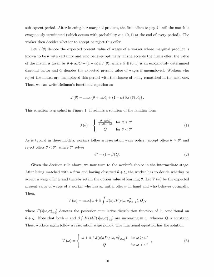
Thus, we can write Bellman’s functional equation as

() = max { + + (1− ) () } .

This equation is graphed in Figure 1. It admits a solution of the familiar form:

() =

⎧⎨⎩+1−(1−) for ≥ ∗

for ∗(1)

As is typical in these models, workers follow a reservation wage policy: accept offers ≥ ∗ and

reject offers ∗, where ∗ solves

∗ = (1− ). (2)

Given the decision rule above, we now turn to the worker’s choice in the intermediate stage.

After being matched with a firm and having observed + , the worker has to decide whether to

accept a wage offer and thereby retain the option value of learning . Let () be the expected

present value of wages of a worker who has an initial offer in hand and who behaves optimally.

Then,

() = max{ +

Z() (| 2|+) }

where (| 2+) denotes the posterior cumulative distribution function of , conditional on + . Note that both and

R() (| 2+) are increasing in , whereas is constant.

Thus, workers again follow a reservation wage policy. The functional equation has the solution

() =

⎧⎨⎩ + R() (| 2

|+) for ≥ ∗

for ∗, (3)

10

and the reservation wage, ∗, in the intermediate stage is implicitly defined by

∗ +

Z() (|∗ 2+) = . (4)

In equilibrium, the average accepted wage of workers in the intermediate stage is given by

[| ≥ ∗] =

R∞∗ (| 2)1−(∗| 2)

,

and that of tenured workers equals

[| ∗ ∗] =

R∞∗R∞∗ (| 2|+)(| 2)R∞

∗R∞∗ (| 2

|+) (| 2).

It is easy to verify that mean wages decrease when workers are willing to accept worse matches, i.e.

as reservation wages decline. In Appendix A, we show that ∗ ∗. Hence, on average wages rise

with tenure in the firm, whereas wages decrease as tenured workers lose their jobs and are being

rematched.

To close the model, the present discounted value of wages when unemployed is given by

=

Z () (| 2) + (1− ), (5)

where (| 2) denotes a normal cumulative distribution function with mean and variance

2 ≡ 4

2+2

.

Equations (1), (3), and (5) determine the worker’s optimal policy.

Introducing Racial Differences

The model above generalizes straightforwardly to incorporate a variety of differences in worker

characteristics. Indeed, each parameter in the set { 2 2} can vary by group identity.Because of this, there are many potential avenues to introduce racial disparities in wages. Note,

if groups differ on observable characteristics that are correlated with the parameters of the model,

then firms will treat each group of workers as if they belonged to a separate market of that type.

In particular, under the assumptions above it continues to be an equilibrium to pay each worker

her expected marginal product, given all available information (cf. Jovanovic 1979).11

11There exist many other equilibria. For instance, search frictions and the existence of market power may induce

firms to offer lower wages to groups of workers with lower reservation wages (Black 1995). Without free entry and

a perfectly elastic supply of entrepreneurs, biased employers may trade off profits for a desire to discriminate and

11

Disparities in the arrival rate of matches due, for example, to differences in search behavior or

discriminatory practices of firms can be captured by assuming that . This relationship is

reported in several audit studies in sociology and economics (e.g., Bendick et al. 1994, Pager 2003,

Bertrand and Mullainathan 2004). From equations (2) and (5) it is straightforward to show that

∗

0. That is, if blacks are less likely to receive job offers, then they also have lower reservation

wages and will accept worse matches. In equilibrium this results in racial wage gaps.

On the other hand, blacks and whites might be equally likely to obtain a match, but blacks

may be more likely to lose their job (see Fairlie and Kletzer 1998). Again, it is easy to show that

∗

0, which implies that increasing the chance of an exogenous separation lowers the reservation

wage. All else equal, this would result in lower wages for blacks. Moreover, disparities in arrival

and separation rates may lead to large racial differences in unemployment rates, as reported in

Stratton (1993).

Now, consider racial differences in the distribution of the match quality signal due to statistical

discrimination (Phelps 1972, Arrow 1973) or asymmetric screening technologies (Cornell and Welch,

1996, Lang 1986). In an Arrow (1973) model, the average of would differ between blacks and

whites, which results in racial differences in initial wage offers. Conversely, in a Phelps (1972) or

Aigner and Cain (1977) framework, the variance of is larger for blacks than for whites. In this

case, employers put more weight on average group ability when evaluating blacks’ signals than

when inferring the ability of a white candidate. While this will not lead to mean differences in if

both groups are equally skilled, if then black workers will, on average, receive lower wage

offers than whites with the same signal. In either case, our model predicts the black-white wage

gap to converge with tenure in the firm, since workers of equal ability earn the same wage after

their true ability has been revealed. As shown in subsequent sections, this prediction is, indeed,

born out in the data.

survive in equilibrium. One could also assume a Nash bargaining solution to set wages as in Eckstein and Wolpin

(1999). In order to fix ideas and keep focus on the core aspects of job search and learning, we choose to maintain the

simpler, more tractable–but admittedly less realistic–assumptions of Jovanovic (1979). The modelling exercise in

this paper is only designed to motivate the empirical work that follows.

12

4 Data and Econometric Approach

4.1 Data and Descriptive Statistics

The primary data set used in this paper was collected by the Princeton University Survey Research

Center (PSRC) during the fall of 2009 and early 2010.12 It is important to recognize that the

data were collected during a period of mass unemployment thereby lessening potiontial selection

problems into the pool of UI recipients (Gibbons and Katz 1991). Although we have do not have

compelling empirical evidence in favor of this assertion, it seems likely that layoffs during the 2009

recession were more random than during periods of a tight labor market.13

Starting from the universe of unemployment insurance (UI) recipients in the state of New Jersey

as of September 28, 2009, PSRC drew a stratified random sample of 63 813 currently unemployed

individuals. The sampled population was then contacted by the New Jersey Department of Labor

and Workforce Development (LWD) and invited to participate in a confidential web survey for a

period of 12 consecutive weeks.14

The survey consisted of an initial entry questionnaire and weekly follow-up interviews which

were remarkably rich. The former elicited information on demographics, previous employment, asset

holdings, and spouses’ employment status; whereas the latter inquired about job search activities,

time use, reservation wages, and job offers, among other topics. Participants were given the choice

of receiving an incentive payment of $20 within a few days of completing the entry questionnaire,

or $40 at the end of the 12 week survey period.

An important caveat to the data is that only 6 025 (roughly 10%) of the sampled individuals

participated in the entry wave, and those who responded to the initial survey completed only

about 40 percent of weekly follow-ups. The likelihood of responding varies by race. The sample of

respondents consisted of 153% blacks (compared to 186% in the sample frame) and 68% of whites

(relative to 617% in the sample frame).15 Participants were more educated, more likely to be

female, and had higher previous earnings than the baseline population. Using rich administrative

12 In what follows we draw heavily on Krueger and Mueller (2011). For a comprehensive description of the sampling

and interviewing procedures the interested reader should consult their appendix.13 In a seminal paper Gibbons and Katz (1991) argue that unemployed workers are negatively selected, and demon-

strate that wage losses following displacement are larger following layoffs than plant closings (which presumably pro-

vide little or no signal about worker ability). Recently, Hu and Taber (2011) have shown that this holds only among

white males, whereas blacks appear to suffer greater declines in wages following plant closings. Hu and Taber (2011)

rationalize this finding by appealing to heterogenous human capital.14 Individuals who were unemployed for 60 weeks or longer at the beginning of the survey were later asked to

participate in an additional 12 weeks of interviewing–for a maximum of 24 weeks. In this paper, however, we restrict

attention to the first 12 weeks for all respondents.15See Table 2.1 in Krueger and Mueller (2011).

13

data, Krueger and Mueller (2011) create sampling weights in order to adjust for the stratified

survey design as well as nonresponse. Comparing characteristics of respondents to the universe of

UI recipients along a number of dimensions — including those that were not used to construct the

weights (e.g. income, weekly exit rates from UI) — they conclude that the low response rate did

not significantly skew the sample on observables. After applying sample weights, blacks make up

20% of the sample (compared to 208% in the universe of UI recipients) and whites make up 598%

(compared to 589%).

Throughout our analysis we use the weights created by Krueger and Mueller (2011), and follow

their coding of wages by dropping wage offers below $5 an hour and offers above $100 per hour.

Moreover, we restrict attention to respondents with non-missing information on race who are not

listed as previously self-employed–for a final sample of 5 251 individuals. Appendix B provides

additional detail on the construction of our sample as well as precise definitions of all variables.

Summary statistics for the variables used in our main specifications are displayed, by race, in

Table 1, with ‘white’ referring solely to non-Hispanic whites. Our primary outcomes of interest are

offered wages and whether or not a job offer was received. Each of the follow-up surveys asked

whether respondents had received any job offer within the last 7 days, if so how many, and what

the wage associated with the best offer was.

In any given week about 65% of job seekers receive at least one job offer, and conditional upon

receiving any offer approximately 84% of individuals are offered exactly one job. Blacks write 13

more applications per week than whites, but are slightly less likely to apply for white collar jobs.16

Interestingly, and in contrast to results in the audit study literature, blacks have 22 percentage

points higher arrival rates than whites — at least in the raw data. However, the mean offered hourly

wage for whites equals $234, far in excess of the $123 offered to blacks. And differences in the

distribution of wage offers, as shown in Figure 2, are stark. The modal job offer is roughly the

same across racial groups, but the right tail of the white offer distribution is significantly larger. A

Kolmogrov-Smirnov test for equality in distributions is rejected at the 1%-level.

The remainder of Table 1 presents summary statistics for other variables used in our analysis.

About 45% of white, and 58% of black respondents are female. On average blacks are almost 7 years

younger than whites, and are much more likely to be single. Consistent with national patterns,

blacks in our sample are less educated than whites. For instance, about 32% of white respondents

16Pager and Pedulla (2011) report that blacks and whites apply to similar jobs, but blacks consider a greater range

of possibilities.

14

report to have at least a college education, compared to 17% for blacks.17 Blacks have longer

ongoing unemployment spells than whites, earned almost $400 less per week on their previous job,

and accumulated substantially less tenure than whites. We also have data on the industry in which

an individual previously worked. Blacks are less likely than whites to have worked in construction

and manufacturing. Instead, they are more concentrated in education and health care services.18

4.2 Identifying Discrimination

Four important features of the data described above enable us to conduct a novel test for racial

discrimination: information on wage offers (as opposed to just accepted wages), search strategies

and intensities, administrative data on previous earnings, as well as timing (the data were collected

during a period of mass unemployment). The key idea of our test is that, under the null hypothesis

of no discrimination, wages will closely proxy marginal productivity. Hence, conditional on wage

on the previous job, there should be no racial differences in wage offers, as controlling for previous

wage implicitly accounts for the market valuation of all factors such ability, non-cognitive skills, etc.

which previous research treated as unobservable. Therefore, observing racial differences in wage

offers after accounting for previous earnings would lead us to reject the null of no discrimination.

More formally, let denote the wage associated with the th job offer to individual and

consider the data generating process

ln () = 0 +0Γ0 + 00 + 0 + , (6)

where is an indicator variable for ’s race, are individual level covariates, denotes ’s

unobserved ability, and is white noise.19 Note that, although race and skill level will generally

be correlated, if employers do not discriminate it must be the case that Γ0 = 0.

Further assume that previous earnings, , are related to unobserved skill in the following sense:

= + ln () + 0 +

17Compared to unemployed New Jerseyites in the 2009 American Community Survey or the 2010 March CPS,

respondents in our data report broadly similar educational attainment; although self-reported dropouts are somewhat

under-represented and individuals with an incomplete college education are over-represented. It is important to note

that the numbers pertaining to educational achievement in Table 1 do not match those in Table 2.1 of Krueger and

Mueller (2011). In order to compare the sample of survey respondents to the universe of UI recipients they convert

adminstrative data on years of schooling (for both populations) into ‘degrees’, but rely on self-reported educational

attainment throughout the rest of their analysis.18Compared to the universe of UI recipients, construction workers are slightly under-represented in the weighted

data (Krueger and Mueller 2011).19We assume that skills command positive returns. That is, 0 ≥ 0

15

where 6= 0, [] = 0, Cov( ) = 0, and Cov (ln () ) = 0. This assumption is fairly

benign, as one can always write unobserved skill as a linear combination of previous earnings and

individual level covariates. In this case, corresponds to the least squares residual, which means

that [] = 0, and Cov (ln () ) = 0 are automatically satisfied. For 6= 0 to hold it needs tobe the case that even after controlling for previous wages predict ability, as seems likely.

20

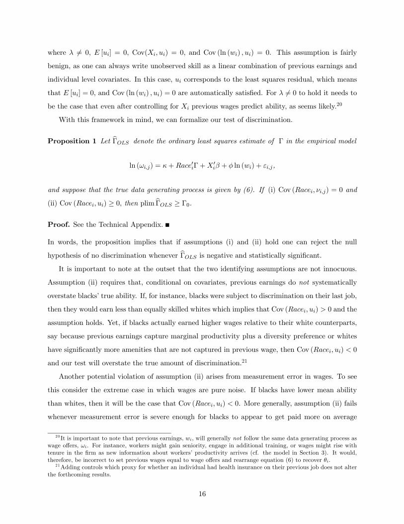
With this framework in mind, we can formalize our test of discrimination.

Proposition 1 Let bΓ denote the ordinary least squares estimate of Γ in the empirical model

ln () = +0Γ+ 0 + ln () + ,

and suppose that the true data generating process is given by (6). If (i) Cov ( ) = 0 and

(ii) Cov ( ) ≥ 0 then plim bΓ ≥ Γ0.Proof. See the Technical Appendix.

In words, the proposition implies that if assumptions (i) and (ii) hold one can reject the null

hypothesis of no discrimination whenever bΓ is negative and statistically significant.It is important to note at the outset that the two identifying assumptions are not innocuous.

Assumption (ii) requires that, conditional on covariates, previous earnings do not systematically

overstate blacks’ true ability. If, for instance, blacks were subject to discrimination on their last job,

then they would earn less than equally skilled whites which implies that Cov ( ) 0 and the

assumption holds. Yet, if blacks actually earned higher wages relative to their white counterparts,

say because previous earnings capture marginal productivity plus a diversity preference or whites

have significantly more amenities that are not captured in previous wage, then Cov ( ) 0

and our test will overstate the true amount of discrimination.21

Another potential violation of assumption (ii) arises from measurement error in wages. To see

this consider the extreme case in which wages are pure noise. If blacks have lower mean ability

than whites, then it will be the case that Cov ( ) 0. More generally, assumption (ii) fails

whenever measurement error is severe enough for blacks to appear to get paid more on average

20 It is important to note that previous earnings, , will generally not follow the same data generating process as

wage offers, . For instance, workers might gain seniority, engage in additional training, or wages might rise with

tenure in the firm as new information about workers’ productivity arrives (cf. the model in Section 3). It would,

therefore, be incorrect to set previous wages equal to wage offers and rearrange equation (6) to recover .21Adding controls which proxy for whether an individual had health insurance on their previous job does not alter

the forthcoming results.

16

than their equally skilled white counterparts. In an attempt to mitigate this concern, we use

administrative data on previous earnings, which is likely much more accurate than the usual self-

reported kind.22 In fact, administrative information usually serves as the benchmark in evaluation

studies of various surveys (see, for instance, Rodgers et al. 1993, Bound et al. 1994, as well as the

discussion in Bound et al. 2001).

The first assumption is that Cov ( ) = 0; which is automatically satisfied if is in

fact white noise. Intuitively, this assumption requires that, ceteris paribus, blacks and whites do not

systematically differ in their search behavior and draw wage offers from a comparable sets of firms.

If, for instance, blacks are more likely than whites to receive offers from firms particularly hard hit

by the 2009 recession–potentially because blacks are more concentrated in low level occupations–

then this assumption might be violated. Similarly, assumption (i) might fail if whites have lower

discount rates and firms’ adjust their offers accordingly, or if blacks do not bargain as aggressively

over offers as whites.

In contrast to the second assumption, however, assumption (i) is partially testable. Exploiting

the richness of our data we can account for racial differences in search strategies, search intensity,

geographic location, industry and occupation, bargaining behavior, as well as discounting. Although

there is little indication that differences along these lines explain our findings, we urge the reader

to keep these caveats in mind when interpreting the results presented below.

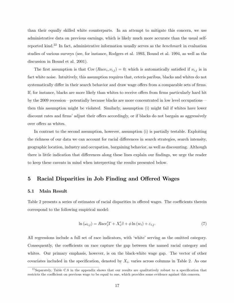
5 Racial Disparities in Job Finding and Offered Wages

5.1 Main Result

Table 2 presents a series of estimates of racial disparities in offered wages. The coefficients therein

correspond to the following empirical model:

ln () = 0Γ+ 0 + ln () + . (7)

All regressions include a full set of race indicators, with ‘white’ serving as the omitted category.

Consequently, the coefficients on race capture the gap between the named racial category and

whites. Our primary emphasis, however, is on the black-white wage gap. The vector of other

covariates included in the specification, denoted by , varies across columns in Table 2. As one

22Separately, Table C.8 in the appendix shows that our results are qualitatively robust to a specification that

restricts the coefficient on previous wage to be equal to one, which provides some evidence against this concern.

17

moves to the right, the set of covariates steadily grows. In all instances is the estimation carried

out using weighted least squares with weights corresponding to the sampling weights calculated by

Krueger and Mueller (2011). Standard errors are clustered by individual to account for the fact

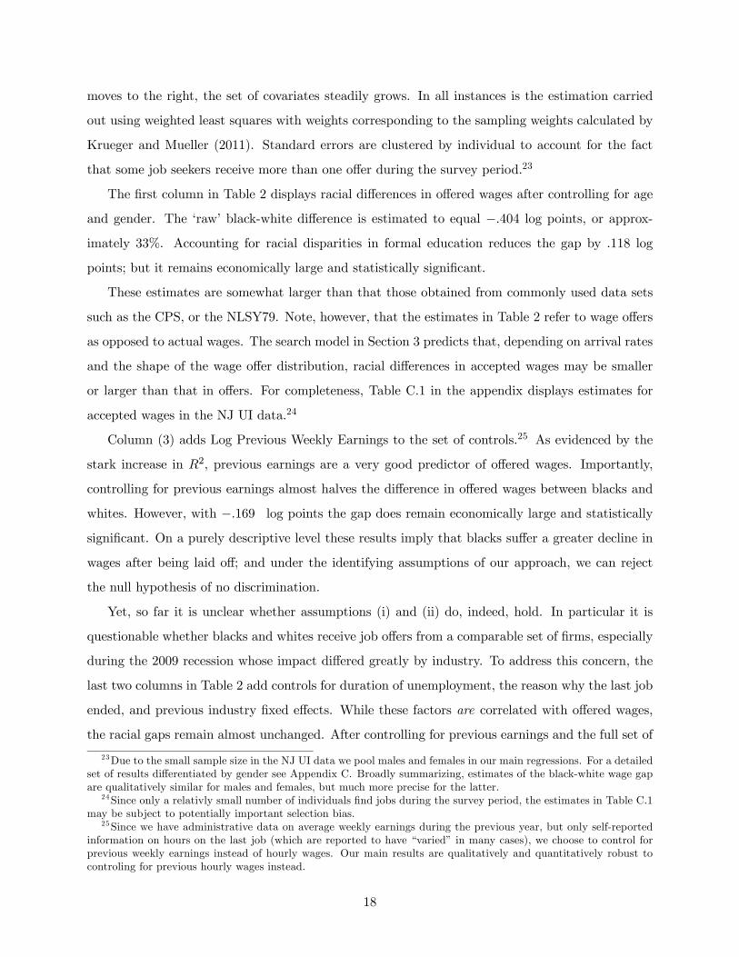
that some job seekers receive more than one offer during the survey period.23

The first column in Table 2 displays racial differences in offered wages after controlling for age

and gender. The ‘raw’ black-white difference is estimated to equal −404 log points, or approx-imately 33%. Accounting for racial disparities in formal education reduces the gap by 118 log

points; but it remains economically large and statistically significant.

These estimates are somewhat larger than that those obtained from commonly used data sets

such as the CPS, or the NLSY79. Note, however, that the estimates in Table 2 refer to wage offers

as opposed to actual wages. The search model in Section 3 predicts that, depending on arrival rates

and the shape of the wage offer distribution, racial differences in accepted wages may be smaller

or larger than that in offers. For completeness, Table C.1 in the appendix displays estimates for

accepted wages in the NJ UI data.24

Column (3) adds Log Previous Weekly Earnings to the set of controls.25 As evidenced by the

stark increase in 2, previous earnings are a very good predictor of offered wages. Importantly,

controlling for previous earnings almost halves the difference in offered wages between blacks and

whites. However, with −169 log points the gap does remain economically large and statistically

significant. On a purely descriptive level these results imply that blacks suffer a greater decline in

wages after being laid off; and under the identifying assumptions of our approach, we can reject

the null hypothesis of no discrimination.

Yet, so far it is unclear whether assumptions (i) and (ii) do, indeed, hold. In particular it is

questionable whether blacks and whites receive job offers from a comparable set of firms, especially

during the 2009 recession whose impact differed greatly by industry. To address this concern, the

last two columns in Table 2 add controls for duration of unemployment, the reason why the last job

ended, and previous industry fixed effects. While these factors are correlated with offered wages,

the racial gaps remain almost unchanged. After controlling for previous earnings and the full set of

23Due to the small sample size in the NJ UI data we pool males and females in our main regressions. For a detailed

set of results differentiated by gender see Appendix C. Broadly summarizing, estimates of the black-white wage gap

are qualitatively similar for males and females, but much more precise for the latter.24Since only a relativly small number of individuals find jobs during the survey period, the estimates in Table C.1

may be subject to potentially important selection bias.25Since we have administrative data on average weekly earnings during the previous year, but only self-reported

information on hours on the last job (which are reported to have “varied” in many cases), we choose to control for

previous weekly earnings instead of hourly wages. Our main results are qualitatively and quantitatively robust to

controling for previous hourly wages instead.

18

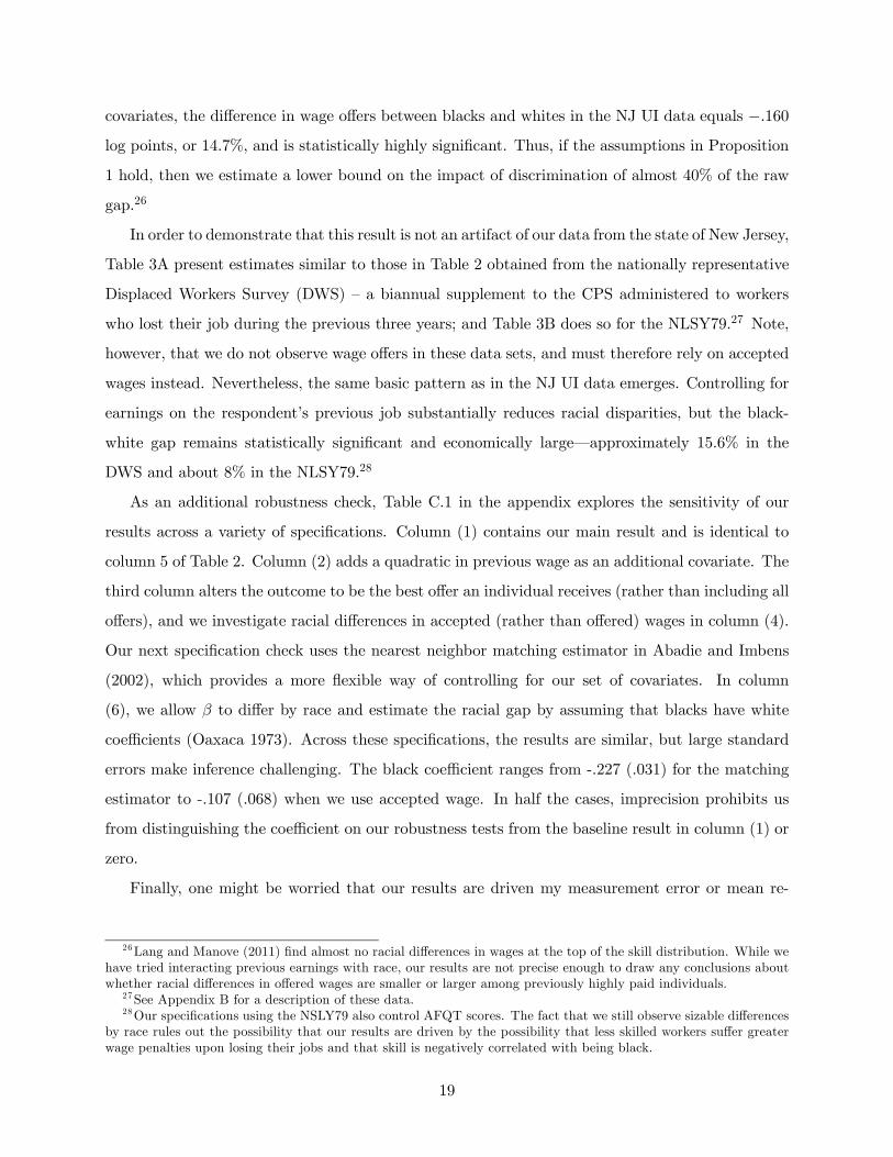
covariates, the difference in wage offers between blacks and whites in the NJ UI data equals −160log points, or 147%, and is statistically highly significant. Thus, if the assumptions in Proposition

1 hold, then we estimate a lower bound on the impact of discrimination of almost 40% of the raw

gap.26

In order to demonstrate that this result is not an artifact of our data from the state of New Jersey,

Table 3A present estimates similar to those in Table 2 obtained from the nationally representative

Displaced Workers Survey (DWS) — a biannual supplement to the CPS administered to workers

who lost their job during the previous three years; and Table 3B does so for the NLSY79.27 Note,

however, that we do not observe wage offers in these data sets, and must therefore rely on accepted

wages instead. Nevertheless, the same basic pattern as in the NJ UI data emerges. Controlling for

earnings on the respondent’s previous job substantially reduces racial disparities, but the black-

white gap remains statistically significant and economically large–approximately 156% in the

DWS and about 8% in the NLSY79.28

As an additional robustness check, Table C.1 in the appendix explores the sensitivity of our

results across a variety of specifications. Column (1) contains our main result and is identical to

column 5 of Table 2. Column (2) adds a quadratic in previous wage as an additional covariate. The

third column alters the outcome to be the best offer an individual receives (rather than including all

offers), and we investigate racial differences in accepted (rather than offered) wages in column (4).

Our next specification check uses the nearest neighbor matching estimator in Abadie and Imbens

(2002), which provides a more flexible way of controlling for our set of covariates. In column

(6), we allow to differ by race and estimate the racial gap by assuming that blacks have white

coefficients (Oaxaca 1973). Across these specifications, the results are similar, but large standard

errors make inference challenging. The black coefficient ranges from -.227 (.031) for the matching

estimator to -.107 (.068) when we use accepted wage. In half the cases, imprecision prohibits us

from distinguishing the coefficient on our robustness tests from the baseline result in column (1) or

zero.

Finally, one might be worried that our results are driven my measurement error or mean re-

26Lang and Manove (2011) find almost no racial differences in wages at the top of the skill distribution. While we

have tried interacting previous earnings with race, our results are not precise enough to draw any conclusions about

whether racial differences in offered wages are smaller or larger among previously highly paid individuals.27See Appendix B for a description of these data.28Our specifications using the NSLY79 also control AFQT scores. The fact that we still observe sizable differences

by race rules out the possibility that our results are driven by the possibility that less skilled workers suffer greater

wage penalties upon losing their jobs and that skill is negatively correlated with being black.

19

version in wages.29 A simple way to address this issue is to restrict the coefficient on previous

wage to equal one. If measurement error or mean reversion were, indeed, driving our results one

would expect the coefficient on race in the specification to equal zero. The result is presented in

column (7). The coefficient on black decreases 0049 log points (to −0111) and the standard errorincreases by more than 50% which leaves the black coefficient economically large but statistically

insignificant. It is unclear whether the differences between column (1) and column (7) of Table C.1

are due to true measurement error in the wages reported to the New Jersey Department of Labor

and Workforce Development or imposing restrictions on the data that are not warranted.30

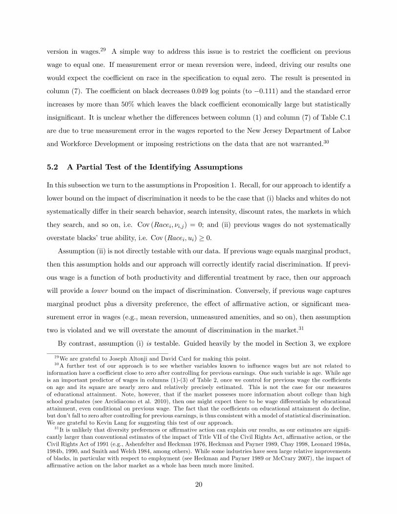
5.2 A Partial Test of the Identifying Assumptions

In this subsection we turn to the assumptions in Proposition 1. Recall, for our approach to identify a

lower bound on the impact of discrimination it needs to be the case that (i) blacks and whites do not

systematically differ in their search behavior, search intensity, discount rates, the markets in which

they search, and so on, i.e. Cov ( ) = 0; and (ii) previous wages do not systematically

overstate blacks’ true ability, i.e. Cov ( ) ≥ 0.Assumption (ii) is not directly testable with our data. If previous wage equals marginal product,

then this assumption holds and our approach will correctly identify racial discrimination. If previ-

ous wage is a function of both productivity and differential treatment by race, then our approach

will provide a lower bound on the impact of discrimination. Conversely, if previous wage captures

marginal product plus a diversity preference, the effect of affirmative action, or significant mea-

surement error in wages (e.g., mean reversion, unmeasured amenities, and so on), then assumption

two is violated and we will overstate the amount of discrimination in the market.31

By contrast, assumption (i) is testable. Guided heavily by the model in Section 3, we explore

29We are grateful to Joseph Altonji and David Card for making this point.30A further test of our approach is to see whether variables known to influence wages but are not related to

information have a coefficient close to zero after controlling for previous earnings. One such variable is age. While age

is an important predictor of wages in columns (1)-(3) of Table 2, once we control for previous wage the coefficients

on age and its square are nearly zero and relatively precisely estimated. This is not the case for our measures

of educational attainment. Note, however, that if the market posseses more information about college than high

school graduates (see Arcidiacono et al. 2010), then one might expect there to be wage differentials by educational

attainment, even conditional on previous wage. The fact that the coefficients on educational attainment do decline,

but don’t fall to zero after controlling for previous earnings, is thus consistent with a model of statistical discrimination.

We are grateful to Kevin Lang for suggesting this test of our approach.31 It is unlikely that diversity preferences or affirmative action can explain our results, as our estimates are signifi-

cantly larger than conventional estimates of the impact of Title VII of the Civil Rights Act, affirmative action, or the

Civil Rights Act of 1991 (e.g., Ashenfelter and Heckman 1976, Heckman and Payner 1989, Chay 1998, Leonard 1984a,

1984b, 1990, and Smith and Welch 1984, among others). While some industries have seen large relative improvements

of blacks, in particular with respect to employment (see Heckman and Payner 1989 or McCrary 2007), the impact of

affirmative action on the labor market as a whole has been much more limited.

20

five plausible violations of this assumption: spatial mismatch, racial differences in search behavior,

search strategies, bargaining, as well as discount rates. This constitutes only a partial test, given

there may be other factors leading to a positive correlation between and which we do

not observe in our data.

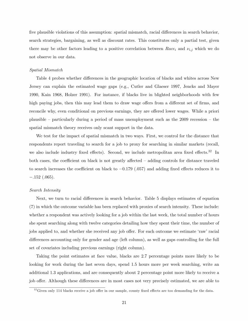
Spatial Mismatch

Table 4 probes whether differences in the geographic location of blacks and whites across New

Jersey can explain the estimated wage gaps (e.g., Cutler and Glaeser 1997, Jencks and Mayer

1990, Kain 1968, Holzer 1991). For instance, if blacks live in blighted neighborhoods with few

high paying jobs, then this may lead them to draw wage offers from a different set of firms, and

reconcile why, even conditional on previous earnings, they are offered lower wages. While a priori

plausible — particularly during a period of mass unemployment such as the 2009 recession — the

spatial mismatch theory receives only scant support in the data.

We test for the impact of spatial mismatch in two ways. First, we control for the distance that

respondents report traveling to search for a job to proxy for searching in similar markets (recall,

we also include industry fixed effects). Second, we include metropolitan area fixed effects.32 In

both cases, the coefficient on black is not greatly affected — adding controls for distance traveled

to search increases the coefficient on black to −0179 (057) and adding fixed effects reduces it to−152 (065).

Search Intensity

Next, we turn to racial differences in search behavior. Table 5 displays estimates of equation

(7) in which the outcome variable has been replaced with proxies of search intensity. These include:

whether a respondent was actively looking for a job within the last week, the total number of hours

she spent searching along with twelve categories detailing how they spent their time, the number of

jobs applied to, and whether she received any job offer. For each outcome we estimate ‘raw’ racial

differences accounting only for gender and age (left column), as well as gaps controlling for the full

set of covariates including previous earnings (right column).

Taking the point estimates at face value, blacks are 27 percentage points more likely to be

looking for work during the last seven days, spend 15 hours more per week searching, write an

additional 13 applications, and are consequently about 2 percentage point more likely to receive a

job offer. Although these differences are in most cases not very precisely estimated, we are able to

32Given only 114 blacks receive a job offer in our sample, county fixed effects are too demanding for the data.

21

rule out moderately sized gaps in favor of whites. Interestingly, blacks are significantly more likely

to report contacting employers directly, contacting public employment agencies, and using informal

networks. Thus, if anything, unemployed blacks appear to search more intensely for work across a

variety of channels and generate more offers than their white counterparts.

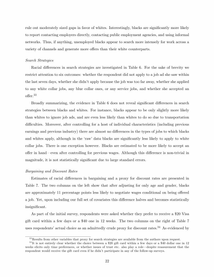
Search Strategies

Racial differences in search strategies are investigated in Table 6. For the sake of brevity we

restrict attention to six outcomes: whether the respondent did not apply to a job ad she saw within

the last seven days, whether she didn’t apply because the job was too far away, whether she applied

to any white collar jobs, any blue collar ones, or any service jobs, and whether she accepted an

offer.33

Broadly summarizing, the evidence in Table 6 does not reveal significant differences in search

strategies between blacks and whites. For instance, blacks appear to be only slightly more likely

than whites to ignore job ads, and are even less likely than whites to do so due to transportation

difficulties. Moreover, after controlling for a host of individual characteristics (including previous

earnings and previous industry) there are almost no differences in the types of jobs to which blacks

and whites apply, although in the ‘raw’ data blacks are significantly less likely to apply to white

collar jobs. There is one exception however. Blacks are estimated to be more likely to accept an

offer in hand–even after controlling for previous wages. Although this difference is non-trivial in

magnitude, it is not statistically significant due to large standard errors.

Bargaining and Discount Rates

Estimates of racial differences in bargaining and a proxy for discount rates are presented in

Table 7. The two columns on the left show that after adjusting for only age and gender, blacks

are approximately 11 percentage points less likely to negotiate wages conditional on being offered

a job. Yet, upon including our full set of covariates this difference halves and becomes statistically

insignificant.

As part of the initial survey, respondents were asked whether they prefer to receive a $20 Visa

gift card within a few days or a $40 one in 12 weeks. The two columns on the right of Table 7

uses respondents’ actual choice as an admittedly crude proxy for discount rates.34 As evidenced by

33Results from other variables that proxy for search strategies are available from the authors upon request.34 It is not entirely clear whether the choice between a $20 gift card within a few days or a $40 dollar one in 12

weeks elicits only time preferences, or whether issues of trust etc. also play a role–despite reassurement that the

respondent would receive the gift card even if he didn’t participate in any of the follow-up surveys.

22

point estimates of 22 and 156 percentage points, blacks are substantially more likely than whites

to opt for $20 now–suggesting that differences in time preferences may explain part of the gap, at

least if employers take these into account when making job offers.35

Understanding the Impact of Search Strategies, Search Intensity, Bargaining, and Discount Rates

Table 8 provides a concise summary of the effect of each of the five potential violations of

assumption (i). The estimates shown in the table correspond to the coefficient on , i.e. Γ in

specification (7), and denote racial differences in offered wages relative to whites. If assumption

(i) does indeed hold, then adding additional controls for each of the outcomes investigated above

should not decrease the gap in a statistically meaningful way.

The first column displays racial differences after accounting for the set of covariates used in

Table 2. Each subsequent column controls for one or more of the different dimensions of search

behavior explored in Tables 4—7. For instance, the second column also includes controls for whether

the respondent was looking for work during the last week, how many hours she spent searching,

and the number of applications she wrote. The third column adds indicator variables for whether

she didn’t apply to any job ad she saw within the last week, whether she did so because the job was

too far away, as well as whether she applied to a job opening in any of 22 Standard Occupational

Classification (SOC) Major Groups.

Despite the richness of the included covariates, the residual black-white difference in wage offers

remains almost unaffected. Separately accounting for the effect of search intensity, search strategies,

bargaining, time preferences, or geographic location reduces the gap by at most 033 log points–

compared to a standard error of 060. Even after jointly controlling for all of these factors, job offers

to blacks are still estimated to be 160 log points lower than those to observationally equivalent

whites.36

In sum, under the identifying assumptions of Proposition 1, we can conclude that discrimination

accounts for at least one third of the black-white wage gap.

6 Evidence Consistent with a Search-Matching Model

Recall, the search matching model in Section 3 has three stages. In the first stage unemployed

workers are stochastically matched with firms. After observing a productivity signal the firm offers

35Note, however, that such behavior might in itself be considered discriminatory.36This difference is strikingly similar in size to that reported in Lang and Manove (2011) for the NLSY79 after

controlling for education and AFQT.

23

a worker her expected marginal product, and the worker decides whether or not to accept the offer.

If she declines, she remains unemployed, but has a chance of being rematched in subsequent periods.

If the worker accepts, she works for one period, and in the following period both the worker and

the firm learn the true productivity of their match. Firms then offer a worker her match-specific

marginal product. The worker decides whether to continue the employment relationship (until an

exogenous separation occurs), or to enter unemployment and search for a better match.

As explained above, there are several ways to introduce racial differences into this framework.

If, for instance, blacks are on average less skilled than whites, i.e. (as documented by

Neal and Johnson 1996, among others), then group membership constitutes a valuable signal of

ability, and unemployed black workers will, on average, be offered lower initial wages than equally

qualified whites. In symbols, [ ] [].

There are three additional predictions of the model which are testable in our data. First, similar

to Black (1995), statistical discrimination in a search framework yields a lower reservation wage

for the disadvantaged group. Second, our model predicts the black-white wage gap to narrow

with tenure in the firm. Third, if blacks are significantly more likely than whites to experience

separations (as argued in Kletzer 1998), then aggregate wage gaps across firms will increase with

labor market experience. Below, we explore the extent to which these predictions are borne out in

the data.

Racial Differences in Reservation Wages

Table 9 presents evidence on racial differences in reservation wages (see Holzer 1986 for earlier

evidence). Reservation wages are gleaned from a question which asks, “Suppose someone offered

you a job today, what is the lowest wage or salary you would accept (before deductions) for the

type of work you are looking for.”37 It is important to note that differences in reservation wages

need not necessarily be due to discriminatory hiring practices. Instead, they might simply reflect

racial differences in discount rates or savings that could be used to smooth consumption while

unemployed (Chetty 2008).

The first column in Table 9 shows that, after accounting for age and gender, blacks are willing

to accept substantially lower offers than whites. The gap in reservation wages with these baseline

controls equals −232 log points. Accounting for educational achievement reduces the difference

37Krueger and Mueller (2011) report that whites are more likely than blacks to accept wage offers below their

stated reservation wage, which could be due to a variety of factors such as misinterpretation of the survey question

or individuals adjusting their reservation wage as they search.

24

to −160 log points, but it remains statistically significant. Similar to wage offers, earnings onthe previous job are a very good predictor of reservation wages. Moving from the second to the

third column 2 increases from 323 to 549, and reduces the black coefficient to −067 (.028).Put differently, on average, blacks are willing to accept almost 7% lower wages than whites who

previously earned just as much. Adding additional controls for the duration of unemployment, the

reason the last job ended, or previous industry fixed effects, does little to alter this result.

Returns to Tenure Within Firms

In our model, if blacks have lower mean pre-market skill this results in lower intermediate stage

wages for blacks. Over time, however, employers learn workers’ true marginal product which results

in no wage differences among equally productive tenured individuals. This provides a testable

prediction: within the firm, racial differences in wages should narrow with tenure.

Empirical evidence in support of this prediction is presented in Table 10. Using the NJ UI

data the table displays estimates of our empirical specification in which the outcome variable has

been replaced with the natural logarithm of previous earnings. Additionally, we control for tenure

on the previous job and interact it with race. As predicted, wages rise with tenure for all racial

groups. More importantly, however, blacks have a 11 percentage points higher return to tenure

than whites. Not only does the black-white difference in the return to tenure carry the expected

sign, it is also highly statistically significant.

A potential confounding factor of the above approach is that blacks are more likely than whites

to have short tenure and, as Topel (1991) shows, the returns to tenure are heavily weighted to

the first years on a job. Thus, the above analysis could be confusing non-linearities in the returns

to tenure as evidence in favor of the model. To test this possibility we divided tenure into four

categories: less than 2.5 years of experience, 2.5 to 5, 5 to 10, and more than 10 years. Interestingly,

the returns to tenure seem to be driven by black workers in the 10 or more years category.

Aggregate Racial Gaps Across Firms

In stark contrast to the previous discussion, when workers who have been with the same firm

for a sufficiently long time lose their job, the black-white wage gap re-emerges when these workers

are matched with a new firm. Thus, if blacks are sufficiently more likely than whites to incur a

separation, the black-white wage gap will increase with labor market experience. Altonji and Pierret

(2001) demonstrate that racial differences are small when workers just enter the labor market, but

widen with potential experience (see also Oettinger 1996).

25

Table 11 augments Altonji and Pierret’s (2001) original analysis of the NLSY79. The total

number of observations in Altonji and Pierret (2001) is 21,058 while that in our sample is 21,026.

This small difference is due to missing information on wages in the work history file of the NLSY79.

Nevertheless, our estimates are almost identical to theirs. For a detailed description of the sample

construction procedures see Appendix B, or the Data Appendix in Altonji and Pierret (2001).

Using data for the time period from 1979—92, columns (1)—(4) replicate the upper panel of their

Table 1. The negative coefficient on the interaction term between black and potential experience

indicates that the black-white wage widens by roughly 1% per year of experience.

In column (5) we extend Altonji and Pierret (2001) by adding tenure and its interaction with

race to the set of covariates. As predicted by our theory, blacks experience a 11 percentage points

higher return to tenure than whites. Not only is the difference statistically significant, it is also

surprisingly close to our estimate from the NJ UI data. The remainder of the table shows that this

result is robust to including additional years of data, and does not depend on Altonji and Pierret’s

(2001) choice to control for a cubic time trend interacted with black. Although the black-white

wage gap increases as individuals change employers and accumulate labor market experience, it is

estimated to be substantially smaller among those who have been with the same firm for a long

time.

7 Discussion

To conclude our analysis, we explore the extent to which discrimination based on animus or differ-

ences in pre-market skills can account for our set of facts: (1) blacks incur larger losses than whites

with job separations; (2) blacks have lower reservation wages; and (3) blacks garner higher returns

to tenure in a firm.

Taste-Based Discrimination

Discriminatory tastes of employers, co-workers, or customers can give rise to black-white wage

differences (Becker 1957). If, for instance, some fraction of employers incurs disutility from inter-

acting with black workers, then the wage offered to blacks must be lower than that of whites in

order for the employer to be indifferent. In equilibrium, the marginal discriminator determines the

black-white wage gap. Similar arguments apply when customers or co-workers discriminate based

on animus.38

38 In a rare empirical test of this theory Charles and Guryan (2008) argue that animus accounts for about one

26

The simplest models of taste-based discrimination can rationalize equilibrium wage gaps, but

have difficulty explaining why, after loosing their job, blacks are offered lower wages than previously

equally well paid whites. Unless the marginal discriminator changes during the year our data were

collected, controlling for previous earnings should eliminate the black-white wage gap — even in a

world where taste-based discrimination is present. This is inconsistent with what we find in the

data.

In contrast to neoclassical models of the labor market, models that include search frictions

such as Black (1995) predict that minorities will, on average, be paid lower wages as long as any

discriminatory employer is in the market. Expecting discrimination, blacks have lower reservation

wages than whites. Moreover, in a world with significant job specific human capital investment,

blacks may incur larger losses than white from job separations and have higher returns to tenure.

The key to this explanation is that blacks have more incentives to invest in firm specific human

capital because the market provides less insurance than it does for equally skilled whites.

Thus, our set of facts are consistent with a taste-based model of discrimination in which there

is substantial firm specific human capital investment. Lacking information on such investments, we

are unable to distinguish between taste-based and statistical flavors of discrimination.

Racial Differences in Pre-Market Factors

A separate strand of the literature relies on disparities in pre-market factors such as education

and skill to explain racial wage gaps.39 For instance, O’Neill (1990) as well as Neal and Johnson

(1996) show that after controlling for AFQT scores–which presumably measure skill prior to entry

into the labor market–the black-white wage difference in the NLSY79 narrows substantially or

even reverses. This theory finds mixed support in our data.

Racial differences in pre-market factors can explain racial differences in reservation wages. And,

to the extent that the price of skill increases with labor market experience or skill gaps widen with

labor market experience, then racial differences in pre-market factors can also explain why aggregate

wage gaps increase with age. Indeed, Altonji and Pierret (2001) demonstrate that the importance

of AFQT increases with labor market experience (see Table 11).

To explain why blacks incur a higher wage penalty from job separations than whites, one must

assume that there is a significant amount of firm specific investment among workers with low pre-

quarter of the observed black-white wage gap.39 It is theoretically unclear whether disparities in pre-market factors cause racial wage gaps, or whether the latter

lead minorities to invest less and thereby cause the former (see Lundberg and Startz 1983, or Coate and Loury 1993

for equilibrium analyses).

27

market skills. Moreover, a pre-market theory predicts that, conditional on AFQT, there are no

racial differences in the returns to tenure. This prediction is at odds with the data. Columns

(7) and (8) in Table 11 reveal that, conditional AFQT, blacks have significantly higher returns to

tenure than whites. Without controlling for AFQT, blacks have 11 percentage point higher returns

to tenure. Accounting for AFQT increases the coefficient to 12 percentage points.40 Given these

data, it is unlikely that pre-market factors alone explain the patterns in our data; although racial

differences in pre-market factors are likely important determinants of black-white inequality, and

may even give rise to statistical discrimination.

A Note on Statistical Discrimination and the Return to Education

Neal (2006) describes an important critique regarding the empirical content of models of statis-

tical discrimination, as developed by Arrow (1973) and Coate and Loury (1993). In these models,

blacks anticipate discrimination in the labor market and, expecting this, invest less in skills than

whites. Empirically, however, many have shown that the return to investment in skills is, if any-

thing, higher for blacks than whites which is inconsistent with simple versions the theory (e.g., see

Neal and Johnson 1996).

While we do not explicitly model investment in skills, there are several viable ways to incorporate

this critique into our theory. Generally, it is important to note that the return to education is

determined at the margin. That is, just because statistical discrimination causes blacks to earn on

average lower wages, does not necessarily mean that the function mapping educational investment

into earnings must be flatter. In equilibrium it will be the case that the gross return on investment

equals individuals’ opportunity cost (Becker 1962, 1993). Hence, if blacks are more likely to be cash

constrained or face higher cost of investing, then this alone may give rise to statistical discrimination

and explain higher estimated payoffs–assuming decreasing marginal returns.

More specifically, blacks may experience weakly higher returns on investment if education re-

duces the variance in the signal to employers (for empirical evidence see Arcidiacono et al. 2010);

which is, in fact, the assumption that drives the model in Lang and Manove (2011). In their analy-

sis blacks ‘overinvest’ in education to signal their (unobserved) ability. If depends not only on

group investments, but also on environmental factors such as school or neighborhood quality, then

in equilibrium it might well be the case that , despite higher returns for blacks.

An alternative way to rationalize higher returns for blacks is to assume that educational attain-

40Accounting for non-linearities in the returns to tenure by including years on the job in four categories, does not

alter this result.

28

ment decreases the probability of job loss (e.g., Kletzer 1998). In this case blacks would experience

a higher return to education than whites because it shields them from costly job losses.

***

The racial wage gap is a robust empirical regularity. Simple comparisons of mean wages typically

find black-white wage differences in excess of 30%. While there exists almost unanimous consensus

that differences in formal schooling and pre-market skill are important determinants of the observed

disparities, the extent to which discrimination contributes to the gap remains one of the most

debated issues in the social sciences.

In this paper we develop a novel test for the presence of discrimination using a newly available

dataset. Results from this test suggest that the impact of racial discrimination on offered wages

is at least one third of the raw black-white wage gap in our data — subject to our identifying

assumptions.

Taking our estimates at face value, labor market discrimination appears to be an impediment

to racial income equality. This suggests that alleviating racial inequality may take a combination

of policies to both eliminate barriers to investing in education and other premarket skills as well as

anti-discrimination enforcement so that minorities are rewared for those skills.

References

[1] Abadie, Alberto, and Guido W. Imbens (2002). “Simple and bias-corrected matching estima-

tors.” Unpublished Manuscript. University of California, Berkeley.

[2] Altonji, Joseph G., and Rebecca M. Blank (1999). “Race and Gender in the Labor Market,”

(pp. 3143—3259) in Orley C. Ashenfelter and David Card (eds.), Handbook of Labor Eco-

nomics, Vol. 3, Amsterdam: Elsevier

[3] Altonji, Jospeh G., and Charles R. Pierret (2001). “Employer Learning and Statistical Dis-

crimination,” Quarterly Journal of Economics, 116, 313—350.

[4] Aigner, Dennis J., Glen G. Cain (1977). “Statistical Theories of Discrimination in Labor

Markets,” Industrial and Labor Relations Review, 30, 175—187.

[5] Arcidiacono, Peter, Patrick Bayer, and Aurel Hizmo (2010). “Beyond Signaling and Human

Capital: Education and the Revelation of Ability,” American Economic Journal: Applied

Economics, 2, 76—104.

[6] Arrow, Kenneth J. (1973). “The Theory of Discrimination,” (pp. 3—33) in Orley C. Ashen-

felter and Albert Rees (eds.), Discrimination in Labor Markets, Princeton, NJ: Princeton

University Press.

29

[7] Ashenfelter, Orley C., and James J. Heckman (1976). “Measuring the Effect of an Antidiscrim-

ination Program,” in Orley C. Ashenfelter and James Blum (eds.), Evaluating the Labor

Market Effects of Social Programs, Princeton, NJ: Industrial Relations Section.

[8] Ayres, Ian, and Peter Siegelman (1995). “Gender and Race Discrimination in Bargaining for

a New Car,” American Economic Review, 85, 304—321.

[9] Becker, Gary S. (1957). The Economics of Discrimination. Chicago: University of Chicago

Press.

[10] Becker, Gary S. (1962). “Investment in Human Capital: A Theoretical Analysis,” Journal of

Political Economy, 70, 9—49.

[11] Becker, Gary S. (1993). Human Capital: A Theoretical and Empirical Analysis, with Special

Reference to Education. Chicago: University of Chicago Press.

[12] Bendick, Marc, Charles W. Jackson, and Victor A. Reinoso (1994). “Measuring Employment

Discrimination through Controlled Experiments,” Review of Black Political Economy, 23,

25—48.

[13] Bertrand, Marianne and Sendhil Mullainathan (2004) “Are Emily and Greg More Employable

than Lakisha and Jamal? A Field Experiment on Labor Market Discrimination,” American

Economic Review, 94, 991—1013.

[14] Black, Dan A. (1995). “Discrimination in an Equilibrium Search Model,” Journal of Labor

Economics, 13, 309—334.

[15] Black, Dan A., Natalia Kolesnikova, Seth G. Sanders, and Lowell J. Taylor (2010). “The Role

of Location in Evaluating Racial Wage Disparity,” Unpublished Manuscript, University of

Chicago.

[16] Blau, Francine D, and Andrea H. Beller (1992). “Black-White Earnings Over the 1970s and

1980s: Gender Differences in Trends,” Review of Economics and Statistics, 74, 276—286.

[17] Blendon, Robert J., Linda H. Aiken, Howard E. Freeman, and Christopher R. Corey (1989).

“Access to Medical Care for Black and White Americans,” Journal of the American Medical

Association, 261, 278—281.

[18] Blinder, Alan S. (1973) “Wage Discrimination: Reduced Form and Structural Estimates,”

Journal of Human Resources, 8, 435-455.

[19] Border, Kim (1996). “Partial Notes on a Simple Matching Model.” mimeo. California Institute

of Technology.

[20] Bound, John, Charles Brown, Greg J. Duncan, and Willard L. Rodgers (1994). “Evidence on

the Validity of Cross-Sectional and Longitudinal Labor Market Data,” Journal of Labor

Economics, 12, 345—368.

[21] Bound, John, Charles Brown, and Nancy Mathiowetz (2001). “Measurement error in survey

data,” (pp. 3705—3843) in James J. Heckman and Edward E. Leamer (eds.), Handbook of

Econometrics, Vol. 5, Amsterdam: Elsevier.

[22] Bowlus, Audra J. and Zvi Eckstein (2002). “Discrimination and Skill Differences in an Equi-

librium Search Model,” International Economic Review, 43, 1—38.

[23] Carneiro, Pedro, James J. Heckman, and Dimitriy V. Masterov (2005). “Labor Market Dis-

crimination and Racial Differences in Premarket Factors,” Journal of Law and Economics,

48, 1—39.

30

[24] Charles, Kerwin K., and Jonathan Guryan (2008). “Prejudice and Wages: An Empirical As-

sessment of Becker’s The Economics of Discrimination,” Journal of Political Economy, 116,

773—809.

[25] Charles, Kerwin K., and Jonathan Guryan (2011). “Studying Discrimination: Fundamental

Challenges and Recent Progress,” fortcoming in Annual Review of Economics.

[26] Chay, Kenneth Y. (1998). “The Impact of Federal Civil Rights Policy on Black Economic

Progress: Evidence from the Equal Employment Opportunity Act of 1972,” Industrial and

Labor Relations Review, 51, 608—632.

[27] Chetty, Raj (2008). “Moral Hazard vs. Liquidity and Optimal Unemployment Insurance,”

Journal of Political Economy, 116, 173—234.

[28] Coate, Stephen, and Glenn C. Loury (1993). “Will Affirmative-Action Policies Eliminate Neg-

ative Stereotypes?” American Economic Review, 83, 1220—1240.

[29] Coleman, James S. (1966). “Equality of Educational Opportunity.” US Department of Health,

Education, and Welfare, Office of Education.

[30] Cooper, Richard S., Joan F. Kennelly, Ramon Durazo-Arvizu, Hyun-Joo Oh, George Kaplan,

and John Lynch (2001). “Relationship between Premature Mortality and Socioeconomic

Factors in Black and White Populations of US Metropolitan Areas,” Public Health Reports,

116, 464—473.

[31] Corcoran, Mary and Greg J. Duncan (1979) “Work History, Labor Force Attachment, and

Earnings Differences between the Races and Sexes,” Journal of Human Resources, 14,

3—20.

[32] Cornell, Bradford, and Ivo Welch (1996). “Culture, Information, and Screening Discrimina-

tion,” Journal of Political Economy, 104, 542—571.

[33] Cutler, David M., and Edward L. Glaeser (1997). “Are Ghettos Good or Bad?” Quarterly

Journal of Economics, 112, 827-872.

[34] Darity, William A, and Patrick L. Mason (1998). “Evidence on Discrimination in Employment:

Codes of Color, Codes of Gender,” Journal of Economic Perspectives, 12, 63—90.

[35] Duncan, Greg J., Jeanna Brooks-Gunn, and Pamela K. Klebanov (1994). “Economic Depriva-

tion and Early Childhood Development,” Child Development, 65, 296—318.

[36] Greg J. Duncan (1999). Consequences of Growing Up Poor. New York: Russell Sage Founda-

tion.

[37] Eckstein, Zvi and Kenneth I. Wolpin (1999).“Estimating the Effect of Racial Discrimination

on First Wage Job Offers,” Review of Economics and Statistics, 81, 384—392.

[38] Esmail, Aneez, and Everington Sam (1993). “Racial Discrimination Against Doctors from

Ethnic Minorities,” British Medical Journal, 306, 691—692.

[39] Fairlie, Robert W., and Lori G. Kletzer (1998). “Jobs Lost, Jobs Regained: An Analysis

of Black/White Differences in Job Displacement in the 1980s,” Industrial Relations, 37,

460—477.

[40] Firth, Michael (1981). “Racial Discrimination in British Labour Market,” Industrial and Labor

Relations Review, 34, 265—272.

[41] Frisch, Ragnar, and Frederick V. Waugh (1933). “Partial Time Regressions as Compared with

Individual Trends,” Econometrica, 1, 387—401.

31

[42] Fryer, Roland G. (2011). “Racial Inequality in the 21st Century: The Declining Significance of

Discrimination,” (pp. 855—971) in Orley C. Ashenfelter and David Card (eds.), Handbook

of Labor Economics, Vol. 4, Amsterdam: Elsevier.

[43] Heckman, James J. (1998).“Detecting Discrimination.” Journal of Economic Perspectives 12,

101—116.

[44] Heckman, James J., and Brook S. Payner (1989). “Determining the Impact of Federal An-

tidiscrimination Policy on the Economic Status of Blacks: A Study of South Carolina,”

American Economic Review, 79, 138-177.

[45] Holzer, Harry (1986). “Reservation Wages and Their Labor Market Effects for Black and White

Male Youth,” Journal of Human Resources, 21, 157—177.

[46] Holzer, Harry (1991). “The Spatial Mismatch Hypothesis: What does the Evidence Show?”

Urban Studies, 28, 105—122.

[47] Hu, Luojia, and Christopher Taber (2011). “Displacement, Asymmetric Information, and Het-

erogeneous Human Capital,” Journal of Labor Economics, 29, 113—152.

[48] Jencks, Christopher, and Susan Mayer (1990.) “Residential Segregation, Job Proximity, and

Black Opportunities,” (pp. 187—222) in Laurence E. Lynn and Michael G.H. McGeary

(eds), Inner City Poverty in the United States, Washington, DC: National Academy Press.

[49] Jovanovic, Boyan (1979). “Job Matching and the Theory of Turnover,” Journal of Political

Economy, 87, 972—990.

[50] Kain, John D. (1968). “Housing Segregation, Negro Employment, and Metropolitan Decen-

tralization,” Quarterly Journal of Economics 82, 175—19.

[51] Kletzer, Lori G. (1998). “Job Displacement,” Journal of Economic Perspectives, 12, 115—136.

[52] Krueger, Alan B., and Andreas Mueller (2011). “Job Search and Job Finding in a Period of

Mass Unemployment: Evidence from High-Frequency Longitudinal Data,” Working Paper

#562, Industrial Relations Section, Princeton University.

[53] Lang, Kevin (1986). “A Language Theory of Discrimination,” Quarterly Journal of Economics,

101, 363—382.

[54] Lang, Kevin, and Jee-Yeon K. Lehmann (2010). “Racial Discrimination in the Labor Market:

Theory and Empirics,” Unpublished Manuscript, Boston University.

[55] Lang, Kevin, and Michael Manove (2011). “Education and Labor Market Discrimination,”

American Economic Review, 101, 1467—1496.

[56] Leonard, Jonathan S. (1984a). “The Impact of Affirmative Action on Employment,” Journal

of Labor Economics, 2, 439—463.

[57] Leonard, Jonathan S. (1984b). “Employment and Occupational Advance Under Affirmative

Action,” Review of Economics and Statistics, 66, 377—385.

[58] Leonard, Jonathan S. (1990). “The Impact of Affirmative Action Regulation and Equal Em-

ployment Law on Black Employment,” Journal of Economic Perspectives, 4, 47-63

[59] List, John A. (2004). “The Nature and Extent of Discrimination in the Marketplace: Evidence

from the Field,” Quarterly Journal of Economics 119, 49—89.

[60] Lundberg, Shelly J., and Richard Startz (1983). “Private Discrimination and Social Interven-

tion in Competitive Labor Market,” American Economic Review, 73, 340—347.

32

[61] McCrary, Justin (2007). “The Effect of Court-Ordered Hiring Quotas on the Composition and

Quality of Police,” American Economic Review, 97, 318—353.

[62] Neal, Derek A. (2006). “Why Has Black-White Skill Convergence Stopped?,” (pp. 511—576) in

Eric A. Hanushek and Finis Welch (eds.), Handbook of the Economics of Education, Vol.

1, Amsterdam: Elsevier.

[63] Neal, Derek A. (2004). “The Measured Black-White Wage Gap Among Women Is Too Small,”

Journal of Political Economy, 112, S1-S28.

[64] Neal, Derek A., and William R. Johnson (1996). “The Role of Premarket Factors in Black-

White Wage Differences,” Journal of Political Economy, 104, 869—895.

[65] Neumark, David, Roy J. Bank, and Kyle D. Van Nort (1996). “Sex Discrimination in Restau-

rant Hiring: An Audit Study,” Quarterly Journal of Economics, 111, 915—941.

[66] Oaxaca, Ronald L. (1973). “Male-Female Wage Differentials in Urban Labor Markets,” Inter-

national Economic Review, 14, 693-709.

[67] Oaxaca, Ronald L., and Michael R. Ransom (1994). “On Discrimination and the Decomposi-

tion of Wages,” Journal of Econometrics, 61, 5—21.

[68] Oettinger, Gerald S. (1996). “Statistical Discrimination and the Early Career Evolution of the

Black-White Wage Gap,” Journal of Labor Economics, 14, 52—78.

[69] O’Neill, June (1990). “The Role of Human Capital in Earnings Differences Between Black and

White Men,” Journal of Economic Perspectives, 4, 25—45.

[70] Pager, Devah (2003). “The Mark of a Criminal Record,” American Journal of Sociology, 108,

937—975.

[71] Pager, Devah (2007). “The Use of Field Experiments for Studies of Employment Discrimina-

tion: Contributions, Critiques, and Directions for the Future.” Annals of the American

Academy of Political and Social Science, 609, 104-133.

[72] Pager, Devah, Bruce Western, and Bart Bonikowski (2009). “Discrimination in a Low-Wage

Labor Market: A Field Experiment,” American Sociological Review, 74, 777—799.

[73] Phelps, Edmund S. (1972). “The Statistical Theory of Racism and Sexism,” American Eco-

nomic Review, 62, 659—661.

[74] Prescott, Edward C., and Robert M. Townsend (1980). “Equilibrium under Uncertainty: Mul-

tiagent Statistical Decision Theory,” (pp. 169—194) in Arnold Zellner (ed.), Bayesian Analy-

sis in Econometrics and Statistics, Amsterdam: North-Holland.

[75] Reimers, Cordelia (1983) “Labor Market Discrimination Against Hispanic and Black Men,”

Review of Economics and Statistics, 65, 570—579.

[76] Riach, Peter A., and Judith Rich (2002). “Field Experiments of Discrimination in the Market

Place,” Economic Journal, 112, F480—F518.

[77] Rodger, Willard L., Charles Brown, and Greg J. Duncan (1993). “Errors in Survey Reports of

Earnings, Hours Worked, and Hourly Wages,” Journal of the American Statistical Associ-

ation, 88, 1208—1218.

[78] Sargent, Thomas J. (1987). Dynamic Macroeconomic Theory. Cambridge, MA: Harvard Uni-

versity Press.

[79] Smith, James P., and Finis R. Welch (1984). “Affirmative Action and Labor Markets,” Journal

of Labor Economics, 2, 269—301

33

[80] Smith, James P., and Finis R. Welch (1986). Closing the Gap: Forty Years of Economic

Progress for Blacks. Santa Monica: RAND.

[81] Stratton, Leslie S. (1993). “Racial Differences in Men’s Unemployment,” Industrial and Labor

Relations Review, 46, 451—63.

[82] Turner, Margery A., Michael Fix, and Raymond J. Struyk (1991). Opportunities Denied, Op-

portunities Diminished: Racial Discrimination in Hiring. Washington, DC: Urban Institute

Press.

[83] Western, Bruce, Meredith Kleykamp, and Jake Rosenfeld (2006). “Did Falling Wages and

Employment Increase U.S. Imprisonment,” Social Forces, 84, 2291—2311.

[84] Williams, David R. and Pamela B. Jackson (2005). “Social Sources of Racial Disparities in

Health.” Health Affairs, 24, 325—334.

[85] Wolpin, Kenneth I. (1992). “The Determinants of Black-White Differences in Early Employ-

ment Careers: Search, Layoffs, Quits, and Endogenous Wage Growth,” Journal of Political

Economy, 100, 535—560.

34

A Technical Appendix

In this appendix, we provide formal proofs for the results stated in the main text.

Proof of Proposition 1. Replacing in (6) with = + ln ()+ 0+ yields the estimable

specification

ln () = (0 + 0) +0Γ0 + 0 (0 + 0) + 0 ln () + (0 + ) ,

in which only (0 + ) is not observed by the econometrician.

The Frisch-Waugh Theorem (Frisch and Waugh 1933) implies that

plim bΓ = Γ0 + Cov³̂ 0 +

´Var

³̂

´ ,

where ̂ denotes the residual from projecting onto , ln (), and a constant. Since

Var³̂

´ 0, it suffices to show that Cov

³̂ 0 +

´≥ 0.

From the definition of ̂ and using the Frisch-Waugh Theorem again one obtains:

Cov³̂ 0 +

´= Cov

à − − 0

Cov(f)

Var(f)− Cov( l̂n ())

Var(l̂n ())ln () 0 +

!

where ≡ []−[ 0]Cov()

Var()− Cov(l̂n())

Var(l̂n())[ln ()], and f (l̂n ()) corresponds

to the residual from projecting (ln ()) onto ln () () and a constant. Since ⊥( )as well as ln ()⊥( ), we have that Cov

³̂ 0 +

´= Cov ( 0 + ). As-

sumptions (i) and (ii) in Proposition 1 ensure that Cov ( 0 + ) ≥ 0. Hence, plim bΓ ≥Γ0, as desired.

Proposition 2 The sequence of reservation wages is increasing, i.e. ∗ ∗.

Proof. Note that Pr [ ∗| + ] 0 and () ≥ with the inequality being strict for ∗.

It then follows that

∗ +

Z() (|∗ 2|+) ∗ + .

Hence, equation (4) implies ∗ (1− ) . Recognizing that ∗ = (1− ) by (2) completes the

proof.

35

Proposition 3 On average wages increase with tenure in the firm. That is, [| ∗]

[| ∗ ∗].

Proof. For completeness we reproduce the proof contained in Sargent (1987, pp. 79).

First, note that the mean wage of previously unemployed workers is given by

[| ∗] ≡ =

R∞∗ (| 2)R∞∗ (| 2)

,

and that of tenured workers equals

[| ∗ ∗] ≡ =

R∞∗R∞∗ (| 2

|+) (| 2)R∞∗

R∞∗ (| 2

|+) (| 2).

From the standard properties of normally distributed random variables it follows that

= +

³−∗

´Φ³−∗

´ .Moreover, since

R∞∗ (| 2

|+) = Φ³

−∗|+

´, we also have that

Z ∞

∗ (| 2|+) = Φ

µ − ∗

|+

¶+

µ − ∗

|+

¶ Φ

µ − ∗

|+

¶.

This implies

R∞∗ Φ

³−∗|+

´(| 2)R∞

∗ Φ³

−∗|+

´(| 2)

≡ e.Hence, it suffices to show that e ≥ .

Next, let (| 2) denote the probability density function associated with (| 2), andnote that the density of observed wages in the second stage is given by:

e(| 2) =⎧⎨⎩

(|2)∞∗ (|2) if ≥ ∗

0 if ∗.

36

Similarly, define

ee(| 2) =⎧⎪⎪⎪⎨⎪⎪⎪⎩

Φ

−∗|+

(|2)∞

∗ Φ

−∗|+

(|2)

if ≥ ∗

0 if ∗

,

and let e(| 2) and ee(| 2) denote the cumulative distribution functions associated withe(| 2) and e(| 2), respectively.By construction,

=

Z ∞

∗ e(| 2) = ∗ +

Z ∞

∗1− e(| 2) (8)

e = Z ∞

∗

ee(| 2) = ∗ +Z ∞

∗1− ee(| 2) (9)

as well as

ee(| 2) = Φ³

−∗|+

´ R∞∗ (| 2)R∞

∗ Φ³

−∗|+

´(| 2)

e(| 2).As, for ∗ −∞, Φ

³−∗|+

´is strictly increasing in and both ee(| 2) and e(| 2) are

probability densities, it must be the case that there exists exactly one 0 ∗ such that ee(| 2) ≷e(| 2) whenever ≷ 0. To see this note thatR∞∗ (| 2)

R∞∗ Φ

³−∗|+

´(| 2)

and that 0 ≤ Φ³

−∗|+

´≤ 1. Thus, e(| 2) ee(| 2) for sufficiently large . Also, recall

that e(00| 2) = ee(| 2) = 0 for ∗. The fact that Φ³

−∗|+

´is strictly increasing implies

that(|2)(|2) is strictly increasing as well (for ≥ ∗). Since both densities have to integrate up

to one, we have that e(∗| 2) ee(∗| 2) and that the density functions cross only once.Therefore,

ee(| 2) e(| 2) for 0. From (8) and (9) it then follows that e ,

which completes the proof.

Proposition 4 Lower arrival rates result in lower reservation wages, i.e. ∗

0.

Proof. By (2) it suffices to show that

0. Rearranging (5) and taking the derivative with

respect to gives

=

(1− )

(1− (1− ))2

Z ()

¡| 2

¢+

1− (1− )

Z ()

¡| 2

¢. (10)

37

From the definition of () it follows that, for all ,

()

≥ min{

Z ()

³| 2|+

´

}; (11)

and from equation (1) we have that

()

≥ min{

1− (1− )

}

for all .

Case 1: Suppose

0. Then, as 0 1−(1−) 1,

()≥

. Thus, by (11) we have that

()≥

.

Since the distribution of is nondegenerate normal and agents can always refuse negative offers,

() 0 for all . Therefore,

1− (1− )

Z ()

¡| 2

¢ ≥

1− (1− )

. (12)

Letting ≡ 1−(1−) and rearranging (12) gives

(1− )

0,

which produces a contradiction, as 0 1.

Case 2: Suppose ≥ 0. Then,

()≥

1−(1−)and

()

≥ 2

1−(1−). In this case,

equation (12) becomes

1− (1− )

2

1− (1− )

.

Again, letting ≡ 1−(1−)

2

1−(1−) and rearranging gives

(1− )

0. (13)

Note that 0 1. Hence, (13) demonstrates that

0, as desired.

Proposition 5 A higher probability of job loss results in lower reservation wages, i.e. ∗

0.

38

Proof. By (2) it suffices to show that

0. Rearranging (5) and taking the derivative with

respect to gives

=

1− (1− )

Z ()

¡| 2

¢. (14)

From the (3) we have that, for all ,

()

≤ max{

Z ()

³| 2|+

´

}; (15)

and from the definition of , i.e. () = max { + + (1− ) () }, it follows that either

()

=

1− (1− )(− ()) +

1− (1− )

(16)

or

()

=

.

Since () ≥ for all , it must be the case that()≤ max{

1−(1−) }.

Case 1: Suppose

0. Then, as 0 1−(1−) 1,

()≤

. Thus, by (15) we have that

()≤

.

This and (14) imply

≤

1− (1− )

. (17)

Letting ≡ 1−(1−) and rearranging (17) gives

(1− )

≤ 0,

which produces a contradiction, since 0 1.

Case 2: Suppose ≤ 0. Then, as 0

1−(1−) 1,()≤

1−(1−). Thus, by (15) we have

that ()≤ 2

1−(1−).

In this case equation (17) becomes

≤

1− (1− )

2

1− (1− )

.

Letting ≡ 1−(1−)

2

1−(1−) and rearranging gives

(1− )

≤ 0. (18)

39

Note that 0 1. Hence, (18) demonstrates that ≤ 0.

It remains to be shown that 6= 0. By way of contradiction, suppose

= 0. Then,

()≤ 0

with the inequality being strict for large enough (due to (16) and the fact that () for large

). From (3) we have that ()≤ 0, again with the inequality being strict for large enough.

This in connection with (14) implies that

0, which produces the desired contradiction.

B Data Appendix

B.1 NJ UI Data

The following description of the NJ UI data borrows heavily from Krueger and Mueller (2011).

For a more detailed description of the data (in particular of the sampling procedures, the survey

instrument, or details of the implementation) the interested reader should consult their appendix.

During the fall of 2009 and early 2010 the Princeton University Survey Research Center (PSRC)

collected high-frequency longitudinal information on the unemployed in the state of New Jer-

sey. Starting from a complete list of the approximately 360,000 individuals receiving unemploy-

ment insurance (UI) as of September 28, 2009, PSRC drew a stratified random sample of 63,813

individuals–oversampling the long-term unemployed. The sampled population was then contacted

by the New Jersey Department of Labor and Workforce Development (LWD) and invited (by email

or letter) to participate in a confidential web survey for a period of 12 consecutive weeks. Individu-

als who were unemployed for 60 weeks or longer at the beginning of the survey were later asked to

participate in an additional 12 weeks of interviewing–for a maximum of 24 weeks. In this paper,

however, we restrict attention to the first 12 weeks for all respondents.

Six to ten days after the initial invitation, PSCR made almost 10,000 phone calls encouraging

non-responders to participate in the survey. Two weeks thereafter the survey was closed for new

participants. In order to remind respondents to participate in the weekly follow-up surveys e-mail

invitations were sent out seven days after completion of the most recent online interview, but not

on Sundays or Mondays.41

As incentive to participate respondents could choose between a $20 Visa gift card mailed to

them within a few days, or a $40 one sent out after the 12 week survey period–regardless of

whether the respondent would complete any follow-up interviews.

41This restriction was imposed so the time diary would pertain to a weekday. Respondents who completed their

most recent survey on a Sunday would receive their invitation on Tuesday of the following week.

40

The actual survey consisted of an initial entry questionnaire and weekly follow-up interviews.

The former elicited information on demographics, previous employment, asset holdings, and spouses’

employment status; whereas the latter inquired about job search activities, time use, reservation

wages, and job offers, among other topics. Participants were given the choice of receiving an incen-

tive payment of $20 within a few days of completing the entry questionnaire, or $40 at the end of

the 12 week survey period.

Unfortunately, only 6,025 of the sampled individuals participated in the entry wave of the survey,

and those who responded to the initial interview completed only about 40 percent of weekly follow-

ups. Moreover, participants were more educated, more likely to be female, and had higher previ-

ous earnings than the baseline population. Using rich administrative data, Krueger and Mueller

(2011) create sampling weights in order to adjust for the stratified survey design as well as nonre-

sponse. Comparing characteristics of respondents to the universe of UI recipients along a number

of dimensions, they conclude that the low response rate did not significantly skew the sample on

observables–even on those that were not used in calculating the weights. Throughout our analysis

we use the weights created by Krueger and Mueller (2011). Moreover, we restrict attention to

respondents with non-missing information on race who are not listed as previously self-employed.

Our final sample consists of 5,251 individuals and 26,901 person-week observations.

The following variables are used throughout our analysis:

Race is a set of mutually exclusive indicator variables, i.e. White, Black, Hispanic, Asian, and

Other Race, that denote a respondent’s racial identification. In our regressions White serves as the

omitted category.

Female is an indicator variable that equals one if the respondent is female and zero otherwise.

Age denotes the respondent’s age in years.

Number of Children denotes the respondent’s number of children. The variable is taken from

the entry questionnaire which asked “How many children do you have?”

Marital Status is a set of mutually exclusive indicator variables, i.e. Single, Married, Divorced,

Widowed, and Cohabitating But Not Married, that denote a respondent’s marital status. The

information is taken from the entry questionnaire which asked “What is your marital status?” The

41

set of possible answers was: “Single (Never Married)”, “Married”, “Divorced”, “Widowed”, and

“Domestic partnership (living together but not married)”.

Educational Attainment is a set of mutually exclusive indicator variables, i.e. High School

Dropout, High School Graduate, Some College, and College Graduate, that denote a respondent’s

highest level of completed education. The information is taken from the entry questionnaire which

asked “What is the highest level of education you have completed?” The set of possible answers

was: “Some high school or less”, “High school diploma or equivalent”, “Some college”, “College

diploma”, “Some graduate school”, “Graduate degree”. For the purposes of this paper we combine

the last three answer choices into one category.

Weeks Unemployed denotes the duration of a respondent’s unemployment spell as of the time

she filled out a weekly follow-up survey. The variable has been constructed using information on

the time she lost her main job, i.e. the one at which she worked the most hours, from the entry

questionnaire as well as on the time she filled out the weekly survey.

Previous Weekly Earnings denotes the respondent’s average weekly earnings during the past

year. This variable has been constructed using administrative information form the New Jersey

Department of Labor and Workforce Development on earnings and weeks worked in the base year.

Following Krueger and Mueller (2011) we discard observation with weekly earnings of less than

$100 or more than $8,000, and impute base year earnings of $152,191 for those individuals subject

to top-coding.

Tenure on Previous Job denotes the time (in years) that the respondent worked for her previous

employer. The variable is taken from the entry questionnaire which asked “How many years had

you worked for that employer when that job ended?”

Reason Last Job Ended is a set of mutually exclusive indicator variables, i.e. Quit Last Job,

Laid Off from Last Job, and Last Job was Temporary, which denote why the respondent’s last job

ended. The information is taken from the entry questionnaire which asked “Did you lose or quit

that job, or was it a temporary job that ended?” The set of possible answers was: “Lost job”,

“Quit Job”, and “Temporary Job ended”. In our regressions Laid Off from Last Job serves as the

omitted category.

42

Previous Industry refers to a set of nine indicator variables categorizing the industry in which

participants previously worked according to the North American Industry Classification System

(NAICS).

Received Offer Last Week is an indicator variable for whether the respondent reports having

received at least one job offer during the previous seven days. The variable is taken from the

weekly follow-up surveys which asked “In the last 7 days, did you receive any job offers? If yes,

how many?”

Offered Hourly Wage denotes the pay associated with the best job offer the respondent re-

ceived within the last seven days, converted into an hourly rate. To construct this variable we use

information from the weekly follow-up surveys which asked “What was the wage or salary offered

(before deductions)? Is that per year, per month, bi-weekly, weekly or per hour?” and “How many

hours a week would you have to work on that job?”. We discard observations with missing informa-

tion on hours, and, following Krueger and Mueller (2011), observations with hourly offered wages

of less than $5 or more than $100.

Accepted Job Offer in Hand is an indicator variable equal to one if the respondent accepted

or thinks she will accept the best offer received within the last seven days. The variable is taken

from the weekly follow-up surveys which asked “Have you accepted or do you think you will accept

this job offer?” The set of possible answers was: “Yes”, “No”, “Don’t know yet”. Only respondents

answering “Yes” are coded as one; those who say “Don’t know yet” are set to missing.

Accepted Hourly Wage denotes the hourly wage associated with job offered that the respon-

dent accepted, if she in fact did accept one. The variable is coded in the same way as the two

previous ones.

Looking for Job Last Week is an indicator variable equal to one if the respondent was actively

looking for work during the previous seven days. The variable is taken from the weekly follow-up

surveys which asked “Have you done anything to find work during the last 7 days?”.

Hours Spent Searching denotes the total number of hours the respondent claims to have spent

trying to find a job. The variable is constructed using information from the weekly follow-up sur-

veys which asked “On the previous page you indicated what kind of methods you used to find work.

43

In the last 7 days, about how many hours and minutes did you spend on each of those methods?

Your best guess is okay.” The set of methods included: “Contacted employer directly”, “Contacted

public employment agency”, “Contacted private employment agency”, “Contacted friends or rela-

tives”, “Contacted school/university employment center”, “Checked union/professional registers”,

“Attended job training programs/courses”, “Placed or answered ads”, “Went to interview”, “Sent

out resumes/filled out applications,” “Looked at ads,” “Other”.

Number of Applications denotes the number of jobs to which the respondent applied within

the last seven days. The variable is taken from the weekly follow-up surveys which asked “How

many jobs did you apply to in the last 7 days?”

Didn’t Apply to Some Job Ad Last Week is an indicator variable equal to one if the

respondent did not apply to any job for which she was qualified–for any reason. The variable is

constructed using information from the weekly follow-up surveys which asked “What about jobs

you did not apply for? Did you find or hear about any jobs in the last 7 days for which you are

qualified but did not apply for?”

Didn’t Apply Since Too Far Away is an indicator variable equal to one if the respondent did

not apply to any job for which she was qualified because it was too far away, and equal to zero

if she did not apply for any other reason. The variable is constructed using information from the

weekly follow-up surveys which asked “What about jobs you did not apply for? Did you find or

hear about any jobs in the last 7 days for which you are qualified but did not apply for?” and “Why

not? Please check all that apply.”

Applied to Any White Collar Job Last Week is an indicator variable equal to one if the

respondent applied to a white collar job within the last seven days and zero otherwise. The variable

has been constructed using information from the weekly follow-up surveys which asked “Please list

the three most recent jobs you applied to in the last 7 days. If you applied to more than one of the

same kind of job, list each job separately. (examples of job titles include: waiter, computer techni-

cian, warehouse worker, administrative assistant, etc.)” The answers in the text entry fields were

then categorized into Standard Occupational Categories (SOC) by trained staff at the University of

Wisconsin Survey Center. 97% of job titles could be successfully matched to 3-digit SOC codes. We

code the following 2000 Major Groups as ‘white collar’: “Management”, “Business and Financial

44

Operations”, “Computer and Mathematical Occupations”, “Office and Administrative Support”,

“Architecture and Engineering”, “Life, Physical, and Social Science”, “Community and Social

Services”, “Legal Occupations”, “Education, Training, and Library Occupations”, “Arts, Design,

Entertainment, Sports, and Media”, “Healthcare Practitioners and Technical Occupations”.

Applied to Any Blue Collar Job Last Week is an indicator variable equal to one if the

respondent applied to a blue collar job within the last seven days and zero otherwise. The variable

has been constructed using information from the weekly follow-up surveys which asked “Please list

the three most recent jobs you applied to in the last 7 days. If you applied to more than one of

the same kind of job, list each job separately. (examples of job titles include: waiter, computer

technician, warehouse worker, administrative assistant, etc.)” The answers in the text entry fields

were then categorized into Standard Occupational Categories (SOC) by trained staff at the Uni-

versity of Wisconsin Survey Center. 97% of job titles could be successfully matched to 3-digit SOC

codes. We code the following 2000 Major Groups as ‘blue collar’: “Building and Grounds Cleaning

and Maintenance”, “Farming, Fishing, and Forestry”, “Construction and Extraction Occupations”,

“Installation, Maintenance, and Repair Occupations”, “Production”, “Transportation and Material

Moving”.

Applied to Any Service Job Last Week is an indicator variable equal to one if the respondent

applied to a service job within the last seven days and zero otherwise. The variable has been

constructed using information from the weekly follow-up surveys which asked “Please list the three

most recent jobs you applied to in the last 7 days. If you applied to more than one of the same

kind of job, list each job separately. (examples of job titles include: waiter, computer technician,

warehouse worker, administrative assistant, etc.)” The answers in the text entry fields were then

categorized into Standard Occupational Categories (SOC) by trained staff at the University of

Wisconsin Survey Center. 97% of job titles could be successfully matched to 3-digit SOC codes.

We code the following 2000 Major Groups as ‘service jobs’: “Healthcare Support Occupations”,

“Protective Service Occupations”, “Food Preparation and Serving Related Occupations”, “Personal

Care and Service Occupations”, “Sales and Related Occupations”.

Reservation Wage denotes the lowest hourly wage such that the respondent would accept a

job offer. The variable is taken from the weekly follow-up surveys which asked “Suppose someone

offered you a job today. What is the lowest wage or salary you would accept (before deductions)

45

for the type of work you are looking for?” In converting answers referring to yearly, monthly, or

weekly time frames into hourly wages we assume 50 work weeks per year and a 40 hour work week.

Bargained over Offer in Hand is an indicator variable equal to one if the respondent bargained

with an employer over a job offer she had received. The variable is taken from the weekly follow-up

surveys which asked “When you were offered this job, did the employer make a ‘take-it-or leave-it’

offer or was there some bargaining that took place over the pay?” The set of possible answers was:

“‘Take-it-or leave-it’ offer”, and “Some bargaining over pay”.

Chose $20 Now over $40 in 12 Weeks is an indicator equal to one of the respondent chose

to receive a $20 Visa gift card now, and zero if she opted for a $40 one to be received in 12 weeks.

The exact phrasing of the question was “Thank you for taking the time to complete this week’s

survey! [...] To express our thanks, we would like to mail you a Visa gift card. You can choose

between the following two options: ◦A $20 Visa gift card that will be mailed to you today. ◦A $40Visa gift card that will be mailed to you in 12 weeks from today. If you choose the second option,

we will send you the Visa gift card even if you don’t return to this survey during the next 12 weeks.

Please click here if you would like more information about the Visa gift card.”

Zip Code Level Controls denotes a set of zip code specific variables that have been matched

with an observation based on a respondent’s residence. The additional data has been obtained from

the commercial product Geolytics Estimates premium 2010, which contains current year estimates

of demographic and other variables down to the county, or zip code level. In particular, our

controls labeled ‘Demographic Composition’ include: population density, median age, the share of

residents that is white, black, Hispanic, Asian, or of any other race, and median household income.

Those labeled ‘Composition of Workforce’ include: the share of the workforce in construction,

manufacturing, retail, or finance. And ‘Unemployment Rate’ refers to the estimated unemployment

rate within a zip code.

County denotes the FIPS code of a respondent’s county of residence.

B.2 Displaced Workers Survey (DWS)

Sponsored by the Employment and Training Administration of the U.S. Department of Labor, the

Displaced Workers Survey (DWS) is a national survey gathering information on the severity of job

46

displacements and to assess employment stability. Since 1994 the DWS has been conducted as a

biannual supplement to the Current Population Survey (CPS)–a monthly nationally representative

labor force survey which interviews roughly 56,000 households across the US.42 In 2008 and 2010

the DWS was administered together with the January CPS. Our raw data for the DWS (and the

January CPS) have been obtained from the National Bureau of Economic Research’s (NBER)

website.43

To be eligible for the DWS a worker had to be part of the CPS universe, at least 20 years of

age, and lost or left a job during the previous three years because her plant or company closed

or moved, there was insufficient work for her to do, or their position or shift was abolished. In

our analysis we restrict attention to individuals of prime working age, i.e. those who are between

20 and 55 years old, who are (at the time of the survey) neither enrolled in school nor enlisted

in the military, and who are neither missing information on their current weekly earnings nor on

race. Imposing these restrictions and pooling across the 2008 and 2010 waves leaves us with 5,098

observations. To account for unequal sampling probabilities we use the DWS probability weights

provided with the data.

The following describes the variables in our analysis:

Race is a set of mutually exclusive indicator variables, i.e. White, Black, Hispanic, Asian, and

Other Race, that denote a respondent’s racial identification. In our regressions White serves as the

omitted category.

Female is an indicator variable that equals one if the respondent is female and zero otherwise.

Age denotes the respondent’s age in years.

Urban is an indicator variable equal to one if the respondent lives in a Metropolitan Statistical

Area, and zero otherwise.

Educational Attainment is a set of mutually exclusive indicator variables, i.e. High School

Dropout, High School Graduate, Some College, and College Graduate, that denote a respondent’s

highest level of completed education. In our coding of this variable we combine several categories

in the finely distinguished raw data, to arrive at this classification.

42For more information on the CPS and its sampling design see http://www.bls.gov/cps/.43Currently, the data are available at http://www.nber.org/data/cps_basic.html.

47

Weekly Earnings denotes a respondent’s weekly earnings on her current (main) job. The in-

formation for this variable stems from the main part of the CPS as well as the Displaced Workers

supplement. We use the edited variables that are released with the data giving preference to the

information contained in the main part of the CPS. We discard observations with reported weekly

earnings below $100 or above $8,000.

Previous Earnings denotes a respondent’s weekly earnings on the job from which she was

displaced. The information for this variable stems directly from Displaced Workers Survey. We use

the edited variable that is released with the data and discard observations with reported weekly

earnings below $100 or above $8,000.

Year denotes the year in which the survey was administered, i.e. 2008 or 2010.

State is the FIPS code for a respondent’s state of residence.

Previous Industry corresponds to the “detailed industry recode” with respect to a respondent’s

job from she was displaced. The variable is released as part of the DWS.

B.3 National Longitudinal Survey of Youth 1979 (NSLY79)

The National Longitudinal Survey of Youth 1979 (NSLY79) is a nationally representative sample

of 12,686 young men and women who were between 14 and 22 years old when they were first in-

terviewed in 1979. These individuals have been surveyed annually through 1994 and biannually

thereafter. Covered topics include: family background and demographic characteristics, household

composition, marital and fertility histories, labor market experiences, training investments, school-

ing and aptitude information, military experience, income and assets, health conditions, injuries,

and insurance coverage, alcohol and substance use, criminal behavior, attitudes and aspirations,

and more.

The NLSY79 consists of three subsamples: (i) A cross-sectional sample of 6,111 individuals

designed to be representative of the noninstitutionalized US population ages 14—21 as of December

31, 1978; (ii) a supplemental sample of 5,295 individuals oversampling civilian Hispanics, blacks,

and economically disadvantaged non-Hispanic whites living in the US and between the ages of 14—21

as of December 31, 1978; (iii) a military sample of 1,280 individuals designed to be representative

of the population between the ages of 17—21 as of December 31, 1978 and enlisted in the active

48

branches of the military as of September 30, 1978. Our data has been obtained from the NLSY

website.44 For additional information on the NLSY79 see the NLS Handbook.45

B.3.1 Analysis in Table 3B

In Table 3B we rely on data from the 2000 through 2006 waves of the NLSY. We restricted attention

to individuals in the civil labor force who change employers between two successive interview rounds

and who are not missing information on current hourly wages at their CPS job–for a final sample

of 6,047 observations from 4,143 distinct individuals. To account for unequal sampling probabilities

we weight each observation by its cross-sectional year specific sampling weight provided with the

data.

The following variables are used:

Race is a set of mutually exclusive indicator variables, i.e. White, Black, and Hispanic, that

denote a respondent’s racial identification. In our regressions White serves as the omitted category.

Female is an indicator variable that equals one if the respondent is female and zero otherwise.

Age denotes the respondent’s age in years.

Urban is an indicator variable equal to one if the respondent’s current residence is urban, and

equal to zero if it is rural.

Years of Schooling denotes the respondent’s highest grade or year of regular school that she

has completed and gotten credit for. The variable is top-coded at 20 years of schooling, i.e. eight

years or more of tertiary education.

AFQT denotes an individual’s standardized score on the Armed Forces Qualification Test. We

standardize test scores (to have mean zero and a standard deviation of one) by age at the time the

test was taken.

44Currently, the NLSY website is located at http://www.nlsinfo.org.45The NLS Handbook 2005 is available online at http://www.bls.gov/nls/handbook/nlshndbk.htm.

49

Current Hourly Wage gives a respondent’s hourly wage at the main job she holds at the time

of the survey, i.e. the CPS job. The variable is taken from the work history file. We discard

observations with reported hourly wages below $5 and above $100.

Previous Wage denotes the a respondent’s hourly wage at the main job she held at the time of

the previous survey. The variable is taken from the work history file. We discard observations with

reported hourly wages below $5 and above $100.

Year denotes the year in which the survey was administered, i.e. 2000, 2004, or 2006.

Previous Industry is a set of twelve indicator variables (based on 3-digit 1970 Census classifi-

cations) denoting the industry of a respondent’s previous employer, i.e. the employer at the time

of the last survey.

B.3.2 Analysis in Table 11

Our analysis in Table 11 closely follows the coding and sample construction procedures in Altonji

and Pierret (2001) in order to replicate their results as closely as possible–before extending them.

In what follows we lean heavily on the description in Altonji and Pierret (2001, pp. 345). For a

more detailed account the interested reader should consult their data appendix directly.

The sample is limited to black and non-Hispanics white males, who left school before 1992;

and only jobs after a person has left school are being considered. The time a person leaves school

is defined as the “month and year of the most recent enrollment at the first interview where the

respondent is not currently enrolled in school” (p. 345). We use Altonji and Pierret’s (2001) exact

coding of this variable. Further sample restrictions include: at least eight years of education, at

least one valid observation on wages, no missing data on AFQT score, no missing information on

first occupation, and no missing information other variables.46 Altonji and Pierret’s (2001) final

sample contains 2,976 individuals. To rule out that sample selection drives our results, we use this

exact set of individuals in our analysis.

Employment is only considered for the current (or most recent) CPS employer, and only if the

respondent is working at the job in the week of the interview. In case of two concurrent jobs, only

the job at which the respondent works the most hours is considered–regardless of whether it is

46Altonji and Pierret (2001) also drop 805 respondents who left school before 1978 for whom they could not

reconstruct their work history.

50

full- or part-time. Military jobs, however, are excluded. All valid observations are included, even

if individuals did not participate in particular waves of the NLSY. Moreover, Altonji and Pierret

(2001) use all subsamples of the NLSY, and focus waves 1979-92. So do we. Our replication sample

consists of 21,026 observations–compared to 21,058 in their Table 1.47 In columns (7) and (8) of

Table 11 we add data for the 1993—2006 waves of the NLSY, using the sample restrictions outlined

above. This extends the sample to 33,931 observations.

The following describes the coding of the variables used throughout the analysis:

Race is a set of mutually exclusive indicator variables, i.e. White, and Black, that denote a

respondent’s racial identification. In our regressions White serves as the omitted category.

Years of Schooling denotes the respondent’s highest grade or year of regular school that she

has completed and gotten credit for. The variable is top-coded at 20 years of schooling, i.e. eight

years or more of tertiary education.

AFQT denotes an individual’s standardized score on the Armed Forces Qualification Test. We

standardize test scores (to have mean zero and a standard deviation of one) by age at the time the

test were taken.

Potential Experience is coded as a respondent’s current age minus her years of schooling minus

six.

Hourly Wage denotes a respondent’s real hourly wage at her CPS job. The raw variable is taken

from the work history file. To convert nominal into real wages we use the Personal Consumption

Expenditures: Chain-type Price Index (PCECTPI) constructed by the U.S. Department of Com-

merce: Bureau of Economic Analysis, and set 1987 as the base year. Following Altonji and Pierret

(2001) we discard wage observations with real hourly wages below $2 and in excess of $100.

Tenure denotes a respondent’s total tenure (in years) with the employer at her CPS job.

Urban Residence is an indicator variable equal to one if the respondent’s residence at the time

of the survey is urban, and equal to zero if it is rural.

47For 32 observations included in the sample of Altonji and Pierret (2001) the work histroy file of the NLSY79 did

not contain a valid wage. We suspect this may be due to later revisions and consistency checks applied to the raw

data.

51

Occupation at First Job denotes the two-digit occupation at the respondent’s first job after

leaving school. We obtain this variable directly from Altonji and Pierret (2001).

Year denotes the year in which the survey was administered. The NSLY79 surveyed participants

on a yearly basis from 1979—94 and every other year thereafter.

C Additional Results

See Tables C.1—C.7.

52

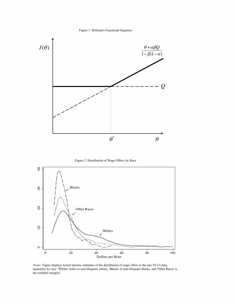
Figure 2: Distribution of Wage Offers, by Race

Notes: Figure displays kernel density estimates of the distribution of wage offers in the raw NJ UI data, separately by race. 'Whites' refers to non-Hispanic whites, 'Blacks' to non-Hispanic blacks, and 'Other Races' is the residual category.

Figure 1: Bellman's Functional Equation

!

J(! )

Q

! *

! +"#Q1!#(1!")

Blacks

Whites

Other Races

0.0

2.0

4.0

6.0

8

0 20 40 60 80 100Dollars per Hour

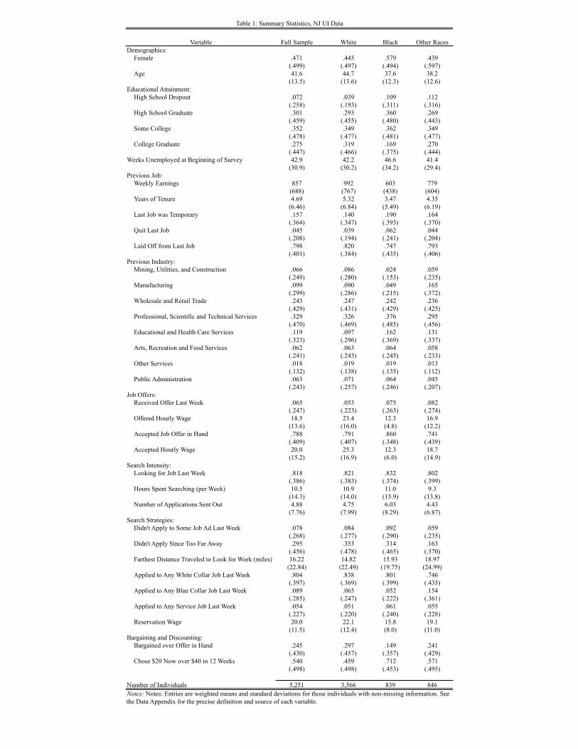
Variable Full Sample White Black Other RacesDemographics:

Female .471 .445 .579 .439(.499) (.497) (.494) (.597)

Age 41.6 44.7 37.6 38.2(13.5) (13.6) (12.3) (12.6)

Educational Attainment:High School Dropout .072 .039 .109 .112

(.258) (.193) (.311) (.316)High School Graduate .301 .293 .360 .269 (.459) (.455) (.480) (.443)Some College .352 .349 .362 .349

(.478) (.477) (.481) (.477)College Graduate .275 .319 .169 .270

(.447) (.466) (.375) (.444)Weeks Unemployed at Beginning of Survey 42.9 42.2 46.6 41.4

(30.9) (30.2) (34.2) (29.4)Previous Job:

Weekly Earnings 857 992 603 779(688) (767) (438) (604)

Years of Tenure 4.69 5.32 3.47 4.35(6.46) (6.84) (5.49) (6.19)

Last Job was Temporary .157 .140 .190 .164(.364) (.347) (.393) (.370)

Quit Last Job .045 .039 .062 .044(.208) (.194) (.241) (.204)

Laid Off from Last Job .798 .820 .747 .793(.401) (.384) (.435) (.406)

Previous Industry:Mining, Utilities, and Construction .066 .086 .024 .059

(.249) (.280) (.153) (.235)Manufacturing .099 .090 .049 .165

(.299) (.286) (.215) (.372)Wholesale and Retail Trade .243 .247 .242 .236

(.429) (.431) (.429) (.425)Professional, Scientific and Technical Services .329 .326 .376 .295

(.470) (.469) (.485) (.456)Educational and Health Care Services .119 .097 .162 .131

(.323) (.296) (.369) (.337)Arts, Recreation and Food Services .062 .063 .064 .058

(.241) (.243) (.245) (.233)Other Services .018 .019 .019 .013

(.132) (.138) (.135) (.112)Public Administration .063 .071 .064 .045

(.243) (.257) (.246) (.207)Job Offers:

Received Offer Last Week .065 .053 .075 .082(.247) (.223) (.263) (.274)

Offered Hourly Wage 18.5 23.4 12.3 16.9(13.6) (16.0) (4.8) (12.2)

Accepted Job Offer in Hand .788 .791 .860 .741(.409) (.407) (.348) (.439)

Accepted Hourly Wage 20.0 25.3 12.3 18.7(15.2) (16.9) (6.0) (14.9)

Search Intensity:Looking for Job Last Week .818 .821 .832 .802

(.386) (.383) (.374) (.399)Hours Spent Searching (per Week) 10.5 10.9 11.0 9.3

(14.3) (14.0) (15.9) (13.8)Number of Applications Sent Out 4.88 4.75 6.03 4.43

(7.76) (7.99) (8.29) (6.87)Search Strategies:

Didn't Apply to Some Job Ad Last Week .078 .084 .092 .059(.268) (.277) (.290) (.235)

Didn't Apply Since Too Far Away .295 .353 .314 .163(.456) (.478) (.465) (.370)

Farthest Distance Traveled to Look for Work (miles) 16.22 14.82 15.93 18.97(22.84) (22.49) (19.75) (24.99)

Applied to Any White Collar Job Last Week .804 .838 .801 .746(.397) (.369) (.399) (.435)

Applied to Any Blue Collar Job Last Week .089 .065 .052 .154(.285) (.247) (.222) (.361)

Applied to Any Service Job Last Week .054 .051 .061 .055(.227) (.220) (.240) (.228)

Reservation Wage 20.0 22.1 15.8 19.1(11.5) (12.4) (8.0) (11.0)

Bargaining and Discounting:Bargained over Offer in Hand .245 .297 .149 .241

(.430) (.457) (.357) (.429)Chose $20 Now over $40 in 12 Weeks .540 .459 .712 .571

(.498) (.498) (.453) (.495)

Number of Individuals 5,251 3,566 839 846

Table 1: Summary Statistics, NJ UI Data

Notes: Notes: Entries are weighted means and standard deviations for those individuals with non-missing information. See the Data Appendix for the precise definition and source of each variable.

Independent Variable (1) (2) (3) (4) (5)Black -.404 -.286 -.169 -.165 -.160

(.059) (.061) (.056) (.057) (.060)Other Races -.243 -.233 -.170 -.173 -.201

(.085) (.072) (.063) (.065) (.063)Female -.162 -.248 -.101 -.096 -.114

(.064) (.062) (.051) (.050) (.048)Age .041 .042 .003 .007 .002

(.016) (.016) (.015) (.015) (.014)Age Squared (÷100) -.040 -.042 -.000 -.004 .001

(.020) (.020) (.019) (.018) (.017)High School Graduate -.074 -.124 -.142 -.086

(.120) (.102) (.108) (.099)Some College .251 .060 .041 .084

(.122) (.102) (.107) (.094)College Graduate .451 .164 .150 .206

(.129) (.101) (.106) (.098)Log Previous Weekly Earnings .416 .408 .417

(.052) (.051) (.051)Weeks Unemployed -.005 -.006

(.003) (.003)Weeks Unemployed Squared (÷100) .003 .003

(.002) (.002)Quit Last Job .019 -.006

(.112) (.105)Last Job was Temporary .054 .044

(.068) (.069)Constant 2.068 1.840 -.005 .093 .146

(.321) (.342) (.368) (.384) (.390)Previous Industry Fixed Effects No No No No YesR-Squared .192 .320 .479 .489 .512Number of Observations 1,194 1,194 1,194 1,194 1,194

Table 2: Racial Differences in Wage Offers, NJ UI Data

Notes: Entries are coefficients and standard errors from estimating the empirical model by weighted least squares. Heteroskedasticity robust standard errors are clustered by individual and reported in parentheses. In addition to the variables shown in the table, indicator variables for missing values on each covariate are also included in the regressions. See the Data Appendix for the precise definition and source of each variable.

Log Offered Hourly Wage

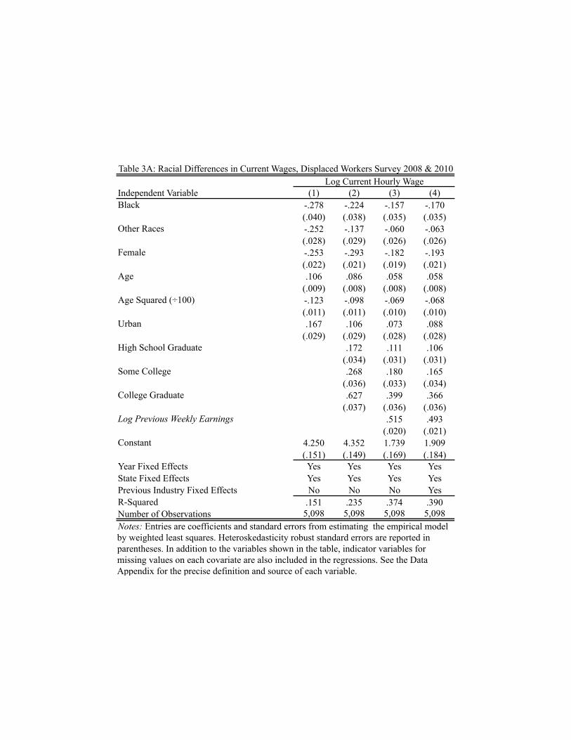
Independent Variable (1) (2) (3) (4)Black -.278 -.224 -.157 -.170

(.040) (.038) (.035) (.035)Other Races -.252 -.137 -.060 -.063

(.028) (.029) (.026) (.026)Female -.253 -.293 -.182 -.193

(.022) (.021) (.019) (.021)Age .106 .086 .058 .058

(.009) (.008) (.008) (.008)Age Squared (÷100) -.123 -.098 -.069 -.068

(.011) (.011) (.010) (.010)Urban .167 .106 .073 .088

(.029) (.029) (.028) (.028)High School Graduate .172 .111 .106

(.034) (.031) (.031)Some College .268 .180 .165

(.036) (.033) (.034)College Graduate .627 .399 .366

(.037) (.036) (.036)Log Previous Weekly Earnings .515 .493

(.020) (.021)Constant 4.250 4.352 1.739 1.909

(.151) (.149) (.169) (.184)Year Fixed Effects Yes Yes Yes YesState Fixed Effects Yes Yes Yes YesPrevious Industry Fixed Effects No No No YesR-Squared .151 .235 .374 .390Number of Observations 5,098 5,098 5,098 5,098

Table 3A: Racial Differences in Current Wages, Displaced Workers Survey 2008 & 2010Log Current Hourly Wage

Notes: Entries are coefficients and standard errors from estimating the empirical model by weighted least squares. Heteroskedasticity robust standard errors are reported in parentheses. In addition to the variables shown in the table, indicator variables for missing values on each covariate are also included in the regressions. See the Data Appendix for the precise definition and source of each variable.

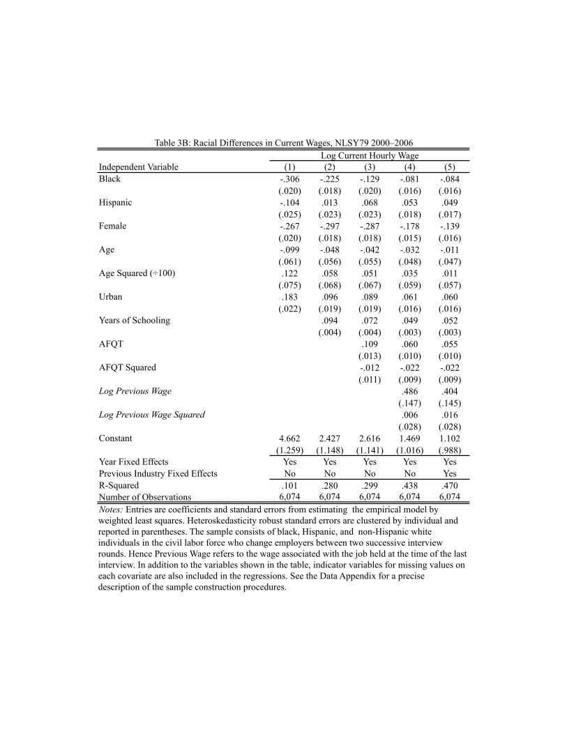
Independent Variable (1) (2) (3) (4) (5)Black -.306 -.225 -.129 -.081 -.084

(.020) (.018) (.020) (.016) (.016)Hispanic -.104 .013 .068 .053 .049

(.025) (.023) (.023) (.018) (.017)Female -.267 -.297 -.287 -.178 -.139

(.020) (.018) (.018) (.015) (.016)Age -.099 -.048 -.042 -.032 -.011

(.061) (.056) (.055) (.048) (.047)Age Squared (÷100) .122 .058 .051 .035 .011

(.075) (.068) (.067) (.059) (.057)Urban .183 .096 .089 .061 .060

(.022) (.019) (.019) (.016) (.016)Years of Schooling .094 .072 .049 .052

(.004) (.004) (.003) (.003)AFQT .109 .060 .055

(.013) (.010) (.010)AFQT Squared -.012 -.022 -.022

(.011) (.009) (.009)Log Previous Wage .486 .404

(.147) (.145)Log Previous Wage Squared .006 .016

(.028) (.028)Constant 4.662 2.427 2.616 1.469 1.102

(1.259) (1.148) (1.141) (1.016) (.988)Year Fixed Effects Yes Yes Yes Yes YesPrevious Industry Fixed Effects No No No No YesR-Squared .101 .280 .299 .438 .470Number of Observations 6,074 6,074 6,074 6,074 6,074

Table 3B: Racial Differences in Current Wages, NLSY79 2000–2006Log Current Hourly Wage

Notes: Entries are coefficients and standard errors from estimating the empirical model by weighted least squares. Heteroskedasticity robust standard errors are clustered by individual and reported in parentheses. The sample consists of black, Hispanic, and non-Hispanic white individuals in the civil labor force who change employers between two successive interview rounds. Hence Previous Wage refers to the wage associated with the job held at the time of the last interview. In addition to the variables shown in the table, indicator variables for missing values on each covariate are also included in the regressions. See the Data Appendix for a precise description of the sample construction procedures.

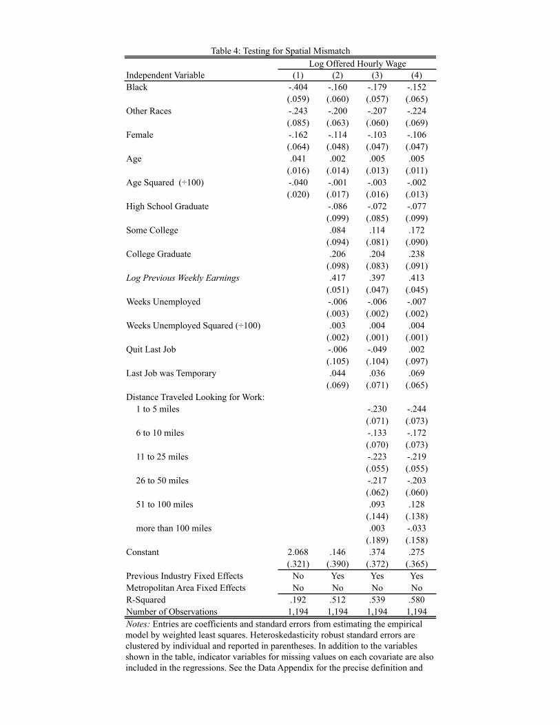
Independent Variable (1) (2) (3) (4)Black -.404 -.160 -.179 -.152

(.059) (.060) (.057) (.065)Other Races -.243 -.200 -.207 -.224

(.085) (.063) (.060) (.069)Female -.162 -.114 -.103 -.106

(.064) (.048) (.047) (.047)Age .041 .002 .005 .005

(.016) (.014) (.013) (.011)Age Squared (÷100) -.040 -.001 -.003 -.002

(.020) (.017) (.016) (.013)High School Graduate -.086 -.072 -.077

(.099) (.085) (.099)Some College .084 .114 .172

(.094) (.081) (.090)College Graduate .206 .204 .238

(.098) (.083) (.091)Log Previous Weekly Earnings .417 .397 .413

(.051) (.047) (.045)Weeks Unemployed -.006 -.006 -.007

(.003) (.002) (.002)Weeks Unemployed Squared (÷100) .003 .004 .004

(.002) (.001) (.001)Quit Last Job -.006 -.049 .002

(.105) (.104) (.097)Last Job was Temporary .044 .036 .069

(.069) (.071) (.065)Distance Traveled Looking for Work:

1 to 5 miles -.230 -.244(.071) (.073)

6 to 10 miles -.133 -.172(.070) (.073)

11 to 25 miles -.223 -.219(.055) (.055)

26 to 50 miles -.217 -.203(.062) (.060)

51 to 100 miles .093 .128(.144) (.138)

more than 100 miles .003 -.033(.189) (.158)

Constant 2.068 .146 .374 .275(.321) (.390) (.372) (.365)

Previous Industry Fixed Effects No Yes Yes YesMetropolitan Area Fixed Effects No No No NoR-Squared .192 .512 .539 .580Number of Observations 1,194 1,194 1,194 1,194

Table 4: Testing for Spatial MismatchLog Offered Hourly Wage

Notes: Entries are coefficients and standard errors from estimating the empirical model by weighted least squares. Heteroskedasticity robust standard errors are clustered by individual and reported in parentheses. In addition to the variables shown in the table, indicator variables for missing values on each covariate are also included in the regressions. See the Data Appendix for the precise definition and source of each variable.

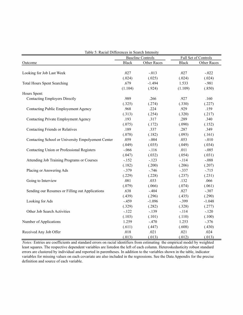
Outcome Black Other Races Black Other Races

Looking for Job Last Week .027 -.013 .027 -.022(.024) (.025) (.024) (.024)

Total Hours Spent Searching .679 -1.494 1.533 -.981(1.104) (.924) (1.109) (.850)

Hours Spent:Contacting Employers Directly .989 .266 .927 .160

(.325) (.274) (.330) (.227)Contacting Public Employement Agency .968 .224 .929 .159

(.313) (.254) (.320) (.217)Contacting Private Employment Agency .193 .317 .289 .340

(.075) (.172) (.090) (.152)Contacting Friends or Relatives .189 .337 .287 .349

(.078) (.182) (.093) (.161)Contacting School or University Empolyement Center .059 -.004 .053 -.010

(.049) (.035) (.049) (.034)Contacting Union or Professional Registers -.066 -.116 .011 -.085

(.047) (.032) (.054) (.031)Attending Job Training Programs or Courses -.152 -.123 -.114 -.088

(.182) (.200) (.206) (.207)Placing or Answering Ads -.379 -.746 -.337 -.715

(.229) (.228) (.237) (.231)Going to Interview .081 .033 .132 .066

(.079) (.066) (.074) (.061)Sending our Resumes or Filling out Applications .638 -.404 .827 -.307

(.439) (.296) (.435) (.290)Looking for Ads -.459 -1.096 -.399 -1.048

(.329) (.282) (.328) (.277)Other Job Search Activities -.122 -.139 -.114 -.120

(.103) (.101) (.110) (.100)Number of Applications 1.259 -.470 1.253 -.376

(.611) (.447) (.608) (.430)Received Any Job Offer .018 .021 .021 .024

(.013) (.013) (.012) (.013)

Table 5: Racial Differences in Search Intensity

Notes: Entries are coefficients and standard errors on racial identifiers from estimating the empirical model by weighted least squares. The respective dependent variables are listedon the left of each column. Heteroskedasticity robust standard errors are clustered by individual and reported in parentheses. In addition to the variables shown in the table, indicator variables for missing values on each covariate are also included in the regressions. See the Data Appendix for the precise definition and source of each variable.

Baseline Controls Full Set of Controls

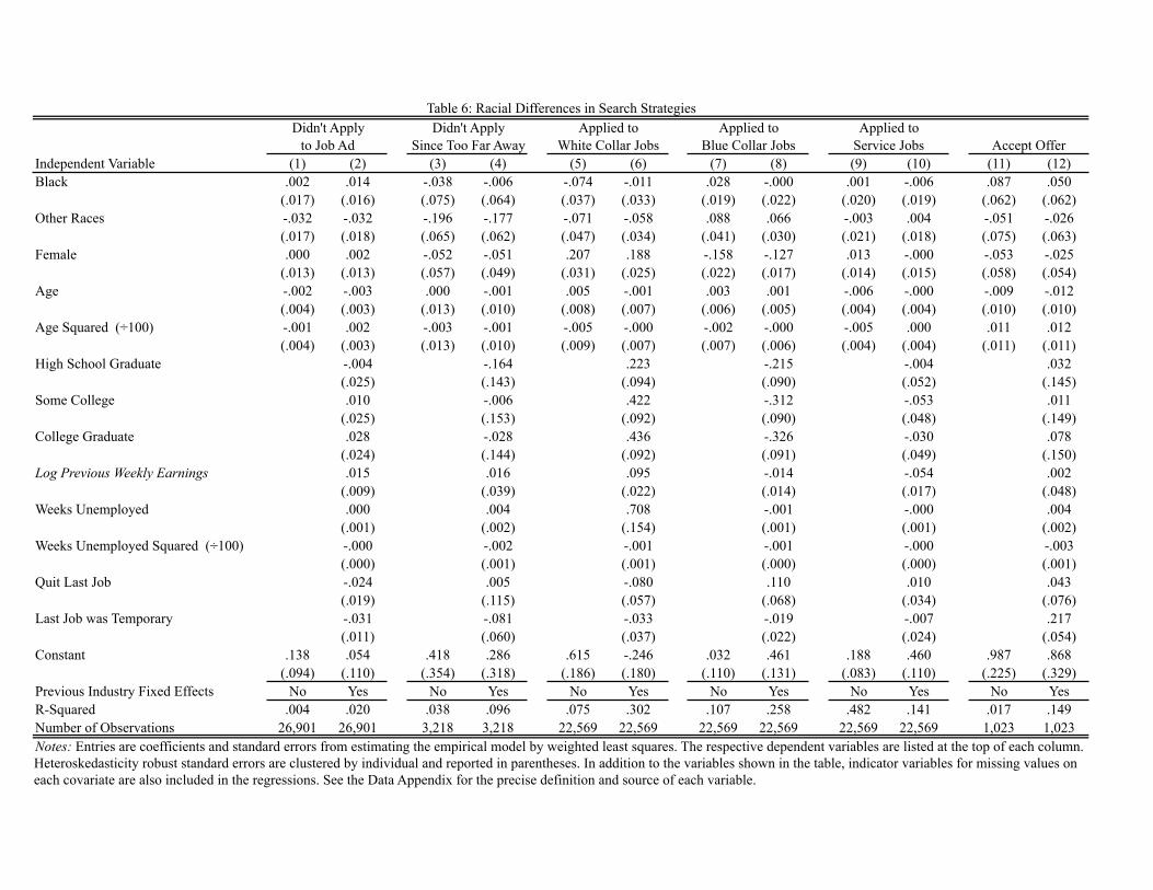
Independent Variable (1) (2) (3) (4) (5) (6) (7) (8) (9) (10) (11) (12)Black .002 .014 -.038 -.006 -.074 -.011 .028 -.000 .001 -.006 .087 .050

(.017) (.016) (.075) (.064) (.037) (.033) (.019) (.022) (.020) (.019) (.062) (.062)Other Races -.032 -.032 -.196 -.177 -.071 -.058 .088 .066 -.003 .004 -.051 -.026

(.017) (.018) (.065) (.062) (.047) (.034) (.041) (.030) (.021) (.018) (.075) (.063)Female .000 .002 -.052 -.051 .207 .188 -.158 -.127 .013 -.000 -.053 -.025

(.013) (.013) (.057) (.049) (.031) (.025) (.022) (.017) (.014) (.015) (.058) (.054)Age -.002 -.003 .000 -.001 .005 -.001 .003 .001 -.006 -.000 -.009 -.012

(.004) (.003) (.013) (.010) (.008) (.007) (.006) (.005) (.004) (.004) (.010) (.010)Age Squared (÷100) -.001 .002 -.003 -.001 -.005 -.000 -.002 -.000 -.005 .000 .011 .012

(.004) (.003) (.013) (.010) (.009) (.007) (.007) (.006) (.004) (.004) (.011) (.011)High School Graduate -.004 -.164 .223 -.215 -.004 .032

(.025) (.143) (.094) (.090) (.052) (.145)Some College .010 -.006 .422 -.312 -.053 .011

(.025) (.153) (.092) (.090) (.048) (.149)College Graduate .028 -.028 .436 -.326 -.030 .078

(.024) (.144) (.092) (.091) (.049) (.150)Log Previous Weekly Earnings .015 .016 .095 -.014 -.054 .002

(.009) (.039) (.022) (.014) (.017) (.048)Weeks Unemployed .000 .004 .708 -.001 -.000 .004

(.001) (.002) (.154) (.001) (.001) (.002)Weeks Unemployed Squared (÷100) -.000 -.002 -.001 -.001 -.000 -.003

(.000) (.001) (.001) (.000) (.000) (.001)Quit Last Job -.024 .005 -.080 .110 .010 .043

(.019) (.115) (.057) (.068) (.034) (.076)Last Job was Temporary -.031 -.081 -.033 -.019 -.007 .217

(.011) (.060) (.037) (.022) (.024) (.054)Constant .138 .054 .418 .286 .615 -.246 .032 .461 .188 .460 .987 .868

(.094) (.110) (.354) (.318) (.186) (.180) (.110) (.131) (.083) (.110) (.225) (.329)Previous Industry Fixed Effects No Yes No Yes No Yes No Yes No Yes No YesR-Squared .004 .020 .038 .096 .075 .302 .107 .258 .482 .141 .017 .149Number of Observations 26,901 26,901 3,218 3,218 22,569 22,569 22,569 22,569 22,569 22,569 1,023 1,023

Blue Collar JobsApplied to Applied to

Table 6: Racial Differences in Search Strategies

Notes: Entries are coefficients and standard errors from estimating the empirical model by weighted least squares. The respective dependent variables are listed at the top of each column. Heteroskedasticity robust standard errors are clustered by individual and reported in parentheses. In addition to the variables shown in the table, indicator variables for missing values on each covariate are also included in the regressions. See the Data Appendix for the precise definition and source of each variable.

Accept OfferDidn't Apply

to Job Ad Since Too Far AwayDidn't Apply

White Collar JobsApplied to

Service Jobs

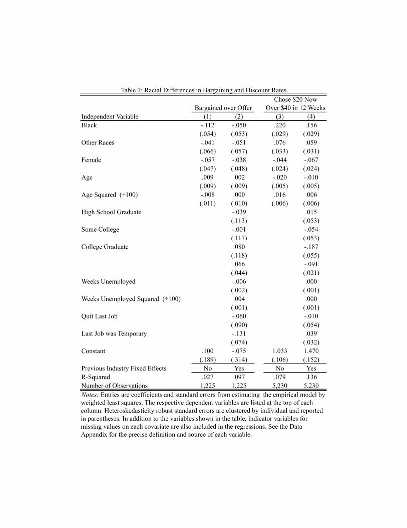
Independent Variable (1) (2) (3) (4)Black -.112 -.050 .220 .156

(.054) (.053) (.029) (.029)Other Races -.041 -.051 .076 .059

(.066) (.057) (.033) (.031)Female -.057 -.038 -.044 -.067

(.047) (.048) (.024) (.024)Age .009 .002 -.020 -.010

(.009) (.009) (.005) (.005)Age Squared (÷100) -.008 .000 .016 .006

(.011) (.010) (.006) (.006)High School Graduate -.039 .015

(.113) (.053)Some College -.001 -.054

(.117) (.053)College Graduate .080 -.187

(.118) (.055).066 -.091

(.044) (.021)Weeks Unemployed -.006 .000

(.002) (.001)Weeks Unemployed Squared (÷100) .004 .000

(.001) (.001)Quit Last Job -.060 -.010

(.090) (.054)Last Job was Temporary -.131 .039

(.074) (.032)Constant .100 -.075 1.033 1.470

(.189) (.314) (.106) (.152)Previous Industry Fixed Effects No Yes No YesR-Squared .027 .097 .079 .136Number of Observations 1,225 1,225 5,230 5,230

Table 7: Racial Differences in Bargaining and Discount Rates

Notes: Entries are coefficients and standard errors from estimating the empirical model by weighted least squares. The respective dependent variables are listed at the top of each column. Heteroskedasticity robust standard errors are clustered by individual and reported in parentheses. In addition to the variables shown in the table, indicator variables for missing values on each covariate are also included in the regressions. See the Data Appendix for the precise definition and source of each variable.

Bargained over OfferChose $20 Now

Over $40 in 12 Weeks

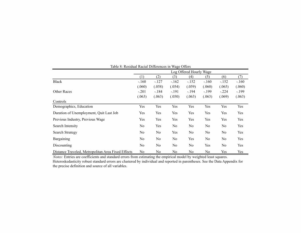
(1) (2) (3) (4) (5) (6) (7)Black -.160 -.127 -.162 -.152 -.160 -.152 -.160

(.060) (.058) (.054) (.059) (.060) (.065) (.060)Other Races -.201 -.184 -.191 -.194 -.199 -.224 -.199

(.063) (.063) (.050) (.063) (.063) (.069) (.063)ControlsDemographics, Education Yes Yes Yes Yes Yes Yes Yes

Duration of Unemployment, Quit Last Job Yes Yes Yes Yes Yes Yes Yes

Previous Industry, Previous Wage Yes Yes Yes Yes Yes Yes Yes

Search Intensity No Yes No No No No Yes

Search Strategy No No Yes No No No Yes

Bargaining No No No Yes No No Yes

Discounting No No No No Yes No Yes

Distance Traveled, Metropolitan Area Fixed Effects No No No No No Yes Yes

Table 8: Residual Racial Differences in Wage OffersLog Offered Hourly Wage

Notes: Entries are coefficients and standard errors from estimating the empirical model by weighted least squares. Heteroskedasticity robust standard errors are clustered by individual and reported in parentheses. See the Data Appendix for the precise definition and source of all variables.

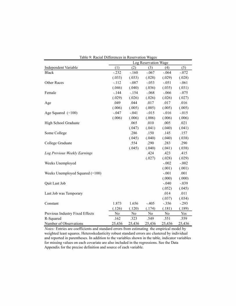
Independent Variable (1) (2) (3) (4) (5)Black -.232 -.160 -.067 -.064 -.072

(.033) (.033) (.028) (.029) (.028)Other Races -.112 -.087 -.053 -.051 -.061

(.046) (.040) (.036) (.035) (.031)Female -.144 -.154 -.068 -.066 -.075

(.029) (.026) (.026) (.026) (.027)Age .049 .044 .017 .017 .016

(.006) (.005) (.005) (.005) (.005)Age Squared (÷100) -.047 -.041 -.015 -.016 -.015

(.006) (.006) (.006) (.006) (.006)High School Graduate .065 .010 .005 .021

(.047) (.041) (.040) (.041)Some College .286 .150 .145 .157

(.045) (.040) (.040) (.038)College Graduate .554 .290 .283 .290

(.045) (.040) (.041) (.038)Log Previous Weekly Earnings .424 .423 .415

(.027) (.028) (.029)Weeks Unemployed -.002 -.002

(.001) (.001)Weeks Unemployed Squared (÷100) -.001 .001

(.000) (.000)Quit Last Job -.040 -.039

(.052) (.045)Last Job was Temporary .014 .011

(.037) (.034)Constant 1.873 1.656 -.405 -.356 -.293

(.126) (.120) (.174) (.181) (.189)Previous Industry Fixed Effects No No No No YesR-Squared .162 .323 .549 .551 .559Number of Observations 25,436 25,436 25,436 25,436 25,436

Table 9: Racial Differences in Reservation Wages

Notes: Entries are coefficients and standard errors from estimating the empirical model by weighted least squares. Heteroskedasticity robust standard errors are clustered by individual and reported in parentheses. In addition to the variables shown in the table, indicator variables for missing values on each covariate are also included in the regressions. See the Data Appendix for the precise definition and source of each variable.

Log Reservation Wage

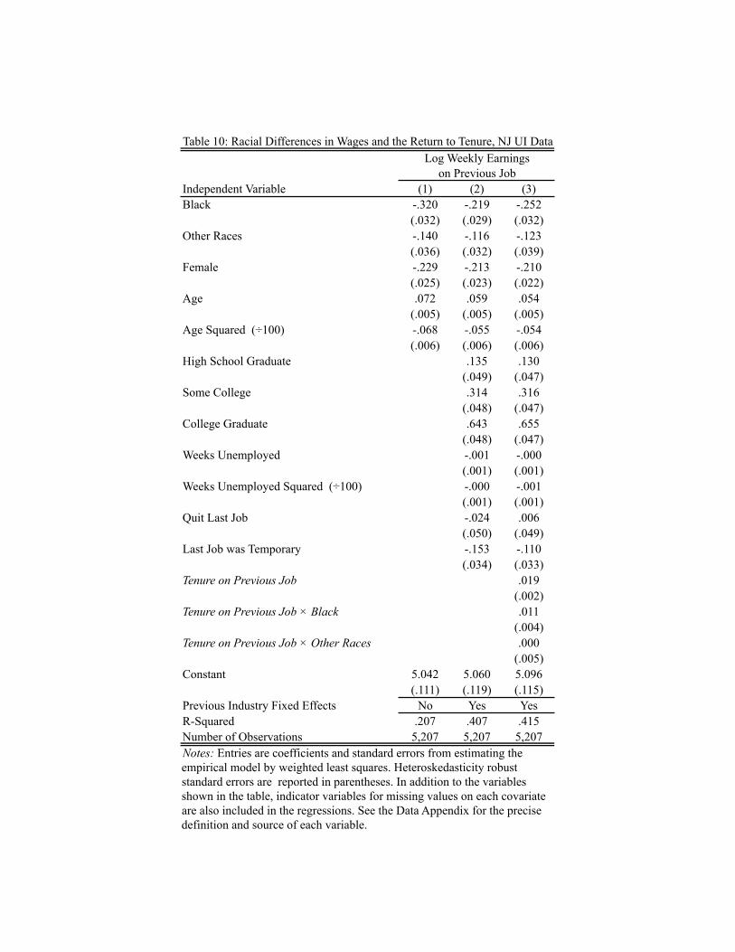
Independent Variable (1) (2) (3)Black -.320 -.219 -.252

(.032) (.029) (.032)Other Races -.140 -.116 -.123

(.036) (.032) (.039)Female -.229 -.213 -.210

(.025) (.023) (.022)Age .072 .059 .054

(.005) (.005) (.005)Age Squared (÷100) -.068 -.055 -.054

(.006) (.006) (.006)High School Graduate .135 .130

(.049) (.047)Some College .314 .316

(.048) (.047)College Graduate .643 .655

(.048) (.047)Weeks Unemployed -.001 -.000

(.001) (.001)Weeks Unemployed Squared (÷100) -.000 -.001

(.001) (.001)Quit Last Job -.024 .006

(.050) (.049)Last Job was Temporary -.153 -.110

(.034) (.033)Tenure on Previous Job .019

(.002)Tenure on Previous Job ! Black .011

(.004)Tenure on Previous Job ! Other Races .000

(.005)Constant 5.042 5.060 5.096

(.111) (.119) (.115)Previous Industry Fixed Effects No Yes YesR-Squared .207 .407 .415Number of Observations 5,207 5,207 5,207

Table 10: Racial Differences in Wages and the Return to Tenure, NJ UI Data

Notes: Entries are coefficients and standard errors from estimating the empirical model by weighted least squares. Heteroskedasticity robust standard errors are reported in parentheses. In addition to the variables shown in the table, indicator variables for missing values on each covariate are also included in the regressions. See the Data Appendix for the precise definition and source of each variable.

Log Weekly Earningson Previous Job

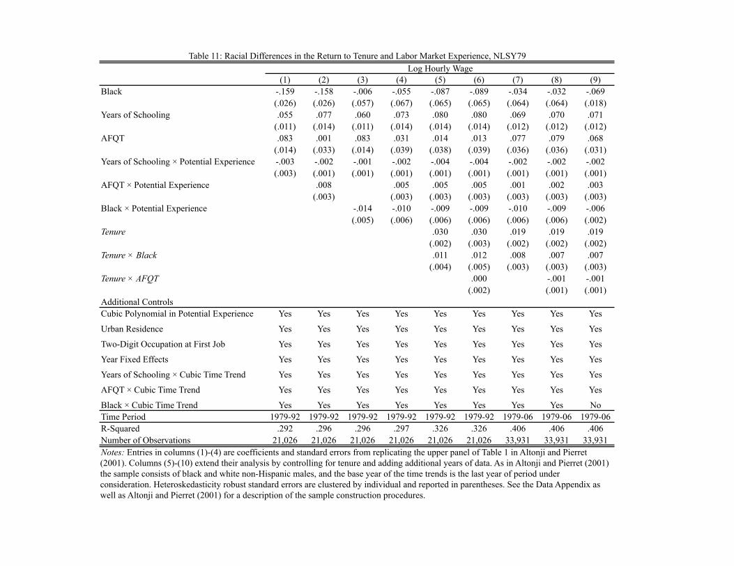
(1) (2) (3) (4) (5) (6) (7) (8) (9)Black -.159 -.158 -.006 -.055 -.087 -.089 -.034 -.032 -.069

(.026) (.026) (.057) (.067) (.065) (.065) (.064) (.064) (.018)Years of Schooling .055 .077 .060 .073 .080 .080 .069 .070 .071

(.011) (.014) (.011) (.014) (.014) (.014) (.012) (.012) (.012)AFQT .083 .001 .083 .031 .014 .013 .077 .079 .068

(.014) (.033) (.014) (.039) (.038) (.039) (.036) (.036) (.031)Years of Schooling ! Potential Experience -.003 -.002 -.001 -.002 -.004 -.004 -.002 -.002 -.002

(.003) (.001) (.001) (.001) (.001) (.001) (.001) (.001) (.001)AFQT ! Potential Experience .008 .005 .005 .005 .001 .002 .003

(.003) (.003) (.003) (.003) (.003) (.003) (.003)Black ! Potential Experience -.014 -.010 -.009 -.009 -.010 -.009 -.006

(.005) (.006) (.006) (.006) (.006) (.006) (.002)Tenure .030 .030 .019 .019 .019

(.002) (.003) (.002) (.002) (.002)Tenure ! Black .011 .012 .008 .007 .007

(.004) (.005) (.003) (.003) (.003)Tenure ! AFQT .000 -.001 -.001

(.002) (.001) (.001)Additional ControlsCubic Polynomial in Potential Experience Yes Yes Yes Yes Yes Yes Yes Yes Yes

Urban Residence Yes Yes Yes Yes Yes Yes Yes Yes Yes

Two-Digit Occupation at First Job Yes Yes Yes Yes Yes Yes Yes Yes Yes

Year Fixed Effects Yes Yes Yes Yes Yes Yes Yes Yes Yes

Years of Schooling ! Cubic Time Trend Yes Yes Yes Yes Yes Yes Yes Yes Yes

AFQT ! Cubic Time Trend Yes Yes Yes Yes Yes Yes Yes Yes Yes

Black ! Cubic Time Trend Yes Yes Yes Yes Yes Yes Yes Yes NoTime Period 1979-92 1979-92 1979-92 1979-92 1979-92 1979-92 1979-06 1979-06 1979-06R-Squared .292 .296 .296 .297 .326 .326 .406 .406 .406Number of Observations 21,026 21,026 21,026 21,026 21,026 21,026 33,931 33,931 33,931

Table 11: Racial Differences in the Return to Tenure and Labor Market Experience, NLSY79Log Hourly Wage

Notes: Entries in columns (1)-(4) are coefficients and standard errors from replicating the upper panel of Table 1 in Altonji and Pierret (2001). Columns (5)-(10) extend their analysis by controlling for tenure and adding additional years of data. As in Altonji and Pierret (2001) the sample consists of black and white non-Hispanic males, and the base year of the time trends is the last year of period under consideration. Heteroskedasticity robust standard errors are clustered by individual and reported in parentheses. See the Data Appendix as well as Altonji and Pierret (2001) for a description of the sample construction procedures.

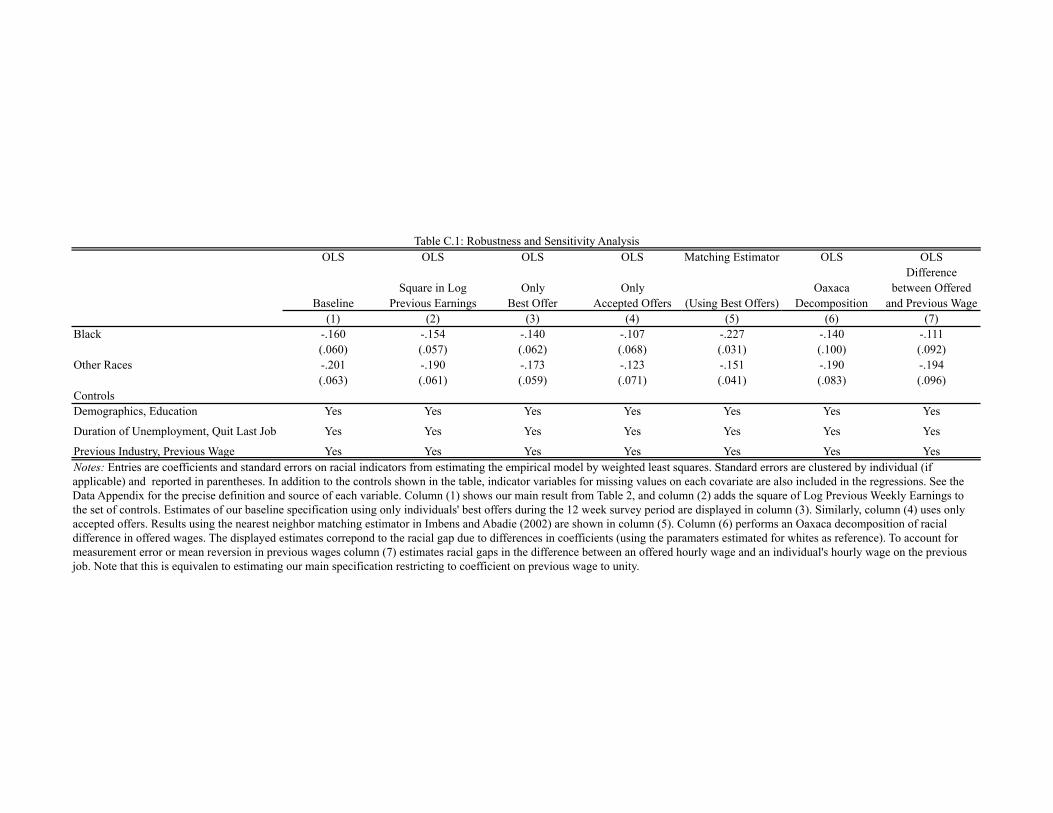
OLS OLS OLS OLS Matching Estimator OLS OLSDifference

Square in Log Only Only Oaxaca between OfferedBaseline Previous Earnings Best Offer Accepted Offers (Using Best Offers) Decomposition and Previous Wage

(1) (2) (3) (4) (5) (6) (7)Black -.160 -.154 -.140 -.107 -.227 -.140 -.111

(.060) (.057) (.062) (.068) (.031) (.100) (.092)Other Races -.201 -.190 -.173 -.123 -.151 -.190 -.194

(.063) (.061) (.059) (.071) (.041) (.083) (.096)ControlsDemographics, Education Yes Yes Yes Yes Yes Yes Yes

Duration of Unemployment, Quit Last Job Yes Yes Yes Yes Yes Yes Yes

Previous Industry, Previous Wage Yes Yes Yes Yes Yes Yes Yes

Table C.1: Robustness and Sensitivity Analysis

Notes: Entries are coefficients and standard errors on racial indicators from estimating the empirical model by weighted least squares. Standard errors are clustered by individual (if applicable) and reported in parentheses. In addition to the controls shown in the table, indicator variables for missing values on each covariate are also included in the regressions. See the Data Appendix for the precise definition and source of each variable. Column (1) shows our main result from Table 2, and column (2) adds the square of Log Previous Weekly Earnings to the set of controls. Estimates of our baseline specification using only individuals' best offers during the 12 week survey period are displayed in column (3). Similarly, column (4) uses only accepted offers. Results using the nearest neighbor matching estimator in Imbens and Abadie (2002) are shown in column (5). Column (6) performs an Oaxaca decomposition of racial difference in offered wages. The displayed estimates correpond to the racial gap due to differences in coefficients (using the paramaters estimated for whites as reference). To account for measurement error or mean reversion in previous wages column (7) estimates racial gaps in the difference between an offered hourly wage and an individual's hourly wage on the previous job. Note that this is equivalen to estimating our main specification restricting to coefficient on previous wage to unity.

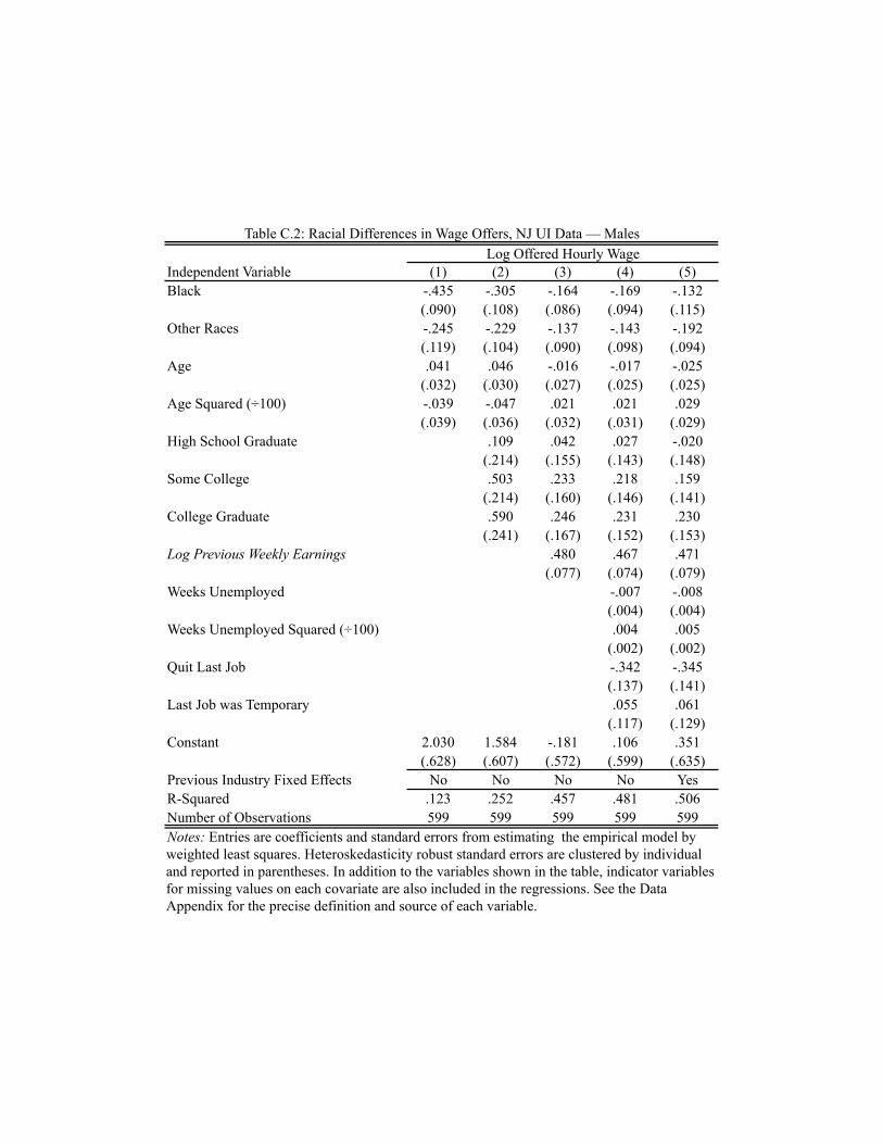
Independent Variable (1) (2) (3) (4) (5)Black -.435 -.305 -.164 -.169 -.132

(.090) (.108) (.086) (.094) (.115)Other Races -.245 -.229 -.137 -.143 -.192

(.119) (.104) (.090) (.098) (.094)Age .041 .046 -.016 -.017 -.025

(.032) (.030) (.027) (.025) (.025)Age Squared (÷100) -.039 -.047 .021 .021 .029

(.039) (.036) (.032) (.031) (.029)High School Graduate .109 .042 .027 -.020

(.214) (.155) (.143) (.148)Some College .503 .233 .218 .159

(.214) (.160) (.146) (.141)College Graduate .590 .246 .231 .230

(.241) (.167) (.152) (.153)Log Previous Weekly Earnings .480 .467 .471

(.077) (.074) (.079)Weeks Unemployed -.007 -.008

(.004) (.004)Weeks Unemployed Squared (÷100) .004 .005

(.002) (.002)Quit Last Job -.342 -.345

(.137) (.141)Last Job was Temporary .055 .061

(.117) (.129)Constant 2.030 1.584 -.181 .106 .351

(.628) (.607) (.572) (.599) (.635)Previous Industry Fixed Effects No No No No YesR-Squared .123 .252 .457 .481 .506Number of Observations 599 599 599 599 599

Table C.2: Racial Differences in Wage Offers, NJ UI Data — MalesLog Offered Hourly Wage

Notes: Entries are coefficients and standard errors from estimating the empirical model by weighted least squares. Heteroskedasticity robust standard errors are clustered by individual and reported in parentheses. In addition to the variables shown in the table, indicator variables for missing values on each covariate are also included in the regressions. See the Data Appendix for the precise definition and source of each variable.

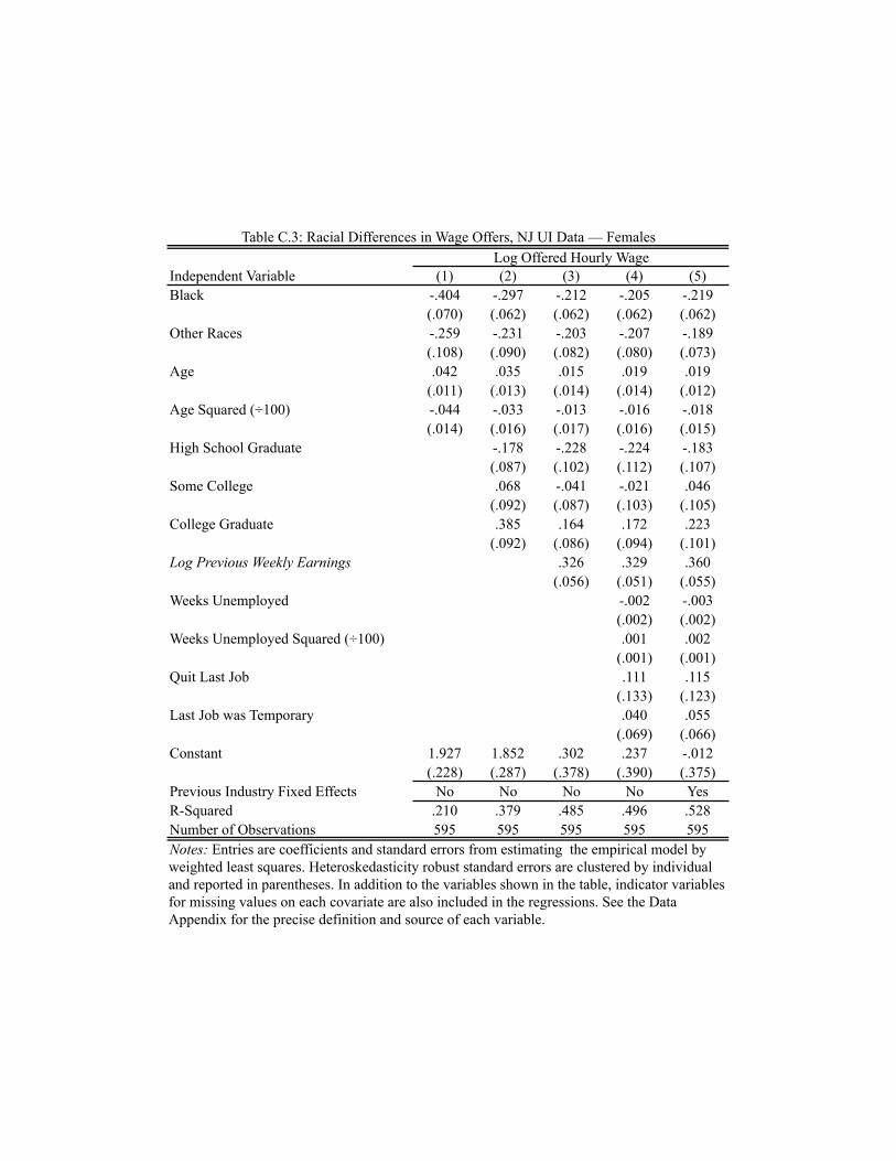
Independent Variable (1) (2) (3) (4) (5)Black -.404 -.297 -.212 -.205 -.219

(.070) (.062) (.062) (.062) (.062)Other Races -.259 -.231 -.203 -.207 -.189

(.108) (.090) (.082) (.080) (.073)Age .042 .035 .015 .019 .019

(.011) (.013) (.014) (.014) (.012)Age Squared (÷100) -.044 -.033 -.013 -.016 -.018

(.014) (.016) (.017) (.016) (.015)High School Graduate -.178 -.228 -.224 -.183

(.087) (.102) (.112) (.107)Some College .068 -.041 -.021 .046

(.092) (.087) (.103) (.105)College Graduate .385 .164 .172 .223

(.092) (.086) (.094) (.101)Log Previous Weekly Earnings .326 .329 .360

(.056) (.051) (.055)Weeks Unemployed -.002 -.003

(.002) (.002)Weeks Unemployed Squared (÷100) .001 .002

(.001) (.001)Quit Last Job .111 .115

(.133) (.123)Last Job was Temporary .040 .055

(.069) (.066)Constant 1.927 1.852 .302 .237 -.012

(.228) (.287) (.378) (.390) (.375)Previous Industry Fixed Effects No No No No YesR-Squared .210 .379 .485 .496 .528Number of Observations 595 595 595 595 595

Table C.3: Racial Differences in Wage Offers, NJ UI Data — FemalesLog Offered Hourly Wage

Notes: Entries are coefficients and standard errors from estimating the empirical model by weighted least squares. Heteroskedasticity robust standard errors are clustered by individual and reported in parentheses. In addition to the variables shown in the table, indicator variables for missing values on each covariate are also included in the regressions. See the Data Appendix for the precise definition and source of each variable.

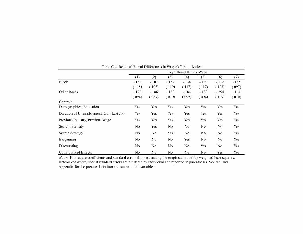
(1) (2) (3) (4) (5) (6) (7)Black -.132 -.107 -.167 -.138 -.139 -.112 -.185

(.115) (.105) (.119) (.117) (.117) (.103) (.097)Other Races -.192 -.186 -.150 -.184 -.188 -.254 -.164

(.094) (.087) (.079) (.095) (.094) (.109) (.070)ControlsDemographics, Education Yes Yes Yes Yes Yes Yes Yes

Duration of Unemployment, Quit Last Job Yes Yes Yes Yes Yes Yes Yes

Previous Industry, Previous Wage Yes Yes Yes Yes Yes Yes Yes

Search Intensity No Yes No No No No Yes

Search Strategy No No Yes No No No Yes

Bargaining No No No Yes No No Yes

Discounting No No No No Yes No Yes

County Fixed Effects No No No No No Yes Yes

Table C.4: Residual Racial Differences in Wage Offers — MalesLog Offered Hourly Wage

Notes: Entries are coefficients and standard errors from estimating the empirical model by weighted least squares. Heteroskedasticity robust standard errors are clustered by individual and reported in parentheses. See the Data Appendix for the precise definition and source of all variables.

(1) (2) (3) (4) (5) (6) (7)Black -.219 -.189 -.219 -.203 -.218 -.155 -.130

(.062) (.063) (.053) (.059) (.063) (.061) (.052)Other Races -.189 -.161 -.197 -.192 -.189 -.176 -.162

(.073) (.072) (.049) (.071) (.074) (.065) (.055)ControlsDemographics, Education Yes Yes Yes Yes Yes Yes Yes

Duration of Unemployment, Quit Last Job Yes Yes Yes Yes Yes Yes Yes

Previous Industry, Previous Wage Yes Yes Yes Yes Yes Yes Yes

Search Intensity No Yes No No No No Yes

Search Strategy No No Yes No No No Yes

Bargaining No No No Yes No No Yes

Discounting No No No No Yes No Yes

County Fixed Effects No No No No No Yes Yes

Table C.5: Residual Racial Differences in Wage Offers — FemalesLog Offered Hourly Wage

Notes: Entries are coefficients and standard errors from estimating the empirical model by weighted least squares. Heteroskedasticity robust standard errors are clustered by individual and reported in parentheses. See the Data Appendix for the precise definition and source of all variables.

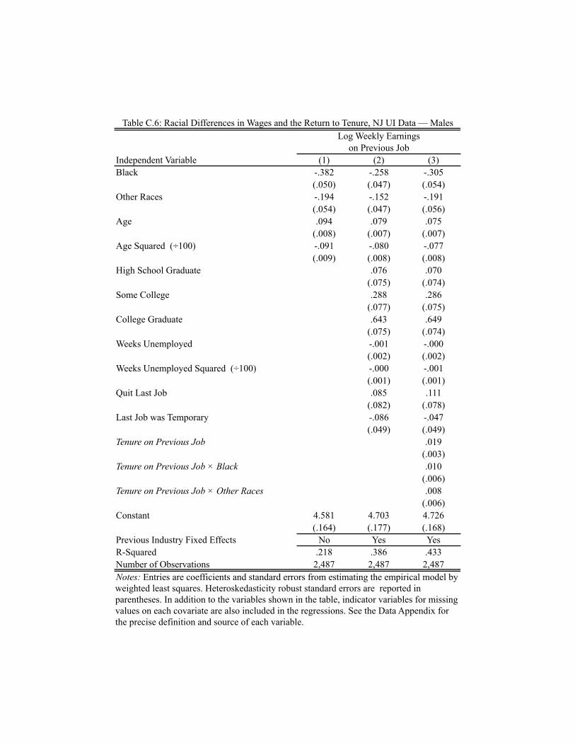
Independent Variable (1) (2) (3)Black -.382 -.258 -.305

(.050) (.047) (.054)Other Races -.194 -.152 -.191

(.054) (.047) (.056)Age .094 .079 .075

(.008) (.007) (.007)Age Squared (÷100) -.091 -.080 -.077

(.009) (.008) (.008)High School Graduate .076 .070

(.075) (.074)Some College .288 .286

(.077) (.075)College Graduate .643 .649

(.075) (.074)Weeks Unemployed -.001 -.000

(.002) (.002)Weeks Unemployed Squared (÷100) -.000 -.001

(.001) (.001)Quit Last Job .085 .111

(.082) (.078)Last Job was Temporary -.086 -.047

(.049) (.049)Tenure on Previous Job .019

(.003)Tenure on Previous Job ! Black .010

(.006)Tenure on Previous Job ! Other Races .008

(.006)Constant 4.581 4.703 4.726

(.164) (.177) (.168)Previous Industry Fixed Effects No Yes YesR-Squared .218 .386 .433Number of Observations 2,487 2,487 2,487

Table C.6: Racial Differences in Wages and the Return to Tenure, NJ UI Data — MalesLog Weekly Earnings

on Previous Job

Notes: Entries are coefficients and standard errors from estimating the empirical model by weighted least squares. Heteroskedasticity robust standard errors are reported in parentheses. In addition to the variables shown in the table, indicator variables for missing values on each covariate are also included in the regressions. See the Data Appendix for the precise definition and source of each variable.

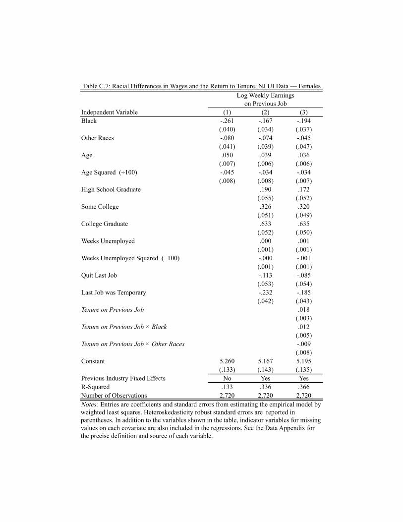
Independent Variable (1) (2) (3)Black -.261 -.167 -.194

(.040) (.034) (.037)Other Races -.080 -.074 -.045

(.041) (.039) (.047)Age .050 .039 .036

(.007) (.006) (.006)Age Squared (÷100) -.045 -.034 -.034

(.008) (.008) (.007)High School Graduate .190 .172

(.055) (.052)Some College .326 .320

(.051) (.049)College Graduate .633 .635

(.052) (.050)Weeks Unemployed .000 .001

(.001) (.001)Weeks Unemployed Squared (÷100) -.000 -.001

(.001) (.001)Quit Last Job -.113 -.085

(.053) (.054)Last Job was Temporary -.232 -.185

(.042) (.043)Tenure on Previous Job .018

(.003)Tenure on Previous Job ! Black .012

(.005)Tenure on Previous Job ! Other Races -.009

(.008)Constant 5.260 5.167 5.195

(.133) (.143) (.135)Previous Industry Fixed Effects No Yes YesR-Squared .133 .336 .366Number of Observations 2,720 2,720 2,720

Table C.7: Racial Differences in Wages and the Return to Tenure, NJ UI Data — FemalesLog Weekly Earnings

on Previous Job

Notes: Entries are coefficients and standard errors from estimating the empirical model by weighted least squares. Heteroskedasticity robust standard errors are reported in parentheses. In addition to the variables shown in the table, indicator variables for missing values on each covariate are also included in the regressions. See the Data Appendix for the precise definition and source of each variable.