1

Race to the Bottom:

Low Productivity, Market Power, and Lagging Wages

Lance Taylor and Özlem Ömer

Working Paper No. 80

August 8, 2018

ABSTRACT

“Dualism” in the structure of production across sectors of the US economy, employment by

sector, productivity levels and growth, real wages, and intersectoral terms-of trade increased

markedly between1990 and 2016. The discussion focuses on 16 sectors. Seven were “stagnant” -

- construction, education and health, other services, entertainment, accommodation and food,

business services, and transportation and warehousing. They had low productivity levels,

productivity growth rates hovering around zero, and low real wages. Their share of total

employment rose from 47% in 1990 to 61% in 2016. The other “dynamic” sectors had higher

and positively growing productivity while the terms-of- trade shifted against them. This

bifurcation between industries is discussed in terms of a simple model. Increasing duality and

secular stagnation are distinct possibilities.

* New School for Social Research. Support from the Institute for New Economic Thinking (INET) and

comments by Thomas Ferguson, Duncan Foley, Codrina Rada, and Servaas Storm are gratefully

acknowledged.

2

Keywords: economic dualism, industrial structure, productivity, low wages, employment

JEL Codes: D31, D33,E2, E12, E24, J40, L11

3

Output, employment, and income flows in the American economy became strikingly

more unbalanced over recent decades. In an old description from development economics, a

“dual economy” emerged, signaled by divergence between “stagnant” and “dynamic” sectors in

the structure of production, growing employment in stagnant industries, and rapidly rising

inequality in the functional and size distributions of income. Following INET-sponsored

research by Temin (2015) and Storm (2017), this paper takes a look at how the American dual

economy has evolved since 1990 when relevant data sets become available, and tries to assess

the major drivers.

The first topic is how production and distribution across industries or “sectors” of the

economy interact. Diagrams and numbers show the evolution of sectoral levels and growth of

real wages and labor “productivity,” a name for a widely discussed ratio,

Productivity = Real output ÷ Employment.

Productivity is an accounting relationship that links output, employment, and distribution. It is

tricky to apply. Complications are discussed below.1 We then turn to shifts in intersectoral

relative prices or the terms-of-trade between sectors. An explanatory framework is proposed,

drawing on insights from development economics and simple structuralist macro models.

In a common disaggregation, 16 producing sectors are used to illustrate structural change.

Compared to the others, seven sectors -- construction, education and health along with other

services (their two dots overlap), entertainment, accommodation and food, business services, and

transportation and warehousing -- have low levels of productivity. Their growth rates of

productivity and real wages lagged the rest. Their share of total employment rose from 47% in

1990 to 61% in 2016 while their share in wages went from 57% to 56% of the total. Despite their

high employment and output, they generated only 30% of total profits at the beginning of the

period and 23% at the end. Except for construction and transport, the shares of their own profits

in output declined.

The drastic fall in the share of wages relative to employment demonstrates visible wage

retardation. Their real output share fell from 48% to 41%. This shift of labor toward low wage,

low productivity jobs helps explain the striking increase of American income inequality.

1 In the jargon, real output is measured as double-deflated chain-indexed value-added, with data from the

US Bureau of Economic Analysis (BEA). Annual employment levels are provided by the Bureau of

Labor Statistics (BLS). The ins and outs of double deflation and chain indexing are set out in Moyer, et.

al. (2004) from the BEA.

4

Increasing imbalances

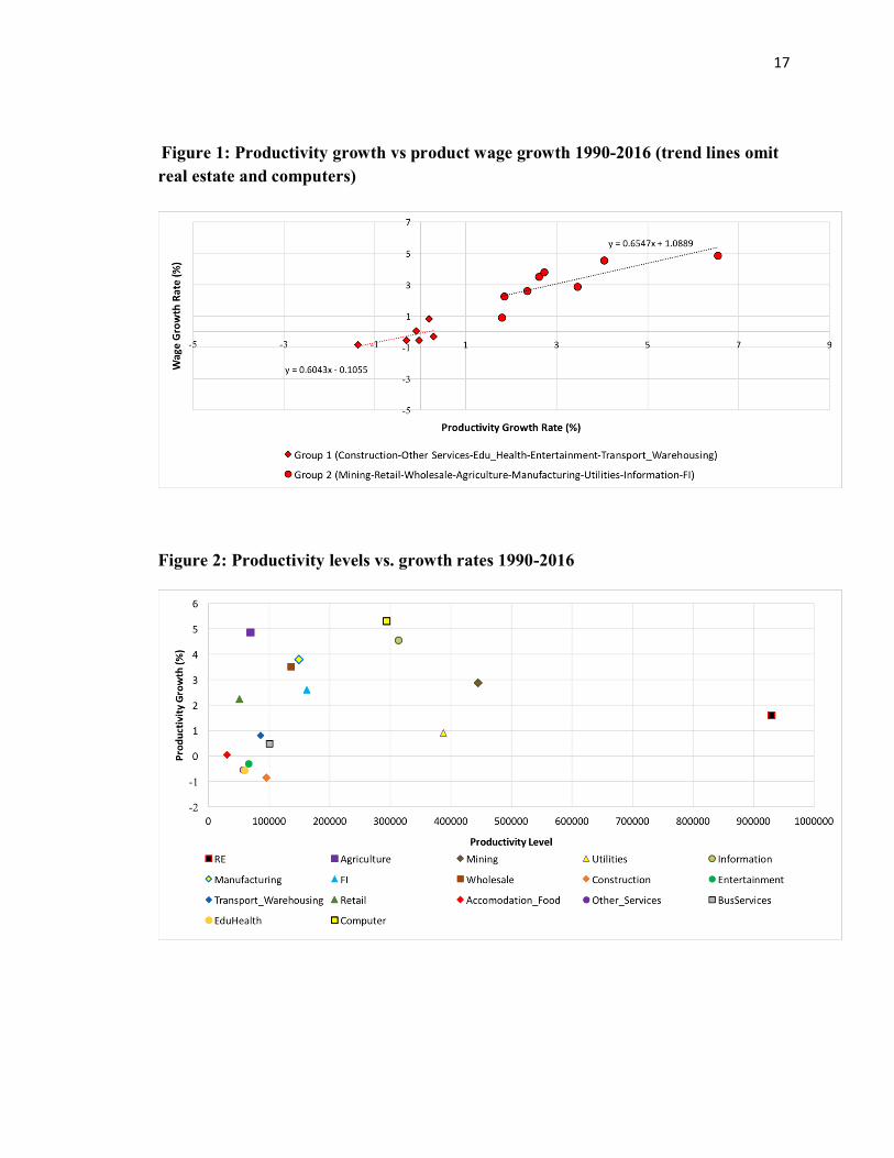
Figure 1 begins to tell the tale. Productivity growth rates 1990-2016 are displayed along

the horizontal axis. The seven lagging sectors had rates hovering around zero. Figure 2 shows

that these sectors along with retail trade and agriculture have productivity levels less than

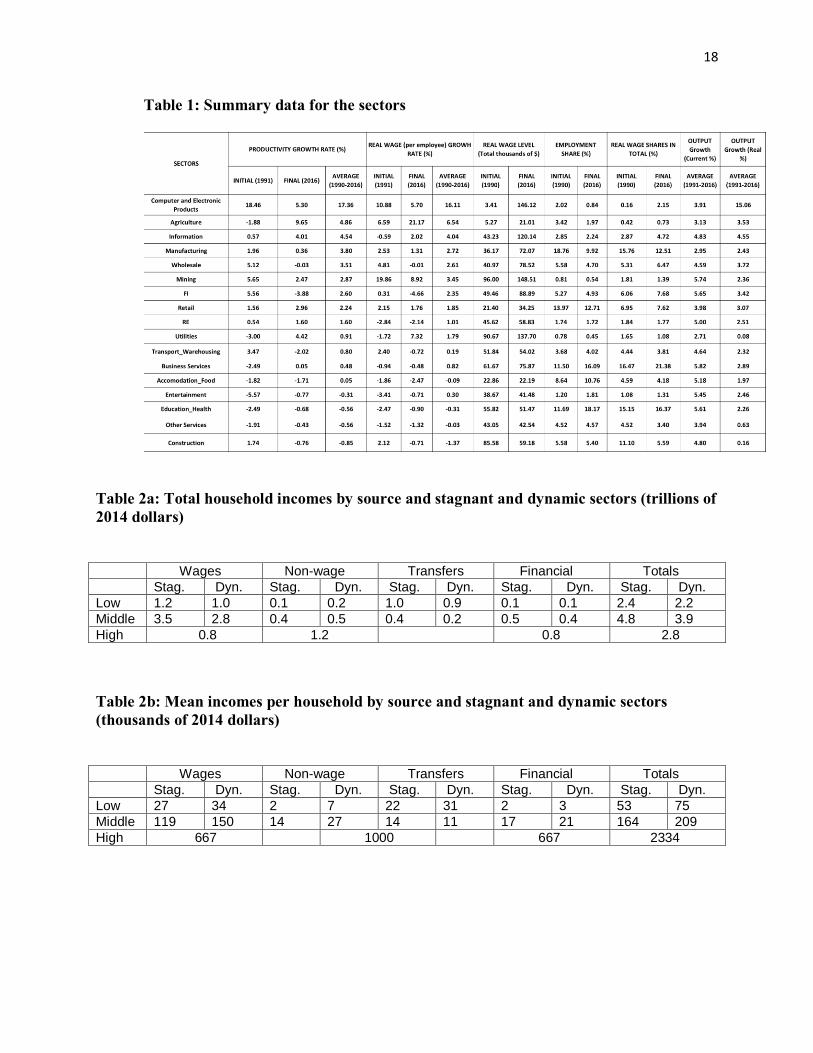
$100,000 per employed person per year (or roughly $55 per hour) in prices of 2009. Table 1

shows that the seven accounted for 46.8% of total employment in 1990 and 60.8% in 2016 – the

proportion of down-market jobs shot up.

Figure 1 here

Figure 2 here

Growth rates of real wages are plotted along the vertical axis in Figure 1.2 The rates for

the bottom sectors were dismal – all less than one percent per year and four negative (see Table

1). The slope of a trend line through the points (or the cross-sectional elasticity of wage growth

with respect to productivity growth) is 0.6. There was a substantial wage lag.

Table 1 here

The other sectors have higher productivity levels and/or growth. As noted above, retail

and agriculture have relatively low productivity but respectable growth. Utilities have high

productivity combined with slow growth. Finance and insurance (FI), manufacturing, wholesale,

information, and mining have solid performances on both counts. Real estate rental and leasing

has exceptionally high measured productivity. The real estate business collects fees and rents,

which flow into a profit share of value-added exceeding 90%, but it does not create many jobs. It

is basically an outlier. Computers and electronics comprise a sub-sector of manufacturing

included to illustrate the properties of a relatively small but leading branch of the economy.

2 The growth rates refer to “product wages” or the costs of labor to business. They were estimated as

current value wage shares of value-added times real labor productivity levels. The numbers are close to

independent estimates of real wages. To give an example in round numbers, the end-of-period wage share

in manufacturing was around 0.47. Productivity was $150 thousand, giving a wage of $70 thousand per

employee.

5

Ignoring real estate and computers, the trend line though the other sectors has a slope of

0.65. Bringing in the outliers gives a slope of 1.05. Either way, even the dynamic sectors

demonstrate a lag of overall wage payments behind productivity. The fact that labor payments

did not keep up with productivity across almost all sectors suggests that generalized wage

suppression rather than price increases due to business monopoly was the key factor in making

the income distribution become more unequal.3

A complicating factor enters in the form of an idea tracing at least back to Marx and

inserted into mainstream economics by Hicks (1932). Businesses can reduce labor costs by

cutting wages or increasing productivity. If they succeed with wage suppression then there is less

incentive for productivity-increasing innovation. Along with other linkages discussed below, this

feedback can worsen economic stagnation.

Most dynamic sectors (but not agriculture and retail) had relatively high end-of-period

wage levels. Shares of their wage payments in the total typically exceeded their shares in

employment. The opposite is true for the stagnant sectors, with business services (a mixed bag of

enterprises ranging from call centers through collection agencies to credit bureaus and high end

management consulting, etc.) as the main exception.

Dual economy

Employment shares can be used to make a stab at estimating the size of the dual

economy. If more lucrative occupations from business services are excluded from the 61% share

of the seven sectors while low wage workers in agriculture and retail trade are brought in, then

the size of the stagnant zone of the economy might fall toward 45-50% -- still dismayingly high

numbers.

There is also the question of the sizes of the shares of sectoral value-added flows

appropriated by the middle class (say households between the 61st and 99

th percentiles of the size

distribution who rely largely on labor income) and the top one percent. Setting up a spreadsheet

showing how value-added by sector is spread across its payments to households is far beyond the

scope of this paper. But we can observe that in prices of 2014 economy-wide mean labor

compensation per household in the bottom 60% was in the range of $30,000, below the estimates

3 See further discussion below and Taylor and Ömer (2018).

6

for the stagnant sectors of average wages in prices of 2009 per employee in Table 14 (Taylor,

forthcoming). It appears that the bottom tier of households may well derive labor incomes from

stagnant sectors in which wages are already low. One might add that for the bottom 60%

transfer income is almost as big as labor compensation.5 If dualism is interpreted as referring

only to household incomes, then perhaps one-third of recipients might be in the dual economy –

still a very high proportion.

Tables 2a and 2b shed additional light on the duality question. In Taylor (forthcoming)

distributional data from the well-known Congressional Budget Office (CBO, 2018) study of the

size distribution of income are rescaled to fit the national accounts. Four sources of income for

households include (i) labor compensation (“wages”); (ii) non-wage incomes including imputed

rents on owner-occupied housing, proprietors’ incomes, and depreciation; (iii) fiscal transfers

(Social Security, Medicare, Medicaid, etc.); (iv) and interest and dividends paid via the financial

sector.

Data on flows of household incomes at different levels generated by productive sectors

are not readily available. Tables 2a and 2b present a very rough approximation for three income

strata – the bottom 60% of households (“low”), households between the 61st and 99

th percentiles

(“middle”) and the top one percent (“high”).

For the lower two groups, we split households between stagnant and dynamic sectors

according to their different sources of incomes (not splitting the top group because it mainly

relies on non-wage and financial incomes). We separated income from employment between

sectors using the stagnant wage share mentioned above. Non-wage income was split using the

output share. The employment share was used for fiscal and financial transfers. The resulting

macro level flows in trillions of dollars in prices of 2014 appear in Table 2a.

Table 2a

4 The mean for middle class households is around $120,000 and over $500,000 for the top one percent.

The share of unemployed persons in lower income households (disproportionately female, minority, or

young) is relatively high.

5 In line with overall dualization of the economy, for the bottom three quintiles of the size distribution the

ratio of government transfers to wage income rose from around one-third in the mid-1980s to near

equality in the present decade. Most of this change was due to rising transfers while wage income grew

slightly.

7

All the numbers are large, but differences among sectors and households already begin to

appear. The top one percent do not receive significant fiscal transfers, while the bottom level

households do. Wage income for the middle group exceeds the flow to the bottom, and they also

get visible incomes from other sources. Table 2b highlights these distinctions by presenting

incomes per household.

Table 2b

With due regard to all the assumptions used to construct the table, it appears that

households in the lower income group who are active in the stagnant sector are visibly worse off

than their counterparts in the dynamic part of the economy. In other words, dualism shows up

most strongly for the least well-to-do. The middle group is also subject to dualism, mainly in

wage incomes. The top one percent is exempt. The wave of redistribution for the working classes

shown in Table 1 did not reach higher income households who largely rely on proprietors’

incomes and financial transfers generated by profits. Households in the stagnant zone were the

most hard hit.

Productivity growth

The next question is how trends in productivity helped produce this situation.

Productivity growth (higher output per unit of labor) is often credited to “technological progress”

due to reorganization of production, more efficient capital goods, or better use of capital. Of

course, technical change takes place within the overall socioeconomic context.6 In practice it

may arise from greater labor exploitation or sharper competitive practices on the part of business.

Going in the opposite direction, as discussed below, falling productivity may provide a vehicle

for accommodating surplus labor. Following models proposed by Rada (2007) and Storm (2017)

we will see how it adjusts to employment imbalances between stagnant and dynamic sectors

6 For example, the “central dogma” of ecological economics is that the ratio of (mostly fossil fuel) energy

use to employment rises in direct proportion to productivity – in the data, the relevant elasticity is equal to

one (Semieniuk, 2018). Changing technology played a role but the entire means of production evolved to

support this relationship.

8

“Value-added” is the standard metric for output. The numbers used herein are subject to

index number complications. As noted above, yearly levels of “real” value-added are estimated

by “double deflation.” A sector’s gross output (including intermediate inputs) in current prices is

deflated by an “appropriate” price index. The value of the intermediates deflated by another

index is then subtracted to generate real value-added. Yearly estimates are strung together using

a “chain index” (with varying weights over time) to produce a time series.7 8

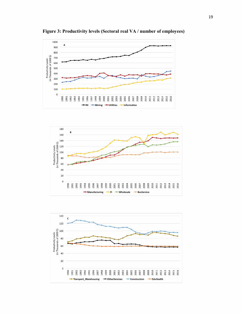
Figure 3 shows how sectoral productivity levels evolved over time. Several points stand

out, especially in light of recent debate about the extent to which rising business monopoly

power has led to more income inequality.

Figure 3

One observation is that aside from business services in panel B, the stagnant sectors are

grouped in the low productivity panels C and D. Along with business services, they show

sluggish or negative productivity growth combined with rising employment. One is tempted to

assume that holding down productivity was a means for business to create low end, low wage

jobs for workers evicted from high productivity sectors. Productivity did rise in retail, a large

low-wage employer. Its employment share fell as demand growth did not offset its productivity

increases.

In the high productivity panel A, all four output/employment ratios grew. Real estate

rental and leasing as noted above is an outlier. The utility and mining sectors are traditionally

assumed to include “natural” monopolies, while information has privileged access to data that it

7 In a bit more detail, a sector’s total cost can be broken down into costs of intermediate inputs and value-

added. Double deflation treats real value-added as a residual and so focuses on the interindustry structure

of production. Current price estimates tend to estimate levels of output and value-added directly, making

intermediate costs the residuals. Double deflation is less reliable for a sector when it is difficult to

estimate the value of its output directly from market transactions. Simply adding up costs to determine

output then becomes unavoidable. Education may be the most important example. It almost certainly has

low productivity growth, but the estimate of -0.56% per year for education and health in Table 1 is

imprecise.

8 In a hot topic at the moment double deflation can also be used to calculate movements in “effective

protection” of real wages and profits induced by changes in tariffs on a sector’s output and intermediate

inputs, e.g. pressures on the automobile sector due to higher tariffs for steel, possibly offset by tariffs on

imported car parts and cars.

9

can exploit. In panel B, finance and insurance also has monopoly elements. The diverse

manufacturing sector has historically depended on continuing productivity growth; wholesale

trade has benefitted from advances in inventory control.

Debate rages about whether the observed excess of productivity over wage growth is due

to business “monopoly” power pushing prices up against wages or suppression of wages

resulting from labor’s failing bargaining power. Decreasing profit shares suggest that monopoly

is not rampant in stagnating sectors. Among the dynamic sectors real estate rental and leasing

accounts for a stable 30% of total profits. Property owners no doubt wield market power, but it

does not appear to have strengthened over time. Manufacturing and information together account

for a quarter of profits and wholesale and retail trade for another one-eighth. As noted above,

these large profits flow mostly to high income households, leading to rising income inequality.

The bottom line, perhaps, is that productivity increases may have gone along with

monopoly power in dynamic sectors (and some sub-sectors). Productivity growth did not

accelerate, suggesting that increased monopoly did not play a role. In panels C and D,

employment increases may provide a better explanation than monopoly for slow or negative

productivity growth and the wage lag. In a relevant illustration, Montier and Pilkington (2017)

point out that the US productivity soared during WW II and collapsed thereafter, precisely in line

with its definition as a ratio of independently driven numbers including the size of the available

civilian labor force in the denominator.

Across the 16 sectors, overall productivity growth can be decomposed into a weighted

average of own-rates of increase and “reallocation” effects due to labor movements.9 For

instance, an increase in employment in a low productivity sector reduces economy-wide

productivity growth.

Figure 4 presents the sectoral contributions. Toward the right, job growth in education

and health, and accommodation and food cuts visibly into overall productivity. Toward the left,

real estate and manufacturing have real output shares in the range of 12-15% and make strong

productivity contributions. Shares of finance and insurance, retail, wholesale, and information

cluster above five percent. Table 1 shows that all these sectors had visible own-productivity

9 The weights are sectoral shares in output for productivity growth and differences between output and

employment shares for growth of employment. If its output share exceeds its employment share, a sector

has relatively high productivity so that if its employment rises there is a positive contribution to overall

productivity growth.

10

growth, explaining the pattern in Figure 4. Business services is a large sector at around 15% but

its slow own-productivity growth means that it did not contribute very much economy-wide.

Figure 4 here

Employment growth

Productivity shifts provide a means to explore movements in overall employment. At the

aggregate level, is true that

Employment ÷ Population = (Output ÷ Population) ÷ (Output ÷ Employment)

or

Employment ratio = Output per capita ÷ Productivity .

This formula provides the basis for a decomposition of growth in the employment ratio over time

as a weighted average of growth rates of sectoral outputs per capita minus growth rates of

productivity. The weights are sectoral employment shares. Using working age population for

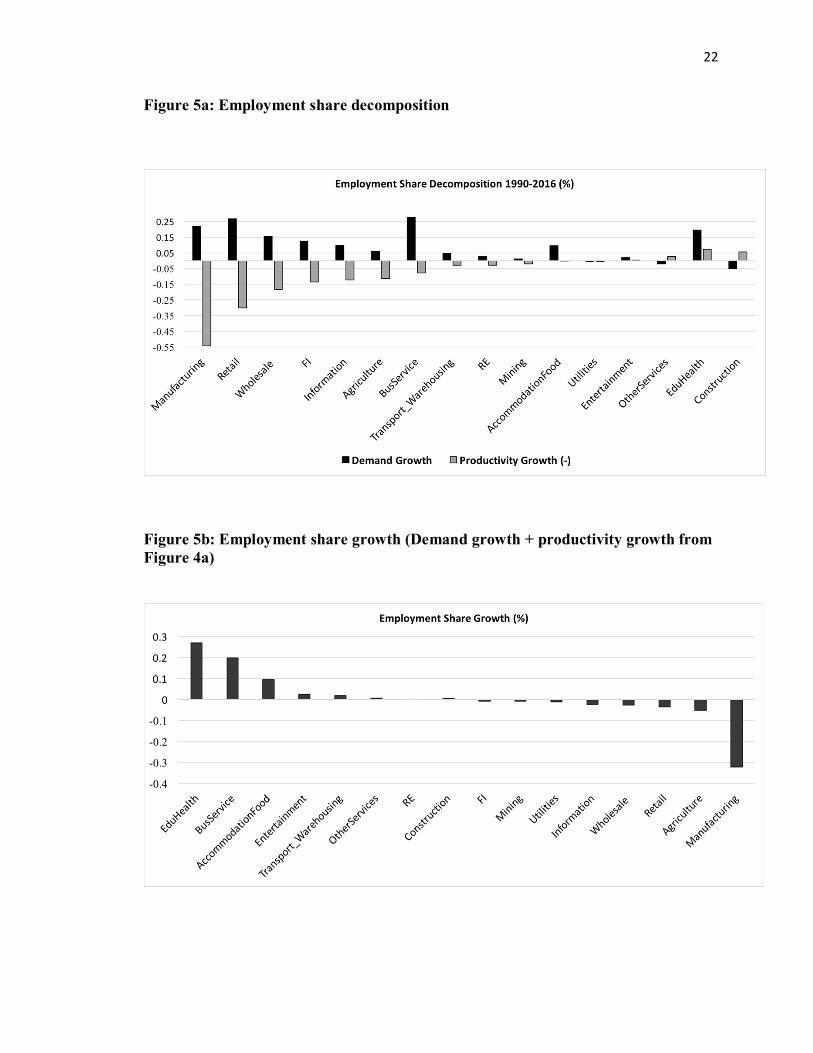
convenience, Figure 5a presents the results.

Figure 5a here

In the relatively large manufacturing sector, productivity growth outstripped demand

growth, so jobs were destroyed. There was a rough balance in the other sectors toward the left.

Demand growth along with stagnant productivity led to job creation in business services and

accommodation and food. Both demand expansion and falling productivity pushed up

employment in education and health.

Figure 5b shows the combined effects on the employment ratio of output and productivity

changes. The bulk of job creation took place in the seven sectors pointed out above (and

grouped toward the bottom of Table 1). In increasing order, job annihilation took place in

information, wholesale, retail, agriculture, and manufacturing. Robotization, the latest

manifestation of the trend toward automation that has run for more than two centuries, no doubt

contributed to slower job growth, mostly by blocking young entrants into the industrial labor

force.

11

Notably, there are 36 weekly employment hours for business services; education and

health, 33; and accommodation and food, 26. Manufacturing has 41 weekly hours. In effect jobs

shifted toward sectors with both low wages and short hours.10

Figure 5b here

Terms of trade

Given the way the numbers are calculated, the main signal that a sector is enjoying

productivity growth is that the current price value of its “real” output is falling relative to the rest

of the economy. In other words, its “terms of trade” are deteriorating. The terms of trade will

shift in favor of a sector with lagging productivity in line with the “Baumol effect” (Baumol and

Bowen, 1966).11

Automobiles have become relatively less expensive over time while the cost of

health care has gone up

The last column of Table 1 shows sectoral growth rates of double-deflated, chain-indexed

value-added. One immediate observation is that manufacturing grew less rapidly than other

sectors, e.g. its own computer and electronics sub-sector, information, wholesale and retail trade,

and finance and insurance. Slower output growth in manufacturing is to be expected in light of

historical experience worldwide.12

Sectoral real growth rates can be compared to the rates shown in the second-last column,

which were calculated by deflating value-added in current prices by an overall price index called

the GDP deflator. Differences between the two columns reflect productivity trends. The lagging

seven sectors at the bottom of the table all had (deflated) current price growth rates that exceeded

10

One might add “and multiple jobs…” About five percent of US workers hold more than one job, with

the number apparently rising. 11

The “effect” is often interpreted as stating that real wages tend to rise in industries with slow

productivity growth, pushing up costs. For the data summarized in Table 1, this version of Baumol’s idea

is not true. It can be rejected on accounting grounds alone. The real (product) wage equals labor

productivity times the wage share. Such shares are relatively stable so that growth of the wage will be

roughly proportional to growth of productivity. The fact that in Table 1 wages lag productivity in low end

sectors means that profits have benefitted most from Baumol effects.

12

In European examples according to World Bank data, the manufacturing share of real GDP in Germany

fell from 25% in 1991 to 21% in 2017, and in Sweden from 21% in 1980 to 14% in 2016. The decrease in

the USA was from 16% in 1997 to 12% in 2016.

12

their real rates. The implication is that prices shifted in their favor. With a few exceptions, the

opposite is true of the remaining sectors. The real vs. current price growth rate differential for

computers is particularly striking.13

Stagnant and dynamic sectors

The evidence shows that the seven sectors toward the bottom of Table 1 fall behind in

profits , labor income, and output while creating employment. The ones toward the top of the

table have high and rising productivity, albeit with real wage suppression. Models of

interactions between “dynamic” and “stagnant” sectors proposed by Rada (2007) and Storm

(2017) help explain the discrepancy.

Both papers assume that workers who do not find dynamic sector jobs are driven into the

stagnant part of the economy. To paraphrase Storm for rich economies, especially the USA, this

“full employment” assumption reflects the fact that in the absence of unemployment insurance

and social security worth the name, workers must find jobs, if not in the better paid core, then in

a low end sector in some peripheral activity. In contrast to standard models, endogenous

adjustment of productivity in the stagnant sector allows “full” employment (supplemented by

fiscal transfers) to be maintained.

This idea traces back to debates in development economics a half-century ago. Lewis

(1954) proposed that poor countries have “surplus labor” (or a “reserve army” in Marx’s

terminology) which can be brought from subsistence activity into employment in an expanding

modern sector. Sen (1966) pointed out that subsistence output would change very little as labor

moved in and out of the sector. In a reversed version of Lewis’s narrative, Sen’s idea suggests

that productivity should fall in proportion to the quantity of labor moving into the stagnant zone,

or that the elasticity of productivity with respect to employment equals minus one, in a strong

case of decreasing returns. Slow productivity growth in the face of rising employment for the

13

On the assumption that prices are largely driven by labor costs, the older literature on international

trade traced shifts in the “double factorial terms of trade” to differences between wage growth minus

productivity growth across countries. In the current context if wage growth rates are equal, a negative

difference of this indicator between dynamic and stagnant sectors arises if productivity growth is higher

in the former than the latter (as in Table 1). That is, prices shift against the dynamic sectors due to

productivity growth differentials.

13

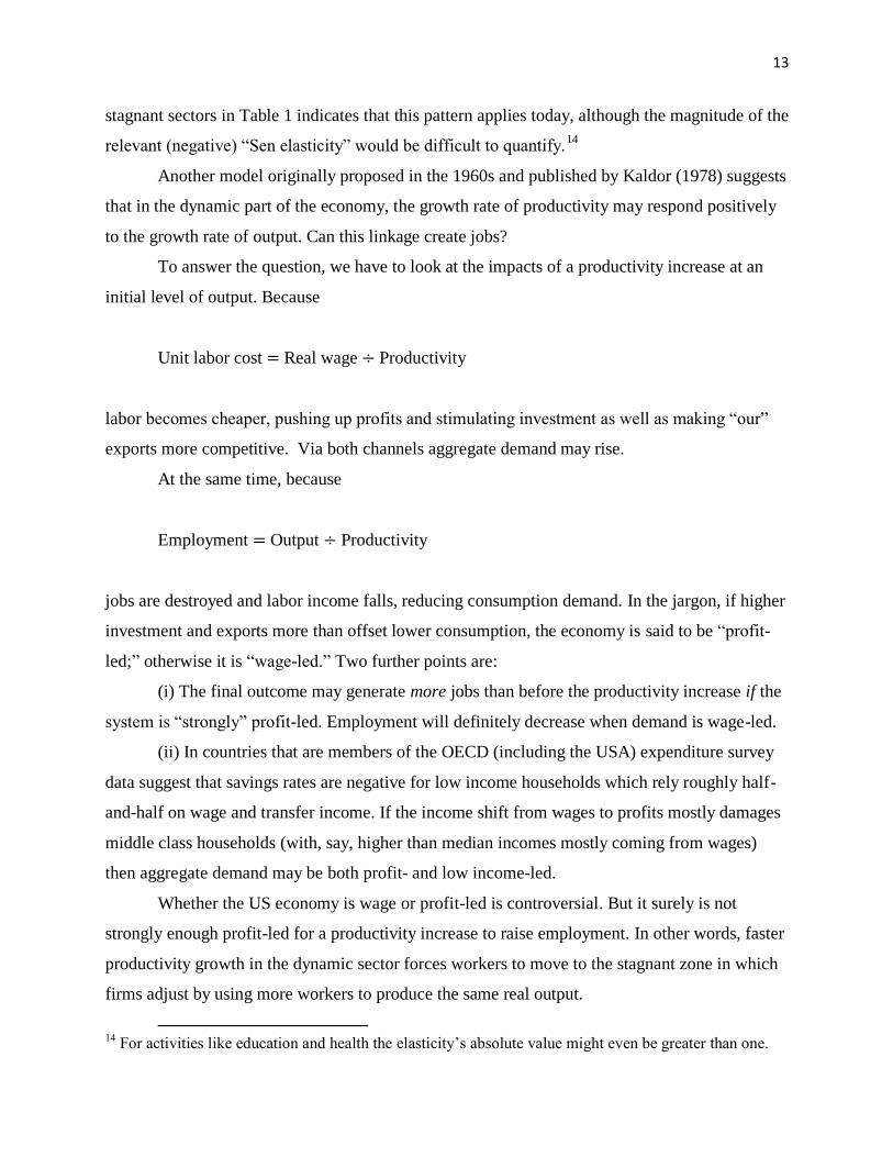
stagnant sectors in Table 1 indicates that this pattern applies today, although the magnitude of the

relevant (negative) “Sen elasticity” would be difficult to quantify.14

Another model originally proposed in the 1960s and published by Kaldor (1978) suggests

that in the dynamic part of the economy, the growth rate of productivity may respond positively

to the growth rate of output. Can this linkage create jobs?

To answer the question, we have to look at the impacts of a productivity increase at an

initial level of output. Because

Unit labor cost = Real wage ÷ Productivity

labor becomes cheaper, pushing up profits and stimulating investment as well as making “our”

exports more competitive. Via both channels aggregate demand may rise.

At the same time, because

Employment = Output ÷ Productivity

jobs are destroyed and labor income falls, reducing consumption demand. In the jargon, if higher

investment and exports more than offset lower consumption, the economy is said to be “profit-

led;” otherwise it is “wage-led.” Two further points are:

(i) The final outcome may generate more jobs than before the productivity increase if the

system is “strongly” profit-led. Employment will definitely decrease when demand is wage-led.

(ii) In countries that are members of the OECD (including the USA) expenditure survey

data suggest that savings rates are negative for low income households which rely roughly half-

and-half on wage and transfer income. If the income shift from wages to profits mostly damages

middle class households (with, say, higher than median incomes mostly coming from wages)

then aggregate demand may be both profit- and low income-led.

Whether the US economy is wage or profit-led is controversial. But it surely is not

strongly enough profit-led for a productivity increase to raise employment. In other words, faster

productivity growth in the dynamic sector forces workers to move to the stagnant zone in which

firms adjust by using more workers to produce the same real output.

14

For activities like education and health the elasticity’s absolute value might even be greater than one.

14

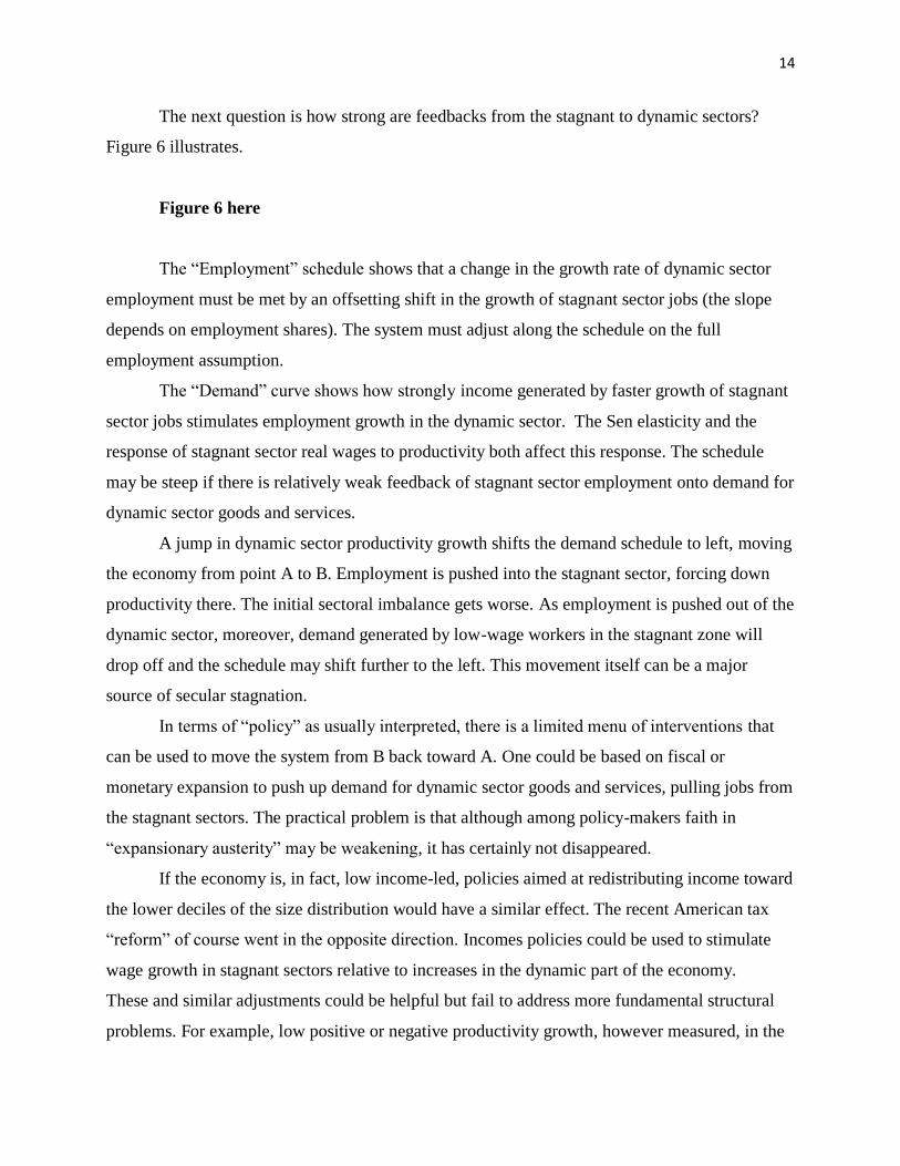
The next question is how strong are feedbacks from the stagnant to dynamic sectors?

Figure 6 illustrates.

Figure 6 here

The “Employment” schedule shows that a change in the growth rate of dynamic sector

employment must be met by an offsetting shift in the growth of stagnant sector jobs (the slope

depends on employment shares). The system must adjust along the schedule on the full

employment assumption.

The “Demand” curve shows how strongly income generated by faster growth of stagnant

sector jobs stimulates employment growth in the dynamic sector. The Sen elasticity and the

response of stagnant sector real wages to productivity both affect this response. The schedule

may be steep if there is relatively weak feedback of stagnant sector employment onto demand for

dynamic sector goods and services.

A jump in dynamic sector productivity growth shifts the demand schedule to left, moving

the economy from point A to B. Employment is pushed into the stagnant sector, forcing down

productivity there. The initial sectoral imbalance gets worse. As employment is pushed out of the

dynamic sector, moreover, demand generated by low-wage workers in the stagnant zone will

drop off and the schedule may shift further to the left. This movement itself can be a major

source of secular stagnation.

In terms of “policy” as usually interpreted, there is a limited menu of interventions that

can be used to move the system from B back toward A. One could be based on fiscal or

monetary expansion to push up demand for dynamic sector goods and services, pulling jobs from

the stagnant sectors. The practical problem is that although among policy-makers faith in

“expansionary austerity” may be weakening, it has certainly not disappeared.

If the economy is, in fact, low income-led, policies aimed at redistributing income toward

the lower deciles of the size distribution would have a similar effect. The recent American tax

“reform” of course went in the opposite direction. Incomes policies could be used to stimulate

wage growth in stagnant sectors relative to increases in the dynamic part of the economy.

These and similar adjustments could be helpful but fail to address more fundamental structural

problems. For example, low positive or negative productivity growth, however measured, in the

15

dysfunctional American health care system is devastating. Employment in manufacturing,

historically the main locus of productivity growth, will probably remain weak. Income

elasticities of demand for the whole range of manufactured final goods (or “stuff”) and even

intermediates are not likely to rebound even as productivity growth continues. Globalization and

international trade have taken a toll in terms of jobs, not only in manufacturing. Offshoring the

production of intermediate inputs such as computer code cuts costs and raises the productivity of

remaining workers in the USA. Creative destruction of onshore jobs still is destruction. Its

impact may be stronger if investment in new technologies shifts from the USA to abroad.

Falling or stable wages in stagnant sectors is exacerbated by non-poaching and non-

competition clauses in contracts (which restrict job opportunities outside a company for a worker

who leaves it). Divide-and-rule employment tactics in a “fissuring” labor market as described by

Weil (2014) are another aspect of this process.

All these factors tend to push the demand schedule in Figure 6 to the left. There are

countervailing powers but stagnation may well worsen unless they soon grow stronger.

16

References

Baumol, William, and William Bowen (1966) Performing Arts: The Economic Dilemma, New

York: Twentieth Century Fund.

Congressional Budget Office (2018) “The Distribution of Household Income, 2014”

https://www.cbo.gov/publication/53597

Hicks, John R. (1932) The Theory of Wages, London: Macmillan

Kaldor, Nicholas (1978) “Causes of the Slow Rate of Growth of the United Kingdom” in Further

Essays on Economic Theory, London: Duckworth

Lewis, W. Arthur (1954) “Economic Development with Unlimited Supplies of Labor,”

Manchester School, 22: 139-19.

Montier, James, and Philip Pilkington (2017) “The Deep Causes of Secular Stagnation and the

Rise of Populism,” GMO White Paper (Grantham, Mayo, Van Otterloo)

Moyer, Brian C., Mark A. Planting, Mahnaz Fahim-Nader, and Sherlene K. S. Lum (2004)

“Preview of the Comprehensive Revision of the Annual Industry Accounts,

https://www.bea.gov/scb/pdf/2004/03March/0304IndustryAcctsV3.pdf

Rada, Codrina (2007) “A Growth Model for a Two-Sector Economy with Endogenous

Employment,” Cambridge Journal of Economics, 31: 711-740

Semieniuk, Gregor (2018), “Energy in Economic Growth: Is Faster Growth Greener?” SOAS

Department of Economics Working Paper Series, No. 208, SOAS University of London.

Sen, Amartya (1966) “Peasants and Dualism with and without Surplus Labor,” Journal of

Political Economy, 74: 425-450.

Storm, Servaas (2017) “The New Normal: Demand, Secular Stagnation, and the Vanishing

Middle-Class,” https://www.ineteconomics.org/uploads/papers/WP_55-Storm-The-New-

Normal.pdf

Taylor, Lance, and Özlem Ömer (2018) “Where do Profits and Jobs Come From? Employment

and Distribution in the US Economy,”

https://www.ineteconomics.org/uploads/papers/WP_72-Taylor-and-Omer-April-8.pdf

Taylor, Lance (forthcoming) The Rise of the Rentier: Soaring Economic Inequality from Reagan

to Trump and What is to be Done, New School for Social Research

Temin, Peter (2017) The Vanishing Middle Class: Prejudice and Power in a Dual Economy,

Cambridge MA: MIT Press

Weil, David (2014) The Fissured Workplace, Cambridge MA: Harvard University Press.

17

Figure 1: Productivity growth vs product wage growth 1990-2016 (trend lines omit

real estate and computers)

Figure 2: Productivity levels vs. growth rates 1990-2016

18

Table 1: Summary data for the sectors

Table 2a: Total household incomes by source and stagnant and dynamic sectors (trillions of

2014 dollars)

Wages Non-wage Transfers Financial Totals

Stag. Dyn. Stag. Dyn. Stag. Dyn. Stag. Dyn. Stag. Dyn.

Low 1.2 1.0 0.1 0.2 1.0 0.9 0.1 0.1 2.4 2.2

Middle 3.5 2.8 0.4 0.5 0.4 0.2 0.5 0.4 4.8 3.9

High 0.8 1.2 0.8 2.8

Table 2b: Mean incomes per household by source and stagnant and dynamic sectors

(thousands of 2014 dollars)

Wages Non-wage Transfers Financial Totals

Stag. Dyn. Stag. Dyn. Stag. Dyn. Stag. Dyn. Stag. Dyn.

Low 27 34 2 7 22 31 2 3 53 75

Middle 119 150 14 27 14 11 17 21 164 209

High 667 1000 667 2334

19

Figure 3: Productivity levels (Sectoral real VA / number of employees)

20

21

Figure 4: Decomposition of labor productivity growth (using double deflated output

levels)

22

Figure 5a: Employment share decomposition

Figure 5b: Employment share growth (Demand growth + productivity growth from

Figure 4a)

23

Figure 6: Effects of an upward shift of productivity growth when the dynamic sector

is not strongly profit-led