NASA-TM-II2169//_,"

Y q

THE SCHWINGER VARIATIONAL METHOD

Winifred M. Huo

NASA Ames Research Center, Moffett Field, CA 94035, U.S.A.

1. INTRODUCTION

Variational methods have proven to be invaluable tools in theoretical physics and

chemistry, both for bound state problems and for the study of collision phenomena. For

collisional problems variational methods can be grouped into two types, those based on

the SchrSdinger equation and those based on the Lippmann-Schwinger equation. The

I-Iulth_n-Kohn 1-3 method belongs to the first type, and their modern development for

electron-molecule scattering, incorporating complex boundary conditions, is reported in

chapter 1 of this book by Rescigno et al. 4 An offshoot of the Hulth_n-Kohn variational

method is the variational R-matrix method, s' _ In chapter 8 of this book Schneider r

presents a general discussion of the R-matrix method, including the variational R-

matrix.

The Schwinger variational (SV) method, which Schwinger introduced in his lectures

at Harvard University and subsequently published in 1947, s belongs to the second

category. The application of the SV method to e-molecule collisions and molecular

photoionization has been reviewed previously. 9-12 The present chapter discusses the

implementation of the SV method as applied to e-molecule collisions. Since this is not

a review of cross section data, cross sections are presented only to serve as iUustrative

examples.

In the SV method, the correct boundary condition is automatically incorporated

through the use of the Green's function. Thus SV calculations can employ basis func-

tions with arbitrary boundary condition. This feature enables the use of an L 2 basis for

scattering calculations, and provided the initial motivation for applying the SV method

to atomic and molecular physics) °' lz The initial success led to the development of the

iterative Schwinger method 14 which uses single-center expansion techniques and also an

iterative procedure to improve the initial basis set. The iterative Schwinger method has

been used extensively to study molecular photoionization, is For e-molecule collisions,

it is used at the static-exchange level to study elastic scattering 16 and coupled with the

distorted wave approximation to study electronically inelastic scattering) 7

The Schwinger multichannel (SMC) method, originally formulated by Takatsuka

and McKoy, is t9 is the first modern computational method for e-molecule collisions ex-

phcitly designed to treat the multicenter nature of a polyatomic target. When Gaussian

Computational Methods for Electron-Molecule Collisions

Edited by W.M. Huo and F.A. Gianturco, Plenum Press. New York, 1995 327

https://ntrs.nasa.gov/search.jsp?R=19970009402 2018-06-22T23:15:05+00:00Z

functions are used for the L 2 basis and plane waves for the incoming electron, all two-

electron repulsion integrals are calculated analytically. It is also a multichannel method

and readily treats electronic inelastic scattering as well as polarization effects in elastic

scattering. In addition, integrals involving the Green's function, generally considered

the bottleneck in the SV method, can now be computed efficiently and accurately us-

ing the insertion method. 2° Alternatively, highly parallel computing can be effectively

employed in the numerical integration over the final three-dimensions for this type of

integrals) 2 The SMC method has been found to be robust, and has been employed to

study molecules of various sizes and with different bonding types. For example, it has

been used to study the electronic excitation of [1,1,1] propeUane by electron impact, _1the largest polyatomic molecule studied so far by ab initio methods. It has also been

used to study electron scattering from the ground state of BeCO, a molecule with a

weak van der Waals bond, to simulate scattering from an adsorbate in a physisorbedsystem. 22 Since the SMC method is the most commonly used SV treatment for e-

molecule scattering, the main topic of this chapter will deal with its implementation.

Both the SMC and iterative Schwinger methods calculate fixed-nuclei, body-frameT-matrices. Domcke 23 has demonstrated that nuclear dynamics in e-molecule collisions

can be treated efficiently using projection operator formalism and Green's function

approach. Results of the fixed-nuclei SMC calculation can be coupled directly with

Domcke's treatment of nuclear dynamics. As an example, we present a calculation of

vibrational excitations of N2 by electron impact which combines these two treatments.

2. THE LIPPMANN-SCHWINGER EQUATION AND THE SCHWINGERVARIATIONAL PRINCIPLE

In the integral equation approach, we look for solutions of the Lippmann-Schwinger(LS) equation instead of the SchrSdinger equation. Let the Hamiltonian of the electron+ molecule system be written as

H=_ -_V,- Ir,;it_l + _--,=1 (1)i

= l>k

Here i,j and k,l sum over electrons and nuclei, respectively; Z_ and rnk denote the

charge and mass of the kth nucleus. Also, atomic units will be used unless specified

otherwise. Note that H is symmetric and its eigenfunction antisymmetric with respectto electron exchange. Rewriting H as

with

and

H = Ho+ V, (2)

1 2

Ho= HM -- _VN+,, (3)

Jv 1 Jvp Zk

__ +.V = {=t_IrN+, - r,I = Ir_v+t _ R_ I (4)

The use of N + 1 to label the continuum electron is completely arbitrary. Also, HM isthe molecular Hamiltonian with eigenfunctions q,,,,

H,,+_ = E,_+_. (5)

328

The LS equation is given by,

eft+) = S + G(+)Vgfl +). (6)

with

hm(E - Ho + ig)G(+)(E ') = 5(E - E'). (7)

and S is the solution of the corresponding homogeneous equation) / Here we use the

boundary condition of an incoming plane wave and outgoing spherical waves, which

has been incorporated into the Green's function G (+). Due to this feature, it is not

necessary to use trial functions which satisfy the correct boundary conditions in solving

the LS equation. The Green's function G (+) is expressed in terms of the molecular

eigenfunctions and the interaction-free Green's function.

1 ezp(ik,,,IvN+l -- VN+, '1)(ff-,[. (8)G(+)(E) = -_ _-" 1_") Iv_r+l- vN+I'I

rrt=l

where -lk2 + £,,, = E, (9)2 "

The summation m is over the entire molecular spectrum, including continuum states.

When £,,, > E, k,_ becomes imaginary, corresponding to a bound electron. Indeed,

including the continuum spectrum of the target allows the outgoing electron to be

different from the incoming electron, a necessary feature in order to account for electron

exchange. 2/

Based on the LS equation for ql(+) and the corresponding equation for _(-) with

outgoing plane wave and incoming spherical waves boundary conditions,

q_(-) = S + G(-)V@ (-).

the Transition matrix, or T-matrix, of a scattering process can be written as

T,,,,, = (s,.IVl_.(+)> = (_(_-)lVlS,) = (_(_-)lV - VG(+)VI(,(.+)>. (10)

It is readily seen that a combination of the above expressions

T,,,, = (S,,,IVI_I'(,+)) + (_I'L-)IVIS,,) - (_2_-)1V - VG(+)VI_(.+)) • (11)

results in a T-matrix that is stationary with respect to first-order variations in tI'(+)

and _I'(-), respectively.

6T,,,.= <SmlVlgfl+) + 5g/(_+)>+ <_(_-)IVIS.>- <_-)lv- va(+)vl_(.+)+ 6_(.+)>- Tin.

=0,

t/ We choose to use a homogeneous solution which is the product of the target wave function and

the free-particle wave function of the continuum electron, without antisymmetrization between the

two. As pointed out in Ref. 24, it is not necessary to antisyrametrize both the initial and final wavefunctions explicitly. If ¢fl+) is antisymmetric, then the T-matrix element will automatically pick up

the antisymmetric part of S. This convention is used here so that the same S will also apply to the

SMC equation discussed in See. 3.2/ A different approach to account for exchange is to incorporate the Hamiltonian with permuted

indices into the interaction potential, U = V + _, P_,N+I(H - E). See Bransden et al. 2s

329

and

_fTm,= (S,,IVIfi (+)) + (02(-) + ,ffi(-)lV]S,) - (02(-) + _fi(-)]V - VG(+)VI02 (+)) - T,,,,_

---_0.

Equation (111 is referred to as the linear form of the Schwinger variational principle.

In most e-molecule calculations, it is common practice to expand 02(+) and fig(-) in

terms of a set of antisymmetrized N + 1-electron trial functions f,

(12)fig(.+)= E b,(_.)/.,

and

fi(_-)= Z c.(km)L. (13)$

Eq. (1 1) gives

T,,, = __, b,(S.,IVIf,) + __, c,(f, lVIS.) - __, __,b,c,(f.IV - VG(+)VIf,). (14 /r • .r .$

The requirement that Tmn be stationary with respect to first order variations in the

expansion coefficients br and c,,

OTmn/Ob,. = O,

cOTm,_/ Oc, = O,

gives the following relationships,

with

b. = __.D.(LIVIS,,),$

c, = _(SmlVlf,>D.,

(15)

(16)

(17)

(18)

(D-l),, = (f,)V - VG(+)V]f,).

The resulting variational stable expression for T,m is 28

Tm,_ = ___(S,_IVIf.>D.<f.IV[S,, >.r$

Equation (18) has the advantage that it is independent of the normalization of 02_+)

and fi(-).

The advantages of the Schwinger variational method have been discussed prev-

iously.9.10 Because the correct boundary condition is already incorporated into the

Green's function and because the variational stable expression of the T-matrix in

Eq. (18) is independent of normalization, it allows flexibility in the choice of a ba-

sis. Furthermore, the wave function in Eqs. (11) and (18) always appears together with

the potential, i.e., Vlfi(+) ) or (fi(-)]V. Thus a trial basis for fig(+) needs only to cover

the region of space where V does not vanish. This feature allows us to use an L 2 basis

to represent fig(+) when V is a short-range potential.

Another advantage of the SV method is that the Schwinger variational principle is

one rank higher than the Kohn variational principle. :_' 2s If the same trial wave function

is used, the Schwingcr method should give a better converged result. It should be noted

330

that, in comparing the two methods, it is important to use the same trial basis because

the Kohn method, which requires basis functions with the correct boundary condition,

generally uses a trial basis different from the Schwinger method.

A major drawback of the SV method lies in the difficulty in calculating the Green's

function matrix elements. 9 The matrix element (9(.:)lvc(+)vIg(_ +)) in Eq. (11) or

(f, IYG(+)Vf.f, ) in Eq. (17) are nine-dimensional integrals if V includes a two-electron

potential. This obstacle has recently been removed when it is demonstrated 2° that the

insertion technique can be used with efficiency and good accuracy for the evaluation of

these matrix elements. This will be discussed in Sec. 3.5. Alternatively, highly parallel

computing can be employed for the 3-dimension numerical integration over the wave

vector in these matrix elements.

2.1. A Simple Example of Potential Scattering

To illustrate the use of Eq. (18) and to demonstrate the convergence property of

the SV method, consider the elastic scattering of an s-wave by a weak potential U. The

initial state is described by the Riccati-Bessel function,

S = j0(kr).

Since the potential is weak, j0(kr) can also be used as a reasonable representation for

the trial functions of 9 + and 9(-). Here the trial functions are of the form

9 (+) = bojo(kr),

9 (-) = cojo(kr).

Because the initial boundary condition is described by S in the LS equation, the coef-

ficients b0 and Co need not be set to 1. Instead, they are used as variational parameters

and optimized. Note that the use of j0(kr) as a trial basis is an example of a basis

which does not satisfy the correct boundary condition. Otherwise a combination of

Riccati-Bessel and Neumann functions should be employed. Because 9 (+) and 9(-) are

expanded in a one term expansion, the inverse of the D-matrix, in Eq. (17), is just the

inverse of the matrix element itself. From Eq. (18), the SV expression of the elastic

T-matrix is given by

(jo( kr ) [g ljo( kr )) (jo( kr ) ]U ljo( kr ))

Too = (jo(kr)l U _ UG(+)Uljo(kr))

Since U is a weak potential, we can write

1 1 (jo(kr)lUG(+)gljo(kr))+ ...).

(jo(kr)lU - Ua(+)Uljo(kr)) -- (jo(kr)lU]jo(kr)) (1 + (jo(kr){Uljo(kr))

Substituting the above into the expression for Too, we find

Too = (jo(kr)lUIjo(kr)) + (jo(kr)lUG(+)Uljo(kr)) +""

The first and second terms of Too correspond to the first and second Born terms, re-

spectively.

In Eq. (10) three non-variational expressions for Too are given. They give identical

results if the exact q2(+) and 9(-) are used. Otherwise they give different values for the

T-matrix. The first relation,

Too = (SIUIg(+)),

331

gives the Born approximation for Too.s�

Too = (jo(kr)lUljo(kr)).

This result is inferior to the SV expression. Using the third relation in Eq. (10),

Too= (_(-)IU - UG(+)UI_(+)>,

Too deviates even further from the variationaUy stable result,

Too = (jo(kr)]Utjo(kr)) -(jo(kr)]UG(+)Ufjo(kr)).

Now the second Born term is subtracted from, instead of added to, the first Born term.

The above exercise clearly illustrates the power of the variational method.

3. THE SCHWINGER MULTICHANNEL METHOD (SMC)

Currently, the most frequently used form of the Schwinger variational principle for

e-molecule collisions originates from the work of Takatsuka and McKoy) s' i0 As seen be-

low, while this formulation is based on the Schwinger variational principle, its equation

of motion is obtained by combining the LS and SchrSdinger equations. These equations

are coupled via the introduction of a projection operator P which projects into the open-

channel target space. In the following, we shall first consider some of the properties of

Takatsuka's projection operator, then derive the SMC equation. Implementation of themethod will then be defineated. Efficient evaluation of the Green's function matrix el-

ements, generally considered a bottleneck in the Schwinger method, will be discussed

and extension to include correlated target functions will also be presented.

3.1. The N-Electron Projection Operator P

The projection operator P introduced by Takatsuka and McKoy projects into the

open channel target space. Hence it is an N-electron projection operator and different

from the Feshbach projection operator, 29 which is a N + 1-electron operator.

M

P = _ [¢,,(1,2,...,N))(¢,,(1,2,...,N)[, (19)rrt=l

with m summing over all energetically accessible target states. P satisfies the idempo-tent property,

p2 = p,

and commutes with Ho

PHo = HoP.

To illustrate the difference between P and PN+I, the Feshbach projection operator,

consider the simplest case when the target wave function ff_ is expressible in terms ofa closed shell, single determinental wave function,

• ,(1,2,..., N)= .A {qblct(1)¢at3(2)...¢N/_a(N 1)¢N/2/3(N)}.

a/ Here q/(+) is not optimized and bo : 1 is used.

332

Here a and/3 denote spin functions and .A the antisymmetrizer. If the wave function

of the continuum electron, 9i(N + 1), is orthogonal to all the target orbitals, then the

Sz= 1/2 component of q/i becomes

_,(1, 2,..., N, N + 1) = A {¢1a(1)¢1/3(2)...¢N/2/3(N)g,a(N + 1)}.

We have

P_,(1,2, N,N+ 1) - 1 (Ih(1,2,... N)g,a(N+l), (20)

and 1

(kVj]HPI_,) - N + 1 (_j[H[_,). (21)

On the other hand, the Feshbach projection operator is defined in terms of the N + 1-

electron open channel functions,

PN+I = _ [_m(1,2,...,N,N + 1))(q_m(1,2,...,N,N + 1)[.m

where kOm satisfies the correct asymptotic boundary condition. The function q2i is an

open channel function in the terminology of the Feshbach projector formahsm if glsatisfies the correct boundary condition. In that case,

PN+lq2i = q2i. (22)

A comparison of Eqs. (20) and (22) shows how the two projection operators differ. Alsonote that Takatsuka's projection operator treats kvi as an open channel function as

long as it is associated with an energetically accessible target function, regardless of the

behavior of gi at the boundary. The Feshbach projection operator, on the other hand,

includes _i in the open channel space only if gi has the correct boundary behavior.It should be noted that Eq. (20) may not be apphcable when the orthogonahty

constraint between the continuum electron function and the target function is relaxed,

and/or when the target is described by more sophisticated wave functions. Consider

the simple case of X Eg_1 + bZ+E, excitation of H2 by electron impact. Let the wave

function for the 1 +X Eg state be represented by

_x = A{l_ga(1)lera/3(2)},

b E_ state byand the three spin components of the 3 +

¢b.S.=l = A{laga(1)la.a(2)},

A{lao(1)1o-_,(2)_ 2 [a(1)/3(2) + fl(1)a(2)] },_b,s,=o

• b,s,:-, = A{1ag/3(1)1w_/3(2)}.

It is well established that in calculating this transition, terms of the form

¢o = A{la0_(1)laoa(2)la_/3(3)}, (23)

and(24)

333

shouldbeincludedin theexpansionofthewavefunction.Theseareusuallycalled'pen-etration'or 'recorrelation terms' because they relax the enforced orthogonality between

the continuum and target functions. Let the projection operator P be generated fromthe four target functions above. We then have

1 1P_, : _ ,.s,=l(1,2)la_fl(3) v_¢b.s.:o(1,2)lc%a(3). (25)

This simple example illustrates how the operation of P depends on the type of functionsused,

3.2. The SMC Equation

The projected LS equation is

= f,(+) 1:,r,(+)Pq'_+) &+_'v -=, ,

The projectec Green's function, G(p+), is defined in the open channel space by,

Gtp+) _ 1 M2_ _ [era) ezP(i<'[":'+a - ":'+1 t)(¢ml'

(26)

rn=l

Multiplying Eq. (26) from the left by V and rearranging, we find

(VP - VG(p+)V)qt_ +) = VSn (27)

Equation (27) describes only the open channel functions, whereas a complete de-

scription of q'_+) also requires the closed channel component. To do this, we use thefollowing identity

aP + (1 - aP) = 1. (28)

Note that in association with the operation of P, a parameter a, called the projection

parameter, is introduced. It is seen from Eqs. (20) and (25) that the operation of Pnot only removes the antisymmetrization between the target function and continuum

orbital, but also generates a constant which multiplies the resulting function. Thus the

introduction of a is a logical step. The determination of a will be discussed after theSMC equation is derived.

The closed channel contribution is described by the projected SchrSdinger equation,

(1 - aP)[Iq2(+) = O,

with

and

(29)

flo=E-Ho.

P[f = P[-Io - PV

1 PHo) By= _( oF + -

Note that

= _(HP + P[I) + _(VP - PV).

334

Equation (29) can be rewritten as

I//- (,qP + P/Z)+ 2(Pv - vp)l¢+): o. (30)

The SMC equation is obtained by dividing Eq. (30) by a and adding it to Eq. (27),

A(+)¢(, +) = VS,,, (31)

with A (+) the SMC operator,

(32)

The SMC equation 4/ uses the LS equation to describe the open channel component

of _(+) and the SchrSdinger equation for the closed channel component. Because it

includes both the open and closed channel components, it provides a complete solution

to the scattering problem. 3°

Using the SMC equation instead of the LS equation, the Schwinger variational

expression for the T-matrix is

T,,,, = (g,.,,IVl_k+/)+ (q'_-)lVlS,,) - (q'_-)lA(+)l_+)). (33)

If the scattering wave function is expressed in terms of N + 1-electron trial functions

f, as in Eqs. (12) and (13), the variational stable expression for Tm_ is the same as

Eq. (18),

Tin. = _,<s,,IVIL)D,o(LIvIS,). (34),rs

but with

(D-'),, = (LIA(+)IL). (35)

3.3. The Projection Parameter a

The SMC equation is incomplete until a is chosen. A number of ways of determining

a have been considered in the literature, and they are described below:

(a) Based on the hermitieity of the principal-value SMC operator. Takat-

suka and McKoy as' 19 and Lima and McKoy 3° argued that the variational stability of

Tmn requires

A (+)t = A (-). (36)

in other words, the principal-valued SMC operator A must be Hermitian. Otherwise,

Tmn will be unstable with respect to first order variation of either 6g'! +) or 6k_-). While

Eq. (36) is readily satisfied for trial functions consisting only of L 2 functions, Takatsuka

and McKoy noted that, if the trial functions included (shielded) spherical Bessel and

Neumann (or Hankel) functions, Eq. (36) is not valid because the xnatrix element of

the kinetic energy operator between Bessel and Neumann functions is non-Hermitian.

In this case, they showed that if the projection parameter is chosen to be

a=N+l, (37)

4/ Takatsuka and McKoy's original derivation ls,19 used the principal-value SMC operator, A, obtained

by replacing G(p+) with the principal-value Green's function, Gp. Similarly, the wave functions are

replaced by those with standing wave boundary conditions. [towever, most subsequent numericalcalculations used A (+).

335

the following matrix element vanishes in the open channel space,

(p_,,[1/:/_ _(p[/+ [/pllpq. ) = O.a

The operator _/7/- ½(P/:/+/:/P) is the only part of the SMC operator which involvesthe kinetic energy operator. If its matrix element is identically zero in the open channel

space, Eq. (36) is guaranteed to hold even for a basis which includes spherical Besseland Neumann functions.

(b) Based on the stability of the T-matrix with respect to first ordervariation of a. Huo and Weatherford 31 pointed out that the SMC equation auto-

matically incorporates the proper boundary condition through the Green's function.Thus it is unnecessary to include functions with the proper boundary condition in an

SMC basis. Indeed, almost all SMC calculations carried out so far use an L 2 basis. In

that case, Eq. (36) is satisfied independent of a. Even if continuum functions are in-cluded in the basis, the use of 6-function normalizable continuum functions would again

ensure the validity of Eq. (36). (A Neumann function is not 6-function normalizable).

Instead, they considered the role of a as a weight factor for the relative contribution

between the open and closed channel space. Thus a should be treated as a variation

parameter and its optimal choice should be based on the variational stability,

OTmn/Oa = O.

If q_) and ¢2(-) are expanded in terms of Eqs. (12) and (13), the above condition results

in the following expression,

__, __b,(f,l[tlf,)c, = 0. (38)r $

Equation (38) is to be solved together with Eqs. (15) and (16) so that a can be deter-

mined simultaneously with the expansion coefficients b_ and c,.

Using Eqs. (12) and (13), Eq. (38) can be rewritten as

Thus it will be automatically satisfied if q(+) and/or q_-) satisfy the SchrSdinger equa-

tion,

or

f/_-) = O.

Under these circumstances, Tmn will be stable for any finite value of a, including

a = N + 1. This result is related to how tile LS and Schr6dinger equations are com-

bined in the SMC equation. A true solution should satisfy both equations, with the

result independent of how the SMC operator is partitioned. However, in practical cal-

culations we search for a variationally stable Tin,. Equation (38), which is identical to

the configuration-interaction (CI) equation in electronic structural calculations, is much

more amenable to practical calculations than the Schr6dinger equation itself. Generallywe have found that an iterative solution of a, coupled with the calculation of Tin,, adds

approximately 10% to thc cost of an SMC calculation with fixed a.

336

(c) Based on supplementing the projected LS equation. An alternate

proof for Eq. (37) was provided by Winstead and McKoy. 32 Instead of using the SMC

equation, they looked for the variational stability of T,,, by using the projected LS

equation, Eq. (26), alone.

Tin. = (S IVI (.+))+ <¢.,-)lVlS,>- -

While the above expression is not variationally stable, they found that stability can be

achieved by adding to the projected LS equation a term Q]/.

= v ¢+) vc(/)v + Q . ,T,,, <Sin , > + <_(-)IVIS,) _ - _f/q2(+)_, (39)

with

Q=P-R.

The operator R, applied to an antisymmetrized N + 1-electron function, removes the

antisymmetrization between an N-electron function and the one-electron function for

the (N + 1)th electron. Thus we have

1(*(-)IR/;/I*(+)) - N +

It can be readily shown that Eq. (39) leads to a variational stable expression for T,,_,

with Eq. (37) for a. However, unlike Eq. (28), the operators P and Q do not span the

complete space. In view of the fact that P is an N-electron operator whereas R, and

hence Q, is an N + 1-electron operator, we have

P+Q¢I.

In contrast with the result of Lima and McKoy 3° who used Eq. (28) to prove the com-

pleteness of the solutions of the SMC equation, the present approach fails to demon-

strate that the solution of the operator equation

(VP - VG(p+)V + QH)¢<+) = S,

is complete.

3.4. Implementation of the SMC Method

The trial wave function q/(+) in the SMC method is expanded by

M

*(.+) EZ (°) "= b,j A{OI(1...N)xj(N + 1)} + _bl")®t(1 .N + 1),

i=1 j 1

(40)

where the index i sums over open channel target functions, j sums over the one-electron

basis set X used to expand the continuum electron function, and I sums over 0, the

antisymmetrized N + 1-electron configuration-state-function (CSF). The expansion co-

efficients b17 ) and bl '*) are to be determined variationally.

So far, all SMC calculations on molecules have used target functions represented by

a Cartesian Gaussian basis. Also, they make use of the fact that the correct boundary

conditions have been automatically incorporated in the SMC equation and employ an

L 2 basis of Cartesian Gaussian functions to represent the contimtum electron. Thus the

trial form of q2(_+) contains no information of its behavior at the boundary. Instead,

its initial condition is given by Sn and the outgoing wave by G(p+)Vk_! +) in the SMC

337

equation. For collisions with long range potentials, where an L 2 basis is inadequate, the

higher partial wave contributions are determined using a Born closure approximation. 41

In addition, SMC calculations use incoming plane waves, instead of angular momentumwaves, for the homogeneous solution S.

S, = _,(1... N)ezp(ik,_. ry+l)

Thus this is the only method described in this book which uses a linear momentum

instead of an angular momentum representation for the T-matrix. A plane wave repre-sentation is chosen because the two-electron integral between three Gaussian functions

and one plane wave can be evaluated analytically. 13

Below, we describe the overall organization of an SMC code, the steps for calculat-

ing a body-frame fixed-nuclei T-matrix, T,,n, the transformation from the body-frame

to laboratory-frame, and the calculation of differential cross sections (des). Some of theimportant features in implementing the SMC method are described in more detail insubsequent sections.

(a) Angular quadrature for k,, and kn. In the linear momentum represen-

tation, T,,,,_ is a fut_ction of both the magnitude and direction of km and k,, T,_, =

T(k_., kn). The to_,i energy determines the magnitude of the wave vector, see Eq. (9).

To simulate the random orientation of a molecule in a gas phase collision, SMC calcula-

tions for gas pha_e e-molecule collisions are performed over angular quadratures of km

and k_. Thus, instead of positing an electron beam with a fixed direction colliding withrandomly oriented molecules, we fix a molecule in space and describe its collision with

electrons coming from different directions, (_, _v). Note that molecular symmetry can be

employed to reduce the number of quadrature points used. For example, the cylindrical

symmetry of a diatomic molecule allows us to to calculate the platte wave contribution

from one _o and deduce the contributions from other _'s by rotation. Also, part (f)

shows that the number of partial waves retrieved in a partial wave decomposition ofT(km, k,) depends on the size of quadrature used.

(b) Gaussian basis set. Gaussian basis sets for the calculation of molecular

wave functions have been well studied. A variety of basis sets are available, with vary-ing degree of accuracy. 33 All SMC calculations carried out have used bases constructed

with the segmented contraction scheme, including Dunning's earlier contracted basis 34

and his correlated consistent contracted basis, s5 For diatomic molecules and polyatomichydrides, uncontracted bases have also been used. The Gaussian basis for the contin-

uum electron is obtained by augmenting the target basis with even-tempered diffusefunctions. Their exponents are determined by

(i_-, (r

where (/r is the exponent of the ith Gaussian of symmetry type F and a r is a constant,usually between 2 to 3. The initial (/r is taken from the most diffuse function of this

symmetry type in the target basis. Note that as more diffuse functions are introduced,the basis set is closer to redundancy. Hence, instead of placing diffuse functions at

each nuclear center, it becomes advisable to place the most diffuse functions only at

the center of mass. Also, if a basis set is truly redundant, tim lowest eigenvalue of its

overlap matrix is zero. This feature can be used as a quick test for basis set redundancy.

When the Green's fimct.ion matrix elements are calculated using the insertion tech-

nique, an additional basis is needed for the insertion calculation, The choice of this basis,which is critical to the success of the insertion method, will be discussed in Sec. 3..5.

338

(c) Open and Closed channel functions. The open channel projection op-

erator P is defined to span all energetically accessible target functions. However, in

practical calculations it is frequently not feasible to include all open channels defined in

this manner, since the size of the calculation will become too large. This problem occurs

when the electron energy is close to or larger than the first ionization potential of the

target and the full set of Rydberg states, the ionization continuum, and dissociative

states become open. Thus a selection process must be made. Generally, a multichannel

study is undertaken because a paxtieulax set of elastic/excitation processes is of interest.

The open channel space should include the initial and final channels for these processes,

as well as other open channels which have significant couplings with the channels under

study. For example, in a study of valence excitations, Rydberg states are generally ne-

glected because the Rydberg-valence coupling tends to be small. 36 A significant amount

of experimentation is required in the selection.

The full Gaussian basis is used to span the continuum electron orbital. This guar-

antees that the open channel function is invaxiant when we transform the orbitals to

achieve an optimal representation of the closed channel space. Notice that, in the SMC

method, terms of the type given in Eqs. (23) and (24), so called penetration terms,

belong to the open channel space because they axe associated with the open channel

target functions and the projection operator P does not annihilate them. In the Kohn

method, which employs the Feshbach projector formalism to partition the open and

closed channel space, these terms are grouped into the closed channel space instead.

The closed channel functions are chosen so they can describe, in as compact an

expansion as possible, the effects of energetically inaccessible channels and/or transient

negative ions on the scattering process. For a nonresonant process, the closed chan-

nel space contributes to the description of the mutual polarization effects between the

target and electron. In the type of trial function used in Eq. (40), this contribution is

represented by the use of 1-hole-2-paxticle configurations obtained by multiplying the

dipole-allowed, singly-excited configurations generated from the target function with

the continuum orbital. The description "dipole allowed" means the transition dipole

moment between the singly excited N-electron CSF and the target function does not

vanish. The polarization effect will be accounted for if a complete set of such configu-

rations is included in the trial function.

In practice, however, this will make the calculation quite large, especially if a large

one-electron basis is used. Thus truncation of the CSF expansion is necessary. This is

achieved by employing natural orbitals derived from bound state calculations. Earlier

SMC calculations s7 used natural orbitals from bound state negative ion CI calculations.

Because these are bound state calculations, the continuum electron is simulated by a

high-lying Rydberg orbital. Nevertheless, the natural orbitals from the CI calculations

can be used to provide a shorter expansion for the closed channel functions. A more

efficient expansion has recently been proposed by Lengsfield et al. ss using polarized

orbitals, an approach adopted in recent SMC calculations. _2

For processes involving shape resonances, natural orbitals deduced from a bound

state N + 1-electron CI still provides an optimal representation of the closed channel

space. In the cases we have studied so far, the CI wave function suitable for represent-

ing the transient negative ion can be readily identified by the presence, in the set of

natural orbitals for this state, of an orbital with an occupation number of nearly one

and with a strong antibonding valence character. Based on the size of the correspond-

ing CI coefficients, a truncated CSF list can be generated and then used to generate

the closed channel configurations. This approach has been employed to obtain an ac-

339

curate description of the 2IIg resonance in the elastic scattering of N2, 39 and the shape

resonances in the Be atom and small Be clusters. 22

Polarization effects are also important for resonant channels so one should generally

use a combination of the above two strategies. One can either generate a set of polarized

orbitals from the natural orbitals excluded from the description of the transient negative

ion, or order the set of discarded CSF's by the transition dipole moment between the

N-electron function associated with the CSF and the target state. A recent calculation

on elastic scattering of CF4, incorporating polarization effects, is based on the second

approach. Some of the results are presented at the end of part (f).

The SMC method can also be used to study Feshbach resonances which arise from

the interaction of the open channel with a bound negative ion associated with an excited

target state. The closed channel configurations used to represent a Feshbach resonance

can be generated readily using the bound state CI techniques described above. An

SMC study of a Feshbach resonance in e-H2 collisions has been reported. 4° However,

this calculation used a frozen core approximation for the excited state orbitals instead

of CI natural orbitals.

(d) Integrals. Three type of integrals are involved: (1) The matrix elements

(kl/(-)l[t[q(_+)) and (_(-l[V[gt(_+)). These matrix elements involve integrals between

Gaussians which are evaluated using existing quantum chemistry packages. (2) The

matrix elements (kl/(-)[VtS,} and (SmIV[tll_+)). If V is the nuclear attraction potential,

it involves integrals between a Gaussian and a plane wave. If V is the two-electron

repulsion potential, the integrals are between three Gaussians and a plane wave. Ana-

lytical expressions for both one and two-electron integrals have been derived, is' 42 These

integrals are complex and their evaluation are more costly than the Gaussian integrals.

For example, the two-electron integrals are an order of magnitude slower than the cor-

responding Gaussian integrals. Nevertheless, integral packages are available for their

calculation. Note that these integrals are calculated over the angular quadrature of

kin, k,_. (3) The Green's function matrix element. This type of integrals is considered to

be the bottleneck in a Schwinger calculation. They will be discussed separately in See.3.5.

(e) Formation of the A (+) matrix and its inversion. Once the integrals are

calculated and the open and closed channel configurations are chosen, the gathering

of the A (+) matrix elements follows the structure of quantum chemistry codes. The

operation of the projection operator P is also straightforward. For SCF target functions,

this operation is done directly but for CI target functions, it can be more efficiently

performed using density matrices. In See. 3.6 we shall consider how SMC calculations

avoid a certain type of pseudoresonance when correlated target functions are used.

Due to the use of complex boundary conditions, the A (+) matrix elements are

complex. Its inversion is done using matrix inversion routines for complex matrices

available in many computational science fibraries. The body-frame T(km,k,) is then

obtained from Eq. (34) using the inverted A (+) matrix, If the projection parameter a

is to be determined variationally, then an iterative solution of a is coupled with the

calculation of T(km,k_) at this step.

(f) Frame transformation and cross section expression. To obtain the

differential cross section, we need to transform the body-frame T-matrix into the

laboratory-frame. Let (8,,, _) and (Sin, _'m) be the angular coordinates of k_ and

km in the body-fixed frame. We first expand T(km, k,) in terms of partial waves of (Or,,

340

T(km, k.) -- _ T_,(km, k., _o., 8.)Y_u(O._, V-_). (41)

The body-frame partial wave T-matrix is determined by

T,_,(k,.,,k,_,_on,On) = _'_dOmsinOm fo" d_o._Yl;(O._,_om)T(km,k.l-

Next the body-frame partial wave T-matrix is transformed to a laboratory-frame with

the new Z-axis in the direction of kn. The Euler angles for the frame transformation is

(0,O_,V.).

TL(o, _v,e,_, _pn) = _ Tu,(k.,, k., _o,.,,&.,)Yl_,(0,_, tl,IJ,_

Here (/9, _) is the solid scattering angle in the laboratory frame. Then ITLI 2 is averaged

over/9_,_,_ to account for the random orientation of the target,

1 km d/gnsin/9_ d_,.IrL(/9,_,_n,/9,_)l :.- 16, 3

The physical cross section is obtained by averaging over the azimuthal angle _,

1 fo 2_= G

Integration of (r(/9) over/9 gives the integral cross section. The integral cross section can

also be obtained directly in the body-frame,

1 km f dl_= f dl_mlT(km,kn)lLa - 167r3 k,,

It should be mentioned that the number of partial waves deducible from Eq. (41)

is determined by the size of the angular quadrature used to calculate the body-frame

T-matrix for various plane wave orientations. While in principle each plane wave can

be decomposed into an infinite sum of angular momentum waves, the finite angular

quadrature used in the calculation limits the number of angular momentum waves

obtainable from such decomposition. However, as discussed in part (g), the scattering

of high l partial waves can be described by perturbation theory and does not require

a full scale variational calculation. Thus the limited number of partial waves deduced

from Eq. (41) does not present a problem. In most cases, a (8x8) or (10xl0) Gaussian-

Legendre quadrature for I¢,,_ and k, give Im_ = 6 for the angular momentum wave.

A recent calculation of e-CF4 elastic scattering, 43 including polarization effects,

serves as an example of an SMC calculation which employs a set of optimized closed

channel configurations. An elastic scattering calculation in the static-exchange (SE)

approximation has been reported by Winstead et al.44 who improved an earlier SE cal-

culation by Huo as by employing a larger Gaussian basis. They reported an A1 resonance

at _ 13 eV and a Tz resonance at _ 11 eV. The present polarization calculation used

a Gaussian basis of 10s6pld functions at each nuclear center. The target function was

described by an SCF function at the experimental equilibrium geometry and an (8x8)

angular quadrature for the wave vector was used. The closed channel space was chosen

using the procedure described in part (c) above. Thus bound state CI calculations were

carried out for negative ions of 2A1, 2T2_, 2T2 u and 2T2_ symmetries and the CI wave

341

E

O4

oo

oo

//

Electron Energy (eV)

Figure 1. Eigenphase sums for electron-CF4 scattering, showing resonances in the ZA 1 (dashed line)

and 2Tz= (solid line) partial channels.

_ 6o

0

4.0

_ za

_5

oooo 300 coo 90o tzoo i_oo leoo

Scattering An£1e (Degrees)

Figure 2. Differential cross section for elastic electron-CP4 scattering at 8 eV. Solid llne, present po-

larized result, filled circles, experiment of Mann and Linder, 46 and open circles, experiment of Boestenet al. 4_

14o •

J2o

_ ,o0 '

8o

eo •_

4o

oo L

o o 300 eo o 900 izo o i_o o ioo o

Scattering AngJe (Degrees)

Figure 3. Differential cross section for elastic electron-CF4 scattering at l ] eV. Solid line, present

polarized result, and filled circles, experiment of Mann and Linder. 4_

342

functions with a strong antibonding character were identified as good candidates to

describe the transient negative ions. It was found that the natural orbitals from the 2A1

ion calculation could also provide rather compact representations of the CI functions

of the _T2,, 2T2u and 2T2, ions. Thus the 2A1 natural orbitals were used in the scat-

tering calculation and hsts of CSF's for the four symmetries were generated from the

respective negative ion CI calculations. The lists were augmented to include polarizationeffects based on the size of the transition moment. They were then used to represent the

closed channel functions in the polarized scattering calculation. Figure 1 presents the

eigenphase sum of the A1 and T2, partial channels. The position of the A1 resonance islowered to 9.0 eV and the T2 resonance to 8.6 eV, in much better agreement with ex-

perimentally observed featuresJ s' 4T Figures 2 and 3 present the theoretical differential

cross section (dcs) at 8 and 11 eV, together with experimental data.

(g) Born closure for long range potentials. When the interaction potential

or transition potential includes long range multiple potentials, such as the dipole poten-

tial in elastic scattering or the dipole transition potential in dipole-allowed transitions,

the number of partial waves required to converge the cross section, especially in the for-

ward direction, is significantly larger than what can be provided by an SMC calculation

with moderate size angular quadrature. On the other hand, due to the large centrifugal

barrier for the higher partial waves, they are prevented from reaching the inner region

of the target and the scattering tends to be weaker. Thus the Born approximation is

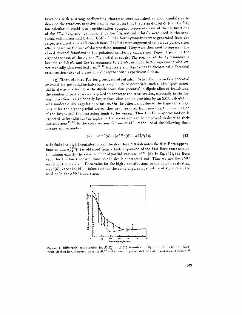
expected to be valid for the high l partial waves and can be employed to describe theircontributions4S -5o to the cross section. Gibson et al. 41 made use of the following Born

closure approximation,

f(O) = a'_BA(o) + [_SM°(0) -- a_(0)]. (42)

to include the high I contributions in the des. Here FBA denotes the first Born approx-

imation and FBAfife (8) is obtained from a finite expansion of the first Born cross section

containing exactly the same number of partial waves as crSMC(o). In Eq. (42), the Bornvalue for the low l contributions to the des is subtracted out. Thus we use the SMC

result for the low l and Born value for the high 1 contributions to the des. In evaluating

o'FBAIO'_FEt, 1, care should be taken so that the same angular quadrature of km and k_ areused as in the SMC calculation.

', T

!2s

!'t L,ii, ,, ,l,JihlJ,,,l, ,,,ltL, _

30 60 go 120 150 180

Scattering ang4e (deg)

Figure 4. Differential cross section for 1 + __.BIX Eg E+ transition of H2 at 15 eV. Solid line, SMCresult, dashed line, distorted wave result, 4s and crosses, experimental data of Srivastava and 3ensen. 4°

343

10

at_

o

at

t

1

i

I I I I |

30 60 90 120 150 180

Scattering angle (deg)

Figure 5. Differential cross section for XlB_ --, BtE_+ transition of H2 at 20 eV. Solid fine, SMCresult, dashed line, distorted wave result,4s crosses, experimental data of Srivastava and Jensen, 4° andtriangles, experimental data of Khakoo and Trajmar. 5°

Equation (42) has been applied to a two-channel SMC calculation to study the1 +

dipole allowed transition X1E + _ B E,, in H2. Figures 4 and 5 present the 15 and 20eV dcs from the SMC calculation with Born closure, the distorted wave calculation of

Rescigno et al., 51 and the experimental data of Srivastava and Jensen s2 and Khakoo

and Trajmar. 53

It should be pointed out that in their implementation of the Born closure approxi-

mation to study elastic scattering of polar molecules, Rescigno et al. 4.54 took a slightly

different approach and apphed it to the body-frame T-matrix instead of the dcs.

3.5. Evaluation of the Green's Function Matrix Elements

The Green's function matrix element

M = (_(_-)IVG(_+)VI%+)),

can be expressed as

M = Mn + i Mr.

The imaginary part MI is given by the residue,

i

.-F. j(43)

where l sums over the poles of G(p+). Since G(p+) is a projected Green's function, this is

equivalent to a sum over the open channels and k, is just the wave vector associated with

the open channel 1. Also, (StlVI_(,, +)) is the same matrix element used in the expression

of the body-frame T-matrix, Tt,,. The integration over l_t in Eq. (43) can use the same

quadrature as the body-frame T-matrix. Consequently, the calculation of MI involves

very little extra work.

The real part of M is given by the principal-value integral,

1 [oo k Um_MR: (_) 3"pJo dc _ (E-C,) _ + i_"

IEopen

(44)

344

with

Vm,,(k) -- J d_:(_-)lVl¢/k="+')(e'k="*''_dVl_+)), (45)

1 2Here e = _k . Due to the integration over _ and 1_, MR is much more difficult to

compute. Its efficient and accurate calculation is an important factor in the development

of a practical SMC method. Two approaches to computing this integral are described

below.

(a) Direct numerical calculation over a quadrature of 1_ and e. An opti-

mized quadrature is obviously important in this approach. To avoid the rapid variation

of the integrand in the e coordinate near the poles of the Green's function, we follow

the work of Waiters 5s and Heller and Reinhardt 5s and separate the _-integration into

two regions, with the poles of the Green's function all located in the first region. The

rapid variation in the first integrand is avoided by the addition and subtraction of a

term such that the numerical integration can be carried out over a smooth integrand.

The e-integral in the first region is rewritten as,

11 _ T, fo', kU,-,,,,(k) de{ kUm,,(k) k,U,,,,,(kl) k, Um,_(k,!-- deE_E,_e- E fo'"lEopen IEopen

(46)with e_ > (E - Et) for all I. In Eq. (46), the second and third term in the integrand are

obtained from the first by replacing k and k with kt and kt. Because Umn(kz) and kt are

independent of _, the last integral on the right-hand side of Eq. (46) can be evaluated

analytically and Eq. (46) is rewritten as,

,,o - ,,, E --E--, E 7-,j ,

Since the first and second term in the e-integand above have poles at the same place, the

large changes in the integrand near the pole region are canceled out and the integrand

remains smooth, suitable for numerical integration.

To demonstrate the convergence of the numericM quadrature scheme, we calcu-

lated the elastic scattering of CO in the static-exchange approximation, using an SCF

target at the experimental equihbrium geometry. A Gaussian basis, with 5s3pld con-

tracted functions at each nuclear center, represented the continuum electron. The SMC

cMculation included up to l_= = 6. Born closure was not included since our purpose

was to demonstrate the convergence of the VG(+)V quadrature, and the introduction

of a constant correction term from the Born closure would not affect our conclusions.

Also, all calculations used the Gauss-Legendre quadrature.

Figure 6 presents the partiM integrM cross section for e-CO elastic scattering. A

(20x20) quadrature was used for the angular integration and a 20-point quadrature for

the second region , integral. Three different quadratures were used for the first ¢ region,

20, 82, and 48 points. The three cross section curves virtually coalesce, indicating a well

converged result.

The cross section is much more sensitive to the quadrature used in the second ¢

integration. Figure 7 shows the cross sections obtained using 20, 32, and 48 quadrature

points for the second region integration and keeping the other quadratures constant.

Note that the peak of the cross section curve at _ 3.5 eV, arising from the 211 shape

resonance in CO, is shifted to a lower energy when a larger quadrature is used. Also, the

32- and 48-point calculations have similar resonance positions, but the cross sections

themselves differ by _ 10% at the peak.

345

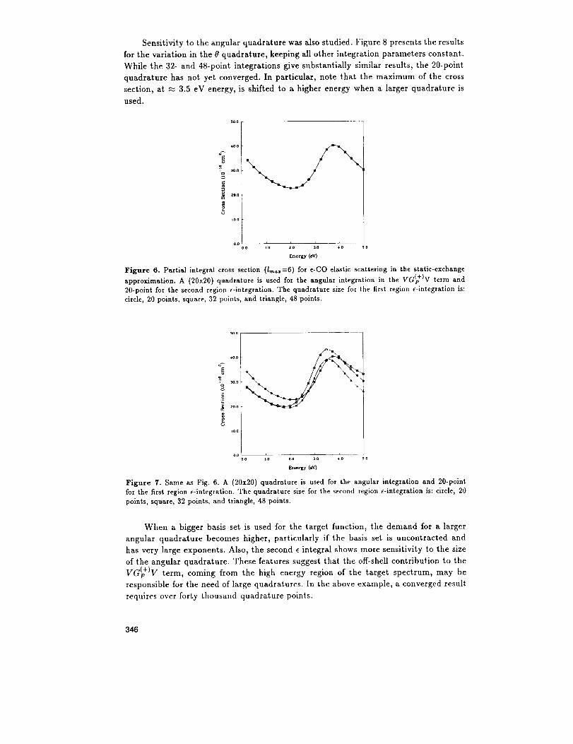
Sensitivity to the angular quadrature was also studied. Figure 8 presents the results

for the variation in the _ quadrature, keeping all other integration parameters constant.

While the 32- and 48-point integrations give substantially similar results, the 20-point

quadrature has not yet converged. In particular, note that the maximum of the cross

section, at _ 3.5 eV energy, is shifted to a higher energy when a larger quadrature is

used.

o_

oooo 1o zo 30 40 _0

Energy (eV)

Figure 6. Partial integral cross section (l,,_ffi=6) for e-CO elastic scattering in the static-exchange

approximation. A (20x20) quadrature is used for the angular integration in the VG(+)V term and

20-point for the second region e-integration. The quadrature size for the first region e-integration is:circle, 20 points, square, 32 points, and triangle, 48 points.

300oC

_ zouL

10o

oo too i.o z.o 30 40 _ o

EnerlLV (eV)

Figure 7. Same as Fig. 6. A (20x20) quadrature is used for the angular integration and 20-pointfor the first region e-integration. The quadrature size for the second region e-integration is: circle, 20

points, square, 32 points, and triangle, 48 points.

When a bigger basis set is used for the target function, the demand for a larger

angular quadrature becomes higher, particularly if the basis set is uncontracted and

has very large exponents. Also, the second e integral shows more sensitivity to the size

of the angular quadrature. These features suggest that the off-shell contribution to the

VG(p+)V term, coming from the high energy region of the target spectrum, may be

responsible for the need of large quadratures. In the above example, a converged result

requires over forty thousand quadrature points.

346

+0 0

E

ic_ 3o o

20Om

p

10a

oooo io ,_o 30 40 _o

Energy (eV)

Figure 8. Same as Fig.6. A 20-point quadrature is used for the first region c-integration, 48 for thesecond, and 20 for the _ integration. Circle, 20-poln¢ 0 quadrature, square, 32 points, and triangle, 48

points.

Tile direct numerical integration approach was first investigated by Lima el al. sr

To expedite the integral calculation, Winstead et al. ss have successfully adapted the

integral calculation and the three-index transformation s/ to the highly parallel com-

puters. Parallel computers are particularly well suited for this purpose because each

integral calculation is independent of others. SMC calculations using this technique

have been carried out on many polyatomic moleculesJ 2

(b) Insertion using a Gaussian basis. Provided that a Caussian basis satisfies

the approximate relation

a

the free-particle Green's function can be projected into this basis, called the insertion

basis. The principal-value Green's function matrix element is now written as

1-- pb(rN+_)lV _ )

lCopen b

× P/o _ d_ / dl_k (p_(rN+,)Ic_krN+_ I@ 'k'rN+*[Pb(rN+,)) (47)(E- _)- _+i_

Both _ and 1<integrals are expressed in closed form. 59 Furthermore, calculations of these

Gaussian integrals are an order of magnitude faster than the three-Gaussian-one-plane

wave integrals in Eq. (45).

It is important to recognize that in Eq. (47), an L 2 basis is used in the evaluation

of an integral over the Green's function, but not to represent the Green's function itself.

Just as an L 2 basis can be used to represent a trial function in a Schwinger variational

calculation because the trial function is always multiplied by V in the expression of

the T-matrix, in the present case the free-particle Green's function is integrated over

VIii'(+)), with the trial _(+) itself expressed in terms of another L 2 basis. Thus, the

long range oscillatory part of the Green's function does not contribute to the integral.

In this respect, the application of an L 2 basis to evaluate MR is analogous in spirit to

s' The fourth index is the plane wave.

347

Schneider's calculation 6° of the Schwinger separable potential by projection onto an L _

basis.

The insertion technique was used in early SMC calculations when large, uncon-

tracted Gaussian bases were used for the scattering basis, with the insertion basis

usually composed of the scattering basis supplemented by additional Gaussians. Good

convergence behavior was observed. 39 The change to the direct numerical integration

technique by Lima et al.s7 was motivated by the convergence problems they encoun-

tered. Such problems appeared to be related to choosing a suitable insertion basis.

In view of recent progress made in the field of quantum chemistry in developing

flexible Gaussian bases, 33 and the efficiency in the computation of Gaussian integrals

themselves, we re-investigated the insertion technique. 2° The choice of a suitable basis

was guided by the convergence characteristics observed in the numerical integration

approach, namely that the off-shell high energy contribution to MR seems to play an

important role in the convergence. To describe this type of contribution, we included

Gaussians with large exponents. Also, a multicentered Gaussian basis readily simulates

the dependence on the angular quadrature. When the insertion basis was chosen using

these guidelines, good convergence was observed. As an example, we studied the e-CO

static-exchange problem using the same scattering basis as discussed above. The inser-

tion basis is obtained by supplementing the scattering basis by 10slSpgd Gaussians at

each nuclear center and 16sSpgd Caussians at the center of mass. 6/Figure 9 compares

the cross sections obtained using the insertion method versus the direct numerical in-

tegration approach. Good agreement is observed. The largest discrepancy between the

two results, less than 3%, is found at the low energy region. In the 2II shape resonance

region, the two curves almost coalesce.

_0

3o0o

20.O

to.o

o.o o,o l.o z.o 3.0 4.0 _ 0

Eneru (eV')

Figure 9. Partial integral cross section (lmaffi=6) for e-CO elastic scattering in the static-exchangeapproximation. Square, calculated using a direct numericM integration, and circle, calculated with the

insertion technique. The numerical integration uses a (32x32) angular quadrature, 20-point for the firstE integration, and 48-point for the second. The insertion basis is described in the text.

While the insertion basis used for the CO calculation appears to be very large, it

should be pointed out that the insertion basis has 238 Gaussian functions and the total

number of Gaussian integrals used is 15.2 million. The numerical integration calculation

6/ Not all components of the d functions were used. Also, a smaller size p_ basis was used at thenuclear center.

348

requires more than 2.78 billion three-Gaussian-one-plane wave type integrals. 7/ Taking

into account the difference in the cycle time required to calculate the two types of

integrals, the insertion technique requires orders of magnitude less CPU and storage

resources.

Recently, Bettega et al.61 apphed the pseudopotential method and removed the

core electrons from the SMC calculations. This raises an interesting question. Since the

off-shell high energy contribution to MR that we observed originate, at least partially,

from the core electrons, the use of pseudopotentials may lessen the demand for large

quadratures in the numerical integration technique and the demand for tight Gaussians

in the insertion technique. This aspect remains to be tested.

3.6. Correlated Target Function in the SMC Method

Because molecular bonding changes with nuclear geometry, multiconfiguration

wave functions are required to provide a consistent description of the target over a

range of geometries. Similarly, the description of several electronic states with a com-

mon set of orbitals, a practice frequently used in the study of electronic excitations

by electron or photon impact, requires the use of multiconfiguration target functions.

Thus correlated target functions are used with some frequency in ab initio studies of

e-molecule collisions, s2-6s

An ubiquitous feature in the use of multiconfiguration target functions is the pres-

ence of pseudoresonances at intermediate energies. 62' 6s Lengsfield and Rescigno 62 at-

tributed these resonances to the fact that multiconfiguration target functions can in-

troduce certain terms in the N + 1-electron wave function which are associated with

excited states of the target excluded from the open channel space. Pseudoresonances

appear at an energy where the excited target state becomes open. Consider the example

of a two-configuration function for the ground state of H2 s/

_x = al¢l + a2¢2,

with

¢1 = A{laga(1)lag_(2)},

¢2 = A{la_a(1)Xa_fl(2)}.

Here _x is the simplest function that can describe the dissociation of It2 properly.

Two N + 1-electron CSF's are used to relax the orthogonality between the target

and the continuum electron,

O_ = AN+,{Ox(1,2)I_,a(3)}

and

Ob = .AN+I { OX(1,2)la,_O_(3) )

= a2.AN+l{¢2(1,2)lago_(3)}.

= alAN+l{¢l(1,2)la,,a(3)).

Here .AN+I antisymmetrizes electron 3 with electrons 1 and 2. Note that ®, includes the

terms 1_%a(1)lm, a(2)la=fl(3) and laga(1)la,,_(2)la,,a(3). These terms are associated

with the b3_ + target state, with the la,, orbital representing the continuum electron. In

the Kohn calculation it was found that if the 3 +b E, state was not included in the open

7/ As a result of symmetry operations, in both eases the actual number of distinct integrals to be

calculated are less. However, the ratio of the the two numbers will be approximately the same when

symmetry is taken into account.

s/ This example was originally used by Lengsfield and Reseigno. 4' 62

349

channel space, a pseudoresonance would occur around the energy where this channel

became open. Similar pseudoresonances were also observed in the R-matrix calculation

of the electronic excitations of H2. ss The strategy used in the Kohn method to eliminate

such terms has been discussed. 4' 62

Due to the use of the N-electron projection operator, the SMC method treats corre-

lated target functions differently. As seen in Sec. 3.1, the N-electron projection operator

selects the terms that are associated with the target function from an antisymmetrized

N + 1-electron CSF, resulting in an un-antisymmetrized product of the N-electron

target function and an one-electron orbital describing the continuum electron. For a

multiconfiguration target function, this operation has additional consequences. As an

illustration, consider the same two-configuration wave function. The projection operator

P is given by

The operation of P on ®a gives,

PiOo) = a2_(I)x (1, 2)lager(3).

Thus the operation of P recovers the _ba component in Oa, originally eliminated by

antisymmetrization. In this manner, the projector P removes the b3E + character from

O_, and POa, unlike O_ itself, consists only of the open channel target.

In an SMC calculation, a pseudoresonance usually appears when the denonfinator

in the expression of the T-matrix becomes particularly small at a certain energy. Because

Oo includes a term that behaves like a open channel function, the matrix element

(@(-)l,qlOo),

as a function of energy E goes through a minimum around the energy when that channel

becomes open. On the other hand, P®_ does not have any ba_ + character, and

(_(-)lgPlOo),

does not exhibit the same minimum.

Based on this analysis, an SMC calculation is expected to perform differently from

other methods when a multiconfiguration target is used. Figure 10 presents an SMC

study of the 2_g+ channel elastic scattering of H2, using the static-exchange approxima-

tion. The calculation was carried out at R = 4.0 ao, using a Gaussian basis of 6s6p at

H and 4s4p at the center of mass, The CI coefficients of the two-configuration target

function are 0.8785 and -0.4778. As seen in Fig. 10, the SMC cross section curve is

smooth over the energy range of 0.25 to 21 eV. The pseudoresonance found in other

methods, arising due to the term ®a, is absent here. Thus it appears that the role of

the projection of P on ®o is to associate ®o with the correct open channel, and thereby

removes the spurious resonance.

The above results suggests that the N-electron projection operator has additional

advantages besides providing a convenient treatment for exchange. The use of correlated

target function in the SMC method is relatively recent. Only a few studies have been

made using a multiconfiguration target function. 22 Future studies should explore this

aspect further.

35O

.!....EnerlD" (ev)

Figure 10. Integral cross section for e-H2 2_+ channel elastic scattering in the static-exchange ap-

proximation, calculated using a two-texm CI function for the target

4. THE USE OF SMC RESULTS IN THE STUDY OF VIBRATIONAL

EXCITATIONS

All SMC calculations use the fixed-nuclei approximation. However, the fixed-nuclei

SMC results can be readily used as a starting point in the application of the nuclear

dynamics treatment of Domcke. Domcke's treatment, which is based on the projection

operator formalism, has been reviewed recently, _3 and it will not be repeated. Here

we consider an example of combining the two approaches in the study of the resonant

enhanced vibrational excitation of N2 by electron impact. Because the 2Ha resonance

in N2 is a pure d-wave resonance, we rewrite the T-matrix for the l=2 partial wave in

terms of the K-matrix,

K(E,R)

T,=2(E, R) = 1 - iK(E, R) '

where R is the internuclear distance. The K-matrix element is related to the width

V(E, R) and shift A(E, R) functions by

r(E,R)

K(E, R) = - 2[E - ed(R) - A(E, R)] "

Here ed is the difference between the target and negative ion potential curves. The shift

function is given by the principal value integral,

A(E,R)= 17) f dE, F(E',R)27r J E - E' '

and the width function can be expressed in terms of the potential Ud_ which Domcke

called the entry amplitude,

F(E, R) = 2_IVdEi 2.

An analytical fit of UdE can be obtained using the K-matrix determined from the SMC

calculation. Notice that Uds is a nonlocal potential, depending on both R and E.

The calculation on N2 has been reported previously. 3° ss In applying Domcke's

method, we used a Schwinger-type separable potential approach to evaluate the T-

matrix element. A complete set of the bound vibrational wave function of the transient

351

negative ion, obtained using a numerical solution of the 1-d schr/_dinger equation, was

used in the separable potential calculation. The negative ion curve was determinedempirically by Berman et al.s7

The results of this calculation compared well with experiment, and the comparison

will not be repeated. Here we consider an example of applying our result to an experi-

mentally inaccessible region. In very high temperature plasmas, as in the flow field of a

high-speed space vehicle upon entry to the earth's atmosphere, molecules are very hot

ro-vibrationally and it is difficult to duplicate such conditions in the laboratory. Figure

11 presents the v = 0 _ 1 and v = 3 _ 4 vibrational excitation cross sections of N_

by electron impact. While many experimental measurements on transitions from v = 0

have been done, there has been only one reported measurement with the initial state at

the v = 1 level. 6s Due to the difficulties involved in preparing a significant quantity of

N2 at the v = 3 level, no measurement has been reported for excitations from this level

and theoretical data is the only available source for these cross sections. It is seen from

Fig. 11 that the resonance structures for the v = 3 --* 4 transition is more extended

both at high and low energies in comparison with the v= 0 --* 1 transition, and not as

strongly peaked. The calculation assumed the molecule was initially at J = 50, with the

centrifugal barrier in the vibrational potential determined by this J value. Note that

our calculation did not include rotation in the dynamics and the effect of rotation only

entered through the centrifugal term.

e.o

Ii 403.o

z.o

t o -. ,,,/

o.ot.a z.o 3.o 4.0

Electron EnerlLy (eV)

Figure 11. N2 vibrational excitation cross sections by electron impact. Solid line, v = 0 --* 1, dashed,v = 3 ---, 4. The cMculation assumes the molecule is at J -- 50.

Figure 12 presents the v = 0 --* 1 excitation cross sections for N2 at d=0, 50, and

150. Again rotational effects contribute only through the centrifugal barrier of vibra-

tional motion. Because the differences between the potential curves of the neutral and

transient negative ion, the large centrifugal barriers at J = 50 and 150 have differentialeffects on the vibrational excitation. The resonance structure in the cross section moves

to lower energies and narrows as d increases.

Future studies that couple vibrational and rotational motion at high d will extendour understanding of the collisional processes involving ro-vibrationally hot molecules.

352

o

I

,o

to,o

o l_b li

e_o _ i iI IpI i I

i L i _bI i h r _

4_o - _ I_ PlI I Jlb I h_l I r_

L LI q2_o i _ I

i i

a.o 3 o _o

Electron Energy (ev)

Figure 12. N2 v : 0 -_ 1 vibrational excitation cross section by electron impact. Solid line, J = 0,dotted, J--50, and dashed, J= 150.

5. SUMMARY

The SMC method, a modified version of the SV method, has proven to be a ver-

satile tool in the study of e-molecule collisions. The SMC method has been successfully

applied to the study of technologically important electron collision processes involving

polyatomic targets. This application will continue as the SMC method is further devel-

oped and refined. The present discussion of its implementation also serves to illustrate

some of the physical basis in its formulation, and provides a foundation for the future

development of the method.

References

1 L. Hulth6n, Kgl. Fysiograf. S/iJbkap. Lund. FrSh. 14,257 (1944).

2 W. Kohn, Phys. Rev. 74, 1763 (1948).

3 S.I. Rubinow, Phys. Rev. 96,218 (1954).

4 T.N. Rescigno, C.W. McCurdy, A.E. Orel, and B.H. Lengsfield III, "The Complex Kohn

Variational Method," chapter 1 in this book.

s J.L. Jackson, Phys. Rev. 83,301 (1951).

R.K. Nesbet, Variational Methods in Electron-Atom Scattering Theory, Plenum Press,

New York (1980).7 B.I. Schneider, "An R-Matrix Approach to Electron Molecule Collisions," chapter 8 in

this book.

s j. Schwinger, Phys. Rev. 56,750 (1947).9 R.R. Lucchese, K. Takatsuka, and V. McKoy, Phys. Rep. 131,147 (1986).

lo D.K. Watson, Adv. At. Mol. Phys. 25,221 (1988).

11 M.A.P. Lima, T.L. Gibson, L.M. Brescansin, V. McKoy, and W.M. Huo, "Studies of

Elastic and Electronically Inelastic Electron-Molecule Collisions," in Swarm Stud-

ies and Inelastic Electron-Molecule Collisions, ed. L.C. Pitchford, B.V. MeKoy, A.

Chutjian, and S. Trajmar, Springer-Verlag, New York (1987), pp 239-264.

12 C. Winstead and V. McKoy, "Studies of Electron-Molecule Collisions on Highly Parallel

Computers," in Modern Electronic Structure Theory Vol. _, ed. D. Yarkony, World

Scientific, Singapore (1994).

353

13 D.K. Watson and V. McKoy, Phys. Rev. A 20, 1474 (1979).

14 R.R. Lucchese, G. Raseev, and V. McKoy, Phys. Rev. A 25, 2572 (1982).

ls See, for example, G. Bandarage and R.R. Lucchese, Phys. Rev. A 47, 1989 (1993);

M.-T. Lee, K. Wang, and V. McKoy, J. Chem. Phys. 97, 3108 (1992).

16 M.-T. Lee, M.M. Fujimoto. S.E. Michelin, L.E. Machado, and L.M. Brescansin, J. Phys.

B. 25, L505 (1992).

17 M.-T. Lee, S.E. Michelin, L.M. Brescansin, G.D. Meneses, and L.E. Machado, J. Phys.

B. 26, L477 (1993).

18 K. Takatsuka and V. McKoy, Phys. Rev. A 24, 2473 (1981).

19 K. Takatsuka and V. McKoy, Phys. Rev. A 30, 1734 (1981).

20 W.M. Huo and J.A. Sheehy (to be published).

21 C. Winstead, Q. Sun, and V. McKoy, J. Chem. Phys. 97, 9483 (1992).

22 W.M. tiuo and J.A. Sheehy, "Theoretical Study of Electron Scattering by Small Clusters

and Adsorbates," in Electron Collisions with Molecules, Clusters, and Surfaces, ed.

H. Ehrhardt and L.A. Morgan, Plenum, New York (1994), pp 171-182.

2a W. Domcke, Phys. Rep. 208, 97 (1991).

24 R.G. Newton, Scattering Theory of Waves and Particles, Springer-Verlag, New York

(1982).

28 B.H. Bransden, R. Hewitt, and M. Plummer, J. Phys. B 21, 2645 (1988).

26 S.K. Adhikari and I.H. Slosh, Phys. Rev. C 11, 1133 (1975).

27 K. Takatsuka, R.R. Lucchese, and V. McKoy, Phys. Rev. A 24, 1812 (1981).

28 J.T. Taylor, Scattering Theory, R. E. Krieger Publishing, FL (1983), pp. 274-279.

29 H. Feshbach Ann. Phys. 5. 357 (1958); ibid 19, 287 (1962).

z0 M.A.P. Lima and V. McKoy, Phys. Rev. A 38, 501 (1988).

31 W.M. Huo and C.A. Weatherford, Bull. Am. Phys. Soc. 36, 1265 (1991).

32 C. Winstead and V. McKoy, Phys. Rev. A 47, 1514 (1993).

33 T. Helgaker and P.R. Taylor, "Gaussian Basis Sets and Molecular Integrals" in Mod-

ern Electronic Structure Theory Vol. 2, ed. D. Yarkony, World Scientific, Singapore

(1994).

34 T.H. Dunning, J. Chem. Phys. 53, 2823 (1970).

38 T.H. Dunning, J. Chem. Phys. 90, 1007 (1989), and D.E. Woon and T.H. Dunning, J.

Chem. Phys. 98, 1358 (1993).

36 As an example of valence excitation calculations which neglected Rydberg states in the

open channel configurations, see Q. Sun, C. Winstead, V. McKoy, J.S.E. Germano,

and M.A.P. Lima, Phys. Rev. A 46, 2462 (1992).

37 W.M. Huo, M.A.P. Lima, T.L. Gibson, and V. McKoy, Phys. Rev. A 36, 1642 (1987).

38 B.H. Lengsfield, T.N. Rescigno, and C.W. McCurdy, Phys. Rev. A 44, 4296 (1991).

z9 W.M. Huo, T.L. Gibson, M.A.P. Lima, and V. McKoy, Phys. Rev. A 36, 1632 (1987).

4o A.J.R. da Silva, M.A.P. Lima, L.M. Brescansin, and V. McKoy, Phys. Rev. A 41, 2903

(1991).

41 T.L. Gibson, M.A.P. Lima, V. McKoy, and W.M. Huo, Phys. Rev. A 35, 2473 (1987).

42 N.S. Ostlund, Chem. Phys. Letters, 34,419 (1975).

43 W.M. Huo and J.A. Sheehy (to be published). See also J.A. Sheehy and W.M. Huo,

"Low-Energy Elastic Electron Scattering from Carbon Tetrafluoride" in ICPEAC

354

AbstractsVol.I, ed.T. Andersen, B. Fastrup, F. Folkmann, H. Knudsen, (1993),

p. 259.

44 C. Winstead, Q. Sun, and V. McKoy, J. Chem. Phys. 98, 1105 (1993).

4s W.M.Huo, Phys. Rev. A 38, 3303 (1988).

46 A. Mann and F. Linder, J. Phys. B 25,545 (1992).

47 L. Boesten, H. Tanaka, A. Kobayashi, M.A. Dillon, and M. Kimura, J. Phys. B 25,

1607 (1992).

4a D.W. Norcross and N.T. PadiaJ, Phys. Rev. A 25,226 (1982).

49 S. Chung and C.C. Lin, Phys. Rev. A 17, 1874 (1978).

so A.W. Fliflet and V. McKoy, Phys. Rev. A 21, 1863 (1980).

sl T.N. Rescigno, C.W. McCurdy, Jr., and V. McKoy, J. Phys. B 7, 2396 (1974).

52 S.K. Srivastava and S. Jensen, J. Phys. B 10, 3341 (1977). See S. Trajmar, D.F. Register,

and A. Chutjian, Phys. Rep. 97, 219 (1983) for renormallzation of this data.

s3 M.A. Khakoo and S. Trajmar, Phys. Rev A 34, 146 (1986).

54 T.N. Rescigno, B.H. Lengsfield, C.W. MeCurdy, and S.D. Parker, Phys. Rev. A 45,

7800 (1992).

ss H.J.R. Waiters, J. Phys. B 4,437 (1971).

s8 E.J. He[ler and W.P. Reinhardt, Phys. Rev. A 7, 365 (1973).

57 M.A.P. Lima, L.M. Brescansin, A.J.R. da Silva, C. Winstead, and V. McKoy, Phys.

Rev. A 41,327 (1990).

s8 C. Winstead, P.G. Hipes, M.A.P. Lima, and V. McKoy, J. Chem. Phys. 94, 5455 (1991).

_9 D.A. Levin, A.W. Fliflet, M. Ma, and V. McKoy, J. Comp. Phys. 28, 416 (1978).

80 B.I. Schneider, Phys. Rev. A 31, 2188 (1985).

81 M.H.F. Bettega, L.G. Ferreira, and M.A.P. Lima, Phys. Rev. A 47 1111 (1993).

62 B.H. Lengsfield III and T.N. Rescigno, Phys. Rev. A 44, 2913 (1991).

83 T.N. Rescigno, B.H. Lengsfield III, and A.E. Orel, J. Chem. Phys. 99, 5097 (1993).

84 C.J. Gillan, O. Nagy, P.G. Burke, L.A. Morgan and C.J. Noble, J. Phys. B 20, 4585

(1987).

8_ S.E. Branchett and J. Tennyson, Phys. Rev. Letts. 64, 2889 (1990).

88 W.M. Huo, V. McKoy, M.A.P. Lima, and T.L. Gibson, "Electron-Nitrogen Molecule

Collisions in High-Temperature Nonequilibrium Air," in Thermalphysical Aspects of

Re-entry Flows, ed. J.N. Moss and C.D. Sott, AIAA, New York (1986), pp. 152-196.

87 M. Berman,H. Estrada, L.S. Cederbaum, and W. Domcke, Phys. Rev. A28, 1363 (1983).

8s S.F. Wong, J.A. Michejda, and A. Stamatovic, unpublished data.

355