r. w. ericksonecen5797/course_material/... · 2018-10-19 · 20 log 10 f f 0 n 20n log 10 f f 0 f f...

R. W. EricksonDepartment of Electrical, Computer, and Energy Engineering

University of Colorado, Boulder

Fundamentals of Power Electronics Chapter 8: Converter Transfer Functions1

Chapter 8. Converter Transfer Functions

8.1. Review of Bode plots8.1.1. Single pole response8.1.2. Single zero response8.1.3. Right half-plane zero8.1.4. Frequency inversion8.1.5. Combinations8.1.6. Double pole response: resonance8.1.7. The low-Q approximation8.1.8. Approximate roots of an arbitrary-degree polynomial

8.2. Analysis of converter transfer functions8.2.1. Example: transfer functions of the buck-boost converter8.2.2. Transfer functions of some basic CCM converters8.2.3. Physical origins of the right half-plane zero in converters


Converter Transfer Functions

8.3. Graphical construction of converter transferfunctions

8.3.1. Series impedances: addition of asymptotes8.3.2. Parallel impedances: inverse addition of asymptotes8.3.3. Another example8.3.4. Voltage divider transfer functions: division of asymptotes

8.4. Measurement of ac transfer functions andimpedances

8.5. Summary of key points


The Engineering Design Process

1. Specifications and other design goals are defined.2. A circuit is proposed. This is a creative process that draws on the

physical insight and experience of the engineer.3. The circuit is modeled. The converter power stage is modeled as

described in Chapter 7. Components and other portions of the systemare modeled as appropriate, often with vendor-supplied data.

4. Design-oriented analysis of the circuit is performed. This involvesdevelopment of equations that allow element values to be chosen suchthat specifications and design goals are met. In addition, it may benecessary for the engineer to gain additional understanding andphysical insight into the circuit behavior, so that the design can beimproved by adding elements to the circuit or by changing circuitconnections.

5. Model verification. Predictions of the model are compared to alaboratory prototype, under nominal operating conditions. The model isrefined as necessary, so that the model predictions agree withlaboratory measurements.


Design Process

6. Worst-case analysis (or other reliability and production yieldanalysis) of the circuit is performed. This involves quantitativeevaluation of the model performance, to judge whetherspecifications are met under all conditions. Computersimulation is well-suited to this task.

7. Iteration. The above steps are repeated to improve the designuntil the worst-case behavior meets specifications, or until thereliability and production yield are acceptably high.

This Chapter: steps 4, 5, and 6


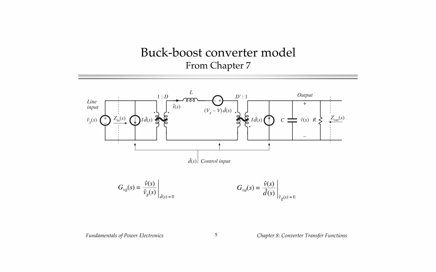
Buck-boost converter modelFrom Chapter 7

+–

+–

L

RC

1 : D D' : 1

vg(s) Id(s) Id(s)

i(s) +

v(s)

–

(Vg – V)d(s)Zout(s)Zin(s)

d(s) Control input

Lineinput

Output

Gvg(s) = v(s)vg(s)

d(s) = 0

Gvd(s) = v(s)d (s) vg(s) = 0


Design-oriented analysis

How to approach a real (and hence, complicated) systemProblems:

Complicated derivationsLong equationsAlgebra mistakes

Design objectives:Obtain physical insight which leads engineer to synthesis of a good designObtain simple equations that can be inverted, so that element values can

be chosen to obtain desired behavior. Equations that cannot be invertedare useless for design!

Design-oriented analysis is a structured approach to analysis, which attempts toavoid the above problems


Some elements of design-oriented analysis,discussed in this chapter

• Writing transfer functions in normalized form, to directly expose salientfeatures

• Obtaining simple analytical expressions for asymptotes, cornerfrequencies, and other salient features, allows element values to beselected such that a given desired behavior is obtained

• Use of inverted poles and zeroes, to refer transfer function gains to themost important asymptote

• Analytical approximation of roots of high-order polynomials• Graphical construction of Bode plots of transfer functions and

polynomials, toavoid algebra mistakesapproximate transfer functionsobtain insight into origins of salient features


Bode plot of control-to-output transfer functionwith analytical expressions for important features

f

0˚

–90˚

–180˚

–270˚

|| Gvd ||

Gd0 =

|| Gvd || �Gvd

0 dBV

–20 dBV

–40 dBV

20 dBV

40 dBV

60 dBV

80 dBV

Q =

�Gvd

10-1/2Q f0

101/2Q f0

0˚

–20 dB/decade

–40 dB/decade

–270˚

fz /10

10fz

1 MHz10 Hz 100 Hz 1 kHz 10 kHz 100 kHz

f0

VDD' D'R C

L

D'2/ LC

D' 2R2/DL(RHP)

fz

DVg

t(D')3RC

Vg

t2D'LC


8.1. Review of Bode plots

Decibels

G dB = 20 log10 G

Table 8.1. Expressing magnitudes in decibels

Actual magnitude Magnitude in dB

1/2 – 6dB

1 0 dB

2 6 dB

5 = 10/2 20 dB – 6 dB = 14 dB

10 20dB1000 = 103 3 ! 20dB = 60 dB

Z dB = 20 log10

ZRbase

Decibels of quantities havingunits (impedance example):normalize before taking log

5! is equivalent to 14dB with respect to a base impedance of Rbase =1!, also known as 14dB!.60dBµA is a current 60dB greater than a base current of 1µA, or 1mA.


Bode plot of fn

G = ff0

n

Bode plots are effectively log-log plots, which cause functions whichvary as fn to become linear plots. Given:

Magnitude in dB is

G dB = 20 log10ff0

n

= 20n log10ff0

ff0

– 2

ff0

2

0dB

–20dB

–40dB

–60dB

20dB

40dB

60dB

flog scale

f00.1f0 10f0

ff0

ff0

– 1

n = 1n =

2

n = –2

n = –120 dB/decade

40dB/decade

–20dB/decade

–40dB/decade

• Slope is 20n dB/decade

• Magnitude is 1, or 0dB, atfrequency f = f0


8.1.1. Single pole response

+–

R

Cv1(s)

+

v2(s)

–

Simple R-C example Transfer function is

G(s) = v2(s)v1(s)

=1

sC1

sC + R

G(s) = 11 + sRC

Express as rational fraction:

This coincides with the normalizedform

G(s) = 11 + s

t0

with t0 = 1RC


G(j!) and || G(j!) ||

Im(G(jt))

Re(G(jt))

G(jt)

|| G(jt

) ||

�G(jt)

G( jt) = 11 + j t

t0

=1 – j t

t0

1 + tt0

2

G( jt) = Re (G( jt)) 2 + Im (G( jt)) 2

= 11 + t

t0

2

Let s = j!:

Magnitude is

Magnitude in dB:

G( jt)dB

= – 20 log10 1 + tt0

2 dB


Asymptotic behavior: low frequency

G( jt) = 11 + t

t0

2

tt0

<< 1

G( jt) 5 11

= 1

G( jt)dB5 0dB

ff0

– 1

–20dB/decade

ff00.1f0 10f0

0dB

–20dB

–40dB

–60dB

0dB

|| G(jt) ||dB

For small frequency,! << !0 and f << f0 :

Then || G(j!) ||becomes

Or, in dB,

This is the low-frequencyasymptote of || G(j!) ||


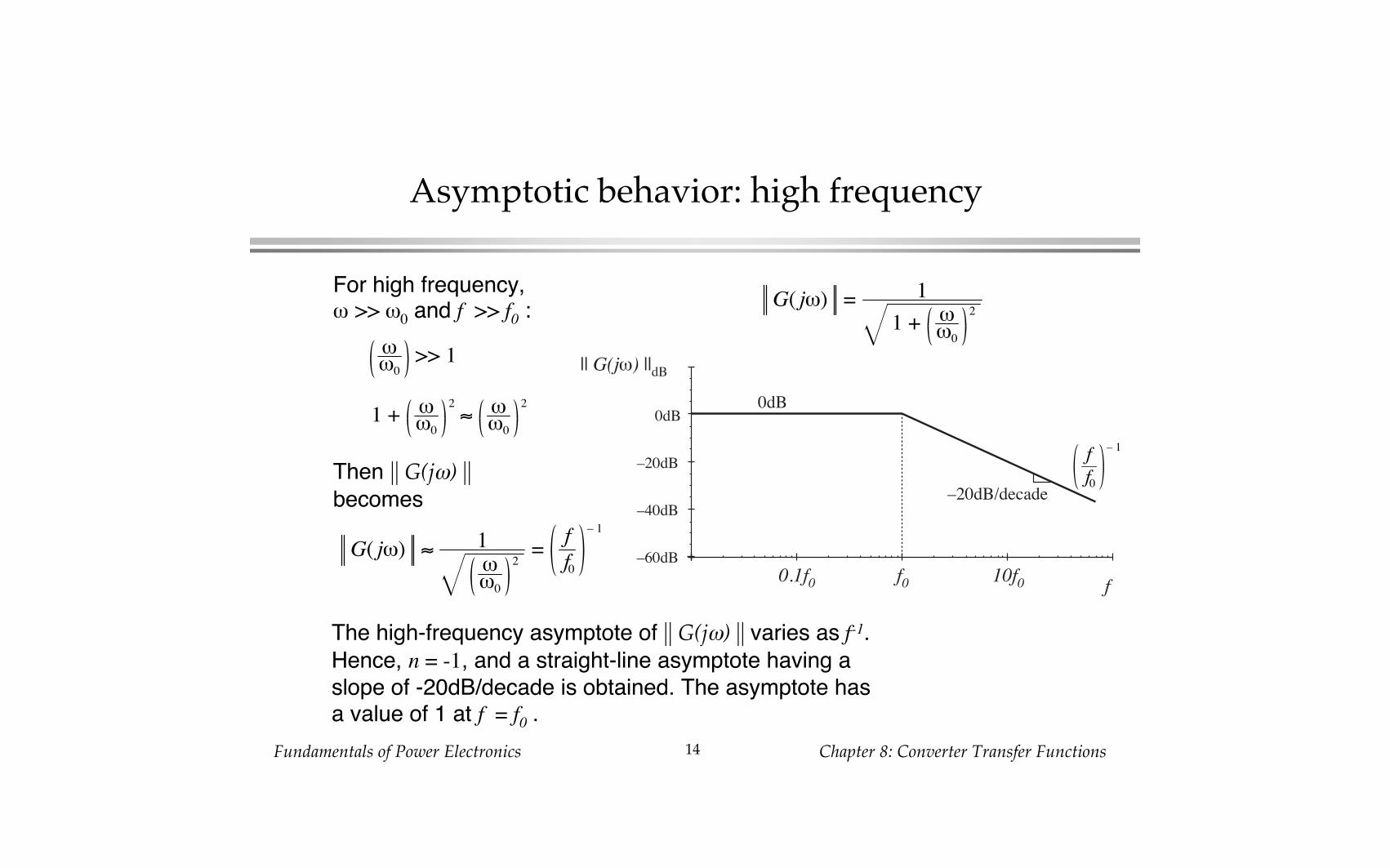
Asymptotic behavior: high frequency

G( jt) = 11 + t

t0

2

ff0

– 1

–20dB/decade

ff00.1f0 10f0

0dB

–20dB

–40dB

–60dB

0dB

|| G(jt) ||dB

For high frequency,! >> !0 and f >> f0 :

Then || G(j!) ||becomes

The high-frequency asymptote of || G(j!) || varies as f-1.Hence, n = -1, and a straight-line asymptote having aslope of -20dB/decade is obtained. The asymptote hasa value of 1 at f = f0 .

tt0

>> 1

1 + tt0

25 t

t0

2

G( jt) 5 1tt0

2= f

f0

– 1


Deviation of exact curve near f = f0

Evaluate exact magnitude:at f = f0:

G( jt0) = 1

1 + t0t0

2= 1

2

G( jt0) dB= – 20 log10 1 + t0

t0

25 – 3 dB

at f = 0.5f0 and 2f0 :

Similar arguments show that the exact curve lies 1dB belowthe asymptotes.


Summary: magnitude

–20dB/decade

f

f0

0dB

–10dB

–20dB

–30dB

|| G(jt) ||dB

3dB1dB0.5f0 1dB

2f0


Phase of G(j!)

G( jt) = 11 + j t

t0

=1 – j t

t0

1 + tt0

2

�G( jt) = tan– 1Im G( jt)Re G( jt)

Im(G(jt))

Re(G(jt))

G(jt)

|| G(jt

) ||

�G(jt)�G( jt) = – tan– 1 t

t0


-90˚

-75˚

-60˚

-45˚

-30˚

-15˚

0˚

f

0.01f0 0.1f0 f0 10f0 100f0

�G(jt)

f0

-45˚

0˚ asymptote

–90˚ asymptote

Phase of G(j!)

�G( jt) = – tan– 1 tt0

! "G(j!)

0 0˚

!0–45˚

# –90˚


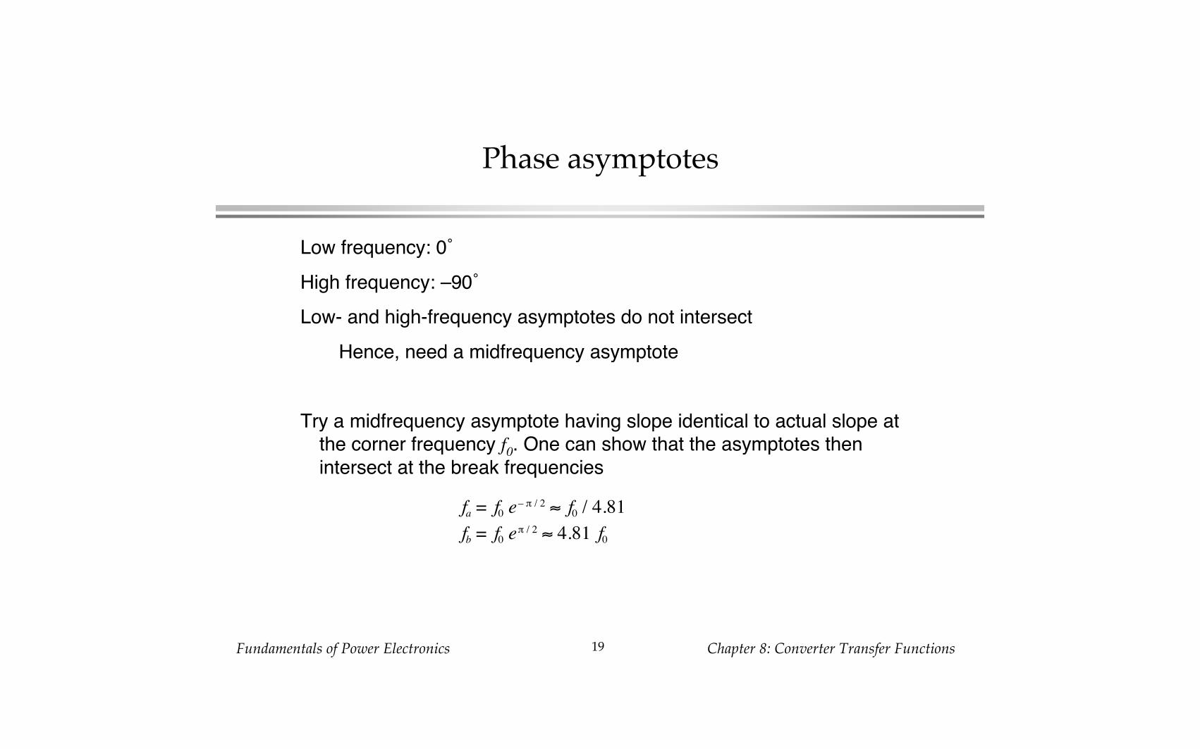
Phase asymptotes

Low frequency: 0˚High frequency: –90˚Low- and high-frequency asymptotes do not intersect

Hence, need a midfrequency asymptote

Try a midfrequency asymptote having slope identical to actual slope atthe corner frequency f0. One can show that the asymptotes thenintersect at the break frequencies

fa = f0 e– / / 2 5 f0 / 4.81fb = f0 e/ / 2 5 4.81 f0


Phase asymptotes

fa = f0 e– / / 2 5 f0 / 4.81fb = f0 e/ / 2 5 4.81 f0

-90˚

-75˚

-60˚

-45˚

-30˚

-15˚

0˚

f

0.01f0 0.1f0 f0 100f0

�G(jt)

f0

-45˚

fa = f0 / 4.81

fb = 4.81 f0


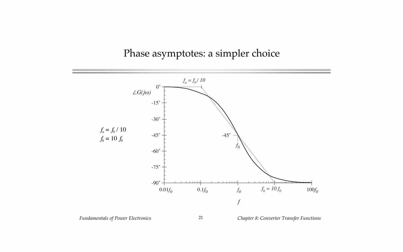
Phase asymptotes: a simpler choice

-90˚

-75˚

-60˚

-45˚

-30˚

-15˚

0˚

f

0.01f0 0.1f0 f0 100f0

�G(jt)

f0

-45˚

fa = f0 / 10

fb = 10 f0

fa = f0 / 10fb = 10 f0


Summary: Bode plot of real pole

0˚�G(jt)

f0-45˚

f0 / 10

10 f0

-90˚

5.7˚

5.7˚

-45˚/decade

–20dB/decade

f0

|| G(jt) ||dB 3dB1dB0.5f0 1dB

2f0

0dB G(s) = 11 + s

t0


8.1.2. Single zero response

G(s) = 1 + st0

Normalized form:

G( jt) = 1 + tt0

2

�G( jt) = tan– 1 tt0

Magnitude:

Use arguments similar to those used for the simple pole, to deriveasymptotes:

0dB at low frequency, ! << !0

+20dB/decade slope at high frequency, ! >> !0

Phase:

—with the exception of a missing minus sign, same as simple pole


Summary: Bode plot, real zero

0˚�G(jt)

f045˚

f0 / 10

10 f0 +90˚5.7˚

5.7˚

+45˚/decade

+20dB/decade

f0

|| G(jt) ||dB3dB1dB

0.5f01dB

2f0

0dB

G(s) = 1 + st0


8.1.3. Right half-plane zero

Normalized form:

G( jt) = 1 + tt0

2

Magnitude:

—same as conventional (left half-plane) zero. Hence, magnitudeasymptotes are identical to those of LHP zero.Phase:

—same as real pole.The RHP zero exhibits the magnitude asymptotes of the LHP zero,and the phase asymptotes of the pole

G(s) = 1 – st0

�G( jt) = – tan– 1 tt0


+20dB/decade

f0

|| G(jt) ||dB3dB1dB

0.5f01dB

2f0

0dB

0˚�G(jt)

f0-45˚

f0 / 10

10 f0

-90˚

5.7˚

5.7˚

-45˚/decade

Summary: Bode plot, RHP zero

G(s) = 1 – st0


8.1.4. Frequency inversion

Reversal of frequency axis. A useful form when describing mid- orhigh-frequency flat asymptotes. Normalized form, inverted pole:

An algebraically equivalent form:

The inverted-pole format emphasizes the high-frequency gain.

G(s) = 11 + t0

s

G(s) =st0

1 + st0


Asymptotes, inverted pole

0˚

�G(jt)

f0+45˚

f0 / 10

10 f0

+90˚5.7˚

5.7˚

-45˚/decade

0dB

+20dB/decade

f0

|| G(jt) ||dB

3dB

1dB

0.5f0

1dB2f0

G(s) = 11 + t0

s


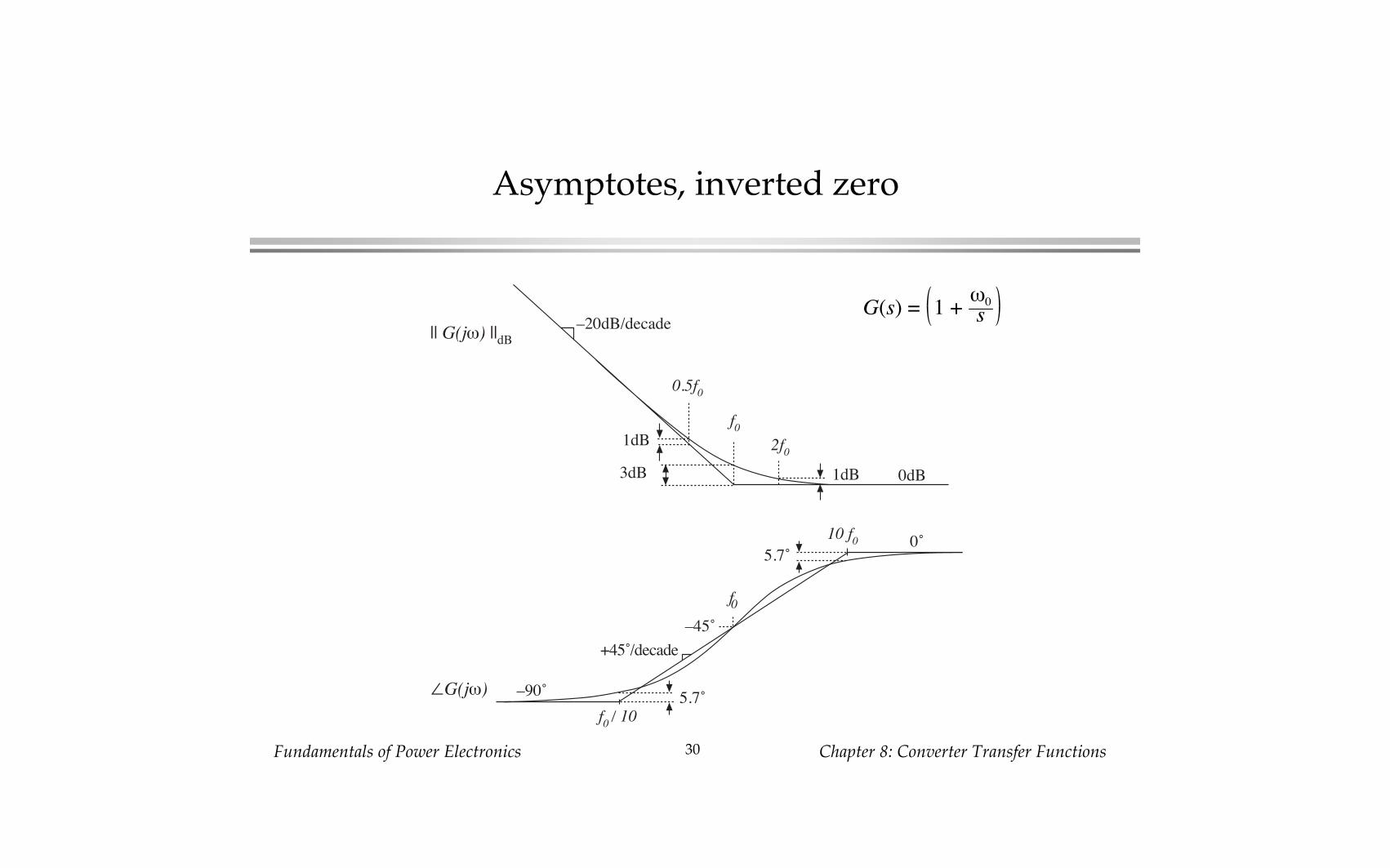
Inverted zero

Normalized form, inverted zero:

An algebraically equivalent form:

Again, the inverted-zero format emphasizes the high-frequency gain.

G(s) = 1 + t0s

G(s) =1 + s

t0

st0


Asymptotes, inverted zero

0˚

�G(jt)

f0–45˚

f0 / 10

10 f0

–90˚

5.7˚

5.7˚

+45˚/decade

–20dB/decade

f0

|| G(jt) ||dB

3dB

1dB

0.5f0

1dB

2f0

0dB

G(s) = 1 + t0s


8.1.5. Combinations

Suppose that we have constructed the Bode diagrams of twocomplex-values functions of frequency, G1(!) and G2(!). It is desiredto construct the Bode diagram of the product, G3(!) = G1(!) G2(!).

Express the complex-valued functions in polar form:G1(t) = R1(t) e je1(t)

G2(t) = R2(t) e je2(t)

G3(t) = R3(t) e je3(t)

The product G3(!) can then be writtenG3(t) = G1(t) G2(t) = R1(t) e je1(t) R2(t) e je2(t)

G3(t) = R1(t) R2(t) e j(e1(t) + e2(t))


Combinations

G3(t) = R1(t) R2(t) e j(e1(t) + e2(t))

The composite phase ise3(t) = e1(t) + e2(t)

The composite magnitude is

R3(t) = R1(t) R2(t)

R3(t)dB

= R1(t)dB

+ R2(t)dB

Composite phase is sum of individual phases.Composite magnitude, when expressed in dB, is sum of individual

magnitudes.


Example 1: G(s) = G0

1 + st1

1 + st2

–40 dB/decade

f

|| G ||

� G

� G|| G ||

0˚

–45˚

–90˚

–135˚

–180˚

–60 dB

0 dB

–20 dB

–40 dB

20 dB

40 dB

f1100 Hz

f22 kHz

G0 = 40 � 32 dB–20 dB/decade

0 dB

f1/1010 Hz

f2/10200 Hz

10f11 kHz

10f220 kHz

0˚

–45˚/decade

–90˚/decade

–45˚/decade

1 Hz 10 Hz 100 Hz 1 kHz 10 kHz 100 kHz

with G0 = 40 ! 32 dB, f1 = "1/2! = 100 Hz, f2 = "2/2! = 2 kHz


Example 2

|| A ||

� A

f1

f2

|| A0 ||dB +20 dB/dec

f1 /10

10f1 f2 /10

10f2

–45˚/dec+45˚/dec

0˚

|| A' ||dB

0˚

–90˚

Determine the transfer function A(s) corresponding to the followingasymptotes:


Example 2, continued

One solution:

A(s) = A0

1 + st1

1 + st2

Analytical expressions for asymptotes:For f < f1

A0

1 + st1➚

1 + st2➚

s = jt

= A011 = A0

For f1 < f < f2

A0

1➚ + st1

1 + st2➚

s = jt

= A0

st1 s = jt

1 = A0tt1

= A0ff1


Example 2, continued

For f > f2

A0

1➚ + st1

1➚ + st2

s = jt

= A0

st1 s = jt

st2 s = jt

= A0t2t1

= A0f2f1

So the high-frequency asymptote is

A' = A0f2f1

Another way to express A(s): use inverted poles and zeroes, andexpress A(s) directly in terms of A!

A(s) = A'

1 + t1s

1 + t2s


8.1.6 Quadratic pole response: resonance

+–

L

C Rv1(s)

+

v2(s)

–

Two-pole low-pass filter example

Example

G(s) = v2(s)v1(s)

= 11 + s L

R + s2LC

Second-order denominator, ofthe form

G(s) = 11 + a1s + a2s2

with a1 = L/R and a2 = LC

How should we construct the Bode diagram?


Approach 1: factor denominator

G(s) = 11 + a1s + a2s2

We might factor the denominator using the quadratic formula, thenconstruct Bode diagram as the combination of two real poles:

G(s) = 11 – s

s11 – s

s2

with s1 = – a12a2

1 – 1 – 4a2

a12

s2 = – a12a2

1 + 1 – 4a2

a12

• If 4a2 ! a12, then the roots s1 and s2 are real. We can construct Bode

diagram as the combination of two real poles.• If 4a2 > a1

2, then the roots are complex. In Section 8.1.1, theassumption was made that !0 is real; hence, the results of thatsection cannot be applied and we need to do some additional work.


G(j!) and || G(j!) ||

Im(G(jt))

Re(G(jt))

G(jt)

|| G(jt

) ||

�G(jt)

G( jt) = 11 + j t

t0

=1 – j t

t0

1 + tt0

2

G( jt) = Re (G( jt)) 2 + Im (G( jt)) 2

= 11 + t

t0

2

Let s = j!:

Magnitude is

Magnitude in dB:

G( jt)dB

= – 20 log10 1 + tt0

2 dB


Approach 2: Define a standard normalized formfor the quadratic case

G(s) = 11 + 2c s

t0+ s

t0

2 G(s) = 11 + s

Qt0+ s

t0

2or

• When the coefficients of s are real and positive, then the parameters !,"0, and Q are also real and positive

• The parameters !, "0, and Q are found by equating the coefficients of s• The parameter "0 is the angular corner frequency, and we can define f0

= "0/2#

• The parameter ! is called the damping factor. ! controls the shape of theexact curve in the vicinity of f = f0. The roots are complex when ! < 1.

• In the alternative form, the parameter Q is called the quality factor. Qalso controls the shape of the exact curve in the vicinity of f = f0. Theroots are complex when Q > 0.5.


The Q-factor

Q = 12c

In a second-order system, ! and Q are related according to

Q is a measure of the dissipation in the system. A more generaldefinition of Q, for sinusoidal excitation of a passive element or systemis

Q = 2/ (peak stored energy)(energy dissipated per cycle)

For a second-order passive system, the two equations above areequivalent. We will see that Q has a simple interpretation in the Bodediagrams of second-order transfer functions.


Analytical expressions for f0 and Q

G(s) = v2(s)v1(s)

= 11 + s L

R + s2LC

Two-pole low-pass filterexample: we found that

G(s) = 11 + s

Qt0+ s

t0

2Equate coefficients of likepowers of s with thestandard form

Result: f0 = t02/ = 1

2/ LCQ = R C

L


Magnitude asymptotes, quadratic form

G( jt) = 1

1 – tt0

2 2+ 1

Q2tt0

2

G(s) = 11 + s

Qt0+ s

t0

2In the form

let s = j! and find magnitude:

Asymptotes are

G A 1 for t << t0

G Aff0

– 2

for t >> t0

ff0

– 2

–40 dB/decade

ff00.1f0 10f0

0 dB

|| G(jt) ||dB

0 dB

–20 dB

–40 dB

–60 dB


Deviation of exact curve from magnitude asymptotes

G( jt) = 1

1 – tt0

2 2+ 1

Q2tt0

2

At ! = !0, the exact magnitude isG( jt0) = Q G( jt0) dB

= Q dBor, in dB:

The exact curve has magnitudeQ at f = f0. The deviation of theexact curve from theasymptotes is | Q |dB

|| G ||

f0

| Q |dB0 dB

–40 dB/decade

Fundamentals of Power Electronics! Chapter 8: Converter Transfer Functions!45!

Phase asymptotes!

f / f0

�G

0.1 1 10

Increasing Q

–180°

–90°

0°

284 Converter Transfer Functions

At high frequencies where (ω/ω0) > 1, the (ω/ω0)4 term

dominates the expression inside the radical of Eq. (8.62).Hence, the high-frequency asymptote is

(8.64)

This expression coincides with Eq. (8.5), with n = – 2.Therefore, the high-frequency asymptote has slope –40 dB/decade. The asymptotes intersect at f = f0, and are indepen-dent of Q.

The parameter Q affects the deviation of the actualcurve from the asymptotes, in the neighborhood of the cor-ner frequency f0. The exact magnitude at f = f0 is found by substitution of ω = ω0 into Eq. (8.62):

(8.65)

So the exact transfer function has magnitude Q at the corner frequency f0. In decibels, Eq. (8.65) is

(8.66)

So if, for example, Q = 2 ⇒ 6 dB, then the actual curve deviates from the asymptotes by 6 dB at the cor-ner frequency f = f0. Salient features of the magnitude Bode plot of the second-order transfer function aresummarized in Fig. 8.20.

The phase of G is

(8.67)

The phase tends to 0˚ at low frequency, and to –180˚ at high frequency. At f = f0, the phase is –90˚. Asillustrated in Fig. 8.21, increasing the value of Q causes a sharper phase change between the 0˚ and–180˚ asymptotes. We again need a midfrequency asymptote, to approximate the phase transition in the

|| G ||

f0

| Q |dB0 dB

–40 dB/decade

Fig. 8.20 Important features of the magni-tude Bode plot, for the two-pole transferfunction.

G →ff0

– 2for ω> ω0

G( jω0) = Q

G( jω0) dB = Q dB

∠G( jω) = – tan– 11Q

ωω0

1 – ωω0

2

Fig. 8.21 Phase plot, second-order poles.Increasing Q causes a sharper phase change.

f / f0

∠G

0.1 1 10

Increasing Q

–180°

–90°

0°•  Low frequency asymptote of 0˚"•  High frequency asymptote of

–180˚"•  Change from 0˚ to –180˚

becomes more sharp as Q is increased"

Fundamentals of Power Electronics! Chapter 8: Converter Transfer Functions!46!

Mid-frequency phase asymptote!

f / f0

�G

0.1 1 10–180°

–90°

0°

f0

–90°

fb

fa0°

–180°

f / f0

�G

0.1 1 10–180°

–90°

0°

f0

–90°

fb

fa0°

–180°

8.1 Review of Bode Plots 285

vicinity of the corner frequency f0, as illustrated in Fig. 8.22. As in the case of the real single pole, wecould choose the slope of this asymptote to be identical to the slope of the actual curve at f = f0. It can beshown that this choice leads to the following asymptote break frequencies:

(8.68)

A better choice, which is consistent with the approximation (8.28) used for the real single pole, is

(8.69)

With this choice, the midfrequency asymptote has slope –180Q degrees per decade. The phase asymp-totes are summarized in Fig. 8.23. With Q = 0.5, the phase changes from 0˚ to –180˚ over a frequencyspan of approximately two decades, centered at the corner frequency f0. Increasing the Q causes this fre-quency span to decrease rapidly.

Second-order response magnitude and phase curves are plotted in Figs. 8.24 and 8.25.

fa = eπ/ 2 – 12Q f0

fb = eπ/ 212Q f0

fa = 10– 1/2Q f0fb = 101/2Q f0

Fig. 8.22 One choice for the midfrequencyphase asymptote of the two-pole response,which correctly predicts the actual slope atf = f0.

f / f0

∠G

0.1 1 10–180°

–90°

0°

f0

–90°

fb

fa0°

–180°

Fig. 8.23 A simpler choice for themidfrequency phase asymptote, whichbetter approximates the curve over theentire frequency range and is consistentwith the asymptote used for real poles.

f / f0

∠G

0.1 1 10–180°

–90°

0°

f0

–90°

fb

fa0°

–180°

8.1 Review of Bode Plots 285

vicinity of the corner frequency f0, as illustrated in Fig. 8.22. As in the case of the real single pole, wecould choose the slope of this asymptote to be identical to the slope of the actual curve at f = f0. It can beshown that this choice leads to the following asymptote break frequencies:

(8.68)

A better choice, which is consistent with the approximation (8.28) used for the real single pole, is

(8.69)

With this choice, the midfrequency asymptote has slope –180Q degrees per decade. The phase asymp-totes are summarized in Fig. 8.23. With Q = 0.5, the phase changes from 0˚ to –180˚ over a frequencyspan of approximately two decades, centered at the corner frequency f0. Increasing the Q causes this fre-quency span to decrease rapidly.

Second-order response magnitude and phase curves are plotted in Figs. 8.24 and 8.25.

fa = eπ/ 2 – 12Q f0

fb = eπ/ 212Q f0

fa = 10– 1/2Q f0fb = 101/2Q f0

Fig. 8.22 One choice for the midfrequencyphase asymptote of the two-pole response,which correctly predicts the actual slope atf = f0.

f / f0

∠G

0.1 1 10–180°

–90°

0°

f0

–90°

fb

fa0°

–180°

Fig. 8.23 A simpler choice for themidfrequency phase asymptote, whichbetter approximates the curve over theentire frequency range and is consistentwith the asymptote used for real poles.

f / f0

∠G

0.1 1 10–180°

–90°

0°

f0

–90°

fb

fa0°

–180°Match slope at f = f0:" Choose same approximation as in real pole case:"

or"


Two-pole response: exact curves

Q = '

Q = 5

Q = 2

Q = 1Q = 0.7

Q = 0.5

Q = 0.2

Q = 0.1

-20dB

-10dB

0dB

10dB

10.3 0.5 2 30.7

f / f0

|| G ||dB

Q = 0.1

Q = 0.5Q = 0.7Q = 1Q = 2Q =5Q = 10Q = '

-180°

-135°

-90°

-45°

0°

0.1 1 10

f / f0

�G

Q = 0.2

r. w. ericksonecen5797/course_material/... · 2018-10-19 · 20 log 10 f f 0 n 20n log 10 f f 0 f f...

Documents