BROWN UNIVERSITYPROVIDENCE, R. I.

MODE APPROXIMATIONS FOR IMPULSIVELY LOADED

RIGID PLASTIC STRUCTURES

BY

J. B. TIN and P. S. SYMONDSFR CLEA 7NGH U37F. .F ANDfiardc-y- j icrok c. N

__--r~, . N7 C!ML.: ON,-np;

•ai T49•eoc MWodel SBa%•c,U4,d~reva4' E 14•&a, ?C4ca ,4 ""'Cc'(. g

.•~ ~ e 0' 0[i Q, 0. A)<

MMODE APPROXIMATIONS FOR

IMPULSIVELY LOADED RIGID-PLASTIC STRUCTURES

by

1 2J. B. Martin and P. S. Symondsz

Summary:

An attempt is made to provide a rational method of constructing

one degree of freedom approximations for impulsively loaded metal

structures which are analysed according to an elementary rigid-plastic

theory. The approximation follows automatically from a chosen mode

shape, and a criterion for determining good mode shapes is introduced.

'Assistant Professor of Engineering, Brown University.

2Professor of Engireering, Brown University.

4 A

I1. INTRODUCTION

The problem of the estimation of permanent deformations in ductile met

structures subjected to high intensity dynamic loading has received increasing

I attention over the past fifteen years. The problem is, in its entirety, one of gre

difficulty. Above the complexity of the problem of elastic structures subjected ti

g transient loading, additional complicating factors which are of importance includ

i the dissipation of energy in plastic work, elastic unloading from plastic states, N

hardening, the dependence of yield stress upon rate of strain, geometry change (

I and divers other non-linear effects. Very few solutions to dynamic loading prob:

have recognized all these factors. More commonly, one or i iore of the factors

assumed to dominate the behavior of the structure, and all others are neglected

I approximated.

Probably the most widely used approximation3 is the replacement of the

distributed mass of the structure by one or more point masses. This approxima

has been used in conjunction with a variety of idealizations of the material behav

J In fairly simple structurcs the actual distribution of mass, elastic stiffi

and yield stress can be considered. Solutions for an elastic, perfectly plastic

S 3 See, for example:

N. M. Newmark, "A method of computation for structural dynamics," Proc. EMech. Div., A. S. C. E., 85, (EM3), p. 67, 1959.

C. H. Norris, et al. Structural Design for Dynamic Loads, McGraw-Hill Bootj Co., New York, N. Y., 1959.

iI

-2-

material have been but are difficult if the load magnitudes are much larger

than those causing the yield stress to be reached. A variety of dynamic loading

problems has been solved using what will be termed in th.is paper an elemenrta~ry

rigid-plastic theory. A representative but by no means complete list of papers is5

given. The elementary rigid-plastic theory involves the following idealizations:

(i) For the purpose of the dynamic loading problem under consideration

a ductile material is represented by a rigid, perfectly plastic constitu-

tive equation. All elastic effects are in consequence excluded.

(ii) Geometry changes are assumed to be small, and the yield stress is

assumed to be independent of the rate of strain.

4For example:

H. H. Bleich and M. G. Salvadori, "Impulsive motion of elasto-plastic beams,Trans. A.S.C.E., IZ0, p. 499, 1955.

J. A. Seiler, B. A. Cotter, and P. S. Symonds, "Impulsive loading of elastic-plastic beams," J. App. Mech., 23, p. 515, 1956.

5 E. H. Lee and P. S. Symonds, "Large plastic deformations of beams undertransverse impact," J. App. Mech., 19, p. 308, 1952.

M. F. Conroy, "Plastic-rigid analysis of long beams under transverse impact,"J. App. Mech., 19, p. 465, 1952.

P. S. Symonds, "Dynamic load characteristics in plastic bending of beams,"J. App. Mech. , 20, p. 475, 1953.

H. G. Hopkins and W. Prager, "On the dynamics of plastic circular plates,"z. angew. Math. u Phys., 5, p. 317, 1954.

E. W. Parkes, "The permanent deformation of a cantilever struck transverselyat its tip," Proc. Roy. Soc., A228 , p. 462, 1955.

P. G. Hodge, Jr. , "Impact pressure loading of rigid-plastic cylindrical shells,"J. Mech. Phys. Sol., 3, p. 176, 1955.

-3-

The use of the elementary rigid-plastic theory is the subject of this paper.

It is not within the scope or the report, however, to give a complete appraisal of

the utility and applicability of this theory. It.is entirely a valid method of approach,

as are the other idealizations mentioned above, provided that care is taken to define

the range where idealization and reality have something in common, and provided

that experimental evidence confirms the theoretical predictions it. this range. The

elementary rigid-plastic theory, when applied to structures subjected to short

duration, high intensity loading, has a range of validity bounded at one end by the

requirement that the deformations should not be so large that geometry change

effects are significant, and at the other end by the requirement that the energy of th,

disturbance should be large compared to the energy which could be stored elasticall

in the structure in order to justify the exclusion of elastic effects. These require-

ments are in some senses contradictory since the large disturbance needed to meet

the energy requirement will tend to produce large deformations. Thus the extent

of the possible range of validity of the elementary rigid-plastic theory must depend

on the configuration and flexibility of the structure, and in some cases may not exis

at all.

Experiments show that the rigid-plastic theory almost always requires

corrections for the dependence of yield stress on strain rate, strain hardening and

geometry changes. When these corrections are made, remarkably good agreement

-4-

6has been achieved , showing that the neglect of elastic effects is permissible when

the total energy dissipated is much greater than maximum energy which could be

stored elastically. 'a appropriate circumstances it is possible to make the

corrections for strain rate sensitivity and for strain hardening by simply multiplying

the static yield stress by a constant factor 7; however, the "appropziate circumstance

are not always obvious, and this method should be used with caution for a highly rate

sensitive material such as mild steel.

In the authors' opinion the importance of the elementary rigid-plastic theory

lies in its ability to provide, quickly and simply, an estimate of major deforrrations

due to very large dynamic loads. Such an estimate provides a convenient basis for

more refined analyses and calculations to include effects of strain rate sensitiity,

finite deflections, and other effects when necessary.

6S. R. Bodner and P. S. Symonds, "Experimental and theoretical investigation of

the plastic deformation of cantilever beams subjected to impulsive loading,J. App. Mech., 29, p. 719, 1962.

E. H. Lee and S. J. Tupper, "Analysis of plastic deformation in a steel cylinderstriking a rigid target," J. App. Mech., 21, p. 63, 1954.

T. J. Mentel, "The plastic deformation due to impact at a cantilever beam withan attached tip mass," J. A. M., 25, p. 515, 1958.

T. C. T. Ting and P. S. Symonds, "Impact of a cantilever beam with strain ratesensitivity," Proc. Fourth U. S. Nat. Congr. App. Mech., A. S. M. E.,p. 1153, 1962.

A. J. Frick and J. B. Martin, "The plastic deformation of a bent cantilever,"Tech. Rept. NSF GPI115/16 from Brown University to the NationalScience Foundation, April 1965.

7 E. W. Parkes, "The permanent deformation of a cantilever struck transvel sely atits tip," Proc. Roy. Soc., A 228, p. 462, 1955.

I-5-

IThis report will be limited to the discussion of one dimensional coni

i i.e., structures made up of bars and rods, curved or straight, whose cross

I dimensions are small compared with their length. Generalized stresses (bel

moments, axial force, etc.) and generalized strains (curvatures, axial strai

I will be used in the analysis. The following description of the plastic flow ru]

I rigid-perfectly plastic material follows Prager.8

Let the generalized stresses acting at a section be!Q. (j 1,..., n)IJ

and let the associated generalized strain rates beI(j n).

The dimension of a particular component of generalized strain is such that t!

stress-strain product has the dimension of work per unit length. Tift: stress

relation is written in terms of a yield function 4 (Qj) which must be convex a

which must contain the origin. The generalized strain rates are given in ter

the generalized stresses as follows:

1 4q. > ~ (. I

I where

<'(Q) >= 1 when I(Q 0

8 W. Prager, An Introduction to Plasticity. Addison Wesley Press, (ReadinjMassachusetts), 1959.

-6-

< • (Q) > = 0 when t (Q < 0

)X > 0 but otherwise unspecified.

Stresses such that

4 (Q) >0

are not admitted.

The geometric interpretation of equation (I) is now well known. If the r

components of the stress Q. are plotted as coordinates in an n dimensional space3

a stress point is defined. Similarly the convex function * = 0 may also be plott,

as a closed surface in the stress space. If the stress point lies inside the surfac

t = 0, the strain rate is zero. If the stress point lies on the surface, the magnit

of the strain rate vector is not specified. However, if 4 . is plotted in the stress

space with the stress point as origin, the strain rate vector is required to have t

direction of the exterior normal to the surface O= 0 at that point. A two diment

representation of this interpretation is given in Fig. I.

This geometrical approach demonstrates that if Q. is any other admisJ

state of stress (Fig. 1), then

(Q. - Q. )4. >0 (2)

Further, if Q. itself lies on the yield surface and is associated with strain rate

JJqji (shown in Fig. 2), it is clear that by a second application of the concept

deomonstrated in equation (2),

(Q, - Q, )(4. - > )>o (3)

3. 3i 3 3-|

-7-

These inequalities have been discussed in a more general context by Hill9 and

Drucker. 10

Inequality (3) may be used to show that the velocity history at any point

in a structure following the application of high intensity time dependent loading is

unique, provided that changes in geometry may be ignored arid that ce" tain continuity

11requirements are satisfied. This result has been discussed by Martin , and is

12based upon earlier work by Drucker which appears to have passed unnoticed by

most workers in this field.

Suppose that a given structure is subjected to the following loading and

boundary conditions: On length ST of the body time dependent tractions T.T 1

(i = 1, 2, 3) are specified, and on the remainder of the structure S time dependentu

velocities u*. are prescribed. S Tand S , which together comprise the whole

structure, may themselves be time dependent. Further, let the velocities at time

t = 0 be given by v.. These quantities define the problem. Assume now that two1

solutions can be found. First, velocities ii. associated with accelerations *.1 1

9 R. Hill, "A variational principle of maximum plastic work in classical plasticity,"Quart. J. Mech. App. Math., 1, p. 18, 1948.

1 0 D. C. Drucker, "A more fundamental approach to stress-strain relations,"Proc. 1st U. S. Congr. App. Mech., A.S.M.E., p. 487, 1951.

J. B. Martin, "A note on the uniqueness of solutions for dynamically loaded

rigid-plastic and rigid-visco-plastic continua," Tech. Rept. NSF GPI 115/12from Brown University to the National Science Foundation, September 1964.

1 2 D. C. Dr icker, "A definition of a stable inelastic material," J. App. Mech. , 26,j.. 101, 1959.

-8-

resses Q , strain rates_4.. Secondly, velocities u.Z accelerations u. , stresses

strain rates q. . Both solutions satisfy all the field equiations.

Consider the two solutions at sor.nie timE' t >t . Since the tractions, inertia

*ces and stresses of each solution are in internal and external equilibrium, the

.ferences in these quantities are in equilibrium. Similarly, the differences in the

main rates and velocities are compatible. Further, the difference in the tractions

nishes on STo and the difference in displacements vanishes on S . In consequence,U

)m the pritnciple of virtual velocities,

I m• •* .'*S 1 *(cJ•J

m) dS (Q - ) (q- )dS (4)i T ST

.ere m is the mass per unit length of the structure. Froe, (3), the right-ard sidc

non-negative. Hence, provided that the velocity at eaLh point is a continuous

iction of time, we may write

d ( *) 00dt mT i ) ( u ) dS <0 (5)

is seen that a non-negative quantity involving the velocities i., ui . must decre-as',1 1

th time. At time t = 0, however, u. = '. v., and the non-negative quZntity isI ~1

tially zero. It follo, . that u. = u. for all t > 0.1 1

The restriction imposed by the requirement that the velocity at each point

ould be a continuous function of time is a serious one in general. It may readily

shown that when discontinuities are permitted thŽ solutions to certain problems are

-9-

not unique (Ting 1). In practice, however, a large class of problems where

discontinuities do not occur is of interest. This is the class of structural problems

where shear and axial strains are stipulated zero (bending and torsion strains are

permitted). The velocity at each point will be a continuous function of time in these

cases, and hence uniqueness follows. This report will be restricted to problems

falling into this class.

Further, the report will be concerned only with impulsive loading problems.

These problems may be characterized in exactly the same way as the general

problem given above with the following restrictions:

(i) The tractions applied to ST will be taken to be zero.

(ii) The velocities prescribed on S will be taken to be zero.u

(iii) S and ST will be assumed to be time independent.

The impulsive loading problem is thus essentially one in which initial velocities are

prescribed over the whole structure at time t = 0; thereafter, no external forces do

work on the structure.

No direct technique exists for determining the response of the structure to

this (or any other more complex) form of loading. A solution must be sought on a

trial and error basis. If a solution can be found which satisfies all the conditions

(equilibrium, compatibility, yield and the stress-strain relation), the uniqueness

result assures that this is the only solution for the velocity as a function of space

and time.

13 T. C. T. Ting. Private communication., March 1965.

-10-

The response of a one-dimensional rigid-plastic structure to impulsive

)ading is characterized by two distinct phases of behavior. In the first phase,

!avelling "hinges" (discrete points at which plastic deformation occurs) associated

ith discontinuities in the acceleration field are found. In the second phase, deforma-

on occurs without change of shape of the velocity field. The eq-.ations of the second

hase may be written in terms of separate functions of time and space p'srameters,

nd hence are easily formulated.

14In considering the elementary rigid-plastic solutions, Symonds emphasized

iat in certain cases very simple closed form solutions of impulsive loading problems

an be obtained, for example by momentum conservation equations in finite form.

15xamples were gi 'en where slightly modified problems required numerical irtegra-

.on of the equations. Further examples have been given in the literature. Thus the

roblem of a mass striking a fixed end beam was solved in closed form by Parkes 6

ut for the pin ended case the equations for the first phase have to be solved

17umerically (Ezra ).

4P. S. Symonds, "Large plastic deformations of beams under blast loading,"Proc. Second U. S. Nat. Congr. App. Mech., A.S.M.E., p. 505, 1954.

5 P. S. Symonds, "Simple solutions of impulsive loading and impact problems ofplastic beams and plates," Tech. Rept. UERD-3 from Brown Universityto the Norfolk Naval Shipyard under Contract N1895-1756 A, April 1955.

6E. W. Parkes, "The permanent deformation of an encastrelbeam strucktrans-,ersely at any point in its span," Proc. Inst. Civ. Engrs. (London),10, p. 266, 1958.

7A. A. Ezra, "The plastic response of a simply supported beam to an impactload at the center," Proc. 3rd U. S. Nat. Congr. App. Mech. , A.S. M.E.p. 513, 1958.

-11-

A further example is given in Fig. 3. This is a fixed end beam subjected to

impulsive loading so that the velocity is v in the region of length b. The complete0

solution can be easily obtained in closed form for any ratio b/f. However, if the

ends are pinned rather than clamped a quite unpleasant numerical solution is require

in order to obtain the three quantities required to define the motion in the first phase

This example will be discussed later in the paper.

Although the solution by numerical integration of a problem of elementary

rigid-plastic theory is almost certain to be much less difficult than the solution of

the same problem according to elastic-plastic theory, it may be tedious enough so

that, for purposes of first estimates at least, one would welcome a simple approxim

method. Such methods have frequently been used. The most common method is

equivalent to the replacement of the structure by a mass-spring system of one degre

of freedom. Matching the model to the actual problem has been done in various ad

hoc ways. No attempt seems to have been made to generalize or systematize the

various approximate methods.

This report will discuss a technique of approximation which is closely

related to the matching of one degree of freedom models. Using an argument akin

to that used to establish uniqueness, it will be shown that the solution to one impulsi,

loading problem may be approximated by the solution of a problem involving the sam

structure but different initial velocities.

To make use of this property we shall first give, for illustrative purposes,

the solutions to two simnple problems, and then show how approximations may be

constructed for these and other problems. Finally, we shall discuss the relation

between the two approaches to approximation, showing that the concepts of the previ(

" ' -12-

paragraph may be used to provide a rational method of matching one degree of

freedom models to the structure.

-13-

Z. SOME EXAMPLES OF SIMPLE SOLUTIONS

In this section we shall present two problems which can be very simply

I solved with a rigid-plastic theory. These solutions are given primarily to illustr

problems where the solution for the first phase, when travelling hinges occur, ca

I written in closed form

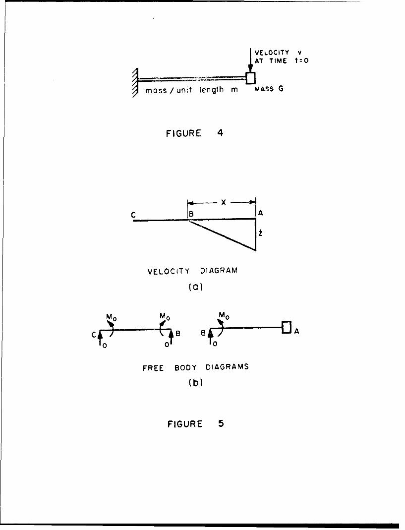
g (i) The first problem considered will be the uniform contilever subjected to

transverse impulse on a point mass attached at the tip. The solution to this prob

7was obtained by Parkes . The beam, with the relevant physical parameters, is

I shown in Fig. 4. At time t = 0, the tip mass acquires a velocity v. Shear strai

are neglected in the analysis, and hence the bending moment is constrained to be

I between +M and -M for all shear force values.0 0

In accordance with the trial technique for solution, a response is postula

and then checked. An assumed velocity field at time t > 0 is shown in Fig. 5(a).

I The sectionAB of the beam rotates about B, and thus the bending moment at B m

j be zero. BC remains stationary, and thus for equilibrium of BC [Fig. 5(b)] the s

force in BC must be zero and the bending moment must be M . Certainly this0

distribution of velocity and strain rate is kinematically admissible, and the stres

j .strain relation has been satisfied.

We give the solution obtained by Parkes7 by writing conservation of

I momentum equations for the beam. Since no external forces act on the beam the

linear momentum of the beam cannot be changed: hence at time t

G 2x. =Gv (6)

I

-14-

Angular momentum about a line through A perpendicular to both the beam center line

and the direction of motion will be considered. The initial angular momentum about

this line is zero; hence at time t

( M t (7)

These equations give • and t in terms of the parameter x. Introducing the dimension-

less parameters

r = rml/ZG ,x/

(6) and (7) become

(Z) Iz •.) = (8av+T• (Ba)

M 0to I e(

Gty - 3 (l + -yt) 8b)

t increases monotonically tto give increasing t, and the solution remains valid until

S= I or the hinge reaches C . Thereafter the beam rotates as a rigid body about C ,

and the behavior enters the second phase. the shear force at C iE no longer zero;

however, angular momentum about C gives a relation between 1 and t directly:

M t -- T-- Gv({ + 2,= Y) ?G +v - Gz- (I +' Of (9)

o 3 (1 +'r) 0 (( ()9)

Rearranging

Mt 0 2-- -) (I + r ) (10)

Giv 3

-15-

This relation applies until i 0.

The equations derived here can be shown to lead to a distribution of bendin

moments which at all times satisfies the yield condition, and hence this is the

solution to the problem. A closed form solution for the final displacement 8 of the

tip mass may be obtained by integrating the tip velocity equations:

M6 20 . = I + log (I + (11)

1 2 3(l+ y) 3yGiv

(ii) As a second cxample, consider a uniform beam subjected to impulsive

loading over a length b symmetric about the midpoint, so that the initial velocity is

v on this section and zero in the remaining length (I - b) [Fig. 6(a)]. The yield0

condition is taken to be the same as that in the previous example. For b = I the

solution was given by Symonds for clamped end and pin end conditions 1 4 ' 15 In

that case it is not difficult to obtain solutions in closed form. In practice, if the

ends are constrained against axial motion, the effects of the constraints tend to

dominate when the deflection exceeds magintudes of the order of the beam depth.

18These effects have been considered8, but they lie beyond the scope of the present

discussion.

For b/I < I, if the ends are built in a closed form solution can be simply

derived. Fig. 6(c) indicates the trial velocity configuration for an instant soon

after motion begins. The sections AP and QC have zero shear force and bending

moment -M and M , respectively. The plastic boundary points are at0 0

1 8 P. S. Symonds and T. J. Mentel, "Impulsive loadings of plastic beams with axial

constraints," J. Mech. Phys. Sol., 6, p. 186, 1958.

x = •I (t)I

and

x 2•(t)I

and these define the motion in this stage. They can be found by writing the two

equations of momentum conservation, namely of linear momentum and angular

momentum about any point in AP or QC. Omitting details, the following results

are found:

2 2 = 12 Mt

(1

0

This stage ends when the hinge at P reaches the support point or that at Q reaches

the midpoint. If b < 1/2, the subsequent stage involves the pattern shown in Fig. 6(d),

the unknown quantities defining the motion now being the midpoint velocity v(t) and

l(t). 1Momentum equations enable us to find these as follows:

= b + 12 1 3a)

1 41 mbiv0

4v 48M t0 = 3 + 0 (13b)

mb v0

These equations hold for times t such that

48 M trn20 <21-3 (14)

mb vb0

-17-

IThe latter time corresponds to the instant when the hinge at P reaches end A of t1

r beam. The two stages treated above comprise the first phase of the motion.

In the second phase there are stationary plastic hinges at A and C. Eac.

half beam rotates as a rigid bar. The midpoint velocity v is found, by writing an

I angular momentum equation, to be given by

21 6 48 M (t

2 v =b 2b 0 mbv

The beam comes to rest when t = tf , where

48 Motf 61of -6-- (16)

mb zv0

The deflections in the various stages are easily found by integrating the velocities

written above. The result for the final midpoint displacement is

S~mb vo 1 .1 .1

Uf =lZ M 4 2In + 1], b 2< (17)0

The three terms show respectively the contributions from the three stages of mot:

Throughout the above analysis the yield condition is everywhere satisfied

Since the equations of dynamics, the boundary conditions and the initial velocity

distribution are all satisfied, the result is the exact solution (according to the

elementary rigid-plastic theory). The above results apply for

I 2b/1 < 1

-18-

A similar analysis for

Zb/I >. I

gives the result

mb2v 2uf - 8 " - 31 (18)_ _ Io b± -

Uf 48 M b b'3](8

When the ends of the beam are pinned rather than built in, the solution for

general b/I < I cannot be obtained in ti-e simple manner used above. The velocity

pattern and free body diagram for the first stage are shown in Figs. 7(b) and 7(d).

These enable the initial velocity conditions and all other requirements to be satisfied.

There are now four unknowns; in addition to t and kz the velocity vI at the hinge

point P and the reaction force RA nmust be found. The four equations in these

unknowns can be written in various ways and will be omitted here. Velocities are

continuous at the hinge points P and Q, but the accelerations are not. The numerical

integrations required to obtain the complete solution are tedious. They have been

carried through for b/I = 0. 2 and b/I = 0. 7.

The two examples given show just how easily some solutions in the elemental

rigid-plastic theory may be obtained. The case discussed in the previous paragraph

shows, on the other hand, how a small change in initial or boundary conditions may

enormously complicate the analysis. Th,. need for a simpler way of obtaining an

approximation to the complcte solution in such cases is apparent.

1 9 G. Gangopadhyay. M. Sc. Thesis, Brown University, 1964. Further calculationson this problem have been carried out by K. Vashi.

-19-

3. ONE DEGREE OF FREEDOM APPROXIMATIONS

A one degree of freedom model appropriate to a rigid-plastic material is

shown in Fig. 8(a). The spring force-spring displacement characteristic is as

shown in Fig. 8(b); essentially motion of the mass is resisted by a constant force S

If the spring is initially undeformed and has initial velocity %P it is clear that the

velocity i, at time t is given by

G'i= Gi - St for >00

or

U St U--- = I - for . > 0 (19)u "Oi u -0 0 0

Thus the velocity of the mass decreases with time, coming to rest in time tf = G~i

The final displa ement is

u = - G o_/sf 2 0

In order to apply these resuits to, for example, a beam problem, suitabh(

values must be found for the quantities L, S and G. These quantities may be refer

to as the equivalent velocity, equivalent resisting force and equivalent mass

respectively.

Consider, for example, the beam shown in Fig. 9(a). This case was

discussed in detail in t1e previous section. A one degree of freedom approxirnatio

will be given for this example in order to demonstrate a method of finding the

equivalent quantities.

-20-

In the case of the spring (Fig. 8) the limiting value of the resisting force

may be found by statically applying an external force to the spring and finding the

value of the external force required to initiate flow. This external force and the

resisting force will havy equal magnitudes. This simple i'.ea provides one mcans i

finding an equivalent force: Apply static loading to the beaam and take the limiting

value of the load parameter as the equivalent resisting force.

In this case choose the loading pattern shown in Fig. 9(b). Only half the

beam is shown because of the symmetry of the system. Statics shows that the

limiting value of P is given by

8MP = ... (20)c 21-b

Steady flow will occur in the beam when P reaches P . The flow field associatt'dc

with P suggests itself as a reasonable means of choosing the equivalent velocity;c

when impulsive loading is applied, it will be assumed that the velocity field has th

same shape as the velocity field s1 own in Fig. 9(c). (Notice that the velocity field

for steady flow under loads P is not unique. The field given is a possible con-c

figuration). It remains, therefore, to determ'ne the amplitude of the velocity fiel<.

as a function of time.

One method of determining the acceleration is to write the angular

acceleration equation for half the beam about the hinge support. If ui and 'd are

the velocity and acceleration of the center of the beam,

3 ,.ml 4 -2M (21)

0

-21 -

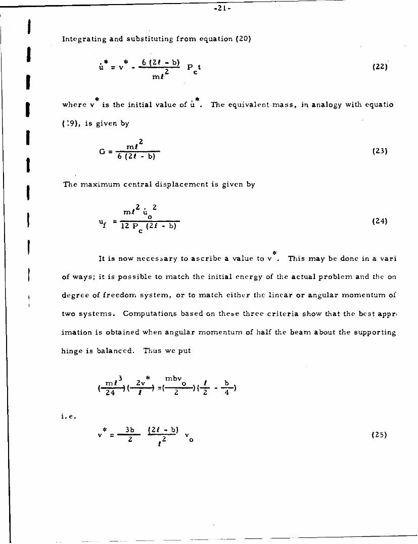
1Integrating and substituting from equation (20)

I .* * 6 (21 - b) (22)u =V ml 2 Pct(2II where v is the initial value of u . The equivalent mass, in analogy with equatio

(':9), is given by

I mt 2

G l6(1-b) (23)

The maximum central displacement is given by

ml 2 i 2I om 124

I Uf 12 21b (24)uf=12 P c(21 - b)C

It is now necessary to ascribe a value to v This may be done in a vari

of ways; it is possible to match the initial energy of the actual problem and the on

degree of freedom system, or to match either the linear or angular momentum of

two systems. Computations based on thebe three criteria show that the best appr,

imation is obtained when angular momentum of half the beam about the supporting

hinge is balanced. Thus we put

3 2v* mbvo

24 H(-• = 2 )(7{ 4

i.e.

v 3b 21 - b)(25)2 1 2 0

Substituting into (24) and rearranging in the form given in equation (18), the

approximato central displacement is given by

, b22 2

* mnb v0 9 (21 -b) 12o 9 12 b'2'(26)

uf 12 M 3 72- 20 1

The derivation of this expression involves many separate decisions which

appear natural but are also arbitrary. If the method is to be applied to find approx-

imate solutions of problems which have not been fully solved it is desirable that the

application of the method should require fewer arbitrary decisions. A more

sophisticated approach using the principle of virtual velocities will ,liminate most

of these decisions.

This method is based on the premise that the choice of a mode shape is

the most important part of the approximation process. Suppose that, for a given

structure, the solution is assumed to be of the form

;j. (S, t) = Si (S) T (t) (27)

where S. is a vector valued function of the space variable S alone, and T is a scalar1

function of time alone. Solutions of this form will be referred to as mode solutions.

Some freedom is permitted in arranging the magnitude and dimensions of the

functions S. and T. For convenience we shall assume that T is dimensionless and1

that it has the value unity when t = 0. S. will thus have the dimensions of velocity;1

it will in fact be the initial velocity distribution. For simplicity in solution we shall

write (27) as

u. (S, t) =v. i(S) T (t) (28)1 1

-23-

If the solution to an impulsive loading problem is to be assumed to be of

the form of (28) it is clearly desirable that v. (S) should satisfy the kinematic1

boundary conditions.

We shall show first that T(t) must be a linear function of time if the intern

energy dissipation rate associated with the assumed velocity field is to be equAl to

the rate of change of kinetic energy. The rate of dissipation of Lhe kinetic energy

K is given by

dK d m .*.*------ ----- • ---- 1u. . dS77t dt S 2 U i, d

d 2 *= dt (T) v. dS

dT C' *

= -T--- m v* v. dS (29)dT dt

The strains q4. may be derived from the velocities u. Let the initial values of.1-

these strains, derived from v. be q •. These strain quantities will be related in

the same way as the velocities

.* Iq -=q T (30)

When the strain component q. is plotted as a vector in the stress space (as in Fig.

it is clear that q. cnanges only in magnitude as t.me progresses. It is, however,

the direction of q. which determines the associated stress vector Q. * (Althoughmy n

0. may not always be uniquely determined, the dissipation rate is unique for aJ

* *given 4. .) Thus Q. does not change with time, and the dissipation rate D is givenJJ

by

D =-Q q. =Q. qT T (31)

where qD . 4. is the initial dissipation rate.

We now equate the rate of change of kinetic energy and the rate of change

of internal energy, given by the total energy dissipation rate with a negative sign.

dT i* * I

T-dT mv. v. dS -T 5 dS1dt

Si dS

dT i S (32)

dt J m v.v. * dSSS I I

X is a constant, defined by (32), which can be readily de ermined from the initial

velocity distribution. Solving equation (32) for T, with the requirement that T = I

when t = 0, we obtain

T = (I - Xt) (33)

The time tf which elapses before motion in the assumed mode ceases is given

simply by

* It =- (34)

It is still necessary to determine the initial velocity field v. since only

the mode shape and not the initial amplitude has been assumed. Suppose that a mode

Ishape f. is assumed. Then

v i =ae. (35)I

and it is necessary to choose the amplitude a. The actual initial velodity distri

will be taken to be v..I

A rational method of determining a may be developed by assuming that

one degree of freedom model is subjected, *at time t = 0,'to an impulse distribul

mv., where m is the mass per unit length of the structure. The velocity with w1

the model begins to move may be then taken to be v.

This problem may be handled by means of the principle of virtual veloc

0. is a kinematically admissible time independent velocity field. Let the assoc:1

strain rates be Suppose now that the model is subjected to forces P. which

over the time interval 0 :< t <-. , causing acceleratioas i. and stresses Q.. For

in the interval

P. O.dS - n-i 0 dS Q dQ. (36)I

SS I I I j

Integrate from time t = 0 to t = -r . Let the initial velocities of the model be ze

and the final velocities v.1

fS 0 Pidt 4i dS = S mvy 4 .dS + dt j" Q.4,dS (37)

Advantage has been taken of the fact that 0. is time independent. We now suppc

1!

that t--0 and that

'•P. dt --*iv. .

0

v. becomes the initial mode velocity and the term of the right of (37), representingI

a measure of work done in the time interval, will vanish. Finally

mv. t.dS= my. I.dS (38)

Substituting from (35) this expression may be written either as

mv.v. dS= my. v. dS (39a)S 1S

or

mv.f.dS

Sm. i4t. dS 139b)

S $~d

Thus, referring back to equation (28), the velocities for a mode solution cal

be written in terms of an initial velocity field agnd a time function; the time function

[ equations (33) and (34)] and the initial velocity field can be determined completely

in terms of an assumed mode shape 4'. and the physica* properties of the structure.1

The application of this method will be illustrated by the case of the beam

shown in Fig. 9. Assume a mode shape of the same form as shown in Fig. 9(c) i. e.

-27-

Iof the same form as was used in the previous approximation. Thus 0 is given 1

2x 0 5 x < 1/2 (40a

I Iand

I v* 2x* O*~ /---- 2 0 e. X -< 1/2 (40b

1 0

The initial conditions for the actual problem (Fig. 9a) are given byIV 1--0 0 <x1<(I - b)/Z

(41)

I v i--v0 (1 - b)/2Sx' 1 ,/Z

I To determine Uo we use equation (39b). This gives

I 1//z

2 my (-- dxJI - 0

0" 22U m( 2x-)2 dx

0zI°I - vb (2 - b) (42)

-- 2 2II

Comparing this result with equation (25), it is seen that the process carried ou

I is equivalent to matching the initial angular momentum of half the beam. The I

I method has an advantage, however, in that it may be easily applied in situation

angular momentum cannot be clearly understood. The time tf which elapsesII

the model comes to rest is given by substitution into equations (32) and (34)

J / 2x 2 *2, 2 f m -.-..- (u ° 0

"24M 2 1

0 mlvb 28 M [ (43)

0

The initial velocity at the center of the beam is u 0 and this velocity changes

linearly with time. Hence the central displacement of the model is given by

* U0 tfu f = 2

2 2mb

)2 2 9-~ mbv b2(44)

=1 M 16(2 - --

Comparing this result with equation (26) which gives the displacement obtained from

the earlier model, we find that the second approximation is twice as large as the

first. This is a substantial difference. Without consulting the correct answer

given in f2 of the paper, we would expect the second result to be more reliable

than the first, since i" involves fewer decisions on the behavior of the model.

However, this is not necessarily true. Further, the choice of a mode shape itself

is an arbitrary decision. Alternative mode shapes for the problem under discussio

-29-

are shown in Fig. 10. It may be possible that these shapes would give better

approximations than Fig. 9(c), at least for certain values of b/1.

If the technique used to obtain the second approximation is to be uhcful in

problems where the exact answer is not known, some method must be found which

can differentiate between a good choice of mode shape and a poor choice. In the

following sections we shall attempt to show how the ideas used in establishing

uniqueness for the problems under discussion can be used to make such a differenti

-30-

4. CONVERGING SOLUTIONS

Using an argument closely related to that used to prove uniqueness, a rela-

tion between the solutions to two independent impulsive loadings (or initial velocity

distributions) on the same structure can be written, provided that the boundary

conditions are the same.

We consider two identical structures with identical boundary conditions (i. e.

velocities prescribed zero on S u, tractions prescribed zero on S T). Let the initial

velocities be respectiv~ely vi (S) and v.* (S), and let the solutions be respectively

U. (S, t), *xi,, 4•, Q.j and u. (S, t), ui. , qj , Q. . As in equation (4), we may write,1- 1 * 1 1 '.' •. 6 J " q3"

S i ) -& )dS Q.-Q. I 4-qj dS> 0 (45

or

dat < 0 (46a)dt -

where

A u ) ( u.. )dS (46b)

The initial value of A , at time t = 0, is given by

0= Mj{v -v. (v. - v )dS (47)Si 1 1 i

It is clear from (46b) tla* t is a non-negative scalar function of time, and, from

-31-I(46a), A decreases with increasing time. The rate of decrease of A is specifiedI *the right hand side of equation (45), and can be zero only when either Q. = Q. or

J J

4.j =qi q. at each point in the structure. Furthermore A is a measure of the differ,

between the two velocity fields ii. and ia., and is zero only when the two fields ar,

identical. According to this measure, therefore, the two solutions approach each

other as time progresses.

The convergence of the two solutions suggests a means of approximating

unknown solution. If the response to the velocities v. are not known, but the resp1

to velocities v. are known, we are assured that the difference between the resporrx(as measured by A ) will decrease with time. If the difference is initially not lari

i.e. if A0 is not large, we may expect that the solutions will not be greatly differ-

particularly away from the initial instants. Furthermore, we would not expect gr

differences in the velocities at any particular point on the structure (as opposed tc

integrated effect represented by A).

These ideas may be applied to attempts to approximate responses by inea

of mode solutions, as discussed in the previous section. However, in order to

substitute a mode solution for u.* in equation (45) it must be a complete solution t(1

an initial valae problem. The mode sol:tions used in the previous section were

required to be kinematically admissible only. If it is possible to associate with th

motle solution a statically admissible stress field which everywhere satisfies the

yield condition, then the mode solution is a full solution to an initial value problerr

and may be substituted into equation (45).

If the mode solution is given as in equation (28).

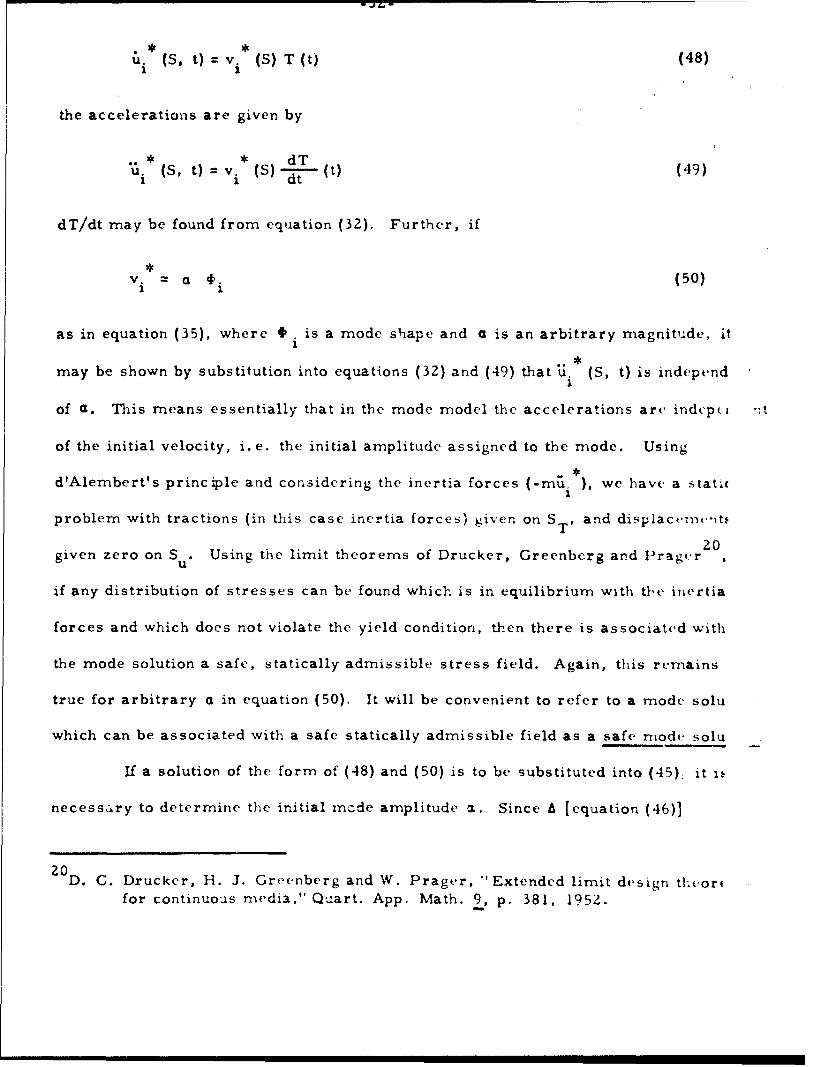
u. (S, t) =v. (S) T (t) (48)1 (STt

the accelerations are given by

** dTu. (S t) = v. (S)- (t) (49)

1 1 t

dT/dt may be found from equation (32). Further, if

v. a $. (50)1 1

as in equation (35), where 4 is a mode shape and a is an arbitrary magnitude, itI*

may be shown by substitution into equations (32) and (49) that U. (S, t) is independ1

of d. This means essentially that in the mode model the accelerations ar, ind-ptl t

of the initial velocity, i.e. the initial amplitude assigned to the mode. Using

d'Alembert's principle and considering the inertia forces (-ma i ), we have a stati(

problem with tractions (in this case inertia forces) given on ST, and displacome'• t,

2.0given zero on S . Using the limit theorems of Drucker, Greenberg and Prag,.rU

if any distribution of stresses can be found which is in equilibrium with the inertia

forces and which does not violate the yield condition, then there is associated with

the mode solution a safe, statically admissible stress field. Again, this remains

true for arbitrary a in equation (50). It will be convenient to refer to a mode solu

which can be associated with a safe statically admissible field as a safe mode solu

If a solution of the form of (48) and (50) is to be substituted into (45); it iý

necessary to determine the initial mcde amplitude a. Since A [equation (46)]

20D. C. Drucker, H. J. Greenberg and W. Prager, "Extended limit design theortfor continuous media," Quart. App. Math. 9, p. 381, 1952.

-33-

measu,'es the difference between the solutions, it is logical to choose a such that

A 0 is as small as possible. This may be written as

d jm (v -a I)(v. - at.)dS O0d a S 2 i i i

Differentiating and solvir.g for C., we obtain

m v. 4. dS

1 1S

m .A. dS

S

Comparison with equation (39) shows that the result is identical to that obtained

earlier by a different argument. Multiplying through by a, we see that, using (50).

ma . at, dS = my. v. dS mv.v. dSS S 1 1 S

or

m (v. -v. v, dS- 0S I

Equation (53a) may be used to show that, if (52) is satisfied,

0 v v. dS - v.Sv. dSS S

i.e. the initial measure of difference is simply the initial difference between the

energies of the solutions. Equation (53b) shows that the difference between v. and1

v. is orthogonal to v, ; this result is suggestive of elastic normal mode analysis,1 1

considering v. to be analogous to any one mode.1

This discussion indicates that the choice of a safe mode solution to

approximate the unknown solution leads to initial conditions identical to those found

earlier, and further to an assurance that a measure of the differences between the

solutions must decrease. If the initial difference is small, i.e. small compared

to the initial energy in any one solution, we are provided with a reliable check of

the validity of the one degree of freedom model. No arbitrary assumptions, other

than the choice of a mode shape, need be made.

One further useful piece of information may be added. From a proposition

due to Martin 2 1 , the time t at which the velocities &t vanish in the real solution1

can be written

mv.vv. dSI I

tf - 1dS (55)

S

where v. is the initial mode velocity and 1D is the initial rate of energy dissipation1

in the mode. (This proposition does not require that the mode be a safe mode.)

However, from (34), (32) and (53a),

21J. B. Martin, "Impulsive loading theorems for rigid plastic continua," Proc.

Eng. Mech. Div., A.S. C.E., 90 (EM5), p. 2 7, 1964.

rnv. v. dS mvivi dS

t f S . . .=. ..... (56)

D ds 6DdsS aS

provided that the initial amplitude of the mode satisfies the optimum requirement

that A0 be a minimum. Hence

tf >tf (57)

i.e. the velocities in the model vanish before the velocities in the actual solution.

Experience shows that tf and tf are very often equal, and in most cases the

difference is small.

In the following section we shall discuss the application of this method to

illustrative examples.

5. EXAMPLES

In order to demonstrate the effectiveness of the approximation using the mode

solution we shall compare the results of the solutions discussed in Y2 with their

approximations.

(i) Consider first the clamped beam shown in Figs. 6(a) and 9(a). The final

central displacement is given in equations (17) and (18), and is a function of b/I.

A. mode solution has been found for this problem, Fig. 9(c), and the final displacement

is given in equation (44). It remains to check that the mode chosen is indeed a safe

mode, and to find the relative value of the initial difference A6.

The acceleration of the central point in the beam in the mode solution may

be easily calculated from the initial central velocity [ equation (42)] and the time of

duration [ equaLion (43)] since it is known that the velocity-time relation is linear.

This is given by

24M

ml2

Using d'Alembert's principle, the loading diagram for the beam is shown in Fig. 11(a)

and the bending moment diagram is shown in Fig. 1 l(b). It is readily shown that the

maximum bending moment is M , and that it always occurs in the center of the beam.0

Hence the mode is a safe mode solution. In order to compute A we make use of

equation (54). A relative measure of the magnitude of e0 may be obtained by dividing

0 0a by the initial energy of the actual problem. Let this be K . Then

-37-

IK0 I mbV 2 (59a)

2 0

P 1 2m2.A =• mbv 2 2 uo2 dx

1 2 3 2 2b b)2 22 mbvo- m ov (59b)

Sj _.3 _.b b2= " -(2 _ b ) (59c)

0- 4 1 1

The final central displacement computations have been plotted in Fig. 12. In ad(

to the actual and mode solutions, the upper bound which may be computed by a m

proposed by Martin21 is given. In Fig. 13 the mode solution error and the ratio

A °/K° are plotted on the same figure. This diagram shows that the error is sm

when A°/K° is small, and that the error increases as A°/K° increases. It cai

be expected that the error is zero when A°/K° is a minimu-n, and indeed this ik

SO.

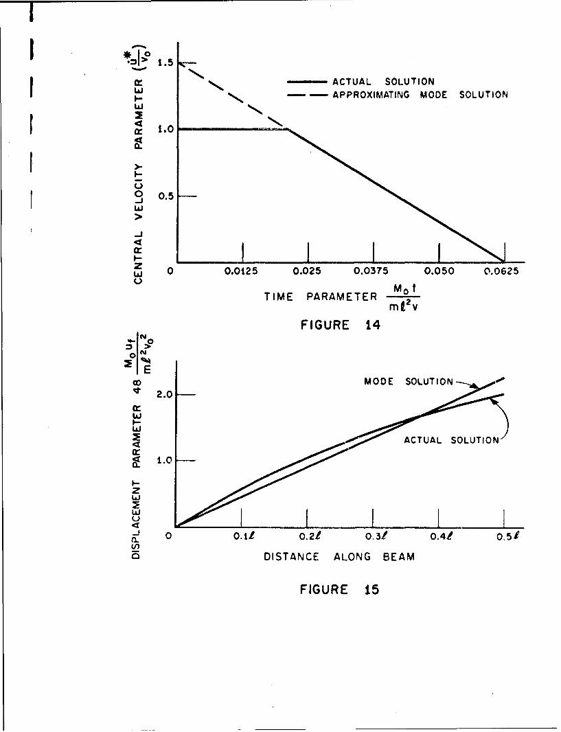
Figs. 14 and 15 give further details for the case of b/I = I. Fig. 14 gi

the central velocity-tir curves for the actual solution and the mode solution. It

be seen that the velocities coincide after one third of thc total deformation time h

elapsed. In fact the velocities coincide everywhere on the beam during this peric

and A [equation (46b)] is zero. Thls A decreases rapidly (and in this case

vanishes) even though A0/KO (Fig. 13) has an appreciable magnitude.

Fig. 15 compares the final shapes of the deformed beams for the case

b/I = 1, showing that the displacements in the mode solution overestimate the actual

displacements in some regions, and underestimate them in others.

A mode solution for the pinned end case of the beam discussed above

(Fig. 7a) may be obtained in a manner identical to that for the clamped case. The

mode shape is taken to be that in Fig. 9(c). The initial amplitude is not affected by

the change in boundary conditions, but the deformation time tf is simply doubled.

It may readily be shown that this is a safe mode solution. A comparison of the

approximate solution with the actual solution for the central displacement19 for

two values of b/1 is given in Fig. 16.

(ii) Consider secondly the cantilever with an attached tip mass shown in Fig. 4.

The solution, giving the tip mass velocity as a function of time, appears in equations

(8) and (10). The final tip mass dizplacement is given in equation (11).

In this case a good guess at a mode solution is clearly a velocity field

involving a rigid body rotation about the support, shown in Fig. 17. The velocity

field and rotation rate at the base may be written in terms of •*, the velocity of

the tip mass. From equations (28) and (32), the acceleration of the tip mass will be

, (M /i) - - - M (60)• . 1 o260

G (i ,)2 + m ( X2) 2 dx G1 (1

0

where y = mI/ZG as before. The bending moment diagram may now be drawn, and

is shown in Fig. 18. It may readily be seen that the bending moment does not exceed

M at any point for any value of y Hcnce the chosen approximation is a safe0

mode solution.

The optimum initial value of the tip velocity z may be found as befor

The actual initial velocity is zero except at the tip where it has value v. If v

is the initial value of z , we require, from equation (53a),

Gv v=G(v + m( 4. v)2 dx

*0

v 1v = 2 (61)I +=Y

The tip mass velocity is then given by

z ( t=- = ... . .. (• -- (62)v + --2 Y tf3 f

where, from equation (56)

t Gvz Gfvt = - -*

f 0* M

Fig. 19 shows the tip mass velocities plotted for the actual solution

[equations (8) and (10)] and for the mode solution, for the particular case y =.

In this case it is seen that the velocities are the same for M t/GIv >0. 167; it ma

readily be shown that A vanishes at time M t/GIv = 0. 167.0

-40-

The final tip displacement is a function of the parameter y , and hence the

accuracy of the approximation will depend on Y . The final tip displacements have

been plotted as a function of Y in Fig. 20, and show that the discrepancy varies

from zero at Y = 0 to an underestimate of about 15% at y = 3. On the same

figure A°/K° has been plotted. When Y = 3 AO/KO has the value 0. 67. Despite

this large value of A°/K° the approximation is fairly good.

One further example is summarized in Fig. 21. In this case the energy

ratio A°/K° is extremely small. Considering the areas under the curves to

obtain displacements at the center of the beams, it can be seen that the difference

between the actual solution and the mode solution is extremely small.

-41-

6. C O N C L US_ _ O NS_

In this paper an attempt has been made to rationalize the setting up of i

one degree of freedom approximation in elementary rigid-plastic theory for imp

loading. The method requires that a mode shape be chosen; thereafter. the

deceleration (or the equivalent spring force and mass) and the initial mode veloc

follow without further assumptions. The concept o0 a safe m.ode arid the analysi,

given in Section 4 provide a criterlotn by which good mode approximations may b

recognized. For illustrative purposes the meti-od has beet, applied to extremely

simple examples. There is no conceptual difficulty in applyirg the technique to I

more complicated cases.

It is seen that even in cases where P°K is fairly large the approximý

tion can be reasonably good. Only where sfiK° is smal', however, can it be

taken that the approximation will certainly be good. The ot;'er cases enphasize

that good approximations can be obtained whe:. •°'K is large, as ":.ndoubtedly

good approximatiorn could be obtdined with mode soL-tions wncl were not sate Ir.

the sense used iti this paper. This paper si.ows o-)Iy thait a certain limited c!ass

of mode approximations can be considered reliable.

The technlq.,e described could be applied with c'-anges, to probleois wit

time dependent loading and to certdi,, oti er viscous type mnaterial idealizatiols

such as rigid-visco-plastic. Attempts are being marde to develop ,.sef1ii approxi-

mating techniques for these cases.

ACKNOWLEDGEMENT

The results given in this paper were obtained in the course of research

sponsored by the Underwater Explosions Research Division, David Taylor Modei

Basin, under Contract N189(181)-57827 A(x).

I!

II QQO

QQi

II

FIGURE I FIGURE 2

!II V

I

I FIGURE 3

I

VELOCITY vAT TIME t=O

mas-s/unit length m MASS G

FIGURE 4

C A

VELOCITY DIAGRAM

(C)

Mo Mo Mo

Cf -1B B••' •• A

FREE BODY DIAGRAMS

(b)

FIGURE 5

1I

1~~ ~ u (I /4TTTIvo

I_ _A 6 C

I

I VELOCITY

( A C DIAGRAMS(b) vo tao0

A P B 0 C

I (C ) I v° 0 -< t -<5 HjsFIRST

PHASEI Zi Z

A P B C

t (d) v(t) tI -t -5t2

IA

SECOND(e) • v(t) t2 5 t t HASE

FIGURE 6

It

Kb

(a) AB c ---

000

A B C

(b) v,(t) vo

ZIz

A P B C

v, M t(C) v (t)

Mo

(d ) ( 0:6 1 - 1= = :( R, PLASTIC

REGION

FIGURE 7

xx

(a) (b)

FIGURE 8

bý4 iý ý iý Vo mass m per

,,,__ _ unit length

I)

L 10 ÷-(0)

(b)

(b)

FIGURE 9

~ SINECURVE

FIGURE 10

M ••24 M°

6M°A•

LOADING DIAGRAM

L/M K [[6x 8x:

SENDING MOMENT DIAGRAM

FIGURE It

8.01

7.0

2 \yo 5.0

L,,I-

06.

Z; 4.0

ww

-J , ACTUAL SOLUTION

< 3.0

U,

-------- UPPER BOUND AFTER

4 MARTIN 2 1

-z

zw

o 2.0 K-b---..m 1.0r

-.

0 0. 2 0.4 0.6 0. 8 '1.0

b/f•

FIGURE 12

1.0

0.75

z0.50 20 0

10-

-J0

0.25 10 .

0

0 0 00 0.00*

blf 0

-10w

MODE SOLUTION z

-20 w0.

FIGURE 13

I,-

0 0 .5w

TIM P A PR OXIMATIN MO D SO UTO

>0

2.0

-J

c-

4

zw 0 OOt.5 0.025 0.0375 0.050 0.0625

TIME PARAMETER BEAM

FIGURE 14q-NO

qJ 2.0

LJ oot o2o./o._o5.I.-L ITNC LNGBA

FIUE4

8.00

7.0

0 >

°2 6.0

w

"4 5.0

zX. 4.0

w

0.

3.0-J\

z MODE APPROXIMATIONwu 2.0 0

0 COMPUTED POINTS FOR,, CORRECT SOLUTIONz

1.0

0 0.2 0.4 0.6 0.8 1.0

b t6

FIGURE 16

Amr/unit lengthG

A B

T

FIGURE 17

B

FIGURE 18

1.0

0.8.NI >cr f ACTUAL SOLUTION

I-w

S0.64crN

)-

-J 0.40

>• APPROXIMATECL SOLUTION

•-- 0.2 -

0 0.2 0.4 0.6 0.8 1.0Mot

TIME PARAMETER motGiv

FIGURE 19 COMPARISON OF CORRECT AND APPROXIMATE

TIP VELOCITY-TIME CURVES FOR

IMPULSIVELY LOADED CANTILEVERWITH y i

zw

NoIamos 1'4fl1DV NI AS83N3 ON -W

MON1* NI A983N3-NQIufl1s -l1fl1V NI A0)83N3 o

0 -0

w

Zr /

a.. E~ CL.

<- 00

-JJ cin/ H 0

0r

U-/

30

00

0 ODNYC

zA! Z/ 0ROIN 313VYV8Vd IN3vY3:DV11dSIG d~li

w

'o00 0 of

w 202 0-cf

p. I- >.- wa

0In 0 ..jw 0 LL

COLE -

0 02c4 i cr - c

In LaJ wi-J WJ ozLa.J,4 2 LLCI)

4 4 4 j

- 2 z4r w 0J 07

C)n 4 0 IT

0 w

oc

0

0 Q.a.Q10a C

a.I.

4. crJ

40

0 000 &0

6 6;

8-3-1 ±31NV8Vd Lit:013A -1VUIN30

DISTRIBUTION LIST FOR UNCLASSIFIEDTECHNICAL REPORT ISSUED UNDER

CONTRACT N189(181)-57827A(X)

Serials

CH BUSHIPS

1-2 Code Z2OL3 341A4 423

* 5-6 CHONR7 COM, NOL (White Oak)

8-9 DIR, NRLI 10 CO & DIR, USNUSL

11-30 DIR, DDC

iII

i*

IIIIU

3 UNCLASSIFIED

DOCUIMNT CONTROL DATA - R&D,f tap' .JmL.edUmi of U410. 6 de 0i, and aills6 lalini nof be soft"m meo i *O-t now i•bept*~,

I. 0414WT0i ACT•TVY (c"IA 010" 1. RKPORT 89CUMITY C L-aGIVICATIO"Division of Engineering Unclas sified

•" Brown Universityllb. *"*up

I Providence, R. I.

"MODE APPROXIMATIONS FOR IMPULSIVELY LOADED RIGID PLASTICSTRUCTURES

4. o*afl"rv "Pt e r" of now w .=is.,lw. be)

S. AUT11f* 44as6 NOeR MNi .0me., W&aV '

- - Martin, J. B. and Symonds, P. S.

6. lopeNT •S.. 70. TOTAL NO. OF PAeUS 7 me.. Oe MoftMay 1965 57] 21

S41. CONTRACT ON GOAT? NO. OmeimATOnwai asPOrT osummus)

"N189(181)-578Z7A(X) (Dept. of Navy) BU/DTMB/6& PROJest Iro.

1t. AVAILAUSLITY/?ikTATIoUI OTIGCDistribution of this document is unlimited.

11. SUPPL 6MUTARY NVuOm It. SPON&sRG WLITARY ACTIVITY

David Taylor Model BasinDepartment of the Navy

13. ANSTRACT

An attempt is made to provide a rational method of constructing- - one degree of freedom approximations for impulsively loaded metal

structures which are analysed according to an elementary rigid-plastictheory. The approximation follows automatically from a chosen modeshape, and a criterion for determining good mode shapes is introduced.

DD 1473 UNCLASSIFIEDSecurity Clasaificatice

Security Classification _____

KYWRSROLF WT ROLF WI' ROLE9 "T

Loading (Mechanics) LN IKULN

Structures, rigid-plasticDeformnationDynamics, structuralMode approximationsTheoryI

INSTRUCTIONS

1. ORIGINATING ACTIVITY: Enter the name and address imposed by security classification. using standard statementotof the contractor, subcontractor, grant**. Department of Do- such as:fenae activity or other organixation (corporate author) issuing (1) "'Qualified requ.estesr may obtain copies of thisthe report. report from DDC."2&. REPORT SECUETY CLASSIFICATION: Enter the over- (2) "Foreign announcement and dissemination of thisall security classification of the repoi.t Indicate whitherreotb Cisntuhti"f"Restricted Vata" in Included. Iarking is to be In accord. eotb D sntatoie.ance with appropriate security regulations. (3) "U. S. Government agencies may obtain copies of

2b. ROU~ Atomtic ownadig I speifid i Do D~this report directly from DDC. Other qualified DDCrectlve 3200. 10 and Armed Forcae Industrial Maul Entsrsealreuetthogthe group numbr. Also, when applicable, show that optionalmarkings have been used for Group 3 and Group 4 -as author- (4) "U. S. military agencies may obtain copies of thisized. report directly from DDC. Other qualified users3. REPORT TITLE.- Enter the complete report title In all shall request throughcapital letters. Titles in all cases should be unclassified.If a meaningful title cannot be selected without classifica-tion. show, title classification In all capitals in parenthesis (5) "All distribution of this rsport is controlled. Qu~al-immediately following the title. ified DDC users &hall request through

4. DRSCRIPTIVE NOTES: If appropriate, enter the type of ________off_______

report eg.g, interim, progress, summary, annual, or final. If the report has boen furnished to the Office of To-..hnicalGive the inclusive date* when a specific reporting period is Services, Department of Commerce, for sale to the public. Indi-covered,. cat* this fact and enter the price, if known.S. AMHTIR(S) Enter the name(*) of author(s) as shown on IL. SUPPLEMENTARY NOTES:- Use for additloial oxplano-or in the report. Enter last name, first name. middle Initial, tory notes.It military, show rank and branch of service. The name ofJthe principal author is an absolute minimum requirement. 12. SPONSORING MILITARY ACTIVIY: Enter the name of

the departmental project office or laboratory sponsoring (pay-6. REVORT .1ATL_ Enter the date of the report as day. in for) the research and development. Include add&ea.month, year; or month, year. It more than one date appearson the report, use date of publication. 13. ABSTRACT: Enter an abstract giving a brief and factual

summary of the document indicative of the report. even though7.TOTAL. NUMBER OF PAGES: The total page count it may also appear elsewhere In the body of the technical re-

should follow normal paglnaL..nt procedures, Le., enter the port. If additional space is required. a continuation sheet shall,number of pages containing information, be attached.7b. NUMBER OF REFERENCES: Enter the total number of It in highly desirable that the abetract of classified reportsreferences cited in the report. be unclassified. Each paragraph of the abstract shall end withBe. CONTRACT OR GRANT NUMBER. If appropriate, enter an indication of the military security classification of the in.the applicable number of the contract or prant under which formation in the paragraph, represented as (7's). (s), (c),., at()the report was written. There is no Limitation on the length Of the abstract. How.9b, S. Ss 6d. PROJECT NUMBER: Enter the appropriate ever, the suggested 'ength is from 150 to 223 words.military department identification, such as project number, 1.KYWOD: aywrsrethnclymnifutrmsubproject number, system numbers, task number, etc.14KEWOD:eywrso*tcnalymnigutrs

or short phrases that characterize a report and may be used as9a. ORIGINATO>R'S REPORT NUMBER(S): Entter the f in- index entries for cataloging the report. Xey words must becisi report number by which the document will be identified selected so that no security clsssiflcstion Is required. ldentl-and controlled by the originating activity. This number must flora, such as equipment model desigration, trade name, militarybe unique to this report. project code name, geographic location, may be used as key9b. OTHER REPORT NUMBERS): If the report haa been words but will be followed by an indication of technical con-

ssslignod any other report numbers (either by the originator text. The assignment of links, risles, end weights in optional.or by~ the eponsor). also enter this number(s).

10. AVAU..ABILITY/L.IMITATION NOTICE&: Enter any Unit-itations on further dissemination of the report. other than thosel

DD 2AJ A0 * 1413 (BACK) U-IN.C I-ASS IFIE DSecurity Classification