quick test for percent of deleterious material -...

Organizational Results Research Report August 2009 OR10.005

Quick Test for Percent of Deleterious Material

Prepared by Missouri University of

Science and Technology and

Missouri Department of

Transportation

TECHNICAL REPORT DOCUMENTATION PAGE.

1. Report No.: 2. Government Accession No.: 3. Recipient's Catalog No.: 4. Title and Subtitle: 5. Report Date: Quick Test for Percent of Deleterious Material

August 28, 2009 6. Performing Organization Code:

7. Author(s): David N. Richardson 8. Performing Organization Report No.: RI07-052

9. Performing Organization Name and Address: 10. Work Unit No.: Missouri University of Science and Technology 1870 Miner Circle

11. Contract or Grant No.:

Rolla, MO 65409 12. Sponsoring Agency Name and Address: 13. Type of Report and Period

Covered: Missouri Department of Transportation Organizational Results PO Box 270, Jefferson City, MO 65102

Final Report. 14. Sponsoring Agency Code:

15. Supplementary Notes: The investigation was conducted in cooperation with the U. S. Department of Transportation, Federal Highway Administration. 16. Abstract: The Missouri Department of Transportation (MoDOT) is considering the replacement of its deleterious materials test method (TM-71) with test methods that are more objective. MoDOT contracted with the Missouri University of Science and Technology (Missouri S&T) to develop a system of test methods. Nine quarry/ledge samples representing seven geologic formations (four limestones and three dolomites) were supplied by MoDOT. The ledge samples represented three aggregates each for use in concrete, asphalt, and granular base. Samples with controlled contamination were also tested, bringing the total to 18. The aggregates were subjected to fifteen test methods. This data, coupled with MoDOT historical specific gravity, absorption, and TM-71 deleterious materials data of the samples formed the basis of the test study dataset. Multiple linear regression was used to produce 15 models of varying accuracy and complexity for TM-71 predictions. The TM-71 deleterious data were used as the response (dependent) variables. The best models entailed test methods not normally performed by MoDOT, such as sieved slake durability, point load strength, vacuum saturated bulk specific gravity/absorption, and aggregate crushing value, along with the more. familiar micro-Deval and plasticity index. Model adjusted-R2 values ranged from 0.603 to 0.895. Thus, three to four options (models) were open to MoDOT for consideration for each type of deleterious material (Total Deleterious Material, Total Deleterious Material Plus Hard Chert, Deleterious Rock Plus Soft Chert, and Shale). As an alternate to the regression models, a threshold-limits method was presented. The models themselves were not exact enough to predict the various deleterious contents with the level of accuracy required for routine decisions concerning aggregate product acceptance or rejection. As a result, a method of baseline ledge-specific initial calibration of the models was developed to enable MoDOT inspectors to make acceptability decisions on a routine basis without the necessity of performing TM-71. 17. Key Words: 18. Distribution Statement: deleterious material; aggregate No restrictions. This document is available to

the public through National Technical Information Center, Springfield, Virginia 22161.

19. Security Classification (of this 20. Security Classification (of this 21. No of Pages: 22. Price: report): page): Unclassified. Unclassified. 166

Form DOT F 1700.7 (06/98).

FINAL REPORT RI07-052

QUICK TEST for PERCENT OF DELETERIOUS MATERIAL

Prepared for the

Missouri Department of Transportation Organizational Results

By

David N. Richardson, PE

Missouri University of Science and Technology

August 28, 2009

The opinions, findings, and conclusions expressed in this report are those of the principal investigator and the Missouri Department of Transportation. They are not necessarily those of the U.S. Department of Transportation or the Federal Highway Administration. This report does not constitute a standard, specification, or regulation.

ii

ACKNOWLEDGEMENTS

The author wishes to thank the Missouri Department of Transportation (MoDOT) for sponsoring this work and Paul Hilchen, Will Stalcup, and Jennifer Harper for their coordination and support. On the Missouri University of Science and Technology (Missouri S&T) side, thanks go to Gary Davis, Karl Beckemeier, and Michael Keaton for their many hours in the laboratory, and to Michael Lusher for his contributions both in the laboratory and with statistical computation assistance.

iii

EXECUTIVE SUMMARY

The Missouri Department of Transportation (MoDOT) is considering the replacement of its deleterious materials test method (TM-71) with test methods that are more objective. MoDOT contracted with the Missouri University of Science and Technology (Missouri S&T) to develop a method of approximation of various deleterious materials contents based primarily on systems of standard tests which would augment or replace the deleterious test method TM-71. The system would be comprised of one or more objective tests, depending on the outcome of the research project. Nine different quarry/ledge production materials representing seven geologic formations (four limestones and three dolomites) were sampled by MoDOT and delivered to Missouri S&T. The samples represented three aggregates each for use in concrete, asphalt, and granular base. Samples of controlled contamination were also tested, bringing the total to 18. The aggregates were subjected to fifteen different test methods/method modifications. The test results, coupled with MoDOT historical specific gravity, absorption, and deleterious materials data, formed the basis of the study dataset. The test methods were: Los Angeles abrasion, micro-Deval, wet ball mill, wet ball mill-modified, aggregate crushing value, methylene blue value, sodium sulfate soundness, water-alcohol freeze-thaw soundness, point load strength (dry and wet), vacuum saturated bulk specific gravity, vacuum saturated absorption, sand equivalent, plasticity index, and sieved slake durability. Results from historical MoDOT test methods included gradation, bulk specific gravity, absorption, deleterious rock content, shale content, and chert content. Multiple linear regression was used to produce 15 models of varying accuracy and complexity for TM-71 predictions. Deleterious data for the same aggregate materials (samples) were used as the response (dependent) variable. The best models entailed test methods not normally performed by MoDOT, such as sieved slake durability, point load strength, vacuum saturated bulk specific gravity/absorption, and aggregate crushing value, along with the more familiar micro-Deval and plasticity index. Model adjusted-R2 values ranged from 0.603 to 0.895. Thus, three to four options (models) were open to MoDOT for consideration for each type of deleterious material (Total Deleterious Material, Total Deleterious Material Plus Hard Chert, Deleterious Rock Plus Soft Chert, and Shale). As an alternate to the regression models, a threshold-limits method was presented. The models themselves were not exact enough to predict the various deleterious contents with the level of accuracy required for routine decisions concerning aggregate product acceptance or rejection. As a result, a method of baseline ledge-specific initial calibration of the models was developed to enable MoDOT inspectors to make acceptability decisions on a routine basis without the necessity of performing TM-71.

iv

Unfortunately, MoDOT had no historical data with which to verify the models. This is a vital step and must be done in the future before any of the models are implemented.

v

TABLE OF CONTENTS

ACKNOWLEDGEMENTS .......................................................................................... II

EXECUTIVE SUMMARY .......................................................................................... III

TABLE OF CONTENTS.............................................................................................V

LIST OF FIGURES ...................................................................................................XI

LIST OF TABLES.................................................................................................... XV

INTRODUCTION ....................................................................................................... 1

GENERAL .............................................................................................................. 1

RESEARCH PROJECT AGGREGATE TESTING.................................................. 6

MoDOT CONTRIBUTION ...................................................................................... 6

POTENTIAL PROBLEMS ...................................................................................... 6

OBJECTIVE............................................................................................................... 7

LITERATURE REVIEW ............................................................................................. 8

DELETERIOUS MATERIALS................................................................................. 8

DELINEATION OF DELETERIOUS MATERIALS.................................................. 8

DELETERIOUS ACTIONS ..................................................................................... 9

Impact and Abrasion Action ................................................................................ 9

Los Angeles Abrasion ..................................................................................... 9 Micro-Deval ................................................................................................... 10 Wet Ball Mill .................................................................................................. 11 Sieved Slake Durability ................................................................................. 11

Crushing/Cracking During Loading Action ........................................................ 11

Aggregate Crushing Value ............................................................................ 12 Point Load Strength ...................................................................................... 12

Swelling/Shrinkage and Breakdown from Wetting/Drying................................. 13

Delta Point Load Strength ............................................................................. 13 Freeze/Thaw Action.......................................................................................... 13

Pore Characteristics ...................................................................................... 14 Absorption ................................................................................................. 14 Bulk Specific Gravity.................................................................................. 15 Vacuum Saturated Absorption................................................................... 15

vi

Vacuum Saturated Specific Gravity ........................................................... 16 Water-Alcohol Freeze-Thaw and Sulfate Soundness ................................ 16

Elastic Accommodation/Strength .................................................................. 16 Aggregate Crushing Value and Point Load Strength ................................. 17 Los Angeles Abrasion................................................................................ 17 Micro-Deval ............................................................................................... 17 Water-Alcohol Freeze-Thaw Soundness ................................................... 17 Magnesium and Sodium Sulfate Soundness ............................................. 18 Wet Ball Mill ............................................................................................... 19

Mineralogy..................................................................................................... 19 Asphalt-Aggregate Bond Interference............................................................... 19

Plasticity Index .............................................................................................. 20 Sand Equivalent ............................................................................................ 21 Methylene Blue ............................................................................................. 22

Cement-Aggregate Bond Interference .............................................................. 22

Water Absorption by Highly Plastic Fines ......................................................... 23

Clay Lubrication ................................................................................................ 23

SYSTEM ESTIMATION OF AGGREGATE DELETERIOUS MATERIAL

CONTENT............................................................................................................ 23

SUMMARY........................................................................................................... 24

TECHNICAL APPROACH ....................................................................................... 26

GENERAL ............................................................................................................ 26

Experimental Design......................................................................................... 26

Replicate Specimens ........................................................................................ 26

MATERIALS......................................................................................................... 26

MoDOT DATA ...................................................................................................... 28

DELETERIOUS MATERIAL SEEDED SAMPLES................................................ 29

Type and Origin of Seed Material ..................................................................... 30

Amount of Seed Material .................................................................................. 32

TEST PROCEDURES and EQUIPMENT............................................................. 35

Seeding ............................................................................................................ 35

Impact Breakage and Abrasion......................................................................... 36

Los Angeles Abrasion ................................................................................... 36 Micro-Deval ................................................................................................... 36 Wet Ball Mill .................................................................................................. 36 Sieved Slake Durability ................................................................................. 37

vii

Crushing Under Loading................................................................................... 38

Aggregate Crushing Value ............................................................................ 38 Point Load Strength ...................................................................................... 39

Breakdown from Wetting/Drying (Swelling/Shrinking)....................................... 41

Sieved Slake Durability ................................................................................. 41 Wet Ball Mill .................................................................................................. 41 Micro-Deval ................................................................................................... 41 Delta Point Load Strength ............................................................................. 41 Plasticity Index .............................................................................................. 41 Methylene Blue ............................................................................................. 42 Sand Equivalent ............................................................................................ 42

Expansion/Contraction from Freezing/Thawing ................................................ 42

Aggregate Pore Characteristics .................................................................... 42 Absorption and Bulk Specific Gravity......................................................... 42 Vacuum Saturated Absorption and Bulk Specific Gravity .......................... 43 Water-Alcohol Freeze Thaw ...................................................................... 44 Sodium Sulfate Soundness ....................................................................... 44

Pore Length................................................................................................... 44 Mineralogy..................................................................................................... 45

Methylene Blue, Plasticity Index, and Sand Equivalent ............................. 45 Water-Alcohol Freeze-Thaw ...................................................................... 45

Elastic Accomodation/Strength ..................................................................... 45 Aggregate Crushing Value, Los Angeles Abrasion, Micro-Deval, Point Load Strength, Wet Ball Mill ............................................................................... 45 Water-Alcohol Freeze-Thaw ...................................................................... 45

Asphalt Binder Bond Interference ..................................................................... 45

Methylene Blue, Plasticity Index, and Sand Equivalent................................. 45 Water Absorption .............................................................................................. 45

Methylene Blue, Plasticity Index, and Sand Equivalent................................. 45 Concrete Paste Bond Interference.................................................................... 46

Methylene Blue, Plasticity Index, and Sand Equivalent................................. 46 Clay Lubrication ................................................................................................ 46

Methylene Blue, Plasticity Index, and Sand Equivalent................................. 46

RESULTS AND DISCUSSION ................................................................................ 47

PRECISION AND OUTLIER ANALYSIS .............................................................. 47

TEST RESULTS................................................................................................... 48

Deleterious Materials Testing ........................................................................... 48

Aggregate Testing ............................................................................................ 48

CORRELATION ................................................................................................... 50

viii

Interrelated Test Correlations ........................................................................... 50

Impact Breakage and Abrasion ..................................................................... 51 Los Angeles Abrasion................................................................................ 51 Wet Ball Mill ............................................................................................... 53 Wet Ball Mill-Modified (WBMM) ................................................................. 53 Micro-Deval ............................................................................................... 57 Sieved Slake Durability.............................................................................. 57

Crushing Under Loading ............................................................................... 58 Aggregate Crushing Value......................................................................... 58 Point Load Strength................................................................................... 61

Swelling/Shrinkage and Breakdown from Wetting/Drying ............................. 62 Expansion/Contraction from Freezing/Thawing............................................. 62

Aggregate Pore Characteristics................................................................. 63 Absorption (T 85). ................................................................................. 63 Bulk Specific Gravity (T 85). .................................................................. 63 Vacuum Saturated Absorption. ............................................................. 64 Vacuum Saturated Bulk Specific Gravity. .............................................. 64 Sodium Sulfate Soundness.................................................................... 69

Mineralogy ................................................................................................. 70 Methylene Blue. ..................................................................................... 70 Sand Equivalent. .................................................................................... 71 Plasticity Index. ..................................................................................... 71

Elastic Accommodation/Strength............................................................... 71 WAFT..................................................................................................... 72

Ranked Interrelated Correlation Coefficients .................................................... 72

Correlation with MoDOT Results ...................................................................... 73

Significance of Seeding .................................................................................... 75

Correlation of Deleterious Materials with Individual Test Results ..................... 76

Deleterious Rock Soft Chert.......................................................................... 78 Shale ............................................................................................................. 81 Total Deleterious Materials............................................................................ 82 Total Deleterious Materials Hard Chert ......................................................... 85

REGRESSION ANALYSIS................................................................................... 88

Methodology ..................................................................................................... 88

Model Acceptance Criteria................................................................................ 89

R2 .................................................................................................................. 89 Adjusted R2 ................................................................................................... 89 Significance of Model .................................................................................... 89 Term Significance ......................................................................................... 89 Multi-Collinearity............................................................................................ 89 Undue Influence of Single Data Points.......................................................... 90 Normality of Test Residuals .......................................................................... 90

ix

Constant Variance of Residuals .................................................................... 90 Regression Models ........................................................................................... 90

T 85 Data ...................................................................................................... 91 TDM: Highest Adjusted R2 Four-Test Method Models................................... 91 TDM: Highest Adjusted R2 Three-Test Method Model .................................. 94 TDM: Two-Test Method Model...................................................................... 94 TDMHC: Highest Adjusted R2 Four-Test Method Models ............................. 95 TDMHC: Highest Adjusted R2 Three-Test Method Models ........................... 96 DRSC: Highest Adjusted R2 Four-Test Method Models ................................ 97 DRSC: Highest Adjusted R2 Three-Test Method Model ................................ 99 DRSC: Two-Test Method Model ................................................................... 99 Shale: Highest Adjusted R2 Three-Test Method Models ............................. 100

Estimation of Hard Chert ................................................................................ 103

Estimation of TDM .......................................................................................... 103

Estimation of TDMHC ..................................................................................... 103

Estimation of Soft Chert .................................................................................. 104

Summary ........................................................................................................ 104

VERIFICATION OF MODELS ............................................................................ 105

IMPLEMENTATION OF TEST METHODS ............................................................ 107

FLOWCHART ACCEPTANCE ........................................................................... 111

Threshold Limit Development ......................................................................... 111

CONCLUSIONS..................................................................................................... 116

TOTAL DELETERIOUS MATERIALS (TDM) MODELS ..................................... 116

TOTAL DELETERIOUS MATERIALS HARD CHERT (TDMHC) MODELS ....... 116

HARD CHERT.................................................................................................... 117

DELETERIOUS ROCK SOFT CHERT (DRSC) MODELS ................................. 117

SHALE MODELS ............................................................................................... 117

TEST METHODS ............................................................................................... 117

MODEL STRATEGIES....................................................................................... 118

THRESHOLD LIMITS......................................................................................... 119

RECOMMENDATIONS – FUTURE RESEARCH .................................................. 120

GLOSSARY ........................................................................................................... 121

REFERENCES ...................................................................................................... 122

x

APPENDICES........................................................................................................ 133

xi

LIST OF FIGURES

Figure 1: Shale Seed Material Hardness ................................................................. 31

Figure 2: Deleterious Rock Seed Material Hardness ............................................... 31

Figure 3: Distribution of Deleterious Rock Soft Chert in Samples ............................ 33

Figure 4: Distribution of Shale in Samples ............................................................... 33

Figure 5: Distribution of Hard Chert in Samples....................................................... 34

Figure 6: Distribution of Total Deleterious Material in Samples ............................... 34

Figure 7: Distribution of Total Deleterious Material Hard Chert in Samples ............. 35

Figure 8: Wet Ball Mill Device .................................................................................. 37

Figure 9: Sieved Slake Durability Device ................................................................. 38

Figure 10: Missouri S&T ACV Mold, Rod, and Plunger............................................ 39

Figure 11: Point Load Device................................................................................... 40

Figure 12: Vacuum Saturation Workstation ............................................................. 43

Figure 13: Wet Ball Mill vs. Los Angeles Abrasion................................................... 51

Figure 14: Wet Ball Mill Modified vs. Los Angeles Abrasion .................................... 52

Figure 15: Micro-Deval vs. Los Angeles Abrasion ................................................... 52

Figure 16: Los Angeles Abrasion vs. Point Load Strengthwet ................................... 53

Figure 17: Micro-Deval vs. Wet Ball Mill .................................................................. 54

Figure 18: Wet Ball Mill vs. Point Load Strengthwet .................................................. 54

Figure 19: Wet Ball Mill vs. Point Load Strengthdry................................................... 55

Figure 20: Wet Ball Mill vs. Wet Ball Mill-Modified ................................................... 55

Figure 21: Micro-Deval vs. Wet Ball Mill-Modified.................................................... 56

Figure 22: Wet Ball Mill-Modified vs. Point Load Strengthwet.................................... 56

Figure 23: Wet Ball Mill-Modified vs. Point Load Strengthdry .................................... 57

Figure 24: Micro-Deval vs. Point Load Strengthwet................................................... 58

Figure 25: Los Angeles Abrasion vs. Aggregate Crushing Value ............................ 59

Figure 26: Wet Ball Mill vs. Aggregate Crushing Value............................................ 59

Figure 27: Wet Ball Mill-Modified vs. Aggregate Crushing Value ............................. 60

Figure 28: Micro-Deval vs. Aggregate Crushing Value ............................................ 60

Figure 29: Aggregate Crushing Value vs. Point Load Strengthwet ............................ 61

xii

Figure 30: Aggregate Crushing Value vs. Point Load Strengthdry ............................ 61

Figure 31: Point Load Strengthwet vs. Point Load Strengthdry ................................... 62

Figure 32: Absorption vs. Bulk Specific Gravity (Dry) .............................................. 63

Figure 33: Bulk Specific Gravity (Dry) vs. Micro-Deval ............................................ 64

Figure 34: T 85 Absorption vs. Vacuum Saturated Absorption ................................ 65

Figure 35: Vacuum Saturated Absorption vs. Vacuum Saturated Bulk Specific

Gravity (Dry) ...................................................................................................... 65

Figure 36: Vacuum Saturated Bulk Specific Gravity vs. Absorption......................... 66

Figure 37: Vacuum Saturated Bulk Specific Gravity (Dry) vs. T 85 Bulk Specific

Gravity (Dry) ...................................................................................................... 67

Figure 38: Vacuum Saturated Bulk Specific Gravity (Dry) vs. Micro-Deval.............. 67

Figure 39: Vacuum Saturated Bulk Specific Gravity (Dry) vs. Los Angeles Abrasion

........................................................................................................................... 68

Figure 40: Vacuum Saturated Bulk Specific Gravity (Dry) vs. Wet Ball Mill ............. 68

Figure 41: Vacuum Saturated Bulk Specific Gravity (Dry) vs. Wet Ball Mill-Modified

........................................................................................................................... 69

Figure 42: T 85 Bulk Specific Gravity vs. Sodium Sulfate Soundness ..................... 69

Figure 43: Methylene Blue of Shale vs. Change in Sieved Slake Durability ............ 70

Figure 44: Methylene Blue vs. Vacuum Saturated Absorption ................................. 71

Figure 45: Delta Point Load Strength vs. Point Load Strengthdry ............................. 72

Figure 46: Comparison of MoDOT vs. Missouri S&T LAA Results........................... 74

Figure 47: Comparison of MoDOT vs. Missouri S&T NaSO4 Results ...................... 75

Figure 48: Comparison of MoDOT vs. Missouri S&T WAFT Results ....................... 75

Figure 49: Micro-Deval vs. Deleterious Rock Soft Chert Content ............................ 78

Figure 50: Wet Ball Mill-Modified vs. Deleterious Rock Soft Chert Content ............. 79

Figure 51: Wet Ball Mill vs. Deleterious Rock Soft Chert Content............................ 79

Figure 52: Los Angeles Abrasion vs. Deleterious Rock Soft Chert Content............. 80

Figure 53: Vacuum Saturated Bulk Specific Gravity vs. Deleterious Rock Soft Chert

Content .............................................................................................................. 80

Figure 54: Sieved Slake Durability vs. Deleterious Rock Soft Chert Content........... 81

Figure 55: Sieved Slake Durability vs. Shale Content.............................................. 82

xiii

Figure 56: Sieved Slake Durability vs. Total Deleterious Materials Content ............ 83

Figure 57: Micro-Deval vs. Total Deleterious Materials Content .............................. 83

Figure 58: Wet Ball Mill-Modified vs. Total Deleterious Materials Content ............... 84

Figure 59: Wet Ball Mill vs. Total Deleterious Materials Content ............................. 84

Figure 60: Los Angeles Abrasion vs. Total Deleterious Materials Content .............. 85

Figure 61: Sieved Slake Durability vs. Total Deleterious Material Hard Chert Content

........................................................................................................................... 86

Figure 62: Absorption vs. Total Deleterious Material Hard Chert Content ............... 86

Figure 63: Bulk Specific Gravity vs. Total Deleterious Material Hard Chert Content 87

Figure 64: Micro-Deval vs. Total Deleterious Material Hard Chert Content ............. 87

Figure 65: Vacuum Saturated Absorption vs. Total Deleterious Material Hard Chert

Content .............................................................................................................. 88

Figure 66: Measured vs. Predicted Total Deleterious Material: Four-Test Method

Model (1-a) ........................................................................................................ 93

Figure 67: Measured vs. Predicted Total Deleterious Material: Four-Test Method

Model (1-b) ........................................................................................................ 93

Figure 68: Measured vs. Predicted Total Deleterious Material: Three-Test Method

Model (1-c)......................................................................................................... 94

Figure 69: Measured vs. Predicted Total Deleterious Material Hard Chert: Four-Test

Method Model (2-a)............................................................................................ 95

Figure 70: Measured vs. Predicted Total Deleterious Material Hard Chert: Four-Test

Method Model (2-b)............................................................................................ 96

Figure 71: Measured vs. Predicted Total Deleterious Material Hard Chert: Three-

Test Method Model (2-c) .................................................................................... 97

Figure 72: Measured vs. Predicted Deleterious Rock Soft Chert: Four-Test Method

Model (3-a) ........................................................................................................ 98

Figure 73: Measured vs. Predicted Deleterious Rock Soft Chert: Four-Test Method

Model (3-b) ........................................................................................................ 99

Figure 74: Measured vs. Predicted Deleterious Rock Soft Chert: Three-Test Method

Model (3-c)....................................................................................................... 100

Figure 75: Measured vs. Predicted Shale: Three-Test Method Model (4-a) .......... 101

xiv

Figure 76: Measured vs. Predicted Shale: Four Test-Method Model (4b).............. 102

Figure 77: Measured vs. Predicted Shale: Three-Test Method Model (4-c)........... 103

Figure 78: Global Micro-Deval vs. Deleterious Rock Soft Chert ............................ 105

Figure 79: Global Micro-Deval vs. Total Deleterious Material ................................ 106

Figure 80: Slopes of TDMF vs. TDM Values.......................................................... 107

Figure 81: Method of TDMF Correction ................................................................. 109

Figure 82: Estimation of Slope “m” by PLSwet ........................................................ 110

Figure 83: Micro-Deval Threshold Limits ............................................................... 113

Figure 84: Los Angeles Abrasion Threshold Limits................................................ 113

Figure 85: Wet Ball Mill Threshold Limits ............................................................... 114

Figure 86: Sieved Slake Durability Threshold Limits.............................................. 114

Figure 87: Point Load Strengthdry Threshold Limits................................................ 115

xv

LIST OF TABLES

Table 1: Deleterious Material Types and Section 1000 Specifications for Coarse

Aggregate ............................................................................................................ 2

Table 2: Material Performance Problems, Causes, Relationships to Deleterious

Materials, and Test Methods................................................................................ 3

Table 3: Aggregate Materials................................................................................... 27

Table 4: Section 1007 As-Delivered Gradation Percent Passing............................. 28



Table 7: Percent of Deleterious Materials in Study Aggregates............................... 29

Table 8: Deleterious Material Used As Seed Material.............................................. 32

Table 9: Precision of Unseeded Test Methods ........................................................ 47

Table 10: Aggregate Test Result Averages ............................................................. 49

Table 11: Aggregate Test Result Averages, continued............................................ 49



Table 14: Interrelated Correlation Coefficients......................................................... 73

Table 15: Ranked Seeding Significance .................................................................. 76

Table 16: Correlation of Deleterious Rock-Plus-Soft Chert with Test Methods........ 77

Table 17: Correlation of Shale with Test Methods ................................................... 77

Table 18: Correlation of Total Deleterious Materials with Test Methods .................. 77

Table 19: Correlation of Total Deleterious Materials-Plus-Hard Chert with Test

Methods ............................................................................................................. 77

Table 20: Statistical Summary: Model 1-a ............................................................... 92

Table 21: Models of Each Deleterious Material in Order of Adjusted R2................ 104

Table 22: Example Threshold Limits for TDM........................................................ 112

1

INTRODUCTION

GENERAL The Missouri Department of Transportation (MoDOT) is considering the replacement of its deleterious materials test method (TM-71) with test methods that are more objective. MoDOT contracted with the Missouri University of Science and Technology (Missouri S&T) to develop a method of approximation of various deleterious materials contents based primarily on systems of standard tests which would augment or replace the deleterious test method TM-71. TM-71 is highly subjective in nature. It was envisioned that the system would take one of several forms, including a predictive regression equation(s) or a system of threshold limits. The system could be comprised of several tests, or a single test depending on the outcome of the research program. It was desired that the tests would easily simulate and quantify the specific deleterious actions of aggregates. The value of such a system of tests would be to progress toward a more objective method. Additionally, the certification of out-of-state testing personnel would become easier if MoDOT was using nationally-accepted standard tests rather than its own test method.

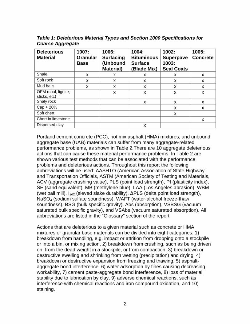
MoDOT specifications (MoDOT, 2004) distinguish between different forms of deleterious materials and assign levels of concern as to the deleterious materials’ presence in various aggregate products in two ways: 1) percent maximum allowable limits in materials specifications, and 2) by inclusion or absence in various material specifications in regard to usage. Table 1 shows the various deleterious types and the MoDOT specifications that include maximum limits in order of apparent concern and frequency. The table shows five different uses of aggregate, such as granular base. Some uses are not sensitive to certain deleterious materials, thus not all deleterious materials are limited by all aggregate specifications. Aggregate specifications limit deleterious materials by maximum allowable percent by weight. Table 1 shows nine specific types of deleterious materials as defined by TM-71. An “x” denotes that the specification limits the particular deleterious material. Deleterious material can be either inherent to the parent aggregate material or come from contamination, both natural or artificially generated. Typically, “other foreign material” (OFM) and “mud balls” would be included in the contamination category. All other deleterious materials types are intrinsic to the parent aggregate.

2

Table 1: Deleterious Material Types and Section 1000 Specifications for Coarse Aggregate

Deleterious 1007: 1006: 1004: 1002: 1005: Material Granular

Base Surfacing (Unbound Material)

Bituminous Surface (Blade Mix)

Superpave 1003: Seal Coats

Concrete

Shale x x x x x Soft rock x x x x x Mud balls x x x x x OFM (coal, lignite, sticks, etc)

x x x x

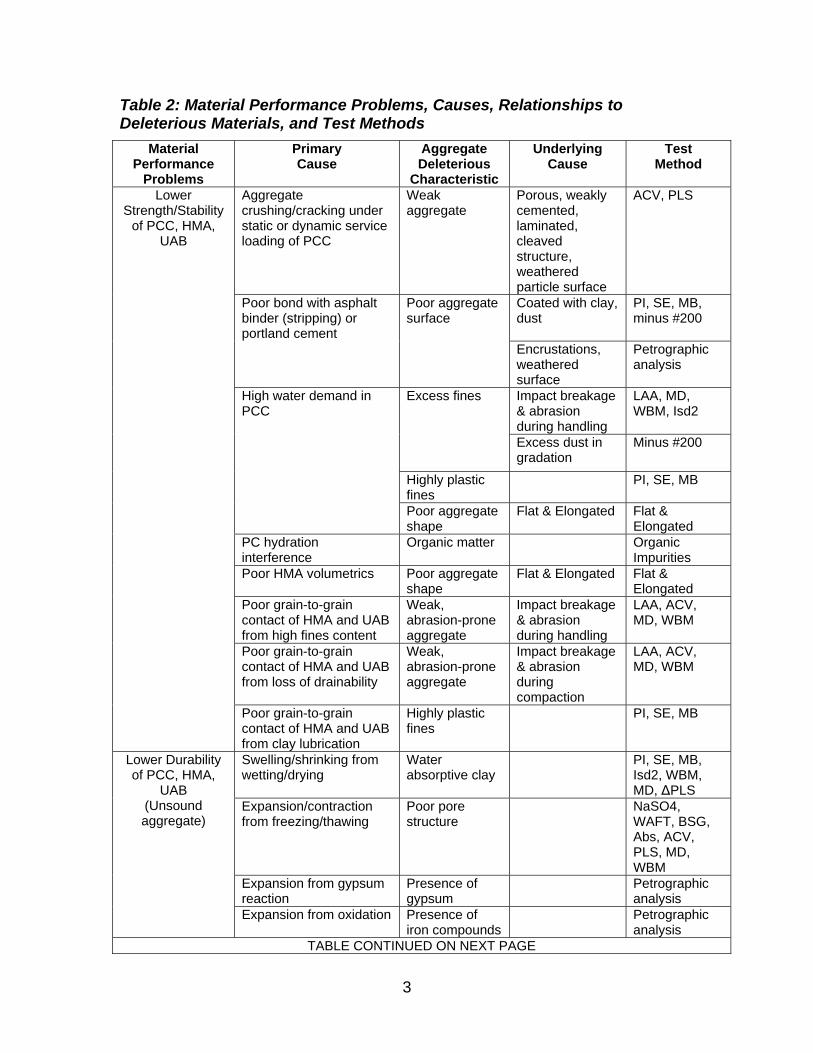
Shaly rock x x x Cap + 20% x x Soft chert x Chert in limestone x Dispersed clay x Portland cement concrete (PCC), hot mix asphalt (HMA) mixtures, and unbound aggregate base (UAB) materials can suffer from many aggregate-related performance problems, as shown in Table 2.There are 10 aggregate deleterious actions that can cause these material performance problems. In Table 2 are shown various test methods that can be associated with the performance problems and deleterious actions. Throughout this report the following abbreviations will be used: AASHTO (American Association of State Highway and Transportation Officials, ASTM (American Society of Testing and Materials, ACV (aggregate crushing value), PLS (point load strength), PI (plasticity index), SE (sand equivalent), MB (methylene blue), LAA (Los Angeles abrasion), WBM (wet ball mill), Isd2 (sieved slake durability), ΔPLS (delta point load strength), NaSO4 (sodium sulfate soundness), WAFT (water-alcohol freeze-thaw soundness), BSG (bulk specific gravity), Abs (absorption), VSBSG (vacuum saturated bulk specific gravity), and VSAbs (vacuum saturated absorption). All abbreviations are listed in the “Glossary” section of the report. Actions that are deleterious to a given material such as concrete or HMA mixtures or granular base materials can be divided into eight categories: 1) breakdown from handling, e.g. impact or attrition from dropping onto a stockpile or into a bin, or mixing action, 2) breakdown from crushing, such as being driven on, from the dead weight in a stockpile, or from compaction, 3) breakdown or destructive swelling and shrinking from wetting (precipitation) and drying, 4) breakdown or destructive expansion from freezing and thawing, 5) asphalt-aggregate bond interference, 6) water adsorption by fines causing decreasing workability, 7) cement paste-aggregate bond interference, 8) loss of material stability due to lubrication by clay, 9) adverse chemical reactions, such as interference with chemical reactions and iron compound oxidation, and 10) staining.

3

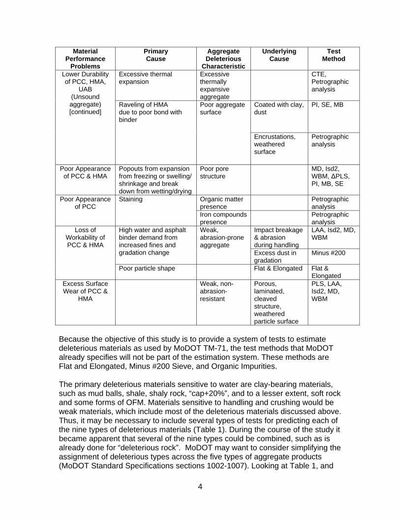
Table 2: Material Performance Problems, Causes, Relationships to Deleterious Materials, and Test Methods

Material Performance

Primary Cause

Aggregate Deleterious

Underlying Cause

Test Method

Problems Characteristic Lower Aggregate Weak Porous, weakly ACV, PLS

Strength/Stability crushing/cracking under aggregate cemented, of PCC, HMA, static or dynamic service laminated,

UAB loading of PCC cleaved structure, weathered particle surface

Poor bond with asphalt Poor aggregate Coated with clay, PI, SE, MB, binder (stripping) or surface dust minus #200 portland cement

Encrustations, Petrographic weathered analysis surface

High water demand in Excess fines Impact breakage LAA, MD, PCC & abrasion WBM, Isd2

during handling Excess dust in Minus #200 gradation

Highly plastic fines

PI, SE, MB

Poor aggregate shape

Flat & Elongated Flat & Elongated

PC hydration Organic matter Organic interference Impurities Poor HMA volumetrics Poor aggregate

shape Flat & Elongated Flat &

Elongated Poor grain-to-grain Weak, Impact breakage LAA, ACV, contact of HMA and UAB abrasion-prone & abrasion MD, WBM from high fines content aggregate during handling Poor grain-to-grain Weak, Impact breakage LAA, ACV, contact of HMA and UAB abrasion-prone & abrasion MD, WBM from loss of drainability aggregate during

compaction Poor grain-to-grain Highly plastic PI, SE, MB contact of HMA and UAB fines from clay lubrication

Lower Durability Swelling/shrinking from Water PI, SE, MB, of PCC, HMA, wetting/drying absorptive clay Isd2, WBM,

UAB (Unsound

MD, ΔPLS Expansion/contraction Poor pore NaSO4,

aggregate) from freezing/thawing structure WAFT, BSG, Abs, ACV, PLS, MD, WBM

Expansion from gypsum reaction

Presence of gypsum

Petrographic analysis

Expansion from oxidation Presence of iron compounds


TABLE CONTINUED ON NEXT PAGE

4

Material Performance

Primary Cause

Aggregate Deleterious

Underlying Cause

Test Method

Problems Characteristic Lower Durability Excessive thermal Excessive CTE, of PCC, HMA,

UAB (Unsound aggregate)

expansion thermally expansive aggregate


Raveling of HMA Poor aggregate Coated with clay, PI, SE, MB [continued] due to poor bond with surface dust

binder

Encrustations, weathered surface


Poor Appearance of PCC & HMA

Popouts from expansion from freezing or swelling/ shrinkage and break down from wetting/drying

Poor pore structure

MD, Isd2, WBM, ΔPLS, PI, MB, SE

Poor Appearance of PCC

Staining Organic matter presence


Iron compounds presence


Loss of High water and asphalt Weak, Impact breakage LAA, Isd2, MD, Workability of binder demand from abrasion-prone & abrasion WBM PCC & HMA increased fines and

gradation change aggregate during handling

Excess dust in Minus #200 gradation

Poor particle shape Flat & Elongated Flat & Elongated

Excess Surface Weak, non- Porous, PLS, LAA, Wear of PCC & abrasion- laminated, Isd2, MD,

HMA resistant cleaved WBM structure, weathered particle surface

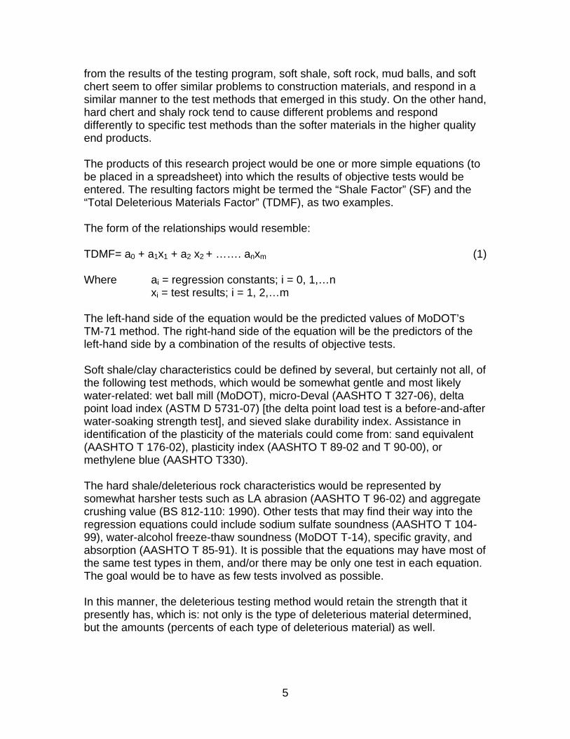
Because the objective of this study is to provide a system of tests to estimate deleterious materials as used by MoDOT TM-71, the test methods that MoDOT already specifies will not be part of the estimation system. These methods are Flat and Elongated, Minus #200 Sieve, and Organic Impurities. The primary deleterious materials sensitive to water are clay-bearing materials, such as mud balls, shale, shaly rock, “cap+20%”, and to a lesser extent, soft rock and some forms of OFM. Materials sensitive to handling and crushing would be weak materials, which include most of the deleterious materials discussed above. Thus, it may be necessary to include several types of tests for predicting each of the nine types of deleterious materials (Table 1). During the course of the study it became apparent that several of the nine types could be combined, such as is already done for “deleterious rock”. MoDOT may want to consider simplifying the assignment of deleterious types across the five types of aggregate products (MoDOT Standard Specifications sections 1002-1007). Looking at Table 1, and

5

from the results of the testing program, soft shale, soft rock, mud balls, and soft chert seem to offer similar problems to construction materials, and respond in a similar manner to the test methods that emerged in this study. On the other hand, hard chert and shaly rock tend to cause different problems and respond differently to specific test methods than the softer materials in the higher quality end products. The products of this research project would be one or more simple equations (to be placed in a spreadsheet) into which the results of objective tests would be entered. The resulting factors might be termed the “Shale Factor” (SF) and the “Total Deleterious Materials Factor” (TDMF), as two examples. The form of the relationships would resemble: TDMF= a0 + a1x1 + a2 x2 + ……. anxm (1) Where ai = regression constants; i = 0, 1,…n

xi = test results; i = 1, 2,…m The left-hand side of the equation would be the predicted values of MoDOT’s TM-71 method. The right-hand side of the equation will be the predictors of the left-hand side by a combination of the results of objective tests. Soft shale/clay characteristics could be defined by several, but certainly not all, of the following test methods, which would be somewhat gentle and most likely water-related: wet ball mill (MoDOT), micro-Deval (AASHTO T 327-06), delta point load index (ASTM D 5731-07) [the delta point load test is a before-and-after water-soaking strength test], and sieved slake durability index. Assistance in identification of the plasticity of the materials could come from: sand equivalent (AASHTO T 176-02), plasticity index (AASHTO T 89-02 and T 90-00), or methylene blue (AASHTO T330). The hard shale/deleterious rock characteristics would be represented by somewhat harsher tests such as LA abrasion (AASHTO T 96-02) and aggregate crushing value (BS 812-110: 1990). Other tests that may find their way into the regression equations could include sodium sulfate soundness (AASHTO T 104-99), water-alcohol freeze-thaw soundness (MoDOT T-14), specific gravity, and absorption (AASHTO T 85-91). It is possible that the equations may have most of the same test types in them, and/or there may be only one test in each equation. The goal would be to have as few tests involved as possible. In this manner, the deleterious testing method would retain the strength that it presently has, which is: not only is the type of deleterious material determined, but the amounts (percents of each type of deleterious material) as well.

6

RESEARCH PROJECT AGGREGATE TESTING

Researchers from Missouri S&T were to perform aggregate testing on a variety of aggregates, chosen by MoDOT to reflect a range in quality and use. The experimental testing plan was limited in scope to include three different MoDOT Section 1000 materials (1002, 1005, 1007), with three different ledges per aggregate-use type, along with two aggregate levels of quality. These two levels of quality would be represented by 1) the as-delivered condition and 2) the as-delivered amount of deleterious augmented by some additional deleterious material seeded into the aggregate to achieve a lower quality level. Each of the nine aggregates were to be subjected to a battery of aggregate tests (as presented above), and the results were to be used to produce the prediction equations.

MoDOT CONTRIBUTION

MoDOT personnel were to sample the production stone stockpiles from each ledge and blend the replicate bags of material prior to delivery. MoDOT personnel were to perform the TM-71 deleterious materials tests and report the results to Missouri S&T researchers. MoDOT was also charged with supplying deleterious material specific to each ledge. Other historical data associated with the materials was to be supplied.

POTENTIAL PROBLEMS

Because the final prediction system may include test methods for which MoDOT does not currently have data, then it is possible that no verification of the prediction model could occur. Verification (and possible model adjustment) would have to come after implementation of the new test methods by MoDOT. A second problem may be that some of the MoDOT aggregate specifications limit certain deleterious materials, such as shale content, to very small amounts. The threshold levels may be too low for detection by the aggregate test methods to be used in this study. A third problem could be that some of the parent aggregate may not have certain deleterious materials associated with it.

7

OBJECTIVE

The objective of this study is to establish a replacement of the existing MoDOT TM-71 deleterious materials method with a more objective system of test methods which would cover the various controlling behavior factors that the TM-71 method represents.

8

LITERATURE REVIEW

DELETERIOUS MATERIALS Deleterious materials are defined as materials that are extraneous to the parent material and diminish the optimum use of the aggregate product. Examples are shale, clay balls, soft rock, coal, lignite, wood, organic matter, minus #200 sieve material, soft chert, hard chert, and anything that would fall under the category of lightweight pieces. The literature contains numerous references to the negative action of various deleterious materials (Lang, 1931; Swenson and Chaly, 1956; Bloem, 1966). It has been shown that small amounts of deleterious material can result in poor performance even for aggregates with good field performance (Marks and Dubberke, 1982). “Deleterious material” is a relative term. A certain type of material at a certain content may be deleterious in some applications but not so in others. Due to the limited scope of the present project, deleterious materials not included in the following discussion include those that cause harmful chemical reactions and unsightly staining and efflorescence, such as organic impurities, soluble alkalis, reactive silica, and iron compounds, or have poor particle shape characteristics. These types of deleterious materials are handled by other MoDOT specified tests and policies, so they will not be considered below.

DELINEATION OF DELETERIOUS MATERIALS There have been a number of attempts to organize deleterious materials into systems (Lang, 1938; Walker and Bloem, 1950; Swenson and Chaly, 1956). Three types have emerged; each of the three is based on one of the following: 1) type of deleterious material, e.g. shale, 2) effect on PCC, HMA, or UAB, such as freeze/thaw damage, and 3) characteristics of aggregates that adversely affect the PCC, HMA, or UAB, such as toughness. MoDOT’s present system (TM-71) delineates the type of deleterious material. A common way in which deleterious materials are controlled is to prescribe certain test methods, then compare results to published acceptance limits (such as AASHTO M 80) for various classes of deleterious materials. Typical AASHTO test methods include clay lumps and friable particles (T 112), coal and lignite (T 113), low specific gravity chert (T 113), and material finer than #200 sieve (T 11). Other test methods relate to both deleterious materials and to the parent material. Examples of these methods are those that quantify toughness (Los Angeles abrasion T 96), soundness (sulfate soundness T 104), and absorption (T 85). Usually, deleterious materials fare worse in toughness and soundness tests than the parent rock, thus these methods can also be used for delineation of deleterious materials. The method used by MoDOT is MoDOT TM-71, which is a visual examination of particles, a rudimentary form of a petrographic analysis. Had some other method of delineation of deleterious materials been used in this

9

study, the prediction of deleterious materials would probably show different results in the relative importance of different aggregate test methods. Various deleterious actions and some commonly associated identifying test methods (as presented in the Introduction of this report) are discussed below.

DELETERIOUS ACTIONS

Impact and Abrasion Action Deleterious action by impact and abrasion of aggregate can occur during handling, stockpiling, bin loading, hauling, mixing, and abrasion across abutting pavement cracks and joints. Particles rubbing against each other or impacting each other or other objects can break down loose or unbound aggregate, changing gradation and increasing fines content, thus decreasing concrete and asphalt mixture workability, decreasing the ability to entrain air in concrete, and causing a loss of stability in aggregate base materials (Gray, 1962; Krebs and Walker, 1971; Folliard and Smith, 2003; Rangaraju and Edlinski, 2008). Abrasion from tire wear of concrete slabs and asphalt pavements can result in loss of surface texture and skid resistance (Senior and Rogers, 1991). The ability to resist impact and abrasion is referred to as toughness. Several test methods have been examined for characterization of toughness, such as Los Angeles abrasion, micro-Deval, wet ball mill, and sieved slake durability (Krebs and Walker, 1971; Richardson, 1985; Senior and Rogers, 1991, Saeed et al., 2001; Cooly and James, 2003; Meininger, 2004; Meininger, 2006; Rangaraju and Edlinski, 2008). Friable particles are subject to impact, resulting in breakdown into smaller particles or even a contribution to fines content. Soft particles are different—they are more prone to just abrasion (Forster, 2006). The following methods are considered tests of impact and abrasion.

Los Angeles Abrasion The Los Angeles Abrasion (LAA) test (AASHTO T 96) involves a two-fraction coarse aggregate specimen in a dry state being subjected to impact and abrasion by tumbling steel balls and aggregate particles inside a revolving drum (AASHTO, 2002). Resistance to impact and abrasion is called toughness. Toughness, as measured in the LAA method, is related to asphalt pavement stability (Krebs and Walker, 1971) and concrete aggregate resistance to degradation (Meininger, 2006) although the results of the test do not correlate directly with field performance (Krebs and Walker, 1971; Senior and Rogers, 1991). Some authors consider the LAA as both an impact and abrasion test (Cooly and James, 2003), while others felt it is mainly an impact test (Senior and Rogers, 1991; Rangaraju and Edlinski, 2008). It has been observed that sometimes weaker materials can actually exhibit lower losses due to their ability to absorb impact through elastic accommodation and that deteriorated material in the drum may also absorb some of the impact (Meininger, 2006). Also, the lack

10

of water in the test method may lead to poor field performance correlation because of the lack of interaction of impact/abrasion and water sensitivity (Senior and Rogers, 1991). In a review of aggregate test methods, LAA was evaluated as having merit in prediction of aggregate breakdown, but was limited in prediction of PCC pavement performance (Folliard and Smith, 2003). Eighty percent of the state DOT’s have LAA recommended limits for HMA of 40-45 percent loss (Kandhal and Parker, 1998). AASHTO M 80 limits LAA to 50 for PCC aggregates (AASHTO, 1999). MoDOT limitations are 50 for HMA aggregates, PCC crushed stone, and seal coat (section 1003) aggregates; 45 for PCC gravels; 55 for bituminous surface blade (section 1004) materials, and 60 for unbound surface (section 1006) aggregate (MoDOT, 2004).

Micro-Deval The micro-Deval (MD) test (AASHTO T 327) subjects a coarse graded material to revolving in a drum with steel balls (AASHTO, 2006), but the action is mainly abrasion, not impact (Cooly and James, 2003; Rangaraju and Edlinski, 2008). Also, because water is present, the MD test is also a measure of a material’s sensitivity to water and is related to weatherability. So, the test should be applicable to HMA, unbound base, and PCC aggregates. The test is purportedly more applicable to field performance than the LAA method, such as wearing of aggregate from tire wear (Senior and Rogers, 1991). The MD method has been shown to have a greater precision than LAA (Senior and Rogers, 1991). Several studies have shown that a strong correlation between MD and LAA does not exist (Kandhal and Parker, 1998; Cooly and James, 2003; Meininger, 2004; Rangaraju and Edlinski, 2008). It has been postulated that grading of the aggregate specimen is more important to MD than LAA (Rangaraju and Edlinski, 2008). Strong correlations have been found between MD and magnesium sulfate soundness and wet ball mill by some (Kandhal and Parker, 1998; Jayawickrama et al., 2001) while others have disagreed (Meininger, 2004). The MD method was selected as a superior test for evaluation of granular base, asphalt mixture, and portland cement concrete aggregates (Senior and Rogers, 1991; Kandhal and Parker, 1998; Saeed, et al., 2001; Folliard and Smith, 2003; Meininger, 2004; White et al., 2006). Recommended limits for HMA surface and binder courses of 17 and 20, respectively, have been reported (Kandhal and Parker, 1998). A level of 15 percent loss has also been suggested for HMA (White et al., 2006). For unbound granular base, Saeed et al. (2001) proposed a sliding scale of MD threshold values based on traffic level, moisture availability, and frost action. For an area of high moisture availability and frost potential, the maximum MD value for medium and high traffic levels was 5; for low traffic: 15; for less severe conditions: up to 45.

11

Wet Ball Mill

The wet ball mill (WBM) test (Tex-116-E) is similar to an LAA test with the addition of water (TexDOT, 2000). Thus, all three destructive factors discussed above are present: impact, abrasion, and water’s contribution to both actions. The WBM method was developed as a test method for assessing aggregate for base material. The wet ball mill test method has been in use for aggregate quality testing in various forms for a number of years and for a variety of aggregate end-use purposes, including railroad ballast. Various designations include Mill Abrasion (Clifton et al., 1987; Clifton et al., 1987(2); Selig and Boucher, 1990; UP&BNSFR, 2001) and Texas Wet Ball Mill (Texas DOT, 2000). A good correlation has been found between MD and WBM. However, the method has exhibited greater precision than the MD method (Jayawickrama et al., 2001). One state’s recommended upper limit for granular base is 55 percent loss (Texas DOT, 2000).

Sieved Slake Durability

The sieved slake durability (Isd2) test was adapted from ASTM D 4644 to rate shale for applicability as embankment, subgrade, and subbase materials in regard to durability (Richardson, 1984; Richardson, 1985; Richardson and Long, 1987). The test involves the tumbling of particles in a mesh drum in water, with a subsequent evaluation of degradation via a sieve analysis. The action mainly involves sensitivity to water, but there is some abrasive action, thus the method’s inclusion in this section. Isd2 values of shale have been reported to range from 2 to 90 percent (Richardson, 1984).

Crushing/Cracking During Loading Action Another destructive action on aggregate that is similar to impact and/or abrasion is a crushing action under static or dynamic load, such as the weight of a stockpile or the compactive effort during construction. Cracking action could occur during service loading of a concrete structure. Breakdown of loose aggregate is somewhat a function of particle shape, where a more elongated angular shape tends to break more easily. Also, a more well-graded aggregate will break down less easily because of the support offered by the smaller particles. Like impact and abrasion, crushing results in a finer gradation and a reduction in desired physical properties (Gray, 1962; Senior and Rogers, 1991; Lade et al., 1996). In concrete, shale and soft sandstones have resulted in significant losses of strength (Lang, 1927; Emmons, 1930; Walker and Bloem, 1950; Dolar-Mantuani, 1978; Richardson and Whitwell, 2009). Two test methods are thought to represent the action of aggregate under static or dynamic loading: aggregate crushing value and the point load strength.

12

Aggregate Crushing Value

The aggregate crushing value (ACV) was developed as a standard aggregate quality test (BS 812, 1990) in Britain for a variety of aggregate end-uses. The aggregate crushing value test method (British Standards Institution BS 812: Part 110) consists of subjecting a compacted specimen of aggregate particles to a static load, then measuring the amount of breakdown (BSI, 1990). The aggregate particles bear on each other and are subjected to point contact loads (thus to an indirect tensile load) as well as abrasion action as the particles slide past each other. Being subjected to internal tensile loading would make the test a measure of both tensile strength and elastic response to load. ACV results correlate well with Los Angeles abrasion results (BSI, 1998; Kandhal and Parker, 1998; Saeed et al., 2001; Williamson et al., 2007). Saeed et al. (2001) have found a fair correlation of ACV with MD. Rodgers et al. (2000) have found good correlation of the ACV with field performance of unbound aggregate pavement surfaces. They also noted additional degradation when the test was performed wet as opposed to dry. It has been singled out as a good measure of the strength of aggregate in a graded aggregate setting (Folliard and Smith, 2003). The recommended ACV limit for HMA of 30 percent loss has been reported by Kandhal and Parker (1998).

Point Load Strength Crushing at a local level within an aggregate particle relates to tensile strength. The measurement of tensile strength of geologic materials has seen several approaches. One is the indirect tensile strength test, also known as the Brazilian test. In this method, a rock core (or concrete cylinder or asphalt puck) is placed on its side with a line load applied diametrically. The Point Load Index test (ASTM D 5731-07) was developed as a quick test method to estimate the indirect tensile strength of rock cores (ASTM, 2007). It is similar to the indirect tension method, but instead of applying a line load, a point load is used. This allows a smaller load and thus a smaller, simpler loading device. Specimens can also be loaded axially; likewise, irregular lumps can be tested (Broch and Franklin, 1972; Bieniawski, 1975). Major advantages of the method include the ability to test irregular lumps, a small load frame requirement, and quickness of testing, resulting in a potential for testing a larger number of specimens. Specimen size affects the outcome, so the results need to be converted to a standard equivalent size (typically 50 mm). Strength decreases as specimen size increases (Hardin, 1985; Richardson, 1989; McDowell and Bolton, 1998; Lade et al., 1996). ASTM D 5731-07 recommends testing specimens no smaller than 30 mm, primarily to assure that the specimen fails in tension rather than compression (ASTM, 2007). One study showed that even for specimens less than 10 mm, results were valid as long as the specimens failed in tension, as opposed to crushing. This concept works for harder aggregates (Lobo-Guerrero and Vallejo, 2006). The point load strength (PLS) has been used to evaluate the durability of shale (Richardson, 1985).

13

Swelling/Shrinkage and Breakdown from Wetting/Drying

Shale, clay lumps, coal, and lignite are known to be sensitive to wetting and drying cycles. Disintegration in bases, subbases, and subgrades can cause loss of strength and possible swelling, resulting in the loss of stability in pavement structures. Durability rating systems for shale have been developed (Richardson, 1984; Richardson and Wiles, 1990). Shale, clay lumps, coal, and lignite also disintegrate or swell in concrete slabs or even asphalt pavements, leading to popouts and pitting, or micro-cracking of concrete (Forster, 2006). Unfortunately, it has been found that creation of specifications to control damage from shale has met with limited success due to the wide variation in shale characteristics (Walker and Proudley, 1932). Because shale and other types of soft rocks fail by different mechanisms, a wide variety of tests have been utilized to assess susceptibility to degradation in the presence of water. Among these are the sieved slake durability index, wet ball mill, micro-Deval, plasticity index (PI), sand equivalent (SE), methylene blue (MB), and delta point load strength. MB values have been linked to degradable aggregate (Bjarnason, et al., 2000). The sieved slake durability, wet ball mill, and micro-Deval methods have been discussed earlier. Clay content and activity have been shown to relate to the durability and swelling characteristics of shale (Richardson, 1984), thus, measures of clay characteristics could have some correlation with deleterious action. Typical tests that would represent this sort of activity would include PI, sand equivalent, and methylene blue. These will be discussed in more detail later in the report.

Delta Point Load Strength The aforementioned point load test can be performed on both dry and wet specimens. The difference between the dry and wet strengths is called the delta point load strength (ΔPLS). The ΔPLS test method was developed to quantify the loss in strength from soaking. As ΔPLS increases, durability has been shown to decrease. Hard shales of intermediate durability have exhibited ΔPLS values as low as 13 percent (Richardson and Wiles, 1990).

Freeze/Thaw Action Deleterious particles in concrete can lead to several types of distress, including popouts from hard chert, pitting from softer materials, map cracking and D-cracking (Krebs and Walker, 1971). Walker and Bloem (1950) identified deleterious materials in this regard to include porous chert, weathered rock, laminated rock, argillaceous rock, and shale. As little as a five percent content of certain soft stones and shale caused significant losses of freeze-thaw durability.

14

Walker and Proudley (1932) also included chert as a deleterious material, and rated shale and chert as the most deleterious to concrete. Lang (1931) divided deleterious materials into those that undergo volume change (shale and certain cherts), and those that were soft or weak. Aggregate expansion can caused D-cracking damage to concrete, and popouts in both concrete and asphalt pavements. Freezing/thawing action also broke down aggregate in stockpiles, leading to the above-mentioned problems of increased fines and changed gradation. Poor performance of inferior aggregate (deleterious) materials has been linked to the particle’s pore characteristics, elastic accommodation, and mineralogy (Verbeck and Landgren, 1960). These three factors are discussed in the next section.

Pore Characteristics

Pore characteristics include pore size, distribution, and shape. Pore size and distribution relates to permeability, the ability of water to enter and pass out of aggregate particles. Pore shape affects the ease of which water can escape a pore. A variety of aggregate properties and associated test methods have been used for assessment of aggregate frost susceptibility, including absorption, bulk specific gravity, and soundness tests: water-alcohol freeze-thaw soundness and sulfate soundness. Tests that relate to pore characteristics are presented below.

Absorption

Absorption, typically measured by AASHTO T 85 (AASHTO, 2000), has been considered a viable indicator of frost susceptibility. It typically is one of the better stand-alone tests for correlation with durability, although the correlation is not high. However, the test is easily and commonly performed (Dolch, 1966; Senior and Rogers, 1991). Aggregates with low absorption (less than 0.3%) frequently show acceptable resistance to frost damage. Upon exposure, there is insufficient water available to cause damage. However, absorption does not accurately measure the ease of water entry and exit as affected by pore shape and distribution. It has been postulated that a more accurate assessment would come from a combination of absorption and permeability (Dolch, 1959). Others have found a good correlation between absorption and AASHTO T 161 Method B “Resistance of Concrete to Rapid Freezing and Thawing” (AASHTO, 2000). Absorption values less than 1.5 percent indicated durability factors (DF) greater than 75, while absorptions greater than two percent were associated with inferior DFs (Koubaa and Snyder, 1996; Richardson, 2009). There are highly porous aggregates that exhibit good durability during freezing and thawing because of large pores that drain easily (Cordon, 1948).

15

MoDOT absorption percent limits are: 1) for HMA: 4.0 for crushed stone and 5.5 for gravel, 2) for PCC crushed stone (paving): 2.0, 3) for PCC masonry: 3.5 for crushed stone and 4.5 for gravel, 4) section 1003: 6.0, and 5) for section 1004: 7.0 (MoDOT, 2004).

Bulk Specific Gravity

Bulk specific gravity (BSG), also determined in AASHTO T 85, is a function of internal porosity and mineralogy (specific gravity of the solids). Traditionally, it has been thought that absorption is the more direct indicator of freeze-thaw susceptibility compared to specific gravity, and because the two are correlated and in fact are values produced by the same test method, specific gravity has not been considered the primary parameter of the two. However, some studies have shown that for carbonate aggregates, a certain relationship exists between specific gravity and durability. Bulk specific gravities greater than 2.60 or 2.65 exhibited superior durability and had a good correlation with DF (Koubaa and Snyder, 2001; Harman et al., 1970; Richardson, 2009). Low specific gravity chert is limited in AASHTO M 80 to 3.0 percent for paving and bridge deck concrete (AASHTO, 1999). Low specific gravity (less than 2.40) has been associated with poor freeze-thaw resistance (Sweet, 1940). However, some aggregates with very low specific gravities (2.24-2.35) and large absorptions have been shown to be quite durable–a fact explained by a large diameter pore system, which prevented the build-up of pressure (Harman et al., 1970) and possibly a lower elastic modulus, allowing greater elastic accommodation. BSG has been found to be useful in prediction of T 161 DF via regression analysis (Richardson, 2009).

Vacuum Saturated Absorption

Subjecting aggregate to vacuum will increase the amount of absorption of water into pores that are more difficult to enter. Some studies have indicated that vacuum saturated absorption (VSAbs) correlates well with T 161 Method A for aggregates with either high or low DF values (Larson et al., 1965; Larson and Cady, 1969; Richardson, 2009). Others have shown that vacuum saturated absorptions of greater than two percent exhibit excessive dilation or reduction in transverse frequency during T 161 Method A testing (Harman et al., 1970; Williamson et al., 2007). VSAbs has been found to correlate better with both elastic accommodation tests (LAA, MD, ACV) and soundness tests. Of the three elastic accommodation tests, MD correlated best with VSAbs (Williamson et al., 2007; Richardson, 2009). VSAbs has been found to be useful in prediction of T 161 DF via regression analysis (Richardson, 2009). VSAbs has also been put forth as a primary screening test for aggregate durability (Williamson et al., 2007; Richardson, 2009).

16

In general, aggregates with intermediate values of absorption or vacuum saturated absorption (1.5 to 2.5 percent) are problematic in the predictive ability of frost susceptibility.

Vacuum Saturated Specific Gravity

Again, when the absorption of vacuum saturated aggregates is determined, vacuum saturated bulk specific gravity data is also generated. VSBSG has been found to correlate with T 161 results. VSBSG has been found to be useful in prediction of T 161 DF via regression analysis, and has also been suggested as a primary screening test for aggregate durability (Richardson, 2009).

Water-Alcohol Freeze-Thaw and Sulfate Soundness

Both water-alcohol freeze-thaw soundness (AASHTO, 2007) and sulfate soundness (AASHTO, 2003) testing involve water penetration into aggregate pores, thus, these methods involve an element of ease of water entry. The methods are discussed in more detail in a subsequent section.

Elastic Accommodation/Strength

Elastic accommodation is the ability of the particle to expand upon the onset of water freezing without fracture. Reaction can take the form of either sufficient strength to resist fracture, or elastic accommodation of the pressure. The ideal aggregate would have high tensile strength to resist stress due to expansion, but have a low modulus of elasticity to deflect elastically to accommodate the stress. A high Poisson’s ratio would prevent stress from being transmitted laterally in other directions, thus limiting stress (and limiting an increase in pore pressure) in pores in those directions (Verbeck and Landgren, 1960). Although reports have identified failure as a function of the stress exceeding the tensile strength (Powers, 1955; Verbeck and Landgren, 1960), attempts to quantify aggregate tensile strength in relation to aggregate freeze/thaw durability have not been reported. Unfortunately, high tensile strength and low modulus in brittle materials are usually mutually exclusive. Thus, interpretation of various test method results is difficult; e.g. does a high tensile strength result also indicate low elastic accommodation behavior, or not? Freeze/thaw-type tests that utilize aggregate in an unconfined state do not consider the effect of confinement by the concrete paste. The following are tests that reflect some aspect of the manner of the aggregate’s reaction to internal pressure.

17

Aggregate Crushing Value and Point Load Strength

Aggregate crushing value and point load strength test methods have been presented previously. Both methods have been found to be useful in prediction of T 161 DF via regression analysis (Richardson, 2009). Walker and Bloem (1950) reported that soft deleterious aggregate lowered concrete flexural strength and freeze/thaw resistance.

Los Angeles Abrasion

The LAA test method (AASHTO T 96) subjects the aggregate specimen to abrasion and impact loading (AASHTO, 2002). The impact portion could be considered as an indirect measure of tensile strength and elastic accommodation. Unfortunately, harder, stronger aggregates may exhibit lower LAA values because of a lack of accommodation of impact loading, thus, making interpretation of results difficult (Meininger, 1978). LAA results for flat and/or elongated particles are also open to interpretation (Woolf, 1966).

Micro-Deval

Degradation action in the micro-Deval (MD) test (AASHTO T 327) is primarily due to slaking and abrasion, but not impact, as in the LAA test (AASHTO, 2006). Thus, the MD test is limited in its ability to measure tensile strength or elastic accommodation important to freeze/thaw resistance. It does have merit for use as a general quality indicator. Several studies have shown that MD results correlate with service records of durability of asphalt aggregate (Wu et al., 1998a, 1998; Kandahl and Parker, 1998). There have been mixed results reported in the literature in regard to the correlation of MD with other toughness tests, such as LAA and ACV (Kandahl and Parker, 1998; Saeed et al., 2001; Wu et al., 1998b, 1998; Richardson, 2009). MD has been found to be useful in prediction of T 161 DF via regression analysis, and has also been suggested as a primary screening test for aggregate durability (Richardson, 2009).

Water-Alcohol Freeze-Thaw Soundness

It is difficult to decide under what category to place soundness testing, because soundness assesses: 1) the ability for water to enter the aggregate’s pore system, 2) the reaction to wetting, 3) the tensile resistance to expansion and hence to tensile stress (tensile strength and elastic accommodation), and even 4) interactions with the mineralogy of the aggregate. Various state DOTs and other agencies specify some version of the water-alcohol freeze-thaw soundness method (Forster, 2006). The AASHTO T 103 Water-Alcohol Freeze-Thaw (WAFT) method (AASHTO, 2000) has not been shown to have a strong relationship with frost resistance (Thompson et al., 1980; Mindess et al., 2003; Wu et al., 1998; Wu et al., 1998), and does not correlate

18

particularly well with other soundness tests (Rogers, 1989; Hossain et al., 2007). However, it has been shown to have better precision than other soundness tests (Rogers, 1989). Also, it has been shown to correlate with durability better than sulfate soundness (Brink, 1958). Used in concert with either absorption or MD, WAFT has been successful at identifying marginal aggregates (Senior and Rogers, 1991). It has been noted that the degree of saturation during WAFT testing is important. Non-uniform saturation can explain the lack of agreement between WAFT results and service performance records. It was recommended that 85 percent saturation be achieved via one hour of evacuation followed by 23 hrs. of immersion prior to freeze-thaw testing (Sweet, 1940). MoDOT’s TM-14 (2007) is a hybrid of AASHTO T 103 methods B and C (MoDOT 2007). Method B correlates best with service records. MoDOT percent limits for various applications are PCC: crushed stone (paving): 16.0; and for masonry (crushed stone or gravel): 18.0 (MoDOT, 2004). Former specifications limited TM-14 to 10.0 percent for Gradation F (D-cracking prone) materials.

Magnesium and Sodium Sulfate Soundness

Probably the most commonly specified soundness test is one of the two versions of AASHTO T 104 sulfate soundness, using either magnesium or sodium sulfate (AASHTO, 2003). Like WAFT, the method employs an artificially-induced expansion, with failure measured as a change in gradation of the fabricated gradation. Thus, sulfate soundness could be considered a measure of tensile strength or elastic accommodation. Sodium sulfate soundness (NaSO4) has been found to be useful in prediction of T 161 DF via regression analysis, and has also been suggested as a primary screening test for aggregate durability (Richardson, 2009). Maximum recommended limits for sodium sulfate soundness as applied to HMA are 11 to 15 percent (about 60 percent of state DOTs) and 25, 30, and 10 percent for Methods A, B, and C, respectively for T 103 (Kandhal and Parker, 1998). Several studies have indicated a preference of magnesium sulfate soundness over sodium sulfate soundness (Kandhal and Parker, 1998; Saeed et al., 2001; White et al., 2006). Sulfate soundness has not been shown to be an accurate predictor of frost susceptibility in PCC aggregates, either from slow cooling testing or service records. Several reasons for this include the difference in destructive mechanisms and the lack of precision of the methods (Walker and Proudley, 1932; Swenson and Chaly, 1956; Harman et al., 1970; Marks and Dubberke, 1982; Cady, 1984).The method also does not correlate well with WAFT (Brink, 1958). Some studies have reported mixed success in prediction (Paxton, 1982; Chamberlain, 1981), while in others, magnesium sulfate soundness (MgSO4) has been recommended as a preferred method for relating to HMA raveling, potholes, and popouts (Kandhal and Parker, 1998), and for unbound granular

19

base (Saeed et al., 2001). Magnesium and sodium sulfate methods do not necessarily agree. Magnesium sulfate is sometimes preferred to sodium sulfate because the solubility of the magnesium salt is less sensitive to temperature than the sodium salt, and the MgSO4 crystals are more uniform, thus, MgSO4 soundness results tend to be less erratic (Walker and Proudley, 1932). In general, sulfate soundness prediction of freeze-thaw durability has had mixed success, and the method suffers from imprecision. Soundness has been shown to correlate better with MD than LAA does with MD (Cuelho et al., 2007). For unbound granular base, Saeed et al. (2001) proposed a sliding scale of MgSO4 threshold values based on traffic level, moisture availability, and frost action. For an area of high moisture availability and frost potential, the maximum MgSO4 value for medium and high traffic levels was 13 percent loss; for low traffic: 30; for less severe conditions: up to 45. A level of 20 has also been suggested for HMA (White et al., 2006). For PCC aggregate, AASHTO M 80 limits loss by NaSO4 and MgSO4 to 12 and 18 percent, respectively.

Wet Ball Mill

The wet ball mill (WBM) test method is similar to the LAA test in that aggregate is subjected to impact and abrasion by steel balls picked up on a shelf and dropped in a rotating drum plus the impact and abrasion from other aggregate particles (TexDOT, 2000). The method is similar to the micro-Deval test in that water is also present. The testing action suggests that the results could be used as a measure of tensile strength and elastic accommodation, as well as the resistance to water-induced reduction of aggregate strength. WBM results have been found to be useful in prediction of T 161 DF via regression analysis, and the method has also been suggested as a primary screening test for aggregate durability (Richardson, 2009).

Mineralogy

Trypolitic chert in carbonate aggregate has caused aggregate to disintegrate while undergoing T 161 freeze/thaw testing (Dubberke, 1983). Clay minerals are known to increase water demand in concrete, induce stripping in HMA, and lower stability of unbound granular base material. In a comparison to illites and kaolinites, smectites are the most damaging, having a greater fineness and surface activity.

Asphalt-Aggregate Bond Interference Deleterious materials, in the form of dust or coatings, can interfere with the bond between asphalt binder and aggregate particle surfaces. Thus, stripping of binder can be the result. Presence of clay can also cause spontaneous emulsification, another cause of stripping (Stuart, 1986; Kandhal, 1992; Kandhal et al, 1998).

20

The following test methods relate to asphalt-aggregate bond interference.

Plasticity Index The PI test method involves several test designations: MoDOT TM-79 (MoDOT, 2004), AASHTO T 89 (AASHTO, 2002) and T 90 (AASHTO, 2000). FHWA Technical Advisory T5040.27 (1988) indicated that the presence of clay fines can contribute to stripping. It was recommended that aggregate information in the mix design report should include PI and sand equivalent (SE) values. Suggested limits on SE and amount of deleterious material (clay lumps and friable particles) were given. Both ASTM D 1073 (Standard Specification for Fine Aggregate in Bituminous Paving Mixtures) and D 242 (Standard Specification for Mineral Filler for Bituminous Paving Mixtures) limit the PI of the minus #40 fraction of material used in bituminous mixtures to a maximum of 4. For mineral filler, most state DOTs reference AASHTO M17, which specifies a maximum PI limit of 4. A survey that targeted state DOTs that use limestone in hot mix asphalt conducted by the Missouri Limestone Producers Association (MLPA) revealed that about half the responding DOTs specified a limiting value for PI (MLPA, 2001). Kandhal and Parker (1998) stated in their literature review that a reported correlation between PI and field performance of HMA could not be found in the published literature. However, they recognized the PI is determined for materials that contain minus #40 to plus #200 material and that PI limits should be developed just for material passing the #200. The study indicated that little research has been done relating PI of minus #200 and HMA performance. There is a contention that a material can show plastic properties in the absence of clay content. The report also stated that the liquid limit (LL) and plastic limit (PL) tests are subjective and based on the experience of the tester. In a study of 10 fine aggregates, four of which were seeded with clay, Kandhal et al. (1998) evaluated the PI, sand equivalent, and methylene blue methods by comparing to results of AASHTO T 283 (AASHTO, 2003) and the Hamburg Wheel-Tracking Device (HWTD). Upon testing the minus #40 material, all 10 aggregates were non-plastic; however, when testing the minus #200 material, five were considered to be highly plastic. In almost all cases, those sands with high PI values for the minus #200 material were the worst performers in both the T 283 and HWTD results. MoDOT (2001) has stated that its position on PI is that each aggregate fraction of a common ledge (source) should be tested separately rather than as a blend because the coarser (gritty) size materials will not allow a thread to be rolled, yet there could be deleterious material present which could cause stripping. For granular base material, Gray (1962) has shown that there is a three percent loss in triaxial shear strength per one percent increase in PI. MoDOT’s percent limits for granular base (section 1007) materials are 6 or 8 depending on the type of unbound base (MoDOT, 2004).

21

Sand Equivalent

Hveem (1953) developed the sand equivalent (SE) method as a rapid field correlation test to assign a relative amount, fineness, and character of clay-like material in an aggregate sample. Other states were quick to recognize the value in substituting the SE for the more time-consuming traditional PI-and-minus #200 combination as a field test (O’ Harra, 1955). The SE method is AASHTO T 176 (AASHTO, 2002) and ASTM D2419 (ASTM, 2002). The SE is a rapid, simple test to perform requiring minimal equipment, training and experience (Kandhal and Parker, 1998). Hveem (1953) and Clough and Martinez (1961) showed that SE decreases with increasing amounts of dust and increasing activity of the dust. However, Gaynor (1968) found little correlation between SE and percent minus #200 material. Hveem also noted a decrease in SE with increasing fineness of dust. FHWA T5040.27 recommended a minimum of 45 percent for the SE (1988). For cleanliness assurance, the 1994 Superpave methodology recommended various levels tied to design traffic which MoDOT has adopted for HMA (MoDOT, 2004). Various studies have indicated that the SE test method is promising in regard to prediction of HMA moisture sensitivity. Clough and Martinez (1961) used specially prepared asphalt mixtures seeded with different types of fines. They found a good correlation between SE and immersion-retained Marshall stability and visual stripping test results. Aschenbrener (1992) also indicated that the SE has a good correlation to HMA resistance to stripping and moisture sensitivity. Kandhal et al. (1998) also found a relationship between SE and T 283 and HWTD results. However, Cross and Voth (2001) did not find a significant correlation between SE, MB, T 283, or Asphalt Pavement Analyzer (APA) rut depths. Heidebrecht (1964) did not find a significant correlation between SE and PI, but asserted that this may have been due to the differing amounts of minus #200 in the test specimens. Studies have shown a relationship between SE and water demand in concrete mixtures (Dolar-Mantuani, 1966). In regard to concrete, Buth et al. (1967) report that a decrease in SE of 20 percent resulted in a corresponding 16 percent loss of strength and an increase in shrinkage of 15 percent, although there was no change in durability. MoDOT has reported that because SE does not require a pre-soak, the test method does not adequately identify “shale” content (MoDOT, 2001). Lusher (2004) has pointed out the difficulties in interpreting the results of an angular, coarse graded material. MoDOT percent limits for Superpave HMA vary from 40 to 50, depending on traffic load (MoDOT, 2004).

22

Methylene Blue

There are several methods for estimation of the amount and nature of deleterious materials such as clay and organic matter. One of the simplest is AASHTO T 330, the methylene blue test (AASHTO, 2007). Methylene blue is a cationic dye that is adsorbed by clay surfaces due to cationic exchange; the test is really a measure of the cation exchange capacity of the material, and is an indication of surface activity. The MB method measures the amount and nature of potentially detrimental material: greater MB means more clay and/or clay with greater activity. In regard to type of rock, igneous rocks tend to have greater MB values due to the montmorillonite (smectite) content (Kandhal and Parker, 1998). There is evidence that the MB test can be used to assess strength reductions in concrete due to the presence of various clay types (Pike, 1992; Yool et al., 1998). The International Slurry Seal Association recommends the methylene blue test for quantifying the amount of clays, organic matter, and iron hydroxides in fine aggregate (ISSA, 1989). Kandhal and Parker (1998) correlated both SE and MB results with T 283 and HWTD results and found that the MB method had a greater correlation than SE. The recommendation was to replace PI and SE with MB for control of stripping of HMA. However, White et al. (2006) reported poor stripping predictability by MB because of a poor/fair correlation with T 283 results. Aschenbrener and Zamora (1995) also found that the MB correlated better to T 283 and field performance than the SE. Although Cross and Voth (2001) did not find a significant correlation between MB, SE, T 283, or APA rut depths, they recommended MB as a supplementary test. Bjarnason et al. (2000) have found MB to be useful in quantification of deleterious fines, which indicated aggregate that is prone to breakdown. Yool et al. (1998) warn that the MB results are not in proportion to the damaging effects on concrete. The damage ratio is less than the MB ratio of the material. MoDOT has stated (2001) that the MB method gives inconsistent results, and is problematic in that there is no pre-soak requirement. It is recommended that in addition to a dry shaken material, the adherent fines should also be tested (Kandhal and Parker, 1998).

Cement-Aggregate Bond Interference

As with asphalt mixtures, a key factor that affects concrete properties is the bond between the cement paste and the aggregate. Interference by dust (Pike, 1992; Gullerard and Cramer, 2003; Richardson and Whitwell, 2009) and coatings (Goldbeck, 1932; Buth et al., 1964; Shah and Chandra, 1968; Darwin and Slate, 1970; Dolar-Mantuani, 1978; Schmitt, 1990; Popovics, 1998; Richardson and Whitwell, 2009) can lower the bond strength, and in turn, lower the strength of the concrete. Goldbeck reports losses of 1.5 to 2.0 percent per one percent dust.

23

The action of fines is a function of the amount and nature of them. A small amount of non-plastic fines may actually enhance the properties of the concrete. The strength of the bond to the aggregate can best be determined by strength tests of the concrete, plus a post-test examination (Forster, 2006).

Water Absorption by Highly Plastic Fines

Absorption of water by highly plastic fines will increase the water demand of concrete mixtures, which lowers the workability due to both the activity of their surfaces and their extremely fine nature (Yool et al., 1998). The MB value increases with increasing fines content and hence will cause greater water demand (Stewart et al., 2007). If the water demand is satisfied by the addition of water, strength will decrease: there was an inverse relationship between liquid limit and both compressive strength and modulus of rupture (Buth et al., 1964), and between MB and compressive strength (Stewart et al., 2007). Satisfaction of water demand also lowers durability and increases shrinkage potential. A more plastic material will cause greater problems: e.g. as the montmorillonite (smectite) content increases, there will be more swelling (Swenson and Chaly, 1956). Pike (1992) reported ratios of percent strength loss per increase in MB for kaolinites, illite, and smectite as follows: 1:1, 2:1, and 4:1, respectively.

Clay Lubrication

Presence of clay in aggregate base material and asphalt mixtures can cause a loss of stability, with the type and volume of the clay being the main factors (Hveem, 1953; MoDOT, 2001). As PI increases, triaxial shear strength decreases (Gray, 1962).

SYSTEM ESTIMATION OF AGGREGATE DELETERIOUS MATERIAL CONTENT

The estimation of construction aggregate durability has been successfully accomplished for low quality select material, mainly used for embankment and highway subbase material. The approach was to rate durability in terms of loss of shear strength upon wetting, then approximate the loss rating via a regression equation. The main effects in the regression equation were the results of numerous aggregate quality test methods (Richardson, 1984; Richardson, 1985; Richardson and Long, 1987; Richardson and Wiles, 1990). In a similar manner, T 161 DF of concrete has been predicted with regression of various aggregate test methods (Richardson, 2009).

24

SUMMARY

There are a variety of deleterious materials that cause problems in PCC, HMA, and UAB. Friable particles, such as weakly cemented sandstones and mud balls, are weak so they break down, creating fines or they stay intact and weaken the PCC, HMA, or UAB. Weak particles, such as some shales, coal and lignite, and clay lumps may also disintegrate and cause surface PCC and HMA pitting. Soft particles abrade, creating fines. “Soft” and “weak” do not necessarily mean the same thing. Unsound particles, such as chert and some shales, may be weak or not, but they expand upon freezing or wetting and cause disruptive forces, and end up being surface popouts in PCC and HMA or causing cracking in PCC. Friable, weak particles can be detected by impact tests, such as LAA and WBM, and by strength tests such as PLS and ACV. Soft particles can be identified by abrasion tests, such as LAA, WBM, MD, and perhaps ACV and Isd2. Soft and weak particles such as clay balls and shale may contain clay, and so may be identified by PI, MB, and SE. The greater the clay activity, the greater the detrimental effect. Unsound particles can be detected by soundness tests that cause expansive pressure, such as sulfate soundness and WAFT, or by methods that detect pore characteristics, such as Abs, BSG, VSAbs, and VSBSG. There will be some cross-over detection due to the correlation of behavior, such as MD and soundness or LAA and ACV. Within these subsets of behavior, some tests correlate well with each and some do not. Sometimes the literature reports mixed results. Expectations are:

LAA correlates well with ACV and VSAbs, but just fair with MD. LAA does not correlate well with pavement performance. Impact tests can be “fooled” by some soft but resilient materials

MD may correlate well with WBM and MgSO4 (or it may not), but just fair with ACV (or perhaps good), MD has better precision than LAA. MD is held up as a superior overall evaluation method.

ACV has been singled out as a good method for graded aggregate evaluation.

PLS is a simple way of assessing rock strength.

WAFT does not correlate well with NaSO4 or freeze-thaw tests WAFT in concert with other tests such as MD or Abs correlates well with pavement performance.

NaSO4 has poor precision. MgSO4 is considered a superior test to NaSO4

25

NaSO4 does not correlate well with pavement performance

VSAbs correlates well with Abs, LAA, MD, ACV, VSBSG, and BSG. Low BSG (less than 2.4-2.5) is usually associated with poor performance. High Abs (greater than 2-3 percent) is usually associated with poor performance.

PI, SE, and MB do not correlate well with each other, partly because of sample preparation differences. The SE procedure is flawed. The PI procedure is flawed.

Isd2 is a good test for shale durability.

26

TECHNICAL APPROACH

GENERAL

Experimental Design

The proposed testing matrix included three levels of material type, three different ledges per material type, and two levels of quality (unseeded and seeded), for a total of 18 sample types. Each of the 18 sample types was to be subjected to a battery of aggregate tests and the results used to produce the TM-71 predictive equation. Thus, the predictive regression equations would possibly contain one or more terms as determined from a suite of aggregate tests. This full factorial experiment (3x3x2) resulted in 18 different combinations.

Replicate Specimens Normally, three replicate specimens were tested per test method. The results were analyzed for precision and identification of outliers. The replicate test results were averaged before entry into the correlation and regression analyses.

MATERIALS MoDOT Construction and Materials (Physical Laboratory Central Laboratory) chose the specific aggregate materials. Sampling was performed by either MoDOT District or Central Laboratory personnel. Central Laboratory personnel delivered the bagged samples to the Missouri S&T Civil, Architectural, and Environmental Engineering (CArE) aggregate laboratory. The actual materials delivered are shown in Table 3.

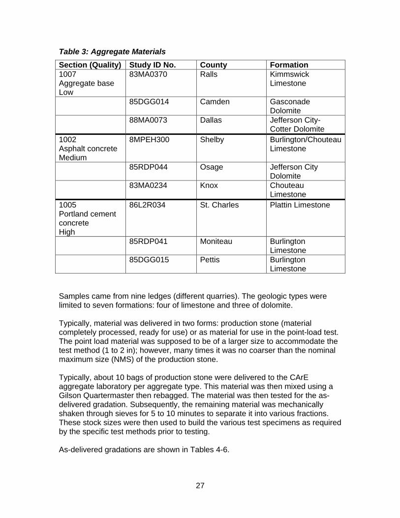
27

Table 3: Aggregate Materials

Section (Quality) Study ID No. County Formation 1007 Aggregate base Low

83MA0370 Ralls Kimmswick Limestone

85DGG014 Camden Gasconade Dolomite

88MA0073 Dallas Jefferson City-Cotter Dolomite

1002 Asphalt concrete Medium

8MPEH300 Shelby Burlington/Chouteau Limestone

85RDP044 Osage Jefferson City Dolomite

83MA0234 Knox Chouteau Limestone

1005 Portland cement

86L2R034 St. Charles Plattin Limestone

concrete High 85RDP041 Moniteau Burlington

Limestone 85DGG015 Pettis Burlington

Limestone Samples came from nine ledges (different quarries). The geologic types were limited to seven formations: four of limestone and three of dolomite. Typically, material was delivered in two forms: production stone (material completely processed, ready for use) or as material for use in the point-load test. The point load material was supposed to be of a larger size to accommodate the test method (1 to 2 in); however, many times it was no coarser than the nominal maximum size (NMS) of the production stone. Typically, about 10 bags of production stone were delivered to the CArE aggregate laboratory per aggregate type. This material was then mixed using a Gilson Quartermaster then rebagged. The material was then tested for the as-delivered gradation. Subsequently, the remaining material was mechanically shaken through sieves for 5 to 10 minutes to separate it into various fractions. These stock sizes were then used to build the various test specimens as required by the specific test methods prior to testing. As-delivered gradations are shown in Tables 4-6.

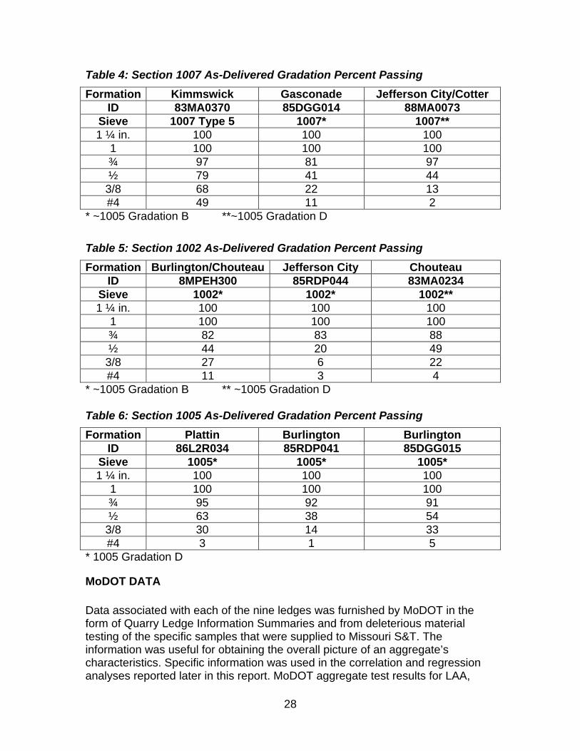
28

Table 4: Section 1007 As-Delivered Gradation Percent Passing

Formation Kimmswick Gasconade Jefferson City/Cotter ID 83MA0370 85DGG014 88MA0073

Sieve 1007 Type 5 1007* 1007** 1 ¼ in. 100 100 100

1 100 100 100 ¾ 97 81 97 ½ 79 41 44 3/8 68 22 13 #4 49 11 2

* ~1005 Gradation B **~1005 Gradation D

Table 5: Section 1002 As-Delivered Gradation Percent Passing

Formation Burlington/Chouteau Jefferson City Chouteau ID 8MPEH300 85RDP044 83MA0234

Sieve 1002* 1002* 1002** 1 ¼ in. 100 100 100

1 100 100 100 ¾ 82 83 88 ½ 44 20 49 3/8 27 6 22 #4 11 3 4

* ~1005 Gradation B ** ~1005 Gradation D Table 6: Section 1005 As-Delivered Gradation Percent Passing

Formation Plattin Burlington Burlington ID 86L2R034 85RDP041 85DGG015

Sieve 1005* 1005* 1005* 1 ¼ in. 100 100 100

1 100 100 100 ¾ 95 92 91 ½ 63 38 54 3/8 30 14 33 #4 3 1 5

* 1005 Gradation D

MoDOT DATA Data associated with each of the nine ledges was furnished by MoDOT in the form of Quarry Ledge Information Summaries and from deleterious material testing of the specific samples that were supplied to Missouri S&T. The information was useful for obtaining the overall picture of an aggregate’s characteristics. Specific information was used in the correlation and regression analyses reported later in this report. MoDOT aggregate test results for LAA,

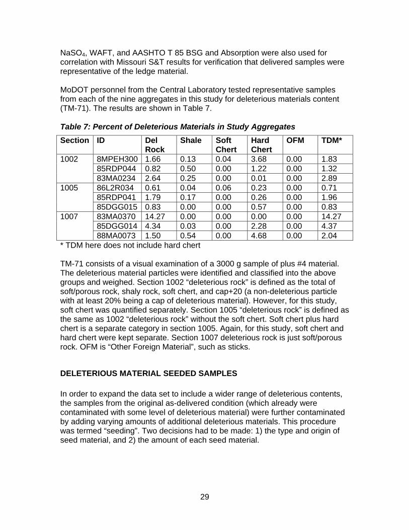
29

NaSO4, WAFT, and AASHTO T 85 BSG and Absorption were also used for correlation with Missouri S&T results for verification that delivered samples were representative of the ledge material. MoDOT personnel from the Central Laboratory tested representative samples from each of the nine aggregates in this study for deleterious materials content (TM-71). The results are shown in Table 7. Table 7: Percent of Deleterious Materials in Study Aggregates

Section ID Del Shale Soft Hard OFM TDM* Rock Chert Chert

1002 8MPEH300 1.66 0.13 0.04 3.68 0.00 1.83 85RDP044 0.82 0.50 0.00 1.22 0.00 1.32 83MA0234 2.64 0.25 0.00 0.01 0.00 2.89

1005 86L2R034 0.61 0.04 0.06 0.23 0.00 0.71 85RDP041 1.79 0.17 0.00 0.26 0.00 1.96 85DGG015 0.83 0.00 0.00 0.57 0.00 0.83

1007 83MA0370 14.27 0.00 0.00 0.00 0.00 14.27 85DGG014 4.34 0.03 0.00 2.28 0.00 4.37 88MA0073 1.50 0.54 0.00 4.68 0.00 2.04

* TDM here does not include hard chert TM-71 consists of a visual examination of a 3000 g sample of plus #4 material. The deleterious material particles were identified and classified into the above groups and weighed. Section 1002 “deleterious rock” is defined as the total of soft/porous rock, shaly rock, soft chert, and cap+20 (a non-deleterious particle with at least 20% being a cap of deleterious material). However, for this study, soft chert was quantified separately. Section 1005 “deleterious rock” is defined as the same as 1002 “deleterious rock” without the soft chert. Soft chert plus hard chert is a separate category in section 1005. Again, for this study, soft chert and hard chert were kept separate. Section 1007 deleterious rock is just soft/porous rock. OFM is “Other Foreign Material”, such as sticks.

DELETERIOUS MATERIAL SEEDED SAMPLES

In order to expand the data set to include a wider range of deleterious contents, the samples from the original as-delivered condition (which already were contaminated with some level of deleterious material) were further contaminated by adding varying amounts of additional deleterious materials. This procedure was termed “seeding”. Two decisions had to be made: 1) the type and origin of seed material, and 2) the amount of each seed material.

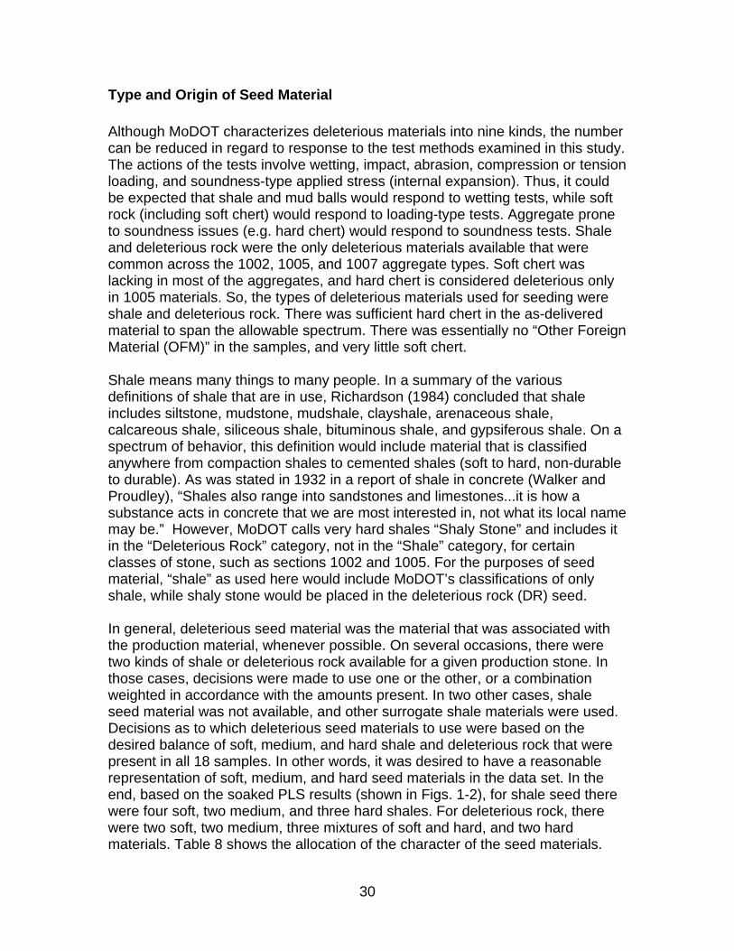
30

Type and Origin of Seed Material

Although MoDOT characterizes deleterious materials into nine kinds, the number can be reduced in regard to response to the test methods examined in this study. The actions of the tests involve wetting, impact, abrasion, compression or tension loading, and soundness-type applied stress (internal expansion). Thus, it could be expected that shale and mud balls would respond to wetting tests, while soft rock (including soft chert) would respond to loading-type tests. Aggregate prone to soundness issues (e.g. hard chert) would respond to soundness tests. Shale and deleterious rock were the only deleterious materials available that were common across the 1002, 1005, and 1007 aggregate types. Soft chert was lacking in most of the aggregates, and hard chert is considered deleterious only in 1005 materials. So, the types of deleterious materials used for seeding were shale and deleterious rock. There was sufficient hard chert in the as-delivered material to span the allowable spectrum. There was essentially no “Other Foreign Material (OFM)” in the samples, and very little soft chert. Shale means many things to many people. In a summary of the various definitions of shale that are in use, Richardson (1984) concluded that shale includes siltstone, mudstone, mudshale, clayshale, arenaceous shale, calcareous shale, siliceous shale, bituminous shale, and gypsiferous shale. On a spectrum of behavior, this definition would include material that is classified anywhere from compaction shales to cemented shales (soft to hard, non-durable to durable). As was stated in 1932 in a report of shale in concrete (Walker and Proudley), “Shales also range into sandstones and limestones...it is how a substance acts in concrete that we are most interested in, not what its local name may be.” However, MoDOT calls very hard shales “Shaly Stone” and includes it in the “Deleterious Rock” category, not in the “Shale” category, for certain classes of stone, such as sections 1002 and 1005. For the purposes of seed material, “shale” as used here would include MoDOT’s classifications of only shale, while shaly stone would be placed in the deleterious rock (DR) seed. In general, deleterious seed material was the material that was associated with the production material, whenever possible. On several occasions, there were two kinds of shale or deleterious rock available for a given production stone. In those cases, decisions were made to use one or the other, or a combination weighted in accordance with the amounts present. In two other cases, shale seed material was not available, and other surrogate shale materials were used. Decisions as to which deleterious seed materials to use were based on the desired balance of soft, medium, and hard shale and deleterious rock that were present in all 18 samples. In other words, it was desired to have a reasonable representation of soft, medium, and hard seed materials in the data set. In the end, based on the soaked PLS results (shown in Figs. 1-2), for shale seed there were four soft, two medium, and three hard shales. For deleterious rock, there were two soft, two medium, three mixtures of soft and hard, and two hard materials. Table 8 shows the allocation of the character of the seed materials.

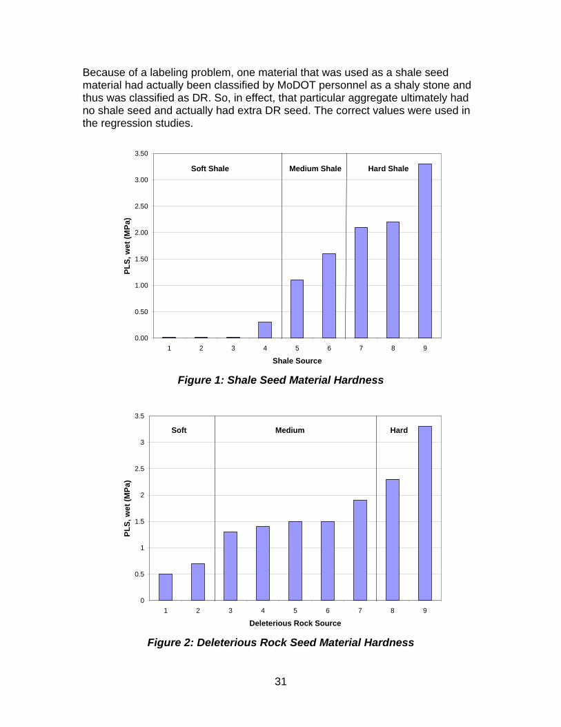
31

Because of a labeling problem, one material that was used as a shale seed material had actually been classified by MoDOT personnel as a shaly stone and thus was classified as DR. So, in effect, that particular aggregate ultimately had no shale seed and actually had extra DR seed. The correct values were used in the regression studies.

0.00

0.50

1.00

1.50

2.00

2.50

3.00

3.50

1 2 3 4 5 6 7 8 9

Shale Source

PL

S, w

et

(MP

a)

Soft Shale Hard ShaleMedium Shale

Figure 1: Shale Seed Material Hardness

0

0.5

1

1.5

2

2.5

3

3.5

1 2 3 4 5 6 7 8 9

Deleterious Rock Source

PL

S, w

et

(MP

a)

Soft Medium Hard

Figure 2: Deleterious Rock Seed Material Hardness

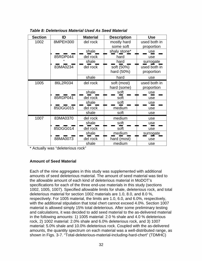
32

Table 8: Deleterious Material Used As Seed Material

Section ID Material Description Use 1002 8MPEH300 del rock mostly hard used both in

some soft proportion shale shaly stone* use

85RDP044 del rock hard use “ shale hard surrogate

83MA0234 del rock soft (50%) used both in

hard (50%) proportion

shale hard use

1005 86L2R034 del rock soft (most) used both in hard (some) proportion

shale soft use

85RDP041 del rock soft use shale soft use

85DGG015 del rock medium use shale soft use

1007 83MA0370 del rock medium use shale soft use

85DGG014

88MA0073

del rock soft use shale

del rock

medium

hard (most)

surrogate

use shale medium use

* Actually was “deleterious rock”

Amount of Seed Material

Each of the nine aggregates in this study was supplemented with additional amounts of seed deleterious material. The amount of seed material was tied to the allowable amount of each kind of deleterious material in MoDOT’s specifications for each of the three end-use materials in this study (sections 1002, 1005, 1007). Specified allowable limits for shale, deleterious rock, and total deleterious material for section 1002 materials are 1.0, 8.0, and 8.0 %, respectively. For 1005 material, the limits are 1.0, 6.0, and 6.0%, respectively, with the additional stipulation that total chert cannot exceed 4.0%. Section 1007 material is allowed simply 15% total deleterious. After some preliminary testing and calculations, it was decided to add seed material to the as-delivered material in the following amounts: 1) 1005 material: 2.0 % shale and 4.0 % deleterious rock, 2) 1002 material: 2.0% shale and 6.0% deleterious rock, and 3) 1007 material: 5.0% shale and 10.0% deleterious rock. Coupled with the as-delivered amounts, the quantity spectrum on each material was a well-distributed range, as shown in Figs. 3-7. “Total-deleterious-material-including-hard-chert” (TDMHC)

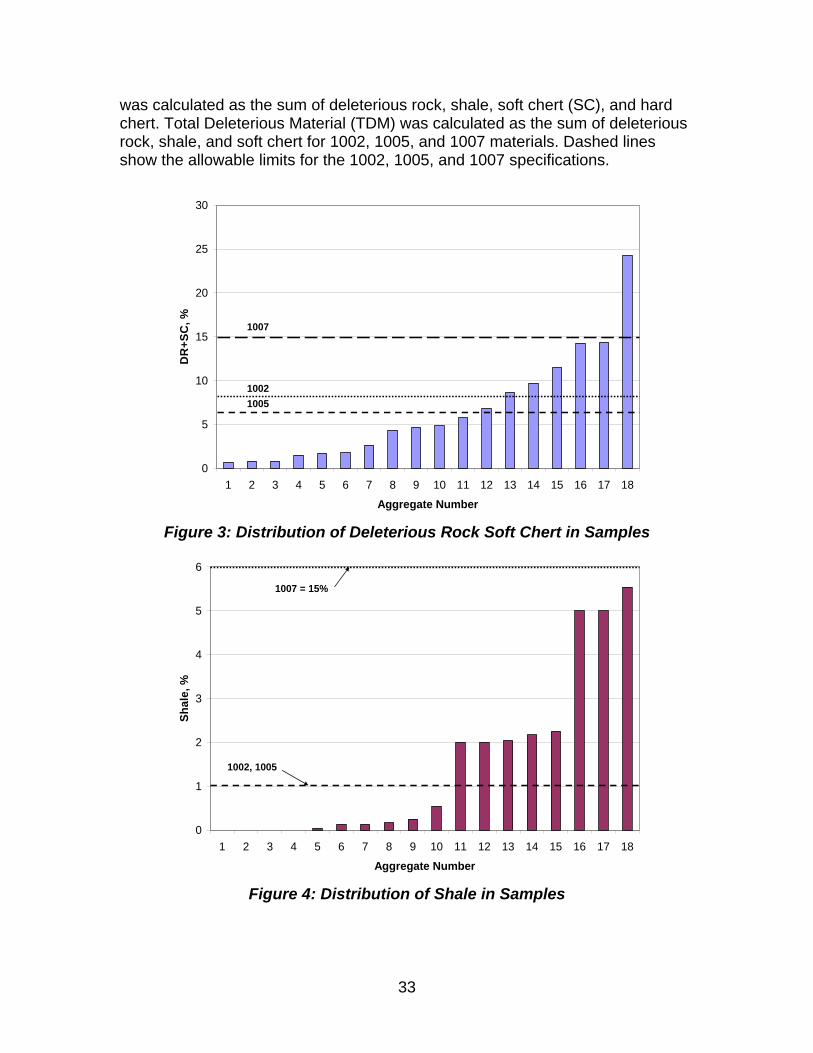
33

was calculated as the sum of deleterious rock, shale, soft chert (SC), and hard chert. Total Deleterious Material (TDM) was calculated as the sum of deleterious rock, shale, and soft chert for 1002, 1005, and 1007 materials. Dashed lines show the allowable limits for the 1002, 1005, and 1007 specifications.

0

5

10

15

20

25

30

1 2 3 4 5 6 7 8 9 10 11 12 13 14 15 16 17 18

Aggregate Number

DR

+S

C, %

1005

1002

1007

Figure 3: Distribution of Deleterious Rock Soft Chert in Samples

0

1

2

3

4

5

6

1 2 3 4 5 6 7 8 9 10 11 12 13 14 15 16 17 18

Aggregate Number

Sh

ale,

%

1007 = 15%

1002, 1005

Figure 4: Distribution of Shale in Samples

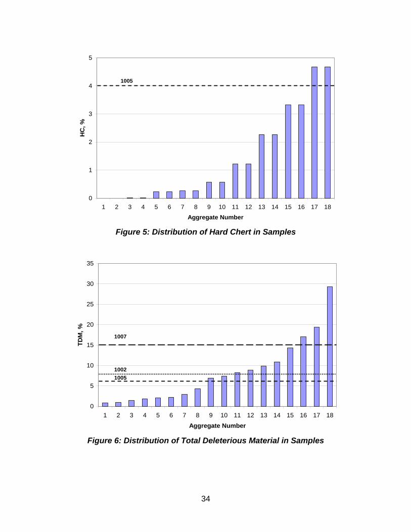
34

0

1

2

3

4

5

1 2 3 4 5 6 7 8 9 10 11 12 13 14 15 16 17 18

Aggregate Number

HC

, %

1005

Figure 5: Distribution of Hard Chert in Samples

0

5

10

15

20

25

30

35

1 2 3 4 5 6 7 8 9 10 11 12 13 14 15 16 17 18

Aggregate Number

TD

M, %

1007

1002

1005

Figure 6: Distribution of Total Deleterious Material in Samples

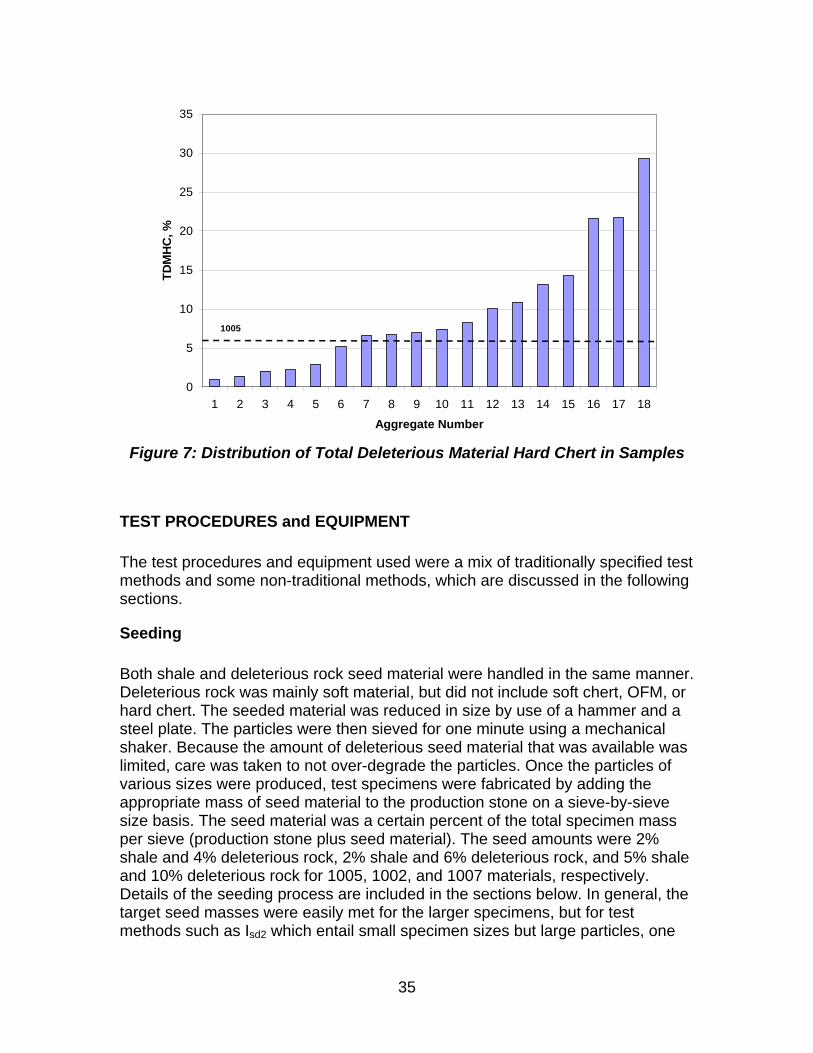
35

0

5

10

15

20

25

30

35

1 2 3 4 5 6 7 8 9 10 11 12 13 14 15 16 17 18

Aggregate Number

TD

MH

C, %

1005

Figure 7: Distribution of Total Deleterious Material Hard Chert in Samples

TEST PROCEDURES and EQUIPMENT

The test procedures and equipment used were a mix of traditionally specified test methods and some non-traditional methods, which are discussed in the following sections.

Seeding

Both shale and deleterious rock seed material were handled in the same manner. Deleterious rock was mainly soft material, but did not include soft chert, OFM, or hard chert. The seeded material was reduced in size by use of a hammer and a steel plate. The particles were then sieved for one minute using a mechanical shaker. Because the amount of deleterious seed material that was available was limited, care was taken to not over-degrade the particles. Once the particles of various sizes were produced, test specimens were fabricated by adding the appropriate mass of seed material to the production stone on a sieve-by-sieve size basis. The seed material was a certain percent of the total specimen mass per sieve (production stone plus seed material). The seed amounts were 2% shale and 4% deleterious rock, 2% shale and 6% deleterious rock, and 5% shale and 10% deleterious rock for 1005, 1002, and 1007 materials, respectively. Details of the seeding process are included in the sections below. In general, the target seed masses were easily met for the larger specimens, but for test methods such as Isd2 which entail small specimen sizes but large particles, one

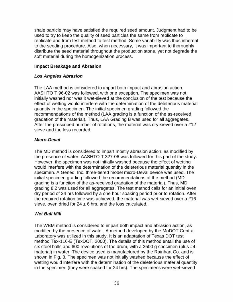
36

shale particle may have satisfied the required seed amount. Judgment had to be used to try to keep the quality of seed particles the same from replicate to replicate and from test method to test method. Some variability was thus inherent to the seeding procedure. Also, when necessary, it was important to thoroughly distribute the seed material throughout the production stone, yet not degrade the soft material during the homogenization process.

Impact Breakage and Abrasion


The LAA method is considered to impart both impact and abrasion action. AASHTO T 96-02 was followed, with one exception. The specimen was not initially washed nor was it wet-sieved at the conclusion of the test because the effect of wetting would interfere with the determination of the deleterious material quantity in the specimen. The initial specimen grading followed the recommendations of the method (LAA grading is a function of the as-received gradation of the material). Thus, LAA Grading B was used for all aggregates. After the prescribed number of rotations, the material was dry-sieved over a #12 sieve and the loss recorded.

Micro-Deval

The MD method is considered to impart mostly abrasion action, as modified by the presence of water. AASHTO T 327-06 was followed for this part of the study. However, the specimen was not initially washed because the effect of wetting would interfere with the determination of the deleterious material quantity in the specimen. A Geneq, Inc. three-tiered model micro-Deval device was used. The initial specimen grading followed the recommendations of the method (MD grading is a function of the as-received gradation of the material). Thus, MD grading 8.2 was used for all aggregates. The test method calls for an initial oven dry period of 24 hrs followed by a one hour soaking period prior to rotation. After the required rotation time was achieved, the material was wet-sieved over a #16 sieve, oven dried for 24 ± 6 hrs, and the loss calculated.

Wet Ball Mill

The WBM method is considered to impart both impact and abrasion action, as modified by the presence of water. A method developed by the MoDOT Central Laboratory was utilized in this study. It is an adaptation of Texas DOT test method Tex-116-E (TexDOT, 2000). The details of this method entail the use of six steel balls and 600 revolutions of the drum, with a 2500 g specimen (plus #4 material) in water. The device used is manufactured by the Rainhart Co. and is shown in Fig. 8. The specimen was not initially washed because the effect of wetting would interfere with the determination of the deleterious material quantity in the specimen (they were soaked for 24 hrs). The specimens were wet-sieved

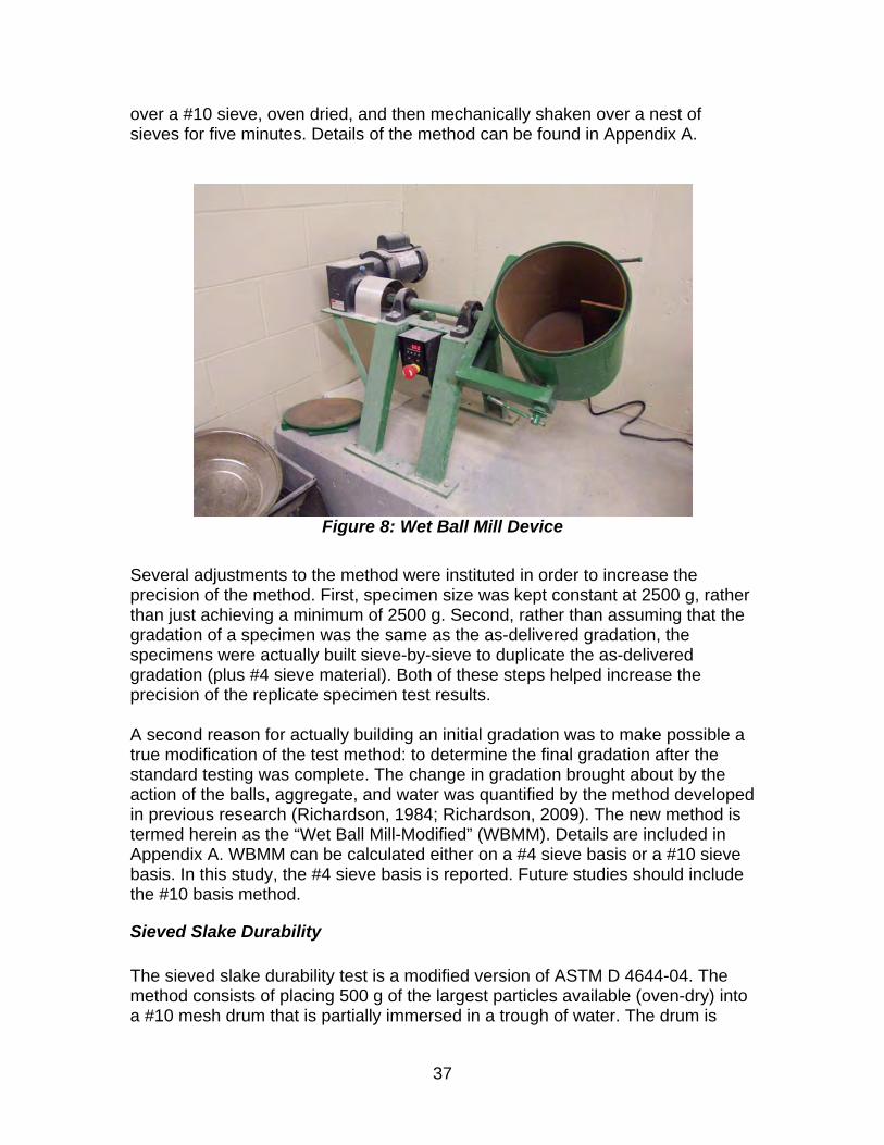
37

over a #10 sieve, oven dried, and then mechanically shaken over a nest of sieves for five minutes. Details of the method can be found in Appendix A.

Figure 8: Wet Ball Mill Device

Several adjustments to the method were instituted in order to increase the precision of the method. First, specimen size was kept constant at 2500 g, rather than just achieving a minimum of 2500 g. Second, rather than assuming that the gradation of a specimen was the same as the as-delivered gradation, the specimens were actually built sieve-by-sieve to duplicate the as-delivered gradation (plus #4 sieve material). Both of these steps helped increase the precision of the replicate specimen test results. A second reason for actually building an initial gradation was to make possible a true modification of the test method: to determine the final gradation after the standard testing was complete. The change in gradation brought about by the action of the balls, aggregate, and water was quantified by the method developed in previous research (Richardson, 1984; Richardson, 2009). The new method is termed herein as the “Wet Ball Mill-Modified” (WBMM). Details are included in Appendix A. WBMM can be calculated either on a #4 sieve basis or a #10 sieve basis. In this study, the #4 sieve basis is reported. Future studies should include the #10 basis method.

Sieved Slake Durability The sieved slake durability test is a modified version of ASTM D 4644-04. The method consists of placing 500 g of the largest particles available (oven-dry) into a #10 mesh drum that is partially immersed in a trough of water. The drum is

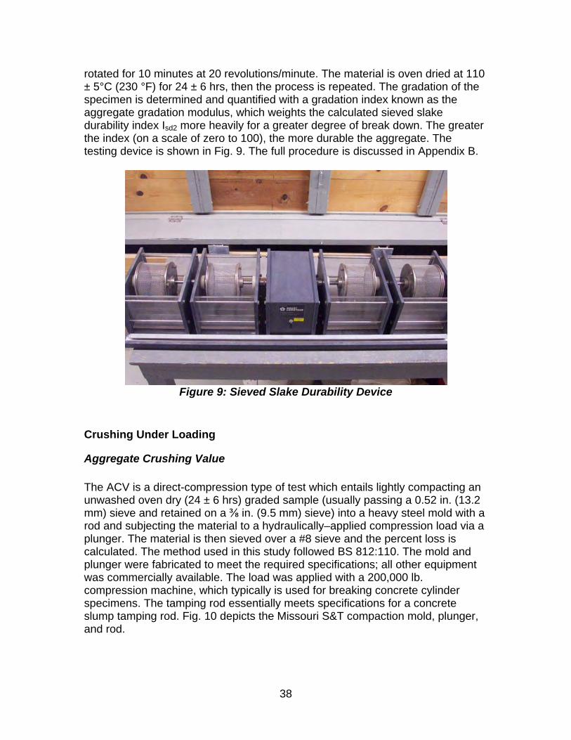
38

rotated for 10 minutes at 20 revolutions/minute. The material is oven dried at 110 ± 5°C (230 °F) for 24 ± 6 hrs, then the process is repeated. The gradation of the specimen is determined and quantified with a gradation index known as the aggregate gradation modulus, which weights the calculated sieved slake durability index Isd2 more heavily for a greater degree of break down. The greater the index (on a scale of zero to 100), the more durable the aggregate. The testing device is shown in Fig. 9. The full procedure is discussed in Appendix B.

Figure 9: Sieved Slake Durability Device

Crushing Under Loading


The ACV is a direct-compression type of test which entails lightly compacting an unwashed oven dry (24 ± 6 hrs) graded sample (usually passing a 0.52 in. (13.2 mm) sieve and retained on a ⅜ in. (9.5 mm) sieve) into a heavy steel mold with a rod and subjecting the material to a hydraulically–applied compression load via a plunger. The material is then sieved over a #8 sieve and the percent loss is calculated. The method used in this study followed BS 812:110. The mold and plunger were fabricated to meet the required specifications; all other equipment was commercially available. The load was applied with a 200,000 lb. compression machine, which typically is used for breaking concrete cylinder specimens. The tamping rod essentially meets specifications for a concrete slump tamping rod. Fig. 10 depicts the Missouri S&T compaction mold, plunger, and rod.

39

Figure 10: Missouri S&T ACV Mold, Rod, and Plunger

The material is gently compacted into the mold by dropping the tamping rod 25 times from a height of one in. per each of three layers. The compression load is then applied over a period of 10 minutes, increasing constantly until an ultimate value of 89,924 lbs. is reached. The dry material is then mechanically shaken over a #8 (2.36 mm) sieve and the loss is calculated as the ACV. The full procedure is reported in Appendix C.

Point Load Strength

The PLS method is basically a tensile-failure type test. ASTM D 5731-07 was followed with several deviations. The method calls for testing 20 pieces of oven-dried (24 ± 6 hrs) aggregate at least 30 mm in size. Each piece is placed between the testing machine’s platens (points) and loaded to failure. The final load and the distance between the points at failure are recorded. The point load strength is mathematically corrected to a standard 50 mm size. Because the purpose of this test in the context of this study is to identify small percentages of soft and water-sensitive materials, the standard procedure of discarding the two greatest and two smallest values was omitted. Any of the 20 pieces that disintegrated prior to testing in the load frame were assigned a strength of zero and were included in the data set. The point load device is shown in Fig. 11.

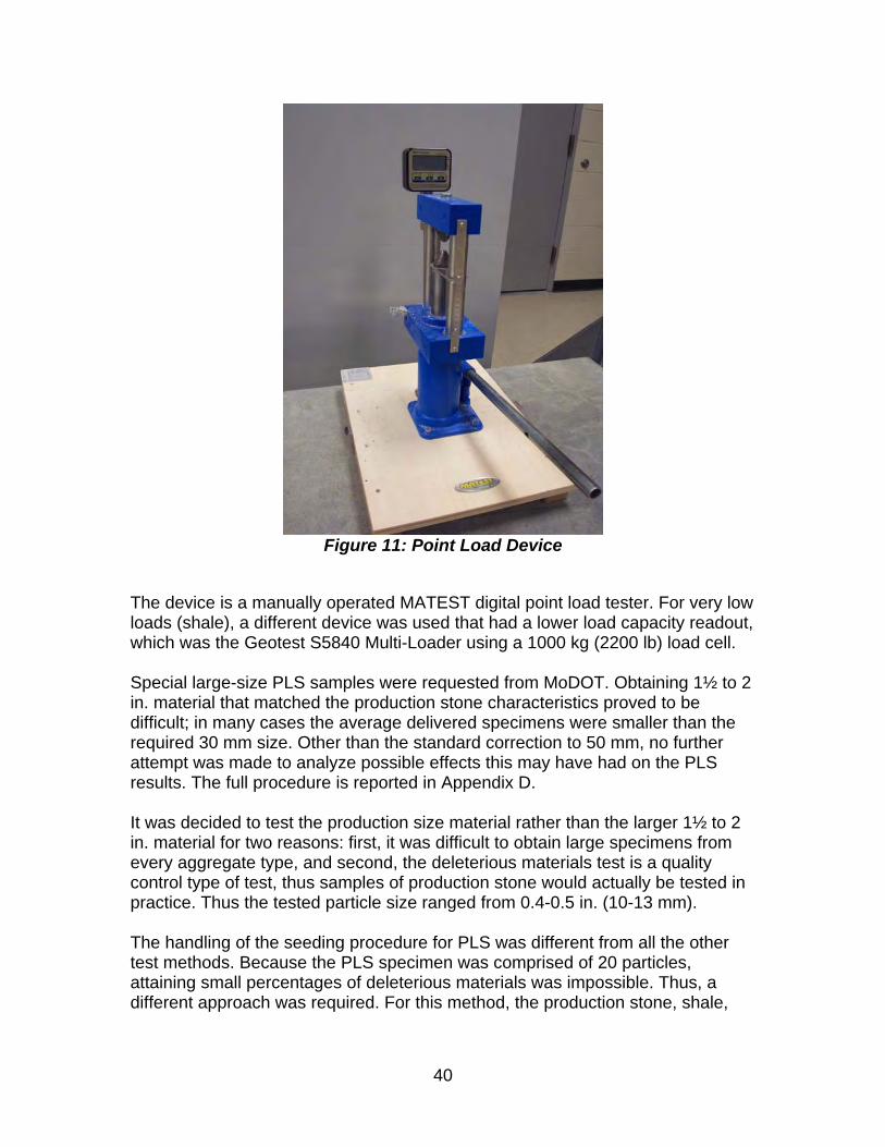
40

Figure 11: Point Load Device

The device is a manually operated MATEST digital point load tester. For very low loads (shale), a different device was used that had a lower load capacity readout, which was the Geotest S5840 Multi-Loader using a 1000 kg (2200 lb) load cell. Special large-size PLS samples were requested from MoDOT. Obtaining 1½ to 2 in. material that matched the production stone characteristics proved to be difficult; in many cases the average delivered specimens were smaller than the required 30 mm size. Other than the standard correction to 50 mm, no further attempt was made to analyze possible effects this may have had on the PLS results. The full procedure is reported in Appendix D. It was decided to test the production size material rather than the larger 1½ to 2 in. material for two reasons: first, it was difficult to obtain large specimens from every aggregate type, and second, the deleterious materials test is a quality control type of test, thus samples of production stone would actually be tested in practice. Thus the tested particle size ranged from 0.4-0.5 in. (10-13 mm). The handling of the seeding procedure for PLS was different from all the other test methods. Because the PLS specimen was comprised of 20 particles, attaining small percentages of deleterious materials was impossible. Thus, a different approach was required. For this method, the production stone, shale,

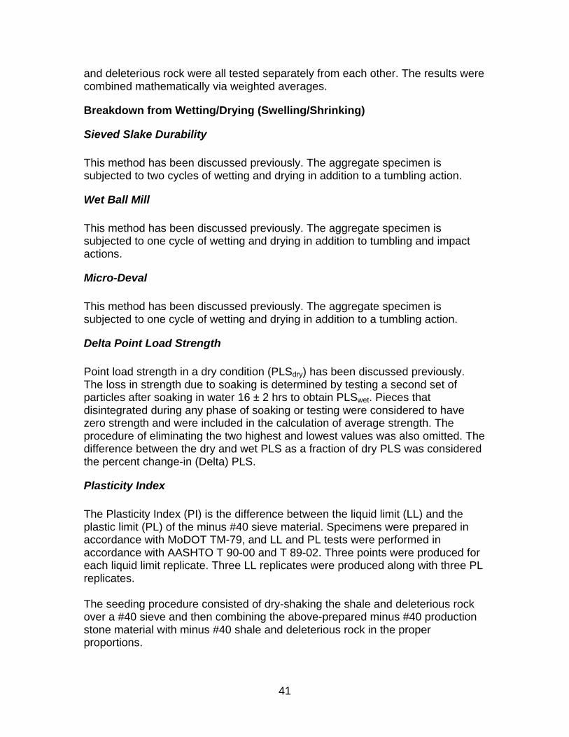
41

and deleterious rock were all tested separately from each other. The results were combined mathematically via weighted averages.

Breakdown from Wetting/Drying (Swelling/Shrinking)

Sieved Slake Durability This method has been discussed previously. The aggregate specimen is subjected to two cycles of wetting and drying in addition to a tumbling action.

Wet Ball Mill This method has been discussed previously. The aggregate specimen is subjected to one cycle of wetting and drying in addition to tumbling and impact actions.

Micro-Deval This method has been discussed previously. The aggregate specimen is subjected to one cycle of wetting and drying in addition to a tumbling action.

Delta Point Load Strength

Point load strength in a dry condition (PLSdry) has been discussed previously. The loss in strength due to soaking is determined by testing a second set of particles after soaking in water 16 ± 2 hrs to obtain PLSwet. Pieces that disintegrated during any phase of soaking or testing were considered to have zero strength and were included in the calculation of average strength. The procedure of eliminating the two highest and lowest values was also omitted. The difference between the dry and wet PLS as a fraction of dry PLS was considered the percent change-in (Delta) PLS.

Plasticity Index The Plasticity Index (PI) is the difference between the liquid limit (LL) and the plastic limit (PL) of the minus #40 sieve material. Specimens were prepared in accordance with MoDOT TM-79, and LL and PL tests were performed in accordance with AASHTO T 90-00 and T 89-02. Three points were produced for each liquid limit replicate. Three LL replicates were produced along with three PL replicates. The seeding procedure consisted of dry-shaking the shale and deleterious rock over a #40 sieve and then combining the above-prepared minus #40 production stone material with minus #40 shale and deleterious rock in the proper proportions.

42

Methylene Blue The Methylene Blue Value is a measure of the presence of certain clay minerals. The test method followed AASHTO T 330-07. Fine production stone material (minus #40 sieve) from the preparation of the PI test material was dry sieved over a #200 sieve, as was the shale and deleterious rock seed material. The three materials were then blended in the proper proportions. A slurry was made with the material, then titrated with methylene blue solution. The full procedure is reported in Appendix E.

Sand Equivalent

Sand Equivalent testing was performed in accordance with AASHTO T 176-02 (Method 1 Air Dry), utilizing the SE mechanical shaker device. The specimen was prepared by separating the as-delivered material over a #4 sieve. The plus #4 material was cleaned by rubbing the material between the hands, as per ASTM D 2419-02 (ASTM, 2002); the minus #4 material produced in that manner was then added to the material that had already passed the #4 sieve. Then, the combined minus #4 material was reduced by riffle splitting down to a specimen size that would fill a moisture-type tin. Special care was exercised when adding the seed material to the production stone so that the seed material did not segregate prior to and during the addition process: 150 g specimens were built according to the seed percentages, then homogenized prior to placing in the specimen tin.

Expansion/Contraction from Freezing/Thawing

Damage from freezing/thawing has been linked to four contributors: 1) aggregate pore characteristics, 2) aggregate pore length, 3) mineralogy, and 4) elastic accommodation/strength.

Aggregate Pore Characteristics The following are tests that reflect some aspect of the manner of the aggregate’s ability to take in water and to expel water, disregarding pore length as a variable. Pore size, distribution, and shape are included.

Absorption and Bulk Specific Gravity

AASHTO T 85 BSG is a function of mineralogy (specific gravity of the solids) and porosity. In the past, MoDOT has used a threshold minimum allowable BSG for certain concrete applications. Absorption is a commonly specified property for aggregate quality and has been used by MoDOT as an acceptability criterion. MoDOT personnel performed the tests in accordance with AASHTO T 85. The

43

material tested would be all plus #4 sieve size. The data was obtained from the Quarry Ledge Information Summaries, thus was not specific to the samples tested in this study.

Vacuum Saturated Absorption and Bulk Specific Gravity

The test method in its final form was derived from methods reported in the literature from the Wisconsin DOT (Williamson et al., 2007), the Iowa DOT IM 380 (IDOT, 2004), MCHRP 86-1 (MoDOT, 1993), the maximum theoretical specific gravity of asphalt mixtures (Rice) method AASHTO T 209 (AASHTO, 2005), and AASHTO T 85-02 (AASHTO, 2002). The level of vacuum is essentially the same as in T 209 and Iowa’s method, and slightly greater than the Wisconsin method. The 30 minute vacuum period is the same as Iowa’s and is greater than the other three methods. The specimen is not initially washed because the effect of wetting would interfere with the determination of the deleterious material quantity in the specimen. In essence, ungraded oven-dried material (plus #4 sieve) is subjected to a vacuum of 27.5 ± 2.5 mm mercury absolute pressure for five minutes. Water is introduced under vacuum and eventually covers the aggregate. The specimen is then subjected to agitation for a total of 30 minutes under vacuum (including the initial five minutes). The material is allowed to stand submerged at atmospheric pressure for 24 hrs. At that point, the balance of the procedure follows the T 85 procedure. The full procedure is reported in Appendix F. Fig. 12 depicts the Missouri S&T vacuum saturation station.

Figure 12: Vacuum Saturation Workstation

44

Care was taken to minimize loss of material once the saturated, surface dry (SSD) weight was obtained. However, some loss of material could have occurred prior to weighing during the saturation and soaking steps. Thus the specimen that finally went through the weighing steps may not have contained the full amount of deleterious material.

Water-Alcohol Freeze Thaw

MoDOT’s TM-14 (modified from AASHTO T 103-07, Method B) was followed. The initial specimen gradation was built to a standard gradation, consisting of three fractions: #4 to ⅜ in., ⅜ to ½ in., and ½ to ¾ in. The specimen was not initially washed because the effect of wetting would interfere with the determination of the deleterious material quantity in the specimen. After 16 cycles of freezing and thawing, the specimens were wet-sieved over a #8 sieve; the plus #8 material was oven dried, cooled, and mechanically sieved for five minutes over a #8 sieve. Freezing and thawing cycle durations were initially determined by use of thermocouples placed in specimens undergoing freezing and thawing cycles, with the freezer and thawing tank loaded with the expected number of specimens. It was especially important to get a good distribution of seed material in the test specimens because it was observed that the material in the bottom of the pans experienced a greater amount of degradation due to the water that was left in the pan bottoms during the freeze-thaw cycles.

Sodium Sulfate Soundness The test methodology followed AASHTO T 104-03. However, the specimen was not initially washed because the effect of wetting would interfere with the determination of the deleterious material quantity in the specimen. All aggregate specimens were built to the standard gradation except Ash Grove, which lacked sufficient material for the ¾ - 1 in. size. The soaking cycle lasted 16 hrs. The drying time interval for all samples was established as per the test protocol to be six hours. After the five cycles were concluded, the specimens were flushed, dried, and mechanically shaken for four minutes over the appropriate sieve.

Pore Length

Length of pores was not addressed in this study because all samples had the same nominal maximum size, thus holding pore length essentially constant.

45

Mineralogy

Methylene Blue, Plasticity Index, and Sand Equivalent

These methods have been discussed previously.

Water-Alcohol Freeze-Thaw

This method was previously discussed. Response to freezing and/or ordering of water molecules at cold temperatures has been shown to be related to mineralogy of aggregates, hence the inclusion of the method in the Mineralogy section.

Elastic Accomodation/Strength

The following are tests that reflect some aspect of the manner of the aggregate’s reaction to internal pressure. Reaction can take the forms of being sufficiently strong to resist fracture or elastic enough to accommodate the pressure.

Aggregate Crushing Value, Los Angeles Abrasion, Micro-Deval, Point Load Strength, Wet Ball Mill

These methods were previously discussed.

Water-Alcohol Freeze-Thaw

This method was previously discussed. Elastic and plastic response to the expansion and contraction during freezing and thawing ties this test into the Elastic Accomodation/Strength section of this study.

Asphalt Binder Bond Interference

Methylene Blue, Plasticity Index, and Sand Equivalent These methods were previously discussed.

Water Absorption

Methylene Blue, Plasticity Index, and Sand Equivalent

These methods were previously discussed.

46

Concrete Paste Bond Interference


Clay Lubrication


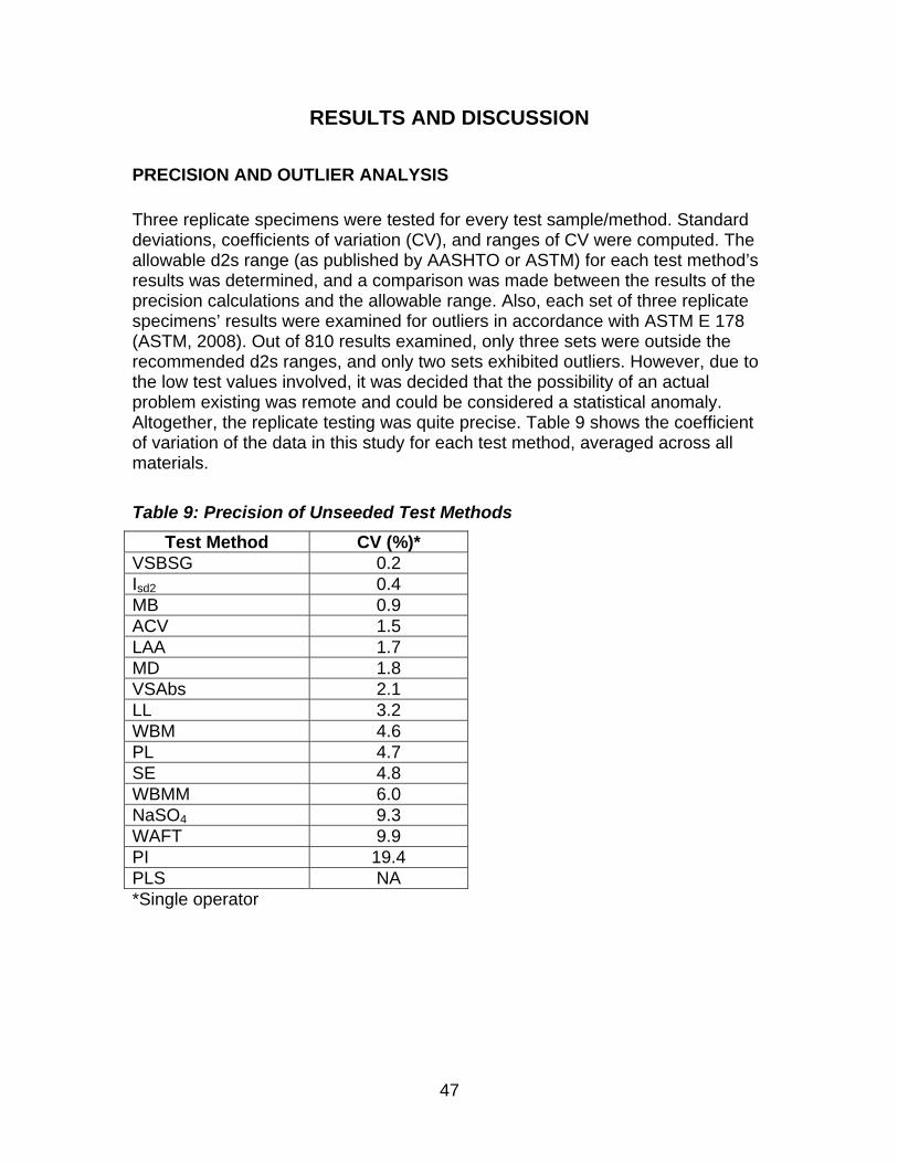
47

RESULTS AND DISCUSSION

PRECISION AND OUTLIER ANALYSIS

Three replicate specimens were tested for every test sample/method. Standard deviations, coefficients of variation (CV), and ranges of CV were computed. The allowable d2s range (as published by AASHTO or ASTM) for each test method’s results was determined, and a comparison was made between the results of the precision calculations and the allowable range. Also, each set of three replicate specimens’ results were examined for outliers in accordance with ASTM E 178 (ASTM, 2008). Out of 810 results examined, only three sets were outside the recommended d2s ranges, and only two sets exhibited outliers. However, due to the low test values involved, it was decided that the possibility of an actual problem existing was remote and could be considered a statistical anomaly. Altogether, the replicate testing was quite precise. Table 9 shows the coefficient of variation of the data in this study for each test method, averaged across all materials.

Table 9: Precision of Unseeded Test Methods

Test Method CV (%)* VSBSG 0.2 Isd2 0.4 MB 0.9 ACV 1.5 LAA 1.7 MD 1.8 VSAbs 2.1 LL 3.2 WBM 4.6 PL 4.7 SE 4.8 WBMM 6.0 NaSO4 9.3 WAFT 9.9 PI 19.4 PLS NA *Single operator

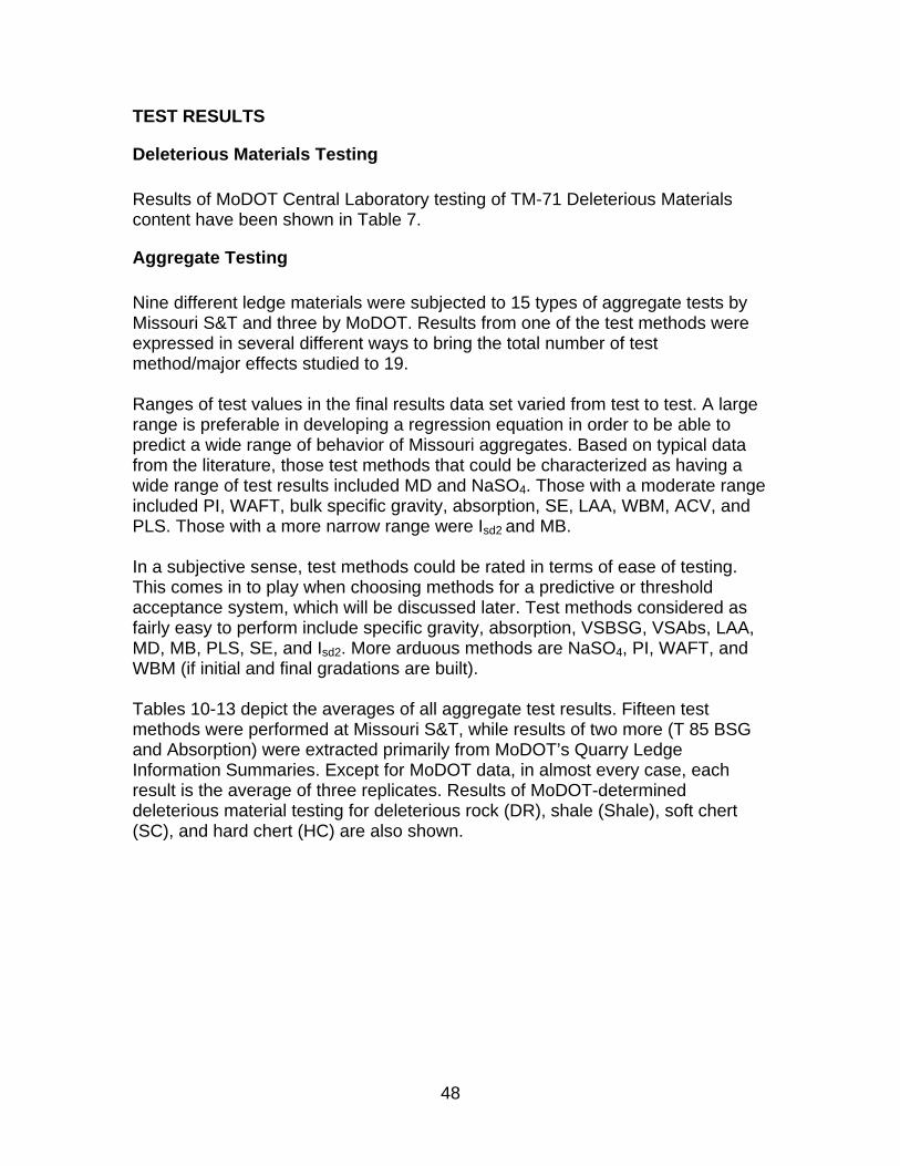
48

TEST RESULTS

Deleterious Materials Testing Results of MoDOT Central Laboratory testing of TM-71 Deleterious Materials content have been shown in Table 7.

Aggregate Testing

Nine different ledge materials were subjected to 15 types of aggregate tests by Missouri S&T and three by MoDOT. Results from one of the test methods were expressed in several different ways to bring the total number of test method/major effects studied to 19. Ranges of test values in the final results data set varied from test to test. A large range is preferable in developing a regression equation in order to be able to predict a wide range of behavior of Missouri aggregates. Based on typical data from the literature, those test methods that could be characterized as having a wide range of test results included MD and NaSO4. Those with a moderate range included PI, WAFT, bulk specific gravity, absorption, SE, LAA, WBM, ACV, and PLS. Those with a more narrow range were Isd2 and MB. In a subjective sense, test methods could be rated in terms of ease of testing. This comes in to play when choosing methods for a predictive or threshold acceptance system, which will be discussed later. Test methods considered as fairly easy to perform include specific gravity, absorption, VSBSG, VSAbs, LAA, MD, MB, PLS, SE, and Isd2. More arduous methods are NaSO4, PI, WAFT, and WBM (if initial and final gradations are built). Tables 10-13 depict the averages of all aggregate test results. Fifteen test methods were performed at Missouri S&T, while results of two more (T 85 BSG and Absorption) were extracted primarily from MoDOT’s Quarry Ledge Information Summaries. Except for MoDOT data, in almost every case, each result is the average of three replicates. Results of MoDOT-determined deleterious material testing for deleterious rock (DR), shale (Shale), soft chert (SC), and hard chert (HC) are also shown.

49

Table 10: Aggregate Test Result Averages

Section ID Formation Condition DR SC HC Shale TDM TDMHC1002 8MPEH300 BurlingtonLS/ChouteauLS unseeded 1.66 0.04 3.68 0.13 1.83 5.511002 8MPEH300 BurlingtonLS/ChouteauLS seeded 9.66 0.04 3.68 0.13 9.83 13.511002 85RDP044 Jeff. City Dolomite unseeded 0.82 0.00 1.22 0.50 1.32 2.541002 85RDP044 Jeff. City Dolomite seeded 6.82 0.00 1.22 2.50 9.32 10.541002 83MA0234 Chouteau LS unseeded 2.64 0.00 0.01 0.25 2.89 2.901002 83MA0234 Chouteau LS seeded 8.64 0.00 0.01 2.25 10.89 10.901005 86L2R034 Plattin LS unseeded 0.61 0.06 0.23 0.04 0.71 0.941005 86L2R034 Plattin LS seeded 4.61 0.06 0.23 2.04 6.71 6.941005 85RDP041 Burlington LS unseeded 1.79 0.00 0.26 0.17 1.96 2.221005 85RDP041 Burlington LS seeded 5.79 0.00 0.26 2.17 7.96 8.221005 85DGG015 Burlington LS unseeded 0.83 0.00 0.57 0.00 0.83 1.401005 85DGG015 Burlington LS seeded 4.83 0.00 0.57 2.00 6.83 7.401007 83MA0370 Kimmswick LS unseeded 14.27 0.00 0.00 0.00 14.27 14.271007 83MA0370 Kimmswick LS seeded 24.27 0.00 0.00 5.00 29.27 29.271007 85DGG014 Gasconade Dolomite unseeded 4.34 0.00 2.28 0.03 4.37 6.651007 85DGG014 Gasconade Dolomite seeded 14.34 0.00 2.28 5.03 19.37 21.651007 88MA0073 Jeff. City-Cotter Dolomite unseeded 1.50 0.00 4.68 0.54 2.04 6.721007 88MA0073 Jeff. City-Cotter Dolomite seeded 11.50 0.00 4.68 5.54 17.04 21.72

Table 11: Aggregate Test Result Averages, continued

Section ID Formation Condition ACV WBM WBMM LAA MB MD1002 8MPEH300 BurlingtonLS/ChouteauLS unseeded 29.8 27.8 30.1 35.7 2.3 27.51002 8MPEH300 BurlingtonLS/ChouteauLS seeded 30.1 29.2 33.1 36.8 2.8 31.21002 85RDP044 Jeff. City Dolomite unseeded 23.3 16.3 23.4 31.4 5.0 17.91002 85RDP044 Jeff. City Dolomite seeded 22.6 18.1 26.2 30.8 5.5 22.21002 83MA0234 Chouteau LS unseeded 29.2 26.6 31.7 35.2 3.3 29.11002 83MA0234 Chouteau LS seeded 29.0 33.1 38.6 37.2 3.0 31.41005 86L2R034 Plattin LS unseeded 26.1 22.5 29.5 26.5 2.0 15.81005 86L2R034 Plattin LS seeded 25.1 26.0 30.6 29.4 3.3 18.11005 85RDP041 Burlington LS unseeded 26.8 19.4 23.3 30.8 3.5 23.71005 85RDP041 Burlington LS seeded 26.0 25.1 30.6 32.0 4.3 27.51005 85DGG015 Burlington LS unseeded 29.7 33.4 38.0 36.6 2.0 19.61005 85DGG015 Burlington LS seeded 28.4 31.3 33.0 34.9 2.0 23.71007 83MA0370 Kimmswick LS unseeded 38.2 53.9 54.2 56.3 4.0 40.51007 83MA0370 Kimmswick LS seeded 39.4 59.7 59.4 58.6 6.1 49.51007 85DGG014 Gasconade Dolomite unseeded 30.6 27.4 33.4 41.2 4.8 25.21007 85DGG014 Gasconade Dolomite seeded 32.1 34.8 39.5 45.9 6.3 29.51007 88MA0073 Jeff. City-Cotter Dolomite unseeded 22.0 17.8 23.6 26.9 4.5 17.21007 88MA0073 Jeff. City-Cotter Dolomite seeded 23.4 23.1 30.0 29.3 5.0 23.3

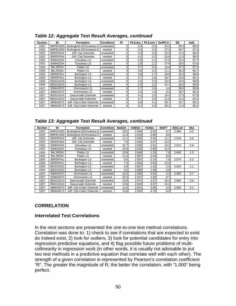
50


Section ID Formation Condition PI PLS,dry PLS,wet DeltPLS SE Isd21002 8MPEH300 BurlingtonLS/ChouteauLS unseeded 2 3.3 2.5 24.2 59.3 98.01002 8MPEH300 BurlingtonLS/ChouteauLS seeded 0 3.3 2.4 27.3 50.7 97.21002 85RDP044 Jeff. City Dolomite unseeded 2 4.3 3.3 23.3 11.0 98.21002 85RDP044 Jeff. City Dolomite seeded 0 4.2 3.2 23.8 11.3 98.31002 83MA0234 Chouteau LS unseeded 3 2.9 2.1 27.6 21.0 97.71002 83MA0234 Chouteau LS seeded 0 2.9 2.1 27.6 19.0 97.61005 86L2R034 Plattin LS unseeded 3 3.7 3.3 10.8 37.3 97.21005 86L2R034 Plattin LS seeded 3 3.6 3.2 11.1 28.3 95.71005 85RDP041 Burlington LS unseeded 3 3.8 2.7 28.9 25.3 98.61005 85RDP041 Burlington LS seeded 2 3.7 2.6 29.7 23.0 95.11005 85DGG015 Burlington LS unseeded 0 3.0 2.3 23.3 42.0 98.81005 85DGG015 Burlington LS seeded 0 2.9 2.2 24.1 40.0 96.81007 83MA0370 Kimmswick LS unseeded 0 1.7 1.6 5.9 39.0 95.91007 83MA0370 Kimmswick LS seeded 0 1.6 1.5 6.3 28.7 90.21007 85DGG014 Gasconade Dolomite unseeded 0 4.1 3.3 19.5 17.3 97.51007 85DGG014 Gasconade Dolomite seeded 0 3.7 2.9 21.6 21.0 93.21007 88MA0073 Jeff. City-Cotter Dolomite unseeded 5 6.8 4.1 39.7 10.7 96.11007 88MA0073 Jeff. City-Cotter Dolomite seeded 3 6.4 3.9 39.1 11.0 96.1


Section ID Formation Condition NaSO4 VSBSG VSAbs WAFT BSG,od Abs1002 8MPEH300 BurlingtonLS/ChouteauLS unseeded 18.0 2.509 3.02 4.7 2.490 3.21002 8MPEH300 BurlingtonLS/ChouteauLS seeded 11.8 2.519 2.95 8.61002 85RDP044 Jeff. City Dolomite unseeded 11.1 2.595 3.20 11.1 2.576 3.01002 85RDP044 Jeff. City Dolomite seeded 7.6 2.560 3.47 13.21002 83MA0234 Chouteau LS unseeded 21.7 2.535 2.61 14.2 2.514 2.61002 83MA0234 Chouteau LS seeded 14.9 2.523 2.83 11.51005 86L2R034 Plattin LS unseeded 13.8 2.640 1.23 7.8 2.640 1.31005 86L2R034 Plattin LS seeded 11.4 2.587 2.03 8.81005 85RDP041 Burlington LS unseeded 9.5 2.597 2.14 7.8 2.574 2.21005 85RDP041 Burlington LS seeded 7.5 2.563 2.50 13.01005 85DGG015 Burlington LS unseeded 5.8 2.607 1.63 2.5 2.624 1.11005 85DGG015 Burlington LS seeded 4.2 2.580 1.99 3.91007 83MA0370 Kimmswick LS unseeded 15.2 2.426 4.53 3.3 2.453 3.71007 83MA0370 Kimmswick LS seeded 20.3 2.427 4.60 9.71007 85DGG014 Gasconade Dolomite unseeded 13.6 2.574 3.37 15.3 2.584 2.61007 85DGG014 Gasconade Dolomite seeded 13.6 2.563 3.37 14.21007 88MA0073 Jeff. City-Cotter Dolomite unseeded 11.6 2.541 3.90 3.0 2.560 3.1

7 88MA0073 Jeff. City-Cotter Dolomite seeded 13.8 2.542 3.79 8.0100

CORRELATION

Interrelated Test Correlations In the next sections are presented the one-to-one test method correlations. Correlation was done to: 1) check to see if correlations that are expected to exist do indeed exist, 2) look for outliers, 3) look for potential candidates for entry into regression predictive equations, and 4) flag possible future problems of multi-collinearity in regression work (in other words, it is usually not advisable to put two test methods in a predictive equation that correlate well with each other). The strength of a given correlation is represented by Pearson’s correlation coefficient “R”. The greater the magnitude of R, the better the correlation, with “1.000” being perfect.

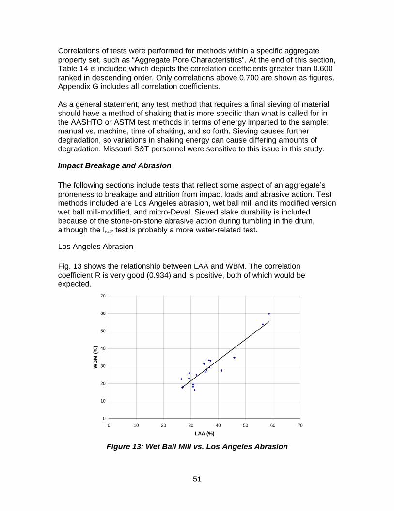
51

Correlations of tests were performed for methods within a specific aggregate property set, such as “Aggregate Pore Characteristics”. At the end of this section, Table 14 is included which depicts the correlation coefficients greater than 0.600 ranked in descending order. Only correlations above 0.700 are shown as figures. Appendix G includes all correlation coefficients. As a general statement, any test method that requires a final sieving of material should have a method of shaking that is more specific than what is called for in the AASHTO or ASTM test methods in terms of energy imparted to the sample: manual vs. machine, time of shaking, and so forth. Sieving causes further degradation, so variations in shaking energy can cause differing amounts of degradation. Missouri S&T personnel were sensitive to this issue in this study.

Impact Breakage and Abrasion The following sections include tests that reflect some aspect of an aggregate’s proneness to breakage and attrition from impact loads and abrasive action. Test methods included are Los Angeles abrasion, wet ball mill and its modified version wet ball mill-modified, and micro-Deval. Sieved slake durability is included because of the stone-on-stone abrasive action during tumbling in the drum, although the Isd2 test is probably a more water-related test.


Fig. 13 shows the relationship between LAA and WBM. The correlation coefficient R is very good (0.934) and is positive, both of which would be expected.

0

10

20

30

40

50

60

70

0 10 20 30 40 50 60 70

LAA (%)

WB

M (

%)

Figure 13: Wet Ball Mill vs. Los Angeles Abrasion

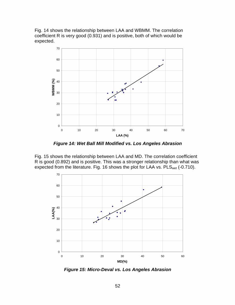
52

Fig. 14 shows the relationship between LAA and WBMM. The correlation coefficient R is very good (0.931) and is positive, both of which would be expected.

0

10

20

30

40

50

60

70

0 10 20 30 40 50 60 70

LAA (%)

WB

MM

(%

)

Figure 14: Wet Ball Mill Modified vs. Los Angeles Abrasion

Fig. 15 shows the relationship between LAA and MD. The correlation coefficient R is good (0.892) and is positive. This was a stronger relationship than what was expected from the literature. Fig. 16 shows the plot for LAA vs. PLSwet (-0.710).

0

10

20

30

40

50

60

70

0 10 20 30 40 50 60

MD(%)

LA

A(%

)

Figure 15: Micro-Deval vs. Los Angeles Abrasion

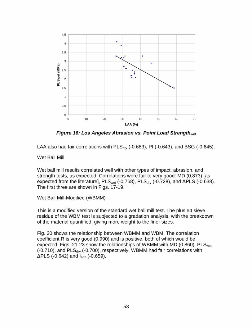
53

0

0.5

1

1.5

2

2.5

3

3.5

4

4.5

0 10 20 30 40 50 60 70

LAA (%)

PL

Sw

et (

MP

a)

Figure 16: Los Angeles Abrasion vs. Point Load Strengthwet

LAA also had fair correlations with PLSdry (-0.683), PI (-0.643), and BSG (-0.645).

Wet Ball Mill

Wet ball mill results correlated well with other types of impact, abrasion, and strength tests, as expected. Correlations were fair to very good: MD (0.873) [as expected from the literature], PLSwet (-0.768), PLSdry (-0.728), and ΔPLS (-0.638). The first three are shown in Figs. 17-19.

Wet Ball Mill-Modified (WBMM)

This is a modified version of the standard wet ball mill test. The plus #4 sieve residue of the WBM test is subjected to a gradation analysis, with the breakdown of the material quantified, giving more weight to the finer sizes. Fig. 20 shows the relationship between WBMM and WBM. The correlation coefficient R is very good (0.990) and is positive, both of which would be expected. Figs. 21-23 show the relationships of WBMM with MD (0.860), PLSwet (-0.710), and PLSdry (-0.700), respectively. WBMM had fair correlations with ΔPLS (-0.642) and Isd2 (-0.659).

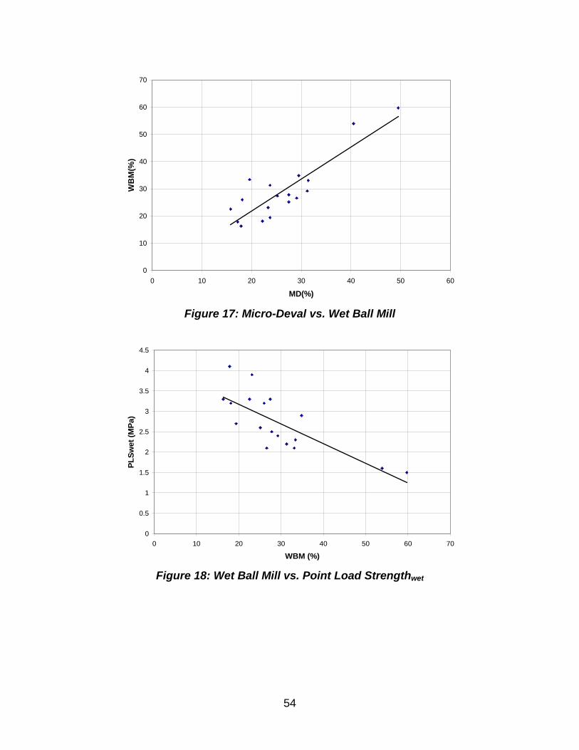
54

0

10

20

30

40

50

60

70

0 10 20 30 40 50 60

MD(%)

WB

M(%

)

Figure 17: Micro-Deval vs. Wet Ball Mill

0

0.5

1

1.5

2

2.5

3

3.5

4

4.5

0 10 20 30 40 50 60 70

WBM (%)

PL

Sw

et (

MP

a)

Figure 18: Wet Ball Mill vs. Point Load Strengthwet

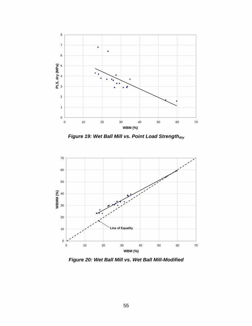
55

0

1

2

3

4

5

6

7

8

0 10 20 30 40 50 60 70

WBM (%)

PL

S, d

ry (

MP

a)

Figure 19: Wet Ball Mill vs. Point Load Strengthdry

0

10

20

30

40

50

60

70

0 10 20 30 40 50 60 70

WBM (%)

WB

MM

(%

)

Line of Equality

Figure 20: Wet Ball Mill vs. Wet Ball Mill-Modified

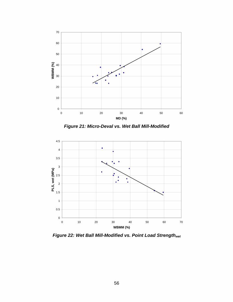
56

0

10

20

30

40

50

60

70

0 10 20 30 40 50 60

MD (%)

WB

MM

(%

)

Figure 21: Micro-Deval vs. Wet Ball Mill-Modified

0

0.5

1

1.5

2

2.5

3

3.5

4

4.5

0 10 20 30 40 50 60 70

WBMM (%)

PL

S, w

et

(MP

a)

Figure 22: Wet Ball Mill-Modified vs. Point Load Strengthwet

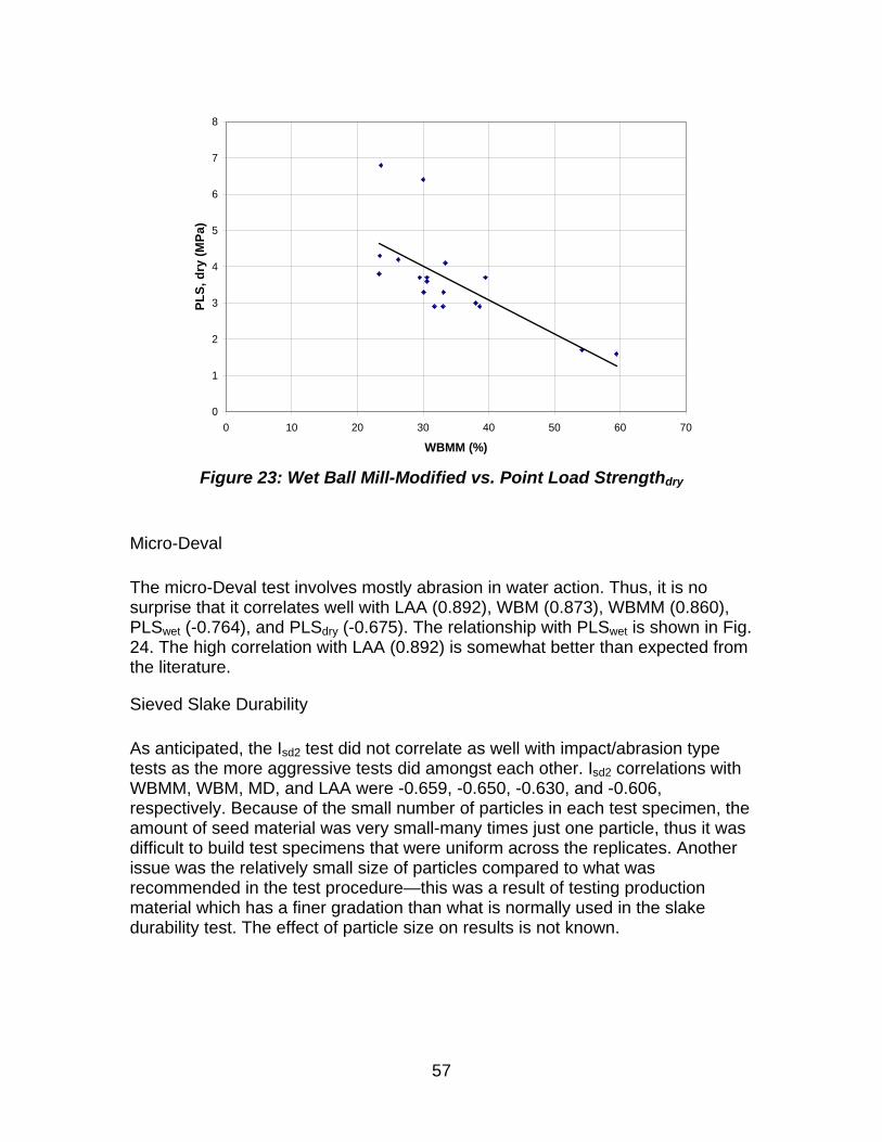
57

0

1

2

3

4

5

6

7

8

0 10 20 30 40 50 60 70

WBMM (%)

PL

S, d

ry (

MP

a)

Figure 23: Wet Ball Mill-Modified vs. Point Load Strengthdry

Micro-Deval

The micro-Deval test involves mostly abrasion in water action. Thus, it is no surprise that it correlates well with LAA (0.892), WBM (0.873), WBMM (0.860), PLSwet (-0.764), and PLSdry (-0.675). The relationship with PLSwet is shown in Fig. 24. The high correlation with LAA (0.892) is somewhat better than expected from the literature.

Sieved Slake Durability

As anticipated, the Isd2 test did not correlate as well with impact/abrasion type tests as the more aggressive tests did amongst each other. Isd2 correlations with WBMM, WBM, MD, and LAA were -0.659, -0.650, -0.630, and -0.606, respectively. Because of the small number of particles in each test specimen, the amount of seed material was very small-many times just one particle, thus it was difficult to build test specimens that were uniform across the replicates. Another issue was the relatively small size of particles compared to what was recommended in the test procedure—this was a result of testing production material which has a finer gradation than what is normally used in the slake durability test. The effect of particle size on results is not known.

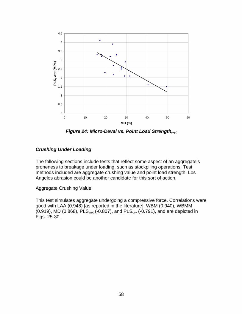
58

0

0.5

1

1.5

2

2.5

3

3.5

4

4.5

0 10 20 30 40 50 60

MD (%)

PL

S, w

et

(MP

a)

Figure 24: Micro-Deval vs. Point Load Strengthwet

Crushing Under Loading

The following sections include tests that reflect some aspect of an aggregate’s proneness to breakage under loading, such as stockpiling operations. Test methods included are aggregate crushing value and point load strength. Los Angeles abrasion could be another candidate for this sort of action.


This test simulates aggregate undergoing a compressive force. Correlations were good with LAA (0.948) [as reported in the literature], WBM (0.940), WBMM (0.919), MD (0.868), PLSwet (-0.807), and PLSdry (-0.791), and are depicted in Figs. 25-30.

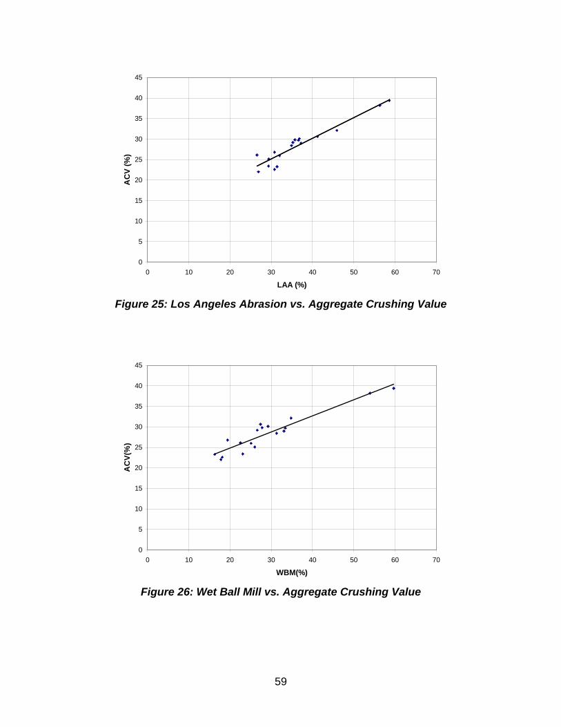
59

0

5

10

15

20

25

30

35

40

45

0 10 20 30 40 50 60 70

LAA (%)

AC

V (

%)

Figure 25: Los Angeles Abrasion vs. Aggregate Crushing Value

0

5

10

15

20

25

30

35

40

45

0 10 20 30 40 50 60 70

WBM(%)

AC

V(%

)

Figure 26: Wet Ball Mill vs. Aggregate Crushing Value

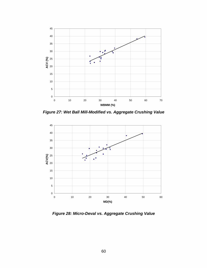
60

0

5

10

15

20

25

30

35

40

45

0 10 20 30 40 50 60 70

WBMM (%)

AC

V (

%)

Figure 27: Wet Ball Mill-Modified vs. Aggregate Crushing Value

0

5

10

15

20

25

30

35

40

45

0 10 20 30 40 50 60

MD(%)

AC

V(%

)

Figure 28: Micro-Deval vs. Aggregate Crushing Value

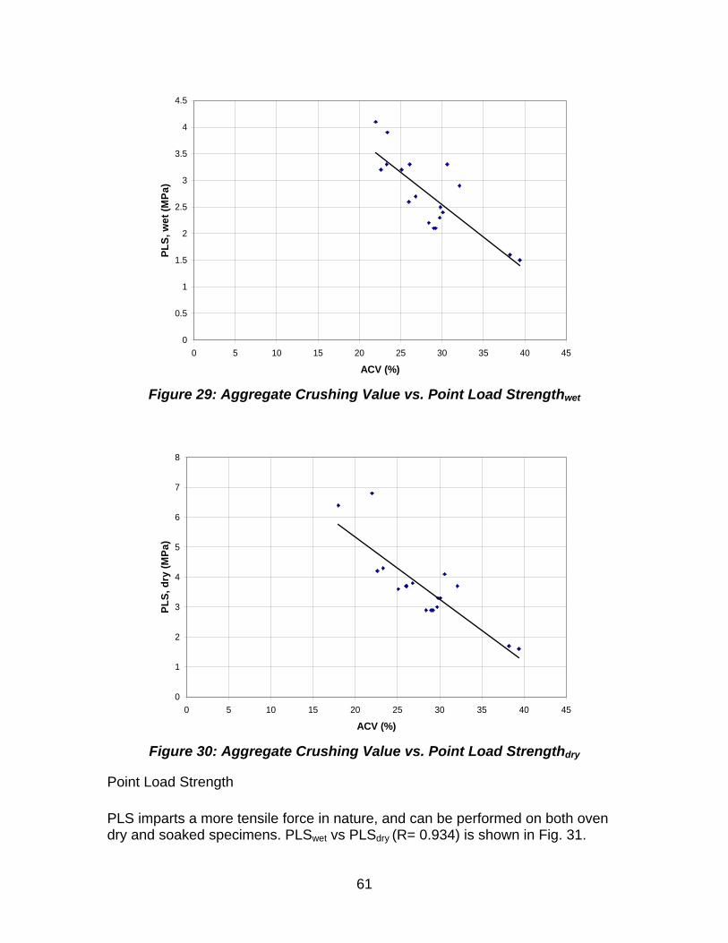
61

0

0.5

1

1.5

2

2.5

3

3.5

4

4.5

0 5 10 15 20 25 30 35 40 45

ACV (%)

PL

S, w

et

(MP

a)

Figure 29: Aggregate Crushing Value vs. Point Load Strengthwet

0

1

2

3

4

5

6

7

8

0 5 10 15 20 25 30 35 40 45

ACV (%)

PL

S, d

ry (

MP

a)

Figure 30: Aggregate Crushing Value vs. Point Load Strengthdry

Point Load Strength

PLS imparts a more tensile force in nature, and can be performed on both oven dry and soaked specimens. PLSwet vs PLSdry (R= 0.934) is shown in Fig. 31.

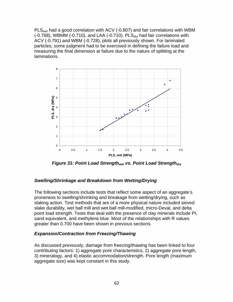
62

PLSwet had a good correlation with ACV (-0.807) and fair correlations with WBM (-0.768), WBMM (-0.710), and LAA (-0.710). PLSdry had fair correlations with ACV (-0.791) and WBM (-0.728), plots all previously shown. For laminated particles, some judgment had to be exercised in defining the failure load and measuring the final dimension at failure due to the nature of splitting at the laminations.

0

1

2

3

4

5

6

7

8

0 0.5 1 1.5 2 2.5 3 3.5 4 4.5

PLS, wet (MPa)

PL

S, d

ry (

MP

a)

Figure 31: Point Load Strengthwet vs. Point Load Strengthdry

Swelling/Shrinkage and Breakdown from Wetting/Drying

The following sections include tests that reflect some aspect of an aggregate’s proneness to swelling/shrinking and breakage from wetting/drying, such as slaking action. Test methods that are of a more physical nature included sieved slake durability, wet ball mill and wet ball mill-modified, micro-Deval, and delta point load strength. Tests that deal with the presence of clay minerals include PI, sand equivalent, and methylene blue. Most of the relationships with R values greater than 0.700 have been shown in previous sections.

Expansion/Contraction from Freezing/Thawing

As discussed previously, damage from freezing/thawing has been linked to four contributing factors: 1) aggregate pore characteristics, 2) aggregate pore length, 3) mineralogy, and 4) elastic accommodation/strength. Pore length (maximum aggregate size) was kept constant in this study.

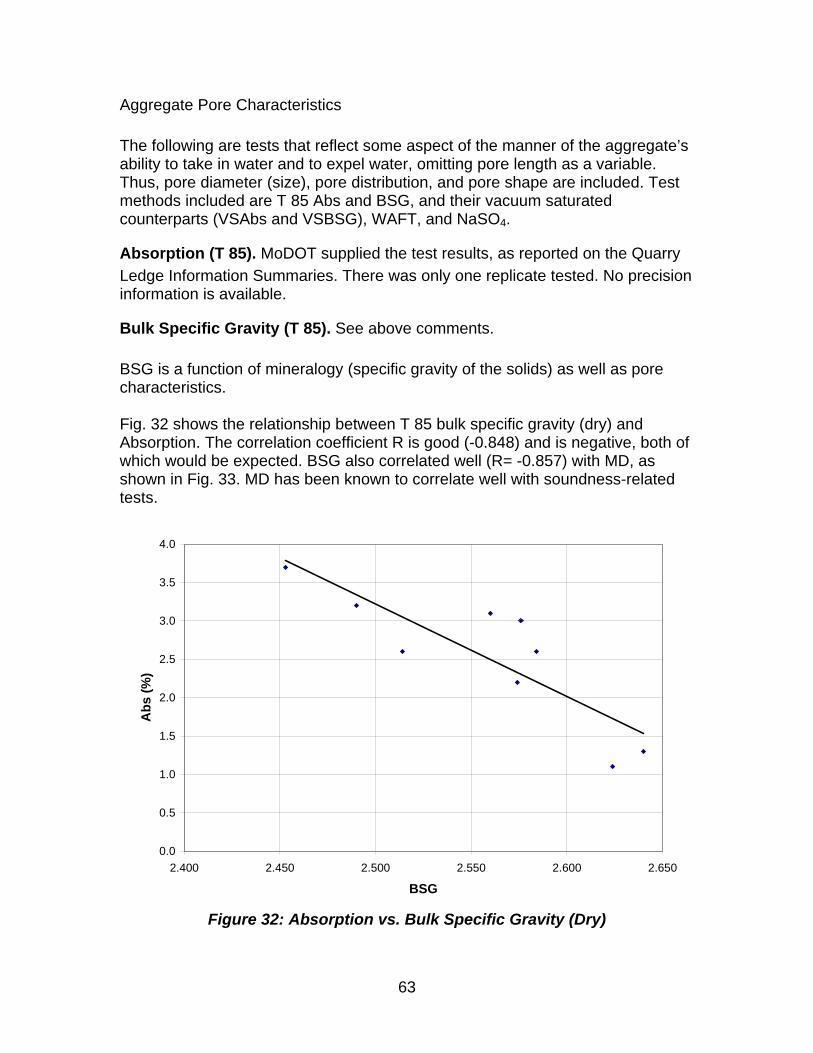
63

Aggregate Pore Characteristics

The following are tests that reflect some aspect of the manner of the aggregate’s ability to take in water and to expel water, omitting pore length as a variable. Thus, pore diameter (size), pore distribution, and pore shape are included. Test methods included are T 85 Abs and BSG, and their vacuum saturated counterparts (VSAbs and VSBSG), WAFT, and NaSO4.

Absorption (T 85). MoDOT supplied the test results, as reported on the Quarry

Ledge Information Summaries. There was only one replicate tested. No precision information is available.

Bulk Specific Gravity (T 85). See above comments.

BSG is a function of mineralogy (specific gravity of the solids) as well as pore characteristics. Fig. 32 shows the relationship between T 85 bulk specific gravity (dry) and Absorption. The correlation coefficient R is good (-0.848) and is negative, both of which would be expected. BSG also correlated well (R= -0.857) with MD, as shown in Fig. 33. MD has been known to correlate well with soundness-related tests.

0.0

0.5

1.0

1.5

2.0

2.5

3.0

3.5

4.0

2.400 2.450 2.500 2.550 2.600 2.650

BSG

Ab

s (%

)

Figure 32: Absorption vs. Bulk Specific Gravity (Dry)

64

0

10

20

30

40

50

60

2.400 2.450 2.500 2.550 2.600 2.650

BSG

MD

(%

)

Figure 33: Bulk Specific Gravity (Dry) vs. Micro-Deval

Vacuum Saturated Absorption. Vacuum saturation should result in more water

being pulled into the aggregate, compared to the standard T 85 24 hr. soak, thus increasing the absorption value. In most cases, this held true. The change in absorption ranged from -0.1 to +0.8%, with an average increase of 0.3%. The comparison is shown below in Fig. 34, with a correlation factor R of 0.926. A paired t-test showed that the two parameters were not statistically different at the 0.05 α level. Other fair-to-good correlations of VSAbs were with T 85 BSG (-0.732), MB (0.730), MD (0.614), and VSBSG (-0.800). The initial soaking period caused some deleterious material degradation and loss of material - the effect of this is not completely known.

Vacuum Saturated Bulk Specific Gravity. Fig. 35 shows the relationship

between VSBSG and VSAbs (R= -0.800) and Fig. 36 shows VSBSG vs. Abs (R= -0.816).

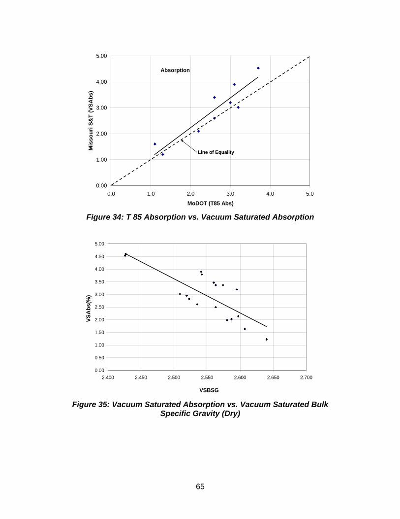
65

0.00

1.00

2.00

3.00

4.00

5.00

0.0 1.0 2.0 3.0 4.0 5.0

MoDOT (T85 Abs)

Mis

sou

ri S

&T

(V

SA

bs)

Line of Equality

Absorption

Figure 34: T 85 Absorption vs. Vacuum Saturated Absorption

0.00

0.50

1.00

1.50

2.00

2.50

3.00

3.50

4.00

4.50

5.00

2.400 2.450 2.500 2.550 2.600 2.650 2.700

VSBSG

VS

Ab

s(%

)

Figure 35: Vacuum Saturated Absorption vs. Vacuum Saturated Bulk

Specific Gravity (Dry)

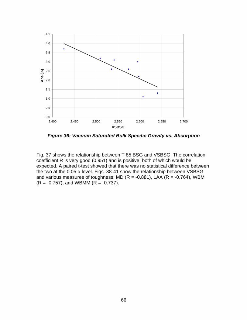
66

0.0

0.5

1.0

1.5

2.0

2.5

3.0

3.5

4.0

4.5

2.400 2.450 2.500 2.550 2.600 2.650 2.700

VSBSG

Ab

s (%

)

Figure 36: Vacuum Saturated Bulk Specific Gravity vs. Absorption

Fig. 37 shows the relationship between T 85 BSG and VSBSG. The correlation coefficient R is very good (0.951) and is positive, both of which would be expected. A paired t-test showed that there was no statistical difference between the two at the 0.05 α level. Figs. 38-41 show the relationship between VSBSG and various measures of toughness: MD (R = -0.881), LAA (R = -0.764), WBM (R = -0.757), and WBMM (R = -0.737).

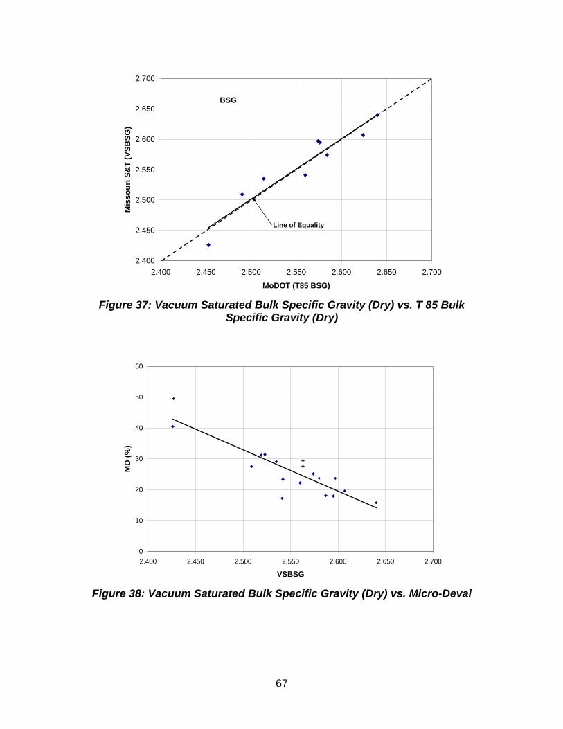
67

2.400

2.450

2.500

2.550

2.600

2.650

2.700

2.400 2.450 2.500 2.550 2.600 2.650 2.700

MoDOT (T85 BSG)

Mis

so

uri

S&

T (

VS

BS

G)

Line of Equality

BSG

Figure 37: Vacuum Saturated Bulk Specific Gravity (Dry) vs. T 85 Bulk

Specific Gravity (Dry)

0

10

20

30

40

50

60

2.400 2.450 2.500 2.550 2.600 2.650 2.700

VSBSG

MD

(%

)

Figure 38: Vacuum Saturated Bulk Specific Gravity (Dry) vs. Micro-Deval

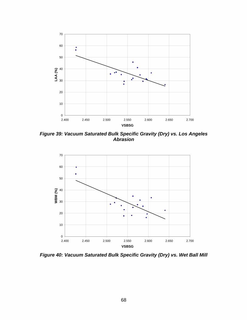
68

0

10

20

30

40

50

60

70

2.400 2.450 2.500 2.550 2.600 2.650 2.700

VSBSG

LA

A (

%)

Figure 39: Vacuum Saturated Bulk Specific Gravity (Dry) vs. Los Angeles

Abrasion

0

10

20

30

40

50

60

70

2.400 2.450 2.500 2.550 2.600 2.650 2.700

VSBSG

WB

M (

%)

Figure 40: Vacuum Saturated Bulk Specific Gravity (Dry) vs. Wet Ball Mill

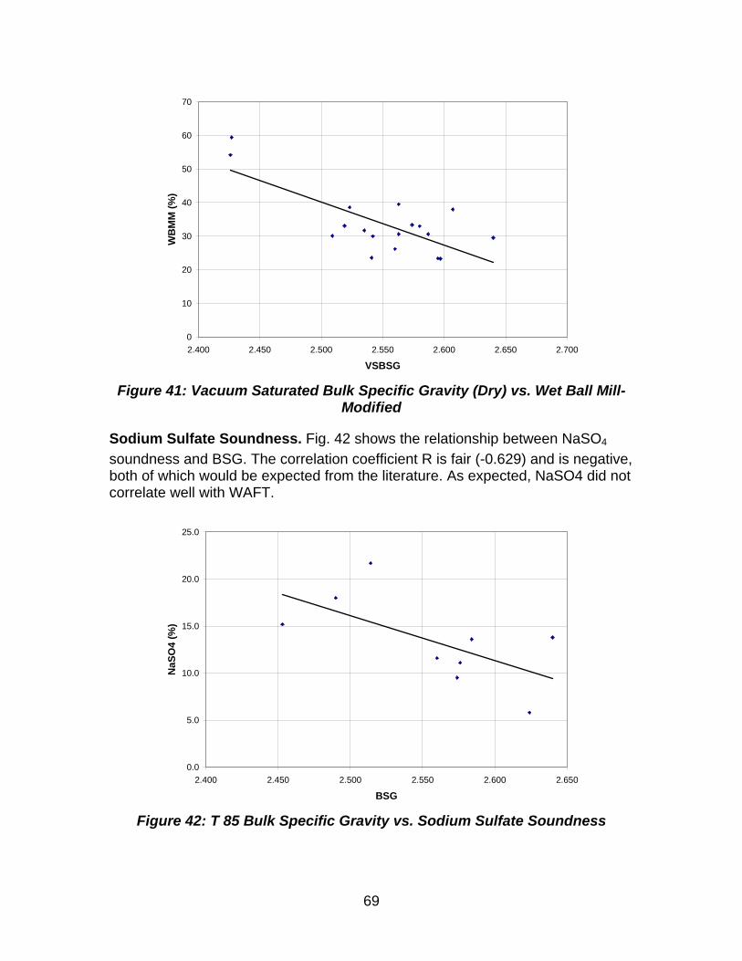
69

0

10

20

30

40

50

60

70

2.400 2.450 2.500 2.550 2.600 2.650 2.700

VSBSG

WB

MM

(%

)

Figure 41: Vacuum Saturated Bulk Specific Gravity (Dry) vs. Wet Ball Mill-

Modified

Sodium Sulfate Soundness. Fig. 42 shows the relationship between NaSO4

soundness and BSG. The correlation coefficient R is fair (-0.629) and is negative, both of which would be expected from the literature. As expected, NaSO4 did not correlate well with WAFT.

0.0

5.0

10.0

15.0

20.0

25.0

2.400 2.450 2.500 2.550 2.600 2.650

BSG

NaS

O4

(%)

Figure 42: T 85 Bulk Specific Gravity vs. Sodium Sulfate Soundness

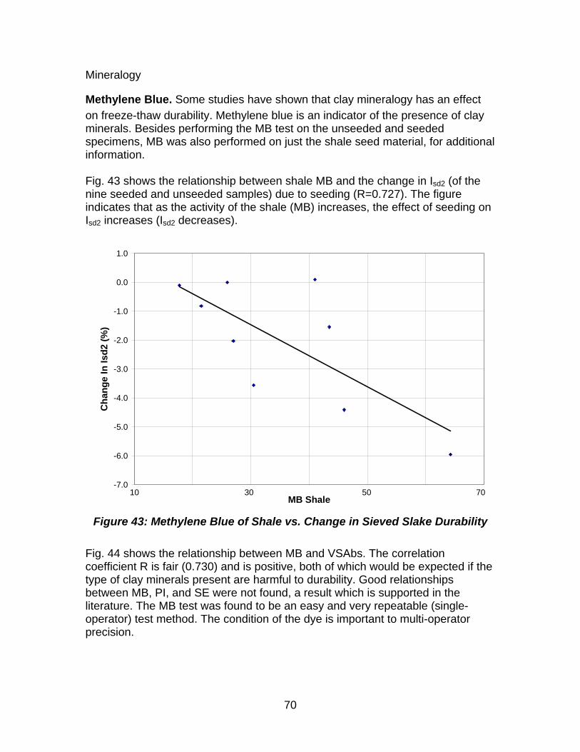
70

Mineralogy

Methylene Blue. Some studies have shown that clay mineralogy has an effect

on freeze-thaw durability. Methylene blue is an indicator of the presence of clay minerals. Besides performing the MB test on the unseeded and seeded specimens, MB was also performed on just the shale seed material, for additional information. Fig. 43 shows the relationship between shale MB and the change in Isd2 (of the nine seeded and unseeded samples) due to seeding (R=0.727). The figure indicates that as the activity of the shale (MB) increases, the effect of seeding on Isd2 increases (Isd2 decreases).

-7.0

-6.0

-5.0

-4.0

-3.0

-2.0

-1.0

0.0

1.0

MB Shale

Ch

ang

e I

n I

sd2

(%

)

10 30 50 70

Figure 43: Methylene Blue of Shale vs. Change in Sieved Slake Durability

Fig. 44 shows the relationship between MB and VSAbs. The correlation coefficient R is fair (0.730) and is positive, both of which would be expected if the type of clay minerals present are harmful to durability. Good relationships between MB, PI, and SE were not found, a result which is supported in the literature. The MB test was found to be an easy and very repeatable (single-operator) test method. The condition of the dye is important to multi-operator precision.

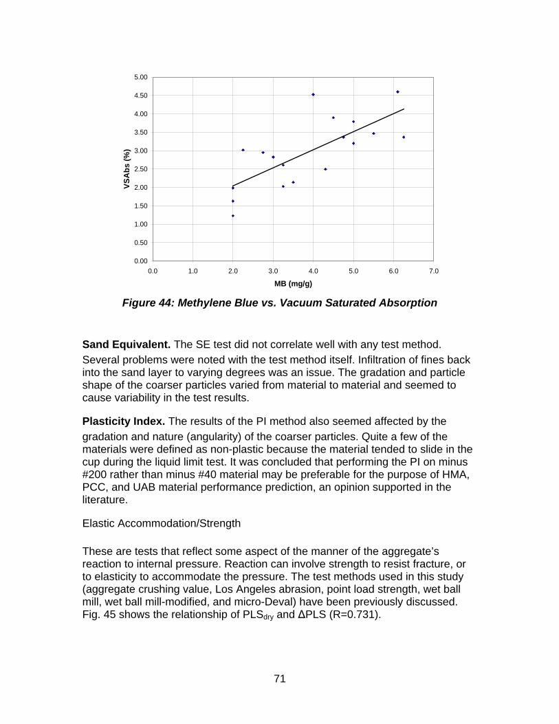
71

0.00

0.50

1.00

1.50

2.00

2.50

3.00

3.50

4.00

4.50

5.00

0.0 1.0 2.0 3.0 4.0 5.0 6.0 7.0

MB (mg/g)

VS

Ab

s (%

)

Figure 44: Methylene Blue vs. Vacuum Saturated Absorption

Sand Equivalent. The SE test did not correlate well with any test method.

Several problems were noted with the test method itself. Infiltration of fines back into the sand layer to varying degrees was an issue. The gradation and particle shape of the coarser particles varied from material to material and seemed to cause variability in the test results.

Plasticity Index. The results of the PI method also seemed affected by the

gradation and nature (angularity) of the coarser particles. Quite a few of the materials were defined as non-plastic because the material tended to slide in the cup during the liquid limit test. It was concluded that performing the PI on minus #200 rather than minus #40 material may be preferable for the purpose of HMA, PCC, and UAB material performance prediction, an opinion supported in the literature.

Elastic Accommodation/Strength

These are tests that reflect some aspect of the manner of the aggregate’s reaction to internal pressure. Reaction can involve strength to resist fracture, or to elasticity to accommodate the pressure. The test methods used in this study (aggregate crushing value, Los Angeles abrasion, point load strength, wet ball mill, wet ball mill-modified, and micro-Deval) have been previously discussed. Fig. 45 shows the relationship of PLSdry and ΔPLS (R=0.731).

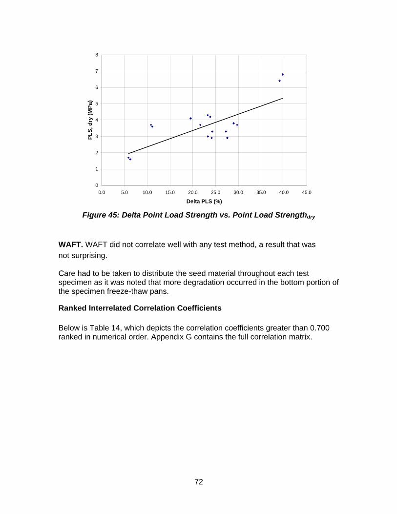
72

0

1

2

3

4

5

6

7

8

0.0 5.0 10.0 15.0 20.0 25.0 30.0 35.0 40.0 45.0

Delta PLS (%)

PL

S, d

ry (

MP

a)

Figure 45: Delta Point Load Strength vs. Point Load Strengthdry

WAFT. WAFT did not correlate well with any test method, a result that was

not surprising. Care had to be taken to distribute the seed material throughout each test specimen as it was noted that more degradation occurred in the bottom portion of the specimen freeze-thaw pans.

Ranked Interrelated Correlation Coefficients

Below is Table 14, which depicts the correlation coefficients greater than 0.700 ranked in numerical order. Appendix G contains the full correlation matrix.

73

Table 14: Interrelated Correlation Coefficients

Test Methods RWBM vs WBMM 0.990BSGod VS VSBSG 0.951LAA vs ACV 0.948WBM vs ACV 0.940LAA vs WBM 0.934PLSdry vs PLSwet 0.934LAA vs WBMM 0.931Abs vs VSAbs 0.926WBMM vs ACV 0.919MD vs LAA 0.892MD vs VSBSG -0.881MD vs WBM 0.873MD vs ACV 0.868MD vs WBMM 0.860MD vs BSGod -0.857BSGod vs Abs 0.848Abs vs VSBSG -0.816ACV vs PLSwet -0.807VSBSG vs VSAbs -0.800ACV vs PLSdry -0.791WBM vs PLSwet -0.768VSBSG vs LAA -0.764MD vs PLSwet -0.764VSBSG vs WBM -0.757WBMM vs VSBSG -0.737BSGod vs VSAbs -0.732DeltaPLS vs PLSdry 0.731MB vs VSAbs 0.730WBM vs PLSdry -0.728MBshale vs Isd2 -0.727WBMM vs PLSwet -0.710LAA vs PLSwet -0.710

Correlation with MoDOT Results

To see if Missouri S&T results lined up with historical test data from MoDOT, correlations were performed for tests that were common to both datasets. This involved LAA (R= 0.961), and to a limited extent, NaSO4 (0.599), and WAFT (0.039). Figs. 46 through 48 are shown below. In a comparison of vacuum saturated to T 85 types of test methods, BSG and Abs comparisons were discussed earlier and shown in Figs. 34 and 37. In general, considering that the MODOT and Missouri S&T tests were not performed on split samples, rather, the samples were taken months or even years apart, the test results seemed to correlate fairly well. Paired t-tests showed that, for each test method, there was no statistical difference between MoDOT’s and Missouri S&T’s results at the 0.05 α level. In regard to the NaSO4 results, there is one data point that appears to be

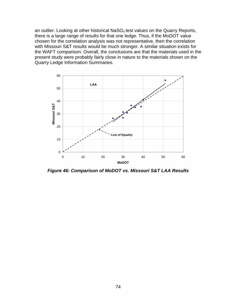
74

an outlier. Looking at other historical NaSO4 test values on the Quarry Reports, there is a large range of results for that one ledge. Thus, if the MoDOT value chosen for the correlation analysis was not representative, then the correlation with Missouri S&T results would be much stronger. A similar situation exists for the WAFT comparison. Overall, the conclusions are that the materials used in the present study were probably fairly close in nature to the materials shown on the Quarry Ledge Information Summaries.

0

10

20

30

40

50

60

0 10 20 30 40 50 60

MoDOT

Mis

sou

ri S

&T

Line of Equality

LAA

Figure 46: Comparison of MoDOT vs. Missouri S&T LAA Results

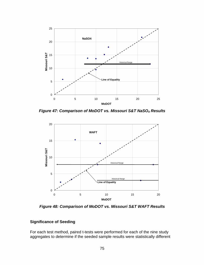
75

0

5

10

15

20

25

0 5 10 15 20 25

MoDOT

Mis

sou

ri S

&T

Line of Equality

NaSO4

Historical Range

Figure 47: Comparison of MoDOT vs. Missouri S&T NaSO4 Results

0

5

10

15

20

0 5 10 15 20

MoDOT

Mis

sou

ri S

&T

Line of Equality

WAFT

Historical Range

Historical Range

Figure 48: Comparison of MoDOT vs. Missouri S&T WAFT Results

Significance of Seeding For each test method, paired t-tests were performed for each of the nine study aggregates to determine if the seeded sample results were statistically different

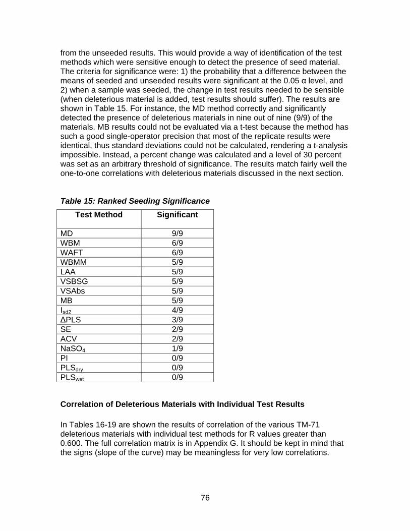
76

from the unseeded results. This would provide a way of identification of the test methods which were sensitive enough to detect the presence of seed material. The criteria for significance were: 1) the probability that a difference between the means of seeded and unseeded results were significant at the 0.05 α level, and 2) when a sample was seeded, the change in test results needed to be sensible (when deleterious material is added, test results should suffer). The results are shown in Table 15. For instance, the MD method correctly and significantly detected the presence of deleterious materials in nine out of nine (9/9) of the materials. MB results could not be evaluated via a t-test because the method has such a good single-operator precision that most of the replicate results were identical, thus standard deviations could not be calculated, rendering a t-analysis impossible. Instead, a percent change was calculated and a level of 30 percent was set as an arbitrary threshold of significance. The results match fairly well the one-to-one correlations with deleterious materials discussed in the next section. Table 15: Ranked Seeding Significance

Test Method Significant

MD 9/9 WBM 6/9 WAFT 6/9 WBMM 5/9 LAA 5/9 VSBSG 5/9 VSAbs 5/9 MB 5/9 Isd2 4/9 ΔPLS 3/9 SE 2/9 ACV 2/9 NaSO4 1/9 PI 0/9 PLSdry 0/9 PLSwet 0/9

Correlation of Deleterious Materials with Individual Test Results In Tables 16-19 are shown the results of correlation of the various TM-71 deleterious materials with individual test methods for R values greater than 0.600. The full correlation matrix is in Appendix G. It should be kept in mind that the signs (slope of the curve) may be meaningless for very low correlations.

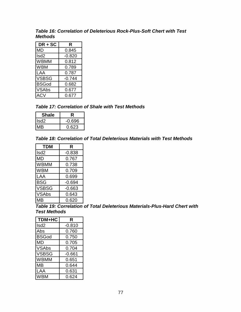
77

Table 16: Correlation of Deleterious Rock-Plus-Soft Chert with Test Methods

DR + SC RMD 0.845Isd2 -0.820WBMM 0.812WBM 0.789LAA 0.787VSBSG -0.744BSGod 0.682VSAbs 0.677ACV

0.677

Table 17: Correlation of Shale with Test Methods

Shale RIsd2 -0.696MB 0.623 Table 18: Correlation of Total Deleterious Materials with Test Methods

TDM RIsd2 -0.838MD 0.767WBMM 0.738WBM 0.709LAA 0.699BSG -0.694VSBSG -0.663VSAbs 0.643MB 0.620 Table 19: Correlation of Total Deleterious Materials-Plus-Hard Chert with Test Methods

TDM+HC RIsd2 -0.810Abs 0.760BSGod 0.750MD 0.705VSAbs 0.704VSBSG -0.661WBMM 0.651MB 0.644LAA 0.631WBM 0.624

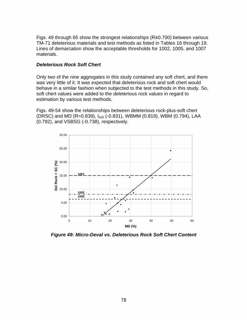
78

Figs. 49 through 65 show the strongest relationships (R≥0.700) between various TM-71 deleterious materials and test methods as listed in Tables 16 through 19. Lines of demarcation show the acceptable thresholds for 1002, 1005, and 1007 materials.

Deleterious Rock Soft Chert

Only two of the nine aggregates in this study contained any soft chert, and there was very little of it. It was expected that deleterious rock and soft chert would behave in a similar fashion when subjected to the test methods in this study. So, soft chert values were added to the deleterious rock values in regard to estimation by various test methods. Figs. 49-54 show the relationships between deleterious rock-plus-soft chert (DRSC) and MD (R=0.839), Isd2 (-0.831), WBMM (0.819), WBM (0.794), LAA (0.792), and VSBSG (-0.738), respectively.

0.00

5.00

10.00

15.00

20.00

25.00

30.00

0 10 20 30 40 50 60

MD (%)

Del

Ro

ck +

SC

(%

)

10051002

1007

Figure 49: Micro-Deval vs. Deleterious Rock Soft Chert Content

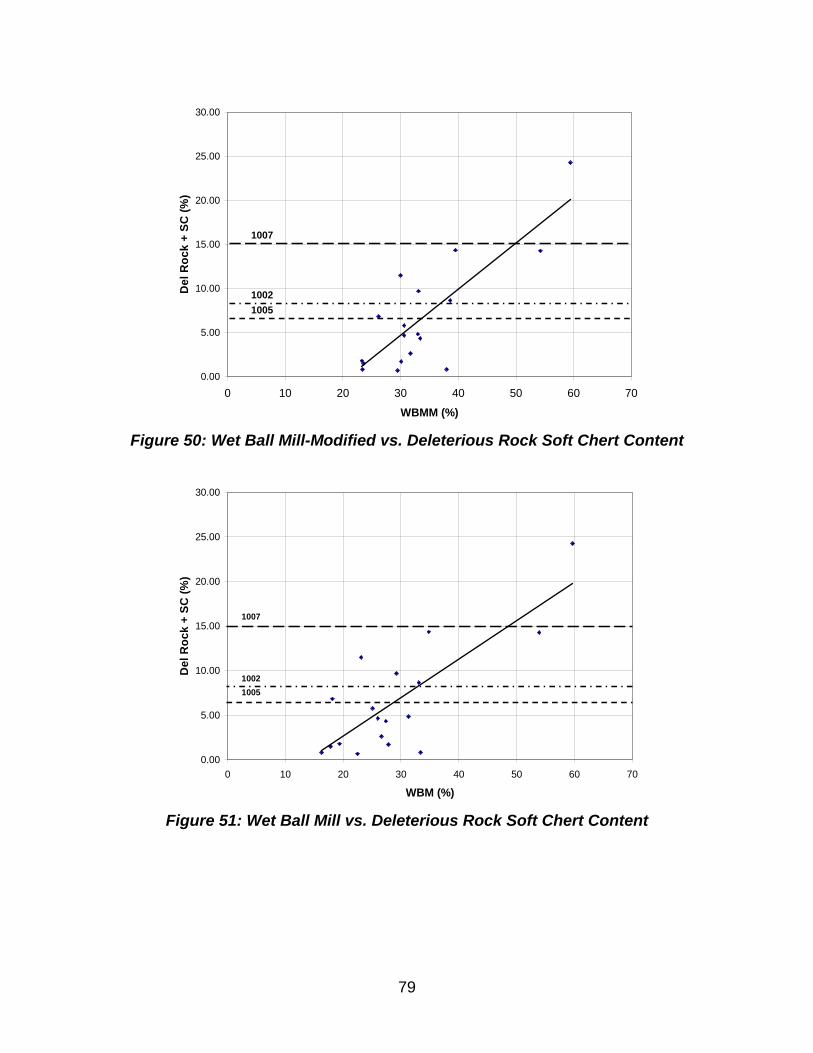
79

0.00

5.00

10.00

15.00

20.00

25.00

30.00

0 10 20 30 40 50 60 70

WBMM (%)

Del

Ro

ck +

SC

(%

)

1005

1002

1007

Figure 50: Wet Ball Mill-Modified vs. Deleterious Rock Soft Chert Content

0.00

5.00

10.00

15.00

20.00

25.00

30.00

0 10 20 30 40 50 60 70

WBM (%)

Del

Ro

ck +

SC

(%

)

1005

1002

1007

Figure 51: Wet Ball Mill vs. Deleterious Rock Soft Chert Content

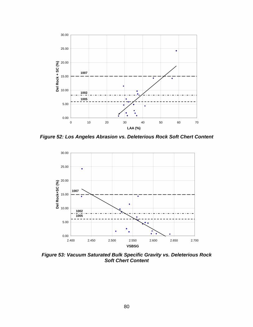
80

0.00

5.00

10.00

15.00

20.00

25.00

30.00

0 10 20 30 40 50 60 70

LAA (%)

Del

Ro

ck +

SC

(%

)

1005

1002

1007

Figure 52: Los Angeles Abrasion vs. Deleterious Rock Soft Chert Content

0.00

5.00

10.00

15.00

20.00

25.00

30.00

2.400 2.450 2.500 2.550 2.600 2.650 2.700

VSBSG

Del

Ro

ck+

SC

(%

)

1005

1002

1007

Figure 53: Vacuum Saturated Bulk Specific Gravity vs. Deleterious Rock

Soft Chert Content

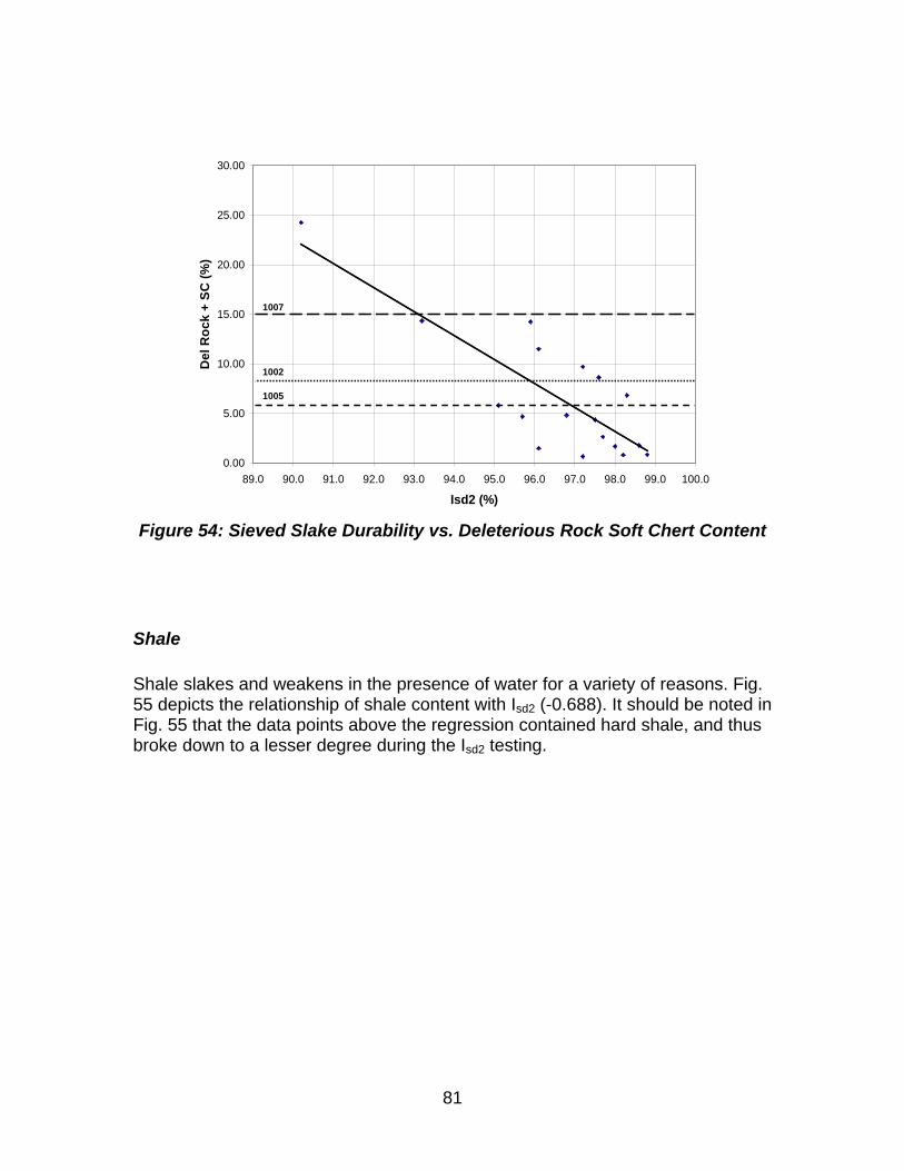
81

0.00

5.00

10.00

15.00

20.00

25.00

30.00

89.0 90.0 91.0 92.0 93.0 94.0 95.0 96.0 97.0 98.0 99.0 100.0

Isd2 (%)

Del

Ro

ck +

SC

(%

)

1007

1002

1005

Figure 54: Sieved Slake Durability vs. Deleterious Rock Soft Chert Content

Shale Shale slakes and weakens in the presence of water for a variety of reasons. Fig. 55 depicts the relationship of shale content with Isd2 (-0.688). It should be noted in Fig. 55 that the data points above the regression contained hard shale, and thus broke down to a lesser degree during the Isd2 testing.

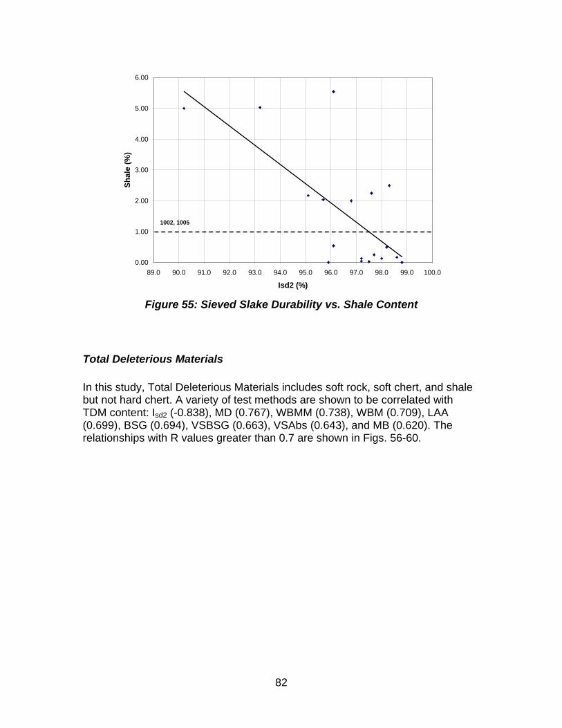
82

0.00

1.00

2.00

3.00

4.00

5.00

6.00

89.0 90.0 91.0 92.0 93.0 94.0 95.0 96.0 97.0 98.0 99.0 100.0

Isd2 (%)

Sh

ale

(%

)

1002, 1005

Figure 55: Sieved Slake Durability vs. Shale Content

Total Deleterious Materials

In this study, Total Deleterious Materials includes soft rock, soft chert, and shale but not hard chert. A variety of test methods are shown to be correlated with TDM content: Isd2 (-0.838), MD (0.767), WBMM (0.738), WBM (0.709), LAA (0.699), BSG (0.694), VSBSG (0.663), VSAbs (0.643), and MB (0.620). The relationships with R values greater than 0.7 are shown in Figs. 56-60.

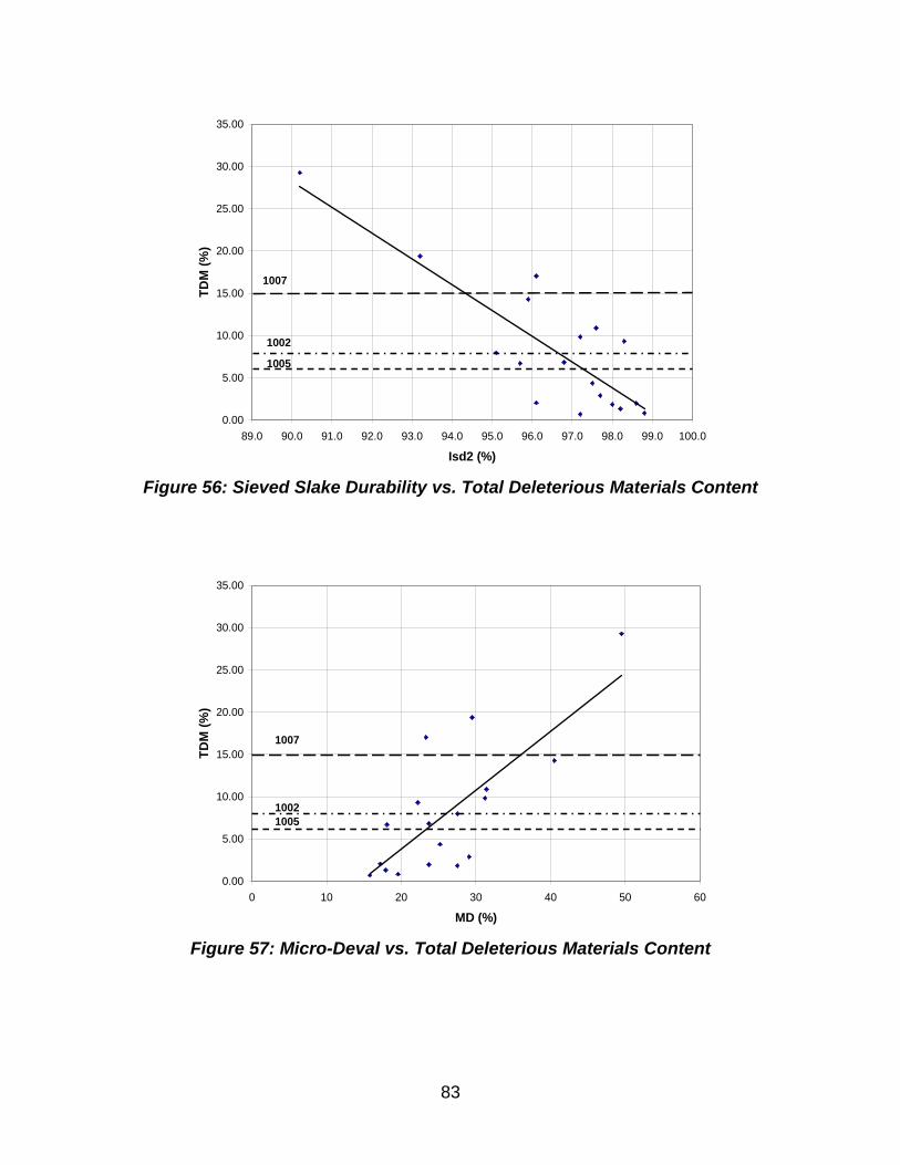
83

0.00

5.00

10.00

15.00

20.00

25.00

30.00

35.00

89.0 90.0 91.0 92.0 93.0 94.0 95.0 96.0 97.0 98.0 99.0 100.0

Isd2 (%)

TD

M (

%)

1005

1002

1007

Figure 56: Sieved Slake Durability vs. Total Deleterious Materials Content

0.00

5.00

10.00

15.00

20.00

25.00

30.00

35.00

0 10 20 30 40 50 60

MD (%)

TD

M (

%)

10051002

1007

Figure 57: Micro-Deval vs. Total Deleterious Materials Content

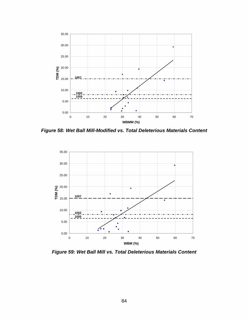
84

0.00

5.00

10.00

15.00

20.00

25.00

30.00

35.00

0 10 20 30 40 50 60 70

WBMM (%)

TD

M (

%)

10051002

1007

Figure 58: Wet Ball Mill-Modified vs. Total Deleterious Materials Content

0.00

5.00

10.00

15.00

20.00

25.00

30.00

35.00

0 10 20 30 40 50 60 70

WBM (%)

TD

M (

%)

10051002

1007

Figure 59: Wet Ball Mill vs. Total Deleterious Materials Content

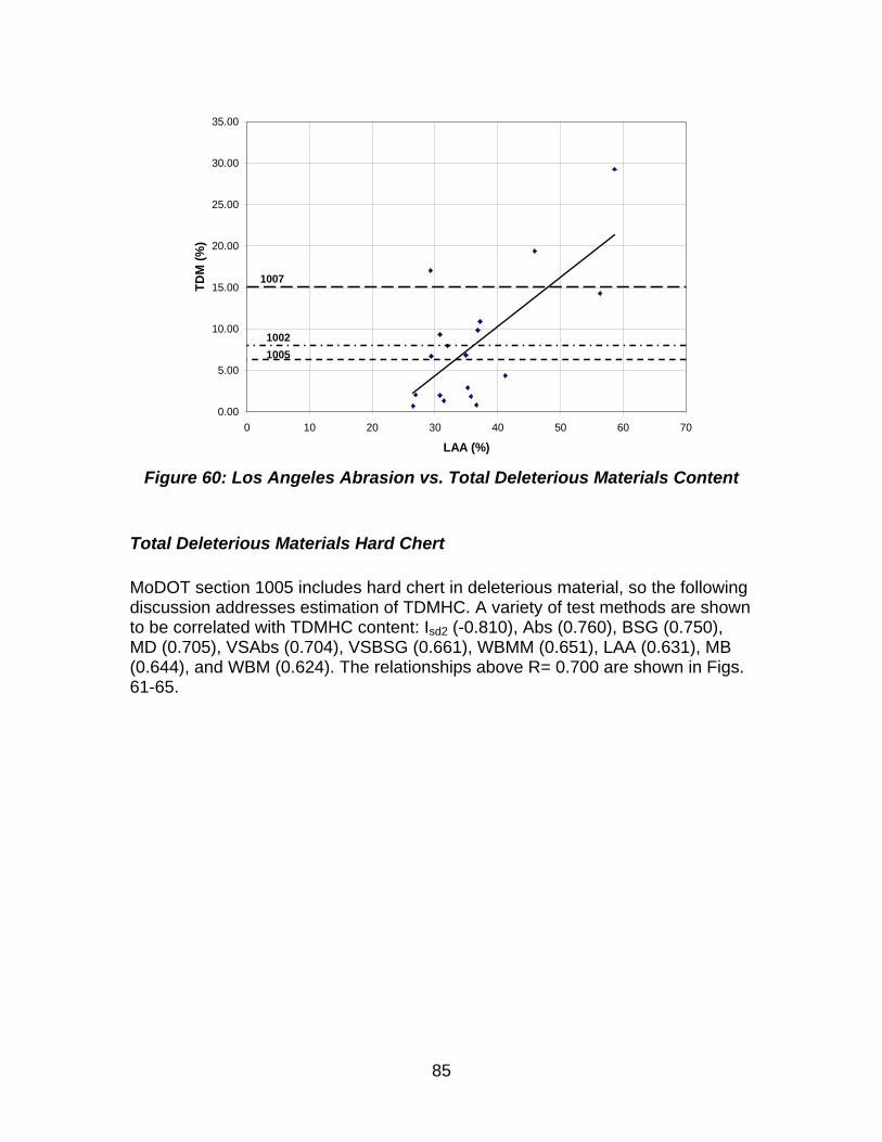
85

0.00

5.00

10.00

15.00

20.00

25.00

30.00

35.00

0 10 20 30 40 50 60 70

LAA (%)

TD

M (

%)

1005

1002

1007

Figure 60: Los Angeles Abrasion vs. Total Deleterious Materials Content

Total Deleterious Materials Hard Chert MoDOT section 1005 includes hard chert in deleterious material, so the following discussion addresses estimation of TDMHC. A variety of test methods are shown to be correlated with TDMHC content: Isd2 (-0.810), Abs (0.760), BSG (0.750), MD (0.705), VSAbs (0.704), VSBSG (0.661), WBMM (0.651), LAA (0.631), MB (0.644), and WBM (0.624). The relationships above R= 0.700 are shown in Figs. 61-65.

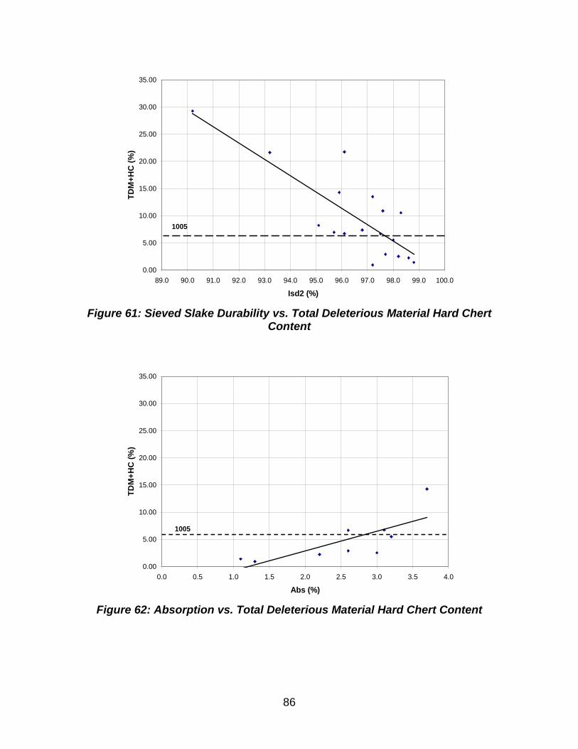
86

0.00

5.00

10.00

15.00

20.00

25.00

30.00

35.00

89.0 90.0 91.0 92.0 93.0 94.0 95.0 96.0 97.0 98.0 99.0 100.0

Isd2 (%)

TD

M+

HC

(%

)

1005

Figure 61: Sieved Slake Durability vs. Total Deleterious Material Hard Chert

Content

0.00

5.00

10.00

15.00

20.00

25.00

30.00

35.00

0.0 0.5 1.0 1.5 2.0 2.5 3.0 3.5 4.0

Abs (%)

TD

M+

HC

(%

)

1005

Figure 62: Absorption vs. Total Deleterious Material Hard Chert Content

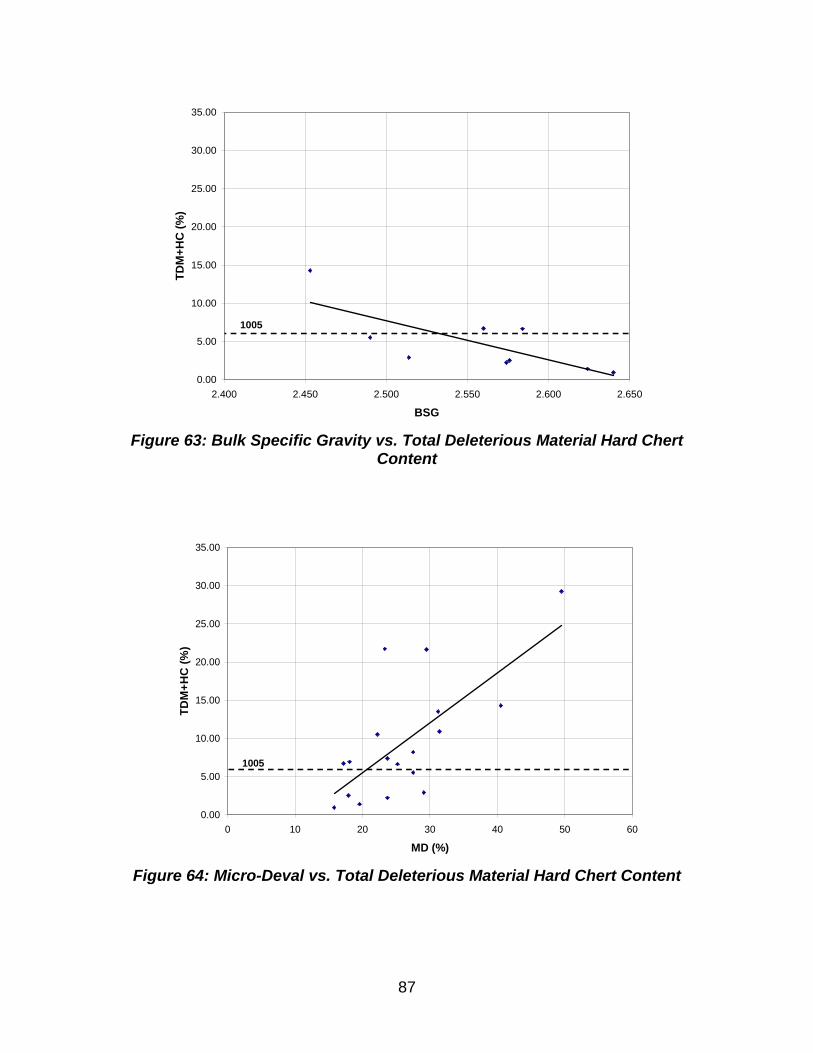
87

0.00

5.00

10.00

15.00

20.00

25.00

30.00

35.00

2.400 2.450 2.500 2.550 2.600 2.650

BSG

TD

M+

HC

(%

)

1005

Figure 63: Bulk Specific Gravity vs. Total Deleterious Material Hard Chert

Content

0.00

5.00

10.00

15.00

20.00

25.00

30.00

35.00

0 10 20 30 40 50 60

MD (%)

TD

M+

HC

(%

)

1005

Figure 64: Micro-Deval vs. Total Deleterious Material Hard Chert Content

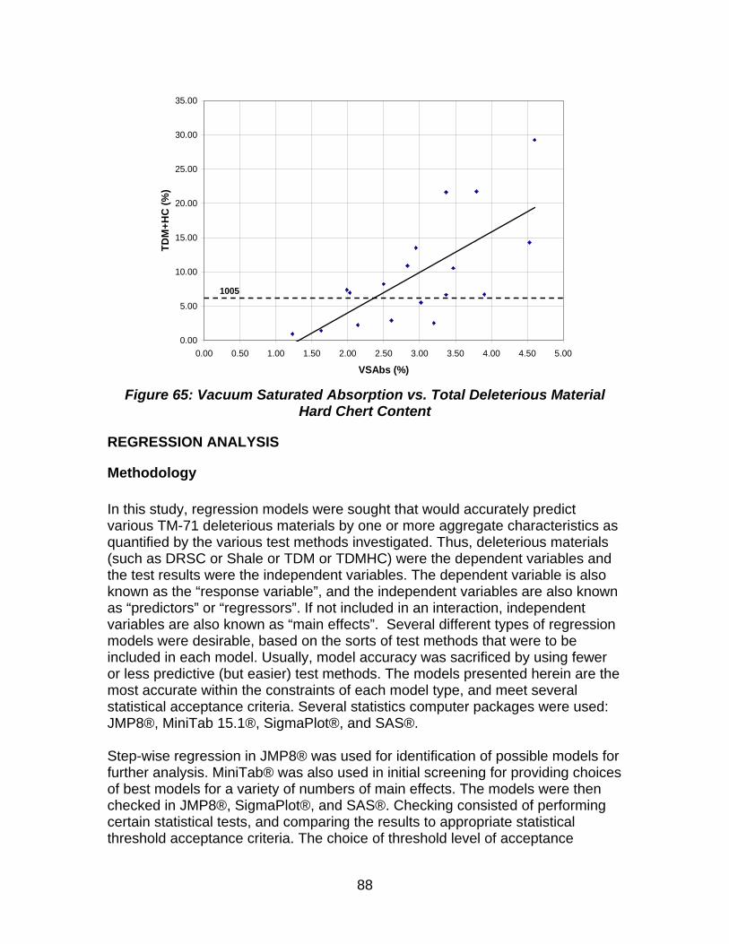
88

0.00

5.00

10.00

15.00

20.00

25.00

30.00

35.00

0.00 0.50 1.00 1.50 2.00 2.50 3.00 3.50 4.00 4.50 5.00

VSAbs (%)

TD

M+

HC

(%

)

1005

Figure 65: Vacuum Saturated Absorption vs. Total Deleterious Material

Hard Chert Content

REGRESSION ANALYSIS

Methodology

In this study, regression models were sought that would accurately predict various TM-71 deleterious materials by one or more aggregate characteristics as quantified by the various test methods investigated. Thus, deleterious materials (such as DRSC or Shale or TDM or TDMHC) were the dependent variables and the test results were the independent variables. The dependent variable is also known as the “response variable”, and the independent variables are also known as “predictors” or “regressors”. If not included in an interaction, independent variables are also known as “main effects”. Several different types of regression models were desirable, based on the sorts of test methods that were to be included in each model. Usually, model accuracy was sacrificed by using fewer or less predictive (but easier) test methods. The models presented herein are the most accurate within the constraints of each model type, and meet several statistical acceptance criteria. Several statistics computer packages were used: JMP8®, MiniTab 15.1®, SigmaPlot®, and SAS®. Step-wise regression in JMP8® was used for identification of possible models for further analysis. MiniTab® was also used in initial screening for providing choices of best models for a variety of numbers of main effects. The models were then checked in JMP8®, SigmaPlot®, and SAS®. Checking consisted of performing certain statistical tests, and comparing the results to appropriate statistical threshold acceptance criteria. The choice of threshold level of acceptance

89

conformed to typical practice. Generally, the most accurate model that passed all the tests was the model of choice for a given type of deleterious material.

Model Acceptance Criteria

Seven statistical criteria were used for model acceptance: one criterion for ranking models and the other six for checking for possible problems.

R2 The “R2 “(coefficient of determination) of a regression model is a measure of the fit with the sample data. It is the proportion of Y variability that can be predicted from X in the sample (Schulman, 1992). As the R2 increases, the fit of the model improves.

Adjusted R2

The “adjusted R2 “of a regression model is a measure of the fit with the population data. Adjusted R2 is a superior statistic to R2 during model selection because it takes into account the varying numbers of independent variables so as to not falsely inflate R2. For each type of model, the one ultimately chosen in this study was the one with the highest adjusted R2 that met all the criteria listed below. Reviewers who are more familiar with working with R2 should note that adjusted R2 values are always lower than R2 values (predictions in the population are always worse than in the sample), so one must adjust one’s frame of reference.

Significance of Model

Each model must show that it fits the data, and thus is significant, at the 0.01 α level. The analysis of variance F-statistic will indicate this condition.

Term Significance

Each term in a regression equation must be significant at an α= 0.05 level.

Multi-Collinearity

Multi-collinearity must be minimized in order to increase stability of the equation. For example, if two or more main effects are highly collinear, then unstable predictions may be made by the equation. Thus, only one of the collinear predictor variables should be allowed to remain in the equation. Multi-collinearity was assessed by two test statistics: Variance Inflation Factor (VIF) and Condition Number (CN). VIFs are measured for each variable in the equation. A threshold level generally preferred is 4 or less, with 5 being an upper limit. CNs are global; one CN is assigned to the entire equation. A desirable CN is 30 or less.

90

Undue Influence of Single Data Points

Single observations should not be allowed to influence the regression unduly. An observation in regression analysis is defined as all the data that predicts a single response value. In other words, an observation would be a row of data points (i.e. test results) in Tables 10-13 that is associated with the single deleterious material parameter, e.g. DRSC. Thus, there were 18 observations in this study. Any data point within a given observation could cause the excessive influence. Influence is measured by DFFITS (Difference in Fits), which is the change in a given predicted value when the observation being tested is removed from the data set and the model is re-fit to the remaining data. A desirable value of DFFITS used in this study was 2.0 standard deviations or less. High DFFITS values should be explored to determine if any action is deemed necessary in regard to rejecting an observation. Usually, a conservative approach is to retain the observation unless there is a compelling reason to reject an outlier.

Normality of Test Residuals A residual is the error (difference) between an actual (observed or measured) single response variable value (e.g. TDM) and the associated predicted value for a given regression model. The residuals should be normally distributed. Meeting normality criteria checks the assumption of regression modeling that residuals are indeed normal. Normality was checked with the Kolmogorov-Smirnov test at a significance level of 95%.

Constant Variance of Residuals Residuals should also be checked to make sure that the magnitudes of the residuals are relatively uniform throughout the entire range of data. Again, this is just a check of another assumption that is part of regression analysis. Constant variance was checked with the Spearman rank correlation test at a significance level of 95%.

Regression Models The following are the regression models that were considered to have the most application for MoDOT’s use. MoDOT can choose the model(s) that will work best under various conditions. Options that are presented involve choosing test methods based on familiarity, willingness to start something new, equipment cost, sensitivity to test duration, the level of accuracy that is considered acceptable, plus the overall predictive system ease of use. A common set of test types usually surfaced as the best predictors for each category of model.

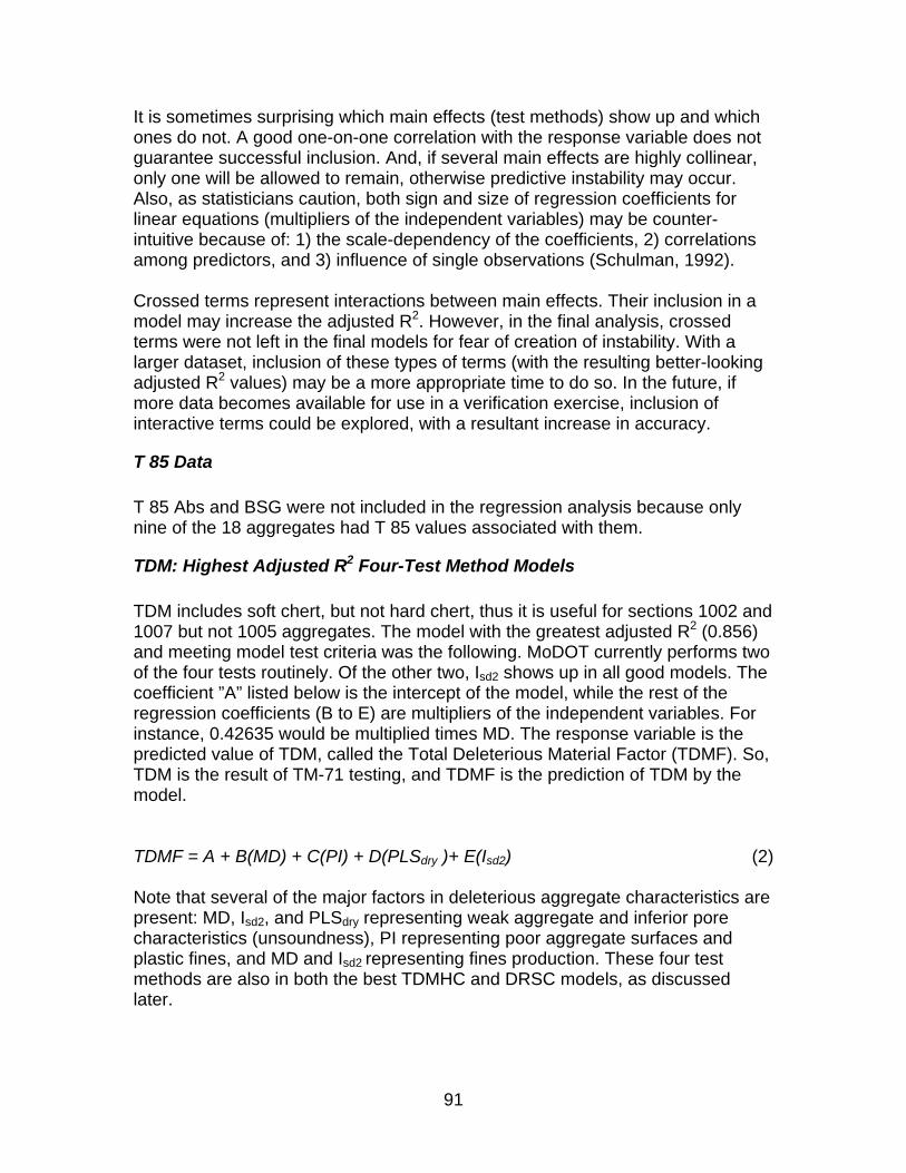
91

It is sometimes surprising which main effects (test methods) show up and which ones do not. A good one-on-one correlation with the response variable does not guarantee successful inclusion. And, if several main effects are highly collinear, only one will be allowed to remain, otherwise predictive instability may occur. Also, as statisticians caution, both sign and size of regression coefficients for linear equations (multipliers of the independent variables) may be counter-intuitive because of: 1) the scale-dependency of the coefficients, 2) correlations among predictors, and 3) influence of single observations (Schulman, 1992). Crossed terms represent interactions between main effects. Their inclusion in a model may increase the adjusted R2. However, in the final analysis, crossed terms were not left in the final models for fear of creation of instability. With a larger dataset, inclusion of these types of terms (with the resulting better-looking adjusted R2 values) may be a more appropriate time to do so. In the future, if more data becomes available for use in a verification exercise, inclusion of interactive terms could be explored, with a resultant increase in accuracy.

T 85 Data

T 85 Abs and BSG were not included in the regression analysis because only nine of the 18 aggregates had T 85 values associated with them.

TDM: Highest Adjusted R2 Four-Test Method Models

TDM includes soft chert, but not hard chert, thus it is useful for sections 1002 and 1007 but not 1005 aggregates. The model with the greatest adjusted R2 (0.856) and meeting model test criteria was the following. MoDOT currently performs two of the four tests routinely. Of the other two, Isd2 shows up in all good models. The coefficient ”A” listed below is the intercept of the model, while the rest of the regression coefficients (B to E) are multipliers of the independent variables. For instance, 0.42635 would be multiplied times MD. The response variable is the predicted value of TDM, called the Total Deleterious Material Factor (TDMF). So, TDM is the result of TM-71 testing, and TDMF is the prediction of TDM by the model. TDMF = A + B(MD) + C(PI) + D(PLSdry )+ E(Isd2) (2) Note that several of the major factors in deleterious aggregate characteristics are present: MD, Isd2, and PLSdry representing weak aggregate and inferior pore characteristics (unsoundness), PI representing poor aggregate surfaces and plastic fines, and MD and Isd2 representing fines production. These four test methods are also in both the best TDMHC and DRSC models, as discussed later.

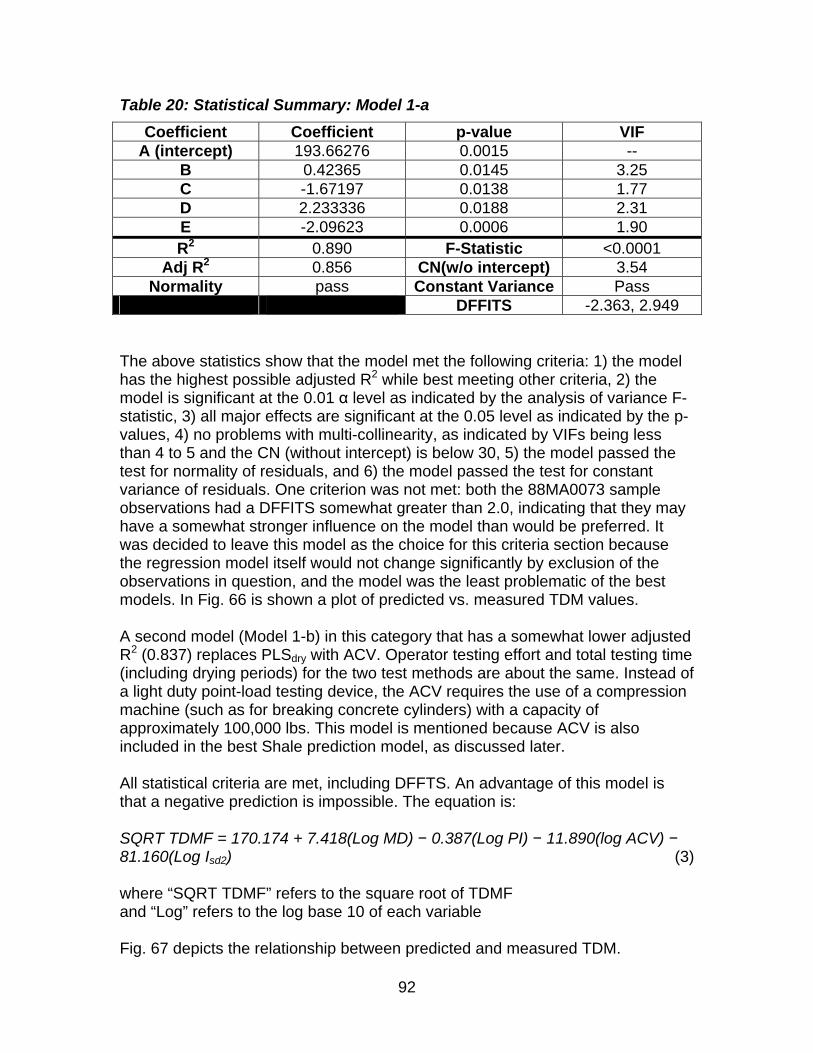
92

Table 20: Statistical Summary: Model 1-a

Coefficient Coefficient p-value VIF A (intercept) 193.66276 0.0015 --

B 0.42365 0.0145 3.25 C -1.67197 0.0138 1.77 D 2.233336 0.0188 2.31 E -2.09623 0.0006 1.90 R2 0.890 F-Statistic <0.0001

Adj R2 0.856 CN(w/o intercept) 3.54 Normality pass Constant Variance Pass

DFFITS -2.363, 2.949 The above statistics show that the model met the following criteria: 1) the model has the highest possible adjusted R2 while best meeting other criteria, 2) the model is significant at the 0.01 α level as indicated by the analysis of variance F-statistic, 3) all major effects are significant at the 0.05 level as indicated by the p-values, 4) no problems with multi-collinearity, as indicated by VIFs being less than 4 to 5 and the CN (without intercept) is below 30, 5) the model passed the test for normality of residuals, and 6) the model passed the test for constant variance of residuals. One criterion was not met: both the 88MA0073 sample observations had a DFFITS somewhat greater than 2.0, indicating that they may have a somewhat stronger influence on the model than would be preferred. It was decided to leave this model as the choice for this criteria section because the regression model itself would not change significantly by exclusion of the observations in question, and the model was the least problematic of the best models. In Fig. 66 is shown a plot of predicted vs. measured TDM values. A second model (Model 1-b) in this category that has a somewhat lower adjusted R2 (0.837) replaces PLSdry with ACV. Operator testing effort and total testing time (including drying periods) for the two test methods are about the same. Instead of a light duty point-load testing device, the ACV requires the use of a compression machine (such as for breaking concrete cylinders) with a capacity of approximately 100,000 lbs. This model is mentioned because ACV is also included in the best Shale prediction model, as discussed later. All statistical criteria are met, including DFFTS. An advantage of this model is that a negative prediction is impossible. The equation is: SQRT TDMF = 170.174 + 7.418(Log MD) − 0.387(Log PI) − 11.890(log ACV) − 81.160(Log Isd2) (3) where “SQRT TDMF” refers to the square root of TDMF and “Log” refers to the log base 10 of each variable Fig. 67 depicts the relationship between predicted and measured TDM.

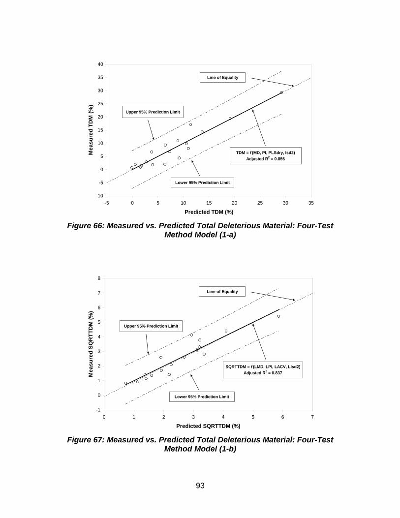
93

-10

-5

0

5

10

15

20

25

30

35

40

-5 0 5 10 15 20 25 30 35

Predicted TDM (%)

Mea

sure

d T

DM

(%

)

TDM = f (MD, PI, PLSdry, Isd2)

Adjusted R2 = 0.856

Upper 95% Prediction Limit

Lower 95% Prediction Limit

Line of Equality

Figure 66: Measured vs. Predicted Total Deleterious Material: Four-Test

Method Model (1-a)

-1

0

1

2

3

4

5

6

7

8

0 1 2 3 4 5 6 7

Predicted SQRTTDM (%)

Mea

sure

d S

QR

TT

DM

(%

)

SQRTTDM = f (LMD, LPI, LACV, LIsd2)

Adjusted R2 = 0.837



Line of Equality

Figure 67: Measured vs. Predicted Total Deleterious Material: Four-Test

Method Model (1-b)

94

TDM: Highest Adjusted R2 Three-Test Method Model

The best three-test method model (Model 1-c), with an adjusted R2 = 0.822, is the following. All criteria were met. This model introduces VSAbs. This method is the same as the T 85 method, but with an introductory vacuum saturation step. Some deleterious aggregate characteristics appear to not be as well-represented as in the four-test method models. TDMF = 238.52245 – 1.42354(PI) – 2.42891(Isd2) + 2.12781(VSAbs) (4) In Fig. 68 is shown a plot of predicted vs. measured TDM values.

-10

-5

0

5

10

15

20

25

30

35

40

-5 0 5 10 15 20 25 30 35

Predicted TDM (%)

Mea

sure

d T

DM

(%

)

TDM = f (PI, Isd2, VSAbs)

Adjusted R2 = 0.822



Line of Equality

Figure 68: Measured vs. Predicted Total Deleterious Material: Three-Test

Method Model (1-c)

TDM: Two-Test Method Model

Although not the best two-test model, one that offers some different kinds of test methods is Model 1-d, which features WBM and MB (adjusted R2 = 0.741). All criteria were met. Some deleterious aggregate characteristics appear to not be as well-represented as in the four-test method models. TDMF = −15.373 + 0.424(WBM) + 2.905(MB) (5)

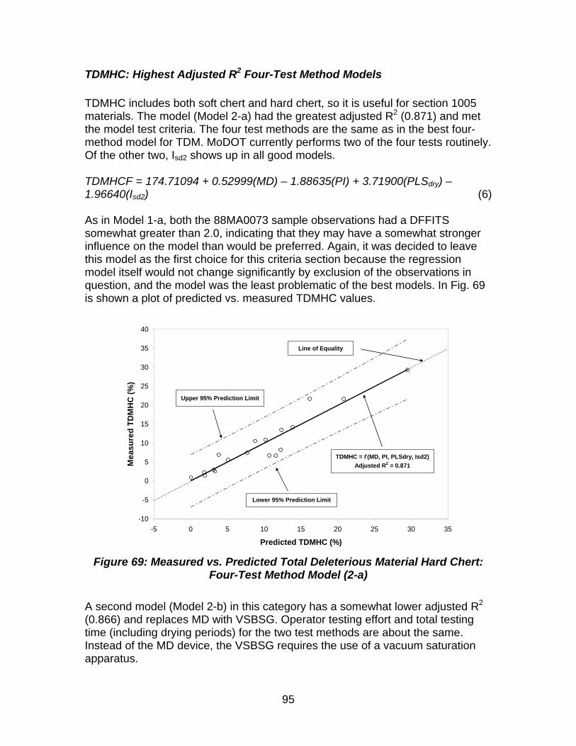
95

TDMHC: Highest Adjusted R2 Four-Test Method Models

TDMHC includes both soft chert and hard chert, so it is useful for section 1005 materials. The model (Model 2-a) had the greatest adjusted R2 (0.871) and met the model test criteria. The four test methods are the same as in the best four-method model for TDM. MoDOT currently performs two of the four tests routinely. Of the other two, Isd2 shows up in all good models. TDMHCF = 174.71094 + 0.52999(MD) – 1.88635(PI) + 3.71900(PLSdry) – 1.96640(Isd2) (6) As in Model 1-a, both the 88MA0073 sample observations had a DFFITS somewhat greater than 2.0, indicating that they may have a somewhat stronger influence on the model than would be preferred. Again, it was decided to leave this model as the first choice for this criteria section because the regression model itself would not change significantly by exclusion of the observations in question, and the model was the least problematic of the best models. In Fig. 69 is shown a plot of predicted vs. measured TDMHC values.

-10

-5

0

5

10

15

20

25

30

35

40

-5 0 5 10 15 20 25 30 35

Predicted TDMHC (%)

Mea

sure

d T

DM

HC

(%

)

TDMHC = f (MD, PI, PLSdry, Isd2)

Adjusted R2 = 0.871



Line of Equality

Figure 69: Measured vs. Predicted Total Deleterious Material Hard Chert:

Four-Test Method Model (2-a)

A second model (Model 2-b) in this category has a somewhat lower adjusted R2 (0.866) and replaces MD with VSBSG. Operator testing effort and total testing time (including drying periods) for the two test methods are about the same. Instead of the MD device, the VSBSG requires the use of a vacuum saturation apparatus.

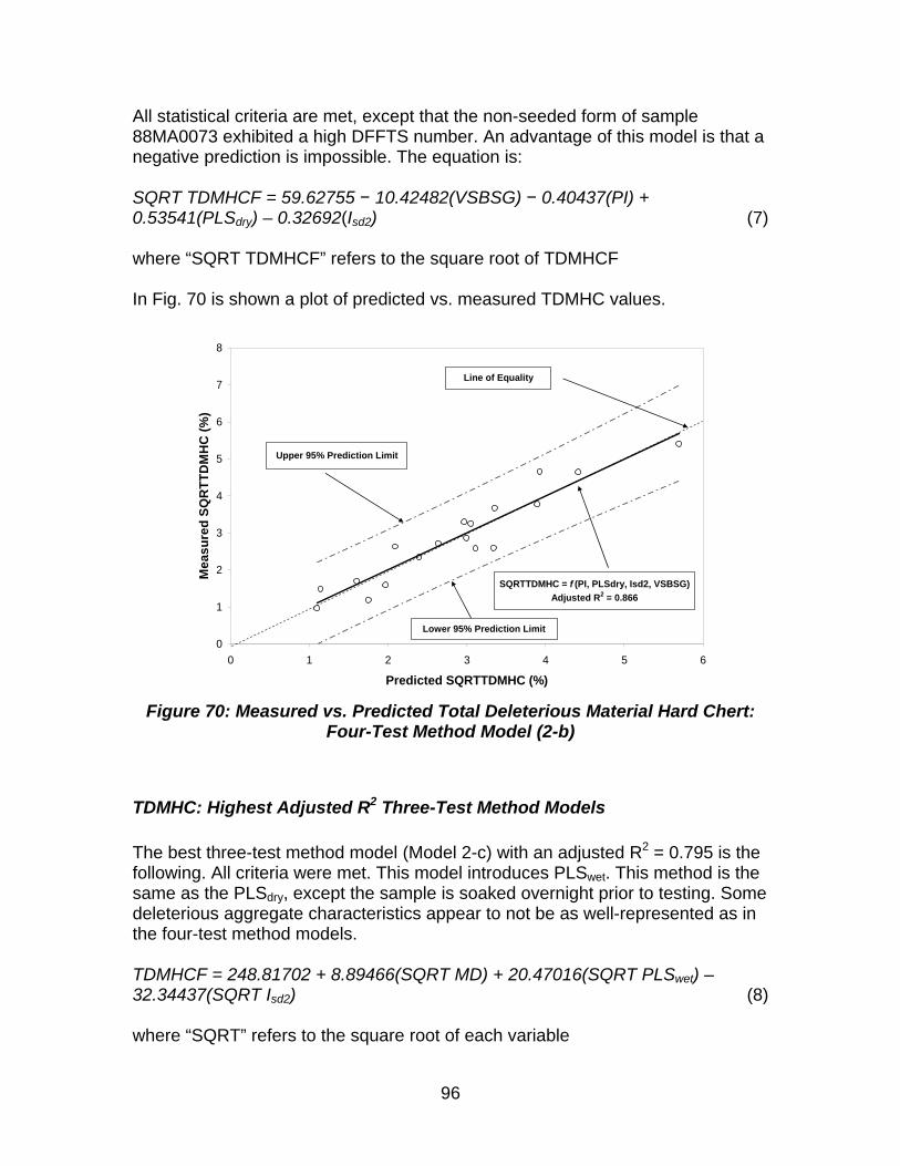
96

All statistical criteria are met, except that the non-seeded form of sample 88MA0073 exhibited a high DFFTS number. An advantage of this model is that a negative prediction is impossible. The equation is: SQRT TDMHCF = 59.62755 − 10.42482(VSBSG) − 0.40437(PI) + 0.53541(PLSdry) – 0.32692(Isd2) (7) where “SQRT TDMHCF” refers to the square root of TDMHCF In Fig. 70 is shown a plot of predicted vs. measured TDMHC values.

0

1

2

3

4

5

6

7

8

0 1 2 3 4 5 6

Predicted SQRTTDMHC (%)

Mea

sure

d S

QR

TT

DM

HC

(%

)

SQRTTDMHC = f (PI, PLSdry, Isd2, VSBSG)

Adjusted R2 = 0.866



Line of Equality


Four-Test Method Model (2-b)

TDMHC: Highest Adjusted R2 Three-Test Method Models

The best three-test method model (Model 2-c) with an adjusted R2 = 0.795 is the following. All criteria were met. This model introduces PLSwet. This method is the same as the PLSdry, except the sample is soaked overnight prior to testing. Some deleterious aggregate characteristics appear to not be as well-represented as in the four-test method models. TDMHCF = 248.81702 + 8.89466(SQRT MD) + 20.47016(SQRT PLSwet) – 32.34437(SQRT Isd2) (8) where “SQRT” refers to the square root of each variable

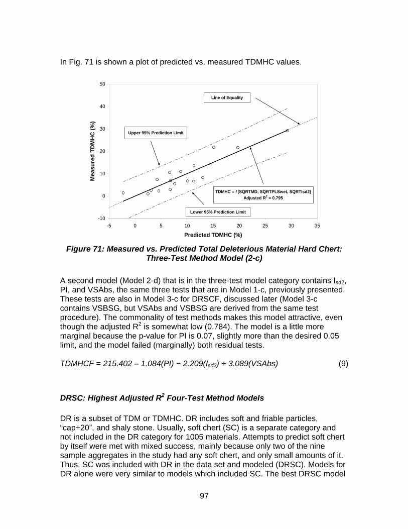
97

In Fig. 71 is shown a plot of predicted vs. measured TDMHC values.

-10

0

10

20

30

40

50

-5 0 5 10 15 20 25 30 35

Predicted TDMHC (%)

Mea

sure

d T

DM

HC

(%

)

TDMHC = f (SQRTMD, SQRTPLSwet, SQRTIsd2)

Adjusted R2 = 0.795



Line of Equality


Three-Test Method Model (2-c)

A second model (Model 2-d) that is in the three-test model category contains Isd2, PI, and VSAbs, the same three tests that are in Model 1-c, previously presented. These tests are also in Model 3-c for DRSCF, discussed later (Model 3-c contains VSBSG, but VSAbs and VSBSG are derived from the same test procedure). The commonality of test methods makes this model attractive, even though the adjusted R2 is somewhat low (0.784). The model is a little more marginal because the p-value for PI is 0.07, slightly more than the desired 0.05 limit, and the model failed (marginally) both residual tests. TDMHCF = 215.402 – 1.084(PI) − 2.209(Isd2) + 3.089(VSAbs) (9)

DRSC: Highest Adjusted R2 Four-Test Method Models

DR is a subset of TDM or TDMHC. DR includes soft and friable particles, “cap+20”, and shaly stone. Usually, soft chert (SC) is a separate category and not included in the DR category for 1005 materials. Attempts to predict soft chert by itself were met with mixed success, mainly because only two of the nine sample aggregates in the study had any soft chert, and only small amounts of it. Thus, SC was included with DR in the data set and modeled (DRSC). Models for DR alone were very similar to models which included SC. The best DRSC model

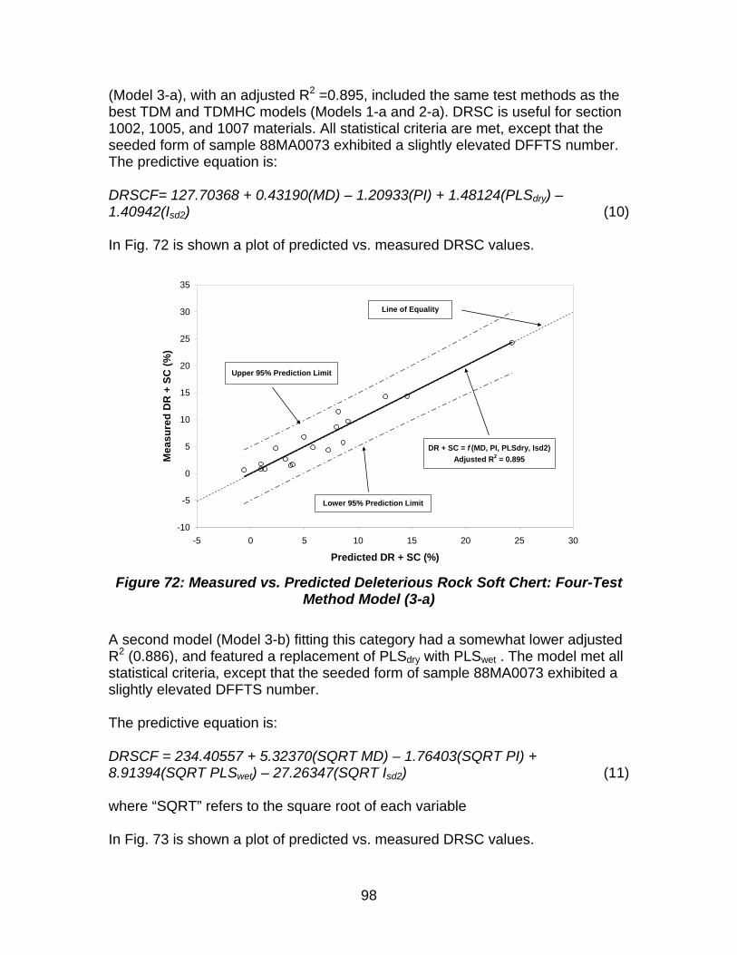
98

(Model 3-a), with an adjusted R2 =0.895, included the same test methods as the best TDM and TDMHC models (Models 1-a and 2-a). DRSC is useful for section 1002, 1005, and 1007 materials. All statistical criteria are met, except that the seeded form of sample 88MA0073 exhibited a slightly elevated DFFTS number. The predictive equation is: DRSCF= 127.70368 + 0.43190(MD) – 1.20933(PI) + 1.48124(PLSdry) – 1.40942(Isd2) (10) In Fig. 72 is shown a plot of predicted vs. measured DRSC values.

-10

-5

0

5

10

15

20

25

30

35

-5 0 5 10 15 20 25 30

Predicted DR + SC (%)

Mea

sure

d D

R +

SC

(%

)

DR + SC = f (MD, PI, PLSdry, Isd2)

Adjusted R2 = 0.895



Line of Equality

Figure 72: Measured vs. Predicted Deleterious Rock Soft Chert: Four-Test

Method Model (3-a)

A second model (Model 3-b) fitting this category had a somewhat lower adjusted R2 (0.886), and featured a replacement of PLSdry with PLSwet . The model met all statistical criteria, except that the seeded form of sample 88MA0073 exhibited a slightly elevated DFFTS number. The predictive equation is: DRSCF = 234.40557 + 5.32370(SQRT MD) – 1.76403(SQRT PI) + 8.91394(SQRT PLSwet) – 27.26347(SQRT Isd2) (11) where “SQRT” refers to the square root of each variable In Fig. 73 is shown a plot of predicted vs. measured DRSC values.

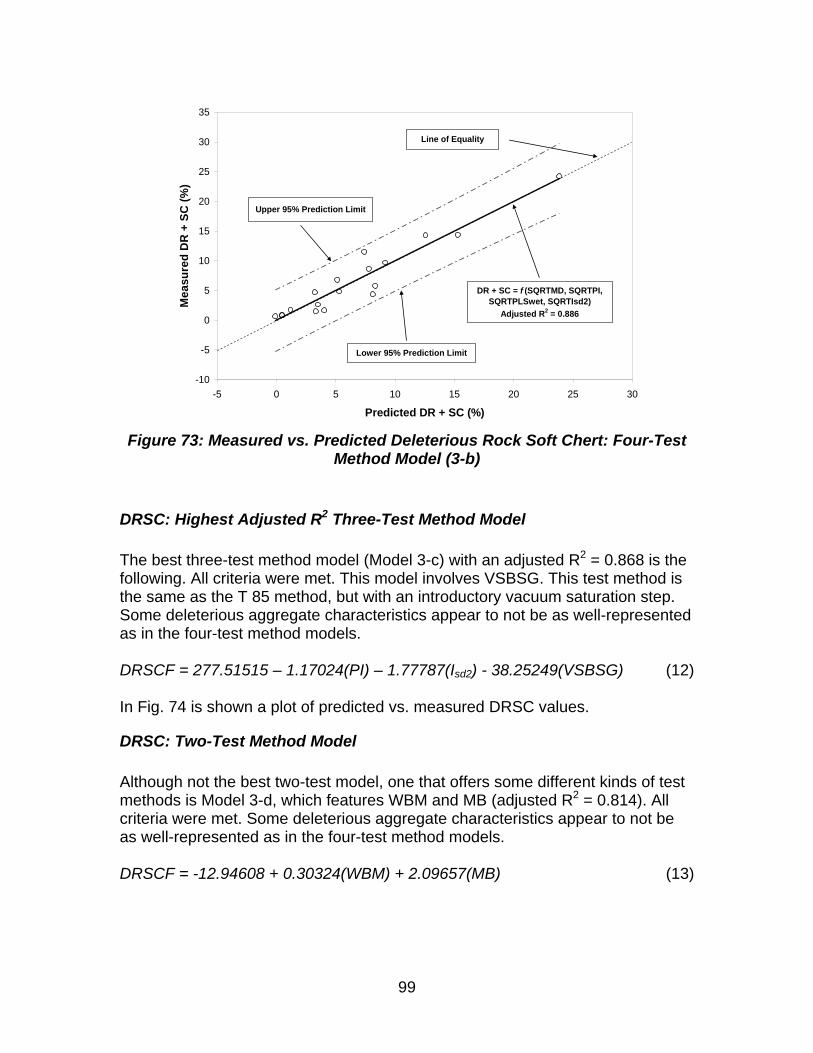
99

-10

-5

0

5

10

15

20

25

30

35

-5 0 5 10 15 20 25 30


Mea

sure

d D

R +

SC

(%

)

DR + SC = f (SQRTMD, SQRTPI, SQRTPLSwet, SQRTIsd2)

Adjusted R2 = 0.886



Line of Equality

Figure 73: Measured vs. Predicted Deleterious Rock Soft Chert: Four-Test

Method Model (3-b)

DRSC: Highest Adjusted R2 Three-Test Method Model

The best three-test method model (Model 3-c) with an adjusted R2 = 0.868 is the following. All criteria were met. This model involves VSBSG. This test method is the same as the T 85 method, but with an introductory vacuum saturation step. Some deleterious aggregate characteristics appear to not be as well-represented as in the four-test method models. DRSCF = 277.51515 – 1.17024(PI) – 1.77787(Isd2) - 38.25249(VSBSG) (12) In Fig. 74 is shown a plot of predicted vs. measured DRSC values.

DRSC: Two-Test Method Model

Although not the best two-test model, one that offers some different kinds of test methods is Model 3-d, which features WBM and MB (adjusted R2 = 0.814). All criteria were met. Some deleterious aggregate characteristics appear to not be as well-represented as in the four-test method models. DRSCF = -12.94608 + 0.30324(WBM) + 2.09657(MB) (13)

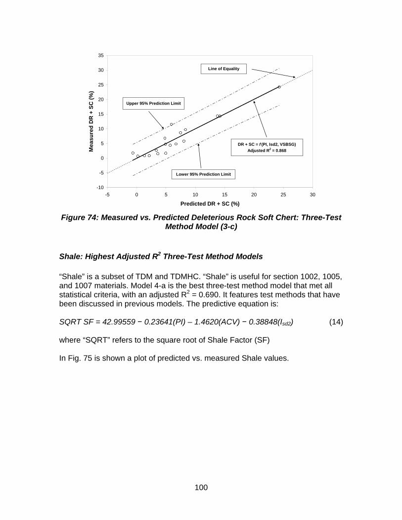
100

-10

-5

0

5

10

15

20

25

30

35

-5 0 5 10 15 20 25 30


Mea

sure

d D

R +

SC

(%

)

DR + SC = f (PI, Isd2, VSBSG)

Adjusted R2 = 0.868



Line of Equality

Figure 74: Measured vs. Predicted Deleterious Rock Soft Chert: Three-Test

Method Model (3-c)

Shale: Highest Adjusted R2 Three-Test Method Models

“Shale” is a subset of TDM and TDMHC. “Shale” is useful for section 1002, 1005, and 1007 materials. Model 4-a is the best three-test method model that met all statistical criteria, with an adjusted R2 = 0.690. It features test methods that have been discussed in previous models. The predictive equation is: SQRT SF = 42.99559 − 0.23641(PI) – 1.4620(ACV) − 0.38848(Isd2) (14) where “SQRT” refers to the square root of Shale Factor (SF) In Fig. 75 is shown a plot of predicted vs. measured Shale values.

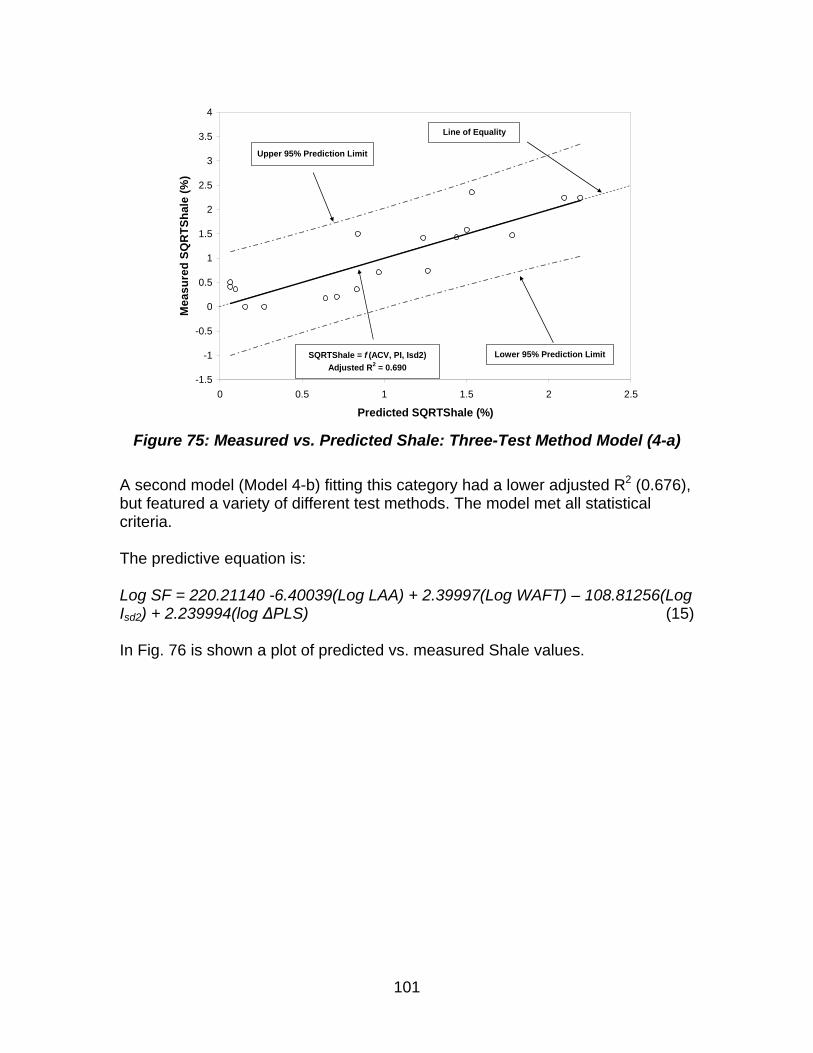
101

-1.5

-1

-0.5

0

0.5

1

1.5

2

2.5

3

3.5

4

0 0.5 1 1.5 2 2.5

Predicted SQRTShale (%)

Mea

sure

d S

QR

TS

hal

e (%

)

SQRTShale = f (ACV, PI, Isd2)

Adjusted R2 = 0.690



Line of Equality

Figure 75: Measured vs. Predicted Shale: Three-Test Method Model (4-a)

A second model (Model 4-b) fitting this category had a lower adjusted R2 (0.676), but featured a variety of different test methods. The model met all statistical criteria. The predictive equation is: Log SF = 220.21140 -6.40039(Log LAA) + 2.39997(Log WAFT) – 108.81256(Log Isd2) + 2.239994(log ΔPLS) (15) In Fig. 76 is shown a plot of predicted vs. measured Shale values.

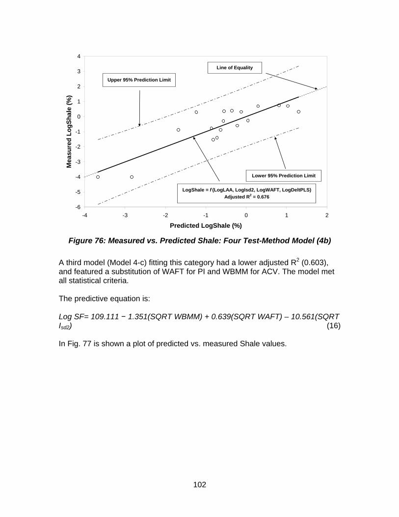
102

-6

-5

-4

-3

-2

-1

0

1

2

3

4

-4 -3 -2 -1 0 1 2

Predicted LogShale (%)

Mea

sure

d L

og

Sh

ale

(%

)

LogShale = f (LogLAA, LogIsd2, LogWAFT, LogDeltPLS)

Adjusted R2 = 0.676



Line of Equality

Figure 76: Measured vs. Predicted Shale: Four Test-Method Model (4b)

A third model (Model 4-c) fitting this category had a lower adjusted R2 (0.603), and featured a substitution of WAFT for PI and WBMM for ACV. The model met all statistical criteria. The predictive equation is: Log SF= 109.111 − 1.351(SQRT WBMM) + 0.639(SQRT WAFT) – 10.561(SQRT Isd2) (16) In Fig. 77 is shown a plot of predicted vs. measured Shale values.

103

-6

-5

-4

-3

-2

-1

0

1

2

3

4

-3.5 -3 -2.5 -2 -1.5 -1 -0.5 0 0.5 1 1.5

Predicted Log Shale (%)

Mea

sure

d L

og

Sh

ale (

%)

LShale = f (SQRTWBBM, SQRTIsd2, SQRTWAFT)

Adjusted R2 = 0.603



Line of Equality

Figure 77: Measured vs. Predicted Shale: Three-Test Method Model (4-c)

Estimation of Hard Chert Using TM-71 results, hard chert could be calculated by subtracting TDM from TDMHC (HC = TDMHC – TDM). To estimate HC, the same principal applies: HCF = TDMHCF – TDMF. The HCF could also be calculated from the individual material predictions: HCF = TDMHCF - [DRSCF + SF). It is somewhat more accurate to calculate HCF using the first method. Again, the inclusion of “F” in a term denotes a predicted or estimated value from a model; exclusion of “F” denotes aTM-71 Test result.

Estimation of TDM

Using TM-71 results (in the absence of OFM), TDM can be calculated by summing the subsets of TDM: TDM = DRSC + Shale. To estimate TDM, the same principal applies: TDMF = DRSCF + SF. The TDMF could also be calculated directly from the regression equation for TDMF. It is slightly more accurate to calculate TDMF using the first method.

Estimation of TDMHC Using TM-71 results (in the absence of OFM), TDMHC can be calculated by summing the subsets of TDMHC: TDMHC = DRSC + Shale + HC. To estimate TDMHC, the same principal applies: TDMHCF = DRSCF + SF + [TDMHCF – TDMF]. The TDMF could also be calculated directly from the regression equation for TDMHCF. It is very slightly more accurate to calculate TDMFHC using the second method.

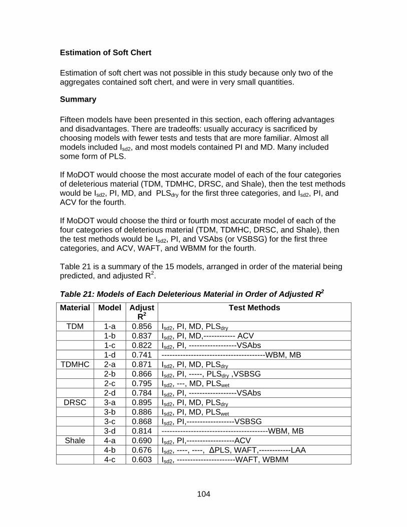
104

Estimation of Soft Chert

Estimation of soft chert was not possible in this study because only two of the aggregates contained soft chert, and were in very small quantities.

Summary

Fifteen models have been presented in this section, each offering advantages and disadvantages. There are tradeoffs: usually accuracy is sacrificed by choosing models with fewer tests and tests that are more familiar. Almost all models included Isd2, and most models contained PI and MD. Many included some form of PLS. If MoDOT would choose the most accurate model of each of the four categories of deleterious material (TDM, TDMHC, DRSC, and Shale), then the test methods would be Isd2, PI, MD, and PLSdry for the first three categories, and Isd2, PI, and ACV for the fourth. If MoDOT would choose the third or fourth most accurate model of each of the four categories of deleterious material (TDM, TDMHC, DRSC, and Shale), then the test methods would be Isd2, PI, and VSAbs (or VSBSG) for the first three categories, and ACV, WAFT, and WBMM for the fourth. Table 21 is a summary of the 15 models, arranged in order of the material being predicted, and adjusted R2. Table 21: Models of Each Deleterious Material in Order of Adjusted R2

Material Model Adjust R2

Test Methods

TDM 1-a 0.856 Isd2, PI, MD, PLSdry 1-b 0.837 Isd2, PI, MD,------------ ACV 1-c 0.822 Isd2, PI, ------------------VSAbs 1-d 0.741 ---------------------------------------WBM, MB

TDMHC 2-a 0.871 Isd2, PI, MD, PLSdry 2-b 0.866 Isd2, PI, -----, PLSdry ,VSBSG 2-c 0.795 Isd2, ---, MD, PLSwet 2-d 0.784 Isd2, PI, ------------------VSAbs

DRSC 3-a 0.895 Isd2, PI, MD, PLSdry 3-b 0.886 Isd2, PI, MD, PLSwet 3-c 0.868 Isd2, PI,------------------VSBSG 3-d 0.814 ----------------------------------------WBM, MB

Shale 4-a 0.690 Isd2, PI,------------------ACV 4-b 0.676 Isd2, ----, ----, ΔPLS, WAFT,------------LAA 4-c 0.603 Isd2, ----------------------WAFT, WBMM

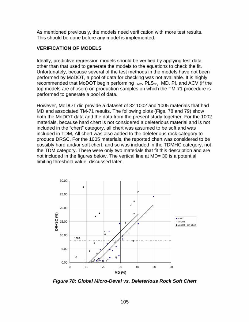
105

As mentioned previously, the models need verification with more test results. This should be done before any model is implemented.

VERIFICATION OF MODELS Ideally, predictive regression models should be verified by applying test data other than that used to generate the models to the equations to check the fit. Unfortunately, because several of the test methods in the models have not been performed by MoDOT, a pool of data for checking was not available. It is highly recommended that MoDOT begin performing Isd2, PLSdry, MD, PI, and ACV (if the top models are chosen) on production samples on which the TM-71 procedure is performed to generate a pool of data. However, MoDOT did provide a dataset of 32 1002 and 1005 materials that had MD and associated TM-71 results. The following plots (Figs. 78 and 79) show both the MoDOT data and the data from the present study together. For the 1002 materials, because hard chert is not considered a deleterious material and is not included in the “chert” category, all chert was assumed to be soft and was included in TDM, All chert was also added to the deleterious rock category to produce DRSC. For the 1005 materials, the reported chert was considered to be possibly hard and/or soft chert, and so was included in the TDMHC category, not the TDM category. There were only two materials that fit this description and are not included in the figures below. The vertical line at MD= 30 is a potential limiting threshold value, discussed later.

0.00

5.00

10.00

15.00

20.00

25.00

30.00

0 10 20 30 40 50 60

MD (%)

DR

+S

C (

%)

MS&T

MoDOT

MoDOT High Chert

1002

Figure 78: Global Micro-Deval vs. Deleterious Rock Soft Chert

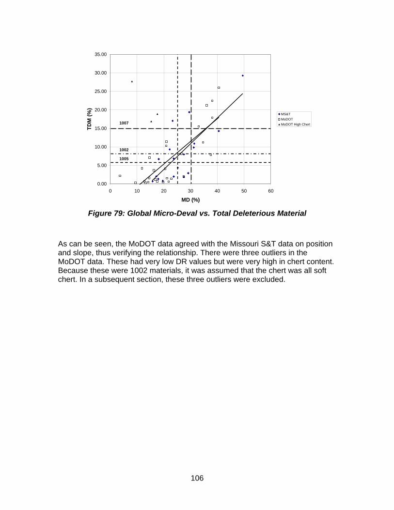
106

0.00

5.00

10.00

15.00

20.00

25.00

30.00

35.00

0 10 20 30 40 50 60

MD (%)

TD

M (

%)

MS&T

MoDOT

MoDOT High Chert

1005

1002

1007

Figure 79: Global Micro-Deval vs. Total Deleterious Material

As can be seen, the MoDOT data agreed with the Missouri S&T data on position and slope, thus verifying the relationship. There were three outliers in the MoDOT data. These had very low DR values but were very high in chert content. Because these were 1002 materials, it was assumed that the chert was all soft chert. In a subsequent section, these three outliers were excluded.

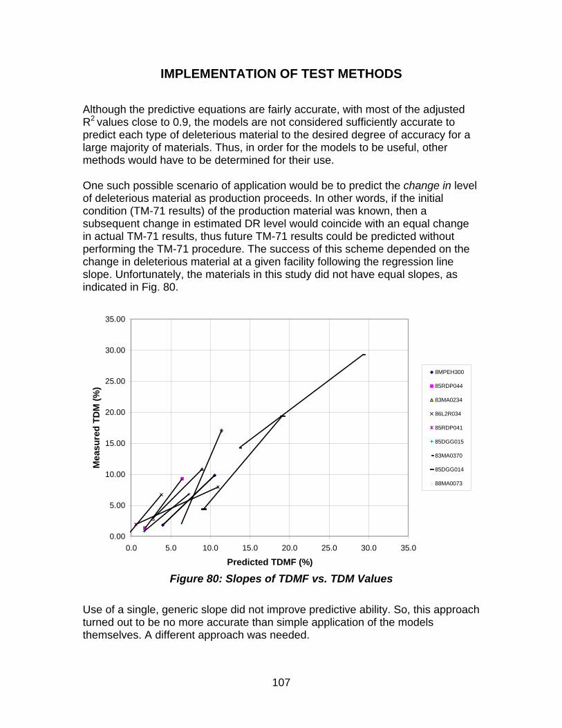
107

IMPLEMENTATION OF TEST METHODS

Although the predictive equations are fairly accurate, with most of the adjusted R2 values close to 0.9, the models are not considered sufficiently accurate to predict each type of deleterious material to the desired degree of accuracy for a large majority of materials. Thus, in order for the models to be useful, other methods would have to be determined for their use. One such possible scenario of application would be to predict the change in level of deleterious material as production proceeds. In other words, if the initial condition (TM-71 results) of the production material was known, then a subsequent change in estimated DR level would coincide with an equal change in actual TM-71 results, thus future TM-71 results could be predicted without performing the TM-71 procedure. The success of this scheme depended on the change in deleterious material at a given facility following the regression line slope. Unfortunately, the materials in this study did not have equal slopes, as indicated in Fig. 80.

0.00

5.00

10.00

15.00

20.00

25.00

30.00

35.00

0.0 5.0 10.0 15.0 20.0 25.0 30.0 35.0

Predicted TDMF (%)

Mea

sure

d T

DM

(%

)

8MPEH300

85RDP044

83MA0234

86L2R034

85RDP041

85DGG015

83MA0370

85DGG014

88MA0073

Figure 80: Slopes of TDMF vs. TDM Values

Use of a single, generic slope did not improve predictive ability. So, this approach turned out to be no more accurate than simple application of the models themselves. A different approach was needed.

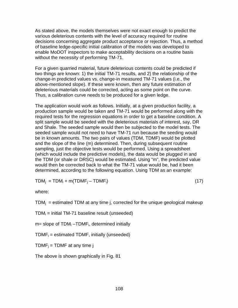
108

As stated above, the models themselves were not exact enough to predict the various deleterious contents with the level of accuracy required for routine decisions concerning aggregate product acceptance or rejection. Thus, a method of baseline ledge-specific initial calibration of the models was developed to enable MoDOT inspectors to make acceptability decisions on a routine basis without the necessity of performing TM-71. For a given quarried material, future deleterious contents could be predicted if two things are known: 1) the initial TM-71 results, and 2) the relationship of the change-in predicted values vs. change-in measured TM-71 values (i.e., the above-mentioned slope). If these were known, then any future estimation of deleterious materials could be corrected, acting as some point on the curve. Thus, a calibration curve needs to be produced for a given ledge. The application would work as follows. Initially, at a given production facility, a production sample would be taken and TM-71 would be performed along with the required tests for the regression equations in order to get a baseline condition. A split sample would be seeded with the deleterious materials of interest, say, DR and Shale. The seeded sample would then be subjected to the model tests. The seeded sample would not need to have TM-71 run because the seeding would be in known amounts. The two pairs of values (TDM, TDMF) would be plotted and the slope of the line (m) determined. Then, during subsequent routine sampling, just the objective tests would be performed. Using a spreadsheet (which would include the predictive models), the data would be plugged in and the TDM (or shale or DRSC) would be estimated. Using “m”, the predicted value would then be corrected back to what the TM-71 value would be, had it been determined, according to the following equation. Using TDM as an example: TDMj = TDMi + m(TDMFj – TDMFi) (17) where: TDMj = estimated TDM at any time j, corrected for the unique geological makeup TDMi = initial TM-71 baseline result (unseeded) m= slope of TDMi –TDMFi, determined initially TDMFi = estimated TDMF, initially (unseeded) TDMFj = TDMF at any time j The above is shown graphically in Fig. 81

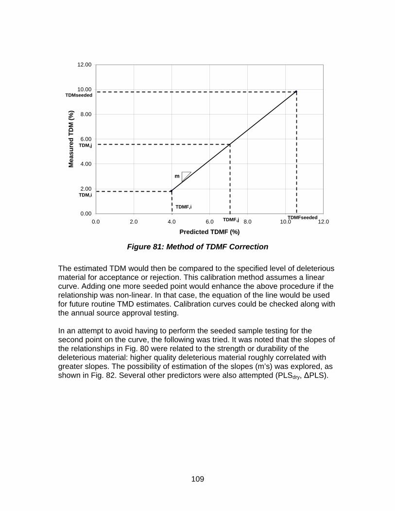
109

0.00

2.00

4.00

6.00

8.00

10.00

12.00

0.0 2.0 4.0 6.0 8.0 10.0 12.0

Predicted TDMF (%)

Me

as

ure

d T

DM

(%

)

TDMF,j

TDMF,i

TDM,j

TDM,i

m

TDMFseeded

TDMseeded

Figure 81: Method of TDMF Correction

The estimated TDM would then be compared to the specified level of deleterious material for acceptance or rejection. This calibration method assumes a linear curve. Adding one more seeded point would enhance the above procedure if the relationship was non-linear. In that case, the equation of the line would be used for future routine TMD estimates. Calibration curves could be checked along with the annual source approval testing. In an attempt to avoid having to perform the seeded sample testing for the second point on the curve, the following was tried. It was noted that the slopes of the relationships in Fig. 80 were related to the strength or durability of the deleterious material: higher quality deleterious material roughly correlated with greater slopes. The possibility of estimation of the slopes (m’s) was explored, as shown in Fig. 82. Several other predictors were also attempted (PLSdry, ΔPLS).

110

0.00

0.50

1.00

1.50

2.00

2.50

3.00

3.50

0 0.5 1 1.5 2 2.5 3

PLSwet, MPa

Slo

pe

Figure 82: Estimation of Slope “m” by PLSwet

However, as can be seen, although there is a relationship between PLSwet and slope “m”, it is not strong enough to accurately be substituted for the actual determination of the slope “m” for a given deleterious material. Thus, the calibration curve will have to be created. MoDOT employs a similar scenario for determination of the air content of paving concrete. The desired location of air content sampling is behind the paver, but it is more convenient to sample in front of the paver. To allow before-paver sampling yet estimate behind-paver results, samples are initially taken at both locations and the difference between the two values is used as a calibration factor to be applied to subsequent, routine before-paver test results. At present, MoDOT performs the MD, T 85 BSG, PI, and the TM-71 test methods at the district and the Central Laboratory facilities. TM-71 and PI are also performed at production facilities. Isd2, PLS, and ACV are not currently being done by MoDOT. Whether routine production samples can be taken to district laboratories or must be performed on-site at quarries and plants will have to be decided upon by MoDOT. The Isd2, PLS, and ACV test methods are fairly simple and will require minimal training. Equipment installation and space requirements are nominal. Current costs for the required devices are as follows:

111

1) MD: single container = $2400, dual container = $4600, triple container =

$5205 2) Slake Durability: dual drum = $3680, four drum = $5080 3) PLS: $3558 4) ACV: mold = $90; use concrete compression machine if available

Total elapsed time for the objective tests in the models is nominally two to three days, if the 24 hr drying times are adhered to. However, experience has shown that many times, granular materials can be dried more quickly. To make the system more practical, MoDOT would have to determine if shorter drying times could be used, thus reducing the overall test method durations.

FLOWCHART ACCEPTANCE

Threshold Limit Development

Another approach, besides prediction of deleterious materials by regression, is to create a system of threshold limits for several key test method results. Thus, if a given sample exhibits values that exceed any of the test method threshold limits, the probability of its TDM, DRSC, and Shale contents being acceptable would be low. It was not originally anticipated that this sort of system would be feasible because of concern that some parent materials may have test values that would fail a threshold system by themselves, with little or no deleterious material present. However, preliminary data from MoDOT indicates that the threshold system method may have promise. The test methods that were considered for a threshold system were limited to the ones included in the best models plus several more that were in lesser models. Also, T 85 BSG and Abs were considered because they are highly correlated with their vacuum saturated counterparts, and in fact, the limited dataset in this study showed no statistical difference between the methods. The data used for setting the limits included the nine materials (and their seeded counterparts) in this study, plus an additional dataset of 29 materials made available by MoDOT. However, the MoDOT data was limited to LAA, MD, WAFT, and NaSO4. Only TDM was explored in this analysis because this is just a demonstration of what could be done when more data becomes available. Table 22 shows the example threshold limits for 1002, 1005, and 1007 materials. Plots of various test method results against TDM helped delineate where the limits should fall.

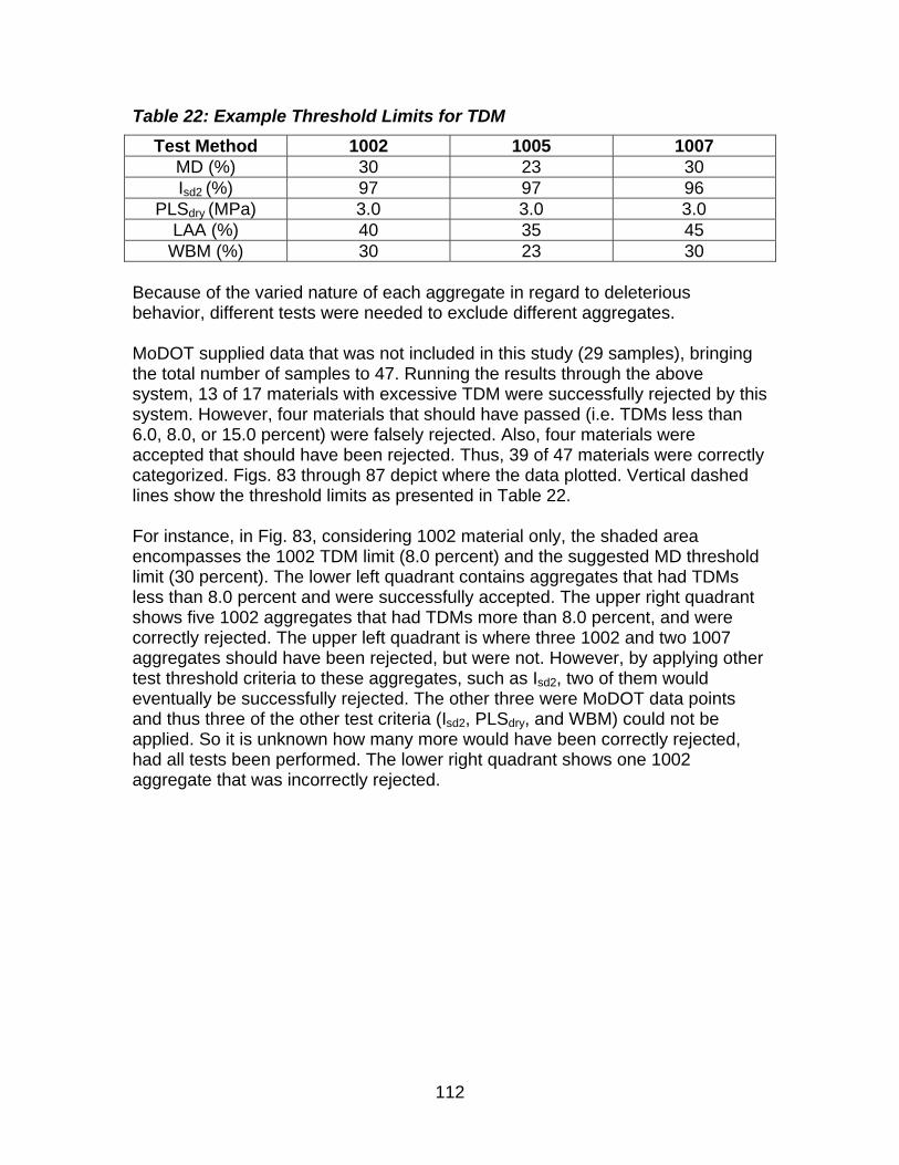
112

Table 22: Example Threshold Limits for TDM

Test Method 1002 1005 1007 MD (%) 30 23 30 Isd2 (%) 97 97 96

PLSdry (MPa) 3.0 3.0 3.0 LAA (%) 40 35 45

WBM (%) 30 23 30 Because of the varied nature of each aggregate in regard to deleterious behavior, different tests were needed to exclude different aggregates. MoDOT supplied data that was not included in this study (29 samples), bringing the total number of samples to 47. Running the results through the above system, 13 of 17 materials with excessive TDM were successfully rejected by this system. However, four materials that should have passed (i.e. TDMs less than 6.0, 8.0, or 15.0 percent) were falsely rejected. Also, four materials were accepted that should have been rejected. Thus, 39 of 47 materials were correctly categorized. Figs. 83 through 87 depict where the data plotted. Vertical dashed lines show the threshold limits as presented in Table 22. For instance, in Fig. 83, considering 1002 material only, the shaded area encompasses the 1002 TDM limit (8.0 percent) and the suggested MD threshold limit (30 percent). The lower left quadrant contains aggregates that had TDMs less than 8.0 percent and were successfully accepted. The upper right quadrant shows five 1002 aggregates that had TDMs more than 8.0 percent, and were correctly rejected. The upper left quadrant is where three 1002 and two 1007 aggregates should have been rejected, but were not. However, by applying other test threshold criteria to these aggregates, such as Isd2, two of them would eventually be successfully rejected. The other three were MoDOT data points and thus three of the other test criteria (Isd2, PLSdry, and WBM) could not be applied. So it is unknown how many more would have been correctly rejected, had all tests been performed. The lower right quadrant shows one 1002 aggregate that was incorrectly rejected.

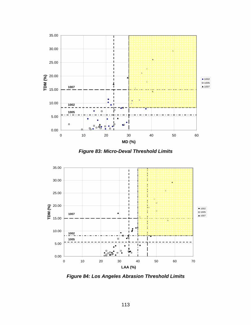
113

0.00

5.00

10.00

15.00

20.00

25.00

30.00

35.00

0 10 20 30 40 50 60

MD (%)

TD

M (

%)

1002

1005

1007

1005

1002

1007

Figure 83: Micro-Deval Threshold Limits

0.00

5.00

10.00

15.00

20.00

25.00

30.00

35.00

0 10 20 30 40 50 60 70

LAA (%)

TD

M (

%)

1002

1005

1007

1005

1002

1007

Figure 84: Los Angeles Abrasion Threshold Limits

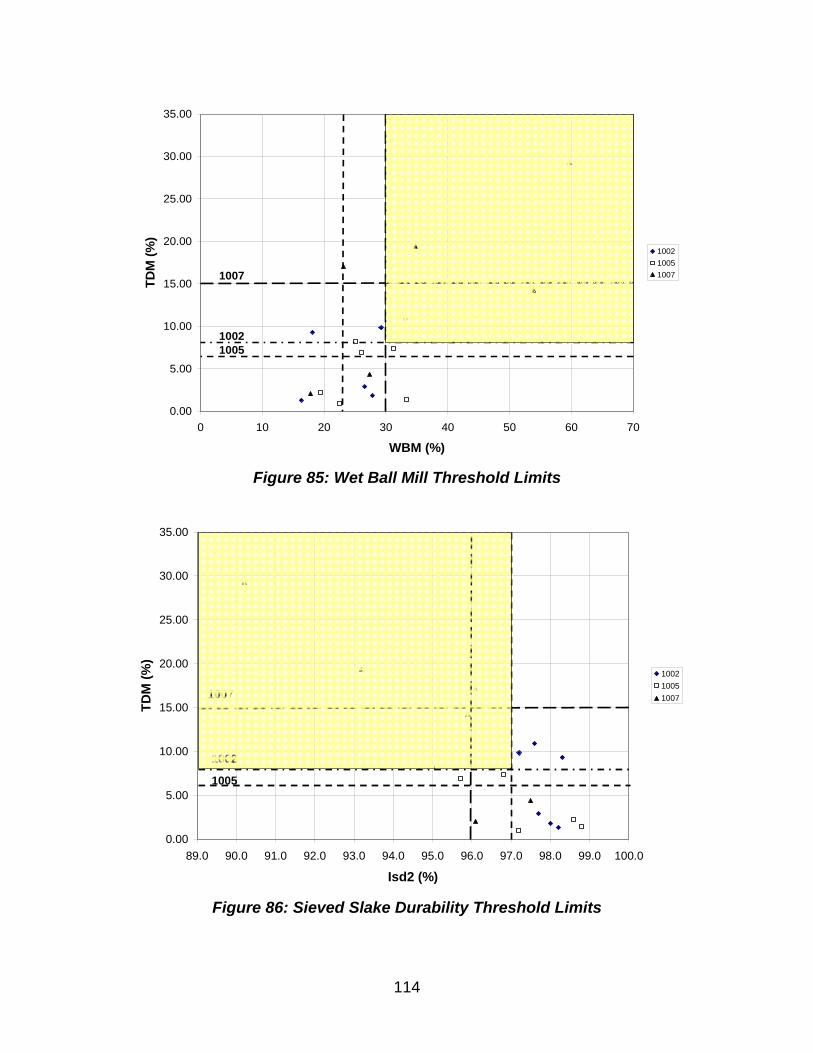
114

0.00

5.00

10.00

15.00

20.00

25.00

30.00

35.00

0 10 20 30 40 50 60 70

WBM (%)

TD

M (

%)

1002

1005

1007

10051002

1007

Figure 85: Wet Ball Mill Threshold Limits

0.00

5.00

10.00

15.00

20.00

25.00

30.00

35.00

89.0 90.0 91.0 92.0 93.0 94.0 95.0 96.0 97.0 98.0 99.0 100.0

Isd2 (%)

TD

M (

%)

1002

1005

1007

1005

1002

1007

Figure 86: Sieved Slake Durability Threshold Limits

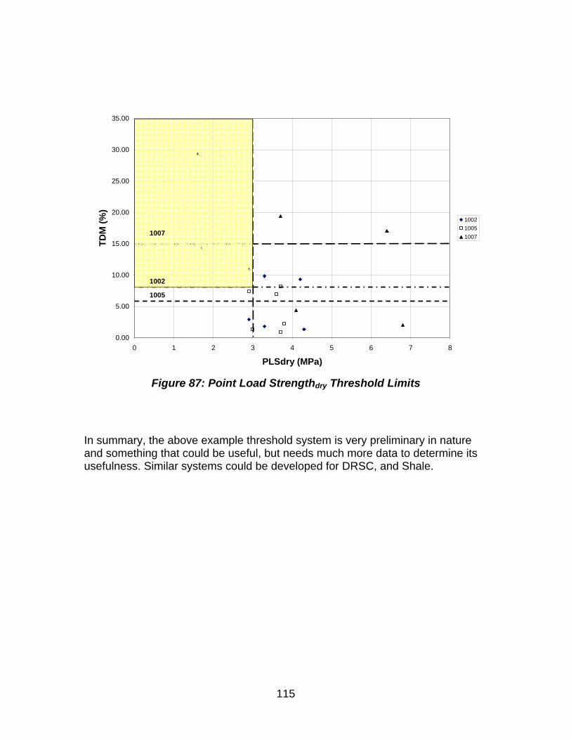
115

0.00

5.00

10.00

15.00

20.00

25.00

30.00

35.00

0 1 2 3 4 5 6 7 8

PLSdry (MPa)

TD

M (

%)

1002

1005

1007

1005

1002

1007

Figure 87: Point Load Strengthdry Threshold Limits

In summary, the above example threshold system is very preliminary in nature and something that could be useful, but needs much more data to determine its usefulness. Similar systems could be developed for DRSC, and Shale.

116

CONCLUSIONS

Fifteen regression models have been developed to predict various deleterious material contents of aggregates specified in MoDOT’s standard specifications sections 1002, 1005, and 1007. Four models predict total deleterious materials (TDM) (sections 1002 and 1007), four predict total deleterious materials including hard chert (TDMHC) (section 1005), four predict deleterious rock plus soft chert (DRSC), a subset of both TDM and TDMHC, and three predict shale, a subset of both TDM and TDMHC. Hard chert can be back-calculated from TDMF and TDMHCF values. Within a given type of deleterious material, the choice of model depends on the factors like desired ease of testing, familiarity with test methods, equipment cost, sensitivity to test duration, and level of accuracy that is considered acceptable. There is a trade-off between accuracy of prediction and the above-listed factors. All models contained some test methods for which MoDOT has no historical data, thus, verification of the models was not possible. Therefore, the models should be considered preliminary until proven.

TOTAL DELETERIOUS MATERIALS (TDM) MODELS The most accurate TDM model [Model 1-a] (adjusted R2 = 0.856) entailed two tests performed routinely by MoDOT (MD and PI), and two tests that are not currently being performed (PLSdry and Isd2). The PLSdry was also recommended in a recent study for MoDOT that dealt with prediction of AASHTO T 161 results. The second-most accurate TDM model [Model 1-b] (adjusted R2 = 0.837) contained routine tests (PI and MD), and tests that are not currently being performed (ACV and Isd2). The third-most accurate TDM model [Model 1-c] (adjusted R2 = 0.822) was simpler: it contained a routine test (PI), and two tests that are not currently being performed (VSAbs and Isd2). The fourth-most accurate TDM model [Model 1-d] (adjusted R2 = 0.741) was fairly simple: it contained a test that MoDOT is currently evaluating (WBM), and a test that is not currently being performed (MB).

TOTAL DELETERIOUS MATERIALS HARD CHERT (TDMHC) MODELS The most accurate TDMHC model [Model 2-a] (adjusted R2 = 0.871) contained the same tests as the most accurate TDM model (MD, PI, PLSdry and Isd2). The second-most accurate TDMHC model [Model 2-b] (adjusted R2 = 0.866) contained a routine test (PI), and tests that are not currently being performed (VSBSG, PLSdry and Isd2).

117

The third-most accurate TDMHC model [Model 2-c] (adjusted R2 = 0.795) was the simplest: it contained a routine test (MD), and tests that are not currently being performed (PLSwet and Isd2). A fourth TDMHC model [Model 2-d] (adjusted R2 = 0.784) contained the same test methods as Model 1-c: PI, VSAbs and Isd2

HARD CHERT Hard chert content is estimated by calculating the difference between the predicted values of TDMHC and TDM.

DELETERIOUS ROCK SOFT CHERT (DRSC) MODELS

The most accurate DRSC model [Model 3-a] (adjusted R2 = 0.895) contained the same tests as the most accurate TDM model (MD, PI, PLSdry and Isd2). The second-most accurate DRSC model [Model 3-b] (adjusted R2 = 0.886) contained the same tests as the most accurate model (MD, PI, and Isd2) with the substitution of PLSwet for PLSdry. The third-most accurate DRSC model [Model 3-c] (adjusted R2 = 0.868) contained PI, VSBSG, and Isd2. The fourth-most accurate DRSC model [Model 3-d] (adjusted R2 = 0.814) contained WBM and MB.

SHALE MODELS

In regard to shale, the most accurate model [Model 4-a] (adjusted R2 = 0.690) contained PI, ACV, and Isd2.

The second-most accurate shale model [Model 4-b] (adjusted R2 = 0.676) contained ΔPLS, WAFT, LAA. and Isd2. The least accurate shale model [Model 4-c] (0.603) contained Isd2, WAFT, and WBMM. None of the Shale models are very accurate.

TEST METHODS MD was in all good models. This was not surprising, based on the literature review.

118

VSAbs gave greater values than T 85 Abs, but the results were not considered significant at the 0.05 α level in this limited study. LAA and ACV were highly correlated, as expected from the literature review. PI, SE, and MB did not correlate well with each other, as expected. However, it is suspected that if all three tests were performed on minus #200 materials and subjected to the same preparation, the correlations would improve. The WBMM modified version of the WBM test always had better correlations with the deleterious materials than the WBM. It seems that there is promise in improving the WBM.

MODEL STRATEGIES If MoDOT would choose the most accurate model of each of the four categories of deleterious material (TDM, TDMHC, DRSC, and Shale), then the test methods would be Isd2, PI, MD, and PLSdry for the first three categories, and Isd2, PI, and ACV for the fourth. If MoDOT would choose the third or fourth most accurate model of each of the four categories of deleterious material (TDM, TDMHC, DRSC, and Shale), then the test methods would be Isd2, PI, and VSAbs (or VSBSG) for the first three categories, and ACV, WAFT, and WBMM for the fourth. Testing time for all models is on the order of two to three days. However, the total interval could be shortened if it could be shown that drying times are too conservative. Although the use of the predictive system probably has a longer total duration time and may entail greater total technician time-on-task than the TM-71 method, the results should be much more objective and repeatable. The regression models themselves were not exact enough to predict the various deleterious contents with the level of accuracy required for routine decisions concerning aggregate product acceptance or rejection. Thus, a method of baseline ledge-specific initial calibration of the models was developed to enable MoDOT inspectors to make acceptability decisions on a routine basis without the necessity of performing TM-71. The precision of TM-71 has not been reported, thus a comparison of the models prediction to TM-71 precision could not be made. Once the models are chosen, MoDOT should begin generating test data. After a significant amount of data is accumulated, the models need to be checked and then modified.

119

THRESHOLD LIMITS

A second system of evaluation entailed the use of a set of threshold limits set on various aggregate test method results. The test methods include LAA, WBM, MD, PLSdry and Isd2. The limits are to be considered preliminary until proven with a larger data set. More thresholds based on other test methods may appear.

120

RECOMMENDATIONS – FUTURE RESEARCH

Future research should include verification, or even extension, of the models by performing additional tests to obtain the necessary data. As a start, models 1-a, 2-a, and 3-a, can be verified by performing PI, Isd2 and PLSdry tests on the 29 member data set used in this study in the Threshold Limits section. Additionally, by performing ACV, model 4-a can be checked. At any point, the regressions can be run again with a larger data set. And, the threshold system can be fine-tuned by moving the limits to balance acceptance and rejection. The calibration procedure should also be verified by seeding production samples, performing TM-71 and model tests on the seeded and unseeded splits, then using the calibration curves for subsequent testing. The WBM procedure has promise, and needs fine-tuning by standardizing such variables as matching the number of balls to the NMS (like LAA), the number of revolutions, and standard gradations like LAA or MD. Results of PI, SE, and MB should agree more than they do. Future research should entail performing all these tests on minus #200 material to help reduce the influence of gradation. At that point, MB may emerge as the method of choice for future modifications of the regression models.

121

GLOSSARY

AASHTO= American Association of State Highway and Transportation Officials Abs= T 85 absorption ACV= aggregate crushing value Adj R2= adjusted R2 ASTM= American Society of Testing and Materials BSG= T 85 bulk specific gravity (dry) CArE= Civil, Architectural, and Environmental Engineering CN= Condition Number CTE= coefficient of thermal expansion CV= coefficient of variation DF= T161 Durability Factor DFFITS= difference of fits DR= deleterious rock DRSC= deleterious rock plus soft chert DRSCF= deleterious rock plus soft chert factor HC= hard chert HCF= hard chert factor HWTD= Hamburg Wheel Tracking Device Isd2= sieved slake durability ISSA= International Slurry Seal Association LAA= Los Angeles Abrasion MAS= maximum aggregate size MB= methylene blue MD= micro-Deval MoDOT= Missouri Department of Transportation NaSO4= sodium sulfate soundness NMS= nominal maximum size PLS= point load strength QC= quality control R= correlation coefficient R2= coefficient of determination SC= soft chert SF= shale factor SSD= saturated, surface dry TDM= total deleterious material TDMF= total deleterious material factor TDMHC= total deleterious material plus hard chert TDMHCF= total deleterious material plus hard chert factor VIF= Variance Inflation Factor VSAbs= vacuum saturated absorption VSBSG= vacuum saturated bulk specific gravity (dry) WAFT= water alcohol freeze thaw WBM= wet ball mill WBMM= wet ball mill modified

122

REFERENCES

American Association of State Highway and Transportation Officials (AASHTO). (1999). “Standard Specification for Mineral Filler for Bituminous Paving Mixtures.” M 17-99, Washington, D.C. American Association of State Highway and Transportation Officials (AASHTO). (1999). “Standard Specification for Coarse Aggregate for Portland Cement Concrete.” M 80-99, Washington, D.C. American Association of State Highway and Transportation Officials (AASHTO). (2000). “Standard Method of Test for Resistance of Concrete to Rapid Freezing and Thawing.” T 161-00, Washington, D.C. American Association of State Highway and Transportation Officials (AASHTO). (2007). “Standard Method of Test for Soundness of Aggregates by Freezing and Thawing.” T 103-07, Washington, D.C. American Association of State Highway and Transportation Officials (AASHTO). (2000). “Standard Method of Test for Specific Gravity and Absorption of Coarse Aggregate.” T 85-00, Washington, D.C. American Association of State Highway and Transportation Officials (AASHTO). (2002). “Standard Method of Test for Resistance to Degradation of Small-Size Coarse Aggregate by Abrasion and Impact in the Los Angeles Machine.” T 96-02, Washington, D.C. American Association of State Highway and Transportation Officials (AASHTO). (2006). “Standard Method of Test for Resistance of Coarse Aggregate to Degradation by Abrasion in the Micro-Deval Apparatus.” T 327-06, Washington, D.C. American Association of State Highway and Transportation Officials (AASHTO). (2003). “Standard Method of Test for Soundness of Aggregate by Use of Sodium Sulfate or Magnesium Sulfate.” T 104-03, Washington, D.C. American Association of State Highway and Transportation Officials (AASHTO). (2007). “Standard Method of Test for Methylene Blue Value of Clays, Mineral Fillers, and Fines.” T 330-07, Washington, D.C. American Association of State Highway and Transportation Officials (AASHTO). (2005). “Standard Method of Test for Theoretical Maximum Specific Gravity and Density of Asphalt Paving Mixtures.” T 209-05, Washington, D.C.

123

American Association of State Highway and Transportation Officials (AASHTO). (2000). “Standard Method of Test for Clay Lumps and Friable Particles in Aggregate.” T 112-00, Washington, D.C. American Association of State Highway and Transportation Officials (AASHTO). (2002). “Standard Method of Test for Lightweight Pieces in Aggregate.” T 113-02, Washington, D.C. American Association of State Highway and Transportation Officials (AASHTO). (2000). “Standard Method of Test for Materials Finer than 75- μm (No. 200) Sieve in Mineral Aggregates by Washing.” T 11-00. Washington, D.C. American Association of State Highway and Transportation Officials (AASHTO). (2003). “Standard Method of Test for Resistance of Compacted Asphalt Mixtures to Moisture-Induced Damage.” T 283-03. Washington, D.C. American Association of State Highway and Transportation Officials (AASHTO). (2002). “Standard Test Method for Plastic Fines in Graded Aggregates and Soils by Use of the Sand Equivalent Test.” T 176-02, Washington, D.C. American Association of State Highway and Transportation Officials (AASHTO). (2000). “Standard Test Method for Determining the Plastic Limit and Plasticity Index of Soils.” T 90-00, Washington, D.C. American Association of State Highway and Transportation Officials (AASHTO). (2002). “Standard Test Method for Determining the Liquid Limit of Soils.” T 89-02, Washington, D.C. American Society of Testing and Materials (ASTM). (2007). “Standard Test Method Determination of the Point Load Strength Index of Rock and Application to Rock Strength Classifications.” D 5731-07, Philadelphia, Pennsylvania. American Society of Testing and Materials (ASTM). (2008). “Standard Practice for Dealing with Outlying Observations.” E 178-08, Philadelphia, Pennsylvania. American Society of Testing and Materials (ASTM). (2007). “Standard Specification for Fine Aggregate in Bituminous Paving Mixtures.” D 1073-07, Philadelphia. American Society of Testing and Materials (ASTM). (2009). “Standard Specification for Mineral Filler for Bituminous Paving Mixtures.” D 242-09, Philadelphia, Pennsylvania. American Society for Testing and Materials (ASTM). (2004). “Standard Test Method for Slake Durability of Shales and Similar Weak Rocks.” D 4644-04, Philadelphia, Pennsylvania.

124

American Society for Testing and Materials(ASTM). (2002). “Standard Test Method for Sand Equivalent Values of Soil and Fine Aggregate.” D 2419-02, Philadelphia, Pennsylvania. Aschenbrener, T. (1992). “Comparison of Colorado Component Hot Mix Asphalt Materials with Some European Specifications.” Research Report CDOT-DTD-R-92-14. Colorado Dept. of Transportation, Denver, Colorado, 65. Aschenbrener, T., and Zamora, R. (1995). “Evaluation of Specialized Tests for Aggregates Used in Hot Mix Asphalt Pavements in Colorado.” Transportation Research Record. 1486, Transportation Research Board, Washington, D.C., 130-136. Bieniawski, Z.T. (1975). “The Point-Load Test in Geotechnical Practice.” Engineering Geology. 9, Amsterdam, 1-11. Bjarnason, G., Petursson, P., and Erlingsson, S. (2000). “Aggregates Resistance to Fragmentation, Weathering, and Abrasion.” Unbound Aggregates in Road Construction, A.R. Dawson, ed, 3-11. Bloem, D.L. (1966). “Soundness and Deleterious Substances.” Significance of Tests and Properties of Concrete and Concrete-Making Materials. STP 169a. American Society for Testing and Materials, Philadelphia, Pennsylvania, 497-512. Brink, R.H. (1958). “Rapid Tests for Aggregate and Concrete Presented at the Thirty-Seventh Annual Meeting.” National Research Council (U.S.), Highway Research Board, Washington, D.C. British Standards Institution. (BSI). (1990). “Methods for Determination of Aggregate Crushing Value (ACV).” BS 812: Part 110, London. British Standards Institution. (BSI). (1998). “Tests for Mechanical and Physical Properties of Aggregates. Methods for the Determination of Resistance to Fragmentation.” BS 1097: Part 2, London. Broch, E., and Franklin, J.A. (1972). “The Point-Load Test.” Int. Journal of Rock Mechanics Min. Science, 9, 664-697. Buth, E., Ivey, D. L., and Hirsch, T. J. (1964). “Correlation of Concrete Properties with Tests for Clay Content of Aggregate.” Texas Transportation Institute, Texas A & M University, College Station, Texas, 20.

125

Buth, E., Ivey, D. L., Hirsch, T. J. (1967). “Clay, Aggregate, and Concrete.” Research Report No. 71-3 (Final), Texas Transportation Institute, Texas A & M University, College Station, Texas. Cady, P.D. (1984). “Soundness Testing and Durability of Coarse Aggregates in Concrete.” Cement, Concrete, and Aggregate (CCAGDP). 6(1), 43-46. Chamberlain, W. (1981). “Aggregate Porosity and Concrete Freeze-Thaw Resistance.” FHWA/NY/SR-81/71, Washington, D.C. Clifton, A.W., Klassen, M.J., and Watters, B.R. (1987). “Production and Testing of Ballast.” Transportation Research Record. 1131, Transportation Research Board, Washington, D.C., 26-34. Clifton, A.W., M.J. Klassen, and Watters, B.R. (1987). “Track Evaluation and Ballast Performance Specifications,” Transportation Research Record. 1131, Transportation Research Board, Washington, D.C., 35-44. Clough, R.H., and Martinez, J.E. (1961). “Research on Bituminous Pavements Using the Sand Equivalent Test.” Highway Research Bulletin 300, Washington, D.C., 1-17. Cooley, J., and James, R.S. (2003). “Micro-Deval Testing of Aggregates in the Southeast.” Transportation Research Record, 1837, Washington, D.C., 73-79. Cordon, W.A. (1948). “Selection of Concrete Aggregates.” Lecture No. 4. U.S Bureau of Reclamation. Cross, S.A, and Voth, M.D. (2001). “Evaluation of Anti-Stripping Agents Using the Asphalt Pavement Analyzer.” Report No. K-TRAN: KU-99-3, Univ. of Kansas, Lawrence, Kansas, 110. Cuelho, E., Mokwa, R., and Obert, K. (2007). “Comparative Analysis of Coarse Surfacing Aggregate Using Micro-Deval, L.A. Abrasion and Sodium Sulfate Soundness Tests.” Final Project Report. Western Transportation Institute, College of Engineering, Montana State University, Bozeman, Montana. Darwin, D. and Slate, F.O. (1970). “Effect of Paste-Aggregate Bond Strength on Behavior of Concrete.” ASTM Journal of Materials, 5,(1), 86-98. Dolch, W.L. (1959). “Studies of Limestone Aggregates by Fluid-Flow Methods.” American Society for Testing and Materials (ASTM). Proceedings, 59, 1204-1215.

126

Dolch, W.L. (1966). “Porosity.” Significance of Tests and Properties of Concrete and Concrete-Making Materials. ASTM STP 169a. American Society for Testing and Materials, Philadelphia, Pennsylvania, 443-461. Dolar-Mantuani, L. (1966). “Soundness and Deleterious Substance,’” ASTM Special Publication 169A, ASTM International, West Conshohocken, Pennsylvania, 744-761. Dolar-Mantuani, L. (1978). “Soundness and Deleterious Materials,’” ASTM Special Publication 169B, ASTM International, West Conshohocken, Pennsylvania, 744-759. Dubberke, W. (1983). “ Factors Relating to Aggregate Durability in Portland Cement Concrete.” Interim Report for Project HR-2022. Iowa Dept. of Transportation. Emmons, W.J. (1930). “The Effect of Soft Particles of Coarse Aggregate on the Strength and Durability of Concrete.” Proceedings of the 16th Annual Conference on Highway Engineering, Univ. of Michigan. FHWA. (1988). “Asphalt Concrete Mix Design and Field Control.” Technical Advisory T5040.27. FHWA, 16, Washington, D.C. Folliard, K.J., and Smith, K.D. (2003). “Aggregate Tests for Portland Cement Concrete Pavements: Review and Recommendations.” NCHRP Research Results Digest No. 281, Trans. Res. Board, Washington, D.C. Forster, S.W. (2006). “Soundness, Deleterious Substances, and Coatings.” Significance of Tests and Properties of Concrete and Concrete-Making Materials, ASTM STP 169D, ASTM International, West Conshohocken, Pennsylvania, 355-364. Gaynor, R.D. (1968). “Investigation of Concrete Sands.” Tech. Information Letter No. 266, National Sand and Gravel Assoc., Silver Spring, Maryland, 24. Goldbeck, A.T. (1929). “A Digest of a Report on Effect of Stone Dust on the Properties of Concrete.” Proceedings, 29, Part 1, ASTM International, West Conshohocken, Pennsylvania , 301. Goldbeck, A.T. (1931). “Freezing Tests on Mortar and Concrete.” Crushed Stone Journal, 5. Goldbeck, A.T. (1932). “The Nature and Effects of Surface Coatings on Coarse Aggregates,” Proceedings of the Annual Meeting, Highway Research Board, Washington, D.C., 305-319.

127

Gray, J.E. (1962). “Characteristics of Graded Base Course Aggregates Determined By Triaxial Tests.” Engineering Bulletin No. 12, National Crushed Stone Assoc., Washington, D.C. Gullerud, K. and Cramer, S. (2003). “Effects of Aggregate Coatings and Films on Concrete Pavements.” WHRP 03-01, Univ. of Wisconsin-Madison, Madison, Wisconsin, 66. Hardin, Bobby O. (1985). “Crushing of Soil Particles.” Journal of Geotechnical Engineering. 111(10), 1177-1192. Harman, J., Cady, P., and Bolling, N. (1970). “Slow-Cooling Tests for Frost Susceptibility of Pennsylvania Aggregates.” Highway Research Record. 328, Transportation Research Board, Washington, D.C, 26-37. Heidebrecht, L.W. (1964). “Correlation Study Between Sand Equivalent and Plasticity Tests.” Kansas State University, Manhatten, Kansas. Hossain, M., Lane, D., and Schmidt, B. (2007). “Use of the Micro-Deval Test for Assessing the Durability of Virginia Aggregates.” Virginia Transportation Research Council, Charlottesville, Virginia. Hveem, F.N. (1953). “The Sand Equivalent Test for Control of Materials During Construction.” Highway Research Board Proceedings, 32, Washington, D.C., 238-250. Iowa Department of Transportation. (2004). “Vacuum-Saturated Specific Gravity and Absorption of Combined or Individual Aggregate Sources.” Materials IM 380. International Slurry Seal Association. (1989). “Test Method for Determination of Methylene Blue Absorption Value (MBV) of Mineral Aggregate Fillers and Fines.” ISSA Bulletin 145. Jayawickrama, P. W., Phillips, W., and Hossain, M. (2001). “Comparative Analysis of the Micro-Deval and Magnesium Sulfate Soundness Tests.” Texas Tech University, Center for Multidisciplinary Research in Transportation, Lubbock, TX, 4. Kandhal, P.S. (1992). “Moisture Susceptibility of HMA Mixes: Identification of Problem and Recommended Solutions.” NCAT Report No. 92-1, Auburn, Alabama, 53. Kandhal, P., and Parker, F. (1998). “Aggregate Tests Related to Asphalt Concrete Performance in Pavements.” NCHRP 405, Transportation Research Board, Washington, D.C.

128

Kandhal, P.S., Lynn, C.Y., and Parker, F. (1998). “Tests for Plastic Fines in Aggregates Related to Stripping in Asphalt Paving Mixtures.” NCAT Report No. 98-3, Auburn, Alabama. Koubaa, A. and Snyder M. (2001). "Assessing Frost Resistance of Concrete Aggregates in Minnesota." Journal of Cold Regions Engineering. 15(4), 187-210. Koubaa, A., and Snyder, M. (1996). "Evaluation of Frost Resistance Tests for Carbonate Aggregates." Transportation Research Record. 1547, Transportation Research Board, Washington, D.C., 35-45. Krebs, R.D., and Walker, R.D. (1971). Highway Materials, McGraw-Hill, New York, NY. Lade, P., Yamamuro, J., and Bopp, P. (1996). “Significance of Particle Crushing in Granular Materials.” Journal of Geotechnical Engineering. 122(4), 309-361. Lang, F.C. (1927). “Summary of Tests on Effect of Shale in Gravel on Compressive Strength of Concrete.” Proceedings of the American Concrete Institute, 23, 522-523. Lang, F.C. (1931). “Deleterious Substances in Concrete Aggregates.” The National Sand and Gravel Bulletin, 17-20. Lang, F.C. (1938). “Testing for Deleterious Materials in Concrete Aggregates.” Proceedings, Highway Research Board, 18(1), Washington, D.C., 250-254. Larson, T. D., Boettcher A., Cady, P., Franzen, M., and Reed, J. (1965). “Identification of Concrete Aggregates Exhibiting Frost Susceptibility.” Highway Research Board, National Academy of Sciences-National Research Council, Washington, D.C. Larson, T.D., and Cady, P.D. (1969). “Identification of Frost-Susceptible Particles in Concrete Aggregates.” NCHRP 66, Highway Research Board. Transportation Research Board, Washington, D.C. Lobo-Guerrero, S., and Vallejo, L. E. (2006). “Application of Weibull Statistics to the Tensile Strength of Rock Aggregates.” Journal of Geotechnical and Geoenvironmental Engineering. 132(6), 786-790. Lusher, S.M. (2004). “Prediction of the Resilient Modulus of Unbound Granular Base and Subbase Materials Based on the California Bearing Ratio and Other Test Data.” M.S. Thesis, Department of Civil, Architectural, and Environmental Engineering, University of Missouri-Rolla, Rolla, Missouri.

129

Marks, V.J., and Dubberke, W. (1982). “Durability of Concrete and the Iowa Pore Index Method.” Tranportation Research Record. 853, Transportation Research Board, Washington, D.C., 25-30. McDowell, G.R., and Bolton, M.D. (1998). “On the Micromechanics of Crushable Aggregates.” Géotechnique, 48(5), 667-679. Meininger, R.C. (1978). “Abrasion Resistance, Strength, Toughness, and Related Properties.” Significance of Tests and Properties of Concrete and Concrete-Making Materials. ASTM STP 169b, American Society for Testing and Materials, Philadelphia, Pennsylvania, 657-694. Meininger, R.C. (2004). “Micro-Deval vs. L.A. Abrasion.” Rock Products, 107(4), 33-35. Meininger, R.C. (2006). “Degradation Resistance, Strength, and Related Properties of Aggregates.” Significance of Tests and Properties of Concrete and Concrete-Making Materials, ASTM STP 169D, 367-376. Mindess, S., Young, J., and Darwin, D. (2003). Concrete. 2nd ed. Prentice Hall, Upper Saddle River, New Jersey. Missouri Department of Transportation. (1993). “Evaluation of Concrete and Aggregate Durability Tests.” Project No. MCHRP 86-1, Jefferson City, Missouri. Missouri Department of Transportation. (2004). “Standard Specifications for Highway Construction.” Materials Division. Jefferson City, Missouri. Missouri Department of Transportation. (2006). “Deleterious Content of Aggregate.” Engineering Policy Guide. T 71, Materials Division. Jefferson City, Missouri. Missouri Department of Transportation. (2007). “Soundness Test of Coarse Aggregate – Water-Alcohol Freeze Method.” Engineering Policy Guide. TM-14, Materials Division. Jefferson City, Missouri. Missouri Department of Transportation. (2001). “White Paper on Stripping of HMA Mixtures, Tests to Identify Stripping and Additives to Reduce Stripping.” Jefferson City, Missouri, 5. Missouri Department of Transportation. “ Procedure to Prepare Aggregate to Determine the Plasticity Index.” TM-79. Jefferson City, Missouri. Missouri Limestone Producers. (2001). “Survey of State DOTs Concerning Plasticity Index.” Jefferson City, Missouri.

130

Paxton, John T. (1982). “Ohio Aggregate and Concrete Testing to Determine D-Cracking Susceptibility.” Transportation Research Record. 853. Transportation Research Board, Washington, D.C., 20-24. O’Harra, W.G. (1955). “Evaluation of the Sand-Equivalent Test.” Highway Research Record Proceedings 34, Washington, D.C., 297-299. Pike, D.C. (1992). “Methodologies of Assessing the Variability of Fines in Sands Used for Concrete and Mortars.” PhD Thesis, University of Reading. Popovics, S. (1998). Strength and Related Properties of Concrete: A Quantitative Approach. John Wiley and Sons, Inc., New York, New York, 535. Powers, T.C. (1955). “Basic Considerations Pertaining to Freezing and Thawing Tests.” American Society for Testing and Materials (ASTM). Proceedings. 55, Philadelphia, Pennsylvania, 1132-1155. Rangaraju, P.R., and Edlinski, J. (2008). “Comparative Evaluation of Micro-Deval Abrasion Test with Other Toughness/Abrasion Resistance and Soundness Tests.” Journal of Materials in Civil Engineering, 20(5), 343-351. Richardson, D. N. (1989). “Point-Load Test for Estimating Compressive Strength.” ACI Materials Journal. 86(4), 409-416. Richardson, D.N. (1984). “Relative Durability of Shale.” Ph.D. Dissertation, Department of Civil Engineering, University of Missouri-Rolla, Rolla, Missouri. Richardson, D.N. (1985). “Relative Durability of Shale-A Suggested Rating System”, Proceedings of the 36th Annual Highway Geology Symposium, Clarksville, Indiana. Richardson, D.N. and Long, J. (1987). “The Sieved Slake Durability Test.” Bulletin of the Association of Engineering Geologists, 24(2), 247-258. Richardson, D.N. and Wiles, T. (1990). “A Shale Durability System Based on Loss of Shear Strength.” ASCE Journal of Geotechnical Engineering, 116(12), 1864-1880. Richardson, D.N. (2009). “Quick Test for Durability Factor Estimation.” MoDOT RI 07-042, Missouri S&T, Rolla, Missouri, 113. Richardson, D.N., and Whitwell, B. (2009). “Variables Affecting Flexural Strength Relative to Compressive Strength of Concrete.” Unpublished report, Missouri S&T, Rolla, Missouri, 26.

131

Rodgers, M., McGuinness, C., Kielty, A., Keaney, J., and Hayes, G. (2000). “Laboratory Testing of Aggregates Used in Forest Road Construction in Ireland.” Unbound Aggregates in Road Construction, A.R. Dawson, ed, 55-60. Rogers, C. A. (1989). “Development of an Unconfined Freeze-Thaw Test for Coarse Aggregates.” Annual Conference Proceedings of the Transportation Association of Canada, 1, B47-B67. Saeed, A., Hall, J.W., and Barker, W. (2001). “Performance-Related Tests of Aggregates for Use in Unbound Pavement Layers.” NCHRP 453. Transportation Research Board, Washington, D.C. Schmitt, J.W. (1990). “Effects of Mica, Aggregate Coatings, and Water-Soluble Impurities on Concrete.” Concrete International, 12(12), 54-58. Schulman, R.S.(1992). Statistics in Plain English, Van Nostrand Rheinhold, New York, New York. Selig, E. T., and Boucher, D. L. (1990). “Abrasion Tests for Railroad Ballast.” Geotechnical Testing Journal. 13(4), 301-311. Senior, S.A., and Rogers, C.A. (1991). “Laboratory Tests for Predicting Coarse Aggregate Performance in Ontario.” Transportation Research Record, 1301, Washington, D.C., 97-106. Shah, S.P. and Chandra, S. (1968). “Critical Stress, Volume Change, and Microcracking of Concrete.” Journal of the American Concrete Institute, 65(9), 770-781. Stewart, J.G., Norvell, J.K., Juenger, M.C.G., and Fowler, D.W. (2007). “Influence of Microfine Aggregate Characteristics on Concrete Performance.” Journal of Materials in Civil Engineering,19 (11), 957-964. Stuart, K.D. (1986). “Evaluation of Procedures Used to Predict Moisture Damage in Asphalt Mixtures-Executive Summary.” FHWA/RD-86/090, McLean, Virginia, 32. Swenson, E.G., and Chaly, V. (1956). “Basis for Classifying Deleterious Characteristics of Concrete Aggregate Materials.” Journal of the American Concrete Institute, 27(9), Proceedings, 52, 987-1002. Sweet, H.S. (1940). “Chert as a Deleterious Constituent in Indiana Aggregates.” Highway Research Board Proceedings, 20, Washington, D.C., 599-620. Texas Department of Transportation. (2000). “Ball Mill Method for Determining the Disintegration of Flexible Base Material.” TEX-116-E.

132

Thompson, S., Olsen, M., and Dempsey, B. (1980). “D-cracking in Portland Cement Concrete Pavements.” Synthesis Report, FHWA/IL/UI-187, Illinois Department of Transportation, Washington, D.C. Union Pacific and Burlington Northern Santa Fe Railroads. (2001). “Specifications for Main, Branch, and Yard Track Ballast.” Verbeck, G., and Landgren, R. (1960). “Influence of Physical Characteristics of Aggregates on Frost Resistance of Concrete.” American Society for Testing and Materials (ASTM). Proceedings. 60, Philadelphia, Pennsylvania, 1063-1079. Walker, S., and Bloem, D.L. (1950). “The Problem of Deleterious Particles in Aggregates.” National Sand and Gravel Association, Circular No. 35. Walker, S., and Proudley, C.E. (1932). “Shale in Concrete Aggregates.” Highway Research Board Proceedings, Washington, D.C., 12, 273-304. White, T.D., Haddock, J.E., and Rismantojo, E. (2006). “Aggregate Tests for Hot-Mix Asphalt Mixtures Used in Pavements.” NCHRP 557, Transportation Research Board, Washington, D.C. Williamson, G., Weyers, R., Mokarem, D., Lane, D., and Reid, D. (2007). "Vacuum Saturated Absorption as Aggregate Durability Indicator." ACI Materials Journal, 104(3), 307-312. Woolf, D.O. (1966). “Toughness, Hardness, Abrasion, Strength, and Elastic Properties.” Significance of Tests and Properties of Concrete and Concrete-Making Materials. ASTM STP 169a. American Society for Testing and Materials, Philadelphia, Pennsylvania, 462-475. Wu, Y., Parker, F., and Kandhal, P. (1998a). "Aggregate Toughness/Abrasion Resistance and Durability/Soundness Tests Related to Asphalt Concrete Performance in Pavements." Transportation Research Record. 1638, Transportation Research Board, Washington, D.C, 85-93. Wu, Y., Parker, F., and Kandhal, P. (1998b). “Aggregate Toughness/Abrasion Resistance and Durability/Soundness Tests Related to Asphalt Concrete Performance in Pavements.” NCAT Report 98-04, Auburn, Alabama. Yool, A.I.G., Lees, T.P., and Fried, A. (1998). “Improvements to the Methylene Blue Dye Test for Harmful Clay in Aggregates for Concrete and Mortar.” Cement and Concrete Research. 28(10), 1417-1428.

133

APPENDICES

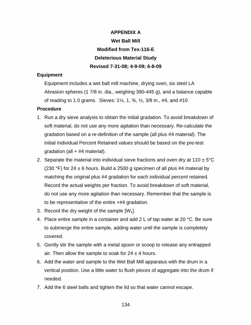
134

APPENDIX A

Wet Ball Mill

Modified from Tex-116-E

Deleterious Material Study

Revised 7-31-08; 4-9-09; 6-8-09

Equipment

Equipment includes a wet ball mill machine, drying oven, six steel LA

Abrasion spheres (1 7/8 in. dia., weighing 390-445 g), and a balance capable

of reading to 1.0 grams. Sieves: 1½, 1, ¾, ½, 3/8 in., #4, and #10

Procedure

1. Run a dry sieve analysis to obtain the initial gradation. To avoid breakdown of

soft material, do not use any more agitation than necessary. Re-calculate the

gradation based on a re-definition of the sample (all plus #4 material). The

initial Individual Percent Retained values should be based on the pre-test

gradation (all + #4 material).

2. Separate the material into individual sieve fractions and oven dry at 110 ± 5°C

(230 °F) for 24 ± 6 hours. Build a 2500 g specimen of all plus #4 material by

matching the original plus #4 gradation for each individual percent retained.

Record the actual weights per fraction. To avoid breakdown of soft material,

do not use any more agitation than necessary. Remember that the sample is

to be representative of the entire +#4 gradation.

3. Record the dry weight of the sample [W1].

4. Place entire sample in a container and add 2 L of tap water at 20 °C. Be sure

to submerge the entire sample, adding water until the sample is completely

covered.

5. Gently stir the sample with a metal spoon or scoop to release any entrapped

air. Then allow the sample to soak for 24 ± 4 hours.

6. Add the water and sample to the Wet Ball Mill apparatus with the drum in a

vertical position. Use a little water to flush pieces of aggregate into the drum if

needed.

7. Add the 6 steel balls and tighten the lid so that water cannot escape.

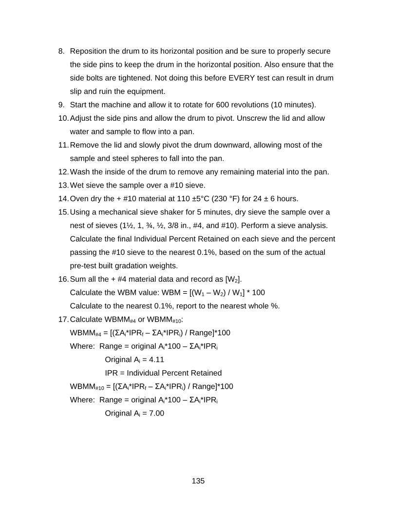
135

8. Reposition the drum to its horizontal position and be sure to properly secure

the side pins to keep the drum in the horizontal position. Also ensure that the

side bolts are tightened. Not doing this before EVERY test can result in drum

slip and ruin the equipment.

9. Start the machine and allow it to rotate for 600 revolutions (10 minutes).

10. Adjust the side pins and allow the drum to pivot. Unscrew the lid and allow

water and sample to flow into a pan.

11. Remove the lid and slowly pivot the drum downward, allowing most of the

sample and steel spheres to fall into the pan.

12. Wash the inside of the drum to remove any remaining material into the pan.

13. Wet sieve the sample over a #10 sieve.

14. Oven dry the + #10 material at 110 ±5°C (230 °F) for 24 ± 6 hours.

15. Using a mechanical sieve shaker for 5 minutes, dry sieve the sample over a

nest of sieves (1½, 1, ¾, ½, 3/8 in., #4, and #10). Perform a sieve analysis.

Calculate the final Individual Percent Retained on each sieve and the percent

passing the #10 sieve to the nearest 0.1%, based on the sum of the actual

pre-test built gradation weights.

16. Sum all the + #4 material data and record as [W2].

Calculate the WBM value: WBM = [(W1 – W2) / W1] * 100

Calculate to the nearest 0.1%, report to the nearest whole %.

17. Calculate WBMM#4 or WBMM#10:

WBMM#4 = [(ΣAi*IPRf – ΣAi*IPRi) / Range]*100

Where: Range = original Ai*100 – ΣAi*IPRi

Original Ai = 4.11

IPR = Individual Percent Retained

WBMM#10 = [(ΣAi*IPRf – ΣAi*IPRi) / Range]*100

Where: Range = original Ai*100 – ΣAi*IPRi

Original Ai = 7.00

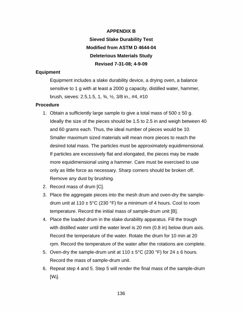
136

APPENDIX B

Sieved Slake Durability Test

Modified from ASTM D 4644-04

Deleterious Materials Study

Revised 7-31-08; 4-9-09

Equipment

Equipment includes a slake durability device, a drying oven, a balance

sensitive to 1 g with at least a 2000 g capacity, distilled water, hammer,

brush, sieves: 2.5,1.5, 1, ¾, ½, 3/8 in., #4, #10

Procedure

1. Obtain a sufficiently large sample to give a total mass of 500 ± 50 g.

Ideally the size of the pieces should be 1.5 to 2.5 in and weigh between 40

and 60 grams each. Thus, the ideal number of pieces would be 10.

Smaller maximum sized materials will mean more pieces to reach the

desired total mass. The particles must be approximately equidimensional.

If particles are excessively flat and elongated, the pieces may be made

more equidimensional using a hammer. Care must be exercised to use

only as little force as necessary. Sharp corners should be broken off.

Remove any dust by brushing.

2. Record mass of drum [C].

3. Place the aggregate pieces into the mesh drum and oven-dry the sample-

drum unit at 110 ± 5°C (230 °F) for a minimum of 4 hours. Cool to room

temperature. Record the initial mass of sample-drum unit [B].

4. Place the loaded drum in the slake durability apparatus. Fill the trough

with distilled water until the water level is 20 mm (0.8 in) below drum axis.

Record the temperature of the water. Rotate the drum for 10 min at 20

rpm. Record the temperature of the water after the rotations are complete.

5. Oven-dry the sample-drum unit at 110 ± 5°C (230 °F) for 24 ± 6 hours.

Record the mass of sample-drum unit.

6. Repeat step 4 and 5. Step 5 will render the final mass of the sample-drum

[Wf].

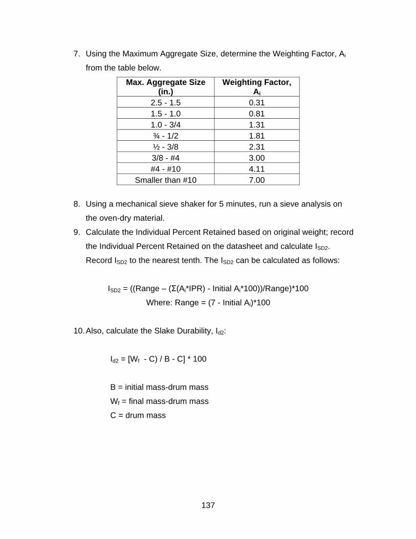
137

7. Using the Maximum Aggregate Size, determine the Weighting Factor, Ai

from the table below.

Max. Aggregate Size (in.)

Weighting Factor, Ai

2.5 - 1.5 0.31 1.5 - 1.0 0.81 1.0 - 3/4 1.31 ¾ - 1/2 1.81 ½ - 3/8 2.31 3/8 - #4 3.00 #4 - #10 4.11

Smaller than #10 7.00

8. Using a mechanical sieve shaker for 5 minutes, run a sieve analysis on

the oven-dry material.

9. Calculate the Individual Percent Retained based on original weight; record

the Individual Percent Retained on the datasheet and calculate ISD2.

Record ISD2 to the nearest tenth. The ISD2 can be calculated as follows:

ISD2 = ((Range – (Σ(Ai*IPR) - Initial Ai*100))/Range)*100

Where: Range = (7 - Initial Ai)*100

10. Also, calculate the Slake Durability, Id2:

Id2 = [Wf - C) / B - C] * 100

B = initial mass-drum mass

Wf = final mass-drum mass

C = drum mass

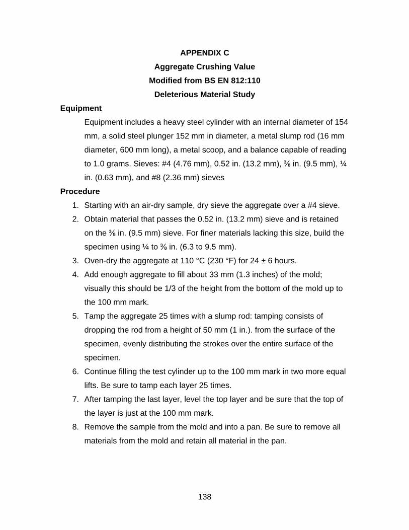
138

APPENDIX C


Modified from BS EN 812:110

Deleterious Material Study

Equipment

Equipment includes a heavy steel cylinder with an internal diameter of 154

mm, a solid steel plunger 152 mm in diameter, a metal slump rod (16 mm

diameter, 600 mm long), a metal scoop, and a balance capable of reading

to 1.0 grams. Sieves: #4 (4.76 mm), 0.52 in. (13.2 mm), ⅜ in. (9.5 mm), ¼

in. (0.63 mm), and #8 (2.36 mm) sieves

Procedure

1. Starting with an air-dry sample, dry sieve the aggregate over a #4 sieve.

2. Obtain material that passes the 0.52 in. (13.2 mm) sieve and is retained

on the ⅜ in. (9.5 mm) sieve. For finer materials lacking this size, build the

specimen using ¼ to ⅜ in. (6.3 to 9.5 mm).

3. Oven-dry the aggregate at 110 °C (230 °F) for 24 ± 6 hours.

4. Add enough aggregate to fill about 33 mm (1.3 inches) of the mold;

visually this should be 1/3 of the height from the bottom of the mold up to

the 100 mm mark.

5. Tamp the aggregate 25 times with a slump rod: tamping consists of

dropping the rod from a height of 50 mm (1 in.). from the surface of the

specimen, evenly distributing the strokes over the entire surface of the

specimen.

6. Continue filling the test cylinder up to the 100 mm mark in two more equal

lifts. Be sure to tamp each layer 25 times.

7. After tamping the last layer, level the top layer and be sure that the top of

the layer is just at the 100 mm mark.

8. Remove the sample from the mold and into a pan. Be sure to remove all

materials from the mold and retain all material in the pan.

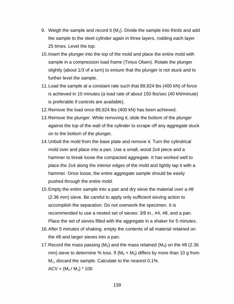
139

9. Weigh the sample and record it (M1). Divide the sample into thirds and add

the sample to the steel cylinder again in three layers, rodding each layer

25 times. Level the top.

10. Insert the plunger into the top of the mold and place the entire mold with

sample in a compression load frame (Tinius Olsen). Rotate the plunger

slightly (about 1/3 of a turn) to ensure that the plunger is not stuck and to

further level the sample.

11. Load the sample at a constant rate such that 89,924 lbs (400 kN) of force

is achieved in 10 minutes (a load rate of about 150 lbs/sec (40 kN/minute)

is preferable if controls are available).

12. Remove the load once 89,924 lbs (400 kN) has been achieved.

13. Remove the plunger. While removing it, slide the bottom of the plunger

against the top of the wall of the cylinder to scrape off any aggregate stuck

on to the bottom of the plunger.

14. Unbolt the mold from the base plate and remove it. Turn the cylindrical

mold over and place into a pan. Use a small, wood 2x4 piece and a

hammer to break loose the compacted aggregate. It has worked well to

place the 2x4 along the interior edges of the mold and lightly tap it with a

hammer. Once loose, the entire aggregate sample should be easily

pushed through the entire mold.

15. Empty the entire sample into a pan and dry sieve the material over a #8

(2.36 mm) sieve. Be careful to apply only sufficient sieving action to

accomplish the separation. Do not overwork the specimen. It is

recommended to use a nested set of sieves: 3/8 in., #4, #8, and a pan.

Place the set of sieves filled with the aggregate in a shaker for 5 minutes.

16. After 5 minutes of shaking, empty the contents of all material retained on

the #8 and larger sieves into a pan.

17. Record the mass passing (M2) and the mass retained (M3) on the #8 (2.36

mm) sieve to determine % loss. If (M2 + M3) differs by more than 10 g from

M1, discard the sample. Calculate to the nearest 0.1%.

ACV = (M2 / M1) * 100

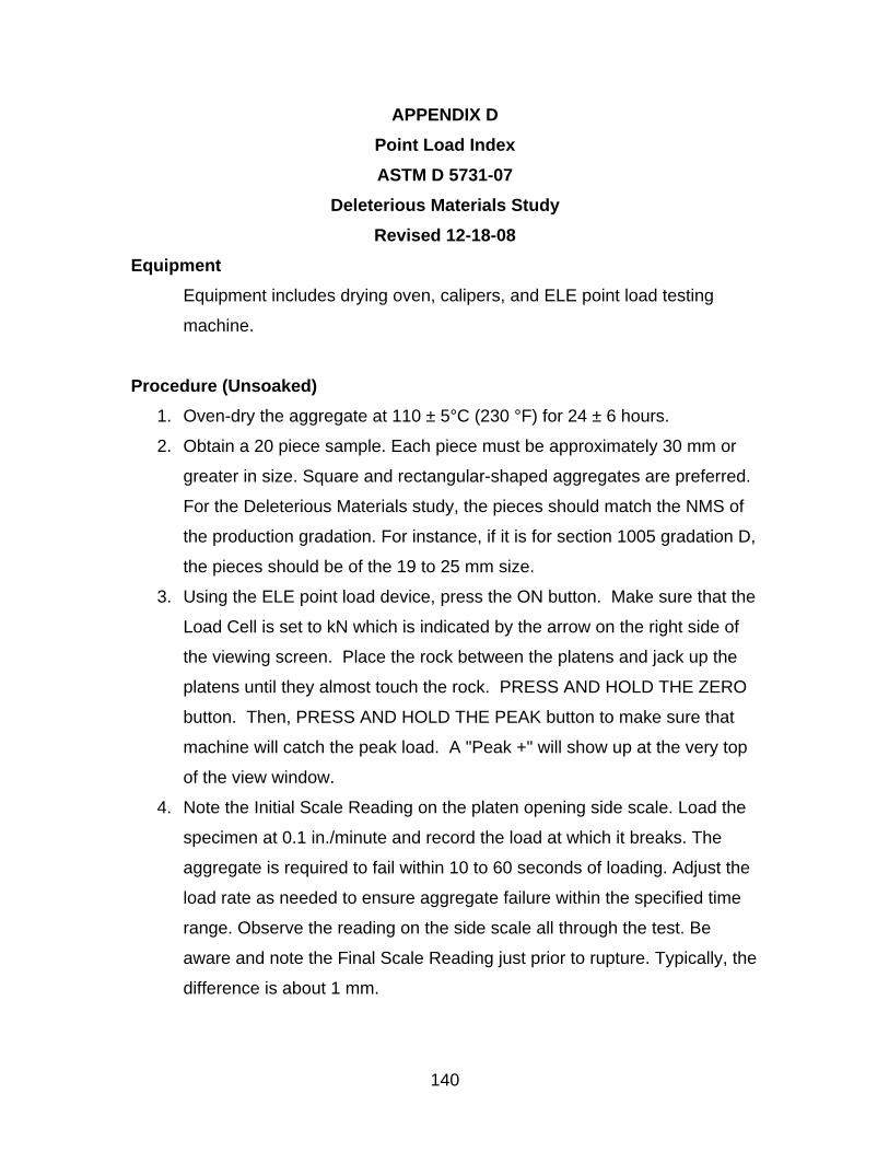
140

APPENDIX D

Point Load Index

ASTM D 5731-07


Revised 12-18-08

Equipment

Equipment includes drying oven, calipers, and ELE point load testing

machine.

Procedure (Unsoaked)

1. Oven-dry the aggregate at 110 ± 5°C (230 °F) for 24 ± 6 hours.

2. Obtain a 20 piece sample. Each piece must be approximately 30 mm or

greater in size. Square and rectangular-shaped aggregates are preferred.

For the Deleterious Materials study, the pieces should match the NMS of

the production gradation. For instance, if it is for section 1005 gradation D,

the pieces should be of the 19 to 25 mm size.

3. Using the ELE point load device, press the ON button. Make sure that the

Load Cell is set to kN which is indicated by the arrow on the right side of

the viewing screen. Place the rock between the platens and jack up the

platens until they almost touch the rock. PRESS AND HOLD THE ZERO

button. Then, PRESS AND HOLD THE PEAK button to make sure that

machine will catch the peak load. A "Peak +" will show up at the very top

of the view window.

4. Note the Initial Scale Reading on the platen opening side scale. Load the

specimen at 0.1 in./minute and record the load at which it breaks. The

aggregate is required to fail within 10 to 60 seconds of loading. Adjust the

load rate as needed to ensure aggregate failure within the specified time

range. Observe the reading on the side scale all through the test. Be

aware and note the Final Scale Reading just prior to rupture. Typically, the

difference is about 1 mm.

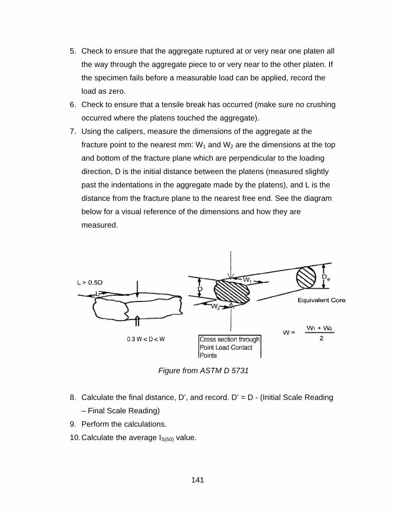
141

5. Check to ensure that the aggregate ruptured at or very near one platen all

the way through the aggregate piece to or very near to the other platen. If

the specimen fails before a measurable load can be applied, record the

load as zero.

6. Check to ensure that a tensile break has occurred (make sure no crushing

occurred where the platens touched the aggregate).

7. Using the calipers, measure the dimensions of the aggregate at the

fracture point to the nearest mm: W1 and W2 are the dimensions at the top

and bottom of the fracture plane which are perpendicular to the loading

direction, D is the initial distance between the platens (measured slightly

past the indentations in the aggregate made by the platens), and L is the

distance from the fracture plane to the nearest free end. See the diagram

below for a visual reference of the dimensions and how they are

measured.

Figure from ASTM D 5731

8. Calculate the final distance, D’, and record. D’ = D - (Initial Scale Reading

– Final Scale Reading)

9. Perform the calculations.

10. Calculate the average IS(50) value.

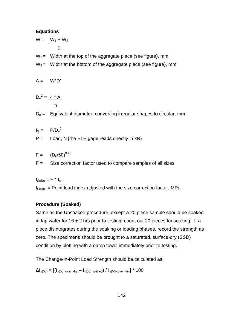
142

Equations

W = W1 + W2

2

W1 = Width at the top of the aggregate piece (see figure), mm

W2 = Width at the bottom of the aggregate piece (see figure), mm

A = W*D’

De2 = 4 * A

π

De = Equivalent diameter, converting irregular shapes to circular, mm

IS = P/De2

P = Load, N [the ELE gage reads directly in kN)

F = (De/50)0.45

F = Size correction factor used to compare samples of all sizes

IS(50) = F * Is

IS(50) = Point load index adjusted with the size correction factor, MPa

Procedure (Soaked)

Same as the Unsoaked procedure, except a 20 piece sample should be soaked

in tap water for 16 ± 2 hrs prior to testing: count out 20 pieces for soaking. If a

piece disintegrates during the soaking or loading phases, record the strength as

zero. The specimens should be brought to a saturated, surface-dry (SSD)

condition by blotting with a damp towel immediately prior to testing.

The Change-in-Point Load Strength should be calculated as: ΔIs(50) = [(Is(50),oven dry – Is(50),soaked) / Is(50),oven dry] * 100

143

APPENDIX E

Methylene Blue AASHTO T 330-07

Deleterious Materials Study Revised 7-31-08

Revised 12-18-08 Revised 6-12-09

Equipment

Equipment includes a 500 ml Griffin beaker, one magnetic mixing plate

with stir bar, one amber-colored burette of at least 50 ml capacity with 0.1

ml graduations, one glass rod, one glass funnel, and Whatman No. 2 filter

paper. A 200 ml capacity volumetric flask and a balance capable of

reading to 1.00 grams.

Methylene Blue reagent should be stored for no more than 4 months in a

brown bottle wrapped in foil inside of a dark cabinet at lab temperature.

Sieves: #200

Solution Mixing Procedures

1. Place 1 gram of methylene blue dye into a 500 ml Griffin beaker.

2. Add about 150 ml of distilled water at lab temperature to the beaker

3. Mix thoroughly using the magnetic stirrer.

4. Using the funnel, pour the solution into the 200 ml volumetric flask. Rinse

all of the remaining solution into the flask.

5. Add distilled water to bring the solution level to the 200 ml mark of the

volumetric flask and shake.

6. Add the solution to the burette as necessary.

METHOD A

Procedure

1. Using some material processed for the PI tests (minus #40), dry sieve

over a #200 sieve.

2. Oven-dry the minus #200 material at 60 ± 5°C (140°F) for 24 ± 6 hours.

3. Weigh a 10.00 ± 0.05 gram sample of minus #200 material [W].

4. Flush the burette with methylene blue solution by filling it with 25 ml of

solution, then opening the valve and allowing the entire 25 ml of solution

144

to drain into a beaker. This is done to ensure that water in the burette is

not left to dilute the solution. Flushing removes water. Discard the solution

once drained.

5. Fill the burette with the methylene blue solution.

6. Place the sample in the Griffin beaker and add 30 ml of distilled water.

7. Place the Griffin beaker on a magnetic mixing plate and insert the magnet

into the beaker.

8. Mix the sample and water to create a slurry. Do not mix at an excessive

rate, as this may cause foaming, which may inhibit the moisture escape

during the drop test.

9. With the slurry mixing, add 0.5 ml of the solution. Allow to mix for 1

minute.

10. If a sample has been previously tested: it is permissible to add more than

0.5 ml, up to 2.0 ml less than what has been required for previous

samples to reach titration. (Example: if a previous sample has taken 16 ml

to reach titration, it is permissible to immediately add 14 ml on the first

dose of a subsequent specimen. If the light blue halo appears on this first

round, then the sample must be discarded and the first dose must be

lessened by at least 2.0 ml). This step is allowed to reduce the amount of

time required to run replicate tests.

11. Using the glass rod, place a single drop of the slurry on a filter paper to

check for a light blue halo surrounding the dark blue dyed solids

(signifying a fulfilled cation exchange capacity). Ignore the moisture halo.

12. Continue to add 0.5 ml increments, mix, and check until the light blue halo

appears. Larger increments can be used, especially at the beginning of

the test, if it is known that the sample’s adsorption of the dye is high.

13. Once the light blue halo is achieved, mix the solution for an additional 5

minutes and place another drop on filter paper to ensure that the

exchange capacity is met (e.g. if the light blue halo does not appear, the

end point has not been achieved. Continue titration as before).

145

14. Record volume of solution required for titration [V] and calculate the

Methylene Blue Value [MBV].

15. Rinse the burette with distilled water; allow to drain by leaving the petcock

open.

Calculate MBV to the nearest 0.1 mg/g

Formula: [MBV] = CV/W

Where : C = concentration of methylene blue dye in the

solution (mg/ml). “C” is equal to 5 if the solution is

made as directed in the instructions.

V = Amount of solution required for titration (ml)

W = Original oven-dry sample weight

METHOD B

Method B is performed the same as Method A with the exception of the origin of the material:

1. Save all material passing the #12 sieve from the LA Abrasion test and

further sieve over a #200 sieve. Proceed with Method A, step 2.

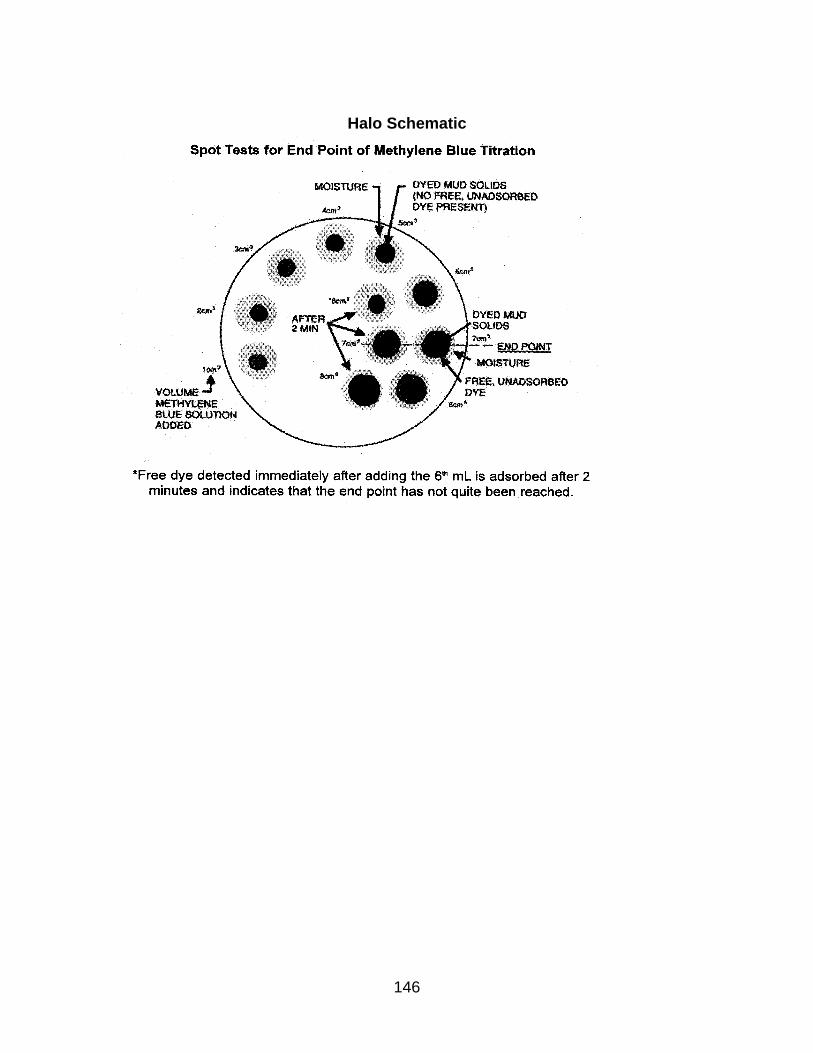
146

Halo Schematic

147

APPENDIX F Vacuum Saturated Specific Gravity and Absorption

Modified from AASHTO T 85


Revised 7-31-08; 6-8-09

Equipment

Equipment includes a 4500 ml pycnometer modified to introduce water, a

non-modified pycnometer, a vacuum pump capable of sustaining a vacuum

pressure of at least 25 mm of mercury (absolute pressure) with mercury

manometer with appropriate ancillary equipment such as a vacuum

regulator, and a towel. A weigh-in-water station should be available that

includes a water bath suitable for immersion of the suspended container with

its saturated specimen, an overflow outlet for maintaining a default water

level, a method for controlling or monitoring water temperature, a balance

with a weigh-below capability (nearest 0.1 g readability), and some type of

suspended platform on which the pycnometer can be supported while

submerged in the water bath. The platform and rod/wires that connect the

platform to the balance should displace a minimum amount of water.

Procedure

1. Obtain a sample size appropriate for the gradation. MoDOT 1005 Gradation F

requires a 2000 gram sample. MoDOT 1005 Gradation D and 1007 Type 5

require a 3000 gram sample, and MoDOT Gradation B requires a 4000 gram

sample.

2. Split the material over a #4 sieve. Work with the plus #4 material.

3. Do not wash the material.

4. Oven-dry the aggregate at 110 ± 5 °C (230 ± 9 °F) for 24 ± 6 hours. Cool to

room temperature (25 ± 5 °C).

5. Bring the test water to 25 ± 5 °C.

6. Place the specimen in the modified pycnometer and attach the pycnometer to

a vacuum apparatus. Close the vent valve on the mercury manometer. Turn

on the vacuum pump by setting the timer to an arbitrary value such as 45

148

minutes then switching on the timer (the pump is connected to the timer).

Gradually increase the vacuum to 27.5 ± 2.5 mm of mercury absolute

pressure as measured by the mercury manometer. As soon as this level is

reached, reset the timer to 30 minutes. Allow the aggregate to sit under

vacuum for 5.0 minutes ± 15 sec from the time the timer was set to 30

minutes.

7. After the 5.0 minute period, while the vacuum pump is still running, turn the

valve that is connected to the water slowly to the open position. Allow the

pycnometer to fill with water until at least one inch of water is over the top of

the aggregate. Then shut off the valve to the water. Start the mechanical

agitator and turn the setting to 8.

8. When the timer goes off, the vacuum pump will automatically stop (30

minutes at 27.5 ± 2.5 mm of mercury absolute pressure will have been

achieved). Stop the mechanical agitation.

9. Using the vent valve on the mercury manometer, slowly release the vacuum

at a rate not to exceed 2.36 inches mercury gage per second as displayed on

the vacuum gage on the lid of the pycnometer.

10. Remove the lid from the pycnometer.

11. Place an empty pan in a water bath. Without exposing the aggregate to the

air, carefully submerge the pycnometer in the water and, while underwater,

empty the contents of the pycnometer into the pan. Be sure that the

pycnometer and aggregate are completely submerged when transferring the

aggregate. Avoid loss of material.

12. Remove the pycnometer from the bath.

13. Carefully remove the pan filled with aggregate from the water bath. Decant

some of the water, but leave about 2 inches of water above the surface of the

aggregate and allow the specimen to sit for 24 ± 2 hours.

14. After 24 ± 2 hours, drain water from aggregate over a #8 screen (taking care

not to let the aggregate lose its saturated surface–wet condition) and roll

aggregate in a pre-dampened towel to obtain SSD state. The SSD state is

reached when the sheen on the aggregate just barely disappears.

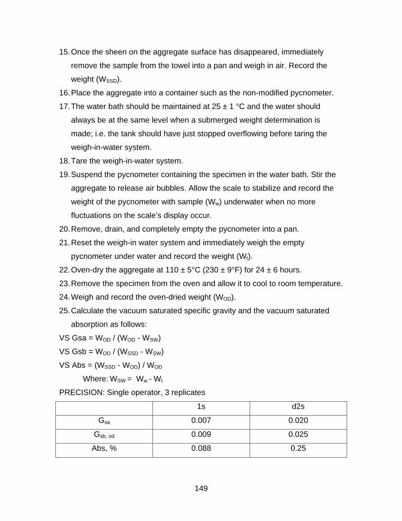
149

15. Once the sheen on the aggregate surface has disappeared, immediately

remove the sample from the towel into a pan and weigh in air. Record the

weight (WSSD).

16. Place the aggregate into a container such as the non-modified pycnometer.

17. The water bath should be maintained at 25 ± 1 °C and the water should

always be at the same level when a submerged weight determination is

made; i.e. the tank should have just stopped overflowing before taring the

weigh-in-water system.

18. Tare the weigh-in-water system.

19. Suspend the pycnometer containing the specimen in the water bath. Stir the

aggregate to release air bubbles. Allow the scale to stabilize and record the

weight of the pycnometer with sample (Ww) underwater when no more

fluctuations on the scale’s display occur.

20. Remove, drain, and completely empty the pycnometer into a pan.

21. Reset the weigh-in water system and immediately weigh the empty

pycnometer under water and record the weight (Wt).

22. Oven-dry the aggregate at 110 ± 5°C (230 ± 9°F) for 24 ± 6 hours.

23. Remove the specimen from the oven and allow it to cool to room temperature.

24. Weigh and record the oven-dried weight (WOD).

25. Calculate the vacuum saturated specific gravity and the vacuum saturated

absorption as follows:

VS Gsa = WOD / (WOD - WSW)

VS Gsb = WOD / (WSSD - WSW)

VS Abs = (WSSD - WOD) / WOD

Where: WSW = Ww - Wt

PRECISION: Single operator, 3 replicates

1s d2s

Gsa 0.007 0.020

Gsb, od 0.009 0.025

Abs, % 0.088 0.25

150

APPENDIX G

CORRELATION MATRIX

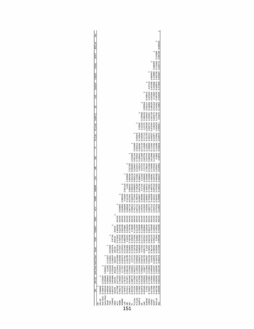
151

DR

DR

+S

CS

oft

Chert

Hard

Ch

ert

Shale

TD

MT

DM

HC

NM

SA

CV

WB

MW

BM

MLA

AM

BM

DP

IP

LS

,dry

PLS

,wet

DeltP

LS

SE

Isd2

So

dS

ulf

VS

BS

GV

SA

bs

WA

FT

BS

G,o

dA

bs

DR

1 DR+

SC

0.9

99994

1S

oft

Chert

-0.2

36678

-0.2

3338

41

Hard

Chert

-0.0

55234

-0.0

5508

60.0

5533

11

Sha

le0.6

99165

0.6

9885

4-0

.253

50.1

138

17

1T

DM

0.9

84537

0.9

8446

5-0

.25194

9-0

.0168

41

0.8

13

584

1T

DM

HC

0.9

53707

0.9

5366

8-0

.23528

30.1

965

25

0.8

22

079

0.9

7705

1N

MS

#D

IV/0

!#D

IV/0

!#D

IV/0

!#

DIV

/0!

#D

IV/0

!#D

IV/0

!#D

IV/0

!1

AC

V0.6

77096

0.6

7722

5-0

.12194

3-0

.3219

08

0.0

91

319

0.5

72

942

0.4

93269

#D

IV/0

!1

WB

M0.7

89174

0.7

8929

3-0

.15141

8-0

.3344

59

0.2

73

337

0.7

08

724

0.6

23749

#D

IV/0

!0.9

3989

41

WB

MM

0.8

12191

0.8

1225

4-0

.1725

7-0

.3416

79

0.3

16

015

0.7

37

866

0.6

50788

#D

IV/0

!0.9

1894

60.9

9023

61

LA

A0.7

87672

0.7

8725

7-0

.30400

4-0

.2574

41

0.2

41

463

0.6

99

245

0.6

30861

#D

IV/0

!0.9

4830

90.9

344

50.9

311

18

1M

B0.5

76211

0.5

7497

1-0

.49115

50.1

657

89

0.6

22

906

0.6

2031

0.6

43619

#D

IV/0

!0.0

8694

80.1

5116

20.2

09

0.3

53

606

1M

D0.8

44814

0.8

4454

6-0

.27540

6-0

.2217

14

0.3

26

892

0.7

66

786

0.7

04706

#D

IV/0

!0.8

6772

40.8

7264

10.8

602

52

0.8

92

404

0.3

21

335

1P

I-0

.487254

-0.4

8677

90.2

5065

10.2

72

72

-0.1

62

608

-0.4

35

625

-0.3

6909

#D

IV/0

!-0

.59961

9-0

.56613

3-0

.5892

16

-0.6

43

128

-0.0

94

805

-0.5

19309

1P

LS

,dry

-0.3

72161

-0.3

7268

3-0

.06227

20.7

151

53

0.1

16

728

-0.2

74

305

-0.1

16638

#D

IV/0

!-0

.79117

2-0

.72754

4-0

.6996

03

-0.6

83

115

0.2

26

647

-0.6

5110

60.6

31969

1P

LS

,wet

-0.4

40868

-0.4

4072

10.1

4563

30.5

960

63

0.0

55

429

-0.3

44

662

-0.2

11003

#D

IV/0

!-0

.80712

1-0

.76827

9-0

.7282

94

-0.7

10

481

0.2

14

072

-0.7

63532

0.5

94314

0.9

3353

11

DeltP

LS

-0.3

71897

-0.3

7339

6-0

.34234

60.5

948

73

0.0

48

286

-0.2

91

685

-0.1

59306

#D

IV/0

!-0

.63924

7-0

.63805

7-0

.6417

66

-0.5

96

913

-0.0

0514

-0.4

0944

10.4

09281

0.7

3054

40.4

928

11

SE

-0.0

32978

-0.0

3116

80.5

2662

2-0

.0407

92

-0.3

7533

-0.1

17

472

-0.1

23888

#D

IV/0

!0.4

4970

20.3

5049

50.2

71

42

0.2

2342

-0.6

7524

0.2

11899

-0.2

71734

-0.5

4838

2-0

.5219

2-0

.3494

56

1Is

d2

-0.8

20185

-0.8

2055

50.0

867

70.0

547

25

-0.6

95

722

-0.8

37

823

-0.8

09942

#D

IV/0

!-0

.52355

3-0

.65050

5-0

.6585

61

-0.6

06

003

-0.5

7276

-0.6

29736

0.1

41698

0.2

1711

20.2

372

20.3

652

28

0.0

85

944

1S

od

Sulf

0.3

761

0.3

7680

80.1

1459

30.0

436

47

0.1

053

0.3

32

161

0.3

35028

#D

IV/0

!0.4

6509

30.3

9496

70.4

065

15

0.4

26

983

0.1

98

241

0.5

37476

0.1

26361

-0.2

3178

3-0

.25634

5-0

.2493

24

0.0

32

107

-0.3

48

015

1V

SB

SG

-0.7

44007

-0.7

4380

10.2

3385

4-0

.0512

59

-0.2

38

501

-0.6

63

192

-0.6

61272

#D

IV/0

!-0

.69077

3-0

.75699

3-0

.7366

81

-0.7

63

689

-0.3

14

484

-0.8

8055

80.2

98989

0.4

0221

10.5

6273

20.2

559

51

-0.1

65

882

0.5

23

453

-0.5

7119

1V

SA

bs

0.6

77066

0.6

7606

4-0

.44654

80.3

41

81

0.3

81

144

0.6

43

143

0.7

03509

#D

IV/0

!0.3

7721

30.4

5263

80.4

697

03

0.5

95

961

0.7

30

095

0.6

13998

-0.1

72364

0.0

5832

7-0

.07034

4-0

.0417

28

-0.2

99

194

-0.5

01

004

0.4

37936

-0.8

00043

1W

AF

T0.1

57083

0.1

5663

9-0

.16433

7-0

.1695

25

0.2

88

335

0.1

98

113

0.1

58162

#D

IV/0

!-0

.05971

6-0

.16215

1-0

.0875

19

0.0

29

737

0.5

15

242

0.1

10624

-0.1

701

82

-0.0

1397

70.0

843

40.0

020

73

-0.5

21

918

-0.1

3805

0.2

46588

0.1

09886

0.0

8505

51

BS

G,o

d-0

.681708

-0.6

8159

50.2

0593

5-0

.1054

79

-0.0

16

594

-0.6

943

-0.7

49912

#D

IV/0

!-0

.57533

5-0

.56025

1-0

.4763

09

-0.6

45

068

-0.2

02

627

-0.8

569

0.1

01488

0.3

7606

10.5

5402

90.1

179

34

-0.2

43

361

0.4

30

795

-0.6

28576

0.9

50756

-0.7

3184

90.1

2458

61

0.5

63098

0.5

6231

8-0

.30119

40.3

853

76

0.3

72

498

0.5

90

399

0.7

60499

#D

IV/0

!0.2

4465

40.2

5989

60.1

964

34

0.4

60

247

0.6

18

584

0.5

8976

0.0

49834

0.0

393

75

-0.0

9551

70.0

44

75

-0.1

39

801

-0.5

44

525

0.4

71859

-0.8

16087

0.9

2577

20.0

0078

9-0

.8481

83

1A

bs

Missouri Department of Transportation Organizational Results P. O. Box 270 Jefferson City, MO 65102

573.526.4335 1 888 ASK MODOT [email protected]

quick test for percent of deleterious material -...

Documents