quick summary of tutorial data set - astron · fourth lofar data processing school, september 2016,...

Fourth LOFAR data processing school, September 2016, Tutorial 1

Quick summary of tutorial data set

* Seven sub-array pointings, frequency range 120.1 – 125.8 MHz* Hexagonal pattern centred at RA 21:00:00.00, Dec. +52:54:00.0 (Galactic Plane field)* Same fields as from a LOFAR 'radio sky monitor' programme (Transients KSP) * Calibrator Cygnus A* Dutch stations only

Tutorial can be downloaded here:https://dl.dropboxusercontent.com/u/44848769/data_school_tutorial1_FINAL.pdf


Tutorial 1: flagging, averaging and demixing

Jess Broderick (ASTRON)

Goal: to inspect a LOFAR HBA measurement set of a particular target field, and carry out some initial basic processing in preparation for calibration (Tutorial 2).

Note: in this tutorial, '>' is used to indicate a new input line in the terminal. 1. Login sheet

2. Log in to CEP3

You should have already received one of these. Your username = lodsXX, your reservation = tutorials_287, and your node = lof00Z.

Log in to the LOFAR portal:> ssh [email protected]

Log in to the head node, lhd002:> ssh lhd002

1


Activate a dummy session using your reservation:> use Slurm> srun - A tutorials - ‐reservation=tutorials_287 -N5 -u bash -i

Now, open a new terminal (and keep the previous one open too), typing the following commands:> ssh -Y [email protected] > ssh -Y lhd002> ssh -Y lof00Z

Verify that graphics forwarding works:> geany

To start with, we are just going to do some light processing. So let's go back to the head node:> exit

2

3. Initial inspection of the data using msoverview

The data sets for this tutorial can be found in lhd002:/data/scratch/DATASCHOOL16/T1. Let's have a quick look at these data to get an idea about the sizes of the measurement sets, as well as the naming convention used.> cd /data/scratch/DATASCHOOL16/T1> du -sh *uv.MS


The naming convention for each measurement set (also referred to as a sub-band) is Laaaaaa_SAPbbb_SBccc_uv.MS, where Laaaaaa is the observation/pipeline ID, SAPbbb is the sub-array pointing (beam), and SBccc is the sub-band number.

● What is the data volume per sub-band? In fact, there are 210 sub-bands for this observation (although we won't look at all of them in this tutorial): what is the total data volume then, and how does this compare with data from other telescopes that you may have used?

The next step is to take a closer look at the data. To do this, we load a set of standard software packages:> use Lofar

Now we can, for example, obtain a summary of a measurement set using msoverview: > msoverview in=L456104_SAP000_SB001_uv.MS

● Which field was observed? What was the duration of the observation? What was the centre frequency of this particular sub-band? How many channels (frequencies) are in the data set? What array configuration was used and what does the configuration name imply?

More detailed information in msoverview can be displayed using the 'verbose' argument: > msoverview in=L456104_SAP000_SB001_uv.MS verbose=T

● What is the number of time slots? What is the integration time per time step? How many stations (core and remote), and how many baselines? What is the relation between number of stations and baselines (excluding autocorrelations)?

3


You may have noticed the message 'This is a raw LOFAR MS (stored with LofarStMan)' in msoverview. This means that the data cannot be handled with Casa. Let's fix the problem. First, go back to your assigned compute node, and make a directory to do your work in. > ssh -Y lof00Z> cd /data/scratch> mkdir lodsXX ; cd lodsXX> mkdir T1 ; cd T1> use Lofar(note: we have to load the LOFAR packages again on this node)

Copy over sub-band SB001 to this directory: > scp -r lhd002:/data/scratch/DATASCHOOL16/T1/L456104_SAP000_SB001_uv.MS .

A simple DPPP (Default PreProcessing Pipeline) parset is required to make the data readablein Casa:> geany DPPP- makecopy.parset # (or vim, emacs, nano, nedit etc.)

Put the following commands in the parset and save it:msin=L456104_SAP000_SB001_uv.MS msout=L456104_SAP000_SB001_uv_copy.MS msin.autoweight=Truenumthreads=4 # so that the nodes are not overloaded, usually can skip this linesteps = [ ]

4


Let's take a look at the measurement set incasaplotms:> use Casa # initialize CASA software > casaplotms &

Open the measurement set from the GUI. Plot the XX correlation only by using the 'corr' argument(to speed things up). Select only cross correlations by typing '*&*' in the 'antenna' field (note: * - any antenna; & - cross correlations).

There are many large spikes, likely caused by RFI. Click on the 'Axes' tab and adjust the y-axisrange to something more sensible to find the real astronomical signal (e.g. max. = 1e+08).

● Does the y-axis scale make sense to you? What other plotting options could be useful?

5

4. casaplotms

Run DPPP on this parset:> DPPP DPPP- makecopy.parset

The output measurement set can now be opened using the standard Casa tools. Moreover, proper weighting of the data has been implemented (see the LOFAR cookbook for more information).


We can also further visualize the impact ofRFI in the measurement set using rfigui.

> rfigui L456104_SAP000_SB001_uv_copy.MS &

In the smaller menu that pops up, just choose ‘Open’. Then, in the new window, select index 0 (default) for antenna 1, and index 1 for antenna 2, before pressing 'Load'. This will plot the short intra-station baseline CS001HBA0 - CS001HBA1.

There is some clear narrow-band RFI. Createa power spectrum (under 'Plot').

● What could be causing the RFI? Are the fainter broadband structures at later times also RFI?

rfigui can flag the data using AOFlagger:'Actions'; 'Execute Strategy'. Also, find other useful plots in the plot menu.

● Would the plot look different if we had chosen e.g. a baseline between a core and remote station? Check this ('Go'; 'Go to...').

6

5. rfigui

Before flaggingAfter flagging

Channel 0 always flagged - edge effects due to polyphase filter


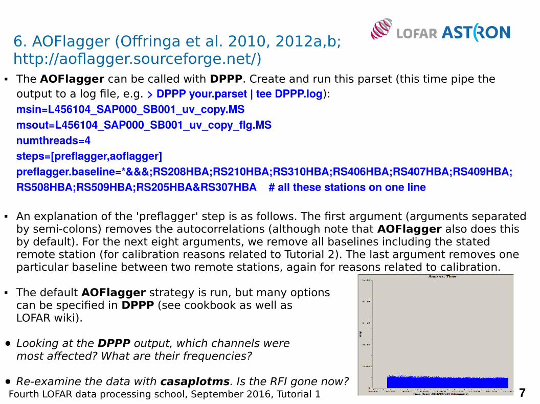
The AOFlagger can be called with DPPP. Create and run this parset (this time pipe the output to a log file, e.g. > DPPP your.parset | tee DPPP.log):msin=L456104_SAP000_SB001_uv_copy.MSmsout=L456104_SAP000_SB001_uv_copy_flg.MSnumthreads=4steps=[preflagger,aoflagger]preflagger.baseline=*&&&;RS208HBA;RS210HBA;RS310HBA;RS406HBA;RS407HBA;RS409HBA;RS508HBA;RS509HBA;RS205HBA&RS307HBA # all these stations on one line

An explanation of the 'preflagger' step is as follows. The first argument (arguments separated by semi-colons) removes the autocorrelations (although note that AOFlagger also does this by default). For the next eight arguments, we remove all baselines including the stated remote station (for calibration reasons related to Tutorial 2). The last argument removes one particular baseline between two remote stations, again for reasons related to calibration.

The default AOFlagger strategy is run, but many options can be specified in DPPP (see cookbook as well asLOFAR wiki).

● Looking at the DPPP output, which channels were most affected? What are their frequencies?

● Re-examine the data with casaplotms. Is the RFI gone now?

7

6. AOFlagger (Offringa et al. 2010, 2012a,b; http://aoflagger.sourceforge.net/)


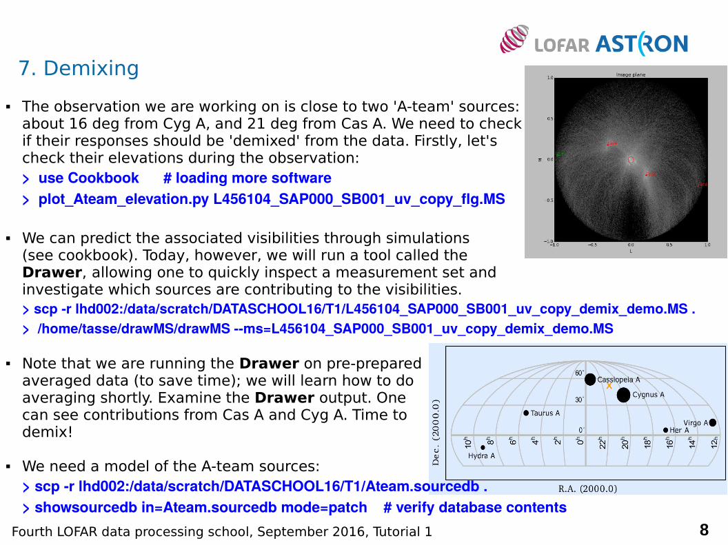
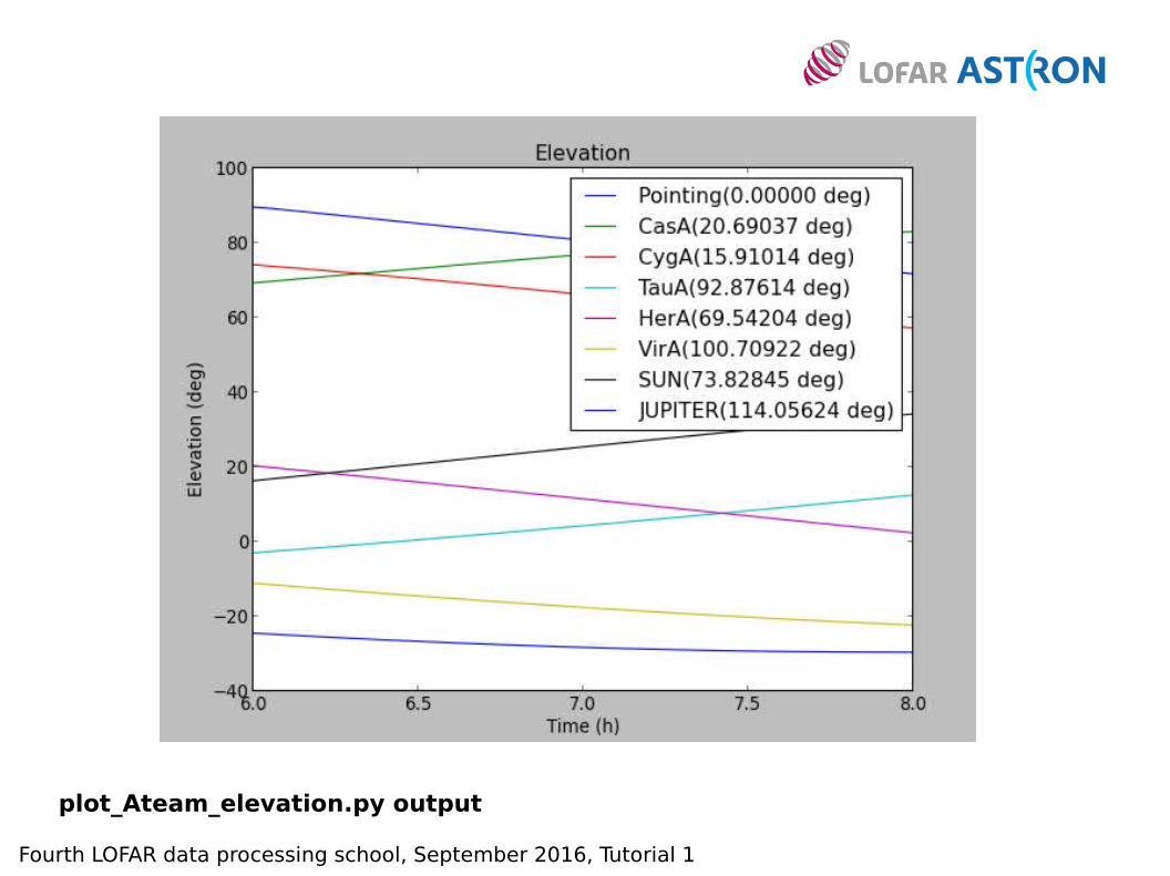
The observation we are working on is close to two 'A-team' sources:about 16 deg from Cyg A, and 21 deg from Cas A. We need to checkif their responses should be 'demixed' from the data. Firstly, let's check their elevations during the observation:> use Cookbook # loading more software > plot_Ateam_elevation.py L456104_SAP000_SB001_uv_copy_flg.MS

We can predict the associated visibilities through simulations (see cookbook). Today, however, we will run a tool called the Drawer, allowing one to quickly inspect a measurement set and investigate which sources are contributing to the visibilities.> scp -r lhd002:/data/scratch/DATASCHOOL16/T1/L456104_SAP000_SB001_uv_copy_demix_demo.MS .> /home/tasse/drawMS/drawMS --ms=L456104_SAP000_SB001_uv_copy_demix_demo.MS

Note that we are running the Drawer on pre-prepared averaged data (to save time); we will learn how to do averaging shortly. Examine the Drawer output. One can see contributions from Cas A and Cyg A. Time to demix!

We need a model of the A-team sources:> scp -r lhd002:/data/scratch/DATASCHOOL16/T1/Ateam.sourcedb .> showsourcedb in=Ateam.sourcedb mode=patch # verify database contents

8

7. Demixing

X


Use the following parset for DPPP:msin=L456104_SAP000_SB001_uv_copy_flg.MSmsout=L456104_SAP000_SB001_uv_copy_flg_demix_avg.MSnumthreads=4steps=[demix]demix.subtractsources=[CasA,CygA]demix.skymodel=Ateam.sourcedbdemix.timestep=10demix.freqstep=16demix.demixtimestep=60demix.demixfreqstep=64

The arguments 'timestep' and 'freqstep' compress the data in time and frequency, respectively, by the given factors.

Demixing two sources at once can be very time consuming. Thus, 'demixtimestep' and 'demixfreqstep' have been chosen to have rather coarse values (usually default to 'timestep' and 'freqstep' without needing to be specified).

● Run the Drawer again. Did we succeed in demixing Cyg A and Cas A from the data?> /home/tasse/drawMS/drawMS - -ms=L456104_SAP000_SB001_uv_copy_flg_demix_avg.MS

● What is the size of the compressed, demixed measurement set? Is this what you expect?

● Do you think that the time and frequency averaging settings are reasonable? How could they affect the calibration and imaging?

9


What if demixing is not needed? We can also just average in time and frequency. Here is a parset that could be run through DPPP:msin=L456104_SAP000_SB001_uv_copy_flg.MSmsout=L456104_SAP000_SB001_uv_copy_flg_avg.MSnumthreads=4steps=[averager]averager.timestep=10averager.freqstep=16

DPPP was designed to run pipelines containing multiple steps. Save the following parset as 'DPPP-all.parset', in preparation for the final part of the tutorial. This parset combines all the steps we have run in this tutorial, except that we skip demixing (too time consuming). msin=L456104_SAP000_SB001_uv.MSmsin.autoweight=true msout=L456104_SAP000_SB001_uv.MS.dpppnumthreads=4steps=[preflagger,aoflagger,averager]preflagger.baseline=*&&&;RS208HBA;RS210HBA;RS310HBA;RS406HBA;RS407HBA;RS409HBA;RS508HBA;RS509HBA;RS205HBA&RS307HBAaverager.timestep=10averager.freqstep=16

10

8. Averaging and combining tasks in DPPP


Clearly, it is impractical to do a manual reduction for a full observation of hundreds of sub-bands, although keep in mind that looking at your LOFAR data at least at some level is always highly recommended. Write a script (e.g. in Python or Bash) that will automate the process that we have just been through, applying it to the four sub-bands in the tutorial directory.

Firstly, note that you can download target sub-bands to your directory using a command like this:> scp -r lhd002:/data/scratch/DATASCHOOL16/T1/L456104_SAP000_SB000_uv.MS .

Secondly, you can override keys in your parset from the previous slide by specifying them on the command line, e.g.:> DPPP DPPP-all.parset msin=your.MS msout=your.MS.dppp

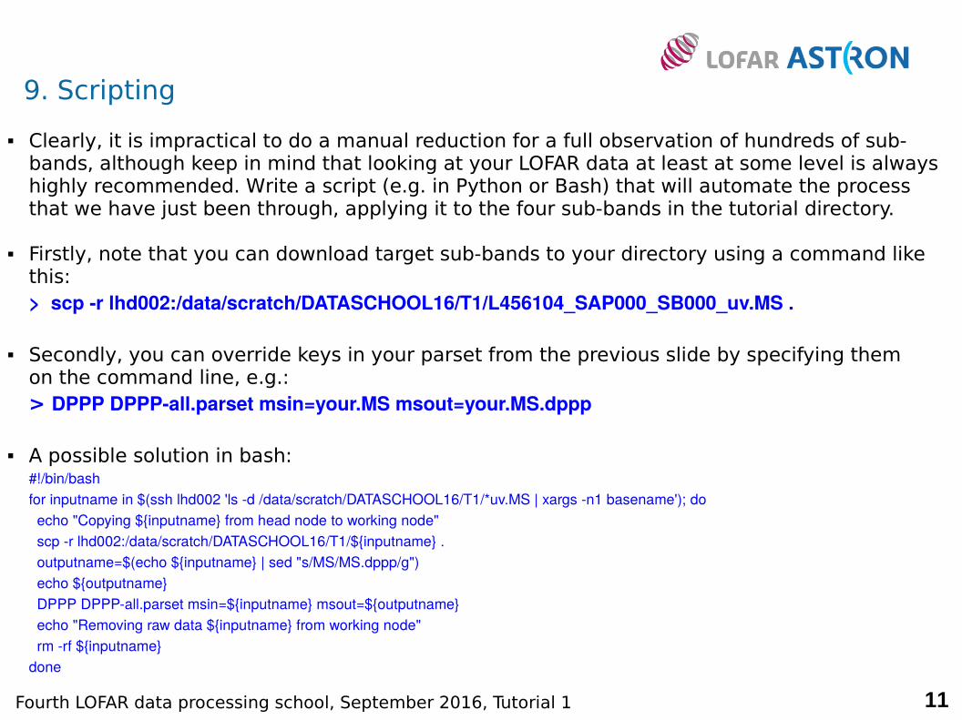
A possible solution in bash:#!/bin/bashfor inputname in $(ssh lhd002 'ls -d /data/scratch/DATASCHOOL16/T1/*uv.MS | xargs -n1 basename'); do echo "Copying ${inputname} from head node to working node" scp ‐r lhd002:/data/scratch/DATASCHOOL16/T1/${inputname} . outputname=$(echo ${inputname} | sed "s/MS/MS.dppp/g") echo ${outputname} DPPP DPPP-all.parset msin=${inputname} msout=${outputname} echo "Removing raw data ${inputname} from working node" rm -rf ${inputname}done

11

9. Scripting


This tutorial has given a brief overview of some of the initial processing steps for a LOFAR data set. It is highly recommended to also review chapters 2-4 in the cookbook, wheremore information can be found about the tools used in this tutorial, as well as other softwarethat is available.(http://www.astron.nl/radio-observatory/lofar/lofar-imaging-cookbook)

Time permitting, you could, for example, try the following:

(i) Simulating visibilities to predict A-team contributions: section 2.3.3 in the cookbook. Make sure to run any tests in a separate sub-directory on a dummy copy of the compressed data!

(ii) Experimenting with AOFlagger settings: section 3 in the cookbook.

Many/all of the steps in this tutorial can be carried out by the Radio Observatory as part of pre-processing. If in doubt about the best settings, always contact Science Support.

Always make sure to look at (at least some of) your data!!

12

10. Final remarks

After running your script, you should have four processed measurement sets (*.dppp). Use msoverview, casaplotms, etc. to verify that everything was processed successfully.


11. Extra slides / walkthrough

* Raw data volumes very large! * Total data rate can be ~few GB/s when using full 96 MHz bandwidth. * Data volume calculator athttp://lofar.astron.nl/service/pages/storageCalculator/calculate.jsp

Array config. - all core sub-stations and inner 24 tiles on remote stations. Same FoV per station. Often gives better quality images.

= cannot load in Casa(solution: tutorial slide 4)

Sub-array pointing


* Some of the verbose=T output from msoverview. * Note that the same sized diameter for core/remote stations (i.e. 'INNER' for the remote station tiles).

(62*61)/2 cross-correlation baselines = 1891 = 1953-62(note first station = no. 0in msoverview output)

CS – core stationRS – remote station

(note: no internationalstations in this data set)

HBA 0/1 – core station'ears'


N.B. only do this once at this stage!! Otherwise always = F (default)

This simple parset also automaticallyremoves clearly bad data if necessary (not here, though).


http://www.lofar.org/wiki/doku.php?id=public:user_software:ndppp


* Offringa et al. 2013, A&A, 549, A11NOTE: Significant RFI from DAB inter-modulation products above 150 MHz! See LOFAR technical webpages.

rfigui - also see http://www.astro.rug.nl/rfi-software/gui-tutorial.html

* Core-remote baseline – extended emission from target field resolved out (cf. tutorial slide 6). But RFI remains in this case...

Good practice to flag edge channels due to polyphase filter – e.g. chans 0,1,62,63 for a 64 chan MS. See DPPP info on wiki(preflag.chan)

* DPPP.log on Tutorial slide 7 – 98% flagged is the max. because chan 0 already flagged by default.General RFI occupancy quite low (~few per cent).


* The Drawer - http://www.lofar.org/wiki/lib/exe/fetch.php?media=commissioning:pres_drawer.pdf

* Demixing; usually default settings are fine. Look out for 'smart demixing' from LOFAR Cycle 8 onwards. Demixing paper: http://adsabs.harvard.edu/abs/2007ITSP...55.4497V (van der Tol et al. 2007)

* Worth putting in the time to make sure that you have some ideas of the possible effectsof the A-team on your data (and also in terms of the processing / observing time ratio). In the LBA you demix both Cyg A and Cas A by default, because the antenna elements can see the whole sky accessible from the LOFAR site. In the HBA, simulations can really help, but you are very likely to need demixing if an A-team source is less than about 20 deg from your target.

* Be a little bit careful with demix ignoretarget = F/T. F is generally best (and the default). If in doubt contact Science Support.

* Data averaging: what are your science goals? How much bandwidth/time smearing can you tolerate? How often should you be solving for the gain phases? Do you need to transfer large amounts of data to an external cluster first? Useful links:http://adsabs.harvard.edu/abs/1999ASPC..180..371B (Bridle & Schwab 1999)http://adsabs.harvard.edu/abs/2015A%26A...582A.123H (Heald et al. 2015; LOFAR MSSS)

One recommendation is to keep the time resolution to 10s maximum after averaging, and the minimum number of channels to 4 per sub-band (and quite possibly 8). Native time/frequency resolutions for the actual observations are typically 1 or 2s, and 64 chans/sub-band.

http://www.lofar.org/wiki/lib/exe/fetch.php?media=commissioning:pres_drawer.pdf

http://adsabs.harvard.edu/abs/2007ITSP...55.4497V

http://adsabs.harvard.edu/abs/1999ASPC..180..371B

http://adsabs.harvard.edu/abs/2015A%26A...582A.123H


plot_Ateam_elevation.py output


* Scripting – learning Python is a highly valuable skill!

* Important: <step>.type in DPPP - this defaults to the standard process name. But if you e.g. had custom step names like the following:

steps = [process1, process2, process3]

Then your parset needs extra lines such asprocess1.type=preflaggerprocess2.type=aoflaggerand so on.... See the LOFAR wiki for more information. And the example below.


https://casa.nrao.edu/docs/taskref/plotms-task.html

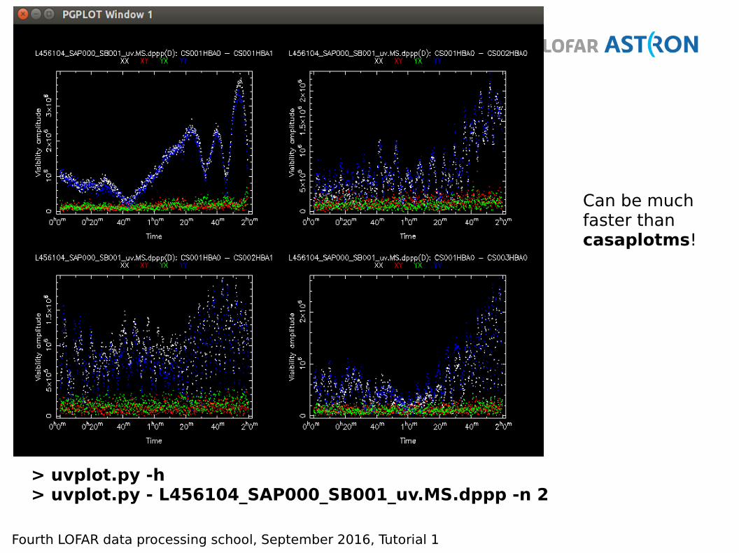
Not a surprise that amplitudes much higher on short baselines:Galactic Plane field, extended emission.Redo plot after calibration.


> uvplot.py -h> uvplot.py - L456104_SAP000_SB001_uv.MS.dppp -n 2

Can be muchfaster thancasaplotms!

quick summary of tutorial data set - astron · fourth lofar data processing school, september 2016,...

Documents