Quegel: A General-Purpose Query-Centric Framework forQuerying Big Graphs

Da Yan∗1, James Cheng∗2, M. Tamer Ozsu†3, Fan Yang∗4,Yi Lu∗5, John C. S. Lui∗6, Qizhen Zhang∗7, Wilfred Ng+8

∗Department of Computer Science and Engineering, The Chinese University of Hong Kong{1yanda, 2jcheng, 4fyang, 5ylu, 6cslui, 7qzzhang}@cse.cuhk.edu.hk

†David R. Cheriton School of Computer Science, University of Waterloo3tozsu@uwaterloo.ca

+Department of Computer Science and Engineering, The Hong Kong University of Science and Technology8wilfred@cse.ust.hk

ABSTRACTPioneered by Google’s Pregel, many distributed systems have beendeveloped for large-scale graph analytics. These systems exposethe user-friendly “think like a vertex” programming interface tousers, and exhibit good horizontal scalability. However, these sys-tems are designed for tasks where the majority of graph verticesparticipate in computation, but are not suitable for processing light-workload graph queries where only a small fraction of vertices needto be accessed. The programming paradigm adopted by these sys-tems can seriously under-utilize the resources in a cluster for graphquery processing. In this work, we develop a new open-source sys-tem, called Quegel, for querying big graphs, which treats queriesas first-class citizens in the design of its computing model. Usersonly need to specify the Pregel-like algorithm for a generic query,and Quegel processes light-workload graph queries on demand us-ing a novel superstep-sharing execution model to effectively utilizethe cluster resources. Quegel further provides a convenient inter-face for constructing graph indexes, which significantly improvequery performance but are not supported by existing graph-parallelsystems. Our experiments verified that Quegel is highly efficientin answering various types of graph queries and is up to orders ofmagnitude faster than existing systems.

1. INTRODUCTIONBig graphs are common in real-life applications today, for exam-

ple, online social networks and mobile communication networkshave billions of users, and web graphs and Semantic webs can beeven bigger. Processing such big graphs typically require a spe-cial infrastructure, and the most popular ones are Pregel [24] andPregel-like systems [1, 9, 10, 22, 29, 36]. In a Pregel-like system,a programmer thinks like a vertex and only needs to specify the be-havior of one vertex, and the system automatically schedules theexecution of the specified computing logic on all vertices. The sys-tem also handles fault tolerance and scales out without extra effort

from programmers.Existing Pregel-like systems, however, are designed for heavy-

weight graph computation (i.e., analytic workloads), where the ma-jority part of a graph or the entire graph is accessed. For example,Pregel’s PageRank algorithm [24] accesses the whole graph in eachiteration. However, many real-world applications involve varioustypes of graph querying, whose computation is light-weight in thesense that only a small portion of the input graph needs to be ac-cessed. For example, in our collaboration with researchers fromone of the world’s largest online shopping platforms, we have seenhuge demands for querying different aspects of big graphs for allsorts of analysis to boost sales and improve customer experience.In particular, they need to frequently examine the shortest-path dis-tance between some users in a large network extracted from theironline shopping data. While Pregel’s single-source shortest-path(SSSP) algorithm [24] can be applied here, much of the computa-tion will be wasted because only those paths between the queriedusers are of interest. Instead, it is much more efficient to applypoint-to-point shortest-path (PPSP) queries, which only traverse asmall part of the input graph. We also worked with a large tele-com operator, and our experience is that graph queries (with light-weight workloads) are integral parts of analyzing massive mobilephone and SMS networks.

The importance of querying big graphs has also been recognizedin some recent work [18], where two kinds of systems are iden-tified: (1) systems for offline graph analytics (such as Pregel andGraphLab) and (2) systems for online graph querying, includingHorton [30], G-SPARQL [28] and Trinity [32]. However, Hortonand G-SPARQL are tailor-made only for specific types of queries.Trinity supports graph query processing, but compared with Pregel,its main advantage is that it keeps the input graph in main memoriesso that the graph does not have to be re-loaded for each query. TheTrinity paper [32] also argues that indexing is too expensive for biggraphs and thus Trinity does not support indexing. In the VLDB2015 conference, there is also a workshop “Big-O(Q): Big GraphsOnline Querying”, but the works presented there only study algo-rithms for specific types of queries. So far, there lacks a general-purpose framework that allows users to easily design distributedalgorithms for answering various types of queries on big graphs.

One may, of course, use existing vertex-centric systems to pro-cess queries on big graphs, but these systems are not suitable forprocessing light-weight graph queries. To illustrate, consider pro-cessing PPSP queries on a 1.96-billion-edge Twitter graph usedin our experiments. To answer one query (s, t) by bidirectionalbreadth-first search (BiBFS) in our cluster, Giraph takes over 100

1

arX

iv:1

601.

0649

7v1

[cs

.DC

] 2

5 Ja

n 20

16

seconds, which is intolerable for a data analyst who wants to ex-amine the distance between users in an online social network withshort response time. To process queries on demand using an ex-isting vertex-centric system, a user has the following two options:(1) to process queries one after another, which leads to a low through-put since the communication workload of each query is usually toolight to fully utilize the network bandwidth and many synchroniza-tion barriers are incurred; or (2) to write a program to explicitlyprocess a batch of queries in parallel, which is not easy for usersand may not fully utilize the network bandwidth towards the end ofthe processing, since most queries may have finished their process-ing and only a small number of queries are still being processed. Itis also not clear how to use graph indexing for query processing inexisting vertex-centric systems.

To address the limitations of existing systems in querying biggraphs, we developed a distributed system, called Quegel, for large-scale graph querying. We implemented the Hub2-Labeling ap-proach [15] in Quegel, and it can achieve interactive speeds forPPSP querying on the same Twitter graph mentioned above. Quegeltreats queries as first-class citizens: users only need to write aPregel-like algorithm for processing a generic query, and the sys-tem automatically schedules the processing of multiple incomingqueries on demand. As a result, Quegel has a wide applicationscope, since any query that can be processed by a Pregel-stylevertex-centric algorithm can be answered by Quegel, and muchmore efficiently. Under this query-centric design, Quegel adoptsa novel superstep-sharing execution model to effectively utilize thecluster resources, and an efficient mechanism for managing ver-tex states that significantly reduces memory consumption. Quegelfurther provides a convenient interface for constructing indexes toimprove query performance. To our knowledge, Quegel is the firstgeneral-purpose programming framework for querying big graphsat interactive speeds on a distributed cluster. We have successfullyapplied Quegel to process five important types of graph queries (tobe presented in Section 5), and Quegel achieves performance up toorders of magnitude faster than existing systems.

The rest of this paper is organized as follows. We review relatedwork in Section 2. In Section 3, we highlight important concepts inthe design of Quegel, and key implementation issues. We introducethe programming model of Quegel in Section 4, and describe somegraph querying problems as well as their Quegel algorithms in Sec-tion 5. Finally, we evaluate the performance of Quegel in Section 6and conclude the paper in Section 7.

2. RELATED WORKWe first review existing vertex-centric graph-parallel systems.

We consider an input graph G=(V,E) stored on Hadoop distributedfile system (HDFS), where each vertex v ∈ V is associated with itsadjacency list (i.e., v’s neighbors). If G is undirected, we denotev’s neighbors by Γ(v), while if G is directed, we denote v’s in-neighbors and out-neighbors by Γin(v) and Γout(v), respectively.Each vertex v also has a value a(v) storing v’s vertex value. Graphcomputation is run on a cluster of workers, where each worker is acomputing thread/process, and a machine may run multiple work-ers.

Pregel [24]. Pregel adopts the bulk synchronous parallel (BSP)model. It distributes vertices to workers in a cluster, where eachvertex is associated with its adjacency list. A Pregel program com-putes in iterations, where each iteration is called a superstep. Pregelrequires users to specify a user-defined function (UDF) compute(.).In each superstep, each active vertex v calls compute(msgs), wheremsgs is the set of incoming messages sent from other vertices in the

previous superstep. In v.compute(msgs), v may process msgs andupdate a(v), send new messages to other vertices, and vote to halt(i.e., deactivate itself). A halted vertex is reactivated if it receives amessage in a subsequent superstep. The program terminates whenall vertices are deactivated and no new message is generated. Fi-nally, the results (e.g., a(v)) are dumped to HDFS.

Pregel also allows users to implement an aggregator for globalcommunication. Each vertex can provide a value to an aggregatorin compute(.) in a superstep. The system aggregates those valuesand makes the aggregated result available to all vertices in the nextsuperstep.

Distributed Vertex-Centric Systems. Many Pregel-like systemshave been developed, including Giraph [1], GPS [29], GraphX [10],and Pregel+ [36]. New features are introduced by these systems,for example, GPS proposed to mirror high-degree vertices on othermachines, and Pregel+ proposed the integration mirroring and mes-sage combining as well as a request-respond mechanism, to reducecommunication workload. While these systems strictly follow thesynchronous data-pushing model of Pregel, GraphLab [22] adoptsan asynchronous data-pulling model, where each vertex activelypulls data from its neighbors rather than passively receives mes-sages. A subsequent version of GraphLab, called PowerGraph [9],partitions the graph by edges rather than by vertices to achievemore balanced workload. While the asynchronous model leads tofaster convergence for some tasks like random walk, [23] and [11]reported that GraphLab’s asynchronous mode is generally slowerthan synchronous execution mainly due to the expensive cost oflocking/unlocking.

Single-PC Vertex-Centric Systems. There are also other vertex-centric systems, such as GraphChi [19] and X-Stream [27], de-signed to run on a single PC by manipulating a big graph on disk.However, these systems need to scan the whole graph on disk oncefor each iteration of computation even if only a small fraction ofvertices need to perform computation, which is inefficient for light-weight querying workloads.

Weaknesses of Existing Systems for Graph Querying. In ourexperience of working with researchers in e-commerce companiesand telecom operators, we found that existing vertex-centric sys-tems cannot support query processing efficiently nor do they pro-vide a user-friendly programming interface to do so. If we writea vertex-centric algorithm for a generic query, we have to run ajob for every incoming query. As a result, each superstep transmitsonly the few messages of one light-weight query which cannot fullyutilize the network bandwidth. Moreover, there are a lot of syn-chronization barriers, one for each superstep of each query, whichis costly. Moreover, some systems such as Giraph bind graph load-ing with graph computation (i.e., processing a query in our context)for each job, and the loading time can significantly degrade the per-formance.

An alternative to the one-query-at-a-time approach is to hardcode a vertex-centric algorithm to process a batch of k queries,where k can be an input argument. However, in the compute(.)function, one has to differentiate the incoming messages and/or ag-gregators of different queries and update k vertex values accord-ingly. In addition, existing vertex-centric framework checks thestop condition for the whole job, and users need to take care of ad-ditional details such as when a vertex can be deactivated (e.g., whenit should be halted for all the k queries), which should originallybe handled by the system itself. More critically, the one-batch-at-a-time approach does not solve the problem of low utilization ofnetwork bandwidth, since in later stage when most queries finish

2

their processing, only a small number of queries (or stragglers) arestill being processed and hence the number of messages generatedis too small to sufficiently utilize the network bandwidth.

The single-PC systems are clearly not suitable for light-weightquerying workloads since they need to scan the whole graph ondisk once for each iteration. Other existing graph databases suchas Neo4j [25] and HyperGraphDB [14] support basic graph oper-ations and simple graph queries, but they are not designed to han-dle big graphs. Our experiments also verified the inefficiency ofsingle-PC systems and graph databases in querying big graphs (seeSection 6). There are other systems, e.g., the block-centric systemBlogel [35] and a recent general-purpose system Husky [40], whichachieve remarkable performance on offline graph analytics, but arenot designed for graph querying.

The above discussion motivates the need of a general-purposegraph processing system that treats queries as first citizens, whichprovides a user-friendly interface so that users can write their pro-gram easily for one generic query and the system processes querieson demand efficiently. Our Quegel system, to be presented in thefollowing sections, fulfils this need.

3. THE QUEGEL SYSTEMA Quegel program starts by loading the input graph G, i.e., dis-

tributing vertices into the main memory of different workers in acluster. If users enable indexing, a local index will be built fromthe vertices of each worker. After G is loaded (and index is con-structed), Quegel receives and processes incoming queries usingthe computing logic specified by a vertex UDF compute(.) as inPregel. Users may type their queries from a client console, or sub-mit a batch of queries with a file. After a query is evaluated, usersmay specify Quegel to print the answer to the console, or to dumpthe answer to HDFS if its size is large (e.g., the answer containsmany subgraphs).

3.1 Execution Model: Superstep-SharingTo address the weaknesses of existing systems presented in Sec-

tion 2, we need to consider a new computation model. We firstpresent the hardness of querying a big graph in general, which in-fluences the design of our model.

Hardness of Big Graph Querying and Our Design Objective.We consider the processing of a large graph that is stored in dis-tributed sites, so that the processing of each query requires networkcommunication. Since the message transmission of each superstepincurs round-trip delay, it is difficult (if not unrealistic) for dis-tributed vertex-centric computation (e.g., on k machines) to achieveresponse time comparable to that of single-machine algorithms ona smaller graph (e.g., k times smaller). Therefore, our goal is to an-swer a query in interactive speed, e.g., in a second to at most a fewseconds depending on the complexity of processing a given query.We remark that even in CANDS [39], a specialized distributed sys-tem dedicated for shortest path querying on big graphs, a query cantake many seconds to answer, while as we shall see in Section 6, ourgeneral-purpose Quegel system can process multiple PPSP queriesper second on a graph with billions of edges.

Moreover, due to the sheer size of a big graph, the total workloadof a batch of queries can be huge even if each query accesses justa fraction of the graph. We remark that the workload of distributedgraph computation is significantly different from traditional databaseapplications. For example, to query the balance of a bank account,the balance value can be quickly accessed from a centralized ac-count table using a B+-tree index based on the account number,and it is possible to achieve both high throughput and low latency.

However, in distributed graph computation, the complicated topol-ogy of connections among vertices (which are not present amongbank accounts) results in higher-complexity algorithms and heav-ier workloads. Specifically, due to the poor locality of graph data,each query usually accesses vertices spreading through the wholebig graph in distributed sites, and vertices need to communicatewith each other through the network.

The above discussion shows that there is a latency-throughputtradeoff where one can only expect either interactive speed or highthroughput but not both. As a result, our design objective focuseson developing a model for the following two scenarios of queryingbig graphs, both of which are common in real life applications.

Scenario (i): Interactive Querying, where a user interacts withQuegel by submitting a query, checking the query results, refiningthe query based on the results and re-submitting the refined query,until the desired results are obtained. As an example, a data analystmay use interactive PPSP queries to examine the distance betweentwo users of interest in a social network. Another example is givenby the XML keyword querying application (to be presented in Sec-tion 5.2). In such applications, there are only one or several users(e.g., a data scientist) analyzing a big graph by posing interactivequeries, but each query should be answered in a second or severalseconds. No existing vertex-centric system can achieve such querylatency on a big graph.

Scenario (ii): Batch Querying, where batches of queries are sub-mitted to Quegel, and they need to be answered within a reason-able amount of time. An example of batch querying is given by thevertex-pair sampling application mentioned in Section 1 for esti-mating graph metrics, where a large number of PPSP queries needto be answered. Quegel achieves throughput 186 and 38.6 timeshigher than Giraph and GraphLab for processing PPSP queries, andthus allows the graph metrics to be estimated more accurately.

Superstep-Sharing Model. We propose a superstep-sharing exe-cution model to meet the requirements of both interactive queryingand batch querying. Specifically, Quegel processes graph queries initerations called super-rounds. In a super-round, every query thatis currently being processed proceeds its computation by one su-perstep; while from the perspective of an individual query, Quegelprocesses it superstep by superstep as in Pregel. Intuitively, a super-round in Quegel is like many queries sharing the same superstep.For a query q whose computation takes nq supersteps, Quegel pro-cesses it in (nq + 1) super-rounds, where the last super-round re-ports or dumps the results of q.

Quegel allows users to specify a capacity parameter C, so thatin any super-round, there are at most C queries being processed.New incoming queries are appended to a query queue, and at thebeginning of a super-round, Quegel fetches as many queries fromthe queue as possible to start their processing, as long as the capac-ity constraint C permits. During the computation of a super-round,different workers run in parallel, while each worker processes (itspart of) the evaluation of the queries serially. And for each queryq, if q has not been evaluated, a worker serially calls compute(.) oneach of its vertices that are activated by q; while if q has already fin-ished its evaluation, the worker reports or dumps the query results,and releases the resources consumed by q.

For the processing of each query, the supersteps are numbered.Different queries may have different superstep number in the samesuper-round, for example, if the queries enter the system in dif-ferent super-rounds. Messages (and aggregators) of all queries aresynchronized together at the end of a super-round, to be used bythe next super-round.

3

Worker 1Worker 2

time sync sync sync

Individual Synchronization Superstep Sharing

Figure 1: Load balancing

For interactive querying where queries are posed and processedin sequence, the superstep-sharing model processes each individ-ual query with all the cluster resources just as in Pregel. However,since Quegel decouples the costly graph loading and dumping fromquery processing, and supports convenient construction and adop-tion of graph indexes, the query latency is significantly reduced.

For batch querying, while the workload of each individual queryis light, superstep-sharing combines the workloads of up to C queriesas one batch in each super-round to achieve higher resource utiliza-tion. Compared with answering each query independently as inexisting graph-parallel systems, Quegel’s superstep-sharing modelsupports much more efficient query processing since only one mes-sage (and/or aggregator) synchronization barrier is required in eachsuper-round instead of up to C synchronization barriers. We remarkthat the synchronization cost is relatively significant compared withthe light workload of processing each single query. In addition,by sending the messages of many queries in one batch, superstep-sharing also better utilizes the network bandwidth.

Superstep-sharing also leads to more balanced workload. As anillustration, Figure 1 shows the execution of two queries for one su-perstep in a cluster of two workers. The first query (darker shading)takes 2 time units on Worker 1 and 4 time units on Worker 2, whilethe second query (lighter shading) takes 4 time units on Worker 1and 2 time units on Worker 2. When the queries are processed indi-vidually, the first query needs to be synchronized before the secondquery starts to be processed. Thus, 8 time units are required in to-tal. Using superstep-sharing, only one synchronization is needed atthe end of the super-round, thus requiring only 6 time units.

One issue that remains is how to set the capacity parameter C.Obviously, the larger the number of queries being simultaneouslyprocessed, the more fully is the network bandwidth utilized. Butthe value of C should be limited by the available RAM space. Theinput graph consumes O(|V |+ |E|) RAM space, while each queryq consumes O(|Vq|) space, where Vq denotes the set of verticesaccessed by q. Thus, O(|V |+ |E|+C|Vq|) should not exceed theavailable RAM space, though in most case this is not a concern as|Vq| � |V |. While setting C larger tends to improve the throughput,the throughput converges when the network bandwidth is saturated.In a cluster such as ours which is connected by Gigabit Ethernet, wefound that the throughput usually converges when C is increased to8 (for the graph queries we tested), which indicates that Quegel hasalready fully utilized the network bandwidth and shows the highcomplexity of querying a big graph.

3.2 System DesignQuegel manages three kinds of data: (i) V-data, whose value

only depends on a vertex v, such as v’s adjacency list. (ii) VQ-data, whose value depends on both a vertex v and a query q. Forexample, the vertex value a(v) is query-dependent: in a PPSP queryq = (s, t), a(v) keeps the estimated value of the shortest distancefrom s to v, denoted by d(s,v), whose value depends on the sourcevertex s. As a(v) is w.r.t. a query q, we use aq(v) to denote “a(v)w.r.t. q”. Other examples of VQ-data include the active/halted stateof a vertex v, and the incoming message buffer of v (i.e., input to

v.compute(.)). (iii) Q-data, whose value only depends on a queryq. For example, at any moment, each query q has a unique super-step number. Other examples of Q-data include the query content(e.g., (s, t) for a PPSP query), the outgoing message buffers, ag-gregated values, and control information that decides whether thecomputation should terminate.

Let Q = {q1, . . . ,qk} be the set of queries currently being pro-cessed by Quegel, and let id(qi) be the query ID of each qi ∈ Q.

In Quegel, each worker maintains a hash table HTQ to keep theQ-data of each query in Q. The Q-data of a query qi can be obtainedfrom HTQ by providing the query ID id(qi), and we denote it byHTQ[qi]. When a new query q is fetched from the query queue tostart its processing at the beginning of a super-round, the Q-dataof q is inserted into HTQ of every worker; while after q reports ordumps its results at superstep (nq +1), the Q-data of q is removedfrom HTQ of every worker.

Each worker W also maintains an array of vertices, varray, eachelement of which maintains the V-data and VQ-data of a vertex vthat is distributed to W . The VQ-data of a vertex v is organizedby a look-up table LUTv, where the VQ-data related to a query qican be obtained by providing the query ID id(qi), and we denote itby LUTv[qi]. Since every vertex v needs to maintain a table LUTv,we implement it using a space-efficient balanced binary search treerather than a hash table. The data kept by each table entry LUTv[q]include the vertex value aq(v), the active/halted state of v (in q),and the incoming message buffer of v (for q).

Unlike the one-batch-at-a-time approach of applying existing vertex-centric systems, where each vertex v needs to maintain k vertex val-ues no matter whether it is accessed by a query, we design Quegelto be more space efficient. We require that a vertex v is allocated astate for a query q only if q accesses v during its processing, whichis achieved by the following design. When vertex v is activated forthe first time during the processing of q, the VQ-data of q is ini-tialized and inserted into LUTv. After a query q reports or dumpsits results at superstep (nq +1), the VQ-data of q (i.e., LUTv[q]) isremoved from LUTv of every vertex v in G.

Each worker also maintains a hash table HTV , such that the po-sition of a vertex element v in varray can be obtained by provid-ing the vertex ID of v. We denote the obtained vertex element byHTV [v]. The table HTV is useful in two places: (1) when a messagetargeted at vertex v is received, the system will obtain the incom-ing message buffer of v from varray[pos] where pos is computedas HTV [v], and then append the message to the buffer; (2) when aninitial vertex v is activated using its vertex ID at the beginning ofa query, the system will initialize the VQ-data of v for q, and in-sert it into LUTv which is obtained from varray[pos] where pos iscomputed as HTV [v]. We shall see how users can activate the (usu-ally small) initial set of vertices in Quegel for processing withoutscanning all vertices in Section 4.

An important feature of Quegel is that, it only requires a userto specify the computing logic for a generic vertex and a genericquery; the processing of concrete queries is handled by Quegeland is totally transparent to users. For this purpose, each workerW maintains two global context objects: (i) query context Cquery,which keeps the Q-data of the query that W is processing; and(ii) vertex context Cvertex, which keeps the VQ-data of the cur-rent vertex that W is processing for the current query. In a super-round, when a worker starts to process each query qi, it first ob-tains HTQ[qi] and assigns it to Cquery, so that when a user accessesthe Q-data of the current query in UDF compute(.) (e.g., to getthe superstep number or to append messages to outgoing messagebuffers), the system will access Cquery directly without looking upfrom HTQ. Moreover, during the processing of qi, and before the

4

Superstep i Superstep (i + 1) Superstep (i + 2)

1 2 3 1 2 3 1 2 3

1 2 3 4 1 2 3 4 1 2 3 4 1 2 3 4 1 2 3 4 1 2 3 4 1 2 3 4 1 2 3 4 1 2 3 4

…Cquery

Cvertex

… compute(msgs)1: if (superstep() = 1) { a(v) ← 0; send messages }2: else { min ← min{msgs}3: if (min < a(v)) { a(v) ← min; send messages }4: }5: vote_to_halt()

Figure 2: Illustration of context objects

worker calls compute(.) on each vertex v, it first obtains LUTv[qi]and assigns it to Cvertex, so that any access or update to the VQ-data of v in compute(.) (e.g., obtaining aq(v) or letting v vote tohalt) directly operates on Cvertex without looking up from LUTv.

As an illustration, consider the example shown in Figure 2, wherethere are 3 queries being evaluated and the computation proceedsfor 3 supersteps. Moreover, we assume that 4 vertices call com-pute(.) in each superstep of each query. As an example, whenprocessing a superstep (i+2), Cquery is set to HTQ[q3] before eval-uating v1 for q3; and when the evaluation arrives at v3, Cvertex isset to LUTv3 [q3] before v3.compute(.) is called. Figure 2 alsoshows a simplified code of compute(.) for shortest path compu-tation, and inside v3.compute(.) for q3, a(v) is accessed once inLine 1 and twice in Line 3, all of which use the value aq3(v) storedin Cvertex = LUTv3 [q3] directly; while Line 1 accesses the superstepnumber which is obtained from Cquery = HTQ[q3] directly.

One benefit of using the context objects Cvertex and Cquery is that,due to the access pattern locality of superstep-sharing, repetitivelookups of tables HTQ and LUTv are avoided. Another benefit isthat, users can write their program exactly like in Pregel (e.g., toaccess a(v) and superstep number) and the processing of concretequeries is transparent to users.

4. PROGRAMMING INTERFACEThe programming interface of Quegel incorporates many unique

features designed for querying workload. For example, the inter-face allows users to construct distributed graph indexes at graphloading. The interface also allows users to activate only an ini-tial (usually small) set of vertices, denoted by V I

q , for processinga query q without checking all vertices. Note that we cannot acti-vate V I

q during graph loading because V Iq depends on each incoming

query q.Quegel defines a set of base classes, each of which is associated

with some template arguments. To write an application program,a user only needs to (1) subclass the base classes with the tem-plate arguments properly specified, and to (2) implement the UDFsaccording to the application logic. We now describe these baseclasses.

Vertex Class. As in Pregel, the Vertex class has a UDF compute(.)for users to specify the computing logic. In compute(.), a user maycall get query() to obtain the content of the current query qcur. Auser may also access other Q-data in compute(.), such as gettingqcur’s superstep number, sending messages (which appends mes-sages to qcur’s outgoing message buffers), and getting qcur’s ag-gregated value from the previous superstep. Quegel also allows avertex to call force terminate() to terminate the computation of qcurat the end of the current superstep. All these operations access theQ-data fields from Cquery directly.

The vertex class of Quegel is defined as Vertex<I,V Q,VV ,M,Q>,which has five template arguments: (1) <I> specifies the type (e.g.,int) of the ID of a vertex (which is V-data). (2) <V Q> specifiesthe type of the query-dependent attribute of a vertex v, i.e., aq(v)

(which is VQ-data). (3) <VV> specifies the type of the query-independent attribute of a vertex v, denoted by aV (v) (which is V-data). We do not hard-code the adjacency list structure in orderto provide more flexibility. For example, a user may define aV (v)to include two adjacency lists, one for in-neighbors and the otherfor out-neighbors, which is useful for algorithms such as bidirec-tional BFS. Other V-data can also be included in aV (v), such asvertex labels used for search space pruning in some query process-ing algorithms. (4) <M> specifies the type of the messages thatare exchanged between vertices. (5) <Q> specifies the type of thecontent of a query. For example, for a PPSP query, <Q> is a pair ofvertex IDs indicating the source and target vertices. In compute(.),a user may access aV (v) by calling value(), and access aq(v) bycalling qvalue().

Suppose that a set of k queries, Q, is being processed, then eachvertex conceptually has k query-dependent attributes aq(v), one foreach query q ∈ Q. Since a query normally only accesses a smallfraction of all the vertices, to be space-efficient, Quegel allocatesspace to aq(v) as well as other VQ-data only at the time when thevertex is first accessed during the processing of q. Accordingly,Quegel provides a UDF init value(q) for users to specify how toinitialize aq(v) when v is first accessed by q. For example, fora PPSP query q = (s, t), where aq(v) keeps the estimated valueof d(s,v), one may implement init value(s, t) as follows: if v = s,aq(v)← 0; else, aq(v)← ∞. The state of v is always initializedto be active by the system, since when the space of the state isallocated, v is activated for the first time and should participate inthe processing of q in the current superstep. Function init value(q)is the only UDF of the Vertex class in addition to compute(.).

Worker Class. The Vertex class presented above is mainly for usersto specify the graph computation logic. Quegel provides anotherbase class, Worker<Tvtx,Tidx>, for specifying the input/output for-mat and for executing the computation of each worker. The tem-plate argument <Tvtx> specifies the user-defined subclass of Ver-tex. The template argument <Tidx> is optional, and if distributedindexing (to be introduced shortly) is enabled, <Tidx> specifies theuser-defined index class.

The Worker class has a function run(param), which implementsthe execution procedure of Quegel as described at the beginningof Section 3. After users define their subclasses to implement thecomputing logic, they call run(param) to start a Quegel job. Here,param specifies job parameters such as the HDFS path of the inputgraph G. During the execution, we allow each query to changeaV (v) of a vertex v, and when a user closes the Quegel programfrom the console, he/she may specify Quegel to save the changedgraph (V-data only) to HDFS, before freeing the memory spaceconsumed by G.

The Worker class has four formatting UDFs, which are used(1) to specify how to parse a line of the input file into a vertexof G in main memory, (2) to specify how to parse a query string(input by a user from the console or a file) into the query content oftype <Q>, (3) to specify how to write the information of a vertexv (e.g., aq(v)) to HDFS after a query is answered, and (4) to spec-

5

ify how to write the changed V-data of a vertex v to HDFS when aQuegel job terminates. The last UDF is optional, and is only usefulif users enable the end-of-job graph dumping.

Quegel allows each worker to construct a local index from itsloaded vertices before query processing begins. We illustrate thisprocess by considering a vertex-labeled graph G where each vertexv contains text ψ(v), and show how to construct an inverted indexon each worker W , so that given a keyword k, it returns a list ofvertices on W whose text contains k. This kind of index is usefulin XML keyword search [21, 45], subgraph pattern matching [7,8], and graph keyword search [13, 26]. Specifically, recall thateach worker in Quegel maintains its vertices in an array varray.If indexing is enabled, a UDF load2Idx(v, pos) will be called toprocess each vertex v in varray immediately after graph loading,where pos is v’s position in varray. To construct inverted indexes inQuegel, a user may specify <Tidx> as a user-defined inverted indexclass, and implement load2Idx(v, pos) to add pos to the inverted listof each keyword k in ψ(v). There are also indices that cannot beconstructed simply from local vertices, and we shall see how tohandle such an application in Quegel in Section 5.1.

When a query is first scheduled for processing, each workercalls a UDF init activate() to activate only the relevant verticesspecified by users. For example, in a PPSP query (s, t), only sand t are activated initially; while for querying a vertex-labeledgraph, only those vertices whose text contain at least one key-word in the query are activated. Inside init activate(), one maycall get vpos(vertexID) to get the position pos of a vertex in varray(which actually looks up the hash table HTV of each worker), andthen call activate(pos) to activate the vertex. For example, to acti-vate s in a PPSP query (s, t), a user may specify init activate() tofirst call get vpos(s) to return s’s position poss. If s is on the currentworker, poss will be returned and one may then call activate(poss)to activate s in init activate(). If s is not on the current worker,get vpos(s) returns -1 and no action needs to be performed in init activate().For querying a vertex-labeled graph, a user may specify init activate()to first get the positions of the keyword-matched vertices from theinverted index, and then activate them using activate(pos).

Other Base Classes. Quegel also provides other base classes suchas Combiner and Aggregator, for which users can subclass them tospecify the logic of message combiner [24] and aggregator [24].

5. APPLICATIONSTo demonstrate the generality of Quegel’s computing model for

querying big graphs, we have implemented distributed algorithmsfor five important types of graph queries in Quegel, including (1) PPSPqueries, (2) XML keyword queries, (3) terrain shortest path queries,(4) point-to-point (P2P) reachability queries, and (5) graph key-word queries. Among them, (1), (3) and (4) only care about thegraph topology, while (2) and (5) also care about the text informa-tion on vertices and edges. We now present the five applicationsand their Quegel solutions.

5.1 PPSP QueriesWe consider a PPSP query defined as follows. Given two ver-

tices s and t in an unweighted graph G = (V,E), find the minimumnumber of hops from s to t in G, denoted by d(s, t). We focus on un-weighted graphs since most large real graphs (e.g., social networksand web graphs) are unweighted. Moreover, we are only interestedin reporting d(s, t), although our algorithms can be easily modifiedto output the actual shortest path(s).

5.1.1 Algorithms without Indexing

Breadth-First Search (BFS). The simplest way of answering aPPSP query q = (s, t) is to perform BFS from s, until the searchreaches t. In this algorithm, aq(v) is specified to be the current esti-mation of d(s,v), and we use d(s,v) to denote aq(v) in our discus-sion for simplicity. The UDF init activate() of user-defined Workersubclass should activate s at the beginning of processing q. Thevertex UDF v.init value(s, t) should set d(s,v) to 0 if v = s, and to∞ otherwise. Note that v calls init value(.) when v is first activatedduring the processing of q, either by init activate() or because somevertex sends v a message.

The vertex UDF v.compute(.) is implemented as follows. Letstepq be the superstep number of q. If stepq = 1, then v must be ssince only s is activated by init activate(); s broadcasts messages toits out-neighbors to activate them, and then votes to halt. If stepq >1, one of the following is performed: (i) if d(s,v) = ∞, then v isvisited by the BFS for the first time; in this case, v sets d(s,v)←stepq − 1, broadcasts messages to activate v’s out-neighbors andvotes to halt; if v = t, v also calls force terminate() to terminatequery processing as d(s, t) has been computed; (ii) if d(s,v) 6= ∞,then v has been activated by q before, and hence v votes to haltdirectly. Finally, only t reports aq(t) = d(s, t) on the console andnothing is dumped to HDFS.

Bidirectional BFS (BiBFS). A more efficient algorithm is to per-form forward BFS from s and backward BFS from t until a vertex vis visited in both directions, and we say that v is bi-reached in thiscase. Let C be the set of bi-reached vertices when BiBFS stops,then d(s, t) is given by minv∈C{d(s,v)+d(v, t)}. We take the min-imum since when BiBFS stops at iteration i, (d(s,v)+d(v, t)) for avertex v ∈C may be either (2i−1) or 2i.

The Quegel algorithm for BiBFS is similar to that for BFS, withthe following changes. The query-dependent vertex attribute aq(v)now keeps a pair (d(s,v),d(v, t)). The vertex UDF v.init value(s, t)sets d(s,v) to 0 if v = s, and to ∞ otherwise; and it sets d(v, t)to 0 if v = t, and to ∞ otherwise. Both s and t are activated byinit activate() initially, and two types of messages are used in orderto perform forward BFS and backward BFS in parallel without in-terfering with each other. In v.compute(.), if both d(s,v) 6= ∞ andd(v, t) 6= ∞, v should call force terminate() since v is bi-reached.Then, an aggregator is used to collect the distance (d(s,v)+d(v, t))of each v∈C, and to obtain the smallest one as d(s, t) for reporting.

BiBFS may be inferior to BFS in the following situation. Sup-pose that G is undirected, and s is in a small connected component(CC) while t is in another giant CC. BFS will terminate quicklyafter all vertices in the small CC are visited, while BiBFS contin-ues computation until all vertices in the giant CC are also visited.To solve this problem, we use aggregator to compute the numbersof messages sent by the forward BFS and the backward BFS ineach superstep, respectively. If the number of messages sent in ei-ther direction is 0, the aggregator calls force terminate() and reportsd(s, t) = ∞.

5.1.2 Hub2: An Algorithm with IndexingMany big graphs exhibit skewed degree distribution, where some

vertices (e.g., celebrities in a social network) connect to a largenumber of other vertices. We call such vertices as hubs. Dur-ing BFS, visiting a hub results in visiting a large number of ver-tices at the next step, rendering BFS or BiBFS inefficient. Hub2-Labeling (abbr. Hub2) [15] was proposed to address this problem.We present a distributed implementation of Hub2 in Quegel for an-swering PPSP queries. We first consider undirected graphs and thenextend the method to directed graphs.

Hub2 picks k vertices with the highest degrees as the hubs. Letus denote the set of hubs by H, Hub2 pre-computes the pairwise

6

distance between any pair of hubs in H. Hub2 also associateseach vertex v /∈ H with a list of hubs, Hv ⊆ H, called core-hubs,and pre-computes d(v,h) for each core-hub h ∈ Hv. Here, a hubh ∈ H is a core-hub of v, iff no other hub exists on any shortestpath between v and h. Formally, each vertex v ∈V maintains a listL(v) of hub-distance labels defined as follows: (i) if v ∈ H, L(v) ={〈u,d(v,u)〉 | u ∈ H}; (ii) if v ∈ (V −H), L(v) = {〈u,d(v,u)〉 | u ∈Hv}.

Given a PPSP query q = (s, t), an upperbound of d(s, t) canbe derived from the vertex labels. For ease of presentation, weonly present the algorithm for the case where neither s nor t is ahub, while algorithms for the other cases can be similarly derived.Specifically, d(s, t) is upperbounded by dub =minhs∈Hs,ht∈Ht{d(s,hs)+d(hs,ht) + d(ht , t)}. Obviously, if there exists a shortest path Pfrom s to t that passes at least one hub (note that we allow hs = ht ),then dub is exactly d(s, t). However, the shortest path P′ from s to tmay not contain any hub, and thus we still need to perform BiBFSfrom s and t. Note that any edge (u,v) on P′ satisfies u,v 6∈ H,and thus we need not continue BFS from any hub. In other words,BiBFS is performed on the subgraph of G induced by (V −H),which does not include high-degree hubs.

Algorithm for Querying. We now present the UDF compute(.),which applies Hub2 to process PPSP queries. We first assume thatL(v) for each vertex v is already computed (we will see how tocompute L(v) shortly), and that v keeps the query-independent at-tribute aV (v) = (Γ(v),L(v)). The algorithm for BiBFS is similar tothe one discussed before, with the following changes: (i) wheneverforward or backward BFS visits a hub h, h votes to halt directly;and (ii) once a vertex v /∈ H is bi-reached, v calls force terminate()to terminate the computation, and reports minv∈(C−H){d(s,v) +d(v, t)}. Moreover, the BiBFS should terminate earlier if the su-perstep number reaches i = (1 + b dub

2 c) (even if no vertex is bi-reached), and d(s, t) = dub is reported. This is because, a non-hub vertex v that is bi-reached at superstep i or later would reportd(s,v)+d(v, t)≥ (2i−1), which cannot be smaller than dub.

We obtain dub in the first two supersteps: in superstep 1, onlys and t have been activated by init activate(); s sends each core-hub hs ∈Hs a message 〈d(s,hs)〉 (obtained from L(s)), while t pro-vides L(t) to the aggregator. In superstep 2, each vertex hs ∈ Hsreceives message d(s,hs) from s, and obtains L(t) from the aggre-gator. Then, hs evaluates minht∈Ht{d(s,hs)+ d(hs,ht)+ d(ht , t)},where d(hs,ht) is obtained from L(hs) and d(ht , t) is obtained fromL(t), and provides the result to the aggregator. The aggregator takesthe minimum of the values provided by all hs ∈Hs, which gives dub.

Algorithm for Indexing. The above algorithm requires that eachvertex v stores L(v) in aV (v). We now consider how to pre-computeL(v) in Quegel. This indexing procedure can be accomplished byperforming |H| BFS operations, each starting from a hub h∈H. In-terestingly, if we regard each BFS operation from a hub h as a BFSquery 〈h〉 in Quegel, then the entire procedure can be formulated asan independent Quegel job with the query set {〈h〉 | h ∈ H}.

We process a BFS query 〈h〉 in Quegel as follows. The query-dependent attribute of a vertex v is defined as aq(v)= 〈d(h,v), preH(v)〉,where preH(v) is a flag indicating whether any shortest path fromh to v passes through another hub h′ (h′ 6= h and h′ 6= v). Quegelstarts processing 〈h〉 by calling init activate() to activate h. TheUDF v.init value(〈h〉) is specified to set preH(v)← FALSE, and toset d(s,v)← 0 if v = h or set d(s,v)← ∞ otherwise.

The UDF v.compute(.) is implemented as follows. In this algo-rithm, a message sent by v indicates whether there exists a shortestpath from h to v that contains another hub h′ 6= h (here, h′ can be v);if so, for any vertex u /∈H newly activated by that message, it holds

that h 6∈ Hu. Based on this idea, the algorithm is given as follows.In superstep 1, h broadcasts message 〈FALSE〉 to its neighbors. Insuperstep i (i > 1), if d(h,v) 6= ∞, then v is already visited by BFS,and it votes to halt directly; otherwise, v is activated for the firsttime, and it sets d(h,v)← stepq−1, and receives and processes in-coming messages as follows. If v receives 〈TRUE〉 from a neighborw, then a shortest path from h to v via w passes through anotherhub h′ (h′ 6= h and h′ 6= v), and thus v sets preH(v)← TRUE. Then,if v ∈ H or preH(v) = TRUE, v broadcasts message 〈TRUE〉 toeach neighbor u; otherwise, v broadcasts message 〈FALSE〉 to allits neighbors. Finally, v votes to halt.

To compute L(v) using the above algorithm, we specify the query-independent attribute of a vertex v as aV (v) = (Γ(v),L(v)), whereL(v) is initially empty. After a query 〈h〉 is processed, we performthe following operation in the query dumping UDF: (i) if v /∈ H, vadds 〈h,d(h,v)〉 to L(v) only if preH(v) = FALSE; (ii) if v ∈ H, valways adds 〈h,d(h,v)〉 to L(v).

After all the |H| queries are processed, L(v) is fully computedfor each v ∈ V . Then, each vertex v saves L(v) along with otherV-data to HDFS, which is to be loaded later by the Quegel programfor processing PPSP queries described previously.

Extension to Directed Graphs. If G is directed, we make the fol-lowing changes. First, each vertex v now has in-degree |Γin(v)|and out-degree |Γout(v)|, and thus we consider three different waysof picking hubs, i.e., picking those vertices with the highest (i) in-degree, or (ii) out-degree, or (iii) sum of in-degree and out-degree.Second, each vertex v now maintains two core-hub sets: an entry-hub set H in

v and an exit-hub set Houtv . A hub h ∈ H is an entry-hub

(exit-hub) of v, iff no other hub h′ ( 6= h,v) exists on any shortestpath from v to h (from h to v). Accordingly, we obtain two lists ofhub-distance labels, Lin(v) and Lout(v). During indexing, we con-struct Lin(v) (Lout(v)) by backward (forward) BFS, i.e., sendingmessages to in-neighbors (out-neighbors). When answering PPSPqueries, we compute dub similarly but hs ∈Hs (and ht ∈Ht ) is nowreplaced by hs ∈ H in

s (and ht ∈ Houtt ).

5.2 XML Keyword SearchSection 5.1 illustrated how graph indexing itself can be formu-

lated as an individual Quegel program. We now present anotherapplication of Quegel, i.e., keyword search on XML documents,which makes use of the distributed indexing interface of Quegel de-scribed in Section 4 directly. Compared with traditional algorithmsthat rely on disk-based indexes [21, 45], our Quegel algorithms aremuch easier to program, and they avoid the expensive cost of con-structing any disk-based index. Although simple MapReduce solu-tion has also been developed, it takes around 15 seconds to processeach keyword query on an XML document whose size is merely200MB [41]. The low efficiency is because MapReduce is not de-signed for querying workload. In contrast, our Quegel programanswers the same kind of keyword queries on much larger XMLdocuments in less than a second. Let us first review the query se-mantics of XML keyword search, and then discuss XML keywordquery processing in Quegel, followed by applications of the queryin an online shopping platform.

5.2.1 Query SemanticsAn XML document can be regarded as a rooted tree, where inter-

nal vertices are XML tags and leaf vertices are texts. To illustrate,Figure 3 shows the tree structure of an XML document describingthe information of a research lab. We denote the set of words con-tained in the tag or text of a vertex v by ψ(v), and if a keywordk ∈ ψ(v), we call v as a matching vertex of k (or, v matches k).

7

<lab>(1)

<leader>

<name>

“Peter, Tom”

“Peter”

<paper>

<author> <title>

“Graph System”

“Peter, Mary”

<paper>

<author> <title>

“SocialNetwork”

<field>

“Graph”“Tom”

<member> <member>

… …

(2)

(3)

(4)

(5)

(6)

(7)

(8)

(9)

(10)

(11)

(12)

(13)

(14)

(15)(16)

(17) (18)

(19)

Figure 3: A fragment of an XML document

Given an XML document modeled by a tree T , an XML keywordquery q = {k1, k2, . . ., km} finds a set of trees, each of which is afragment of T , denoted by R, such that for each keyword ki ∈ q,there exists a vertex v in R matching ki. We call each result tree Ras a matching tree of q.

Different semantics have been proposed to define what a mean-ingful matching tree R could be. Most semantics require that theroot of R be the Lowest Common Ancestor (LCA) of m verticesv1, . . ., vm, where each vertex vi matches a keyword ki ∈ q. Forexample, given the XML tree in Figure 3 and a query q = {Tom,Graph}, vertex 9 is the LCA of the matching vertices 11 and 13,while vertex 1 is the LCA of the matching vertices 3 and 5.

We consider two popular semantics for the root of R: Small-est LCA (SLCA) and Exclusive LCA (ELCA) [45]. For simplicity,we use “LCA/SLCA/ELCA of q” to denote “LCA/SLCA/ELCA ofmatching vertices v1, . . ., vm”. An SLCA of q is defined as an LCAof q that is not an ancestor of any other LCA of q. For example,in Figure 3, vertex 9 is the SLCA of q = {Tom, Graph}, while ver-tex 1 is not since it is an ancestor of another LCA, i.e. vertex 9. Letus denote the subtree of T rooted at vertex v by Tv, then a vertex v isan ELCA of q if Tv contains at least one occurrence of all keywordsin q, after pruning any subtree Tu (where u is a child of v) whichalready contains all keywords in q. Referring to Figure 3 again,both vertices 1 and 9 are ELCAs of q = {Tom, Graph}. Vertex 1is an ELCA since after pruning the subtree rooted at vertex 6, therestill exist vertices 3 and 5 matching the keywords in q. In contrast,if q = {Peter, Graph}, then vertex 9 is an ELCA of q, while ver-tex 1 is not an ELCA of q since after pruning the subtree rooted atvertex 6, there is no vertex matching “Peter”.

Once the root, r, of a matching tree is determined, we may returnthe whole subtree Tr as the result tree R. However, if r is at a toplevel of the input XML tree, Tr can be large (e.g., the subtree rootedat vertex 1) and may contain much irrelevant information. For anSLCA r, MaxMatch [21] was proposed to prune irrelevant partsfrom Tr to form R. Let K(v) be the set of keywords matched by thevertices in Tv. If a vertex v1 has a sibling v2, where K(v1)⊂ K(v2),then Tv1 is pruned. For example, let q= {Tom, Graph} and considerthe subtree rooted at vertex 1 in Figure 3. Since vertex 9 contains{Tom, Graph} in its subtree while its sibling vertex 14 does notcontain any keyword in its subtree, the subtree rooted at vertex 14is pruned.

5.2.2 Query AlgorithmsWe now present the Quegel algorithms for computing SLCA,

ELCA and MaxMatch. The Quegel program first loads the graphthat represents the XML document (the graph is obtained by pars-ing the XML document with a SAX parser), where each vertex vis associated with its parent pa(v) and its children Γc(v) (V-data).Then, each worker constructs an inverted index from the loadedvertices using the indexing interface described in Section 4.

To process a query q, the UDF init activate() activates only those

vertices v with ψ(v)∩ q 6= /0. The query-independent attribute ofeach vertex v, aV (v), maintains pa(v), Γc(v), and ψ(v), and thequery-dependent attribute aq(v) maintains a bitmap bm(v), wherebit i (denoted by bm(v)[i]) equals 1 if keyword ki exists in subtreeTv and 0 otherwise. The UDF v.init value(q) sets each bit bm(v)[i]to 1 if ki ∈ ψ(v) and 0 otherwise. For simplicity, if all the bits ofbm(v) are 1, we call bm(v) as all-one. We now describe the queryprocessing logic of v.compute(.) for SLCA, ELCA and MaxMatchsemantics as follows.

Computing SLCA in Quegel. In superstep 1, all matching verticeshave been activated by init activate(), and each matching vertex vsends bm(v) to its parent pa(v) and votes to halt. In superstep i(i > 1), there are two cases in processing a vertex v. Case (a):if some bit of bm(v) is 0, v computes the bitwise-OR of bm(v)and those bitmaps received from its children, which is denoted bybmOR. If bmOR 6= bm(v), then some new bit of bm(v) should beset due to a newly matched keyword; thus, v sets bm(v) = bmOR,and sends the updated bmv to its parent pa(v). In addition, if bmORis all-one, then (1) if v receives an all-one bitmap from a child, vis labeled as a non-SLCA (the label is also maintained in aq(v));(2) otherwise, v is labeled as an SLCA. Case (b): if bm(v) is all-one, then v has been labeled either as an SLCA or as a non-SLCA(because a descendant is an SLCA) in an earlier superstep. (1) If vis labeled as a non-SLCA, v votes to halt directly; while (2) if v islabeled as an SLCA, and v receives an all-one bitmap from a child,then v labels itself as a non-SLCA. Finally, v votes to halt.

In the above algorithm, a vertex may send messages to its parentmultiple times. To make sure that each vertex sends at most onemessage to its parent, we design another level-aligned algorithmas follows. Specifically, we pre-compute the level of each vertexv in the XML tree, denoted by `(v), by performing BFS from thetree root (with a traditional Pregel job). Then, our Quegel programloads the preprocessed data, where each vertex v also maintains`(v) in aq(v). The UDF v.compute(.) is designed as follows. Ini-tially, we use an aggregator to collect the maximum level of all thematching vertices, denoted by `max. The aggregator maintains `maxand decrements it by one after each superstep. In a superstep, avertex v at level `max computes the bitwise-OR of bm(v) and all thebitmaps received from its children at level (`max +1); the bitwise-OR is then assigned to bm(v) and sent to v’s parent pa(v). More-over, if an all-one bitmap is received, v labels itself as a non-SLCAdirectly; otherwise, and if bm(v) becomes all-one, then v labels it-self as an SLCA. Finally, v votes to halt. Note that those matchingvertices u with `(u)< `max remain active until they are processed.

Computing ELCA in Quegel. We use a level-aligned algorithmto compute ELCAs as follows. In a superstep, an active vertex vat level `max updates bm(v) and sends it to the parent pa(v) as inSLCA computation. Meanwhile, v also computes another bitmapbm∗OR (in addition to bmOR), which is the bitwise-OR of bm(v) (be-fore its update) and all the non-all-one bitmaps received from itschildren at level (`max+1). And v labels itself as an ELCA if bm∗ORis all-one.

In our SLCA and ELCA algorithms, each vertex v also maintainsin aV (v) its start and end positions in the XML document, denotedby start(v) and end(v), which are also obtained during the SAXparsing. After a query is processed, each vertex that is labeled asan SLCA or ELCA dumps [start(v),end(v)] to HDFS, so that userscan obtain Tv by reading the corresponding part of the XML docu-ment.

Computing MaxMatch in Quegel. Our Quegel algorithm for com-puting MaxMatch prunes irrelevant parts from the subtree rooted

8

5.9025.9035.9045.9055.906

x 105

5.21845.2186

5.2188 x 106

750

800

850

900

950

YX

Z

(a) TIN

ϵ… …

v1

v4

v3 v2

tδmax

sδmin

(b) Network Distance

Figure 4: Terrain data model

at each SLCA, and all vertices in the result matching trees dumpthemselves to HDFS after a query is processed, which can then besent to the client and assembled as trees for display.

The algorithm is also level-aligned, and consists of two phases.In Phase 1, we run a variant of the level-aligned SLCA algorithm,where each vertex v sends message 〈v,bm(v)〉 to pa(v). When avertex v receives a message 〈u,bm(u)〉 from a child u, it keeps〈u,bm(u)〉 in aq(v). To avoid the algorithm from terminating afterPhase 1, we keep the SLCA vertices active (i.e., they do not vote tohalt) during the computation of Phase 1. Phase 1 ends when the su-perstep that decrements `max to 0 finishes, and then the aggregatorsets the phase number as 2 to start Phase 2.

Phase 2 performs downward propagation from those SLCAs foundby Phase 1. In a superstep, each active vertex v labels itself toindicate that v is in a matching tree R (the label is also kept inaq(v)). Then, v sends messages to its children that are not dom-inated by any of their siblings. Here, u1 is dominated by u2 ifK(u1)⊂ K(u2), and we check the condition using their bitmaps asfollows: bm(u1) 6= bm(u2) and (bm(u1) Bit-OR bm(u2)) = bm(u2).In this way, dominated subtrees are pruned from R, and Quegeldumps only the labeled vertices to HDFS.

Applications of XML Keyword Search. Though originally pro-posed for querying a single XML document [21, 45], our algo-rithms can also be used to query a large corpus of many XMLdocuments. We illustrate this by one application in e-commerce.During online shopping, a customer may pose a keyword query (inthe form of an AJAX request) from a web browser to search forinterested products. The web server will obtain the matched prod-ucts from the database, organize them as an XML document, andsend it back to the client side. The browser of the client will thenparse the XML document by a Javascript script to display the re-sults. The server may log the various AJAX responses to disk, sothat data scientists and sellers may pose XML keyword queries onthe logged XML corpus to study customers’ search behaviors ofspecific products, to help them make better business decisions.

5.3 Terrain Shortest Path QueriesTechnological advance in remote sensing has made available high

resolution terrain data of the entire Earth surface. Terrain data areusually represented in the Digital Elevation Model (DEM), which isan elevation mesh of sampled ground positions at regularly spacedinterval. Since terrain data are usually collected at high resolution(e.g., 10m sampling intervals), the data size is usually huge.

Many recent studies propose algorithms for processing variousspatial queries over terrain data, including P2P shortest path queries [20],nearest neighbor (NN) queries [31, 17] and reverse NN queries [38,17]. Applications of terrain queries include disaster response, out-door activities, and military operations [38]. Existing works adoptthe Triangulated Irregular Network (TIN) terrain representation asillustrated in Figure 4(a), which is derived from the DEM data.Since the terrain surface is composed of triangular faces, exist-

ing works use Chen and Han’s algorithm [16], which is a poly-hedron shortest path algorithm, to compute the terrain shortest pathbetween two terrain locations. This approach has very poor per-formance and scalability, since the time complexity of Chen andHan’s algorithm is quadratic to the number of triangular faces. Forexample, even with surface simplification (with precision loss), thealgorithm of [20] can only process terrain shortest paths with lengthof merely several hundred meters, and it takes hundreds to thou-sands of seconds to compute one such shortest path. We proposean efficient approximate solution with a much lower cost.

Let dN(u,v) be the network (which is TIN here) distance be-tween two vertices (i.e., locations), u and v. Here, dN(u,v) upper-bounds the actual terrain distance between u and v, since the TINshortest path is also a path on the terrain surface. However, the TINshortest path can be very different from the actual terrain shortestpath [31]. We further show that the difference cannot be effectivelyreduced simply by increasing the sampling rate. Consider the meshfragment shown in Figure 4(b), and suppose that all vertices havethe same elevation. If only horizontal and vertical edges are consid-ered, then no matter what the sampling interval is, dN(s, t) is lowerbounded by the Manhattan distance between s and t, even thoughthe terrain shortest path is given by a straight line between s andt. Now consider a TIN where faces are diagonally triangulated, wecan show that dN(s, t) is lower bounded by δmax +(

√2−1) ·δmin,

where δmax (and δmin) refers to the larger (and smaller) one of|s.x− t.x| and |s.y− t.y|. Thus, a better solution is needed.

The above discussion motivates us to propose a new transfor-mation from the terrain data to a network that gives more accurateterrain shortest path distance, and we can use Quegel to achieveefficient computation on the network. The idea is to add shortcutedges as illustrated by the last grid cell in Figure 4(b). Specifically,we split each edge of a cell by adding vertices such that the dis-tance between two neighboring vertices is no more than ε as shownin Figure 4(b). Then, in each cell, we add a straight line betweenevery pair of vertices that are not on the same horizontal or verticaledge. We then compute the shortest path on the new network toapproximate the terrain shortest path. Since the cell shortcuts arein different directions, the network shortest path can be close to theactual terrain shortest path. Note that even TIN just interpolatesthe elevation of an arbitrary location from the sampled elevationdata [20], as the actual elevation is not known. For example, in Fig-ure 4(b), the elevation of v3 is linearly interpolated from samplesv1 and v2. Therefore, the shortest paths computed on TIN [20] andour graph model both just approximates the actual shortest path.

Now the problem of computing P2P shortest path over the ter-rain is transformed to the problem of computing the P2P shortestpath in the transformed network. Since terrain data can be of plan-etary scale and the transformed network is even larger, we employQuegel for distributed shortest path querying in the transformednetwork. The logic of the compute(.) function can simply be thedistributed single-source shortest-path (SSSP) algorithm of [24],where each active vertex updates its current distance (from s) us-ing that of its neighbors, and propagates the updated distance to itsneighbors to activate them for further distance computation, untilthe process converges. We further devise a mechanism to terminatethe SSSP computation earlier (without traversing all the vertices)when s and t are close to each other, which is described as follows.

Let dE(u,v) be the Euclidean distance between vertices u and v.In any superstep, when a vertex v is currently active (i.e., v is atthe distance propagation wavefront), dN(s,v) is updated based ondN(s,u) sent by the neighbors u of v from the previous superstep.Meanwhile, we compute dE(s,v) using the coordinates of s and v.Note that dE(s,v) lower-bounds dN(s,v). We use the aggregator to

9

compute the minimum value of dE(s,v), denoted by dminE , among

all vertices v at the distance propagation wavefront. If dN(s, t) <dmin

E , vertex t calls force terminate() to end the computation. Thisis because for any vertex w that will be at the distance propagationwavefront in any following superstep, we have dN(s,w)> dmin

E forthe current dmin

E . However, we already have dN(s, t) < dminE , and

thus no dN(s,w) computed in any following superstep (includingdN(s, t)) can be smaller than the current dN(s, t).

In our actual implementation, to avoid a large number of super-steps caused by large graph diameter, we use the idea of [35] whichfirst partitions the graph into subgraphs that group spatially closevertices, and then propagates the distance updates from s in theunit of subgraphs (instead of vertices). Experiments in Section 6verify that our new method computes high-quality terrain shortestpaths very efficiently for any path length (in contrast to only severalhundred meters as in [20]).

5.4 P2P ReachabilityIn this section, we consider P2P reachability query (s, t), which

determines whether there exists a path from s to t in a directedgraph G = (V,E). The Quegel algorithms for BFS and BiBFS asdescribed in Section 5.1.1 are also applicable to this problem. Wenow consider the Quegel solution that makes use of indexing.

A P2P reachability query on a direct graph G can be reducedto one on a directed acyclic graph (DAG) G′. Each vertex of G′

represents a strongly connected component (SCC) of G, and eachedge represents the fact that one component can reach another. Toanswer whether u can reach v in G, we simply look up their cor-responding SCCs, Su and Sv, respectively, which are the nodes inG′. Vertex u can reach v in G iff Su = Sv or Su can reach Sv inG′. Note that the SCCs of G can be computed in Pregel using thealgorithm of [36], which associates each vertex v in G with its cor-responding (SCC) vertex Sv in G′. This v-to-Sv mapping relationcan be pre-computed as an independent Pregel job, and stored onHDFS to be loaded later by Quegel workers into their local indexfield Worker::index. When a query (s, t) arrives, each worker maylook up Ss and St from the index and activate them (if they residein the worker) in init activate(). For ease of discussion, we assumeG is a DAG hereafter.

Existing work on P2P reachability indexing combines graph traver-sal with vertex-label based pruning in order to be scalable, suchas [43, 34]. Due to the requirement of graph traversal, the graphand the vertex labels have to reside in main memory, and for mas-sive graphs, one has to resort to a distributed main-memory system.In this section, we demonstrate how the index of [43] can be usedin Quegel. We assume that a depth-first search forest of G is given(which is required by the no-label to be introduced shortly), so thateach vertex v knows its parent pa(v) in the forest, the pre-ordernumber pre(v) and the post-order number post(v). This can becomputed in memory, or using the IO-efficient algorithm of [42].

During the indexing phase, we compute three labels for each ver-tex v using three cascaded Pregel jobs: (1) level `(v), (2) yes-labelyes(v) and (3) no-label no(v). These labels are then used in ourQuegel algorithm to prune vertices from further expanding duringbidirectional BFS from s and t.

Level Label. We first define `(v) and discuss its computation. Letus call a vertex with zero in-degree as a root, then `(v) is defined asthe largest number of hops from a root to v. For example, considerthe DAG shown in Figure 5. Vertex 9 has level 3 although it is justtwo hops away from root 10 (through path 10→ 11→ 9), since thelongest path from root 10 has three hops (e.g., path 10→ 7→ 8→9).

0

1

2

3

5

4

6

7

10

8

11

9

[0, 4] [6, 9] [10, 11]

[1, 4]

[2, 2]

[3, 4]

[5, 5]

[4, 4]

[7, 9]

[8, 9]

[9, 9]

[11, 11]

Figure 5: Illustration of yes-labels

According to the definition of the level label, if u can reach v,then `(u)<`(v). Therefore, in our Quegel algorithm, if the forwardBFS from s activates a vertex v with `(v) ≥ `(t), v votes to haltdirectly as it cannot reach t; similarly, if the backward BFS fromt activates a vertex v with `(s) ≥ `(v), v votes to halt directly as scannot reach v. Note that the vertex labels of s and t can be obtainedusing aggregator at the beginning of a query (s, t), so that any vertexv can get them from the aggregator in compute(.).

The Pregel algorithm for level computation is as follows. Ini-tially, only roots r are active with `(r) = 0, while `(v) is initializedas ∞ for all other vertices v. In superstep 1, each root r broad-casts `(r) to its out-neighbors before voting to halt. In superstep i(i > 1), each active vertex v gets the largest incoming message `(u)(sent from in-neighbor u); here, we know that v’s level should beat least `(u)+1, and thus we check if `(u)+1 > `(v). If so, v up-dates `(v) = `(u)+ 1, and broadcasts `(v) to all its out-neighbors.Finally, v votes to halt. Upon convergence, for each vertex v, `(v)equals the level of v.

Yes-Label. We now define yes(v) and discuss its computation. Re-call that the pre-order number pre(v) is available for each vertex v.Let us define Out(v) to be the set of all vertices reachable from v(including v itself), then yes(v) is defined as [pre(v),maxu∈Out(v) pre(u)].As an illustration, consider the graph shown in Figure 5, where thebold edges belong to the DFS forest, and the vertices are markedwith their pre-order numbers. Vertex 5 has yes-label [5,5] since thelargest vertex that it can reach is itself; while vertex 7 has yes-label[7,9] as the largest vertex that it can reach has ID 9.

The yes-label has the following property: if yes(v)⊆ yes(u), thenu can reach v [43]. To illustrate, in Figure 5, we can conclude thatvertex 0 can reach vertex 2 since [2,2] ⊆ [0,4]. In fact, this prop-erty holds as long as pre(v) is computed from a spanning forest ofG (including a DFS forest). Intuitively, yes(v) ⊆ yes(u) iff u is anancestor of v in the forest. Therefore, in our Quegel algorithm, ifthe forward BFS from s activates a vertex v with yes(t)⊆ yes(v), vcalls force terminate() and indicates that s can reach t. This is be-cause v is obviously reachable from s, and v can reach t accordingto the yes-labels. Similarly, if the backward BFS from t activatesa vertex v with yes(v) ⊆ yes(s), v calls force terminate() and indi-cates that s can reach t.

To compute the yes-labels, we only need to compute max(v) =maxu∈Out(v) pre(u) for each vertex v as follows. Initially, for eachvertex v, max(v) is initialized as pre(v), and only those verticeswith zero out-degree are active; each active vertex v sends max(v)to its in-neighbors in superstep 1 and votes to halt. In superstep i(i > 1), each vertex v receives the incoming messages, and let thelargest one be max(u); if max(u)>max(v), v sets max(v) =max(u)and broadcasts max(v) to its in-neighbors; finally, v votes to halt.

A weakness of this algorithm is that, a vertex v may updatemax(v) and broadcast max(v) to its in-neighbors for more thanonce. We design a more efficient level-aligned algorithm that makesuse of level `(v) to ensure that each vertex v only updates andbroadcasts max(v) once, which works as follows. Initially, only

10

5

3

0

2

4

1

9

8

11

7

10

6

[0, 5] [0, 9] [1, 11]

[0, 3]

[0, 0]

[0, 2]

[0, 4]

[1, 1]

[1, 8]

[6, 7]

[6, 6]

[6, 10]

Figure 6: Illustration of no-labels

those vertices with zero out-degree are active, and we use aggre-gator to collect their maximum level `max. Then, the aggregatormaintains `max and decrements it by one after each superstep; allvertices v with `(v) > `max are already processed, while all ver-tices u with `(u) = `max are being processed. In a superstep, avertex v receives messages, and let the largest one be max(u); ifmax(u) > max(v), v sets max(v)← max(u). Then, each vertex vwith `(v) = `max broadcasts max(v) to its in-neighbors and votes tohalt.

No-Label. Finally, we define no(v) and discuss its computation.For each vertex v, no(v) is defined as [minu∈Out(v) post(u), post(v)].As an illustration, consider the graph shown in Figure 6, which isthe same one as in Figure 5 except that the vertices are markedwith their post-order numbers. Vertex 4 has no-label [0,4] sincethe smallest vertex that it can reach has ID 0; while vertex 8 hasno-label [1,8] as the smallest vertex that it can reach has ID 1.

The no-label has the following property: if u can reach v, thenno(v)⊆ no(u) [43]. The property can be easily observed from Fig-ure 6. We actually use its contrapositive: if no(v) 6⊆ no(u), thenu cannot reach v. To illustrate, in Figure 6, we can conclude thatvertex 11 cannot reach vertex 0 since [0,0] 6⊆ [1,11]. Therefore, inour Quegel algorithm, if the forward BFS from s activates a ver-tex v with no(t) 6⊆ no(v), v votes to halt directly as v cannot reacht; similarly, if the backward BFS from t activates a vertex v withno(v) 6⊆ no(s), v votes to halt directly as s cannot reach v.

The Pregel algorithm for no-label computation is symmetric tothat for yes-label computation, and is thus omitted.

5.5 Graph Keyword SearchIn this section, we consider a simplified version of the graph key-

word search problem [13] which was recently studied by [26] onMapReduce: given a keyword query Q = {k1,k2, . . . ,km} over agraph G = (V,E) where each vertex v∈V has text ψ(v), a keywordsearch finds a set of rooted trees in the form of (r, {〈v1,hop(r,v1)〉,〈v2,hop(r,v2)〉), . . ., 〈vm,hop(r,vm)〉}), where r is the root vertex,and vi is the closest vertex to r whose text ψ(vi) contains key-word ki. Moreover, the maximum distance allowed from a root toa matched vertex is constrained to be δmax. Note that a root vertexr determines a unique answer, since we pick the matching vertexclosest to r for each keyword.

A simple vertex-centric algorithm for graph keyword search isdescribed as follows. Each vertex v maintains for each ki a field〈vi,hop(v,vi)〉 indicating its closest matching vertex vi. Initially, ifki ∈ψ(v), we set 〈vi,hop(v,vi)〉= 〈v,0〉; otherwise, we set 〈vi,hop(v,vi)〉=〈?,∞〉. Only vertices whose text contains at least one keywordare active. In superstep 1, each matching vertex v finds its fieldswith vi 6= ? (i.e., ki ∈ ψ(v)), sends 〈vi,hop(v,vi)〉 to all its in-neighbors, and votes to halt. In superstep i (i > 1), a vertex vreceives messages 〈ui,hop(u,ui)〉 from its out-neighbors u. Here,message 〈ui,hop(u,ui)〉 indicates that vertex ui matches ki, and itis hop(u,ui) hops from u (and u is one hop from v). Therefore,let u∗ be the out-neighbor of v with the smallest hop(u,ui) and let

PeterTomsupervises

supervisedBy

age “25”

hasPaper

“A Distributed Graph Query Engine”

authoredByauthoredBy

Figure 7: RDF Data Fragment

kiv

l

ur … w

ki

v

l

ur … w

kiv

l

ur … wki v

l

ur … w

(1) (2)

(3) (4)

Figure 8: RDF Data Fragment

the matching vertex be u∗i , then if hop(u∗,u∗i )+ 1 < hop(v,vi), vupdates 〈vi,hop(v,vi)〉= 〈ui,hop(u∗,u∗i )+1〉 and sends it to all itsin-neighbors, before voting to halt. If the computation proceedsafter δmax supersteps, all vertices vote to halt directly and the algo-rithm stops; by then any vertex r whose vi 6= ? for all keywords kicorresponds to a result.

A typical application of graph keyword search is over RDF data.An RDF data consists of triples of the form (s, p,o) , where s, p ando are called as subject, predicate and object, respectively. Concep-tually, each triple can be regarded as a directed edge from vertex sto vertex o with edge label p, and thus, the whole RDF data can beregarded as a labeled graph. As an illustration, consider the RDFgraph shown in Figure 7, which contains triples like (Tom, super-vises, Peter), and (Peter, age, “25”). Here, the text of some vertexuniquely determines the vertex identity, such as the vertex labeled“Peter”. The text of such a vertex is called a resource, which isusually a URI. While for some vertex like “25”, the text is just a lit-eral that indicates the value of its predicate, and the text of anothervertex can also be this literal.

To perform keyword search over an RDF graph, we first needto convert the set of triples into an adjacency list representation.For a literal vertex o in triple (s, p,o), we store it as an attribute ofresource vertex s with attribute p having value o. For each resourcevertex v, two lists are stored, Γin(v) that contains v’s in-neighbors(which are resource vertices), and A(v) that contains v’s literal out-neighbors. The lists can be easily obtained by MapReduce. Forexample, to get the in-neighbor lists for all vertices, each mappersplits a triple (s, p,o) (where o is a resource) into 〈o,(p,s)〉, andeach reducer merges all in-neighbors (s, p) of o into Γin(o). Here,each neighbor s is associated with an edge label p.

The Quegel algorithm for RDF keyword search maintains an in-verted index as described in Section 4 similar to that for XML key-word search, and only the matching vertices are activated at the be-ginning of a query. Unlike the vertex-centric algorithm mentionedabove, a neighbor u in Γin(v) or A(v) also contains an edge labelp(u) which may also match the keywords. Accordingly, we acti-vate a vertex v when any of ψ(v), Γin(v) or A(v) covers a keyword.Moreover, when v sends messages, we need to consider four casesas Figure 8 illustrates.

We now describe the four cases. Consider a specific keywordki, (1) if ki ∈ ψ(v), v broadcasts 〈v,0〉 to all in-neighbors; or else,(2) if for some literal (`, p(`)) ∈ A(v), ki ∈ ψ(`) or ki ∈ ψ(p(`)),

11

Table 1: Datasets (M = million)

Dataset |V| |E| MaxDeg

AvgDeg

ReachRate

Twitter 52.58 M 1963 M 0.78 M 37.34 78.1%BTC 164.7 M 772.8 M 1.64 M 4.69 41.8 %LiveJ 10.69 M 224.6 M 1.05 M 21.01 85.0 %

(a) Datasets For PPSP QueriesDataset |V| Doc Size Graph SizeDBLP 81.85M 1.4 GB 4.9 GB

XMark 170.53 M 5.5 GB 14 GB(b) Datasets For XML Keyword Queries

then v broadcasts 〈`,1〉 to all in-neighbors; or else, (3) if vi 6= ?, vbroadcasts 〈vi,hop(v,vi)〉 to all in-neighbors; or else, (4) for eachin-neighbor (u, p(u)) ∈ Γin(v), if ki ∈ ψ(p(u)), then v sends 〈v,0〉to that in-neighbor u.

6. EXPERIMENTAL EVALUATIONWe now evaluate the performance of Quegel. The experiments

were conducted on a cluster of 15 machines, each with 24 cores(two Intel Xeon E5-2620 CPU) and 48GB RAM. The machinesare connected by Gigabit Ethernet. In Quegel, each worker corre-sponds to one process that uses a core. We ran 8 workers per ma-chine (i.e., 120 workers in total) for all the experiments of Quegel,since running more workers per machine does not significantly im-prove query performance due to the limited network bandwidth.We used HDFS of Hadoop 1.2.1 on the cluster. The source code ofQuegel and all algorithms discussed in this paper can be found in:http://www.cse.cuhk.edu.hk/quegel.

Table 1(a) shows the datasets used in our experiments on PPSPqueries: (i) Twitter [5]: Twitter who-follows-who network basedon a snapshot taken in 2009; (ii) BTC [3]: a semantic graph con-verted from the Billion Triple Challenge 2009 RDF dataset; and(iii) a small dataset LiveJ [4] that refers to a bipartite network ofLiveJournal users and their group memberships, which is used todemonstrate the poor scalability of some existing systems. Twitteris directed while BTC and LiveJ are undirected. Table 1(a) alsoshows the maximum and average vertex degree of each graph, andwe can see that the degree distribution is highly skewed. We ran-domly generate vertex pairs (s, t) on each dataset for running PPSPquery processing, and the percentage of queries where s can reacht is shown in column “Reach Rate” of Table 1(a).

Comparison with Neo4j, GraphChi, and GraphX. We first com-pared Quegel with a well-known graph database, Neo4j [25], asingle-machine graph processing system, GraphChi [19], and thegraph-parallel framework built on Spark (one of the most popularbig data systems now), GraphX [10]. Neo4j and GraphChi wererun on one of the machines in the cluster, while GraphX (shippedin Spark 1.4.1) was run on all the machines, using all cores andRAMs available.

The experimental results show that these three systems have poorscalability for processing PPSP queries. They either ran out ofmemory or are too time-consuming to process the two larger graphs,Twitter and BTC, and we were only able to record the results forthem on the smallest dataset, LiveJ. Table 2 reports the performanceof these systems for answering 20 randomly-generated PPSP queries(s, t) on LiveJ, where s cannot reach t in only three queries Q3, Q12,and Q15.

Here, Quegel adopts the Hub2 algorithm described in Section 5.1and serves as a baseline to demonstrate why the other systems arenot efficient. As preprocessing, it took 2912 seconds (end-to-end

Table 3: Cumulative time on Twitter (20 PPSP queries)BFS Bidirectional BFS

SystemGiraphGraphLabQuegel GiraphGraphLab QuegelLoad 789.8 s 97.37 s 30.48 s 2608 s 129.0 s 48.25 sQuery 414.3 s 318.2 s 184.2 s 148.4 s 259.5 s 54.86 sDump 57.54 s 16.37 s − 46.53 s 20.70 s −Access 75.4% 24.8%

indexing time including graph loading/dumping) to compute thelabel set L(v) for every vertex v when 1000 hubs are selected. AsTable 2 shows, Quegel answers every query in around a second,and is able to support interactive querying. Row “Access” indicatesthe percentage of vertices accessed by Quegel, which is also small.

In contrast, Neo4j spent over 17 hours just to import LiveJ, andthe imported graph consumes 64GB disk space while the dataset isonly 1.1GB. In fact, Twitter could not be imported in several dayswhile all disk space was used up when importing BTC. We usedNeo4j’s “shortestPath” function to answer the 20 PPSP queries, andas Table 2 shows, the querying time is highly unstable and can bemany hours if s cannot reach t because many vertices are visited.

The single-machine vertex-centric system GraphChi also cannotscale to process big graphs with reasonable query performance. AsTable 2 shows, GraphChi took tens of seconds to answer a query onthe smallest graph LiveJ, which is too slow for interactive query-ing. Moreover, BiBFS is not always faster than BFS since theadditional field maintained (i.e., d(v, t)) increases data size, andBiBFS is much slower when s cannot reach t since the BFS from tneeds to reach all vertices in t’s connected component. Table 2 alsoshows that GraphX is even slower than the single-machine systemGraphChi. Moreover, GraphX could not process BTC and Twitteras it ran out of all RAM in our cluster. In fact, during the query pro-cessing on the smallest dataset LiveJ, GraphX already used morethan half the RAM in each of our machines.

Comparison with Distributed Vertex-Centric Systems. We com-pared Quegel with Giraph 1.0.0 and GraphLab 2.2 by running theBFS and BiBFS algorithms of Section 5.1 for processing PPSPqueries on the two large graphs, Twitter and BTC. For each dataset,we randomly generated 1000 queries (s, t) for performance test.Since Giraph and GraphLab both use multi-threading, they haveaccess to all the 24 cores on each of the 15 machines.

Giraph has a high start-up overhead since it needs to load theinput graph G from HDFS for the evaluation of each query; whileGraphLab can keep G in main memory for repeated querying afterG is loaded. Thus, we only ran Giraph for the first 20 queries. Ta-ble 3 reports the cumulative time taken by Giraph, GraphLab andQuegel on Twitter for the first 20 queries. Note that the loadingtime of Giraph is contributed by all the 20 queries, while that ofGraphLab and Quegel is the one-off loading time before query pro-cessing begins. Also, we specify Quegel to report query resultson the console and hence there is no dumping time. For all ex-periments of Quegel, we set the capacity parameter C = 8 unlessotherwise stated. We also show the average access rate of a query(i.e., the percentage of vertices accessed) in the last row “Access”.

Table 3 shows that Quegel is significantly faster than Giraph andGraphLab when bidirectional BFS is used to process the queries.When BFS is used, Quegel is still considerably faster, but its com-putational time is 3 times longer than bidirectional BFS. This canbe explained by the access rate of the queries, which actually demon-strates the effectiveness of Quegel’s specialized design for queryingworkload that accesses only a small portion of the graph. The re-sult also reveals that the other systems are not suitable for graph

12

Table 2: Non-scalable systems: an illustration by answering 20 queries on Livej in serialQ1 Q2 Q3 Q4 Q5 Q6 Q7 Q8 Q9 Q10 Q11 Q12 Q13 Q14 Q15 Q16 Q17 Q18 Q19 Q20

Neo4j Time (s) 285.5 467.4 28969 1.14 1.30 1.51 1.44 1.23 7.15 3.46 103 64577 1.18 67.9 32421 104 166 1.21 1.06 0.41

GraphChi BFS (s) 53.01 57.06 90.49 35.35 54.84 51.65 53.69 58.04 55.81 59.52 56.38 87.64 40.05 59.90 87.29 53.42 53.29 50.97 35.05 41.34BiBFS (s) 49.38 56.30 101.9 19.25 48.93 38.87 54.45 50.74 48.59 53.04 59.29 100.9 21.26 51.77 101.6 52.30 56.28 41.48 18.58 19.13

GraphX BFS (s) 371.3 85.18 172.7 45.28 81.81 83.46 84.39 69.50 74.20 80.38 73.59 160.1 52.72 75.69 172.1 79.96 71.84 60.96 46.02 49.36BiBFS (s) 105.2 97.03 76.84 95.92 89.56 100.7 104.6 112.5 111.5 110.1 112.3 156.6 63.79 98.45 82.63 96.82 114.8 77.07 89.15 152.7

Quegel Time (s) 1.76 1.81 1.71 1.39 1.46 1.47 1.24 0.90 0.78 0.90 0.91 1.74 1.65 1.54 1.43 1.41 1.17 1.05 0.42 0.24Access 0.09%1.73% 12.50% 0.55%1.82% 10.22% 5.20%0.59%0.72%2.87%1.18% 31.54% 8.87%1.19%1.52%1.09%1.42%0.99%0.11%0.77%

Reach √ √ X √ √ √ √ √ √ √ √ X √ √ X √ √ √ √ √

Table 5: Cumulative time on Twitter (1k PPSP queries)

Top-100 Top-1kLoad 49.77 s 49.70 sIndex 3444 s 30342 sSave 81.74 s 369.9 s

GraphLab QuegelBFS Bi-BFS BFS Bi-BFS Top-100 Top-1k

Load 97.37 s 129.0 s 30.48 s 48.25 s 93.78 s 373.9 sQuery 13877 s 13094 s 12164 s 3191 s 1129 s 339.6 sAccess 75.6% 28.7% 75.6% 28.7% 8.6% 2.4%

(a) Indexing Time (b) Querying Time

Table 6: Cumulative time on BTC (1k PPSP queries)

Top-1kLoad 42.48 sIndex 973.4 sSave 42.65 s

GraphLab QuegelBFS Bi-BFS BFS Bi-BFS Top-1k

Load 108.9 s 104.3 s 16.10 s 16.56 s 34.81 sQuery 9504 s 40781 s 411.9 s 602.5 s 138.9 sAccess 1.2 % 2.3 % 1.2 % 2.3 % 0.026%

(a) Indexing Time (b) Querying Time

Table 4: Cumulative time on BTC (20 PPSP queries)BFS Bidirectional BFS

SystemGiraphGraphLabQuegel Giraph GraphLab QuegelLoad 1278 s 109.2 s 16.10 s 1212 s 104.3 s 16.56 sQuery 546.3 s 187.3 s 8.36 s 447.7 s 882.1 s 11.20 sDump 215.6 s 25.34 s − 199.1 s 26.15 s −Access 1.2 % 2.3 %

querying, as Giraph’s loading time is already longer than its actualquerying time, while GraphLab’s querying time is unsatisfactorywhen the access rate is small.

We remark that the loading time of Quegel for BiBFS is usuallylonger than that for BFS, since each vertex v needs to load Γin(v)in addition to Γout(v). Note that Γin(v) can be obtained by lettingevery vertex u broadcast 〈u〉 to every out-neighbor v ∈ Γout(u), andthen let every vertex v collect the IDs of its in-neighbors (i.e., u) toform Γin(v) in the next superstep.

Table 4 reports the performance of Giraph, GraphLab and Quegelon BTC. Since the access rate on BTC is much smaller than that onTwitter, the performance gap between Quegel and the other sys-tems is significantly larger than on Twitter. This demonstrates thatthe design of Quegel is highly suitable for processing queries withsmall access rate. Another interesting observation is that, BFS hasa smaller access rate than bidirectional BFS on BTC. This is be-cause BTC consists of many connected components, and thus mostqueries (s, t) are not reachable. For such a query, BFS terminatesonce all vertices in the connected component of s are visited, whilebidirectional BFS also visits the vertices in t’s connected compo-nent, leading to larger access rate.

Effect of Indexing. We next show that using graph indexing, Quegel’squery performance can be further improved by a large margin. Here,Quegel adopted the Hub2 the index. For Twitter, we chose hubs asthe top-k vertices with the highest in-degree, out-degree, and theirsum, and found that the results are similar. Thus, we only reportthe results for hubs with highest in-degree. Table 5(a) shows theindexing time for k = 100 and k = 1000, which shows that eachBFS from a hub takes about 30 seconds on average. Thus, k cannotbe too large in order to keep the preprocessing time reasonable.

Table 5(b) shows the total time of processing all the 1000 queriesusing BFS and BiBFS in Quegel and GraphLab, and Quegel using

Table 7: Effect of capacity and machine numberC TotalQuery C TotalQuery1 538.5 s 16 189.1 s2 210.7 s 32 190.1 s4 192.1 s 64 188.4 s8 187.3 s 128 187.1 s

# Macs TotalIndex TotalQuery8 61,466 s 1004 s

10 45,360 s 703 s12 43,007 s 405 s14 35,412 s 396 s

(a) Effect of C (|Q| = 512) (b) Effect of # Machines (|Q| = 1k)

the Hub2 index with k = 100 and k = 1000. We remark that Giraphis too expensive to process 1000 queries due to its high start-upoverhead, and is thus not included. Clearly, when index is appliedin Quegel, query performance is significantly improved, which canbe explained by the reduction in the access rate. The result demon-strates the effectiveness of graph indexing. Although the loadingtime increases with larger k since more core-hubs for each vertexare loaded from HDFS, this cost is not critical since graph load-ing is a one-off preprocessing operation and has no influence onsubsequent query performance. When k = 1000, Hub2 processes1000 queries in 339.6 seconds, which is about 3 queries per second(about 39 times better than GraphLab).

We also build the Hub2 index on BTC, by picking the top-1000vertices with the highest degree. Table 6(a) shows the indexingtime, which is very fast since BTC consists of many connected com-ponents and each BFS from a hub accesses only one component.Table 6(b) shows the time of processing all the 1000 queries usingBFS and BiBFS by Quegel and GraphLab, as well as by Quegelusing the Hub2 index. We can see that the index significantly im-proves the query performance, and Quegel can process over 7 PPSPqueries per second on BTC (68 times better than GraphLab).

Effect of Capacity Parameter. We next examine how the capac-ity parameter C influences the throughput of query processing inQuegel, by processing the first 512 queries with Hub2 (k = 1000)on Twitter with different values of C. Table 7(a) reports the totaltime of processing the 512 queries, where we can see that process-ing queries one by one (i.e., C = 1) is significantly slower thanwhen a larger capacity is used. For example, when C = 8, the to-tal query processing time is only 1/3 of that when C = 1, whichverifies the effectiveness of superstep-sharing. However, the querythroughput does not increase when we further increase C, since thecluster resources are already fully utilized. Similar results have also

13

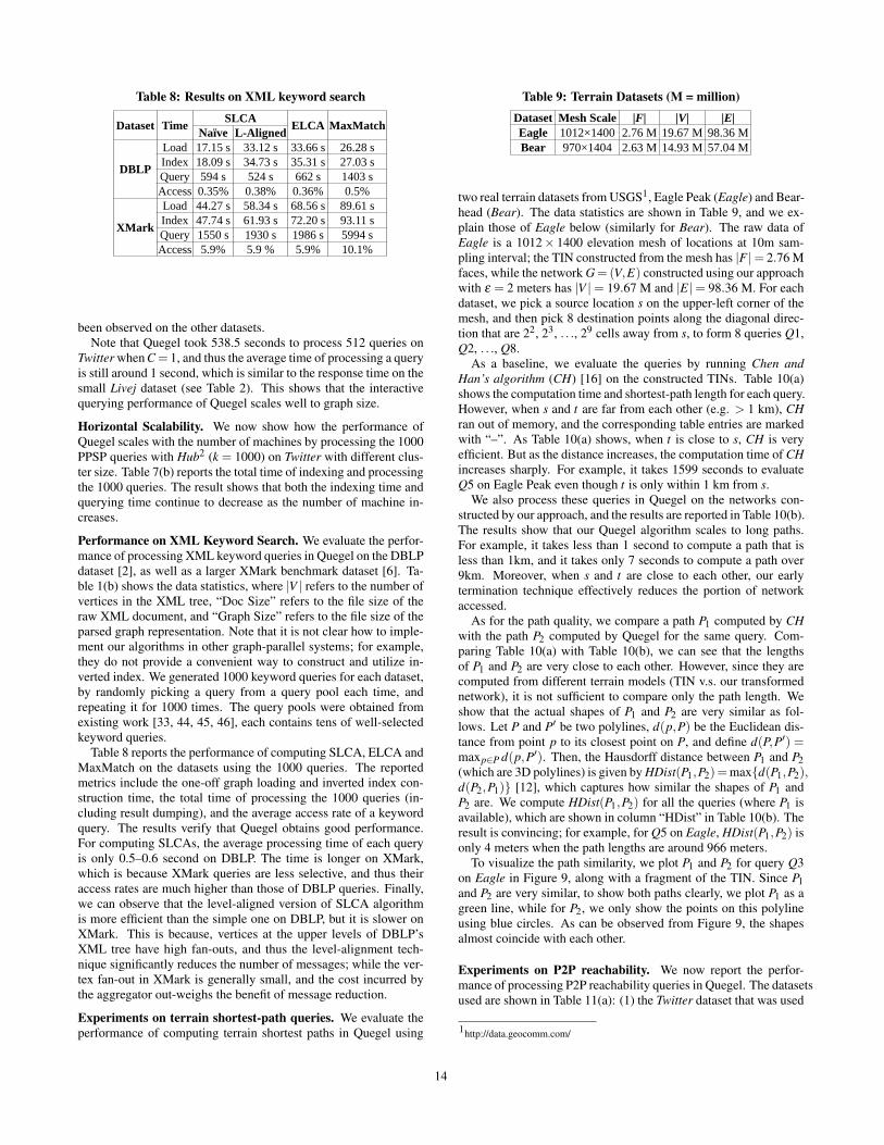
Table 8: Results on XML keyword search

Dataset Time SLCA ELCA MaxMatchNaïve L-Aligned

DBLP

Load 17.15 s 33.12 s 33.66 s 26.28 sIndex 18.09 s 34.73 s 35.31 s 27.03 sQuery 594 s 524 s 662 s 1403 sAccess 0.35% 0.38% 0.36% 0.5%

XMark

Load 44.27 s 58.34 s 68.56 s 89.61 sIndex 47.74 s 61.93 s 72.20 s 93.11 sQuery 1550 s 1930 s 1986 s 5994 sAccess 5.9% 5.9 % 5.9% 10.1%

been observed on the other datasets.Note that Quegel took 538.5 seconds to process 512 queries on

Twitter when C = 1, and thus the average time of processing a queryis still around 1 second, which is similar to the response time on thesmall Livej dataset (see Table 2). This shows that the interactivequerying performance of Quegel scales well to graph size.

Horizontal Scalability. We now show how the performance ofQuegel scales with the number of machines by processing the 1000PPSP queries with Hub2 (k = 1000) on Twitter with different clus-ter size. Table 7(b) reports the total time of indexing and processingthe 1000 queries. The result shows that both the indexing time andquerying time continue to decrease as the number of machine in-creases.

Performance on XML Keyword Search. We evaluate the perfor-mance of processing XML keyword queries in Quegel on the DBLPdataset [2], as well as a larger XMark benchmark dataset [6]. Ta-ble 1(b) shows the data statistics, where |V | refers to the number ofvertices in the XML tree, “Doc Size” refers to the file size of theraw XML document, and “Graph Size” refers to the file size of theparsed graph representation. Note that it is not clear how to imple-ment our algorithms in other graph-parallel systems; for example,they do not provide a convenient way to construct and utilize in-verted index. We generated 1000 keyword queries for each dataset,by randomly picking a query from a query pool each time, andrepeating it for 1000 times. The query pools were obtained fromexisting work [33, 44, 45, 46], each contains tens of well-selectedkeyword queries.

Table 8 reports the performance of computing SLCA, ELCA andMaxMatch on the datasets using the 1000 queries. The reportedmetrics include the one-off graph loading and inverted index con-struction time, the total time of processing the 1000 queries (in-cluding result dumping), and the average access rate of a keywordquery. The results verify that Quegel obtains good performance.For computing SLCAs, the average processing time of each queryis only 0.5–0.6 second on DBLP. The time is longer on XMark,which is because XMark queries are less selective, and thus theiraccess rates are much higher than those of DBLP queries. Finally,we can observe that the level-aligned version of SLCA algorithmis more efficient than the simple one on DBLP, but it is slower onXMark. This is because, vertices at the upper levels of DBLP’sXML tree have high fan-outs, and thus the level-alignment tech-nique significantly reduces the number of messages; while the ver-tex fan-out in XMark is generally small, and the cost incurred bythe aggregator out-weighs the benefit of message reduction.

Experiments on terrain shortest-path queries. We evaluate theperformance of computing terrain shortest paths in Quegel using

Table 9: Terrain Datasets (M = million)Dataset Mesh Scale |F| |V| |E|Eagle 1012×1400 2.76 M 19.67 M 98.36 MBear 970×1404 2.63 M 14.93 M 57.04 M

two real terrain datasets from USGS1, Eagle Peak (Eagle) and Bear-head (Bear). The data statistics are shown in Table 9, and we ex-plain those of Eagle below (similarly for Bear). The raw data ofEagle is a 1012× 1400 elevation mesh of locations at 10m sam-pling interval; the TIN constructed from the mesh has |F |= 2.76 Mfaces, while the network G= (V,E) constructed using our approachwith ε = 2 meters has |V |= 19.67 M and |E|= 98.36 M. For eachdataset, we pick a source location s on the upper-left corner of themesh, and then pick 8 destination points along the diagonal direc-tion that are 22, 23, . . ., 29 cells away from s, to form 8 queries Q1,Q2, . . ., Q8.

As a baseline, we evaluate the queries by running Chen andHan’s algorithm (CH) [16] on the constructed TINs. Table 10(a)shows the computation time and shortest-path length for each query.However, when s and t are far from each other (e.g. > 1 km), CHran out of memory, and the corresponding table entries are markedwith “–”. As Table 10(a) shows, when t is close to s, CH is veryefficient. But as the distance increases, the computation time of CHincreases sharply. For example, it takes 1599 seconds to evaluateQ5 on Eagle Peak even though t is only within 1 km from s.

We also process these queries in Quegel on the networks con-structed by our approach, and the results are reported in Table 10(b).The results show that our Quegel algorithm scales to long paths.For example, it takes less than 1 second to compute a path that isless than 1km, and it takes only 7 seconds to compute a path over9km. Moreover, when s and t are close to each other, our earlytermination technique effectively reduces the portion of networkaccessed.

As for the path quality, we compare a path P1 computed by CHwith the path P2 computed by Quegel for the same query. Com-paring Table 10(a) with Table 10(b), we can see that the lengthsof P1 and P2 are very close to each other. However, since they arecomputed from different terrain models (TIN v.s. our transformednetwork), it is not sufficient to compare only the path length. Weshow that the actual shapes of P1 and P2 are very similar as fol-lows. Let P and P′ be two polylines, d(p,P) be the Euclidean dis-tance from point p to its closest point on P, and define d(P,P′) =maxp∈P d(p,P′). Then, the Hausdorff distance between P1 and P2(which are 3D polylines) is given by HDist(P1,P2)=max{d(P1,P2),d(P2,P1)} [12], which captures how similar the shapes of P1 andP2 are. We compute HDist(P1,P2) for all the queries (where P1 isavailable), which are shown in column “HDist” in Table 10(b). Theresult is convincing; for example, for Q5 on Eagle, HDist(P1,P2) isonly 4 meters when the path lengths are around 966 meters.

To visualize the path similarity, we plot P1 and P2 for query Q3on Eagle in Figure 9, along with a fragment of the TIN. Since P1and P2 are very similar, to show both paths clearly, we plot P1 as agreen line, while for P2, we only show the points on this polylineusing blue circles. As can be observed from Figure 9, the shapesalmost coincide with each other.

Experiments on P2P reachability. We now report the perfor-mance of processing P2P reachability queries in Quegel. The datasetsused are shown in Table 11(a): (1) the Twitter dataset that was used

1http://data.geocomm.com/

14

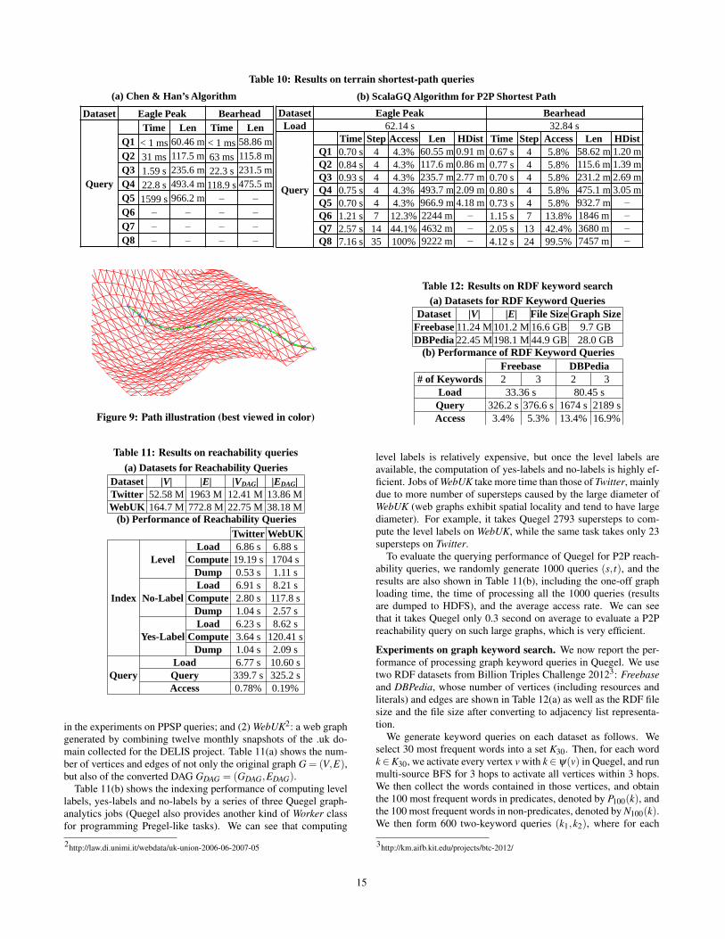
Table 10: Results on terrain shortest-path queries

Dataset Eagle Peak BearheadLoad 62.14 s 32.84 s

Query

Time Step Access Len HDist Time Step Access Len HDistQ1 0.70 s 4 4.3% 60.55 m 0.91 m 0.67 s 4 5.8% 58.62 m 1.20 mQ2 0.84 s 4 4.3% 117.6 m 0.86 m 0.77 s 4 5.8% 115.6 m 1.39 mQ3 0.93 s 4 4.3% 235.7 m 2.77 m 0.70 s 4 5.8% 231.2 m 2.69 mQ4 0.75 s 4 4.3% 493.7 m 2.09 m 0.80 s 4 5.8% 475.1 m 3.05 mQ5 0.70 s 4 4.3% 966.9 m 4.18 m 0.73 s 4 5.8% 932.7 m −Q6 1.21 s 7 12.3% 2244 m − 1.15 s 7 13.8% 1846 m −Q7 2.57 s 14 44.1% 4632 m − 2.05 s 13 42.4% 3680 m −Q8 7.16 s 35 100% 9222 m − 4.12 s 24 99.5% 7457 m −

Dataset Eagle Peak Bearhead

Query

Time Len Time LenQ1 < 1 ms 60.46 m < 1 ms 58.86 mQ2 31 ms 117.5 m 63 ms 115.8 mQ3 1.59 s 235.6 m 22.3 s 231.5 mQ4 22.8 s 493.4 m 118.9 s 475.5 mQ5 1599 s 966.2 m − −Q6 − − − −Q7 − − − −Q8 − − − −

(a) Chen & Han’s Algorithm (b) ScalaGQ Algorithm for P2P Shortest Path

Figure 9: Path illustration (best viewed in color)

Table 11: Results on reachability queries

Dataset |V| |E| |VDAG| |EDAG|Twitter 52.58 M 1963 M 12.41 M 13.86 MWebUK 164.7 M 772.8 M 22.75 M 38.18 M

(a) Datasets for Reachability Queries

Twitter WebUK

Index

LevelLoad 6.86 s 6.88 s

Compute 19.19 s 1704 sDump 0.53 s 1.11 s

No-LabelLoad 6.91 s 8.21 s

Compute 2.80 s 117.8 sDump 1.04 s 2.57 s

Yes-LabelLoad 6.23 s 8.62 s

Compute 3.64 s 120.41 sDump 1.04 s 2.09 s

QueryLoad 6.77 s 10.60 s

Query 339.7 s 325.2 sAccess 0.78% 0.19%

(b) Performance of Reachability Queries

in the experiments on PPSP queries; and (2) WebUK2: a web graphgenerated by combining twelve monthly snapshots of the .uk do-main collected for the DELIS project. Table 11(a) shows the num-ber of vertices and edges of not only the original graph G = (V,E),but also of the converted DAG GDAG = (GDAG,EDAG).

Table 11(b) shows the indexing performance of computing levellabels, yes-labels and no-labels by a series of three Quegel graph-analytics jobs (Quegel also provides another kind of Worker classfor programming Pregel-like tasks). We can see that computing

2http://law.di.unimi.it/webdata/uk-union-2006-06-2007-05

Table 12: Results on RDF keyword search

Dataset |V| |E| File Size Graph SizeFreebase 11.24 M 101.2 M 16.6 GB 9.7 GBDBPedia 22.45 M198.1 M 44.9 GB 28.0 GB

(a) Datasets for RDF Keyword Queries

(b) Performance of RDF Keyword QueriesFreebase DBPedia

# of Keywords 2 3 2 3Load 33.36 s 80.45 s

Query 326.2 s 376.6 s 1674 s 2189 sAccess 3.4% 5.3% 13.4% 16.9%

level labels is relatively expensive, but once the level labels areavailable, the computation of yes-labels and no-labels is highly ef-ficient. Jobs of WebUK take more time than those of Twitter, mainlydue to more number of supersteps caused by the large diameter ofWebUK (web graphs exhibit spatial locality and tend to have largediameter). For example, it takes Quegel 2793 supersteps to com-pute the level labels on WebUK, while the same task takes only 23supersteps on Twitter.

To evaluate the querying performance of Quegel for P2P reach-ability queries, we randomly generate 1000 queries (s, t), and theresults are also shown in Table 11(b), including the one-off graphloading time, the time of processing all the 1000 queries (resultsare dumped to HDFS), and the average access rate. We can seethat it takes Quegel only 0.3 second on average to evaluate a P2Preachability query on such large graphs, which is very efficient.

Experiments on graph keyword search. We now report the per-formance of processing graph keyword queries in Quegel. We usetwo RDF datasets from Billion Triples Challenge 20123: Freebaseand DBPedia, whose number of vertices (including resources andliterals) and edges are shown in Table 12(a) as well as the RDF filesize and the file size after converting to adjacency list representa-tion.

We generate keyword queries on each dataset as follows. Weselect 30 most frequent words into a set K30. Then, for each wordk∈K30, we activate every vertex v with k∈ψ(v) in Quegel, and runmulti-source BFS for 3 hops to activate all vertices within 3 hops.We then collect the words contained in those vertices, and obtainthe 100 most frequent words in predicates, denoted by P100(k), andthe 100 most frequent words in non-predicates, denoted by N100(k).We then form 600 two-keyword queries (k1,k2), where for each

3http://km.aifb.kit.edu/projects/btc-2012/

15

k1 ∈ K30 we randomly select 20 words k2 ∈ N100(k1); and form600 three-keyword queries (k1,k2,k3), where for each k1 ∈K30, werandomly select 20 word pairs (k2,k3) with k2 ∈ P100(k1) and k3 ∈N100(k1). We generate queries in this way, so that k1 has relativelylow selectivity while k2 and k3 are also relevant to k1.

Table 12(b) reports the performance of processing the graph key-word queries, including the one-off graph loading time, the totalprocessing time of all 600 queries, and the average access rate. Wecan see that it takes Quegel only 0.3 second on average to evaluatea graph keyword query on Freebase and 1–2 seconds on averageon DBPedia, which is very efficient given the big data size. More-over, the querying time and access rate are higher when there are 3keywords in the query, which shows that the query cost generallyincreases with the number of keywords in a query.

7. CONCLUSIONSWe developed a distributed system, Quegel, for general-purpose

querying of big graphs. To our knowledge, this is the first work thatstudies how to apply Pregel’s user-friendly vertex-centric program-ming interface to efficiently process queries in big graphs. This isalso the first general-purpose system that applies graph indexing tospeed up query processing in a distributed platform. We demon-strated how Quegel is used to process five types of queries, i.e.,PPSP queries, XML keyword queries, terrain shortest path queries,point-to-point reachability queries, and graph keyword queries. Wealso showed Quegel obtained good performance for processing thesequeries.

For future work, we will continue to improve the performanceof Quegel by designing various optimization techniques, propos-ing efficient graph indexes to be adopted in Quegel, and provid-ing performance guarantees for answering different types of graphqueries [37].

8. REFERENCES[1] Apache Giraph: http://giraph.apache.org.[2] http://dblp.uni-trier.de/xml/.[3] http://km.aifb.kit.edu/projects/btc-2009.[4] http://konect.uni-koblenz.de/networks/

livejournal-groupmemberships.[5] http:

//konect.uni-koblenz.de/networks/twitter_mpi.[6] http://www.xml-benchmark.org/.[7] J. Cheng, J. X. Yu, B. Ding, P. S. Yu, and H. Wang. Fast graph

pattern matching. In ICDE, pages 913–922, 2008.[8] J. Gao, C. Zhou, J. Zhou, and J. X. Yu. Continuous pattern detection

over billion-edge graph using distributed framework. In ICDE, pages556–567, 2014.

[9] J. E. Gonzalez, Y. Low, H. Gu, D. Bickson, and C. Guestrin.Powergraph: Distributed graph-parallel computation on naturalgraphs. In OSDI, pages 17–30, 2012.

[10] J. E. Gonzalez, R. S. Xin, A. Dave, D. Crankshaw, M. J. Franklin,and I. Stoica. Graphx: Graph processing in a distributed dataflowframework. In OSDI, 2014.

[11] M. Han, K. Daudjee, K. Ammar, M. T. Ozsu, X. Wang, and T. Jin.An experimental comparison of Pregel-like graph processingsystems. PVLDB, 7(12):1047–1058, 2014.

[12] J. Hangouet. Computation of the Hausdorff distance between planevector polylines. In AUTO-CARTO, pages 1–10, 1995.

[13] H. He, H. Wang, J. Yang, and P. S. Yu. BLINKS: ranked keywordsearches on graphs. In SIGMOD, pages 305–316, 2007.

[14] B. Iordanov. HyperGraphDB: A generalized graph database. InWAIM Workshop on Graph Database, pages 25–36, 2010.

[15] R. Jin, N. Ruan, B. You, and H. Wang. Hub-accelerator: Fast andexact shortest path computation in large social networks. CoRR,abs/1305.0507, 2013.

[16] B. Kaneva and J. O’Rourke. An implementation of Chen & Han’sshortest paths algorithm. In Proceedings of the 12th CanadianConference on Computational Geometry, 2000.

[17] M. Kaul, R. C. Wong, B. Yang, and C. S. Jensen. Finding shortestpaths on terrains by killing two birds with one stone. PVLDB,7(1):73–84, 2013.

[18] A. Khan and S. Elnikety. Systems for big-graphs. PVLDB,7(13):1709–1710, 2014.

[19] A. Kyrola, G. E. Blelloch, and C. Guestrin. GraphChi: Large-scalegraph computation on just a PC. In OSDI, pages 31–46, 2012.

[20] L. Liu and R. C. Wong. Finding shortest path on land surface. InSIGMOD, pages 433–444, 2011.

[21] Z. Liu and Y. Chen. Reasoning and identifying relevant matches forXML keyword search. PVLDB, 1(1):921–932, 2008.

[22] Y. Low, J. Gonzalez, A. Kyrola, D. Bickson, C. Guestrin, and J. M.Hellerstein. Distributed GraphLab: A framework for machinelearning in the cloud. PVLDB, 5(8):716–727, 2012.

[23] Y. Lu, J. Cheng, D. Yan, and H. Wu. Large-scale distributed graphcomputing systems: An experimental evaluation. PVLDB,8(3):281–292, 2014.

[24] G. Malewicz, M. H. Austern, A. J. C. Bik, J. C. Dehnert, I. Horn,N. Leiser, and G. Czajkowski. Pregel: a system for large-scale graphprocessing. In SIGMOD Conference, pages 135–146, 2010.

[25] Neo Technology. Neo4j graph database. http://www.neo4j.org/.[26] L. Qin, J. X. Yu, L. Chang, H. Cheng, C. Zhang, and X. Lin. Scalable

big graph processing in mapreduce. In SIGMOD, pages 827–838,2014.

[27] A. Roy, I. Mihailovic, and W. Zwaenepoel. X-stream: edge-centricgraph processing using streaming partitions. In SOSP, pages472–488, 2013.

[28] S. Sakr, S. Elnikety, and Y. He. G-SPARQL: a hybrid engine forquerying large attributed graphs. In CIKM, pages 335–344, 2012.

[29] S. Salihoglu and J. Widom. GPS: a graph processing system. InSSDBM, page 22, 2013.

[30] M. Sarwat, S. Elnikety, Y. He, and M. F. Mokbel. Horton+: Adistributed system for processing declarative reachability queriesover partitioned graphs. PVLDB, 6(14):1918–1929, 2013.

[31] C. Shahabi, L. A. Tang, and S. Xing. Indexing land surface forefficient knn query. PVLDB, 1(1):1020–1031, 2008.

[32] B. Shao, H. Wang, and Y. Li. Trinity: a distributed graph engine on amemory cloud. In SIGMOD, pages 505–516, 2013.

[33] A. Termehchy and M. Winslett. Using structural information in XMLkeyword search effectively. ACM Trans. Database Syst., 36(1):4,2011.

[34] H. Wei, J. X. Yu, C. Lu, and R. Jin. Reachability querying: Anindependent permutation labeling approach. PVLDB,7(12):1191–1202, 2014.

[35] D. Yan, J. Cheng, Y. Lu, and W. Ng. Blogel: A block-centricframework for distributed computation on real-world graphs.PVLDB, 7(14):1981–1992, 2014.

[36] D. Yan, J. Cheng, Y. Lu, and W. Ng. Effective techniques formessage reduction and load balancing in distributed graphcomputation. In WWW, pages 1307–1317, 2015.

[37] D. Yan, J. Cheng, K. Xing, Y. Lu, W. Ng, and Y. Bu. Pregelalgorithms for graph connectivity problems with performanceguarantees. PVLDB, 7(14):1821–1832, 2014.

[38] D. Yan, Z. Zhao, and W. Ng. Monochromatic and bichromaticreverse nearest neighbor queries on land surfaces. In CIKM, pages942–951, 2012.

[39] D. Yang, D. Zhang, K. Tan, J. Cao, and F. L. Mouel. CANDS:continuous optimal navigation via distributed stream processing.PVLDB, 8(2):137–148, 2014.

[40] F. Yang, J. Li, and J. Cheng. Husky: Towards a more efficient andexpressive distributed computing framework. PVLDB, 9(5):420–431,2016.

[41] C. Zhang, Q. Ma, X. Wang, and A. Zhou. Distributed SLCA-basedXML keyword search by map-reduce. In DASFAA Workshop onUbiquitous Data Management, pages 386–397, 2010.

[42] Z. Zhang, J. X. Yu, L. Qin, and Z. Shang. Divide & conquer: I/Oefficient depth-first search. In SIGMOD, pages 445–458, 2015.

16

[43] Z. Zhang, J. X. Yu, L. Qin, Q. Zhu, and X. Zhou. I/O costminimization: reachability queries processing over massive graphs.In EDBT, pages 468–479, 2012.

[44] J. Zhou, Z. Bao, Z. Chen, and T. W. Ling. Fast result enumeration forkeyword queries on XML data. In DASFAA, pages 95–109, 2012.

[45] J. Zhou, Z. Bao, W. Wang, T. W. Ling, Z. Chen, X. Lin, and J. Guo.Fast SLCA and ELCA computation for XML keyword queries basedon set intersection. In ICDE, pages 905–916, 2012.

[46] J. Zhou, Z. Bao, W. Wang, J. Zhao, and X. Meng. Efficient queryprocessing for XML keyword queries based on the idlist index.VLDB J., 23(1):25–50, 2014.

17