Quaternion Algebraic Geometry

Dominic Widdows

June 5, 2006

Abstract

QUATERNION ALGEBRAIC GEOMETRY

DOMINIC WIDDOWS

St Anne’s College, Oxford

Thesis submitted Hilary Term, 2000, in supportof application to supplicate for the degree of D.Phil.

This thesis is a collection of results about hypercomplex and quaternionic manifolds,focussing on two main areas. These are exterior forms and double complexes, and the‘algebraic geometry’ of hypercomplex manifolds. The latter area is strongly influencedby techniques from quaternionic algebra.

A new double complex on quaternionic manifolds is presented, a quaternionic versionof the Dolbeault complex on a complex manifold. It arises from the decomposition ofreal-valued exterior forms on a quaternionic manifold M into irreducible representationsof Sp(1). This decomposition gives a double complex of differential forms and operatorsas a result of the Clebsch-Gordon formula Vr⊗V1

∼= Vr+1⊕Vr−1 for Sp(1)-representations.The properties of the double complex are investigated, and it is established that it iselliptic in most places.

Joyce has created a new theory of quaternionic algebra [J1] by defining a quaternionictensor product for AH-modules (H-modules equipped with a special real subspace). Thetheory can be described using sheaves over CP 1, an interpretation due to Quillen [Q].AH-modules and their quaternionic tensor products are classified. Stable AH-modulesare described using Sp(1)-representations.

This theory is especially useful for describing hypercomplex manifolds and formingclose analogies with complex geometry. Joyce has defined and investigated q-holomorphicfunctions on hypercomplex manifolds. There is also a q-holomorphic cotangent spacewhich again arises as a result of the Clebsch-Gordon formula. AH-module bundles aredefined and their q-holomorphic sections explored.

Quaternion-valued differential forms on hypercomplex manifolds are of special inter-est. Their decomposition is finer than that of real forms, giving a second double complexwith special advantages. The cohomology of these complexes leads to new invariants ofcompact quaternionic and hypercomplex manifolds.

Quaternion-valued vector fields are also studied, and lead to the definition of quater-nionic Lie algebras. The investigation of finite-dimensional quaternionic Lie algebrasallows the calculation of some simple quaternionic cohomology groups.

Acknowledgements

I would like to express gratitude, appreciation and respect for my supervisor Do-minic Joyce. Without his inspiration as a mathematician this thesis would not havebeen conceived; without his patience and friendship it would certainly not have beencompleted.

Dedication

To the memory of Dr Peter Rowe, 1938-1998, who taught me relativity as anundergraduate in Durham. His determination to teach concepts before examination

techniques introduced me to differential geometry.

i

Contents

Introduction 1

1 The Quaternions and the Group Sp(1) 41.1 The Quaternions . . . . . . . . . . . . . . . . . . . . . . . . . . . . . . . 41.2 The Lie Group Sp(1) and its Representations . . . . . . . . . . . . . . . 91.3 Difficulties with the Quaternions . . . . . . . . . . . . . . . . . . . . . . . 12

2 Quaternionic Differential Geometry 172.1 Complex, Hypercomplex and Quaternionic Manifolds . . . . . . . . . . . 172.2 Differential Forms on Complex Manifolds . . . . . . . . . . . . . . . . . . 202.3 Differential Forms on Quaternionic Manifolds . . . . . . . . . . . . . . . 23

3 A Double Complex on Quaternionic Manifolds 253.1 Real forms on Complex Manifolds . . . . . . . . . . . . . . . . . . . . . . 253.2 Construction of the Double Complex . . . . . . . . . . . . . . . . . . . . 283.3 Ellipticity and the Double Complex . . . . . . . . . . . . . . . . . . . . . 323.4 Quaternion-valued forms on Hypercomplex Manifolds . . . . . . . . . . . 40

4 Developments in Quaternionic Algebra 424.1 The Quaternionic Algebra of Joyce . . . . . . . . . . . . . . . . . . . . . 424.2 Duality in Quaternionic Algebra . . . . . . . . . . . . . . . . . . . . . . . 484.3 Real Subspaces of Complex Vector Spaces . . . . . . . . . . . . . . . . . 524.4 K-modules . . . . . . . . . . . . . . . . . . . . . . . . . . . . . . . . . . . 534.5 The Sheaf-Theoretic approach of Quillen . . . . . . . . . . . . . . . . . . 56

5 Quaternionic Algebra and Sp(1)-representations 615.1 Stable AH-modules and Sp(1)-representations . . . . . . . . . . . . . . . 615.2 Sp(1)-Representations and the Quaternionic Tensor Product . . . . . . . 685.3 Semistable AH-modules and Sp(1)-representations . . . . . . . . . . . . . 745.4 Examples and Summary of AH-modules . . . . . . . . . . . . . . . . . . 77

6 Hypercomplex Manifolds 806.1 Q-holomorphic Functions and H-algebras . . . . . . . . . . . . . . . . . . 816.2 The Quaternionic Cotangent Space . . . . . . . . . . . . . . . . . . . . . 866.3 AH-bundles . . . . . . . . . . . . . . . . . . . . . . . . . . . . . . . . . . 906.4 Q-holomorphic AH-bundles . . . . . . . . . . . . . . . . . . . . . . . . . 93

ii

7 Quaternion Valued Forms and Vector Fields 1007.1 The Quaternion-valued Double Complex . . . . . . . . . . . . . . . . . . 1017.2 Vector Fields and Quaternionic Lie Algebras . . . . . . . . . . . . . . . . 1097.3 Hypercomplex Lie groups . . . . . . . . . . . . . . . . . . . . . . . . . . 112

References 117

iii

Introduction

This aim of this thesis is to describe and develop various aspects of quaternionic algebraand geometry. The approach is based upon two pillars, namely the differential geometryof quaternionic manifolds and Joyce’s recent theory of quaternionic algebra. Contribu-tions are made to both fields of study, enabling these strands to be woven together indescribing the algebraic geometry of hypercomplex manifolds.

A recurrent theme throughout will be representations of the group Sp(1) of unitquaternions. Our contribution to the theory of quaternionic manifolds relies on decom-posing the Sp(1)-action on exterior forms, whilst the main new insight in quaternionicalgebra is that the most important building blocks of Joyce’s theory are best describedand manipulated as Sp(1)-representations. The importance of Sp(1)-representations toboth areas is chiefly responsible for the successful synthesis of methods in the work onhypercomplex manifolds.

Another frequent source of motivation is the behaviour of the complex numbers.Many situations in complex algebra and geometry have interesting quaternionic ana-logues. Aspects of complex geometry can often be described using the group U(1) of unitcomplex numbers; replacing this with the group Sp(1) can lead directly to quaternionicversions. The decomposition of exterior forms on quaternionic manifolds is preciselysuch an example, as is all the work on q-holomorphic functions and forms on hypercom-plex manifolds. On the other hand, Joyce’s quaternionic algebra is such a rich theoryprecisely because real subspaces of quaternionic vector spaces behave so differently fromreal subspaces of complex vector spaces.

Much of the original work presented is enticingly simple — indeed, I have often feltboth surprised and privileged that it has not been carried out before. One of the mainexplanations for this is the relative unpopularity suffered by the quaternions in the 20th

century. This situation has left various aspects of quaternionic behaviour unexplored.To help understand the reasons for this omission and the consequent opportunities fordevelopment, the first chapter is devoted to a survey of the history of the quaternionsand their applications. Background material also includes an introduction to the groupSp(1) and its representations. The irreducible representations on complex vector spacesand their tensor products are described, as are real and quaternionic representations.

Chapter 2 is about quaternionic structures in differential geometry. The approachis based on the work of Salamon [S3]. Taking complex manifolds as a model, hyper-complex manifolds (those possessing a torsion-free GL(n,H)-structure) are defined, fol-lowed by the broader class of quaternionic manifolds (those possessing a torsion-freeSp(1)GL(n,H)-structure). After reviewing the Dolbeault complex, we consider thedecomposition of differential forms on quaternionic manifolds, including an importantelliptic complex discovered by Salamon upon which the integrability of the quaternionic

1

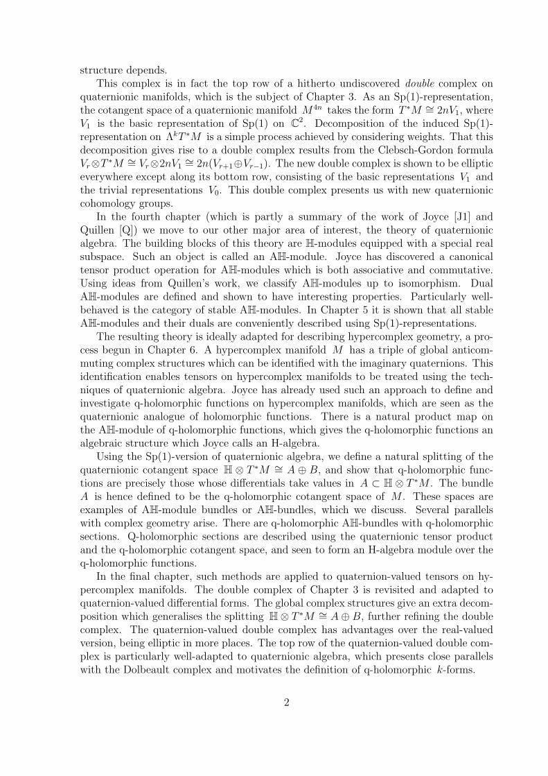
structure depends.This complex is in fact the top row of a hitherto undiscovered double complex on

quaternionic manifolds, which is the subject of Chapter 3. As an Sp(1)-representation,the cotangent space of a quaternionic manifold M4n takes the form T ∗M ∼= 2nV1, whereV1 is the basic representation of Sp(1) on C2. Decomposition of the induced Sp(1)-representation on ΛkT ∗M is a simple process achieved by considering weights. That thisdecomposition gives rise to a double complex results from the Clebsch-Gordon formulaVr⊗T ∗M ∼= Vr⊗2nV1

∼= 2n(Vr+1⊕Vr−1). The new double complex is shown to be ellipticeverywhere except along its bottom row, consisting of the basic representations V1 andthe trivial representations V0. This double complex presents us with new quaternioniccohomology groups.

In the fourth chapter (which is partly a summary of the work of Joyce [J1] andQuillen [Q]) we move to our other major area of interest, the theory of quaternionicalgebra. The building blocks of this theory are H-modules equipped with a special realsubspace. Such an object is called an AH-module. Joyce has discovered a canonicaltensor product operation for AH-modules which is both associative and commutative.Using ideas from Quillen’s work, we classify AH-modules up to isomorphism. DualAH-modules are defined and shown to have interesting properties. Particularly well-behaved is the category of stable AH-modules. In Chapter 5 it is shown that all stableAH-modules and their duals are conveniently described using Sp(1)-representations.

The resulting theory is ideally adapted for describing hypercomplex geometry, a pro-cess begun in Chapter 6. A hypercomplex manifold M has a triple of global anticom-muting complex structures which can be identified with the imaginary quaternions. Thisidentification enables tensors on hypercomplex manifolds to be treated using the tech-niques of quaternionic algebra. Joyce has already used such an approach to define andinvestigate q-holomorphic functions on hypercomplex manifolds, which are seen as thequaternionic analogue of holomorphic functions. There is a natural product map onthe AH-module of q-holomorphic functions, which gives the q-holomorphic functions analgebraic structure which Joyce calls an H-algebra.

Using the Sp(1)-version of quaternionic algebra, we define a natural splitting of thequaternionic cotangent space H ⊗ T ∗M ∼= A ⊕ B, and show that q-holomorphic func-tions are precisely those whose differentials take values in A ⊂ H ⊗ T ∗M . The bundleA is hence defined to be the q-holomorphic cotangent space of M . These spaces areexamples of AH-module bundles or AH-bundles, which we discuss. Several parallelswith complex geometry arise. There are q-holomorphic AH-bundles with q-holomorphicsections. Q-holomorphic sections are described using the quaternionic tensor productand the q-holomorphic cotangent space, and seen to form an H-algebra module over theq-holomorphic functions.

In the final chapter, such methods are applied to quaternion-valued tensors on hy-percomplex manifolds. The double complex of Chapter 3 is revisited and adapted toquaternion-valued differential forms. The global complex structures give an extra decom-position which generalises the splitting H⊗ T ∗M ∼= A⊕ B, further refining the doublecomplex. The quaternion-valued double complex has advantages over the real-valuedversion, being elliptic in more places. The top row of the quaternion-valued double com-plex is particularly well-adapted to quaternionic algebra, which presents close parallelswith the Dolbeault complex and motivates the definition of q-holomorphic k-forms.

2

Quaternion-valued vector fields are also interesting. The quaternionic tangent spacesplits as H⊗TM ∼= A⊕ B in the same way as the cotangent space. Vector fields takingvalues in A are closed under the quaternionic tensor product and Lie bracket, a resultwhich depends upon the integrability of the hypercomplex structure. This is the quater-nionic analogue of the statement that on a complex manifold, the (1, 0) vector fields areclosed under the Lie bracket. The vector fields in question therefore form a quaternionicLie algebra, a new concept which we introduce. Interesting finite-dimensional quater-nionic Lie algebras are used to calculate some quaternionic cohomology groups on Liegroups with left-invariant hypercomplex structures.

3

Chapter 1

The Quaternions and the GroupSp(1)

1.1 The Quaternions

The quaternions H are a four-dimensional real algebra generated by the identity element 1and the symbols i1, i2 and i3, so H = r0+r1i1+r2i2+r3i3 : r0, . . . , r3 ∈ R. Quaternionsare added together component by component, and quaternion multiplication is given bythe quaternion relations

i1i2 = −i2i1 = i3, i2i3 = −i3i2 = i1, i3i1 = −i1i3 = i2, i21 = i22 = i23 = −1 (1.1)

and the distributive law. The quaternion algebra is not commutative, though it doesobey the associative law. The quaternions are a division algebra (an algebra with theproperty that ab = 0 implies that a = 0 or b = 0 ).

• Define the imaginary quaternions I = 〈i1, i2, i3〉. The symbol I is not standard,but we will use it throughout.

• Define the conjugate q of q = q0 + q1i1 + q2i2 + q3i3 by q = q0 − q1i1 − q2i2 − q3i3.Then (pq) = qp for all p, q ∈ H.

• Define the real and imaginary parts of q by Re(q) = q0 ∈ R and Im(q) = q1i1 +q2i2 + q3i3 ∈ I. As with complex numbers, q = Re(q)− Im(q).

• We regard the real numbers R as a subfield of H, and the quaternions as a directsum H ∼= R⊕ I.

• Let q = q1i1 + q2i2 + q3i3 ∈ I. Then q2 = −1 if and only if q21 + q2

2 + q23 = 1, so

the set of ‘quaternionic square-roots of minus-one’ is naturally isomorphic to the2-sphere S2. We shall often identify these sets, writing ‘q ∈ S2’ as a shorthand for‘q ∈ H : q2 = −1’.

• If q ∈ S2 then 〈1, q〉 is a subfield of H isomorphic to C. We shall call this subfieldCq.

4

1.1.1 A History of the Quaternions

The quaternions were discovered by the Irish mathematician and physicist, WilliamRowan Hamilton (1805-1865), 1 whose contributions to mechanics are well-known andwidely used. By 1835 Hamilton had helped to win acceptance for the system of complexnumbers by showing that calculations with complex numbers are equivalent to calcula-tions with ordered pairs of real numbers, governed by certain rules. At the time, complexnumbers were being applied very effectively to problems in the plane R2. To Hamilton,the next logical step was to seek a similar 3-dimensional number system which wouldrevolutionise calculations in R3. For years, he struggled with this problem. In a touchingletter to his son [H1], 2 dated shortly before his death in 1865, Hamilton writes:

Every morning, on my coming down to breakfast, your brother and yourselfused to ask me: “Well, Papa, can you multiply triplets?” Whereto I wasalways obliged to reply, with a sad shake of the head, “No, I can only addand subtract them”.

For several years, Hamilton tried to manipulate the three symbols 1, i and j into analgebra. He finally realised that the secret was to introduce a fourth dimension. On 16thOctober, 1843, whilst walking with his wife, he had a flash of inspiration. In the sameletter, he writes:

An electric circuit seemed to close, and a spark flashed forth, the herald(as I foresaw immediately) of many long years to come of definitely directedthought and work ... I pulled out on the spot a pocket-book, which stillexists, and made an entry there and then. Nor could I resist the impulse —unphilosophical as it may have been — to cut with a knife on the stone ofBrougham Bridge, as we passed it, the fundamental formula with the symbolsi, j, k:

i2 = j2 = k2 = ijk = −1,

which contains the solution of the problem, but of course, as an inscription,has long since mouldered away.

Substituting i1, i2, i3 for i, j, k, this gives the quaternion relations (1.1).Rarely do we possess such a clear account of the genesis of a piece of mathematics.

Most mathematical theories are invented gradually, and only after years of developmentcan they be presented in a lecture course as a definitive set of axioms and results. Thequaternions, on the other hand, “started into life, or light, full grown, on the 16th ofOcober, 1843...” 3 “Less than an hour elapsed” before Hamilton obtained leave of theCouncil of the Royal Irish Academy to read a paper on quaternions. The next day,Hamilton wrote a detailed letter to his friend and fellow mathematician John T. Graves

1Letters suggest that both Euler and Gauss were aware of the quaternion relations (1.1), thoughneither of them published the disovery [EKR, p. 192].

2Copies of Hamilton’s most significant letters and papers concerning quaternions are currently avail-able on the internet at www.maths.tcd.ie/pub/HistMath/People/Hamilton

3Letter to Professor P.G.Tait, an excerpt of which can be found on the same website as [H1].

5

[H2], giving us a clear account of the train of research which led him to his breakthrough.The discovery was published within a month on the 13th of November [H3].

The timing of the discovery amplified its impact upon Hamilton and his followers.The only other algebras known in 1843 were the real and complex numbers, both ofwhich can be regarded as subalgebras of the quaternions. (It was not until 1858 thatCayley introduced matrices, and showed that the quaternion algebra could be realisedas a subalgebra of the complex-valued 2 × 2 matrices.) As a result, Hamilton becamethe figurehead of a school of ‘quaternionists’, whose fervour for the new numbers farexceeded their usefulness. Hamilton believed his discovery to be of similar importanceto that of the infinitesimal calculus, and devoted the rest of his career exclusively to itsstudy. Echos of this zeal could still be heard this century; for example, while Eamonde Valera was President of Ireland (from 1959 to 1973), he would attend mathematicalmeetings whenever their title contained the word ‘quaternions’ !

Such excesses were bound to provoke a reaction, especially as it became clear thatthe quaternions are just one example of a number of possible algebras. Lord Kelvin, thefamous Scottish physicist, once remarked that “Quaternions came from Hamilton afterall his really good work had been done; and though beautifully ingenious, have been anunmixed evil to those who have touched them in any way” [EKR, p.193]. A belief thatquaternions are somehow obsolete is often tacitly accepted to this day.

This is far from the case. The quaternions remain the simplest algebra after thereal and complex numbers. Indeed, the real numbers R, the complex numbers C andthe quaternions H are the only associative division algebras, as was proved by GeorgFrobenius in 1878: and amongst these the quaternions are the most general. The dis-covery of the quaternions provided enormous stimulation to algebraic research and it isthought that the term ‘associative’ was coined by Hamilton himself [H3, p.5] to describequaternionic behaviour. Investigation into the nature of and constraints imposed byalgebraic properties such as associativity and commutativity was greatly accelerated bythe discovery of the quaternions.

The quaternions themselves have been used in various areas of mathematics. Mostrecently, quaternions have enjoyed prominence in computer science, because they are thesimplest algebraic tool for describing rotations in three and four dimensions. Certainly,the numbers have fallen short of the early expectations of the quaternionists. However,quaternions do shine a light on certain areas of mathematics, and those who becomefamiliar with them soon come to appreciate an intricacy and beauty which is all theirown.

1.1.2 Quaternions and Matrices

In this section we will make use of the older notation i = i1, j = i2, k = i3. This makesit easy to interpret i as the standard complex ‘square root of −1’ and j as a ‘structuremap’ on the complex vector space C2.

It is well-known that the quaternions can be written as real or complex matrices,because there are isomorphisms from H into subalgebras of Mat(4,R) and Mat(2,C).The former of these is given by the mapping

6

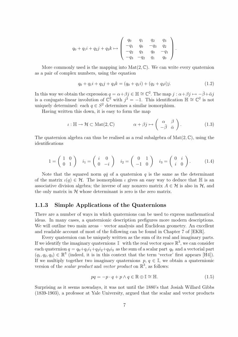
q0 + q1i+ q2j + q3k 7→

q0 q1 q2 q3−q1 q0 −q3 q2−q2 q3 q0 −q1−q3 −q2 q1 q0

.

More commonly used is the mapping into Mat(2,C). We can write every quaternionas a pair of complex numbers, using the equation

q0 + q1i+ q2j + q3k = (q0 + q1i) + (q2 + q3i)j. (1.2)

In this way we obtain the expression q = α+βj ∈ H ∼= C2. The map j : α+βj 7→ −β+αjis a conjugate-linear involution of C2 with j2 = −1. This identification H ∼= C2 is notuniquely determined: each q ∈ S2 determines a similar isomorphism.

Having written this down, it is easy to form the map

ι : H→ H ⊂ Mat(2,C) α+ βj 7→(

α β−β α

). (1.3)

The quaternion algebra can thus be realised as a real subalgebra of Mat(2,C), using theidentifications

1 =

(1 00 1

)i1 =

(i 00 −i

)i2 =

(0 1−1 0

)i3 =

(0 ii 0

). (1.4)

Note that the squared norm qq of a quaternion q is the same as the determinantof the matrix ι(q) ∈ H. The isomorphism ι gives an easy way to deduce that H is anassociative division algebra; the inverse of any nonzero matrix A ∈ H is also in H, andthe only matrix in H whose determinant is zero is the zero matrix.

1.1.3 Simple Applications of the Quaternions

There are a number of ways in which quaternions can be used to express mathematicalideas. In many cases, a quaternionic description prefigures more modern descriptions.We will outline two main areas – vector analysis and Euclidean geometry. An excellentand readable account of most of the following can be found in Chapter 7 of [EKR].

Every quaternion can be uniquely written as the sum of its real and imaginary parts.If we identify the imaginary quaternions I with the real vector space R3, we can considereach quaternion q = q0+q1i1+q2i2+q3i3 as the sum of a scalar part q0 and a vectorial part(q1, q2, q3) ∈ R3 (indeed, it is in this context that the term ‘vector’ first appears [H4]).If we multiply together two imaginary quaternions p, q ∈ I, we obtain a quaternionicversion of the scalar product and vector product on R3, as follows:

pq = −p · q + p ∧ q ∈ R⊕ I ∼= H. (1.5)

Surprising as it seems nowadays, it was not until the 1880’s that Josiah Willard Gibbs(1839-1903), a professor at Yale University, argued that the scalar and vector products

7

had their own meaning, independent from their quaternionic origins. It was he whointroduced the familiar notation p · q and p ∧ q — before his time these were written‘−Spq’ and ‘V pq’, indicating the ‘scalar’ and ‘vector’ parts of the quaternionic productpq ∈ H.

Another crucial part of vector analysis which originated with Hamilton and thequaternions is the ‘nabla’ operator ∇ (so-called by Hamilton because the symbol ∇is similar in shape to the Hebrew musical instrument of that name). The familiar gra-dient operator acting on a real differentiable function f(x1, x2, x3) : R3 → R was firstwritten as

∇f :=∂f

∂x1

i1 +∂f

∂x2

i2 +∂f

∂x3

i3. (1.6)

Hamilton went on to consider applying the operator ∇ to a ‘differentiable quaternionfield’ F (x1, x2, x3) = f1(x1, x2, x3)i1 + f2(x1, x2, x3)i2 + f3(x1, x2, x3)i3, obtaining theequation

∇F = −(∂f1

∂x1

+∂f2

∂x2

+∂f3

∂x3

)+

(∂f3

∂x2

− ∂f2

∂x3

)i1 +

(∂f1

∂x3

− ∂f3

∂x1

)i2 +

(∂f2

∂x1

− ∂f1

∂x2

)i3,

which we recognise in modern terminology as

∇F = − divF + curlF.

Applying the ∇ operator to Equation (1.6) leads to the well-known Laplacian operatoron R3:

∇2f = −(∂2f

∂x21

+∂2f

∂x22

+∂2f

∂x23

)=: ∆f.

Having obtained the standard scalar product on R3, we can obtain the Euclideanmetric on R4 in a similar fashion by relaxing the restriction in Equation (1.5) that pand q should be imaginary. For any p, q ∈ H, we have

Re(pq) = p0q0 + p1q1 + p2q2 + p3q3 ∈ R,

and so we define the canonical scalar product on H by

〈p, q〉 = Re(pq). (1.7)

We define the norm of a quaternion q ∈ H in the obvious way, putting

|q| =√qq. (1.8)

The norm function is multiplicative, i.e. |pq| = |p||q| for p, q ∈ H. As with complexnumbers, we can combine the norm function with conjugation to obtain the inverse ofq ∈ H \ 0 (it is easily verified that q−1 = q/|q|2 is the unique quaternion such thatqq−1 = q−1q = 1).

Another quaternionic formula, similar to Equation (1.7), is the identity

Re(pq) = p0q0 − p1q1 − p2q2 − p3q3 ∈ R. (1.9)

8

If we regard p and q as four-vectors in spacetime with the ‘time-axis’ identified withR ⊂ H and the ‘spatial part’ identified with I, this is identical to the Lorentz metric ofspecial relativity.

Let a and b be quaternions of unit norm, and consider the involution fa,b : H→ Hgiven by fa,b(q) = aqb. Then |fa,b(q)| = |q| and the function fa,b : R4 → R4 is a rotation.Clearly, f−a,−b = fa,b, so each of these choices for the pair a, b gives the same rotation.In 1855, Cayley showed that all rotations of R4 can be written in this fashion and thatthe two possibilities given above are the only two which give the same rotation. Also,all reflections can be obtained by the involutions fa,b(q) = aqb.

One of the beauties of this system is that having obtained all rotations of R4, weobtain the rotations of R3 simply by putting a = b−1, giving the inner automorphismof H, q 7→ aqa−1. (By Cayley’s theorem, all real-algebra automorphisms of H take thisform.) This fixes the real line R and rotates the imaginary quaternions I. Identifying Iwith R3, the map q 7→ aqa−1 is a rotation of R3. According to Cayley, within a yearof the discovery of the quaternions Hamilton was aware that all rotations of R3 can beexpressed in this fashion.

These discoveries provided much insight into the classical groups SO(3) and SO(4),and helped to develop our knowledge of transformation groups in general. There areinteresting questions which arise. Why do the unit quaternions turn out to be so im-portant? In view of the quaternionic version of the Lorentz metric in Equation (1.9),can we use quaternions to write Lorentz tranformations as elegantly? Are there otherspaces which might lend themselves to quaternionic treatment? These questions are bestaddressed using the theory of Lie groups, which the pioneering work of Hamilton andCayley helped to develop.

1.2 The Lie Group Sp(1) and its Representations

The unit quaternions form a subgroup of H under multiplication, which we call Sp(1).Its importance to the quaternions is equivalent to that of the circle group U(1) of unitcomplex numbers in complex analysis. As a manifold Sp(1) is the 3-sphere S3. Themultiplication and inverse maps are smooth, so Sp(1) is a compact Lie group. Theisomorphism ι : H→ H ⊂ Mat(2,C) of Equation (1.4) maps Sp(1) isomorphically ontoSU(2).

The Lie algebra sp(1) of Sp(1) is generated by the elements I, J and K, the Liebracket being given by the relations [I, J ] = 2K, [J,K] = 2I and [K, I] = 2J . We canwrite these using the matrices of Equation (1.4):

I =

(i 00 −i

)J =

(0 1−1 0

)K =

(0 ii 0

).

The complexification of sp(1) is the Lie algebra sl(2,C). This is generated over C bythe elements

H =

(1 00 −1

)X =

(0 10 0

)Y =

(0 01 0

), (1.10)

and the relations

[H,X] = 2X, [H, Y ] = −2Y and [X,Y ] = H. (1.11)

9

Hence the equations

I = iH, J = X − Y and K = i(X + Y ) (1.12)

give one possible identification sp(1)⊗R C ∼= sl(2,C).For any Q ∈ sp(1), the normaliser N(Q) of Q is defined to be

N(Q) = P ∈ sp(1) : [P,Q] = 0 = 〈Q〉,

which is a Cartan subalgebra of sp(1). Identifying a unit vector Q = aI+bJ+cK ∈ sp(1)with the corresponding imaginary quaternion q = ai2 + bi2 + ci3 ∈ S2, the exponentialmap exp : sp(1)→ Sp(1) maps 〈Q〉 to the unit circle in Cq, which we will call U(1)q.

In the previous section it was shown that rotations in three and four dimensions canbe written in terms of unit quaternions. This is because there is a commutative diagramof Lie group homomorphisms

Sp(1) ∼= Spin(3) → Sp(1)× Sp(1) ∼= Spin(4)

↓ ↓

SO(3) → SO(4).

(1.13)

The horizontal arrows are inclusions, and the vertical arrows are 2 : 1 coverings withkernels 1,−1 and (1, 1), (−1,−1) respectively. The applications of these homomor-phisms in Riemannian geometry are described by Salamon in [S1].

From this, we can see clearly why three- and four-dimensional Euclidean geometryfit so well in a quaternionic framework. We can also see why the same is not true forLorentzian geometry. Here the important group is the Lorentz group SO(3,1). Whilstthere is a double cover SL(2,C)→ SO0(3, 1), this does not restrict to a suitably interest-ing real homomorphism Sp(1)→ SO0(3,1). It is possible to write Lorentz transformationsusing quaternions (for a modern example see [dL]), but the author has found no waywhich is simple enough to be really effective. There have been attempts to use the bi-quaternions p + iq : p + q ∈ H ∼= H ⊗R C to apply quaternions to special relativity[Sy], but the mental gymnastics involved in using four ‘square roots of −1’ are cum-bersome: the equivalent description of ‘spin transformations’ using the matrices of thegroup SL(2,C) are a more familiar and fertile ground.

1.2.1 The Representations of Sp(1)

A representation of a Lie group G on a vector space V is a Lie group homomorphismρ : G→ GL(V ). We will sometimes refer to V itself as a representation where the mapρ is understood. The differential dρ is a Lie algebra representation dρ : g→ End(V ).

The representations of Sp(1) ∼= SU(2) will play an important part in this thesis.Their theory is well-known and used in many situations. Good introductions to Sp(1)-representations include [BD, §2.5] (which describes the action of the group SU(2)) and[FH, Lecture 11] (which provides a description in terms of the action of the Lie algebrasl(2,C)). We recall those points which will be of particular importance.

Because it is a compact group, every representation of Sp(1) on a complex vectorspace V can be written as a direct sum of irreducible representations. The multiplicity

10

of each irreducible in such a decomposition is uniquely determined. Moreover, there is aunique irreducible representation on Cn for every n > 0. This makes the representationsof Sp(1) particularly easy to describe. Let V1 be the basic representation of SL(2,C)on C2 given by left-action of matrices upon column vectors. This coincides with thebasic representation of Sp(1) by left-multiplication on H ∼= C2. The unique irreduciblerepresentation on Cn+1 is then given by the nth symmetric power of V1, so we define

Vn = Sn(V1).

The representation Vn is irreducible [BD, Proposition 5.1], and every irreducible rep-resentation of Sp(1) is of the form Vn for some nonnegative n ∈ Z [BD, Proposition5.3].

Let x and y be a basis for C2, so that V1 = 〈x,y〉. Then

Vn = Sn(V1) = 〈xn,xn−1y,xn−2y2, . . . ,x2yn−2,xyn−1,yn〉.

The action of SL(2,C) on Vn is given by the induced action on the space of homogeneouspolynomials of degree n in the variables x and y.

Each of the Lie group representations Vn is a representation of the Lie algebras sl(2,C)and sp(1). Another very important way to describe the structure of these representationsis obtained by decomposing them into weight spaces (eigenspaces for the action of aCartan subalgebra). In terms of H, X and Y , the sl(2,C)-action on V1 is given by

H(x) = x X(x) = 0 Y (x) = yH(y) = −y X(y) = x Y (y) = 0.

(1.14)

To obtain the induced action of sl(2,C) on Vn we use the Leibniz rule 4 A(a · b) =A(a) · b+ a · A(b). This gives

H(xn−kyk) = (n− 2k)(xn−kyk)

X(xn−kyk) = k(xn−k+1yk−1) (1.15)

Y (xn−kyk) = (n− k)(xn−k−1yk+1).

Each subspace 〈xn−kyk〉 ⊂ Vn is therefore a weight space of the representation Vn, andthe weights are the integers

n, n− 2, . . . , n− 2k, . . . , 2− n,−n.

Thus Vn is also characterised by being the unique irreducible representation of sl(2,C)with highest weight n. We can compute the action of sp(1) on Vn by substituting I, Jand K for H, X and Y using the relations of (1.12).

Another important operator which acts on an sp(1)-representation is the Casimiroperator C = I2 + J2 + K2 = −(H2 + 2XY + 2Y X). It is easy to show that for anyxn−kyk ∈ Vn,

C(xn−kyk) = −n(n+ 2)xn−kyk. (1.16)

4This can be found in [FH, p. 110], which describes the action of Lie groups and Lie algebras ontensor products.

11

Each irreducible representation Vn is thus an eigenspace of the Casimir operator witheigenvalue −n(n+ 2).

Let Vm and Vn be two Sp(1)-representations. Then their tensor product Vm ⊗ Vn

is naturally an Sp(1)× Sp(1)-representation, 5 and also a representation of the diagonalSp(1)-subgroup, the action of which is given by

g(u⊗ v) = g(u)⊗ g(v).

The irreducible decomposition of the diagonal Sp(1)-representation on Vm ⊗ Vn is givenby the famous Clebsch-Gordon formula,

Vm ⊗ Vn∼= Vm+n ⊕ Vm+n−2 ⊕ · · · ⊕ Vm−n+2 ⊕ Vm−n for m ≥ n. (1.17)

This can be proved using characters [BD, Proposition 5.5] or weights [FH, Exercise11.11].

Real and quaternionic representations

It is standard practice to work primarily with representations on complex vector spaces.Representations on real (and quaternionic) vector spaces are obtained using antilinearstructure maps. A thorough guide to this process is in [BD, §2.6]. In the case of Sp(1)-representations, we define the structure map σ1 : V1 → V1 by

σ1(z1x + z2y) = −z2x + z1y z1, z2 ∈ C.

Then σ21 = −1 , and σ1 coincides with the map j of Section 1.1.2. Let σn be the map

which σ1 induces on Vn, i.e.

σn(z1xn−kyk) = (−1)kz1x

kyn−k. (1.18)

If n = 2m is even then σ22m = 1 and σ2m is a real structure on V2m. Let V σ

2m be the setof fixed-points of σ2m. Then V σ

2m∼= R2m+1 is preserved by the action of Sp(1), and

V σ2m ⊗R C ∼= V2m.

Thus V σ2m is a representation of Sp(1) on the real vector space R2m+1.

If on the other hand n = 2m − 1 is odd, σ22m−1 = −1. Then Sp(1) acts on the un-

derlying real vector space R4m. This real vector space comes equipped with the complexstructure i and the structure map σ2m−1, in such a way that the subspace

〈v, iv, σ2m−1(v), iσ2m−1(v)〉 ∼= R4

is isomorphic to the quaternions; thus V2m−1∼= Hm. This is why a complex antilinear

map σ on a complex vector space V such that σ2 = −1 is called a quaternionic structure.

5Since Sp(1)× Sp(1) ∼= Spin(4), we can construct all Spin(4) and hence all SO(4) representations inthis fashion — see [S1, §3].

12

1.3 Difficulties with the Quaternions

Quaternions are far less predictable than their lower-dimensional cousins, due to the greatcomplicating factor of non-commutativity. Many of the ideas which work beautifully forreal or complex numbers are not suited to quaternions, and attempts to use them oftenresult in lengthy and cumbersome mathematics — most of which dates from the 19th

century and is now almost forgotten. However, with modesty and care, quaternions canbe used to recreate many of the structures over the real and complex numbers with whichwe are familiar. The purpose of this section is to outline some of the difficulties with afew examples, which highlight the need for caution: but also, it is hoped, point the wayto some of the successes we will encounter.

1.3.1 The Fundamental Theorem of Algebra for Quaternions

The single biggest reason for using the complex numbers in preference to any other num-ber field is the so-called ‘Fundamental Theorem of Algebra’ — every complex polynomialof degree n has precisely n zeros, counted with multiplicities. The real numbers are notso well-behaved: a real polynomial of degree n can have fewer than n real roots.

Quaternion behaviour is many degrees freer and less predictable. If we multiplytogether two ‘linear factors’, we obtain the following expression:

(a1X + b1)(a2X + b2) = a1Xa2X + a1Xb2 + b1a2X + b1b2.

It quickly becomes obvious that non-commutativity is going make any attempt to fac-torise a general polynomial extremely troublesome.

Moreover, there are many polynomials which display extreme behaviour. For ex-ample, the cubic X2i1Xi1 + i1X

2i1X − i1Xi1X2 − Xi1X

2i1 takes the value zero forall X ∈ H. At the other extreme, since i1X − Xi1 ∈ I for all X ∈ H, the equationi1X −Xi1 + 1 = 0 has no solutions at all!

In order to arrive at any kind of ‘fundamental theorem of algebra’, we need to restrictour attention considerably. We define a monomial of degree n to be an expression of theform

a0Xa1Xa2 · · · an−1Xan, ai ∈ H \ 0.

Then there is the following ‘fundamental theorem of algebra for quaternions’:

Theorem 1.3.1 [EKR, p. 205] Let f be a polynomial over H of degree n > 0 of theform m+ g, where m is a monomial of degree n and g is a polynomial of degree < n.Then the mapping f : H→ H is surjective, and in particular f has zeros in H.

This is typical of the difficulties we encounter with quaternions. There is a quater-nionic analogue of the theorems for real and complex numbers, but because of non-commutativity the quaternionic version is more complicated, less general and because ofthis less useful.

13

1.3.2 Calculus with Quaternions

The monumental successes of complex analysis make it natural to look for a similartheory for quaternions. Complex analysis can be described as the study of holomorphicfunctions. A function f : C → C is holomorphic if it has a well-defined complexderivative. One of the fundamental results in complex analysis is that every holomorphicfunction is analytic i.e. can be written as a convergent power series.

Sadly, neither of these definitions proves interesting when applied to quaternions —the former is too restrictive and the latter too general. For a function f : H → H tohave a well-defined derivative

df

dq= lim

h→0(f(q + h)− f(q))h−1,

it can be shown [Su, §3, Theorem 1] that f must take the form f(q) = a+ bq for somea, b ∈ H, so the only functions which are quaternion-differentiable in this sense are affinelinear.

In contrast to the complex case, the components of a quaternion can be written asquaternionic polynomials, i.e. for q = q0 + q1i1 + q2i2 + q3i3,

q0 =1

4(q − i1qi1 − i2qi2 − i3qi3) q1 =

1

4i1(q − i1qi1 + i2qi2 + i3qi3) etc. (1.19)

This takes us to the other extreme: the study of quaternionic power series is the sameas the theory of real-analytic functions on R4. Hamilton and his followers were awareof this — it was in Hamilton’s work on quaternions that some of the modern ideas inthe theory of functions of several real variables first appeared. Despite the benefits ofthis work to mathematics as a whole, Hamilton never developed a successful ‘quaternioncalculus’.

It was not until the work of R. Fueter, in 1935, that a suitable definition of a ‘regularquaternionic function’ was found, using a quaternionic analogue of the Cauchy-Riemannequations. A regular function on H is defined to be a real-differentiable function f :H→ H which satisfies the Cauchy-Riemann-Fueter equations:

∂f

∂q0+∂f

∂q1i1 +

∂f

∂q2i2 +

∂f

∂q3i3 = 0. (1.20)

The theory of quaternionic analysis which results is modestly successful, though it islittle-known. The work of Fueter is described and extended in the papers of Deavours[D] and Sudbery [Su], which include quaternionic versions of Morera’s theorem, Cauchy’stheorem and the Cauchy integral formula.

As usual, non-commutativity causes immediate algebraic difficulties. If f and g areregular functions, it is easy to see that their sum f + g must also be regular, as mustthe left scalar multiple qf for q ∈ H; but their product fg, the composition f g andthe right scalar multiple fq need not be. Hence regular functions form a left H-module,but it is difficult to see how to describe any further algebraic structure.

1.3.3 Quaternion Linear Algebra

In the same way as we define real or complex vector spaces, we can define quaternionicvector spaces or H-modules — a real vector space with an H-action, which we shall call

14

scalar multiplication. There is the added complication that we need to say whether thismultiplication is on the left or the right. We will work with left H-modules — this choiceis arbitrary and has only notational effects on the resulting theory. A left H-module isthus a real vector space U with an action of H on the left, which we write (q, u) 7→ q · uor just qu, such that p(qu) = (pq)u for all p, q ∈ H and u ∈ U . For example, Hn is anH-module with the obvious left-multiplication.

Several of the familiar ideas which work for vector spaces over a commutative fieldwork just as well for H-modules. For example, we can define quaternion linear mapsbetween H-modules in the obvious way, and so we can define a dual H-module U× ofquaternion linear maps α : U → H.

However, if we try to define quaternion bilinear maps we run into trouble. If A,B andC are vector spaces over the commutative field F, then an F-bilinear map µ : A×B → Csatisfies µ(f1a, b) = f1µ(a, b) and µ(a, f2b) = f2µ(a, b) for all a ∈ A, b ∈ B, f1, f2 ∈ F.This is equivalent to having µ(f1a, f2b) = f1f2µ(a, b).

Now suppose that U , V and W are (left) H-modules. Let q1, q2 ∈ H and let u ∈ U ,v ∈ V . If we try to define a bilinear map µ : U × V → W as above, then we need bothµ(q1u, q2v) = q1µ(u, q2v) = q2q1µ(u, v) and µ(q1u, q2v) = q2µ(q1u, v) = q1q2µ(u, v).Since q1q2 6= q2q1 in general, this cannot work.

Similar difficulties arise if we try to define a tensor product over the quaternions. IfA and B are vector spaces over the commutative field F, their tensor product over F isdefined by

A⊗F B =F (A,B)

R(A,B), (1.21)

where F (A,B) is the vector space freely generated (over F) by all elements (a, b) ∈ A×Band R(A,B) is the subspace of F (A,B) generated by all elements of the form

(a1 + a2, b)− (a1, b)− (a2, b) (a, b1 + b2)− (a, b1)− (a, b2)

f(a, b)− (f(a), b) and f(a, b)− (a, f(b)),

for a, aj ∈ A, b, bj ∈ B and f ∈ F. Not surprisingly, this process does not work forquaternions. Let U and V be left H-modules. Then if we define the ideal R(U, V ) inthe same way as above, we discover that R(U, V ) is equal to the whole of F (U, V ), soU ⊗F V = 0.

One way around both of these difficulties is to demand that our H-modules shouldalso have an H-action on the right. We can now define an H-bilinear map to be one whichsatisfies µ(q1u, vq2) = q1µ(u, v)q2, or alternatively µ(q1u, q2v) = q1µ(u, v)q2. Similarly,for our tensor product we can define a generator uq ⊗ v − u⊗ qv (replacing f(u)⊗ v −u⊗ f(v)) for R. In this (more restricted) case we do obtain a well-defined ‘quaternionictensor product’ U⊗HV = F (U, V )/R(U, V ) which inherits a left H-action from U and aright H-action from V .

The drawback with this system is that it does not really provide any new insights.If we insist on having a left and a right H-action, we restrict ourselves to talking aboutH-modules of the form Hn = H ⊗R Rn. In this case, we do get the useful relationHm⊗HHn ∼= Hmn, but this is only saying that H⊗RRm⊗RRn ∼= H⊗RRmn. In this context,our ‘quaternionic tensor product’ is merely a real tensor product in a quaternionic setting.

15

1.3.4 Summary

By now we have become familiar with some of the more elementary ups and downs of thequaternions. In the 20th century they have often been viewed as a sort of mathematicalCinderella, more recent techniques being used to describe phenomena which were firstthought to be profoundly quaternionic. However, we have seen that it is possible toproduce quaternionic analogues of some of the most basic algebraic and analytic ideas ofreal and complex numbers, often with interesting and useful results. In the next chapterwe will continue to explore this process, turning our attention to quaternionic structuresin differential geometry.

16

Chapter 2

Quaternionic Differential Geometry

In this chapter we review some of the ways in which quaternions are used to definegeometric stuctures on differentiable manifolds. In the same way that real and complexmanifolds are modelled locally by the vector spaces Rn and Cn respectively, there aremanifolds which can be modelled locally by the H-module Hn. These models work bydefining tensors whose action on the tangent spaces to a manifold is the same as theaction of the quaternions on an H-module. There are two important classes of manifoldswhich we shall consider: those which are called ‘quaternionic manifolds’, and a morerestricted class called ‘hypercomplex manifolds’.

In this chapter we describe these important geometric structures. We also reviewthe decomposition of exterior forms on complex manifolds, and examine some of theparallels of this theory which have already been found in quaternionic geometry. Manyof the algebraic and geometric foundations of the material in this chapter are collectedin (or can be inferred from) Fujiki’s comprehensive article [F].

2.1 Complex, Hypercomplex and Quaternionic Man-

ifolds

Complex Manifolds

A complex manifold is a 2n-dimensional real manifold M which admits an atlas ofcomplex charts, all of whose transition functions are holomorphic maps from Cn toitself. As we saw in Section 1.3, the simplest notions of a ‘quaternion-differentiable mapfrom H to itself’ are either very restrictive or too general, and the ‘regular functions’ ofFueter and Sudbery are not necessarily closed under composition. This makes the notionof ‘quaternion-differentiable transition functions’ less interesting that one might hope.

An equivalent way to define a complex manifold is by the existence of a specialtensor called a complex structure. A complex structure on a real vector space V is anautomorphism I : V → V such that I2 = − idV . (It follows that dimV is even.) Thecomplex structure I gives an isomorphism V ∼= Cn, since the operation ‘multiplicationby i’ defines a standard complex structure on Cn. An almost complex structure on a2n-dimensional real manifold M is a smooth tensor I ∈ C∞(End(TM)) such that I is acomplex structure on each of the fibres TxM .

17

Now, if M is a complex manifold, each tangent space TxM is isomorphic to Cn, sotaking I to be the standard complex structure on each TxM defines an almost complexstructure on M . An almost complex stucture I which arises in this way is called acomplex structure on M , in which case I is said to be integrable. The famous Newlander-Nirenberg theorem states that an almost complex structure I is integrable if and only ifthe Nijenhuis tensor of I

NI(X, Y ) = [X, Y ] + I[IX, Y ] + I[X, IY ]− [IX, IY ]

vanishes for all X, Y ∈ C∞(TM), for all x ∈ M . The Nijenhuis tensor NI measures the(0, 1)-component of the Lie bracket of two vector fields of type (1, 0). 1 On a complexmanifold the Lie bracket of two (1, 0)-vector fields must also be of type (1, 0).

Thus if I is an almost complex structure on M and NI ≡ 0, then M is a complexmanifold in the sense of the first definition given above. We can talk about the complexmanifold (M, I) if we wish to make the extra geometric structure more explicit —especially as the manifold M might admit more than one complex structure.

Hypercomplex Manifolds

This way of defining a complex manifold adapts itself well to the quaternions. A hyper-complex structure on a real vector space V is a triple (I, J,K) of complex structures onV satisfying the equation IJ = K. (It follows that dimV is divisible by 4.) If we iden-tify I, J and K with left-multiplication by i1, i2 and i3, a hypercomplex structure givesan isomorphism V ∼= Hn. Equivalently, a hypercomplex structure is defined by a pair ofcomplex structures I and J with IJ = −JI. It is easy to see that if (I, J,K) is a hyper-complex structure on V , then each element of the set aI+bJ+cK : a2+b2+c2 = 1 ∼= S2

is also a complex structure. We arrive at the following quaternionic version of a complexmanifold:

Definition 2.1.1 An almost hypercomplex structure on a 4n-dimensional manifold M isa triple (I, J,K) of almost complex structures on M which satisfy the relation IJ = K.

If all of the complex structures are integrable then (I, J,K) is called a hypercomplexstructure on M , and M is a hypercomplex manifold.

A hypercomplex structure on M defines an isomorphism TxM ∼= Hn at each pointx ∈ M . As on a vector space, a hypercomplex structure on a manifold M defines a2-sphere S2 of complex structures on M .

Some choices are inherent in this standard definition. A hypercomplex structure asdefined above gives TM the structure of a left H-module, since IJ = K. This inducesa right H-module structure on T ∗M , using the standard definition 〈I(ξ), X〉 = 〈ξ, I(X)〉etc., for all ξ ∈ T ∗M,X ∈ TM , since on T ∗M we now have

〈ξ, IJ(X)〉 = 〈I(ξ), J(X)〉 = 〈JI(ξ), X〉.

In this thesis we will make more use of the hypercomplex structure on T ∗M than that onTM . Because of this we will usually define our hypercomplex structures so that IJ = Kon T ∗M rather than TM . This has only notational effect on the theory, but it does pay to

1Tensors of type (p, q) are defined in the next section.

18

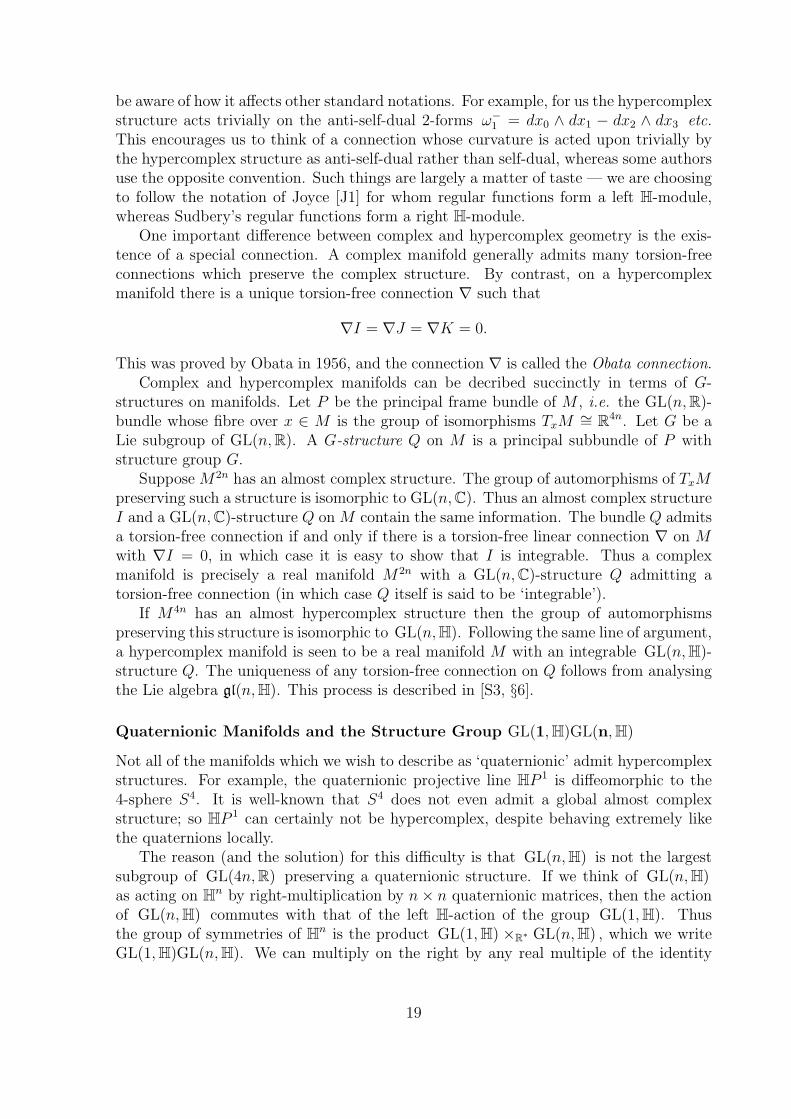
be aware of how it affects other standard notations. For example, for us the hypercomplexstructure acts trivially on the anti-self-dual 2-forms ω−1 = dx0 ∧ dx1 − dx2 ∧ dx3 etc.This encourages us to think of a connection whose curvature is acted upon trivially bythe hypercomplex structure as anti-self-dual rather than self-dual, whereas some authorsuse the opposite convention. Such things are largely a matter of taste — we are choosingto follow the notation of Joyce [J1] for whom regular functions form a left H-module,whereas Sudbery’s regular functions form a right H-module.

One important difference between complex and hypercomplex geometry is the exis-tence of a special connection. A complex manifold generally admits many torsion-freeconnections which preserve the complex structure. By contrast, on a hypercomplexmanifold there is a unique torsion-free connection ∇ such that

∇I = ∇J = ∇K = 0.

This was proved by Obata in 1956, and the connection ∇ is called the Obata connection.Complex and hypercomplex manifolds can be decribed succinctly in terms of G-

structures on manifolds. Let P be the principal frame bundle of M , i.e. the GL(n,R)-bundle whose fibre over x ∈ M is the group of isomorphisms TxM ∼= R4n. Let G be aLie subgroup of GL(n,R). A G-structure Q on M is a principal subbundle of P withstructure group G.

Suppose M2n has an almost complex structure. The group of automorphisms of TxMpreserving such a structure is isomorphic to GL(n,C). Thus an almost complex structureI and a GL(n,C)-structure Q on M contain the same information. The bundle Q admitsa torsion-free connection if and only if there is a torsion-free linear connection ∇ on Mwith ∇I = 0, in which case it is easy to show that I is integrable. Thus a complexmanifold is precisely a real manifold M2n with a GL(n,C)-structure Q admitting atorsion-free connection (in which case Q itself is said to be ‘integrable’).

If M4n has an almost hypercomplex structure then the group of automorphismspreserving this structure is isomorphic to GL(n,H). Following the same line of argument,a hypercomplex manifold is seen to be a real manifold M with an integrable GL(n,H)-structure Q. The uniqueness of any torsion-free connection on Q follows from analysingthe Lie algebra gl(n,H). This process is described in [S3, §6].

Quaternionic Manifolds and the Structure Group GL(1,H)GL(n,H)

Not all of the manifolds which we wish to describe as ‘quaternionic’ admit hypercomplexstructures. For example, the quaternionic projective line HP 1 is diffeomorphic to the4-sphere S4. It is well-known that S4 does not even admit a global almost complexstructure; so HP 1 can certainly not be hypercomplex, despite behaving extremely likethe quaternions locally.

The reason (and the solution) for this difficulty is that GL(n,H) is not the largestsubgroup of GL(4n,R) preserving a quaternionic structure. If we think of GL(n,H)as acting on Hn by right-multiplication by n× n quaternionic matrices, then the actionof GL(n,H) commutes with that of the left H-action of the group GL(1,H). Thusthe group of symmetries of Hn is the product GL(1,H) ×R∗ GL(n,H) , which we writeGL(1,H)GL(n,H). We can multiply on the right by any real multiple of the identity

19

(since GL(1,H) and GL(n,H) share the same centre R∗), so without loss of gener-ality we can reduce the first factor to Sp(1). Thus GL(1,H)GL(n,H) is the same asSp(1)GL(n,H) = Sp(1)×Z2 GL(n,H).

Definition 2.1.2 [S3, 1.1] A quaternionic manifold is a 4n-dimensional real manifold M(n ≥ 2) with an Sp(1)GL(n,H)-structure Q admitting a torsion-free connection.

When n = 1 the situation is different, since Sp(1)×Sp(1) ∼= SO(4). In four dimensionswe make the special definition that a quaternionic manifold is a self-dual conformalmanifold.

In terms of tensors, quaternionic manifolds are a generalisation of hypercomplexmanifolds in the following way. Each tangent space TxM still admits a hypercomplexstructure giving an isomorphism TxM ∼= Hn, but this isomorphism does not necessarilyarise from globally defined complex structures on M . There is still an S2-bundle oflocal almost-complex structures which satisfy IJ = K, but it is free to ‘rotate’. For acomprehensive study of quaternionic manifolds see [S3] and Chapter 9 of [S4].

Riemannian Manifolds in Complex and Quaternionic Geometry

Suppose the GL(n,C)-structure Q on a complex manifold M admits a further reduc-tion to an integrable U(n)-structure Q′. Then M admits a Riemannian metric g withg(IX, IY ) = g(X, Y ) for all X, Y ∈ TxM for all x ∈M . We also define the differentiable2-form ω(X, Y ) = g(IX, Y ). If such a metric arises from an integrable U(n)-structureQ′ then ω will be a closed 2-form, and M is a symplectic manifold — so M has com-patible complex and symplectic structures. In this case M is called a Kahler manifold;an integrable U(n)-structure is called a Kahler structure; the metric g is called a Kahlermetric and the symplectic form ω is called a Kahler form.

The quaternionic analogue of the compact group U(n) is the group Sp(n). A hyper-complex manifold whose GL(n,H)-structure Q reduces to an integrable Sp(n)-structureQ′ admits a metric g which is simultaneously Kahler for each of the complex structuresI, J and K. Such a manifold is called hyperkahler . Using each of the complex structures,we define three independent symplectic forms ωI , ωJ and ωK . Then the complex 2-formωJ + iωK is holomorphic with respect to the complex structure I, and a hyperkahlermanifold has compatible hypercomplex and complex-symplectic structures. Hyperkahlermanifolds are studied in [HKLR], which gives a quotient construction for hyperkahlermanifolds.

Similarly, if a quaternionic manifold has a metric compatible with the torsion-freeSp(1)GL(n,H)-structure, then the Sp(1)GL(n,H)-structure Q reduces to an Sp(1)Sp(n)-structure Q′ and M is said to be quaternionic Kahler. The group Sp(1)Sp(n) is amaximal proper subgroup of SO(4n) except when n = 1, where as we know Sp(1)Sp(1) =SO(4). In four dimensions a manifold is said to be quaternionic Kahler if and only if itis self-dual and Einstein. Quaternionic Kahler manifolds are the subject of [S2].

2.2 Differential Forms on Complex Manifolds

This section consists of background material in complex geometry, especially ideas whichencourage the development of interesting quaternionic versions. More information on this

20

and other aspects of complex geometry can be found in [W] and [GH, §0.2].Let (M, I) be a complex manifold. Then I gives TM and T ∗M the structure of a

U(1)-representation and the complexification C⊗RTM splits into two weight spaces withweights ±i. The same is true of C ⊗R T

∗M . There are various ways of writing theseweight spaces; fairly standard is the notation C⊗R T

∗M = T ∗1,0M ⊕ T ∗0,1M , where thesesummands are the +i and −i eigenspaces of I respectively. However, for our purposesit will be more useful to adopt the notation of [S3], writing

C⊗R T∗M = Λ1,0M ⊕ Λ0,1M, (2.1)

so Λ1,0M = T ∗1,0M and Λ0,1M = T ∗0,1M . A holomorphic function f ∈ C∞(M,C) isa smooth function whose derivative takes values only in Λ1,0M for all m ∈ M , i.e. fis holomorphic if and only if df ∈ C∞(M,Λ1,0M). A closely linked statement is thatΛ1,0M is a holomorphic vector bundle. Thus Λ1,0M is called the holomorphic cotangentspace and Λ0,1M is called the antiholomorphic cotangent space of M . If we reverse thesense of the complex structure (i.e. if we swap I for −I) then we reverse the roles of theholomorphic and antiholomorphic spaces, which is why a function which is holomorphicwith respect to I is antiholomorphic with respect to −I.

From standard multilinear algebra, the decomposition (2.1) gives rise to a decompo-sition of exterior forms of all powers

C⊗R ΛkT ∗M =k⊕

p=0

Λp(T ∗1,0M)⊗ Λk−p(T ∗0,1M).

Define the bundleΛp,qM = ΛpT ∗1,0M ⊗ ΛqT ∗0,1M. (2.2)

With this notation, Equation (2.1) is an example of the more general decomposition intotypes

C⊗R ΛkT ∗M =⊕

p+q=k

Λp,qM. (2.3)

A smooth section of the bundle Λp,qM is called a differential form of type (p, q) or justa (p, q)-form. We write Ωp,q(M) for the set of (p, q)-forms on M , so

Ωp,q(M) = C∞(M,Λp,qM) and Ωk(M) =⊕

p+q=k

Ωp,q(M).

Define two first-order differential operators,

∂ : Ωp,q(M)→ Ωp+1,q(M)∂ = πp+1,q d and

∂ : Ωp,q(M)→ Ωp,q+1(M)

∂ = πp,q+1 d, (2.4)

where πp,q denotes the natural projection from C ⊗ ΛkM onto Λp,qM . The operator ∂is called the Dolbeault operator.

These definitions rely only on the fact that I is an almost complex structure. Acrucial fact is that if I is integrable, these are the only two components represented in

21

Figure 2.1: The Dolbeault Complex

Ω0,0 = C∞(M,C)

*

HHHH

HHj

∂

∂

Ω1,0

*

HHHH

HHj

∂

∂

Ω0,1

*

HHHHHHj

∂

∂

Ω1,1

*

HHHH

HHj

∂

∂

Ω2,0

HHHHH

Hj∂

. . . . . . etc.

Ω0,2

*∂

. . . . . . etc.

the exterior differential d, i.e. d = ∂+ ∂ [WW, Proposition 2.2.2, p.105]. An immediateconsequence of this is that on a complex manifold M ,

∂2 = ∂∂ + ∂∂ = ∂2

= 0. (2.5)

This gives rise to the Dolbeault complex. Writing ∂p,q

for the particular map ∂ :Ωp,q → Ωp,q+1, we define the Dolbeault cohomology groups

Hp,q

∂=

Ker(∂p,q

)

Im(∂p,q−1

).

A function f ∈ C∞(M,C) is holomorphic if and only if ∂f = 0 and for this reason ∂ issometimes called the Cauchy-Riemann operator. Similarly, a (p, 0)-form α is said to beholomorphic if and only if ∂α = 0.

A useful way to think of the Dolbeault complex is as a decomposition of C⊗ΛkT ∗Minto types of U(1)-representation. The representations of U(1) on complex vector spacesare particularly easy to understand. Since U(1) is abelian, the irreducible representationsall are one-dimensional. They are parametrised by the integers, taking the form

%n : U(1)→ GL(1,C) = C∗ %n : eiθ → eniθ

for some n ∈ Z. Representations of the Lie algebra u(1) are then of the form d%n : z →nz. The Dolbeault complex begins with the representation of the complex structure〈I〉 ∼= u(1) on C ⊗ T ∗M . This induces a representation on C ⊗ Λ•T ∗M . It is easyto see that if ω ∈ Λp,qM , I(ω) = i(p − q)ω. In other words, Λp,qM is the bundle ofU(1)-representations of the type %p−q.

22

2.3 Differential Forms on Quaternionic Manifolds

Any G-structure on a manifold M induces a representation of G on the exterior algebraof M . Fujiki’s account of this [F, §2] explains many quaternionic analogues of complexand Kahler geometry.

The decomposition of differential forms on quaternionic Kahler manifolds began byconsidering the fundamental 4-form

Ω = ωI ∧ ωI + ωJ ∧ ωJ + ωK ∧ ωK ,

where ωI , ωJ and ωK are the local Kahler forms associated to local almost complexstructures I, J and K with IJ = K. The fundamental 4-form is globally defined andinvariant under the induced action of Sp(1)Sp(n) on Λ4T ∗M . Kraines [Kr] and Bonan[Bon] used the fundamental 4-form to decompose the space ΛkT ∗M in a similar way tothe Lefschetz decomposition of differential forms on a Kahler manifold [GH, p. 122]. Adifferential k-form µ is said to be effective if Ω∧∗µ = 0, where ∗ : ΛkT ∗M → Λ4n−kT ∗Mis the Hodge star. This leads to the following theorem:

Theorem 2.3.1 [Kr, Theorem 3.5][Bon, Theorem 2]For k ≤ 2n+ 2, every every k-form φ admits a unique decomposition

φ =∑

0≤j≤k/4

Ωj ∧ µk−4j,

where the µk−4j are effective (k − 4j)-forms.

Bonan further refines this decomposition for quaternion-valued forms, using exteriormultiplication by the globally defined quaternionic 2-form Ψ = i1ωI + i2ωJ + i3ωK . Notethat Ψ ∧Ψ = −2Ω.

Another way to consider the decomposition of forms on a quaternionic manifold is asrepresentations of the group Sp(1)GL(n,H). We express the Sp(1)GL(n,H)-representationon Hn by writing

Hn ∼= V1 ⊗ E, (2.6)

where V1 is the basic representation of Sp(1) on C2 and E is the basic representationof GL(n,H) on C2n. (This uses the standard convention of working with complexrepresentations, which in the presence of suitable structure maps can be thought of ascomplexified real representations. In this case, the structure map is the tensor productof the quaternionic structures on V1 and E.)

This representation also describes the (co)tangent bundle of a quaternionic manifoldin the following way. Let P be a principal G-bundle over the differentiable manifold Mand let W be a G-module. We define the associated bundle

W = P ×G W =P ×WG

,

where g ∈ G acts on (p, w) ∈ P ×W by (p, w) · g = (f · g, g−1 ·w). Then W is a vectorbundle over M with fibre W . We will usually just write W for W, relying on context

23

to distinguish between the bundle and the representation. Following Salamon [S3, §1],if M4n is a quaternionic manifold with Sp(1)GL(n,H)-structure Q, then the cotangentbundle is a vector bundle associated to the principal bundle Q and the representationV1 ⊗ E, so that we write

(T ∗M)C ∼= V1 ⊗ E (2.7)

(though we will usually omit the complexification sign). This induces an Sp(1)GL(n,H)-action on the bundle of exterior k-forms ΛkT ∗M ,

ΛkT ∗M ∼= Λk(V1 ⊗ E) ∼=[k/2]⊕j=0

Sk−2j(V1)⊗ Lkj∼=

[k/2]⊕j=0

Vk−2j ⊗ Lkj , (2.8)

where Lkj is an irreducible representation of GL(n,H). This decomposition is given

by Salamon [S3, §4], along with more details concerning the nature of the GL(n,H)representations Lk

j . If M is quaternion Kahler, ΛkT ∗M can be further decomposedinto representations of the compact group Sp(1)Sp(n). This refinement is performed indetail by Swann [Sw], and used to demonstrate significant results.

If we symmetrise completely on V1 in Equation (2.8) to obtain Vk, we must antisym-metrise completely on E. Salamon therefore defines the irreducible subspace

Ak ∼= Vk ⊗ ΛkE. (2.9)

The bundle Ak can be described using the decomposition into types for the local almostcomplex structures on M as follows [S3, Proposition 4.2]: 2

Ak =∑I∈S2

Λk,0I M. (2.10)

Letting p denote the natural projection p : ΛkT ∗M → Ak and setting D = p d, wedefine a sequence of differential operators

0 −→ C∞(A0)D=d−→ C∞(A1 = T ∗M)

D−→ C∞(A2)D−→ . . .

D−→ C∞(A2n) −→ 0. (2.11)

This is accomplished using only the fact that M has an Sp(1)GL(n,H)-structure; sucha manifold is called ‘almost quaternionic’. The following theorem of Salamon relates theintegrability of such a structure with the sequence of operators in (2.11):

Theorem 2.3.2 [S3, Theorem 4.1] An almost quaternionic manifold is quaternionic ifand only if (2.11) is a complex.

This theorem is analogous to the familiar result in complex geometry that an almost

complex structure on a manifold is integrable if and only if ∂2

= 0.

2This is because every Sp(1)-representation Vn is generated by its highest weight spaces taken withrespect to all the different linear combinations of I, J and K. We will use such descriptions in detail inlater chapters, and find that they play a prominent role in quaternionic algebra.

24

Chapter 3

A Double Complex on QuaternionicManifolds

Until now we have been discussing known material. In this chapter we present a discoverywhich as far as the author can tell is new — a double complex of exterior forms onquaternionic manifolds. We argue that this is the best quaternionic analogue of theDolbeault complex. The ‘top row’ of this double complex is exactly the complex (2.11)discovered by Simon Salamon, which plays a similar role to that of the (k, 0)-forms on acomplex manifold.

The new double complex is obtained by simplifying the Bonan decomposition ofEquation (2.8). Instead of using the more complicated structure of ΛkT ∗M as anSp(1)GL(n,H)-module, we consider only the action of the Sp(1)-factor and decomposeΛkT ∗M into irreducible Sp(1)-representations — a fairly easy process achieved by con-sidering weights. The resulting decomposition gives rise to a double complex throughthe Clebsch-Gordon formula, in particular the isomorphism Vr⊗V1

∼= Vr+1⊕Vr−1. Thisencourages us to define two ‘quaternionic Dolbeault’ operators D and D, and leads tonew cohomology groups on quaternionic manifolds.

The main geometric difference between this double complex and the Dolbeault com-plex is that whilst the Dolbeault complex is a diamond, our double complex forms anisosceles triangle, as if the diamond is ‘folded in half’. This is more like the decompositionof real-valued forms on complex manifolds.

Determining where our double complex is elliptic has been far more difficult than forthe de Rham or Dolbeault complexes. The ellipticity properties of our double complex aremore similar to those of a real-valued version of the Dolbeault complex. Because of thissimilarity, we shall begin with a discussion of real-valued forms on complex manifolds.

3.1 Real forms on Complex Manifolds

Let M be a complex manifold and let ω ∈ Λp,q = Λp,qM . Then ω ∈ Λq,p, and so ω + ωis a real-valued exterior form in (Λp,q ⊕ Λq,p)R, where the subscript R denotes the factthat we are talking about real forms. The space (Λp,q ⊕ Λq,p)R is a real vector bundleassociated to the principal GL(n,C)-bundle defined by the complex structure. This gives

25

a decomposition of real-valued exterior forms, 1

ΛkRT

∗M =⊕

p+q=kp>q

(Λp,q ⊕ Λq,p)R ⊕ Λk2, k2

R . (3.1)

The condition p > q ensures that we have no repetition. The bundle Λk2, k2

R only appearswhen k is even. It is its own conjugate and so naturally a real vector bundle associatedto the trivial representation of U(1).

Let ω + ω ∈ (Ωp,q ⊕ Ωq,p)R. Then ∂ω + ∂ω ∈ (Ωp+1,q ⊕ Ωq,p+1)R. Call this operator∂ ⊕ ∂. Then

d(ω + ω) = (∂ ⊕ ∂)(ω + ω) + (∂ ⊕ ∂)(ω + ω)

∈ (Ωp+1,q ⊕ Ωq,p+1)R ⊕ (Ωp,q+1 ⊕ Ωq+1,p)R.

When p = q, ω = ω, so ∂ ⊕ ∂ = ∂ ⊕ ∂ = d, and there is only one differential operatoracting on Ωp,p. This gives the following double complex (where the real subscripts areomitted for convenience).

Figure 3.1: The Real Dolbeault Complex

Ω0,0 = C∞(M)

*

d

Ω1,0 ⊕ Ω0,1

*

HHHHH

Hj

∂ ⊕ ∂

∂ ⊕ ∂Ω1,1

*d

Ω2,0 ⊕ Ω0,2

*

HHHHH

Hj

∂ ⊕ ∂

∂ ⊕ ∂Ω2,1 ⊕ Ω1,2

*

HHHHH

Hj

∂ ⊕ ∂

∂ ⊕ ∂

. . . . . . etc.

Ω3,0 ⊕ Ω0,3

HHHHHHj∂ ⊕ ∂

. . . . . . etc.

Thus there is a double complex of real forms on a complex manifold, obtained bydecomposing Λk

xT∗M into subrepresentations of the action of u(1) = 〈I〉, induced from

the action on T ∗xM . This double complex is less well-behaved than its complex-valuedcounterpart; in particular, it is not elliptic everywhere. We shall now show what thismeans, and why it is significant.

Ellipticity

Whether or not a differential complex on a manifold is ‘elliptic’ is an important ques-tion, with striking topological, algebraic and physical consequences. Examples of elliptic

1This decomposition is also given by Reyes-Carion [R, §3.1], who calls the bundle (Λp,q ⊕ Λq,p)R[[Λp,q]].

26

complexes include the de Rham and Dolbeault complexes. A thorough description ofelliptic operators and elliptic complexes can be found in [W, Chapter 5].

Let E and F be vector bundles over M , and let Φ : C∞(E)→ C∞(F ) be a differentialoperator. (We will be working with first-order operators, and so will only describe thiscase.) At every point x ∈ M and for every nonzero ξ ∈ T ∗xM , we define a linear mapσΦ(x, ξ) : Ex → Fx called the principal symbol of Φ, as follows. Let ε ∈ C∞(E) withε(x) = e, and let f ∈ C∞(M) with f(x) = 0, df(x) = ξ. Then

σΦ(x, ξ)e = Φ(fε)|x.

In coordinates, σ is often found by replacing the operator ∂∂xj with exterior multiplication

by a cotangent vector ξj dual to ∂∂xj . For example, for the exterior differential d :

Ωk(M)→ Ωk+1(M) we have σd(x, ξ)ω = ω ∧ ξ. The operator Φ is said to be elliptic atx ∈M if the symbol σΦ(x, ξ) : Ex → Fx is an isomorphism for all nonzero ξ ∈ T ∗xM .

A complex 0Φ0−→ C∞(E0)

Φ1−→ C∞(E1)Φ2−→ C∞(E2)

Φ3−→ . . .Φn−→ C∞(En)

Φn+1−→ 0 is

said to be elliptic at Ei if the symbol sequence Ei−1

σΦi−→ Ei

σΦi+1−→ Ei+1 is exact for allξ ∈ T ∗xM and for all x ∈M . The link between these two forms of ellipticity is as follows.If we have a metric on each Ei then we can define a formal adjoint Φ∗

i : Ei → Ei−1.Linear algebra reveals that the complex is elliptic at Ei if and only if the LaplacianΦ∗

i Φi + Φi−1Φ∗i−1 is an elliptic operator.

One important implication of this is that an elliptic complex on a compact manifoldhas finite-dimensional cohomology groups [W, Theorem 5.2, p. 147]. Whether a complexyields interesting cohomological information is in this way directly related to whether ornot the complex is elliptic. The following Proposition answers this question for the realDolbeault complex.

Proposition 3.1.1 For p > 0, the upward complex

0 −→ Ωp,p −→ Ωp+1,p ⊕ Ωp,p+1 −→ Ωp+2,p ⊕ Ωp,p+2 −→ . . .

is elliptic everywhere except at the first two spaces Ωp,p and Ωp+1,p ⊕ Ωp,p+1.For p = 0, the ‘leading edge’ complex

0 −→ Ω0,0 −→ Ω1,0 ⊕ Ω0,1 −→ Ω2,0 ⊕ Ω0,2 −→ . . .

is elliptic everywhere except at Ω1,0 ⊕ Ω0,1 = Ω1(M).

Proof. When p > q + 1, we have short sequences of the form

Ωp−1,q ∂−→ Ωp,q ∂−→ Ωp+1,q⊕ ⊕ ⊕Ωq,p−1 ∂−→ Ωq,p ∂−→ Ωq,p+1.

(3.2)

Each such sequence is (a real subspace of) the direct sum of two elliptic sequences, andso is elliptic. Thus we have ellipticity at Ωp,q ⊕ Ωq,p whenever p ≥ q + 2.

27

This leaves us to consider the case when p = q, and the sequence

0 −→ Ωp,p

∂

∂

Ωp+1,p ∂−→ Ωp+2,2 −→ . . . etc.⊕ ⊕Ωp,p+1 ∂−→ Ω2,p+2 −→ . . . etc.

(3.3)

This fails to be elliptic. An easy and instructive way to see this is to consider the simplest4-dimensional example M = C2.

Let e0, e1 = I(e0), e2 and e3 = I(e2) form a basis for T ∗x C2 ∼= C2, and let eab...

denote ea ∧ eb ∧ . . . etc. Then I(e01) = e00 − e11 = 0, so e01 ∈ Λ1,1. The map from Λ1,1

to Λ2,1 ⊕ Λ1,2 is just the exterior differential d. Since σd(x, e0)(e01) = e01 ∧ e0 = 0 the

symbol map σd : Λ1,1 → Λ2,1⊕Λ1,2 is not injective, so the symbol sequence is not exactat Λ1,1.

Consider also e123 ∈ Λ2,1⊕Λ1,2. Then σ∂⊕∂(x, e0)(e123) = 0, since there is no bundle

Λ3,1 ⊕ Λ1,3. But e123 has no e0-factor, so is not the image under σd(x, e0) of any form

α ∈ Λ1,1. Thus the symbol sequence fails to be exact at Λ2,1 ⊕ Λ1,2.It is a simple matter to extend these counterexamples to higher dimensions and higher

exterior powers. For k = 0, the situation is different. It is easy to show that the complex

0 −→ C∞(M)d−→ Ω1,0 ⊕ Ω0,1 ∂⊕∂−→ Ω2,0 ⊕ Ω0,2 −→ . . . etc.

is elliptic everywhere except at (Ω1,0 ⊕ Ω0,1).

This last sequence is given particular attention by Reyes-Carion [R, Lemma 2]. Heshows that, when M is Kahler, ellipticity can be regained by adding the space 〈ω〉 tothe bundle Λ2,0 ⊕ Λ0,2, where ω is the real Kahler (1, 1)-form.

The Real Dolbeault complex is thus elliptic except at the bottom of the isoscelestriangle of spaces. Here the projection from d(Ωp,p) to Ωp+1,p ⊕ Ωp,p+1 is the identity,and arguments based upon non-trivial projection maps no longer apply. We shall seethat this situation is closely akin to that of differential forms on quaternionic manifolds,and that techniques motivated by this example yield similar results.

3.2 Construction of the Double Complex

Let M4n be a quaternionic manifold. Then T ∗xM∼= V1 ⊗ E as an Sp(1)GL(n,H)-

representation for all x ∈ M . Suppose we consider just the action of the Sp(1)-factor.Then the (complexified) cotangent space effectively takes the form V1 ⊗ C2n ∼= 2nV1.Thus the Sp(1)-action on ΛkT ∗M is given by the representation Λk(2nV1).

To work out the irreducible decomposition of this representation we compute theweight space decomposition of Λk(2nV1) from that of 2nV1.

2 With respect to theaction of a particular subgroup U(1)q ⊂ Sp(1), the representation 2nV1 has weights+1 and −1, each occuring with multiplicity 2n. The weights of Λk(2nV1) are the k-wise distinct sums of these. Each weight r in Λk(2nV1) must therefore be a sum of poccurences of the weight ‘+1’ and p− r occurences of the weight ‘−1’, where 2p− r = k

2This process for calculating the weights of tensor, symmetric and exterior powers is a standardtechnique in representation theory — see for example [FH, §11.2].

28

and 0 ≤ p ≤ k (from which it follows immediately that −k ≤ r ≤ k and r ≡ k mod 2).The number of ways to choose the p ‘+1’ weights is

(2np

), and the number of ways

to choose the (p − r) ‘−1’ weights is(

2np−r

), so the multiplicity of the weight r in the

representation Λk(2nV1) is

Mult(r) =

(2nk+r2

)(2nk−r2

).

For r ≥ 0, consider the difference Mult(r)−Mult(r+2). This is the number of weightspaces of weight r which do not have any corresponding weight space of weight r + 2.Each such weight space must therefore be the highest weight space in an irreduciblesubrepresentation Vr ⊆ ΛkT ∗M , from which it follows that the number of irreduciblesVr in Λk(2nV1) is equal to Mult(r)−Mult(r + 2). This demonstrates the followingProposition:

Proposition 3.2.1 Let M4n be a hypercomplex manifold. The decomposition into irre-ducibles of the induced representation of Sp(1) on ΛkT ∗M is

ΛkT ∗M ∼=k⊕

r=0

[(2nk+r2

)(2nk−r2

)−(

2nk+r+2

2

)(2n

k−r−22

)]Vr,

where r ≡ k mod 2.

We will not always write the condition r ≡ k mod 2, assuming that(

pq

)= 0 if q 6∈ Z.

Definition 3.2.2 Let M4n be a quaternionic manifold. Define the coefficient

εnk,r =

(2nk+r2

)(2nk−r2

)−(

2nk+r+2

2

)(2n

k−r−22

),

and let Ek,r be the vector bundle associated to the Sp(1)-representation εnk,rVr. Withthis notation Proposition 3.2.1 is written

ΛkT ∗M ∼=k⊕

r=0

εnk,rVr =k⊕

r=0

Ek,r.

Our most important result is that this decomposition gives rise to a double complexof differential forms and operators on a quaternionic manifold.

Theorem 3.2.3 The exterior derivative d maps C∞(M,Ek,r) to C∞(M,Ek+1,r+1 ⊕Ek+1,r−1).

Proof. Let ∇ be a torsion-free linear connection on M preserving the quaternionicstructure. Then ∇ : C∞(M,Ek,r) → C∞(M,Ek,r ⊗ T ∗M). As Sp(1)-representations,this is

∇ : C∞(M, εnk,rVr)→ C∞(M, εnk,rVr ⊗ 2nV1).

29

Using the Clebsch-Gordon formula we have εnk,rVr⊗2nV1∼= 2nεnk,r(Vr+1⊕Vr−1). Thus the

image of Ek,r under ∇ is contained in the Vr+1 and Vr−1 summands of ΛkT ∗M ⊗ T ∗M .Since ∇ is torsion-free, d = ∧ ∇, so d maps (sections of) Ek,r to the Vr+1 and Vr−1

summands of Λk+1T ∗M . Thus d : C∞(M,Ek,r)→ C∞(M,Ek+1,r+1 ⊕ Ek+1,r−1).

This allows us to split the exterior differential d into two ‘quaternionic Dolbeaultoperators’.

Definition 3.2.4 Let πk,r be the natural projection from ΛkT ∗M onto Ek,r. Define theoperators

D : C∞(Ek,r)→ C∞(Ek+1,r+1)D = πk+1,r+1 d

andD : C∞(Ek,r)→ C∞(Ek+1,r−1)D = πk+1,r−1 d.

(3.4)

Theorem 3.2.3 is equivalent to the following:

Proposition 3.2.5 On a quaternionic manifold M , we have d = D +D, and so

D2 = DD +DD = D2= 0.

Proof. The first equation is equivalent to Theorem 3.2.3. The rest follows immediatelyfrom decomposing the equation d2 = 0.

Figure 3.2: The Double Complex

C∞(E0,0 = R)

*DC∞(E1,1 = T ∗M)

*

HHHHHHj

D

DC∞(E2,0)

*D

C∞(E2,2)

*

HHHH

HHj

D

DC∞(E3,1)

*

HHHHHHj

D

D

. . . . . . etc.

C∞(E3,3)H

HHHHHjD

. . . . . . etc.

Here is our quaternionic analogue of the Dolbeault complex. There are strong sim-ilarities between this and the Real Dolbeault complex (Figure 3.1). Again, instead ofa diamond as in the Dolbeault complex, the quaternionic version only extends upwardsto form an isosceles triangle. This is essentially because there is one irreducible U(1)-representation for each integer, whereas there is one irreducible Sp(1)-representation onlyfor each nonnegative integer. Note that this is a decomposition of real as well as complexdifferential forms; the operators D and D map real forms to real forms.

30

By definition, the bundle Ek,k is the bundle Ak of (2.9) — they are both the subbundleof ΛkT ∗M which includes all Sp(1)-representations of the form Vk. Thus the leading edgeof the double complex

0 −→ C∞(E0,0)D−→ C∞(E1,1)

D−→ C∞(E2,2)D−→ . . .

D−→ C∞(E2n,2n)D−→ 0

is precisely the complex (2.11) discovered by Salamon.

Example 3.2.6 Four DimensionsThis double complex is already very well-known and understood in four dimensions.

Here there is a splitting only in the middle dimension, Λ2T ∗M ∼= V2 ⊕ 3V0. Let I, Jand K be local almost complex structures at x ∈M , and let e0 ∈ T ∗xM . Let e1 = I(e0),e2 = J(e0) and e3 = K(e0). In this way we obtain a basis e0, . . . , e3 for T ∗xM

∼= H.Using the notation eijk... = ei ∧ ej ∧ ek ∧ . . .etc., define the 2-forms

ω±1 = e01 ± e23, ω±2 = e02 ± e31, ω±3 = e03 ± e12. (3.5)

Then I, J and K all act trivially 3 on the ω−j , so E2,0 = 〈ω−1 , ω−2 , ω−3 〉. The action ofsp(1) on the ω+

j is given by the multiplication table

I(ω+1 ) = 0

J(ω+1 ) = −2ω+

3

K(ω+1 ) = 2ω+

2

I(ω+2 ) = 2ω+

3

J(ω+2 ) = 0

K(ω+2 ) = −2ω+

1

I(ω+3 ) = −2ω+

3

J(ω+3 ) = 2ω+

1

K(ω+3 ) = 0.

(3.6)

These are the relations of the irreducible sp(1)-representation V2, and we see that E2,2 =〈ω+

1 , ω+2 , ω

+3 〉.

These bundles will be familiar to most readers: E2,2 is the bundle of self-dual 2-forms Λ2

+ and E2,0 is the bundle of anti-self-dual 2-forms Λ2−. The celebrated splitting

Λ2T ∗M ∼= Λ2+⊕Λ2

− is an invariant of the conformal class of any Riemannian 4-manifold,and I2 + J2 +K2 = −4(∗+ 1), where ∗ : ΛkT ∗M → Λ4−kT ∗M is the Hodge star map.

This also serves to illustrate why in four dimensions we make the definition thata quaternionic manifold is a self-dual conformal manifold. The relationship betweenquaternionic, almost complex and Riemannian structures in four dimensions is describedin more detail in [S4, Chapter 7], a classic reference being [AHS].

Because there is no suitable quaternionic version of holomorphic coordinates, there isno ‘nice’ co-ordinate expression for a typical section of C∞(Ek,r). In order to determinethe decomposition of a differential form, the simplest way the author has found is to usethe Casimir operator C = I2 + J2 + K2. Consider a k-form α. Then α ∈ Ek,r if andonly if (I2 + J2 + K2)(α) = −r(r + 2)α. This mechanism also allows us to work outexpressions for D and D acting on α.

Lemma 3.2.7 Let α ∈ C∞(Ek,r). Then

Dα = −1

4

((r − 1) +

1

r + 1(I2 + J2 +K2)

)dα

3We are assuming throughout that uppercase operators like I, J and K are acting as elements of aLie algebra, not a Lie group. This makes no difference on T ∗M but is important on the exterior powersΛkT ∗M . In particular, for k 6= 1 we no longer expect I2 = J2 = K2 = −1, and by ‘act trivially’ wemean ‘annihilate’.

31

and

Dα =1

4

((r + 3) +

1

r + 1(I2 + J2 +K2)

)dα.

Proof. We have dα = Dα+Dα, where Dα ∈ Ek+1,r+1 and Dα ∈ Ek+1,r−1. Applying theCasimir operator gives

(I2 + J2 +K2)(dα) = −(r + 1)(r + 3)Dα− (r + 1)(r − 1)Dα.

Rearranging these equations gives Dα and Dα.

Writing Dk,r for the particular map D : C∞(Ek,r) → C∞(Ek+1,r+1), we define thequaternionic cohomology groups

Hk,rD (M) =

Ker(Dk,r)

Im(Dk−1,r−1). (3.7)

3.3 Ellipticity and the Double Complex

In this section we shall determine where our double complex is elliptic and where it isnot. It turns out that we have ellipticity everywhere except on the bottom two rows ofthe complex. This is exactly like the real Dolbeault complex of Figure 3.1, and thoughit is more difficult to prove for the quaternionic version, the guiding principles whichdetermine where the two double complexes are elliptic are very much the same in bothcases.

Here is the main result of this section:

Theorem 3.3.1 For 2k ≥ 4, the complex

0→ E2k,0D→ E2k+1,1

D→ E2k+2,2D→ . . .

D→ E2n+k,2n−kD→ 0

is elliptic everywhere except at E2k,0 and E2k+1,1, where it is not elliptic.For k = 1 the complex is elliptic everywhere except at E3,1, where it is not elliptic.For k = 0 the complex is elliptic everywhere.

The rest of this section provides a proof of this Theorem. Note the strong similaritybetween this Theorem and Proposition 3.1.1, the analogous result for the Real Dolbeaultcomplex. Again, it is the isosceles triangle as opposed to diamond shape which causesellipticity to fail for the bottom row, because d = D on E2k,0 and the projection fromd(C∞(E2k,0)) to C∞(E2k+1,1) is the identity.

On a complex manifold M2n with holomorphic coordinates zj, the exterior formsdza1 ∧ . . . ∧ dzap ∧ dzb1 ∧ . . . ∧ dzbq span Λp,q. This allows us to decompose any formω ∈ Λp,q, making it much easier to write down the kernels and images of maps whichinvolve exterior multiplication. On a quaternionic manifoldM4n there is unfortunately noeasy way to write down a local frame for the bundle Ek,r, because there is no quaternionicversion of ‘holomorphic coordinates’. However, we can decompose Ek,r just enough toenable us to prove Theorem 3.3.1.

32

A principal observation is that since ellipticity is a local property, we can work on Hn

without loss of generality. Secondly, since GL(n,H) acts transitively on Hn \ 0, if the

symbol sequence . . .σe0−→ Ek,r

σe0−→ Ek+1,r+1

σe0−→ . . . is exact for any nonzero e0 ∈ T ∗Hn

then it is exact for all nonzero ξ ∈ T ∗Hn. To prove Theorem 3.3.1, we choose one suche0 and analyse the spaces Ek,r accordingly.

3.3.1 Decomposition of the Spaces Ek,r

Let e0 ∈ T ∗x Hn ∼= Hn and let (I, J,K) be the standard hypercomplex structure on Hn. Asin Example 3.2.6, define e1 = I(e0), e2 = J(e0) and e3 = K(e0), so that 〈e0, . . . , e3〉 ∼= H.In this way we single out a particular copy of H which we call H0, obtaining a (nonnatural)splitting T ∗x Hn ∼= Hn−1⊕H0 which is preserved by action of the hypercomplex structure.This induces the decomposition ΛkHn ∼=

⊕4l=0 Λk−lHn−1⊗ΛlH0, which decomposes each

Ek,r ⊂ ΛkHn according to how many differentials in the H0-direction are present.

Definition 3.3.2 Define the space Elk,r to be the subspace of Ek,r consisting of exterior

forms with precisely l differentials in the H0-direction, i.e.

Elk,r ≡ Ek,r ∩ (Λk−lHn−1 ⊗ ΛlH0).

Then Elk,r is preserved by the induced action of the hypercomplex structure on ΛkHn.

Thus we obtain an invariant decomposition Ek,r = E0k,r ⊕E1

k,r ⊕E2k,r ⊕E3

k,r ⊕E4k,r. Note

that we can identify E0k,r on Hn with Ek,r on Hn−1.

(Throughout the rest of this section, juxtaposition of exterior forms will denote ex-terior multiplication, for example αeij means α ∧ eij.)

We can decompose these summands still further. Consider, for example, the bun-dle E1

k,r. An exterior form α ∈ E1k,r is of the form α0e

0 + α1e1 + α2e

2 + α3e3, where

αj ∈ Λk−1Hn−1. Thus α is an element of Λk−1Hn−1 ⊗ 2V1, since H0∼= 2V1 as an sp(1)-

representation. Since α is in a copy of the representation Vr, it follows from the isomor-phism Vr ⊗ V1

∼= Vr+1 ⊕ Vr−1 that the αj must be in a combination of Vr+1 and Vr−1

representations, i.e. αj ∈ E0k−1,r+1 ⊕ E0

k−1,r−1. We write

α = α+ + α− = (α+0 + α−0 )e0 + (α+

1 + α−1 )e1 + (α+2 + α−2 )e2 + (α+

3 + α−3 )e3,

where α+j ∈ E0

k−1,r+1 and α−j ∈ E0k−1,r−1.

The following Lemma allows us to consider α+ and α− separately.

Lemma 3.3.3 If α = α+ + α− ∈ E1k,r then both α+ and α− must be in E1

k,r.

Proof. In terms of representations, the situation is of the form

(pVr+1 ⊕ qVr−1)⊗ 2V1∼= 2p(Vr+2 ⊕ Vr)⊕ 2q(Vr ⊕ Vr−2),

where α+ ∈ pVr+1 and α− ∈ qVr−1. For α to be in the representation 2(p + q)Vr,its components in the representations 2pVr+2 and 2qVr−2 must both vanish separately.The component in 2pVr+2 comes entirely from α+, so for this to vanish we must have

33

α+ ∈ 2(p+ q)Vr independently of α−. Similarly, for the component in 2qVr−2 to vanish,we must have α− ∈ 2(p+ q)Vr.

Thus we decompose the space E1k,r into two summands, one coming from E0

k−1,r−1 ⊗2V1 and one from E0

k−1,r+1⊗2V1. We extend this decomposition to the cases l = 0, 2, 3, 4,defining the following notation.

Definition 3.3.4 Define the bundle El,mk,r to be the subbundle of El

k,r arising from

Vm-type representations in Λk−lHn−1. In other words,

El,mk,r ≡ (E0

k−l,m ⊗ ΛlH0) ∩ Ek,r.

To recapitulate: for the space El,mk,r , the bottom left index k refers to the exterior

power of the form α ∈ ΛkHn; the bottom right index r refers to the irreducible Sp(1)-representation in which α lies; the top left index l refers to the number of differentials inthe H0-direction and the top right index m refers to the irreducible Sp(1)-representationof the contributions from Λk−aHn−1 before wedging with forms in the H0-direction. Thismay appear slightly fiddly: it becomes rather simpler when we consider the specificsplittings which Definition 3.3.4 allows us to write down.

Lemma 3.3.5 Let El,mk,r be as above. We have the following decompositions:

E0k,r = E0,r

k,r E1k,r = E1,r+1

k,r ⊕ E1,r−1k,r E2

k,r = E2,r+2k,r ⊕ E2,r

k,r ⊕ E2,r−2k,r

E3k,r = E3,r+1

k,r ⊕ E3,r−1k,r and E4

k,r = E4,rk,r .

Proof. The first isomorphism is trivial, as is the last (since the hypercomplex structureacts trivially on Λ4H0). The second isomorphism is Lemma 3.3.3, and the fourth followsin exactly the same way since Λ3H0

∼= 2V1 also. The middle isomorphism follows asimilar argument.

Recall the self-dual forms and anti-self-dual forms in Example 3.2.6. The bundle E2,rk,r

splits according to whether its contribution from Λ2H0 is self-dual or anti-self-dual. Wewill call these summands E2,r+

k,r and E2,r−k,r respectively, so E2,r

k,r = E2,r+k,r ⊕ E

2,r−k,r .

3.3.2 Lie in conditions

We have analysed the bundle Ek,r into a number of different subbundles. We nowdetermine when a particular exterior form lies in one of these subbundles. Considera form α = α1e

s1...sa + α2et1...ta + . . . etc. where αj ∈ E0

k−a,b. For α to lie in one of the

spaces Ea,bk,r the αj will usually have to satisfy some simultaneous equations. Since these

are the conditions for a form to lie in a particular Lie algebra representation, we willrefer to such equations as ‘Lie in conditions’.

To begin with, we mention three trivial Lie in conditions. Let α ∈ E0k,r. That α ∈ E0,r

k,r

is obvious, as is αe0123 ∈ E4,rk,r , since wedging with e0123 has no effect on the sp(1)-action.

34

Likewise, the sp(1)-action on the anti-self-dual 2-forms ω−1 = e01 − e23, ω−2 = e02 − e31and ω−3 = e03 − e12 is trivial, so αω−j ∈ E

2,r−k,r for all j = 1, 2, 3.

This leaves the following three situations: those arising from taking exterior productswith 1-forms, 3-forms and the self-dual 2-forms ω+

j . As usual when we want to knowwhich representation an exterior form is in, we apply the Casimir operator.

The cases l = 1 and l = 3

Let αj ∈ E0k,r. Then α = α0e

0 + α1e1 + α2e

2 + α3e3 ∈ E1,r

k+1,r+1 ⊕ E1,rk+1,r−1, and α is

entirely in E1,rk+1,r+1 if and only if (I2 + J2 +K2)α = −(r + 1)(r + 3)α.

By the usual (Leibniz) rule for a Lie algebra action on a tensor product, we have thatI2(αje

j) = I2(αj)ej + 2I(αj)I(e

j) + αjI2(ej), etc. Thus

(I2 + J2 +K2)α =3∑

j=0

[(I2 + J2 +K2)(αj)e

j + αj(I2 + J2 +K2)(ej) +

+ 2(I(αj)I(e

j) + J(αj)J(ej) +K(αj)K(ej))]

= −r(r + 2)α− 3α+ 23∑

j=0

(I(αj)I(e

j) + J(αj)J(ej) +K(αj)K(ej))

= (−r2 − 2r − 3)α+ 2(I(α0)e

1 − I(α1)e0 + I(α2)e

3 − I(α3)e2+

+J(α0)e2 − J(α1)e

3 − J(α2)e0 + J(α3)e

1+

+K(α0)e3 +K(α1)e

2 −K(α2)e1 −K(α3)e

0).

(3.8)

For α ∈ E1,rk+1,r+1 we need this to be equal to −(r + 1)(r + 3)α, which is the case if and

only if

−rα = I(α0)e1 − I(α1)e

0 + I(α2)e3 − I(α3)e

2 + J(α0)e2 − J(α1)e

3 − J(α2)e0 + J(α3)e

1 +

+ K(α0)e3 +K(α1)e

2 −K(α2)e1 −K(α3)e

0.

Since the αj have no ej-factors and the action of I, J and K preserves this property,this equation can only be satisfied if it holds for each of the ej-components separately.We conclude that α ∈ E1,r

k+1,r+1 if and only if α0, α1, α2 and α3 satisfy the following Liein conditions: 4

rα0 − I(α1)− J(α2)−K(α3) = 0rα1 + I(α0) + J(α3)−K(α2) = 0rα2 − I(α3) + J(α0) +K(α1) = 0rα3 + I(α2)− J(α1) +K(α0) = 0.

(3.9)

Suppose instead that α ∈ E1,rk+1,r−1. Then (I2+J2+K2)α = −(r−1)(r+1)α. Putting

this alternative into Equation (3.8) gives the result that α ∈ E1,rk+1,r−1 if and only if

4Our interest in these conditions arises from a consideration of exterior forms, but the equationsdescribe sp(1)-representations in general: they are the conditions that α ∈ Vr ⊗V1 must satisfy to be inthe Vr+1 subspace of Vr+1 ⊕ Vr−1

∼= Vr ⊗ V1. The other Lie in conditions have similar interpretations.

35

(r + 2)α0 + I(α1) + J(α2) +K(α3) = 0(r + 2)α1 − I(α0)− J(α3) +K(α2) = 0(r + 2)α2 + I(α3)− J(α0)−K(α1) = 0(r + 2)α3 − I(α2) + J(α1)−K(α0) = 0.

(3.10)

Consider now α = α0e123 + α1e

032 + α2e013 + α3e

021 ∈ E3,rk+3,r+1 ⊕ E3,r

k+3,r−1. Since

Λ3H0∼= H0, the Lie in conditions are exactly the same: for α to be in E3,r

k+3,r+1 we need

the αj to satisfy Equations (3.9), and for α to be in E3,rk+3,r−1 we need the αj to satisfy

Equations (3.10).

The case l = 2

We have already noted that wedging a form β ∈ E0k,r with an anti-self-dual 2-form ω−j

has no effect on the sp(1)-action, so βω−j ∈ E2,r−k+2,r. Thus we only have to consider the

effect of wedging with the self-dual 2-forms 〈ω+1 , ω

+2 , ω

+3 〉 ∼= V2 ⊂ Λ2H0. By the Clebsch-

Gordon formula, the decomposition takes the form Vr ⊗ V2∼= Vr+2 ⊕ Vr ⊕ Vr−2. Thus

for β = β1ω+1 + β2ω

+2 + β3ω

+3 we want to establish the Lie in conditions for β to be in

E2,rk+2,r+2, E

2,r+k+2,r and E2,r

k+2,r−2.We calculate these Lie in conditions in a similar fashion to the previous cases, by con-

sidering the action of the Casimir operator I2+J2+K2 on β and using the multiplicationtable (3.6). The following Lie in conditions are then easy to deduce:

β ∈ E2,rk+2,r+2 ⇐⇒

(r + 4)β1 = J(β3)−K(β2)(r + 4)β2 = K(β1)− I(β3)(r + 4)β3 = I(β2)− J(β1).

(3.11)

β ∈ E2,r+k+2,r ⇐⇒

2β1 = J(β3)−K(β2)2β2 = K(β1)− I(β3)2β3 = I(β2)− J(β1).

(3.12)

β ∈ E2,rk+2,r−2 ⇐⇒

(2− r)β1 = J(β3)−K(β2)(2− r)β2 = K(β1)− I(β3)(2− r)β3 = I(β2)− J(β1).

(3.13)

Equation 3.12 is particularly interesting. Since this equation singles out theVr-representation in the direct sum Vr+2 ⊕ Vr ⊕ Vr+2, it must have dimVr = r + 1linearly independent solutions. Let β0 ∈ Vr and let β1 = I(β0), β2 = J(β0), β3 = K(β0).Using the Lie algebra relations 2I = [J,K] = JK − KJ , it is easy to see that β1, β2

and β3 satisfy Equation 3.12. Moreover, there are r + 1 linearly independent solutionsof this form (for r 6= 0). We conclude that all the solutions of Equation (3.12) take theform β1 = I(β0), β2 = J(β0), β3 = K(β0).

3.3.3 The Symbol Sequence and Proof of Theorem 3.3.1

We now describe the principal symbol of D, and examine its behaviour in the contextof the decompositions of Definition 3.3.2 and Lemma 3.3.5. This leads to a proof ofTheorem 3.3.1. First we obtain the principal symbol from the formula for D in Lemma3.2.7 by replacing dα with αe0.

36

Proposition 3.3.6 Let x ∈ Hn, e0 ∈ T ∗x Hn and α ∈ Ek,r. The principal symbolmapping σD(x, e0) : Ek,r → Ek+1,r+1 is given by

σD(x, e0)(α) =1

2(r + 1)

((r + 2)αe0 − I(α)e1 − J(α)e2 −K(α)e3

).

Proof. Replacing dα with αe0 in the formula for D obtained in Lemma 3.2.7, we have

σD(x, e0)(α) = −1

4

((r − 1) +

1

r + 1(I2 + J2 +K2)

)αe0

=−1

4(r + 1)

[( (r − 1)(r + 1)− r(r + 2)− 3 )αe0

+2(I(α)e1 + J(α)e2 +K(α)e3

) ]=

1

2(r + 1)

((r + 2)αe0 − I(α)e1 − J(α)e2 −K(α)e3

),

as required.

Corollary 3.3.7 The principal symbol σD(x, e0) maps the space El,mk,r to the space

El+1,mk+1,r+1.

Proof. We already know that σD : Ek,r → Ek+1,r+1, by definition. Using Lemma 3.3.6,we see that σD(x, e0) increases the number of differentials in the H0-direction by one, sothe index l increases by one. The only action in the other directions is the sp(1)-action,which preserves the irreducible decomposition of the contribution from Λk−aHn−1, so theindex m remains the same.

(To save space we shall use σ as an abbreviation for σD(x, e0) for the rest of thissection.)

The point of all this work on decomposition now becomes apparent. Since σ : Elk,r →

El+1k+1,r+1, we can reduce the (somewhat indefinite) symbol sequence

. . .σ−→ Ek−1,r−1

σ−→ Ek,rσ−→ Ek+1,r+1

σ−→ . . . etc.

to the 5-space sequence

0σ−→ E0

k−2,r−2σ−→ E1

k−1,r−1σ−→ E2

k,rσ−→ E3

k+1,r+1σ−→ E4

k+2,r+2σ−→ 0. (3.14)

Using Lemma 3.3.5 as well, we can analyse this sequence still further according to thedifferent (top right) m-indices, obtaining three short sequences (for k ≥ 2, k ≡ r mod 2)

0 → E2,r+2k,r → E3,r+2

k+1,r+1 → E4,r+2k+2,r+2 → 0

⊕ ⊕0 → E1,r

k−1,r−1 → E2,rk,r → E3,r

k+1,r+1 → 0

⊕ ⊕0 → E0,r−2

k−2,r−2 → E1,r−2k−1,r−1 → E2,r−2

k,r → 0.(3.15)

37

This reduces the problem of determining where the operator D is elliptic to the problemof determining when these three sequences are exact.

For a sequence 0 → A → B → C → 0 to be exact, it is necessary that dimA −dimB + dimC = 0. Given this condition, if the sequence is exact at any two out of A,B and C it is exact at the third. We shall show that for r 6= 0 this dimension sum doesequal zero.

Lemma 3.3.8 For r > 0, each of the sequences in (3.15) satisfies the dimension condi-tion above, i.e. the alternating sum of the dimensions vanishes.

Proof. Let r > 0. We calculate the dimensions of the spaces El,mk,r for l = 0, . . . , 4. Recall

the notation Ek,r = εnk,rVr from Definition 3.2.2. It is clear that dimE0k,r = (r + 1)εn−1

k,r ,

since E0k,r on Hn is simply Ek,r on Hn−1. Thus dimE0,r−2

k−2,r−2 = (r − 1)εn−1k−2,r−2 and

dimE4,r+2k+2,r+2 = (r + 3)εn−1

k−2,r+2.The cases a = 1 and a = 3 are easy to work out since they are of the form E0

k,r⊗2V1.

For a = 1, we have dimE1,r−2k−1,r−1 = 2rεn−1

k−2,r−2 and dimE1,rk−1,r−1 = 2rεn−1

k−2,r. For a = 3,

dimE3,rk+1,r+1 = 2(r + 2)εn−1

k−2,r and dimE3,r+2k+1,r+1 = 2(r + 2)εn−1

k−2,r+2.The case a = 2 is slightly more complicated, as we have to take into account exterior

products with the self-dual 2-forms V2 and anti-self-dual 2-forms 3V0 in Λ2H0. The spacesE2,r+2

k,r and E2,r−2k,r receive contributions only from the self-dual part V2, from which we

infer that dimE2,r+2k,r = (r + 1)εn−1

k−2,r+2 and dimE2,r−2k,r = (r + 1)εn−1

k−2,r−2. Finally, the

space E2,r+k,r has dimension (r+1)εn−1

k−2,r and the space E2,r−k,r has dimension 3(r+1)εn−1

k−2,r,

giving E2,rk,r a total dimension of 4(r + 1)εn−1

k−2,r.It is now a simple matter to verify that for the top sequence of (3.15)

εn−1k−2,r+2(r + 1− 2(r + 2) + r + 3) = 0,

for the middle sequence

εn−1k−2,r(2r − 4(r + 1) + 2(r + 2)) = 0,

and for the bottom sequence

εn−1k−2,r−2(r − 1− 2r + r + 1) = 0.

The case r = 0 is different. Here the bottom sequence of (3.15) disappears altogether,the top sequence still being exact. Exactness is lost in the middle sequence. Since theisomorphism εn−1

k−2,0V0⊗V2∼= εn−1

k−2,0V2 gives no trivial V0-representations, there is no space

E2,0+k,0 . Thus E2,0

k,0 is ‘too small’ — we are left with a sequence

0 −→ 3εn−1k−2,0V0 −→ 2εn−1

k−2,0V1 −→ 0,

which cannot be exact. (As there is no space E20,0, this problem does not arise for the

leading edge 0→ E0,0 → E1,1 → . . . etc.)We are finally in a position to prove Theorem 3.3.1, which now follows from:

38

Proposition 3.3.9 When r 6= 0, the three sequences of (3.15) are exact.

Proof. Consider first the top sequence 0σ−→ E2,r+2

k,r

σ−→ E3,r+2k+1,r+1

σ−→ E4,r+2k+2,r+2 −→ 0.

The Clebsch-Gordon formula shows that there are no spaces E3,r+2k+1,r−1 or E4,r+2

k+2,r . Thus

D = 0 on E2,r+2k,r and E3,r+2

k+1,r+1, so D = d for the top sequence. It is easy to check using

the relevant Lie in conditions that the map ∧e0 : E2,r+2k,r → E3,r+2

k+1,r+1 is injective and the

map ∧e0 : E3,r+2k+1,r+1 → E4,r+2

k+2,r+2 is surjective.To show exactness at E1

k−1,r−1, consider α = α0e0 +α1e

1 +α2e2 +α3e

3 ∈ E1k−1,r−1. A

calculation using Proposition 3.3.6 shows that

σ(α) =1

2r

((rα1 + I(α0))e

10 + (rα2 + J(α0))e20 + (rα3 +K(α0))e

30+ (3.16)

+ (2α1 − J(α3) +K(α2))e32 + (2α2 −K(α1) + I(α3))e

13 + (2α3 − I(α2) +K(α1))e21).

Since the αi have no ej-components, σ(α) = 0 if and only if all these componentsvanish. This occurs if and only if α1 = −1

rI(α0), α2 = −1

rJ(α0), α3 = −1

rK(α0) (since

as remarked in Section 3.3.1 these equations also guarantee that 2α1−J(α3)+K(α2) = 0etc.), in which case it is clear that

σ(α) = 0⇐⇒ α = σ(

2(r+1)r

α0

).

This shows that the sequence E0k−2,r−2 → E1

k−1,r−1 → E2k,r is exact. Restricting to

E1,rk−1,r−1 and E1,r−2

k−1,r−1, we see that exactness holds at these spaces in the middle andbottom sequences respectively of (3.15).

Consider α ∈ E0k−2,r−2. Then

σ(α) =1

2(r − 1)

(rαe0 − I(α)e1 − J(α)e2 −K(α)e3

).

Since these are linearly independent, σ(α) = 0 if and only if α = 0, and σ : E0,r−2k−2,r−2 →

E1,r−2k−1,r−1 is injective. Hence the bottom sequence 0 −→ E0,r−2

k−2,r−2

σ−→ E1,r−2k−1,r−1

σ−→E2,r−2

k,r −→ 0 is exact.

Finally, we show that the middle sequence 0 −→ E1,rk−1,r−1

σ−→ E2,rk,r

σ−→ E3,rk+1,r+1 −→

0 is exact at E2,rk,r , which is now sufficient to show that the sequence is exact.

Let β = β1ω+1 + β2ω

+2 + β3ω

+3 ∈ E2,r+

k,r . Recall the Lie in condition (3.12) that β

must take the form β = 1r

(I(β0)ω

+1 + J(β0)ω

+2 +K(β0)ω

+3

)for some β0 ∈ E0

k−2,r. (The1r-factor makes no difference here and is useful for cancellations.) Thus a general element

of E2,rk,r is of the form

β + γ =1

r

(I(β0)ω

+1 + J(β0)ω

+2 +K(β0)ω

+3

)+ γ1ω

−1 + γ2ω

−2 + γ3ω

−3 ,

for β0, γj ∈ E0,rk−2,r. A similar calculation to that of (3.16) shows that

σ(β + γ) = 0⇐⇒

(r + 2)β0 + I(γ1) + J(γ2) +K(γ3) = 0(r + 2)γ1 − I(β0)− J(γ3) +K(γ2) = 0(r + 2)γ2 + I(γ3)− J(β0)−K(γ1) = 0(r + 2)γ3 − I(γ2) + J(γ1)−K(β0) = 0.

39

But this is exactly the Lie in condition (3.10) which we need for β0e0 +γ1e

1 +γ2e2 +γ3e

3

to be in E1,rk−1,r−1, in which case we have

β + γ = σ(2(β0e

0 + γ1e1 + γ2e

2 + γ3e3)).

This demonstrates exactness at E2,rk,r and so the middle sequence is exact.

As a counterexample for the case r = 0 and k ≥ 4, consider α ∈ E0k−4,0. Then

αe0123 ∈ E4,0k,0 and σ(αe0123) = 0, so σ : Ek,0 → Ek+1,1 is not injective, which is exactly

the same as saying that the symbol sequence is not exact at Ek,0. It is easy to seethat this counterexample does not arise when k = 0 or 2, and to show that the mapsσ : E0,0 → E1,1 and σ : E2,0 → E3,1 are injective.

As a counterexample for the case r = 1 and k ≥ 2, consider α ∈ E0k−2,0. Then

αe123 ∈ E3,0k+1,1 and αe123 ∧ e0 ∈ E4

k+2,0. Thus σ(αe123) = 0. Since αe123 has no e0-components at all it is clear that αe123 6= σ(β) for any β ∈ E2

k,0. Thus the symbolsequence fails to be exact at Ek+1,1. Again, it is easy to see that this counterexample

does not arise when k = 0, and to show that the sequence E0,0σ−→ E1,1

σ−→ E2,2 isexact at E1,1.

This concludes our proof of Theorem 3.3.1.

3.4 Quaternion-valued forms on Hypercomplex Man-

ifolds

Let M be a hypercomplex manifold. Then M has a triple (I, J,K) of complex structureswhich we can identify globally with the imaginary quaternions. Thus we have globallydefined operators which generate the sp(1)-action on ΛkT ∗M .

Consider also the quaternions themselves. Equation (2.6) describes theSp(1)GL(n,H)-representation on Hn as V1 ⊗ E. In the case n = 1 this reduces tothe representation

H ∼= V1 ⊗ V1, (3.17)

where we can interpret the left-hand copy of V1 as the left-action (p, q) 7→ pq, and theright-hand copy of V1 as the right-action (p, q) 7→ qp−1, for q ∈ H and p ∈ Sp(1).

We can now use our globally defined hypercomplex structure to combine the Sp(1)-actions on H and ΛkT ∗M . This motivates a thorough investigation of quaternion-valuedforms on hypercomplex manifolds. Consider, for example, quaternion-valued exteriorforms in the bundle Ek,r = εnk,rVr. The Sp(1)-action on these forms is described by therepresentation

H⊗ Ek,r∼= V1 ⊗ V1 ⊗ εnk,rVr.

Leaving the left H-action untouched, we consider the effect of the right H-action and thehypercomplex structure simultaneously. This amounts to applying the operators

I : α→ I(α)− αi1, J : α→ J(α)− αi2 and K : α→ K(α)− αi3

to α ∈ H⊗Ek,r. Under this diagonal action the tensor product V1 ⊗ εnk,rVr splits, givingthe representation

H⊗ Ek,r∼= V1 ⊗ εnk,r(Vr+1 ⊕ Vr−1). (3.18)

40

Each of these summands inherits the structure of a left H-module from the left-actionV1, which is not affected by our splitting.

This situation mirrors our discussion of real and complex forms on complex mani-folds. There is a decomposition of real-valued forms, which is taken further when weconsider complex-valued forms. In the same way, considering quaternion-valued formson a hypercomplex manifold allows us to take our decomposition further.

This point of view turns out to be very fruitful. It will, over the next few chapters,lead to quaternionic analogues of holomorphic functions and k-forms, the holomorphictangent and cotangent spaces, and complex Lie groups and Lie algebras.

The algebraic foundation for this geometry lies in considering objects like our leftH-modules in Equation (3.18). Each of the summands V1 ⊗ εnk,rVr±1 is a left H-modulewhich arises as a submodule of H ⊗ Ek,r

∼= (r + 1)εnk,rHn. Thus each summand is an

H-linear submodule of Hn. In the next chapter we will introduce a new algebraic theorywhich is based upon such objects.

41

Chapter 4

Developments in QuaternionicAlgebra

This chapter describes an algebraic theory which will be central to our description ofhypercomplex geometry. The theory is that of my supervisor, Dominic Joyce, and ispresented in [J1]. The basic objects of study are H-submodules U of H ⊗ Rn . Joyceshows that the inclusion ιU : U → Hn is determined up to isomorphism by the H-module structure of U and the choice of a real vector subspace U ′ ⊂ U satisfying acertain condition. The pair (U,U ′) is an augmented H-module, or AH-module.

The most important discovery in [J1] is a canonical tensor product for AH-moduleswith interesting properties. (Recall from Section 1.3 that the most obvious definitions ofa tensor product over the quaternions are not especially fruitful.) For two AH-modulesU ⊂ Hm and V ⊂ Hn , we can define a unique AH-module U⊗HV ⊂ Hmn . Theoperation ‘⊗H ’ will be called the quaternionic tensor product. It has similar propertiesto the tensor product over a commuting field; for example it is both associative andcommutative. This allows us to develop the algebra of AH-modules as a parallel to thatof vector spaces over R or C. This analogy is particularly strong for certain well-behavedAH-modules which will be called stable AH-modules.

There are other algebraic operations which are equivalent to Joyce’s quaternionic ten-sor product. A sheaf-theoretic point of view is presented by Quillen [Q], in which he dis-covers a contravariant equivalence of tensor categories between AH-modules and regularsheaves on a real form of CP 1 . This allows us to classify all AH-modules and determinetheir tensor products. In the next chapter, we will see that the most important classes ofAH-modules are conveniently described and manipulated using Sp(1)-representations.

4.1 The Quaternionic Algebra of Joyce

The following is a summary of parts of Joyce’s theory of quaternionic algebra. Theinterested reader should consult [J1] for more details and proofs.

4.1.1 AH-Modules

We begin by defining H-modules and their dual spaces. A (left) H-module is a real vectorspace U with an action of H on the left which we write as (q, u) 7→ q · u or qu, suchthat p(q(u)) = (pq)(u) for p, q ∈ H and u ∈ U . For our purposes, all H-modules will

42

be left H-modules. By dimU we will always mean the dimension of U as a real vectorspace, even if U is an H-module.

We write U∗ for the dual vector space of U . If U is an H-module we also define thedual H-module U× of linear maps α : U → H that satisfy α(qu) = qα(u) for all q ∈ Hand u ∈ U . If q ∈ H and α ∈ U×, define q · α by (q · α)(u) = α(u)q for u ∈ U . Thenq · α ∈ U×, and U× is a (left) H-module. Dual H-modules behave just like dual vectorspaces.

Definition 4.1.1 [J1, Definition 2.2] Let U be an H-module. Let U ′ be a real vectorsubspace of U . Define a real vector subspace U † of U× by

U † = α ∈ U× : α(u) ∈ I for all u ∈ U ′. (4.1)

Conversely, U † determines U ′ (at least for finite-dimensional U) by

U ′ = u ∈ U : α(u) ∈ I for all α ∈ U †. (4.2)

An augmented H-module, or AH-module, is a pair (U,U ′) such that if u ∈ U and α(u) = 0for all α ∈ U †, then u = 0. We consider H to be an AH-module, with H′ = I. AH-modules should be thought of as the quaternionic analogues of real vector spaces.

Usually we will refer to U itself as an AH-module, assuming that U ′ is also given. If weconsider only the real part Re(α(u)) (for u ∈ U and α ∈ U×), we can interpret U× asthe dual of U as a real vector space, and then U † is the annihilator of U ′. Thus if U isfinite-dimensional, dimU ′ + dimU † = dimU = dimU× and an isomorphism U ∼= U×

determines an isomorphism U/U ′ ∼= U †.Let U be an AH-module and let u, v ∈ U such that α(u) = α(v) for all α ∈ U †.

Then since α is a linear map we have α(u − v) = 0 for all α ∈ U † and it follows fromDefinition 4.1.1 that u = v. Thus U is an AH-module if and only if each u ∈ U isuniquely determined by the values of α(u) for α ∈ U †. In effect, the definition of an AH-module demands that U ′ should not be too large. Definition 4.1.1 demands for any u ∈ U ,its H-linear span H · u should not be entirely contained in U ′, so dim(U ′ ∩H · u) ≤ 3.

If V is an AH-module, we say that U is an AH-submodule of V if U is an H-submoduleof V and U ′ = U ∩V ′. As U † is the restriction of V † to U , if α(u) = 0 for all α ∈ U † thenu = 0, so U is an AH-module. Define W to be the quotient H-module V/U and defineW ′ to be the real subspace (V ′ + U)/U of W . We would like to define (W,W ′) to bethe quotient AH-module V/U . However, there is a catch: W may not be an AH-module,as the condition in Definition 4.1.1 may not be satisfied.

Example 4.1.2 [J1, Definition 6.1] Let Y ⊂ H3 be the set Y = (q1, q2, q3) : q1i1 +q2i2 + q3i3 = 0. Then Y ∼= H2 is a left H-module. Define a real subspace Y ′ = Y ∩ I3;so Y ′ = (q1, q2, q3) : qj ∈ I and q1i1 + q2i2 + q3i3 = 0. Then dimY = 8 anddimY ′ = 5.

Let ν : Y → H, ν(q1, q2, q3) = i1q1 + i2q2 + i3q3. Then im(ν) = I and ker(ν) = Y ′.Since Y/Y ′ ∼= (Y †)∗, ν induces an isomorphism (Y †)∗ ∼= I ∼= V2.

Here is the natural concept of linear map between AH-modules:

Definition 4.1.3 Let U, V be AH-modules and let φ : U → V be H-linear. We saythat φ is an AH-morphism if φ(U ′) ⊂ V ′. If φ is also an isomorphism of H-modules wesay φ is an AH-isomorphism.

43

One obvious question is whether we can classify AH-modules up to AH-isomorphism.Real and complex vector spaces are classified by dimension, but clearly this is not truefor AH-modules, as there are several choices of U ′ for each H-module U ∼= Hn. We willreturn to this question in some detail later.

We note the following points:

• If φ : U → V and ψ : V → W are AH-morphisms, then ψ φ : U → W is anAH-morphism.

• Let U, V be AH-modules and φ : U → V an AH-morphism. Define an H-linearmap φ× : V × → U× by φ×(β)(u) = β(φ(u)) for β ∈ V × and u ∈ U . Thenφ(U ′) ⊂ V ′ implies that φ×(V †) ⊂ U †.

• Let U be an AH-module. Then H⊗(U †)∗ is an H-module, with H-action p·(q⊗x) =(pq) ⊗ x. Define a map ιU : U → H ⊗ (U †)∗ by ιU(u) · α = α(u), for u ∈ U andα ∈ U †. Then ιU is H-linear, so that ιU(U) is an H-submodule of H⊗ (U †)∗.

Suppose u ∈ ker ιU . Then α(u) = 0 for all α ∈ U †, so that u = 0 as U is anAH-module. Thus ιU is injective, and ιU(U) ∼= U .

• From Equation (4.2), it follows that ιU(U ′) = ιU(U) ∩ (I ⊗ (U †)∗). Thus theAH-module (U,U ′) is determined by the H-submodule ιU(U).

This shows as promised that every AH-module is isomorphic to a (left) submoduleof (H ⊗ Rn, I ⊗ Rn) for n = dim(U †)∗. Example 4.1.2 shows how ths works for theAH-module Y . As an abstract AH-module Y is isomorphic to H2 and (Y †)∗ ∼= V2. Oneof the easiest and most symmetrical ways to obtain Y is as an 8-dimensional subspaceof H3 = H⊗ V2. We will find this version of events very useful in many situations, as weshall see immediately.

4.1.2 The Quaternionic Tensor Product

Let U and V be AH-modules. Then they can be regarded as subspaces of H⊗ (U †)∗ andH ⊗ (V †)∗ respectively. Since the H-action on both of these is the same, we can pastethese AH-modules together to get a product AH-module. Here is the key idea of thetheory:

Definition 4.1.4 [J1, Definition 4.2] Let U, V be AH-modules. Then H⊗ (U †)∗⊗ (V †)∗

is an H-module, with H-action p · (q ⊗ x⊗ y) = (pq)⊗ x⊗ y. Exchanging the factors ofH and (U †)∗, we may regard (U †)∗ ⊗ ιV (V ) as a subspace of H ⊗ (U †)∗ ⊗ (V †)∗. ThusιU(U)⊗ (V †)∗ and (U †)∗ ⊗ ιV (V ) are AH-submodules of H⊗ (U †)∗ ⊗ (V †)∗. We definetheir intersection to be the quaternionic tensor product of U and V ,

U⊗HV = (ιU(U)⊗ (V †)∗) ∩ ((U †)∗ ⊗ ιV (V )) ⊂ H⊗ (U †)∗ ⊗ (V †)∗. (4.3)

The vector subspace (U⊗HV )′ is then given by (U⊗HV )′ = (U⊗HV )∩(I⊗(U †)∗⊗(V †)∗)and with this definition U⊗HV is an AH-module. The operation ⊗H will be called thequaternionic tensor product.

44

A few words of explanation may be useful at this point. At the end of Chapter 1 wesaw that it is possible to define a sort of tensor product Hm⊗HHn ∼= Hmn, but that this isnot really any different from taking tensor products over R. The theory of AH-modulesand the quaternionic tensor product is a way of taking the quaternionic behaviour intoaccount. How U ′ behaves in relation to the H-action determines a particular subspaceιU(U) of H ⊗ Rn. The quaternionic tensor product is the natural way of combiningthese choices for AH-modules U ⊆ H ⊗ Rm and V ⊆ H ⊗ Rn into an AH-moduleU⊗HV ⊆ H⊗ Rmn.

We also define the tensor product of two AH-morphisms:

Definition 4.1.5 Let U, V,W,X be AH-modules, and let φ : U → W and ψ : V → Xbe AH-morphisms. Then φ×(W †) ⊂ U † and ψ×(X†) ⊂ V †. Taking the duals givesmaps (φ×)∗ : (U †)∗ → (W †)∗ and (ψ×)∗ : (V †)∗ → (X†)∗. Combining these, we have amap

id⊗(φ×)∗ ⊗ (ψ×)∗ : H⊗ (U †)∗ ⊗ (V †)∗ → H⊗ (W †)∗ ⊗ (X†)∗. (4.4)

Define φ⊗Hψ : U⊗HV → W⊗HX to be the restriction of id⊗(φ×)∗ ⊗ (ψ×)∗ to U⊗HV .Then φ⊗Hψ is an AH-morphism from U⊗HV to W⊗HX . This is the quaternionictensor product of φ and ψ.

It can be proved [J1, Lemma 4.3] that there are canonical AH-isomorphisms

H⊗HU ∼= U, U⊗HV ∼= V⊗HU and (U⊗HV )⊗HW ∼= U⊗H(V⊗HW ). (4.5)

This tells us that ⊗H is commutative and associative, and that the AH-module H actsas an identity element for ⊗H. Since ⊗H is commutative and associative we can definesymmetric and antisymmetric products of AH-modules:

Definition 4.1.6 [J1, 4.4] Let U be an AH-module. Write⊗k

HU for the productU⊗H · · · ⊗HU of k copies of U , with

⊗0HU = H. Then the kth symmetric group Sk acts

on⊗k

HU by permutation of the U factors in the obvious way. Define SkHU and Λk

HU

to be the AH-submodules of⊗k

HU which are symmetric and antisymmetric respectivelyunder the action of Sk.

Much of the algebra that works over R or C can be adapted to work over H, usingAH-modules and the quaternionic tensor product instead of vector spaces and the realor complex tensor product. There are, however, many situations where the quaternionictensor product behaves differently from the standard real or complex tensor product.For example, the dimension of U⊗HV can behave strangely. It can vary discontinuouslyunder smooth variations of U ′ or V ′, and it is possible to have U⊗HV = 0 whenboth U and V are non-zero. If φ and ψ are both injective AH-morphisms, it is possibleto prove [J1, Lemma 7.4] that φ⊗Hψ is also injective. However, if φ and ψ are bothsurjective then φ⊗Hψ is not necessarily surjective.

Given u ∈ U and v ∈ V it is not possible in general to define an element u⊗Hv ∈U⊗HV . However, we do have the following special case:

Lemma 4.1.7 [J1, 4.6] Let U, V be AH-modules, and let u ∈ U and v ∈ V be nonzero.Suppose that α(u)β(v) = β(v)α(u) ∈ H for every α ∈ U † and β ∈ V †. Define an

45

element u⊗Hv of H⊗ (U †)∗ ⊗ (V †)∗ by (u⊗Hv) · (α ⊗ β) = α(u)β(v) ∈ H. Then u⊗Hvis a nonzero element of U⊗HV .

It is easy to visualise how this Lemma ‘works’. If α(u)β(v) = β(v)α(u) ∈ H for everyα ∈ U † and β ∈ V †, then α(u) and β(v) must both be in some commutative subfieldCq ⊂ H. This is the same as saying that

ιU(u) ∈ Cq ⊗ (U †)∗ and ιV (v) ∈ Cq ⊗ (V †)∗,

and the element u⊗Hv is just the complex tensor product ιU(u)⊗Cq ιV (v) ∈ Cq⊗ (U †)∗⊗(V †)∗. So Lemma 4.1.7 tells us that on complex subfields of H, the quaternionic tensorproduct is the same as the complex tensor product.

4.1.3 Stable and Semistable AH-Modules

In this section we define two special sorts of AH-modules, which we shall call semistableand stable. These AH-modules behave particularly well, and we can exploit their ‘nice’properties to cement further the analogy between real and quaternionic algebra.

Definition 4.1.8 [J1, §8] Let U be a finite-dimensional AH-module. We say that U issemistable if it is generated over H by the subspaces U ′ ∩ qU ′ for q ∈ S2.

We can describe semistable AH-modules by the following property:

Lemma 4.1.9 Suppose that U is semistable, with dimU = 4j and dimU ′ = 2j + r,for integers j, r. Then U ′ + qU ′ = U for generic q ∈ S2. Thus r ≥ 0.

The next logical step is to require this property for all q ∈ S2, motivating thefollowing definition:

Definition 4.1.10 Let U be a finite-dimensional AH-module. We say that U is stableif U = U ′ + qU ′ for all q ∈ S2.

In effect, our definitions of stable and semistable AH-modules act as a balance toDefinition 4.1.1 by demanding that U ′ should not be too small. Many of the propertiesof semistable and stable AH-modules can be characterised by exploring the propertiesof a particularly important type of AH-module:

Definition 4.1.11 Let q ∈ I \ 0. Define an AH-module Xq by Xq = H, X ′q = p ∈

H : pq = −qp. In other words, X ′q is the subspace of H which is perpendicular to Cq

with respect to the standard scalar product.

We quote the following results, mainly taken from [J1, §8]:

• Xq is semistable, but not stable.

• Xq = Xλq for all λ ∈ R \ 0, but for p 6= λq, Xp and Xq are not AH-isomorphicto one another. There is thus a distinct AH-module Xq given by each pair ofantipodal points q,−q for q ∈ S2.

46

• There is a canonical AH-isomorphismXq⊗HXq∼= Xq, but if p 6= λq then Xp⊗HXq =

0.

• Let χq : Xq → H be the identity map on H. Then χq and id⊗Hχq : U⊗HXq →U⊗HH ∼= U are injective AH-morphisms.

• There is an isomorphism (U⊗HXq)′ ∼= U ′ ∩ qU ′ ∼= Cn

q . It follows that U⊗HXq∼=

nXq.

• Therefore if q ∈ S2 and U is an AH-module with dimU = 4j and dimU ′ = 2j+r,then U⊗HXq

∼= nXq with n ≥ r .

• If U is semistable then U⊗HXq∼= rXq for generic q ∈ S2, by Lemma 4.1.9.

• An AH-module U is stable if and only if U⊗HXq∼= rXq for all q ∈ S2.

• It follows that if U and V are stable AH-modules then U⊗HV⊗HXq∼= U⊗H(sXq) ∼=

rsXq for all q ∈ S2, so using the associativity of the quaternionic tensor we inferthat U⊗HV is a stable AH-module.

The AH-module Xq is an important bridge from quaternionic to complex algebra. Ineffect, Xq = Cq ⊕ C⊥

q , and the operation ‘⊗HXq’ converts an AH-module U into copiesof Xq, so it turns the AH-module structure on U which is quaternionic information intoa set of what are effectively complex vector spaces.

It is clear that all stable AH-modules are semistable. There is a sense in which theXq’s are the ‘only’ class of AH-modules which are semistable but not stable, due to thefollowing Proposition:

Proposition 4.1.12 [J1, 8.8]: Let V be a finite-dimensional AH-module. Then V issemistable if and only if V ∼= U ⊕ (

⊕li=1Xqi

), where U is stable and qi ∈ S2.

Joyce also shows that generic AH-modules with appropriate dimensions are stable orsemistable:

Lemma 4.1.13 [J1, 8.9] Let j, r be integers with 0 ≤ r ≤ j. Let U = Hj and let U ′

be a real vector subspace of U with dimU ′ = 2j + r. For generic subspaces U ′, (U,U ′)is a semistable AH-module. If r > 0 then for generic subspaces U ′, (U,U ′) is a stableAH-module.

The benefits of working with stable and semistable AH-modules become increasinglyapparent as one becomes more familiar with the theory. For now, we will quote thefollowing theorems:

Theorem 4.1.14 [J1, 9.1] Let U and V be stable AH-modules with

dimU = 4j, dimU ′ = 2j + r, dimV = 4k and dimV ′ = 2k + s. (4.6)

Then U⊗HV is a stable AH-module with dim(U⊗HV ) = 4l and dim(U⊗HV )′ = 2l+ t,where l = js+ rk − rs and t = rs .

47

Proof.(Sketch of formula for total dimension) The proof works along the following lines.If dimU = 4j and dimU ′ = 2j + r, then dim(U †)∗ = 2j − r and similarly dim(V †)∗ =2k − s. So dim(H⊗ (U †)∗ ⊗ (V †)∗) = 4(2j − r)(2k − s).

Let A = ιU(U) ⊗ (V †)∗ and B = (U †)∗ ⊗ ιV (V ), so that U⊗HV = A ∩ B. ThendimA = 4j(2k − s) and dimB = 4k(2j − r), and dim(A + B) = dimA + dimB −dim(A ∩B). Now, if r, s ≥ 0 then dimA+ dimB ≥ dim(H⊗ (U †)∗ ⊗ (V †)∗), and so ifthe subspaces A and B are suitably transverse in H ⊗ (U †)∗ ⊗ (V †)∗ we expect thatA+B = H⊗ (U †)∗ ⊗ (V †)∗, in which case

dim(U⊗HV ) = dimA+ dimB − dim(H⊗ (U †)∗ ⊗ (V †)∗)= 4(js+ rk − rs).

The rest of Joyce’s proof consists of showing that if U and V are stable then thisintersection is transverse and finding (U⊗HV )′, from which it is easy to see that U⊗HVis stable.

In fact, these dimension formulae still hold if V is only semistable. Theorem 4.1.14and Proposition 4.1.12 combine to give the following:

Corollary 4.1.15 [J1, 9.3] Let U, V be semistable AH-modules. Then U⊗HV issemistable.

Thus both stable and semistable AH-modules form subcategories of the tensor cat-egory of AH-modules, closed under direct and tensor products. Let U be a stableAH-module, with dimU = 4j and dimU ′ = 2j + r. We define r to be the virtualdimension of U . Then Proposition 4.1.12 shows that the virtual dimension of U⊗HV isthe product of the virtual dimensions of U and V . We end this section by quoting thefollowing result:

Proposition 4.1.16 [J1, 9.6] Let U be a stable AH-module, with dimU = 4j anddimU ′ = 2j + r. Let n be a positive integer. Then Sn

HU and ΛnHU are stable AH-

modules, with dim(SnHU) = 4k, dim(Sn

HU)′ = 2k+s, dim(ΛnHU) = 4l and dim(Λn

HU)′ =2l + t, where

k = (j−r)(r+n−1

n− 1

)+

(r+n−1

n

), s =

(r+n−1

n

), l = (j−r)

(r−1

n−1

)+

(r

n

), t =

(r

n

).

4.2 Duality in Quaternionic Algebra

The objects which are naturally dual to AH-modules are called SH-modules. Undercertain circumstances an SH-module can also be regarded as an AH-module. In thiscase we obtain interesting algebraic results which use dual AH-modules to tell us aboutAH-morphisms between AH-modules.

48

4.2.1 SH-modules

In this section we will describe the class of objects which are dual to AH-modules. Thesewill be called strengthened H-modules, or SH-modules. SH-modules are introduced byQuillen in [Q], as a link between sheaves and AH-modules. Being very much part ofquaternionic algebra rather than sheaf theory, we discuss them in this section.

Let (U,U ′) be an AH-module. Then u ∈ U is completely determined by the valuesof α(u) for α ∈ U †, and if u is determined then so is β(u) for all β ∈ U×. So for allβ ∈ U , β(u) is determined by the action of U † on u. Since the only other structurepresent is the H-action, each β ∈ U× must be an H-linear combination of elementsof U †, so U× is generated over H by U †. The converse is clearly true as well — ifevery β ∈ U× is of the form q · α for some α ∈ U †, then (U,U ′) is an AH-module byDefinition 4.1.1. The natural dual to an AH-module is thus an H-module equipped witha generating real subspace.

Definition 4.2.1 Let Q be a left H-module and Q† a real linear subspace of Q. Wesay that the pair (Q,Q†) is a strengthened H-module or SH-module if Q is generatedover H by Q†.

If U = (U,U ′) is an AH-module then (U×, U †) is an SH-module, the SH-modulecorresponding to U . Just as we sometimes write U for the AH-module (U,U ′), we willoften write U× for the SH-module (U×, U †).

A further link between these two ideas is provided by choosing a (hyperhermitian)metric on the AH-module (U,U ′), giving an H-module isomorphism U ∼= U×. Thisin turn identifies U † with (U †)∗, and so realises (U †)∗ as a subspace of U which isperpendicular to U ′. We see that choosing a metric gives us a decomposition U ∼=U ′ ⊕ (U †)∗, where (U, (U †)∗) is an SH-module. Every AH-module can thus be regardedas an SH-module — the point of view depends on whether we think of U ′ or (U ′)⊥ as the‘special’ subspace. The simplest example is that of the quaternions themselves: we canregard them as the AH-module (H, I) or the SH-module (H,R), and these definitionsare exactly equivalent.

We define morphisms and quaternionic tensor products for SH-modules, by takingthe definitions from their corresponding AH-modules: the whole theory works in exactlythe same way. For example, if (U,U ′) and (V, V ′) are AH-modules and φ : U → V is anAH-morphism, then (U×, U †) and (V ×, V †) are SH-modules and the dual H-morphismφ× : V × → U× satisfies φ×(V †) ⊆ U †, which makes φ× an SH-morphism. We writeU× ⊗H V × for the quaternionic tensor product of two SH-modules; in other words wedefine

U× ⊗H V × = (U⊗HV )×. (4.7)

Another useful example is given by stable and semistable AH-modules. An AH-module is stable (respectively semistable) if and only if it satisfies the identity U =U ′ + qU ′ for all (respectively for generic) q ∈ I. But

U ′ + qU ′ = U ⇐⇒ (U ′)⊥ ∩ q(U ′)⊥ = 0,

where (U ′)⊥ is the subspace orthogonal to U ′ with respect to a (hyperhermitian) metricon U . Since there is an SH-isomorphism (U, (U ′)⊥) ∼= (U×, U †), we see that

U ′ + qU ′ = U ⇐⇒ U † ∩ qU † = 0.

49

Definition 4.2.2 An SH-module is called stable (respectively semistable) if and only ifit has the property that U † ∩ qU † = 0 for all (respectively for generic) q ∈ I.

This is sometimes easier to demonstrate than the property for the corresponding AH-modules. We shall work happily with either AH-modules or SH-modules according tothe needs of each situation, since their theories are interchangeable.

4.2.2 Dual AH-modules

In this section we take a new step and ask what happens if we consider (U×, U †) as anAH-module — the dual AH-module of (U,U ′). There are immediate attractions to thisapproach. If V is a vector space over the commutative field F then we define the dualspace V ∗ to be the space of F-linear maps φ : V → F. In the same way, if U is anH-module we define U× to be the space of H-linear maps φ : U → H. Once we alsohave a real subspace U ′ ⊂ U we define U † to be the set of maps

U † = α ∈ U× : α(u) ∈ I for all u ∈ U ′.

But an H-linear map α : U → H such that α(U ′) ⊆ I is precisely an AH-morphismfrom U into H. Thus the space (U×, U †) consists of two sets of maps φ : U → H,namely the H-linear maps and AH-morphisms respectively. This suggests that defining(U×, U †) to be the dual AH-module of (U,U ′) could be a good quaternionic analogueof the concept of a dual vector space in real or complex algebra.

There is an obvious possible catch: (U×, U †) might not even be an AH-module! Thusif we are to talk about dual AH-modules, we need to discern which AH-modules havewell-defined duals. We have in fact already done this in Section 4.2.1.

Lemma 4.2.3 The AH-module (U,U ′) has a well defined dual AH-module (U×, U †) ifand only if (U,U ′) is also an SH-module.

Proof. In Section 4.2.1 we showed that (U,U ′) is an AH-module if and only if (U×, U †)is an SH-module. We simply reverse this argument: (U×, U †) is an AH-module if andonly if the AH-module (U,U ′) is also an SH-module.

Definition 4.2.4 Let U be an H-module and U ′ a real subspace of U . We say thatthe pair (U,U ′) is a strengthened augmented H-module, or SAH-module, if (U,U ′) isboth an AH-module and an SH-module.

A comprehensive way to sum this up is to say that (U,U ′) is an AH-module ifand only if it has no submodule isomorphic to (H,H) , an SH-module if and only if ithas no submodule isomorphic to (H, 0), and an SAH-module if and only if it has nosubmodule isomorphic to either (H,H) or (H, 0). Unless otherwise stated, when werefer to properties of an SAH-module such as stability, we mean this in terms of thestructure of U as an AH-module.

Example 4.2.5 Any semistable AH-module U has the property that U = U ′ + qU ′

for generic q ∈ I, so U is also an SH-module and so an SAH-module.

50

Definition 4.2.6 Let U = (U,U ′) be an AH-module which is also an SAH-module.Then we define U× = (U×, U †) to be the dual AH-module of U .

With this definition, it is clear that U× is also an SAH-module. For finite dimensionalU , there are canonical isomorphisms U ∼= (U×)× and (U×)† ∼= U ′.

Definition 4.2.7 Let (U,U ′) be an AH-module. Then U is called antistable if andonly if U ′ ∩ qU ′ = 0 for all q ∈ I.

It is clear that antistable AH-modules are almost always dual to stable AH-modules.The only irreducible exception is the AH-module (H, 0), which we regard as an anti-stable AH-module in spite of the fact that its dual (H,H) is not an AH-module.

4.2.3 Spaces of AH-morphisms and Duality

The space U † is, as we have remarked, the space of AH-morphisms φ : U → H. Thisfact is an example of a more general result which makes the theory of dual spacesin quaternionic algebra particularly useful. Let A and B be (free, finite dimensional)modules over the commutative ring R, and let HomR(A,B) denote the space of R-linearmaps φ : A→ B. It is well-known that there is a canonical isomorphism HomR(A,B) ∼=A∗ ⊗R B.

There is an analogous result in quaternionic algebra. We start with the followingdefinition:

Definition 4.2.8 Let U and V be AH-modules. Then HomAH(U, V ) denotes thespace of AH-morphisms from U into V .

Here is the main result of this section:

Theorem 4.2.9 Let U be an SAH-module and V be an AH-module. Then there is acanonical isomorphism

HomAH(U, V ) ∼= (U×⊗HV )′.

Proof. Let φ ∈ (U×⊗HV )′. Then

φ ∈ (ιU×(U×)⊗ (V †)∗) ∩ ((U ′)∗ ⊗ ιV (V )) ∩ (I⊗ (U ′)∗ ⊗ (V †)∗),

or equivalentlyφ ∈ (ιU×(U †)⊗ (V †)∗) ∩ ((U ′)∗ ⊗ ιV (V ′)).

Consider φ ∈ ιU×(U †) ⊗ (V †)∗. The mapping ιU× identifies U † with ιU×(U †). Usingthis and the canonical isomorphism of real vector spaces Hom(A,B) ∼= A∗ ⊗ B we seethat φ is exactly equivalent to an real linear map

Φ : (U †)∗ → (V †)∗,

which in turn is equivalent to an H-linear map

ΦH : H⊗ (U †)∗ → H⊗ (V †)∗,

51

which by definition is an AH-morphism.Every AH-morphism ψ : U → V is equivalent to an AH-morphism Ψ : H⊗ (U †)∗ →

H ⊗ (V †)∗ with the property that Ψ : ιU(U) → ιV (V ). Using the fact that φ ∈(U ′)∗ ⊗ ιV (V ′) and the natural identification U ′ ∼= ιU(U ′) we see that

ΦH : ιU(U ′)→ ιV (V ′).

Since U is an SAH-module, ιU(U) is generated over H by ιU(U ′), from which it followsthat ΦH : ιU(U) → ιV (V ). Thus ΦH is equivalent to an AH-morphism from U toV . Reversing these steps, we can construct an element of (U×⊗HV )′ from each AH-morphism from U to V .

The quaternionic tensor product can be used in this way to tell us about spaces ofAH-morphisms, which is another piece of evidence suggesting that Joyce’s definition ofthe quaternionic tensor product is the right one for AH-modules.

4.3 Real Subspaces of Complex Vector Spaces

We have seen that choosing different real subspaces U ′ of an H-module U ∼= Hn givesrise to different algebraic properties. As always with the quaternions, it is useful tocompare this situation with that of the complex numbers. As an instructive example(and a bit of light relief!) we shall give a classification of real linear subspaces of complexvector spaces up to complex linear isomorphism. In other words, we classify the possibleorbits of a subspace Rk of Cn under the action of GL(n,C). This is not difficult, thoughas far as the author can tell both the problem and its solution are original.

Theorem 4.3.1 Let U ′ ∼= Rk be a real linear subspace of Cn. Then we can choose acomplex basis ej : j = 1, . . . , n of Cn such that

U ′ = 〈e1, . . . , ep, ie1, . . . , ieq〉R,

where q ≤ p ≤ n, p+ q = k.

Proof. Both U ′ + iU ′ and U ′ ∩ iU ′ are complex subspaces of Cn. Let U ′ + iU ′ ∼= Cp

and let U ′ ∩ iU ′ ∼= Cq. Then dimR(U ′) = p+ q.Choose a complex basis e1, . . . , eq for U ′ ∩ iU ′. Then e1, ie1, . . . , eq, ieq is a

real basis for U ′ ∩ iU ′. Extend this to a real basis e1, ie1, . . . , eq, ieq, eq+1, . . . , ep forU ′. Then e1, . . . , ep spans U ′ + iU ′ ∼= Cp (over C), and so e1, . . . , ep is linearlyindependent over C. The result follows.

It is easy to see from this theorem that choosing a real subspace of Cn is alwayscompatible with the complex structure, in the sense that each basis vector of the realsubspace U ′ can be chosen to lie in one and only one copy of C. The pair (U,U ′) ∼=(Cn,Rk) can always be completely reduced to a direct sum of copies of C, each of whichcontains 0, 1 or 2 basis vectors for U ′.

The situation is very different for H-modules. For example, consider the AH-module(U,U ′) with

U = H2 and U ′ = 〈(1, 0)(0, 1), (i1, i2)〉.

52

There is no way to decompose U into two separate copies of H, the first of which contains2 basis vectors for U ′ and the second of which contains the remaining basis vector.

This motivates the following definition:

Definition 4.3.2 An AH-module (U,U ′) is irreducible if and only if it cannot bewritten as a direct sum of two non-trivial AH-modules, i.e. there are no two non-trivialAH-modules (U1, U

′1), (U2, U

′2) such that (U,U ′) = (U1 ⊕ U2, U

′1 ⊕ U ′

2).

The classification of irreducible AH-modules up to AH-isomorphism is a much moredifficult problem than its analogue for complex vector spaces. It will be addressed in thenext section using a class of algebraic objects called K-modules.

4.4 K-modules

A K-module is an algebraic object based on a pair of complex vector spaces. Real andquaternionic vector spaces, as so often, occur as complex vector spaces with particularstructure maps.

Definition 4.4.1 [Q, 4.1] A K-module is a pair (W,V ) of (finite dimensional) complexvector spaces together with a linear map e : W → H ⊗ V , where H ∼= C2 is the basicrepresentation of GL(2,C).

The reason why K-modules are important to quaternionic algebra is that in thepresence of suitable structure maps, some K-modules are equivalent to AH-modules.This allows us to use the classification of irreducible K-modules, a problem with a knownsolution, to write down all irreducible AH-modules very explicitly. This link betweenK-modules and AH-modules was discovered by Quillen [Q]. Quillen is more interested inan interpretation of quaternionic algebra in terms of sheaves over the Riemann sphere, apowerful theory which we will review in the next section. We follow a slightly differentapproach from that in Quillen’s paper to obtain a more immediate link between K-modules and AH-modules.

A K-module e : W → H ⊗ V is called indecomposable if it cannot be written as thedirect sum of two non-trivial K-modules. A K-module morphism is a map φ : (W1

e1→H ⊗ V1) −→ (W2

e2→ H ⊗ V2) which respects the K-module structure. A K-modulecan equivalently be defined as a pair of linear maps e1, e2 : W → V . In this guise, aK-module is a representation of the Kronecker quiver. We recover the first definition bysetting e(w) = h1⊗e1(w)+h2⊗e2(w) where h1, h2 is a basis for H. Representationsof the Kronecker quiver are discussed in Benson’s book [Ben, §4.3]. The important resultis the following classification theorem of Kronecker (which we have summarised slightly),which shows that every indecomposable K-module is isomorphic to one of three basictypes.

Theorem 4.4.2 [Ben, p. 101] Let e1, e2 : W → V be a pair of linear maps constitutingan indecomposable K-module. Then one of the following holds:

(i) The vector spaces W and V have the same dimension. In this case, if det e1 6= 0

53

then e1 and e2 can be written in the form

e1 7→ id e2 7→

α 01 α

. . . . . .

0 1 α

.

If det e1 = 0 a modification is necessary which in some sense corresponds to the ‘rationalcanonical form at infinity’.

(ii) The dimension of W is one larger than the dimension of V , and bases may be chosenso that e1 and e2 are represented by the matrices

e1 =

1 0 0. . .

...0 1 0

e2 =

0 1 0...

. . .

0 0 1

.

(iii) The dimension of W is one smaller than the dimension of V , and bases may bechosen so that e1 and e2 are represented by the transposes of the above matrices.

Definition 4.4.3 Define X n,α1 to be the indecomposable K-module of type (i) with

dimV = n and α on the leading diagonal of e2. (We write X n,∞1 for the case det e1 =

0 ). Define X n2 to be the irreducible K-module of type (ii) with dimV = n. Define X n

3

to be the irreducible K-module of type (iii) with dimV = n.

Let σH be the standard quaternionic structure map on H defined by σH(z1h1 +z2h2) = −z2h1 + z1h2. This gives H⊗V the structure of a complex H-module. Our aimis for the K-module e : W → H ⊗ V to define a real subspace of a real H-module. Thisis accomplished by compatible structure maps on W and V .

Definition 4.4.4 [Q, 11.2] An SK-module is a K-module e : W → H⊗V equipped withantilinear operators σW and σV of squares 1 and −1 respectively, such that e · σW =(σH ⊗ σV ) · e.

Suppose W → H ⊗ V is an SK-module. Then σW is a real structure on W , and itsset of fixed points is the real vector space W σ. The map σH⊗σV is also a real structure,and in the same way we define the real vector space (H⊗V )σ. Then (H⊗V )σ is a realH-module, whose H-module structure is inherited from that on H, and e(W σ) is a realsubspace of this H-module. In many circumstances an SK-module is therefore equivalentto an AH-module.

Example 4.4.5 Consider the K-module X 22 which has dimW = 3 and dimV = 2.

Let w1, w2, w3 be a basis for W and let v1, v2 be a basis for V . We have

e(w1) = h1 ⊗ v1, e(w2) = h1 ⊗ v2 + h2 ⊗ v1, e(w3) = h2 ⊗ v2.

Let σV be the standard quaternionic structure on V , so σV (v1) = v2 and σV (v2) = −v1.There is a compatible real structure σW on W given by σW (w1) = w3, σ(w3)W = w1

54

and σW (w2) = −w2, so that with these structure maps X 22 is an SK-module. We have

real vector spacesW σ = 〈w1 + w3, iw2, i(w1 − w3)〉

and

(H ⊗ V )σ =

⟨h1 ⊗ v2 − h2 ⊗ v1 i(h1 ⊗ v2 + h2 ⊗ v1)h1 ⊗ v1 + h2 ⊗ v2 i(h1 ⊗ v1 − h2 ⊗ v2)

⟩.

An H-module isomorphism (H⊗V )σ ∼= H is obtained by mapping these basis vectors to1, i1, i2 and i3 respectively. Under this isomorphism the real subspace e(W σ) is mappedto the imaginary quaternions I. This demonstrates explicitly that the SK-module X 2

2 isequivalent to the AH-module (H, I ) = H.

Every real subspace U ′ of a quaternionic vector space U can be obtained in thisfashion, so a classification of SK-modules gives a classification of AH-modules.

Corollary 4.4.6 Every indecomposable SK-module is isomorphic to one of the following:

(A) The direct sum of a pair of K-modules of type (i) of the form X n,α1 ⊕X n,−α−1

1 .

(B) An indecomposable K-module of type (ii) or (iii) with dimV even; in other wordsX 2m

2 or X 2m3 .

(C) An indecomposable K-module of type (ii) or (iii) with dimV odd, tensored with thebasic representation H equipped with its standard structure map σH ; in other wordsX 2m+1

2 ⊗H or X 2m+13 ⊗H.

Proof. This follows from Theorem 4.4.2 and explicit calculations using standard structuremaps on the vector spaces V .

It remains to check which pairs (U,U ′) arising in this fashion are AH-modules. Asnoted earlier, a pair (U,U ′) fails to be an AH-module if and only if it has a subspaceof the form (H,H). This pair is given by the SK-module H ⊗ X 1

3 . The ‘annihilatingK-module’ X 0

3 also fails to give an AH-module. Any SK-module containing neither ofthese indecomposables is equivalent to an AH-module.

Here are some important facts about irreducible AH-modules which can now bededuced:

• SK-modules of type (ii) correspond to stable AH-modules and SK-modules of type(iii) correspond to antistable AH-modules.

• Indecomposable SK-modules of type (i) of the form X 1,α1 ⊕X 1,−α−1

1 correspond tothe semistable AH-modules Xq.

• The irreducible stable AH-module corresponding to X 2m2 has dimU = 4m and

dimU ′ = 2m+ 1. Thus U ∼= Hm and the virtual dimension of U is 1.

• The irreducible stable AH-module of the form H⊗X 2m+12 has dimU = 4(2m+1)

and dimU ′ = 4(m+ 1). Thus U ∼= H2m+1 and the virtual dimension of U is 2.

• This shows that there is an irreducible stable AH-module with virtual dimension1 in every dimension and an irreducible stable AH-module with virtual dimension2 in every odd dimension.

55

• The isomorphism class of an irreducible stable AH-module is thus uniquely deter-mined by the dimension and virtual dimension of U .

4.5 The Sheaf-Theoretic approach of Quillen

Much of Joyce’s quaternionic algebra can be described using (coherent) sheaves overthe complex projective line CP 1. This interpretation is due to Daniel Quillen [Q].Quillen’s paper works by recognising that certain exact sequences of sheaf cohomologygroups are K-modules. Thus in the presence of certain structure maps, we obtain SH-modules. (Quillen deals primarily with SH-modules rather than AH-modules.) Quillenuses slightly different structure maps from those we used in the previous section to obtainSK-modules, but the resulting theory is exactly the same.

The most interesting new result in this section is that the equivalence between sheavesand SH-modules respects tensor products, enabling us to calculate the quaternionictensor product of two SH-modules from knowing the tensor products of the correspondingsheaves. Thus by the end of this section we will have succeeded in classifying all AH-modules and their tensor products.

4.5.1 Sheaves on the Riemann Sphere

We describe the algebraic geometry of (coherent) sheaves over CP 1. 1 Quillen demon-strates that every coherent sheaf over CP 1 is the direct sum of a holomorphic vectorbundle and a torsion sheaf (one whose support is finite). 2 These summands factorisevery neatly — every torsion sheaf is the sum of indecomposable sheaves supported at asingle point, and every holomorphic vector bundle is a sum of holomorphic line bundles.We will describe the vector bundles first.

Every holomorphic line bundle over CP n is a tensor power of the hyperplane sectionbundle L [GH, p. 145]. In the case n = 1, we use the open cover of CP 1 = C ∪ ∞consisting of the two open sets U0 = CP 1\∞ and U1 = CP 1\0. A holomorphic linebundle over CP 1 is determined by a holomorphic transition function ψ : U0 ∩U1 → C∗,so ψ : C∗ → C∗. Two transition functions ψ and ψ′ determine the same line bundle ifand only if there exist non-vanishing holomorphic functions f, g : C∗ → C∗ such that

ψ′ =f

gψ.

Two functions are equivalent under this relation if and only if they have the same windingnumber, so each line bundle on CP 1 is given by one of the transition functions g(z) = zn,n ∈ Z. The line bundle given by the transition function zn is in fact

⊗n L. Followingstandard notation, we write O(n) for the sheaf of its holomorphic sections. Thus O =

1Background material can be found in [GH], which introduces sheaves and their cohomology [pp.34-49], coherent sheaves [pp. 678-704], holomorphic vector bundles [pp. 66-71] and holomorphic linebundles [pp. 132-139]. A more thorough exposition of the differential geometry of holomorphic vectorbundles, including many of the properties of sheaves used in Quillen’s paper, can be found in Kobayashi’sbook [K].

2This uses the convention of identifying a holomorphic vector bundle with its sheaf of holomorphicsections.

56

O(0) is the structure sheaf of CP 1. It is easy to see (by multiplying the transitionfunctions together) that Ln⊗Lm ∼= Ln+m, or in sheaf-theoretic terms O(n)⊗OO(m) ∼=O(n+m).

Every holomorphic vector bundle over CP 1 can be written as a direct sum of theseline bundles, the summands being unique up to order. 3 Thus every holomorphic vectorbundle E is a sum of irreducible line bundles, and can be written E =

⊕ ∞−∞ anL

n,where the multiplicities an are unique (though the decomposition itself may not be).

This leaves us to consider sheaves which are supported at a finite set of points, whichare called torsion sheaves. Quillen [Q, §2] demonstrates that every coherent sheaf overCP 1 is the sum of a vector bundle and a torsion sheaf. Torsion sheaves themselvessplit into sheaves supported at one point only. Let z ∈ CP 1 be such a point, and letOz be the ring of germs of holomorphic functions at z. Define mz to be the uniquemaximal ideal of Oz consisting of germs of functions whose first derivative vanishes atz. Every torsion sheaf splits into sheaves of the form Oz/(mz)

n, which we write O/mnz

by extending mz by O on the complement of z. We have the following Theorem:

Theorem 4.5.1 [Q, 2.3] Any coherent sheaf over CP 1 splits with unique multiplicitiesinto indecomposable sheaves of the form O(n) for n ∈ Z and O/mn

z for n ≥ 1 andz ∈ CP 1.

Cohomology Groups and Exact Sequences

There are various ways to calculate the cohomology groups of these sheaves. 4 Themethod Quillen outlines uses the properties of exact sequences of sheaves. It is from themaps in these sequences that we obtain K-modules and thence SH-modules.

Let H ∼= C2 be the basic representation of GL(2,C). Then CP 1 can be identifiedwith the set of quotient lines of H and there is a basic exact sequence

0→ Λ2H ⊗O(−1)→ H ⊗O → O(1)→ 0. (4.8)

Tensoring (over O ) with the sheaf F and choosing an identification Λ2H ∼= C yieldsthe exact sequence

0→ F (−1)→ H ⊗ F → F (1)→ 0, (4.9)

where F (n) denotes the sheaf F ⊗O O(n).

Example 4.5.2 If we put F = O(n), n ≥ 0, we have the exact sequence

0→ O(n− 1)→ H ⊗O(n)→ O(n+ 1)→ 0. (4.10)

We know that H0(O) ∼= C (global holomorphic functions on CP (1) ) and thatH0(O(−1)) = 0. By the exact sequences of (4.10) and induction, it follows thatH0(O(n)) ∼= Sn(H) for n ≥ 0 and zero otherwise, and there is an exact sequenceof cohomology groups given by

0→ Sn−1H → H ⊗ SnH → Sn+1H → 0. (4.11)

3This follows from the Harder-Narasimhan filtration of a holomorphic vector bundle E over anyRiemann surface M [K, p. 137]

4For example [W, p.11], where H0(O(n)) is shown to be isomorphic to the (complex) vector spaceof homogeneous polynomials of degree n in 2 variables.

57

Torsion sheaves can be dealt with in a similar fashion, using a resolution involvingthe sheaf cohomology groups H0(F ). It is easy to see that H0(O/mn

z ) ∼= Cn. We callthe sheaves O(n) where n ≥ 0, torsion sheaves, and sums thereof regular sheaves. Forall regular sheaves F , the first cohomology group H1(F ) is zero.

This leaves the sheaves O(n) where n < 0 and sums thereof, which we call negativevector bundles. These must be treated slightly differently, using the first cohomologygroups H1(F ). Since H0(O(n)) = 0 for n < 0, we obtain an exact sequence

0→ H1(O(n− 1))→ H ⊗H1(O(n))→ H1(O(n+ 1))→ 0, (4.12)

from which it follows that H1(O(n)) ∼= S−n−2H for n ≤ −2 and zero otherwise.

Sheaves and K-modules

Consider the regular sheaf O(n) for n ≥ 0. The exact sequence (4.10) gives rise toan injection of cohomology groups H0(O(n − 1)) → H0(H ⊗ O(n)) which takes theform e : Sn−1H → H ⊗ SnH. This is clearly a K-module, the irreducible K-moduleX n+1

3 . Similarly for the torsion sheaves O/mnx there is an injection H0(O/mn

x(−1))→H0(H ⊗O/mn

x). This gives a K-module of type (i) and dimW = n. Thus we obtain aK-module from each regular sheaf F which we call ξ+F .

Let O(n), n < 0 be a negative vector bundle. The exact sequence (4.12) gives a mapH1(O(n − 1)) → H ⊗ H1(O(n)) which is equivalent to the indecomposable K-moduleX−n−1

3 . Thus for any negative vector bundle G we obtain a K-module which we callξ−G.

Comparing the classifications of indecomposable sheaves and K-modules (Theorems4.4.2 and 4.5.1), it is clear that these categories are equivalent. Quillen proves this indetail [Q, §§4,5] and uses the tensor product of sheaves F⊗OG to construct an equivalenttensor product operation for K-modules [Q, §6].

The rest of the programme begins to take shape. Some sheaves will correspond to SK-modules, from which we obtain SH-modules. Quillen formulates this slightly differentlyfrom our treatment in Section 4.4. Let W → H ⊗ V be a K-module. Instead of areal structure on W and a quaternionic structure on V , Quillen uses K-modules witha quaternionic structure σW on W and a real structure σV on V , such that the mape intertwines σW and σH ⊗ σV . In this situation, W and H ⊗ V are H-modules ande is an H-linear map. He calls this structure a σK-module. A σK-module is not itselfan SH-module, but the inclusion of the real subspace V σ in the cokernel (H ⊗ V )/Wis an SH-module if the K-module has no submodule for which the map e is surjective,in which case the K-module is called reduced.

There is a parallel description in terms of sheaves. Let σ : z 7→ z−1 be the antipodalmap on the Riemann sphere. This induces a map of sheaves σ∗ : F 7→ σ∗(F ) whichwe call the σ-transform, and allows us to define a ‘σ-invariant sheaf’ or just ‘σ-sheaf’.For example, a torsion sheaf F is a σ-sheaf if it is supported at a finite set of pointswhich is preserved by the antipodal map σ — so it must consist of sheaves of theform O/mn

z ⊕O/mnσ(z), where σ∗ interchanges the two summands. Quillen investigates

σ-sheaves thoroughly, and discovers that:

58

Proposition 4.5.3 [Q, 10.7] Any σ-sheaf splits with unique multiplicities into the fol-lowing irreducible σ-sheaves:

(1) O/(mzmσ(z))n for any pair z, σ(z) of antipodal points and n ≥ 1.

(2) O(2m) for m ∈ Z.(3) O(2m+ 1)⊗H for m ∈ Z.

The formal similarity between this result and Corollary 4.4.6 is clear. He also provesthat:

Proposition 4.5.4 [Q, 12.6] The categories of reduced σK-modules and SH-modules areequivalent.

We can also use σ-sheaves to obtain SK-modules which lead directly to SH-modules.

Example 4.5.5 Let F be a regular σ-sheaf. Then we have the exact sequence

0→ H0(F )→ H ⊗H0(F (1))→ H0(F (2))→ 0, (4.13)

and H0(F )→ H ⊗H0(F (1)) is an SK-module e : W → H ⊗ V . Taking real subspacesgives an SH-module which we call η+(F ).

Example 4.5.6 Let G be a negative σ-vector bundle with no summand H ⊗O(−1)or O(−2). Then we have the exact sequence

0→ H1(G)→ H ⊗H1(G(1))→ H1(G(2))→ 0, (4.14)

Just as in the previous example, this sequence gives an SK-module

H1(G)→ H ⊗H1(G(1)). (4.15)

We call this SH-module η−(G). We also define η−(O(−2)) = η−(H ⊗O(−1)) = 0.

If we have a σ-sheaf A = F+G, with F and G as above, then H0(G) = H0(G(1)) =0 and H1(F ) = H1(F (1)) = 0 ; so η+(G) = η−(F ) = 0. In theory, we could combinethe functors η+ and η− into a single functor η = η+ +η−, since η(A) = η+(F )+η−(G)as required.

4.5.2 Sheaves and the Quaternionic Tensor Product

We have seen how the tensor product of sheaves encourages us to define a ‘reducedtensor product’ operation for K-modules. It turns out that this tensor product agreesremarkably with the quaternionic tensor product for SH-modules. This is a considerablebonus from Quillen’s theory — the correspondences between σ-sheaves, SK-modules andSH-modules allow us to compute tensor products in each category. The main theoremis as follows:

Theorem 4.5.7 [Q, 7.1] 5

5Quillen proves this theorem for the tensor product of K-modules — the version given here is obtainedby performing the simple translation into SH-modules.

59

Let Fi be regular σ-sheaves and Gi be negative σ-vector bundles. Then

η+F1 ⊗H η+F2 = η+(F1 ⊗O F2),

η+F1 ⊗H η−G1 = η−(F1 ⊗O G1)

andη−G1 ⊗H η−G2 = 0.

Since we will usually work with AH-modules, we will often find ourselves using thistheorem for the corresponding AH-modules, which of course take the form (η+F )× and(η−G)×.

Thus if F is a torsion σ-sheaf and G is a negative σ vector bundle, (η+F )×⊗H(η−G)× = 0. If F = O(m) and G = O(n) (possibly tensored with H if m or n isodd) with m ≥ 0 and n < −2 then

(η+F )×⊗H(η−G)× =

0 m+ n ≥ −2

η−(F ⊗O G)× m+ n ≤ −3

since η−(O(k)) = 0 for k ≥ −2.The sheaf-theoretic approach is thus a very powerful tool for describing quaternionic

algebra. For example, it is possible to obtain the dimension theorems of Section 4.1.3by translating known results about the degree and rank of the tensor product of twosheaves.

60

Chapter 5

Quaternionic Algebra andSp(1)-representations

The representations of the group Sp(1) occur in so many different situations, from Kahlergeometry to particle physics, that they are by far the most ubiquitous Lie group rep-resentations in modern mathematical literature. Given this versatility, it is no surprisethat these representations are a powerful tool in quaternionic algebra, especially sinceSp(1) is just the group of unit quaternions and the Lie algebra sp(1) can be identifiedwith I.

In this chapter, we will see how stable and antistable AH-modules can be handledusing Sp(1)-representations. We encountered the germ of this idea in Section 3.4, wherewe came across the space H ⊗ Ek,r and its splitting into two H-submodules. Becausethe Riemann sphere CP 1 can be described as the homogeneous space Sp(1)/U(1), theholomorphic sections of line bundles over CP 1 are naturally Sp(1)-representations. Thestructure maps necessary to define an SK-module e : W → H ⊗ V of type (ii) or (iii)arise from Sp(1)-representations on W , H and V . Not only do Sp(1)-representationsunderlie all of these phenomena — they also make the theory of quaternionic algebravery easy to predict and manipulate.

This point of view turns out to have fruitful applications in hypercomplex geometry,towards which our exposition is deliberately geared. We use representations to explainthe structure of stable AH-modules and their tensor products. We also investigate therole of semistable AH-modules and their interaction with the Sp(1)-representation struc-ture of stable AH-modules.

5.1 Stable AH-modules and Sp(1)-representations

5.1.1 Sp(1)-representations on the quaternions

As a motivating example, we review the case of the quaternions themselves, viewed as thestable AH-module (H, I). Recall the description of the quaternions as a tensor productof two Sp(1)-representations H ∼= V1⊗ V1, given in Equation (3.17), where the left hand

61

copy of V1 gives the left H-action, and the right-hand copy gives the right H-action. 1

In other words, we think of H as an Sp(1)× Sp(1)-representation by defining

(p, q) : r 7→ prq−1 r ∈ H, p, q ∈ Sp(1) ⊂ H.

Consider now the action of the diagonal Sp(1)-subgroup (q, q) : q ∈ Sp(1) ⊂Sp(1) × Sp(1) on V1 ⊗ V1. The Clebsch-Gordon formula gives the splitting V1 ⊗ V1

∼=V2 ⊕ V0 (equivalent to the standard isomorphism V ⊗ V ∼= S2V ⊕ Λ2V ). Each of thesesummands inherits a real structure from the real structure on V1 ⊗ V1 so we obtain thesplitting

V1 ⊗ V1∼= V2 ⊕ V0 (5.1)

into real subspaces of dimensions three and one respectively, just as we would expect.This is the same as taking the action by conjugation r 7→ qrq−1, which as we knowpreserves the splitting H ∼= I⊕R. For the quaternions, the AH-module structure H′ ∼= Iand (H†)∗ ∼= R is a concept which arises naturally when we take both the Sp(1) actionsinto account. It is this account of the AH-module H which we will generalise to all stableAH-modules.

This description of the quaternions is very similar to that of Example 4.4.5, whereH ∼= X 2

2 . In terms of Sp(1)-actions, the basic vector space H we used so much in theprevious chapter is simply a copy of the basic representation V1.

5.1.2 Notation for Several Sp(1)-representations

It will be a sound investment at this point to introduce some notation to help us keeptrack of the structure of representations when we have several copies of Sp(1) acting ona vector space. We have already encountered the action of Sp(1)×Sp(1) on V1 ⊗ V1.Here we have two copies of Sp(1) acting, so there is already the possibility of ambiguityconcerning which Sp(1) is acting on which V1. We remove this ambiguity by writingupper-case superscripts with the groups and the representations, to make it clear whichgroup is acting on which vector space.

For left H-modules there will always be a left H-action to consider. We will denotethis by V L

1 , and the copy of Sp(1) which acts on this factor by Sp(1) L. Other copies ofSp(1) and other representations will be labelled with the letters M,N etc. So we wouldwrite the above example as

Sp(1)L × Sp(1)M acting on V L1 ⊗ V M

1 .

When we decompose such a representation using the Clebsch-Gordon formula, weare decomposing the action of the diagonal subgroup (q, q) ⊂ Sp(1)L × Sp(1)M . Wewill call this subgroup Sp(1) LM , thus stating explicitly of which two groups this is thediagonal subgroup. Similarly, we can combine superscripts for the representations towrite

V L1 ⊗ V M

1∼= V LM

2 ⊕ V LM0 .

1We are talking about the representation V1 ⊗ V1 as a real representation on R4, implicitly usingthe induced map σ1 ⊗ σ1 as a real structure on V1 ⊗ V1. For more details, refer to Section 1.2.1.

62

This book-keeping comes into its own when we come to consider tensor products ofmany Sp(1)-representations. For example, if we have three copies of Sp(1) acting, wewrite this as

Sp(1)L × Sp(1)M × Sp(1)N acting on V L1 ⊗ V M

j ⊗ V Nk .

In this situation there are various diagonal actions we could be interested in, and wecan join the superscripts as above to indicate exactly which one we are considering. Forexample, supposing we want to restrict to the diagonal subgroup in the first two copies ofSp(1), i.e. (q, q)× Sp(1)N . We denote this subgroup Sp(1)LM × Sp(1)N . We combinesuperscripts for the representations in the same way, so that we now have

Sp(1)LM × Sp(1)N acting on (V LMj+1 ⊕ V LM

j−1 )⊗ V Nk .

If, however, we considered the diagonal subgroup of the first and last copies of Sp(1), wewould write this as

Sp(1)LN × Sp(1)M acting on (V LNk+1 ⊕ V LN

k−1)⊗ V Mj .

This provides an unambiguous and (it is hoped) easy way to understand tensor prod-ucts of several representations and their decompositions into irreducibles under differentdiagonal actions.

5.1.3 Irreducible stable AH-modules

We have described the quaternions as an Sp(1)L × Sp(1)M -representation. This allowsus to interpret the primed part H′ ∼= I as a representation of the diagonal subgroupof Sp(1)LM ⊂ Sp(1)L × Sp(1)M . In this section we will demonstrate how this idea canbe adapted to describe more general stable AH-modules. The basic idea is exactly thesame — a stable AH-module is a (real) Sp(1)L × Sp(1)M -representation V L

1 ⊗ WM ,where WM =

⊕k1 ajV

Mj . The left H-action is given by the action of the left subgroup

Sp(1)L ⊂ Sp(1)L × Sp(1)M . The primed part is then a representation of the diagonalsubgroup Sp(1)LM ⊂ Sp(1)L × Sp(1)M .

Let (U,U ′) be an irreducible stable (or antistable) AH-module. Let M be the groupof AH-automorphisms of U whose (real) determinant is equal to 1. Using Theorem4.2.9, we see that M = ±1 if the virtual dimension U is 1, and M ∼= Sp(1) if thevirtual dimension of U is 2.

Consider now the more general group G of real linear isomorphisms φ : U → U suchthat:

• φ(U ′) = U ′,

• The (real) determinant of φ is 1,

• There exists some q ∈ Sp(1) such that φ(pu) = (qpq−1)φ(u) for all p ∈ H, u ∈ U .

Then G is a compact Lie group of which M is a normal subgroup. Because of this theLie algebra of G splits into two orthogonal ideals

g = sp(1)⊕m

63

and the exponential map determines a homomorphism ρ : Sp(1)→ G. Since the elementsof G map U ′ to itself, ρ is a representation of Sp(1) on U ′.

Since every stable AH-module is a sum of such irreducibles, there is an action ofSp(1) on U ′ for all stable AH-modules U , and the irreducible decomposition of U asan AH-module determines the irreducible decomposition of the Sp(1)-action on U ′, andvice versa. As we shall see, there is a unique irreducible stable AH-module for eachirreducible Sp(1)-representation.

Let U be a stable AH-module and suppose that U ′ is preserved by some diagonalaction of Sp(1). This diagonal action will be the result of the left H-action on V1 andsome other Sp(1)-action on U . Thus our AH-modules will follow the basic form

U = V L1 ⊗ V M

m (5.2)

as a representation of the group Sp(1)L × Sp(1)M . The primed part of U is then theV LM

n+1 summand in the decomposition

V L1 ⊗ V M

n∼= V LM

n+1 ⊕ V LMn−1 .

For example, recall the splitting

H⊗ Ek,r∼= V1 ⊗ εn

k,r(Vr+1 ⊕ Vr−1)

from Section 3.4. We see that each of these summands is an AH-submodule of H⊗Ek,r.The larger (left-hand) submodule is stable; the smaller one is antistable. Both stableand antistable AH-modules arise as Sp(1)× Sp(1)-representations.

This is not necessarily the case for AH-modules which are neither stable nor anti-stable. For example, there is no representation of Sp(1) on Xq which couples with theleft H-action to give a representation of Sp(1) on X ′

q.

AH-modules of the form V1 ⊗V2m−1

Consider an even-dimensional irreducible Sp(1)-representation V2m−1. Because σ =σ1 ⊗ σ2m−1 is a real structure, there is a real representation V L

1 ⊗ V M2m−1

∼= R4m witha left H-action defined by q : a ⊗ b 7→ (qa) ⊗ b. Under the diagonal Sp(1)LM -actionq : a⊗ b 7→ (qa)⊗ (qb), we have the splitting

V L1 ⊗ V M

2m−1∼= V LM

2m ⊕ V LM2m−2, (5.3)

which is a splitting of real vector spaces (technically we could write (V L1 ⊗ V M

2m−1)σ ∼=

(V LM2m )σ ⊕ (V LM

2m−2)σ ).

Proposition 5.1.1 The pair (V L1 ⊗ V M

2m−1, VLM2m ) forms a stable AH-module (U,U ′)

with U ∼= Hm and U ′ ∼= R2m+1.

Proof. Consider the maximal stable submodule W of U . Since W is an H-submoduleit must be invariant under the left H-action. Also, W must depend solely on theSp(1) × Sp(1)-representation structure: in particular W ′ must be preserved by thediagonal action. So W ′ must be an Sp(1)LM -invariant subspace of U ′ = V2m andby Schur’s Lemma [FH, p.7] W ′ = V2m or W ′ = 0. Since dimU ′ > 1

2dimU we must

have W 6= 0. Hence (W,W ′) = (U,U ′) and thus U is stable.

64

Lemma 5.1.2 The AH-module U = V1 ⊗ V2m−1 is the irreducible stable AH-modulecorresponding to the SK-module X 2m

2 .

Proof. This follows from Proposition 5.1.1 and the remarks in Section 4.4. The virtualdimension of U is 1, from which it follows that U must be irreducible. The isomorphismwith X 2m

2 follows because irreducible stable AH-modules are uniquely determined bytheir dimensions.

It is instructive to describe the splitting of V1 ⊗ V2m−1 thoroughly in terms of basisvectors. To make statements less cumbersome, we let n = 2m− 1 throughout, bearingin mind that n is odd.

Let V1 = 〈x,y〉 and Vn = 〈an, an−1b, . . . , abn−1,bn〉 be Sp(1)-representations. Theactions of sl(2,C) on V1 and Vn are given by Equations (1.14) and (1.16) of Section(1.2.1). We want to understand the actions on the tensor product

V1 ⊗ Vn =

⟨x⊗ an,x⊗ an−1b, . . . ,x⊗ abn−1,x⊗ bn

y ⊗ an,y ⊗ an−1b, . . . ,y ⊗ abn−1,y ⊗ bn

⟩.

In particular, we would like to find out how the left H-action interacts with the splittingV1 ⊗ Vn

∼= Vn+1 ⊕ Vn−1.Consider the structure of X 2m

2 as a K-module e : W → H ⊗ V , where H ∼= V1 andV ∼= Vn. Using these isomorphisms and Theorem 4.4.2, the image e(W ) is spanned bythe vectors

x⊗an,x⊗an−1b+y⊗an, . . . ,x⊗an−kbk+y⊗an−k+1bk−1, . . . ,x⊗bn+y⊗abn−1,y⊗bn.

It is easier to observe the sp(1) action on the complementary subspace which we canidentify as the U †-part of an SH-module. Given a suitable choice of metric, the perpen-dicular subspace to e(W ) is spanned by vectors of the form x⊗an−kbk−y⊗an−k+1bk−1.Calculating the action of the Casimir operator C = H2 + 2XY + 2Y X reveals that

C(x⊗ an−kbk − y ⊗ an−k+1bk−1) = (n+ 1)(n− 1)(x⊗ an−kbk − y ⊗ an−k+1bk−1).

This shows that x⊗ an−kbk − y ⊗ an−k+1bk−1 ∈ Vn−1, giving the result that

Vn−1 = Spanx⊗ an−kbk − y ⊗ an−k+1bk−1 : 1 ≤ k ≤ n. (5.4)

The subspaces e(W ) and e(W )⊥ of the SK-module H ⊗ V are thus equivalent to thesubspaces Vn+1 and Vn−1 respectively in the splitting V1 ⊗ Vn

∼= Vn+1 ⊕ Vn−1.The SK-module structure maps σW and σV are exactly the standard real structure

σn−1 and the quaternionic structure σn introduced in Section 1.2.1. The H-action is asusual determined by the action of sp(1) on x and y using the correspondence

1←→ x i1 ←→ ix i2 ←→ y i3 ←→ −iy.

This formalism enables us to write out the structure of V1 ⊗ Vn as an H-module in thesame fashion as in Example 4.4.5.

65

AH-modules of the form V1 ⊗V2m

We can also obtain a stable AH-module from an odd-dimensional irreducibleSp(1)-representation V2m

∼= C2m+1. If we take the tensor product V L1 ⊗ V M

2m∼= C4m+2

we obtain the splitting V L1 ⊗ V M

2m∼= V LM

2m+1 ⊕ V LM2m−1 and a left H-action in the same way

as above. However this does not restrict to an H-action on any suitable real vector spaceU such that U ⊗R C = V1⊗V2m (this is obviously impossible since R4m+2 6∼= Hk for anyk ). The reason for this is that the structure map σ1 ⊗ σ2m has square −1 instead of 1,and so V L

1 ⊗V M2m is a quaternionic rather than a real representation of Sp(1)L×Sp(1)M .

There are two ways round this difficulty. Firstly, we could simply take the underlyingreal vector space R8m+4 ∼= V1 ⊗ V2m to be an H-module. Secondly, we can tensor withH ∼= C2 equipped with its standard structure map. The vector space H is unaffectedby the Sp(1)L × Sp(1)M -action; thus we can think of V L

1 ⊗ V M2m ⊗H as a direct sum of

two copies of V L1 ⊗ V M

2m, which we write 2V L1 ⊗ V M

2m. This space comes equipped with areal structure σ = σ1 ⊗ σ2m ⊗ σH , and so we have a stable AH-module

((2V L1 ⊗ V M

2m)σ, (2V LM2m+1)

σ). (5.5)

(As usual, once the correct structure maps have been specified, we will not usuallymention the σ-superscript.) This approach is the equivalent of dealing with SK-modulesof the form X 2m+1

k=2,3 ⊗H and the σ-sheaves O(2m+ 1)⊗H.Both these approaches give exactly the same AH-module; both effectively leave the

Sp(1)×Sp(1)-representation V1 ⊗ V2m untouched, whilst doubling the dimension of thereal vector space we are considering so that it is divisible by four.

5.1.4 General Stable and Antistable AH-modules

Definition 5.1.3 Let U2n denote the AH-module (V L1 ⊗ V M

2n+1, VLM2n+2).

Let U2n−1 denote the AH-module (2V L1 ⊗ V M

2n , 2VLM2n+1).

The AH-module U2n corresponds to the SK-module X 2n+22 and the σ-sheaf O(2n).

The AH-module U2n−1 corresponds to the SK-module X 2n+12 ⊗H and the σ-sheaf

O(2n− 1)⊗H.

By analogy with the quaternions themselves, we will refer to the action of the ‘left’subgroup Sp(1)L on V1 as the left H-action, and the action of the ‘right’ subgroupSp(1)M on Vn as the Sp(1)M -action. (This could also be taken to signify ‘module’action.) We will often omit the superscripts L and M from expressions like V L

1 ⊗ V Mn

if the context leaves no ambiguity as to which group acts on what. Thus we write

Un = aV1 ⊗ Vn+1,

where a = 1 if n is even and a = 2 if n is odd.This formulation allows us to see the relationship between stable AH- and SH-modules

very explicitly. The AH-module Un = aV1⊗Vn+1 splits as a(Vn+2⊕Vn). We can chooseto regard this as a stable AH-module by thinking of aVn+2 as the ‘primed part’, or as astable SH-module by regarding aVn as the ‘generating real subspace’.

The classification results of Sections 4.4 and 4.5 allow us to state the following theo-rem:

66

Theorem 5.1.4 Every stable AH-module can be written as a direct sum of the irre-ducibles Un with unique multiplicities.

Consider the direct sum U =⊕n

j=0 ajUj. We can write U more explicitly in terms

of Sp(1)L × Sp(1)M -representations, as the sum

U = V L1 ⊗

(m⊕

j=1

V M2j+1 ⊕ 2

n⊕k=1

V M2k

). (5.6)

The left H-action on V L1 is common to all the irreducibles. The Sp(1)M -action can

be much more complicated. However, we know that since Sp(1) is a compact group, anysuch representation can be written as a sum of irreducibles with unique multiplicities.Having done this, it is then easy to separate these representations to form separate AH-modules, provided that each odd-dimensional representation V M

2k appears with evenmultiplicity. Thus the following is equivalent to Theorem 5.1.4:

Theorem 5.1.5 To every stable AH-module (U,U ′) can be attached an Sp(1)M -actionwhich intertwines with the left H-action in such a way that the diagonal Sp(1)LM -actionpreserves U ′.

In the decomposition of Equation (5.6), each irreducible subrepresentation of theSp(1)M -action contributes 1 to the virtual dimension of U . Thus the virtual dimensionof⊕n

j=0 cjUj is equal to∑

j even cj + 2∑

j odd cj.

Antistable AH-modules

Let Un = aV1 ⊗ Vn+1 be a stable AH-module. Then its dual AH-module U×n is an

antistable AH-module. Just like stable SH-modules, antistable AH-modules are formedby taking the smaller summand in the splitting aV1⊗Vn+1 = a(Vn+2⊕Vn). The followingLemma then follows immediately from Definition 5.1.3.

Lemma 5.1.6 The antistable AH-module U×2n takes the form (V L

1 ⊗ V M2n+1, V

LM2n ).

The antistable AH-module U×2n−1 takes the form (2V L

1 ⊗ V M2n , 2V

LM2n−1).

The AH-module U×2n corresponds to the SK-module X 2n+2

3 and the σ-sheaf O(−2n−4). The AH-module U×

2n−1 corresponds to the SK-module X 2n+13 ⊗H and the σ-sheaf

O(−2n − 3) ⊗H. There is a ‘unique factorisation theorem’ for antistable AH-moduleswhich is exactly dual to Theorem 5.1.4.

5.1.5 Line Bundles over CP1 and Sp(1)-representations

There is naturally a link between Sp(1)-representations and the cohomology groups ofvector bundles over CP 1. In Section 4.5.1 we demonstrated that H0(O(n)) ∼= Sn(H),where H ∼= C2 is the basic representation of GL(2,C). From the inclusion SL(2,C)⊂GL(2,C), H is also the basic representation V1 of SL(2,C) and therefore Sp(1). The

67

induced action of Sp(1) on Sn(H) is by definition the irreducible representation Vn.Thus the cohomology groups of line bundles over CP 1 are Sp(1)-representations; wehave

H0(O(n)) ∼= Vn and H1(O(−n)) ∼= Vn−2. (5.7)

The exact sequence (4.11) of Section 4.5.1 is thus the same as the exact sequence

0 −→ Vn−1 −→ V1 ⊗ Vn∼= Vn−1 ⊕ Vn+1 −→ Vn+1 −→ 0. (5.8)

The fact that the cohomology groups of line bundles over CP 1 have the structureof irreducible Sp(1)-representations is already known in the context of the theory ofhomogeneous spaces. Let G be a compact Lie group and let T be a maximal toralsubgroup. Then the homogeneous space G/T has a homogeneous complex structure.(This famous result is due to Borel.) The right action of T on G gives G the structureof a principal T -bundle over G/T . Let t be the Lie algebra of T , so that t is aCartan subalgebra of g. For each dominant weight λ ∈ t∗ there is a one-dimensionalrepresentation Cλ of T . The holomorphic line bundle associated to the principal bundleG and the representation λ is then

Lλ = G×T Cλ

= (G× Cλ)/(g, v) ∼ (gt, t−1v), t ∈ T.

Since G acts on Lλ, the cohomology groups of Lλ are naturally representations of G.For more information see [FH, p. 382-393].

In the case of the group Sp(1), each maximal torus is isomorphic to U(1), and thehomogeneous space Sp(1)/U(1) ∼= CP 1 is the Hopf fibration S1 → S3 → S2. The linebundle Sp(1)×U(1) Cλ is then L−λ, where L is the hyperplane section bundle of CP 1.

5.2 Sp(1)-Representations and the Quaternionic Ten-

sor Product

This section describes the quaternionic algebra of stable and antistable AH-modulesusing the ideas of the previous section.

5.2.1 The inclusion map ιU(U)

We begin by discussing the map ιU and its image. Let Un be an irreducible stableAH-module. Then

Un = a(V L1 ⊗ V M

n+1), U ′n = aV LM

n+2 and U †n∼= (U †

n)∗ = aV LMn .

There is an injective map ιUn : Un → H⊗ (U †n)∗. This map has a natural interpretation

in terms of the Sp(1)-representations involved. Writing the quaternions as the stableAH-module V L

1 ⊗ V R1 , we have

H⊗ (U †n)∗ ∼= V L

1 ⊗ V R1 ⊗ aV N

n .

68

This is exactly like the motivating example of H ⊗ Ek,r in Section 3.4. Leaving theleft-action untouched and taking the diagonal Sp(1)RN -action gives the isomorphism

H⊗ (U †n)∗ ∼= V L

1 ⊗ a(V RNn+1 ⊕ V RN

n−1) (5.9)

as an Sp(1)×Sp(1)-representation. The AH-submodule ιUn(Un) is clearly the V L1 ⊗

aV RNn+1 subrepresentation of H⊗ (U †

n)∗.Antistable AH-modules behave in a similar fashion. Consider the AH-module U×

n ,so that

U×n = a(V L

1 ⊗ V Mn+1), (U×

n )′ = aV LMn and (U×

n )† ∼= ((U×n )†)∗ = aV LM

n+2 .

There is a similar splitting

H⊗ ((U×n )†)∗ ∼= V L

1 ⊗ V R1 ⊗ aV N

n+2∼= V L

1 ⊗ a(V RNn+3 ⊕ V RN

n+1).

This time, the AH-submodule ιU×n (U×n ) is the smaller AH-submodule V L

1 ⊗aV RNn+1 . Thus

the splittingH⊗ aV N

n∼= aV L

1 ⊗ (V RNn+1 ⊕ V RN

n−1) (5.10)

splits H ⊗ aVn into the direct sum of a stable AH-module isomorphic to Un and anantistable AH-module isomorphic to U×

n−2.The subspaces ιUn(U ′

n) and ιU×n ((U×n )′) have a similar interpretation. Treating the

imaginary quaternions I as a copy of V LR2 , we have

I⊗ (U †n)∗ ∼= V LR

2 ⊗ aV Nn∼= a(V LRN

n+2 ⊕ V LRNn ⊕ V LRN

n−2 ).

and ιUn(U ′n) is the aVn+2 subrepresentation of I⊗ (U †

n)∗. In exactly the same way, forU×

n we have

I⊗ ((U×n )†)∗ ∼= V LR

2 ⊗ aV Nn+2∼= a(V LRN

n+4 ⊕ V LRNn+2 ⊕ V LRN

n ).

In this case, ιU×n ((U×n )′) is the smallest subrepresentation aV LRN

n . This also shows whywe would not expect U ′ to be closed under the left H-action — the group Sp(1)L doesnot act upon it, since we do not have an intact copy of V L

1 .It is worth noting that so far we have been able consistently to interpret stable AH-

modules and their subspaces as representations of highest weight in tensor products ofSp(1)-representations, and antistable AH-modules and their subspaces as representationsof lowest weight.

5.2.2 Tensor products of stable AH-modules

We shall now see how to use our description of stable AH-modules to form the quater-nionic tensor product. The results in this section can be obtained through Quillen’ssheaf-theoretic version of AH-modules by using Theorem 4.5.7. However, the authorhopes that including a little more description will help the reader to get more of a feelfor what is going on.

Let Um = aV1⊗ Vm+1, Un = bV1⊗ Vn+1 be stable AH-modules. By Definition 4.1.4,

Um⊗HUn = (ιUm(Um)⊗ (U †n)∗) ∩ ((U †

m)∗ ⊗ ιUn(Un)) ⊂ H⊗ (U †m)∗ ⊗ (U †

n)∗.

69

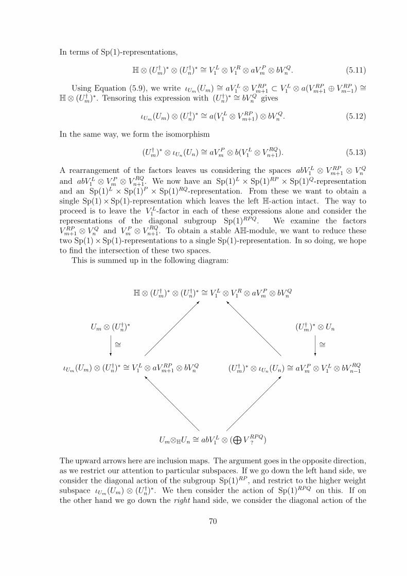
In terms of Sp(1)-representations,

H⊗ (U †m)∗ ⊗ (U †

n)∗ ∼= V L1 ⊗ V R

1 ⊗ aV Pm ⊗ bV Q

n . (5.11)

Using Equation (5.9), we write ιUm(Um) ∼= aV L1 ⊗ V RP

m+1 ⊂ V L1 ⊗ a(V RP

m+1 ⊕ V RPm−1)

∼=H⊗ (U †

m)∗. Tensoring this expression with (U †n)∗ ∼= bV Q

n gives

ιUm(Um)⊗ (U †n)∗ ∼= a(V L

1 ⊗ V RPm+1)⊗ bV Q

n . (5.12)

In the same way, we form the isomorphism

(U †m)∗ ⊗ ιUn(Un) ∼= aV P

m ⊗ b(V L1 ⊗ V

RQn+1). (5.13)

A rearrangement of the factors leaves us considering the spaces abV L1 ⊗ V RP

m+1 ⊗ V Qn

and abV L1 ⊗ V P

m ⊗ V RQn+1. We now have an Sp(1)L × Sp(1)RP × Sp(1)Q-representation

and an Sp(1)L × Sp(1)P × Sp(1)RQ-representation. From these we want to obtain asingle Sp(1)×Sp(1)-representation which leaves the left H-action intact. The way toproceed is to leave the V L

1 -factor in each of these expressions alone and consider therepresentations of the diagonal subgroup Sp(1)RPQ. We examine the factorsV RP

m+1 ⊗ V Qn and V P

m ⊗ VRQn+1. To obtain a stable AH-module, we want to reduce these

two Sp(1)×Sp(1)-representations to a single Sp(1)-representation. In so doing, we hopeto find the intersection of these two spaces.

This is summed up in the following diagram:

@@

@@

@@

@@I

@@

@@

@@

@@I

Um⊗HUn∼= abV L

1 ⊗ (⊕

V RPQ? )

ιUm(Um)⊗ (U †n)∗ ∼= V L

1 ⊗ aV RPm+1 ⊗ bV Q

n (U †m)∗ ⊗ ιUn(Un) ∼= aV P

m ⊗ V L1 ⊗ bV

RQn−1

H⊗ (U †m)∗ ⊗ (U †

n)∗ ∼= V L1 ⊗ V R

1 ⊗ aV Pm ⊗ bV Q

n

?

Um ⊗ (U †n)∗

∼=?

(U †m)∗ ⊗ Un

∼=

The upward arrows here are inclusion maps. The argument goes in the opposite direction,as we restrict our attention to particular subspaces. If we go down the left hand side, weconsider the diagonal action of the subgroup Sp(1)RP , and restrict to the higher weightsubspace ιUm(Um) ⊗ (U †

n)∗. We then consider the action of Sp(1)RPQ on this. If onthe other hand we go down the right hand side, we consider the diagonal action of the

70

subgroup Sp(1)RQ, restrict to the higher weight subspace (U †m)∗ ⊗ ιUn(Un), and then

consider the action of Sp(1)RPQ on this. At each ‘half-way stage’ we are consideringrepresentations of diagonal subgroups of different pairs of groups, and in both cases wetake the higher weight representation in a sum Vk+1 ⊕ Vk−1 and discard the Vk−1 part.Since we do this for different diagonal subgroups we expect to be left with differentsubspaces.

Using the Clebsch-Gordon formula, we obtain the two decompositions

V RPm+1 ⊗ V Q

n∼=

minm+1,n⊕j=0

V RPQm+1+n−2j and V P

m ⊗ VRQn+1∼=

minm,n+1⊕j=0

V PRQm+n+1−2j.

These decompositions contain fairly similar summands, with differences arising as theindex j approaches the region of minm,n. However, just because we have twoSp(1)RPQ-representations of the same weight, we cannot say that they are automati-cally the same subspace of H ⊗ (U †)∗ ⊗ (V †)∗. We want to know which parts end upcontributing to the final Sp(1)RPQ-representation whichever path we take. This willidentify the subspace Um⊗HUn ⊆ H⊗ (U †

m)∗ ⊗ (U †n)∗.

One thing that we can guarantee for any m,n > 0 is that the representation withhighest weight will be the same in both cases — both expressions have leading summandVm+n+1. We conjecture that this is the summand which we find in Um⊗HUn. This wouldfit well with the observation that stable AH-modules arise as representations of highestweight in decompositions of tensor products of Sp(1)-representations.

We will show that this is in fact the case, using Joyce’s dimension formulae for stableAH-modules. Here is the main result of this section:

Theorem 5.2.1 Let Um, Un be irreducible stable AH-modules. If m or n is even then

Um⊗HUn∼= Um+n.

If m and n are both odd then

Um⊗HUn∼= 4Um+n.

Proof. We have already noted that each irreducible representation of the Sp(1)M -actionon a stable AH-module U contributes 1 to the virtual dimension of U . Thus anystable AH-module of virtual dimension k must be a sum of at least k/2 and at most kirreducibles, depending on whether the irreducibles are odd or even.

We will deal with the three possible cases in turn.

Case 1(m and n both even): Let m = 2p, n = 2q. Then

dimUm = 4(p+ 1) dimU ′m = 2p+ 3 dimUn = 4(q + 1) and dimU ′

n = 2q + 3.

Using Theorem 4.1.14 we find that dimUm⊗HUn = 4(p + q + 1) and that the virtualdimension of Um⊗HUn is equal to 1. But any stable AH-module whose virtual dimensionis equal to 1 must be irreducible. The irreducible stable AH-module whose dimension

71

is 4(p + q + 1) and whose virtual dimension is 1 is V1 ⊗ V2(p+q)+1 = Um+n. HenceUm⊗HUn = Um+n.

Case 2(m even and n odd): Let m = 2p, n = 2q − 1. Then

dimUm = 4(p+ 1) dimU ′m = 2p+ 3 dimUn = 4(2q + 1) and dimU ′

n = 4(q + 1).

Using Theorem 4.1.14 we find that dimUm⊗HUn = 4(2p+ 2q + 1) and that the virtualdimension of Um⊗HUn is equal to 2. Thus Um⊗HUn must be either an even irreducibleor a sum of two odd irreducibles.

Consider the space ιUm(Um)⊗ (U †n)∗ ∼= a(V L

1 ⊗ V RPm+1)⊗ bV Q

n of Equation (5.12). Form = 2p and n = 2q − 1 this becomes

2V L1 ⊗ V RP

2p+1 ⊗ VQ2q−1∼= V L

1 ⊗ 2(V RPQ2p+2q ⊕ V

RPQ2p+2q−2 ⊕ . . .) (5.14)

The virtual dimension of the tensor product Um⊗HUn must be equal to 2, so we cannothave more than 2 of the irreducibles of the Sp(1)RPQ-action. We also need a totaldimension of 4(2p + 2q + 1). Examining Equation (5.14) we see that the only way thiscan occur is if Um⊗HUn

∼= V1 ⊗ 2V2p+2q, as all the other irreducibles of the Sp(1)RPQ-action have smaller dimension. Hence Um⊗HUn

∼= 2V1 ⊗ V2p+2q = Um+n.

Case 3 (m and n both odd): The argument is very similar to that of Case 2.Let m = 2p− 1, n = 2q − 1. Then

dimUm = 4(2p+1) dimU ′m = 4(p+1) dimUn = 4(2q+1) and dimU ′

n = 4(q+1).

Using Theorem 4.1.14 we find that dimUm⊗HUn = 16(p + q) and that the virtualdimension of Um⊗HUn is equal to 4.

Consider the space ιUm(Um)⊗ (U †n)∗ ∼= a(V L

1 ⊗ V RPm+1)⊗ bV Q

n of Equation (5.12). Form = 2p− 1 and n = 2q − 1 this becomes

4V L1 ⊗ V RP

2p ⊗ VQ2q−1∼= V L

1 ⊗ 4(V RPQ2p+2q−1 ⊕ V

RPQ2p+2q−3 + . . .). (5.15)

The only way Um⊗HUn can have a virtual dimension of four and a total dimension of16(p+ q) is if Um⊗HUn

∼= 4V1 ⊗ V2p+2q−1 = 4Um+n.

Quaternionic tensor products of more general stable AH-modules can be computedfrom this result by splitting into irreducibles and using the fact that the quaternionictensor product is distributive for direct sums.

This result is parallel to Theorem 4.5.7 applied to non-negative vector bundles. Forthe canonical sheaves O(n) over CP 1, H0(O(n)) ∼= Vn. The isomorphism O(n) ⊗OO(m) ∼= O(n + m) induces a map of cohomology groups H0(O(m)) ⊗ H0(O(n)) →H0(O(m+ n)). In terms of Sp(1)-representations, this is a map

V Pm ⊗ V Q

n∼= V PQ

m+n ⊕ VPQm+n−2 ⊕ . . .→ Vm+n.

The map in question is projection onto the irreducible of highest weight Vn+m. This isreally what this whole section has been about — the idea that the behaviour of stableAH-modules can be thoroughly and flexibly described by taking subrepresentations ofhighest weight in tensor products of Sp(1)-representations.

72

5.2.3 Tensor Products of Antistable AH-modules

It is not difficult to extend Joyce’s results for tensor products of stable AH-modules toirreducible antistable AH-modules — we can follow the same argument as in the proofof Theorem 4.1.14, since the generic properties of sums and intersections guaranteed bystability also hold if one or both of the AH-modules is irreducible and antistable.

Let U and V be antistable AH-modules with dimU = 4j, dimU ′ = 2j−r, dimV =4k and dimV ′ = 2k − s. Let A = ιU(U) ⊗ (V †)∗ and let B = (U †)∗ ⊗ ιV (V ). ThendimA = 4j(2k + s) and dimB = 4k(2j + r), so dim(H ⊗ (U †)∗ ⊗ (V †)∗) = 4(2j +r)(2k + s) > dimA + dimB. Thus in generic situations we would expect dimA ∩ B =dimU⊗HV = 0.

Suppose instead that V is stable, so now dimV ′ = 2k + s. A similar calculationshows that dimA + dimB ≥ dim H ⊗ (U †)∗ ⊗ (V †)∗ if and only if s(j + r) ≥ kr. Inthis case we might expect dimU⊗HV = dimA+ dimB − dim(H⊗ (U †)∗ ⊗ (V †)∗). Forexample, let U = U×

m = (aV1 ⊗ Vm+1)× and V = Un = bV1 ⊗ Vn+1. Then we would

expect that dim(U×m⊗HUn) = 2ab(m− n+ 2).

As in Section 5.2, we can describe what is going on in terms of diagonal actionson tensor products of Sp(1)-representations. We will illustrate the case Um⊗HU

×n . Let

Um = aV1⊗ Vm+1 and U×n = (bV1⊗ Vn+1)

×, so (U †m)∗ ∼= Vm and ((U×

n )†)∗ ∼= Vn+2. Thisgives rise to the standard descriptions

H⊗R (U †m)∗ ∼= aV L

1 ⊗ V R1 ⊗ V P

m∼= aV L

1 ⊗ (V RPm+1 ⊕ V RP

m−1)

andH⊗R ((U×

n )†)∗ ∼= bV L1 ⊗ V R

1 ⊗ VQn+2∼= bV L

1 ⊗ (V RQn+3 ⊕ V

RQn+1).

The only difference between this and equation (5.9) is that we have an antistable AH-module involved, and thus to obtain ιU×m(U×

m), we take the smaller summand of Vn+3 ⊕Vn+1. We use the Clebsch-Gordon formula to describe

ιUm(Um)⊗R ((U×n )†)∗ ∼= abV L

1 ⊗ V RPm+1 ⊗ V

Qn+2∼= abV L

1 ⊗

minm+1,n+2⊕j=0

V RPQm+n+3−2j

and

(U †m)∗ ⊗R ιU×n (U×

n ) ∼= abV L1 ⊗ V P

m ⊗ VRQn+1∼= abV L

1 ⊗

minm,n+1⊕j=0

V RPQm+n+1−2j

.

As with stable AH-modules, our task is to find which of these summands is in theintersection Um⊗HU

×n = ιUm(Um) ⊗R ((U×

n )†)∗ ∩ (U †m)∗ ⊗R ιU×n (U×

n ). This time sinceminm + 1, n + 2 = minm,n + 1, we can guarantee that the summand of smallestweight will appear in both expressions. From our dimensional arguments, we only expecta non-zero intersection if m < n + 2, in which case minm,n + 1 = m, and we wouldpredict that Um⊗HU

×n contains the summand Vn−m+1. Because its virtual dimension is

not positive, Um⊗HU×n cannot be stable. This suggests that

Um⊗HU×n∼= (abV1 ⊗ Vn−m+1)

× =

0 if m ≥ n+ 2U×

n−m n or m even and m < n+ 24U×

n−m n and m both odd and m < n+ 2.(5.16)

73

Rather than try to emulate Joyce’s (difficult) proof of Theorem 4.1.14, we will confirmthese conjectures by appealing to Quillen’s powerful results.

Proposition 5.2.2 Let Um be an irreducible stable AH-module and let U×n be an irre-

ducible antistable AH-module.If m ≥ n+ 2 then Um⊗HU

×n = 0.

If m < n+ 2 and m or n is even then Um⊗HU×n∼= U×

n−m.If m < n+ 2 and m and n are both odd then Um⊗HU

×n∼= 4U×

n−m.Let U×

m and U×n be antistable irreducible AH-modules. Then U×

m⊗HU×n = 0.

Proof. This follows from Theorem 4.5.7 (due to Quillen), using the correspondencesUm = η+(aO(m)) and U×

n = η−(aO(−n− 4)), where as usual a = 1 or 2 depending onwhether m,n are even or odd.

We can use this result about tensor products of antistable AH-modules to tell usabout AH-morphisms between stable AH-modules, using the isomorphism

HomAH(Um, Un) ∼= (U×m⊗HUn)′

of Theorem 4.2.9.

Proposition 5.2.3 Let Um and Un be stable AH-modules. Then

HomAH(Um, Un) ∼=

(aU×m−n)′ = aVm−n n ≤ m

0 n > m

where a = 4 if m and n are both odd and a = 1 otherwise.

Proof. This follows immediately by combining Theorems 4.2.9 and 5.2.2.

In particular, since U0 = H, we see that there are always AH-morphisms from Un intoH (and indeed, this is a defining property for AH-modules), but never AH-morphismsfrom H into Un unless n = 0.

Similarly, we can now see that there are always AH-morphisms from antistable AH-modules into stable AH-modules, but never AH-morphisms from stable AH-modules intoantistable AH-modules.

5.3 Semistable AH-modules and Sp(1)-representations

In this section we shall consider how the AH-module Xq fits into the picture of stableAH-modules and Sp(1)-representations. Recall from Section 4.1.3 that for q ∈ S2,Xq = H and X ′

q = p ∈ H : pq = −qp so that X†q∼= (X†

q )∗ ∼= Cq.

If we consider the dual AH-module X×q∼= (H,Cq) we see that the left-multiplication

Lq : H → H defined by Lq(p) = q · p gives an AH-isomorphism Xq∼= X×

q . Thissuggests that Theorem 4.2.9 might be particularly interesting in the case of Xq. For anyAH-module U , there is a canonical isomorphism

HomAH(Xq, U) ∼= (X×q ⊗HU)′

74

and soHomAH(X×

q , U) ∼= HomAH(Xq, U) ∼= (Xq⊗HU)′ ∼= (X×q ⊗HU)′.

Let φ : X×q → U be an AH-morphism. Then we need φ(1) = u ∈ U ′ and φ(q) ∈ U ′.

Since φ is H-linear, φ(q) = qu, and so u ∈ U ′ ∩ qU ′. It follows that

HomAH(Xq, U) ∼= (Xq⊗HU)′ ∼= U ′ ∩ qU ′. (5.17)

As noted by Joyce (see the summary in Section 4.1.3), the second of these isomorphismsis given by the map (idU ⊗Hχq) : (U⊗HXq)

′ → (U⊗HH)′ ∼= U ′.Though X ′

q is not itself an Sp(1)-representation, the subspaces Cq and X ′q = C⊥

q

are acted on by the Cartan subgroup U (1)q ⊂ Sp(1). As we shall see, taking the tensorproduct of a stable AH-module with the AH-module Xq serves to restrict attentionfrom information about Sp(1)-representations to information concerning representationsof the group U(1)q and its Lie algebra u(1)q.

Let Q = aI1 + bI2 + cI3 ∈ sp(1) with a2 + b2 + c2 = 1 and let q = ai1 + bi2 + ci3 ∈S2. Any irreducible representation of sp(1) is also a representation of the subalgebrau(1)q = 〈Q〉. The analysis of Vn as a U(1)q-representation is already familiar: it is thedecomposition of Vn into weight spaces of the operator Q : Vn → Vn. If we choose anidentification sp(1) ⊗R C = sl(2,C) such that Q = iH, this is exactly the same as thedecomposition of Vn into eigenspaces of H with weights −n,−n + 2, . . . , n − 2, n.This decomposition gives important information about the action of q on the AH-moduleUn = aV1 ⊗ Vn+1.

This is exactly what we have done in the explicit calculations of Section 5.1.3 for thecase q = i1. We define a basis 〈x,y〉 for the space V1 in such a way that Q(x) = ixand Q(y) = −iy. This also gives the left action of q ∈ Sp(1) on V1, since the actions ofq and Q coincide for this representation (see Section 1.2.1). This gives the left actionof q ∈ H on Un = aV1 ⊗ Vn+1.

The goal of this discussion is to describe the AH-module Un⊗HXq. We do this withthe aid of the following lemma. For ease of notation we work with the AH-module Un−1.

Lemma 5.3.1 The subspace U ′n−1 ∩ qU ′

n−1 is given by the sum of the weight spaces ofQ with highest and lowest possible weights.

Proof. Recall from Section 5.1.3 that

V1 ⊗ Vn =

⟨x⊗ an,x⊗ an−1b, . . . ,x⊗ abn−1,x⊗ bn

y ⊗ an,y ⊗ an−1b, . . . ,y ⊗ abn−1,y ⊗ bn

⟩,

and that the space (Un−1)′ ∼= Vn+1 is spanned by the vectors

x⊗an,x⊗an−1b+y⊗an, . . . ,x⊗an−kbk+y⊗an−k+1bk−1, . . . ,x⊗bn+y⊗abn−1,y⊗bn.

Define the basis vectors wk ≡ x⊗ an−kbk +y⊗ an−k+1bk−1, including w0 = x⊗ an andwn+1 = y ⊗ bn.

The action of H ∈ sl(2,C) is given by H(x ⊗ an−kbk) = (n − 2k + 1)x ⊗ an−kbk

and H(y ⊗ an−kbk) = (n − 2k − 1)y ⊗ an−kbk. Thus each basis vector wk is a weightvector with weight (n− 2k + 1). The two extreme vectors x⊗ an and y⊗ bn are also

75

weight vectors with weights n+ 1 and −n− 1 respectively. Note that all these weightsare different.

The left H-action of q on V1 ⊗ Vn is given by

q(x⊗ an−kbk) = ix⊗ an−kbk q(y ⊗ an−kbk) = −iy ⊗ an−kbk.

Left multiplication by q therefore preserves the weight space decomposition with respectto Q of a vector w ∈ V1 ⊗ Vn.

On the basis vectors wk = x⊗ an−kbk + y ⊗ an−k+1bk−1 we have

q(x⊗ an−kbk + y ⊗ an−k+1bk−1) = ix⊗ an−kbk − iy ⊗ an−k+1bk−1.

Since each vector wk has a different weight from all the others we have q(wk) ∈ Vn+1 ifand only if q(wk) ∈ 〈wk〉, and

q(∑

λkwk) ∈ Vn+1 ⇐⇒ λk = 0 or q(wk) ∈ Vn+1 for all k.

It is evident that

q(x⊗ an) = ix⊗ an ∈ Vn+1 and q(y ⊗ an) = −iy ⊗ an ∈ Vn+1,

but for all the other basis vectors wk,

q(wk) 6∈ 〈wk〉 and so q(wk) 6∈ Vn+1.

HenceVn+1 ∩ qVn+1 = 〈x⊗ an,y ⊗ bn〉,

the weight spaces with highest and lowest weight. Taking the σ-invariant subspace〈x⊗ an − y ⊗ bn〉 if Un−1 is an even AH-module yields the desired result for the AH-module Un−1.

Since the AH-submodule (id⊗Hχq)(Un−1⊗HXq) ⊂ Un−1 is the subspace generatedover H by U ′ ∩ qU ′, this demonstrates the main result of this section which describesUn⊗HXq as follows:

Theorem 5.3.2 Let Un = aV1⊗Vn+1 be an irreducible stable AH-module, whose eigenspacedecomposition with respect to Q ∈ sp(1) takes the form

V1 ⊗ Vn+1 =

⟨x⊗ an+1,x⊗ anb, . . . ,x⊗ abn,x⊗ bn+1

y ⊗ an+1,y ⊗ anb, . . . ,y ⊗ abn,y ⊗ bn+1

⟩.

If Un is an even AH-module then Un⊗HXq∼= Xq and

(id⊗Hχq)(Un⊗HXq) = H · 〈x⊗ an+1 − y ⊗ bn+1〉R,

where the H-action is induced by the H-action on V1.

If Un is an odd AH-module then Un⊗HXq∼= 2Xq and

(id⊗Hχq)(Un⊗HXq) = H · 〈x⊗ an+1,y ⊗ bn+1〉R = V1 ⊗ 〈an+1,bn+1〉.

Thus the quaternionic tensor product Un⊗HXq picks out the representations of ex-treme weight in the decomposition of Un into weight spaces of Q.

76

5.4 Examples and Summary of AH-modules

By now, the reader should be familiar with the ideas of quaternionic algebra. In thissection we shall briefly sum up this information, giving explicit constructions of the AH-modules which will occur most frequently in the following chapter, in the forms in whichthey occur most naturally.

Example 5.4.1 Recall the AH-module Y = (q1, q2, q3) : q1i1 + q2i2 + q3i3 = 0 ofExample 4.1.2. Since Y is stable and has virtual dimension 1, it follows that Y isirreducible and is isomorphic to U2 = V1⊗V3. A calculation shows that (Y †)∗ ∼= V2 andthat the equation q1i1 + q2i2 + q3i3 = 0 is precisely the condition for (q1, q2, q3) to lie inthe subspace V L

1 ⊗ V RM3 of H⊗ V M

2∼= V L

1 ⊗ V R1 ⊗ V M

2∼= V L

1 ⊗ (V RM3 ⊕ V RM

1 ).Consider the AH-modules

⊗kH Y , Sk

HY and ΛkHY . Using the dimension formulae of

Theorem 4.1.14 and Proposition 4.1.16, we discover that ΛnHY = 0 and that

⊗nH Y =

SnHY with dim(Sn

HY ) = 4(n + 1) and dim(SnHY )′ = 2n + 3. From this we deduce that

SnHY∼= U2n, and that all the even irreducible stable AH-modules can be realised as tensor

powers of the AH-module Y .

Example 5.4.2 [J1, Example 10.1] Let Z ⊂ H⊗ R4 be the set

Z = (q0, q1, q2, q3) : q0 + q1i1 + q2i2 + q3i3 = 0.

Then Z ∼= H3 is a left H-module. Define a real subspace Z ′ = (q0, q1, q2, q3) : qj ∈I and q0 + q1i1 + q2i2 + q3i3 = 0. Then dimZ = 12, dimZ ′ = 8 and Z is a stableAH-module.

In fact, Z is isomorphic to the first odd irreducible AH-module U1∼= 2V1 ⊗ V2. We

have (Z†)∗ ∼= R4 ∼= 2V1. The equation q0 + q1i1 + q2i2 + q3i3 = 0 is the condition for(q0, q1, q2, q3) to lie in the subspace 2V L

1 ⊗ V RM2 of H ⊗ 2V M

1∼= V L

1 ⊗ V R1 ⊗ 2V M

1∼=

2V L1 ⊗ (V RM

2 ⊕ V RM0 ).

Example 5.4.3 We can obtain the rest of the odd AH-modules as tensor products ofthose above. From Theorem 5.2.1 we know that

U2n+1 = U2n⊗HU1.

This combined with the previous examples shows that

U2n+1∼= Sn

HY⊗HZ.

Thus we have obtained all the irreducible stable AH-modules in terms of previouslyknown AH-modules. We can also use these constructions to write down formulae givingall those irreducible antistable AH-modules which are dual to stable AH-modules.

Example 5.4.4 Consider the AH-module (U,U ′) where

U = H2 and U ′ = 〈(1, 0), (i1, i2), (0, 1), (0, i1)〉.

Then (0, q) : q ∈ H is an AH-submodule of U isomorphic to Xi1 . However, there is nocomplementary AH-submodule V such that U ∼= Xi1 ⊕V , and indeed U is irreducible.

77

It is also clear that U is not semistable — nor is it the dual AH-module of any semistableAH-module. We call such an AH-module irregular.

Irregular AH-modules correspond to type (i) SK-modules of the form X n,α1 ⊕X n,−α−1

1

and torsion sheaves of the form O/mnx, where n ≥ 2. In the present case which singles

out the subfield Ci1 , we haveU ∼= η+(O/m2

0,∞).

For a general formula linking pairs of antipodal points z, σ(z) in CP 1 and complexsubfields of H see [Q, §14].

These are the only AH-modules which we do not describe in detail, for two reasons.Firstly, they are badly behaved compared to semistable and antistable AH-modules. Sec-ondly, as far as the author is aware, they do not arise naturally in geometrical situationsin the way that the other AH-modules do.

Example 5.4.5 There is one remaining irreducible to consider — the AH-module(H, 0). This trivially satisfies Definition 4.1.1, and so is an AH-module. Any AH-module whose primed part is zero is a direct sum of copies of (H, 0). It is easy to seethat for any irreducible AH-module U , U⊗H(H, 0) = 0 unless U = H, in whichcase we have H⊗H(H, 0) = (H, 0).

Though badly behaved, the AH-module (H, 0) does arise naturally in quaternionicalgebra — for example, Z⊗HH× = (H, 0). This suggests the notation

(H, 0) = U×−1,

in which case this result agrees with Theorem 5.2.2. Such notation is consistent with thesheaf description of antistable AH-modules, since we have

U×−1 = η−(2O(−3))

as expected. Thus we interpret (H, 0) as the ‘antistable part’ of 2V1 ⊗ V0. The dualspace (H,H) is of course not an AH-module, so there is no stable AH-module U−1 whichis dual to U×

−1. In spite of this we still regard U×−1 as ‘antistable’, because treating it as

an exception every time would be cumbersome.

We end this chapter with a diagram (overleaf) summarising much of our theory.

78

Figure 5.1: Irreducible AH-modules and the ratio of their dimensions.

0 14

12

34

1dimU ′/ dimU

AH-morphisms-

Quaternionic tensor products

H

Z ∼= U1

?

Y ∼= U2

?

Y × ∼= U×2

?

Z× ∼= U1

?H×

Xq and irregular

AH-modules

?U×−1 = (H, 0)

. . . . . .

U×n (3 ≤ n <∞)

. . . . . .

Un (3 ≤ n <∞)@

@@I

This describes the AH-modules we have met so far — all the finite-dimensional irre-ducible AH-modules. The quaternionic tensor product of two AH-modules is always tothe left of both of them in Figure 5.1. On the other hand, there are AH-morphisms froman AH-module into itself and any AH-modules to its right — and never from an AH-module to any AH-module to its left. These statements are closely linked by Theorem4.2.9. If U and V are irreducible stable or antistable AH-modules, this demonstratesthat that there will always be AH-morphisms from U⊗HV into U and V , but neverany AH-morphisms from U or V into U⊗HV , unless U or V is equal to H.

79

Chapter 6

Hypercomplex Manifolds

This chapter uses the quaternionic algebra developed in Chapters 4 and 5 to describehypercomplex manifolds. It is in three parts (the first of which is a summary of Joyce’swork, the other two being original). The first part (Section 6.1) summarises Joyce’stheory of q-holomorphic functions. A q-holomorphic function on a hypercomplex man-ifold M is a smooth function f : M → H which satisfies a quaternionic version ofthe Cauchy-Riemann equations. We let PM denote the AH-module of q-holomorphicfunctions on M . The q-holomorphic functions on the hypercomplex manifold H areprecisely the regular functions of Fueter and Sudbery. Because of the noncommuta-tivity of the quaternions, the product of two q-holomorphic functions is not in generalq-holomorphic. Nonetheless, q-holomorphic functions possess a rich algebraic structure.Joyce attempts to capture this using the concept of an H-algebra, a quaternionic versionof a commutative algebra over the real or complex numbers.

In the second part (Section 6.2), we use the Sp(1)-representation T ∗M ∼= 2nV1

defined by the hypercomplex structure to obtain a natural splitting of the quaternioniccotangent space of a hypercomplex manifold M , which we write H ⊗ T ∗M ∼= A ⊕ B.This is precisely a version of the splitting H ⊗ aVk

∼= aV1 ⊗ (Vk+1 ⊕ Vk−1) used in theprevious chapter to construct and describe all stable and antistable AH-modules, andthe Sp(1)-version of quaternionic algebra gives a complete description of the geometricsituation. A function f is q-holomorphic if and only if its differential df takes values inthe subspace A ⊂ H⊗ T ∗M . This is very similar to the situation in complex geometrywhere the differential of a holomorphic function takes values in the holomorphic cotangentspace Λ1,0. It follows that the subbundle A should be thought of as the q-holomorphiccotangent space of M , its complement B being the q-antiholomorphic cotangent space.

The third part (Sections 6.3 and 6.4) is about AH-bundles, which are smooth vectorbundles whose fibres are AH-modules. They can be defined over any smooth manifoldM , but are most interesting when M is hypercomplex. An AH-bundle E is said tobe q-holomorphic if it is simultaneously holomorphic with respect to the whole 2-sphereof complex structures on M . This condition is met if and only if E carries an anti-self-dual connection which is compatible with the structure of E as an AH-bundle. Wegeneralise the theory of q-holomorphic functions to that of q-holomorphic sections, sothat a q-holomorphic function is precisely a q-holomorphic section of the trivial bundleM ×H. We investigate the algebraic structure of q-holomorphic sections in some detail,showing that the q-holomorphic sections of a q-holomorphic vector bundle E form an

80

H-algebra module over PM .

6.1 Q-holomorphic Functions and H-algebras

6.1.1 Quaternion-valued functions

This section is mainly a summary of [J1, §§3,5], to which the reader is referred formore detail and proofs of the important results. Let M be a smooth manifold andlet C∞(M,H) be the vector space of smooth quaternion-valued functions on M . AnH-action on C∞(M,H) is defined by setting (q · f)(m) = q(f(m)) for all m ∈ M ,f ∈ C∞(M,H). Thus C∞(M,H) is a left H-module. What is less immediately obviousis that C∞(M,H) is an AH-module.

Lemma 6.1.1 Define a linear subspace

C∞(M,H)′ = f ∈ C∞(M,H) : f(m) ∈ I for all m ∈M = C∞(M, I).

With these definitions, (C∞(M,H), C∞(M,H)′) is an AH-module.

Proof. We use the fact that M can be embedded in C∞(M,H)† in the following way.For each m ∈M , define the ‘evaluation map’

θm : C∞(M,H)→ H by θm(f) = f(m).

Then θm(q · f) = q · θm(f), so θm ∈ C∞(M,H)×. Also, if f ∈ C∞(M, I) then θm(f) ∈ Ifor all m ∈M , so θm ∈ C∞(M,H)†.

Suppose that f ∈ C∞(M,H), and α(f) = 0 for all α ∈ C∞(M,H)†. Since θm ∈C∞(M,H)†, f(m) = 0 for all m ∈ M ; so f ≡ 0. Thus C∞(M,H) is an AH-module,by Definition 4.1.1.

This technique of linking a point m ∈M to an element of C∞(M,H)† is extremelyuseful. Joyce has used this process to reconstruct hypercomplex manifolds from theirH-algebras. Note that we have assumed no geometric structure on M other than thatof a smooth manifold.

Complex and quaternionic functions

For each q ∈ S2 let ιq : C → H be the inclusion obtained by identifying i ∈ C withq ∈ S2, so that ιq(a + ib) = a + qb. 1 For any real vector space E, the inclusion ιqextends to a map ιq : C⊗E → H⊗E given by ιq(e0 + ie1) = e0 + qe1 (for e0, e1 ∈ E ).Note that the images of ιq and ι−q are the same, but the two maps are not identical:since ιq(a+ ib) = a+ qb and ι−q(a+ ib) = a− qb, we see that ιq(z) = ι−q(z).

Let f = a + ib be a complex-valued function on M . Then for every q ∈ S2,the function ιq(f) = a + qb is a quaternion-valued function on M . In this way weobtain quaternion-valued functions from complex ones, and we shall soon see that thisconstruction can be used to obtain q-holomorphic functions from holomorphic ones.

1The map ιq will be distinguished from the inclusion map ιU of AH-modules by the use of lower-caserather than upper-case subscripts.

81

6.1.2 Q-holomorphic functions

In this section we will define q-holomorphic functions, the hypercomplex version of holo-morphic functions, and familiarise ourselves with some of their basic properties. Considerthe complex manifold (M, I). A complex-valued function f = f0 + idf1 ∈ C∞(M,C) isholomorphic (with respect to I ) if and only if f satisfies the Cauchy-Riemann equations

df0 + Idf1 = 0. (6.1)

Let (M, I1, I2, I3) be a hypercomplex manifold. Here is the definition of a q-holomorphicfunction on M .

Definition 6.1.2 Let f ∈ C∞(M,H) be a smooth H-valued function on M . Thenf = f0+f1i1+f2i2+f3i3 with fj ∈ C∞(M). The function f is said to be q-holomorphicif and only if it satisfies the Cauchy-Riemann-Fueter equations

Df ≡ df0 + I1df1 + I2df2 + I3df3 = 0.

The set of all q-holomorphic functions on M is called PM .

The term q-holomorphic is short for quaternion-holomorphic, and it is intended toindicate that a q-holomorphic function on a hypercomplex manifold is the appropriatequaternionic analogue of a holomorphic function on a complex manifold. If a function fis q-holomorphic then the function q · f is also q-holomorphic for all q ∈ H. Thus theset of q-holomorphic functions PM forms a left H-submodule of C∞(M,H). We adoptthe obvious definition for P ′M , namely

P ′M = f ∈ PM : f(m) ∈ I for all m ∈M.

So P ′M = PM ∩ C∞(M,H)′, and PM is an AH-submodule of C∞(M,H). Thus theq-holomorphic functions PM on a hypercomplex manifold M form an AH-module.

The product of two q-holomorphic functions is not in general q-holomorphic — we canobserve this simply by noting that all constant functions are trivially q-holomorphic, butPM is not even closed under right-multiplication by quaternions. Thus q-holomorphicfunctions do not form an algebra in the same sense that the holomorphic functions on acomplex manifold do.

We show that there are many interesting q-holomorphic functions on a hypercomplexmanifold M , by observing that every complex-valued function on M which is holo-morphic with respect to any complex structure Q ∈ S2 gives rise to a q-holomorphicfunction.

Lemma 6.1.3 Let q = a1i1 + a2i2 + a3i3 ∈ S2 and let Q = a1I1 + a2I2 + a3I3 be thecorresponding complex structure on M . Let f = x + iy ∈ C∞(M,C) be holomorphicwith respect to Q. Then ιq(f) = x+ qy is a q-holomorphic function.

Proof. The proof is a simple substitution. If f = x+ iy is holomorphic with respect toQ then it satisfies the Cauchy-Riemann equations dx+Q(dy) = 0, in which case

0 = dx+ (a1I1 + a2I2 + a3I3)(dy) = D(x+ a1yi1 + a2yi2 + a3yi3) = D(x+ qy).

82

So the H-valued function ιq(f) = x+ qy is q-holomorphic.

If f = x + iy ∈ C∞(M,C) is holomorphic with respect to Q, then its conjugatef = x − iy is holomorphic with respect to −Q. Does this mean that both x + qy andx − qy are q-holomorphic functions? Closer inspection shows that this is not the case— we see that

ιq(x+ iy) = ι−q(x− iy) = x+ qy.

So the holomorphic functions with respect to Q and −Q are mapped to the samefunctions when we consider their images under ι±q in C∞(M,H). We shall see that thisis a consequence of (indeed is equivalent to) the fact that the AH-modules Xq and X−q

are the same.Now, if the functions f, g ∈ C∞(M,Cq) are both holomorphic with respect to Q,

then so is fg ∈ C∞(M,Cq). By Lemma 6.1.3, ιq(f), ιq(g), and ιq(fg) = ιq(f)ιq(g)are all q-holomorphic. In this special case where the q-holomorphic functions f andg both take values in a commuting subfield of H, their product is also q-holomorphic.This is reminiscent of the situation described in Lemma 4.1.7, where two elements u ∈U and v ∈ V such that ιU(u) ∈ Cq ⊗ (U †)∗ and ιV (v) ∈ Cq ⊗ (V †)∗ define anelement u⊗Hv ∈ U⊗HV . In this case we have two well-defined ‘products’ of f andg — their quaternionic tensor product f⊗Hg ∈ PM⊗HPM and their product as Cq-valued functions fg = gf ∈ PM . This algebraic situation is described by the theory ofH-algebras.

6.1.3 H-algebras and Q-holomorphic functions

An H-algebra is a quaternionic version of an algebra over a commutative field. Let Fbe a commutative field (usually the real or complex numbers). An F-algebra is a vectorspace A over F, equipped with an F-bilinear multiplication map µ : A×A→ A whichhas certain algebraic properties. For example if µ(a, b) = µ(b, a) for all a, b ∈ A then µis said to be commutative. As we have already seen in Section 1.3, this formulation is ofno great use to us when seeking a quaternionic analogue because the non-commutativityof the quaternions makes the notion of an H-bilinear map untenable.

The axioms for an algebra over F can alternatively be written in terms of tensorproducts. The main feature of tensor algebra is that a bilinear map on the cartesianproduct A×B translates into a linear map on the tensor product A⊗FB. So our bilinearmultiplication map µ : A × A → A becomes an F-linear map µ : A ⊗F A → A. Thecommutative axiom µ(a, b) = µ(b, a) becomes µ(a⊗ b) = µ(b⊗a), so µ(a⊗ b− b⊗a) =µ(a ∧ b) = 0. Hence we obtain a ‘tensor algebra version’ of the commutative axiom,saying that µ : A⊗F A→ A is commutative if and only if Λ2A ⊆ kerµ.

Once we have reformulated our axioms in terms of tensor products and linear maps wecan translate them into quaternionic algebra, replacing ‘vector space’, ‘linear map’ and‘tensor product’ with ‘AH-module’, ‘AH-morphism’ and ‘quaternionic tensor product’.This is precisely what Joyce does, producing the following definition [J1, §5]:

Axiom H. (i) P is an AH-module.

(ii) There is an AH-morphism µP : P⊗HP → P , called the multiplicationmap.

83

(iii) Λ2HP ⊂ kerµP . Thus µP is commutative.

(iv) The AH-morphisms µP : P⊗HP → P and id : P → P com-bine to give AH-morphisms µP⊗H id and id⊗HµP : P⊗HP⊗HP →P⊗HP . Composing with µP gives AH-morphisms µP (µP⊗H id)and µP (id⊗HµP) : P⊗HP⊗HP → P . Then µP (µP⊗H id) =µP (id⊗HµP). This is associativity of multiplication.

(v) An element 1 ∈ A called the identity is given, with 1 /∈ P ′ and I·1 ⊆P ′.

(vi) Part (v) implies that if α ∈ P† then α(1) ∈ R. Thus for each a ∈ P ,1⊗Ha and a⊗H1 ∈ P⊗HP by Lemma 4.1.7. Then µP(1⊗Ha) =µP(a⊗H1) = a for each a ∈ P . Thus 1 is a multiplicative identity.

Definition 6.1.4 P is an H-algebra if P satisfies Axiom H.

Here H-algebra stands for Hamilton algebra. We also define morphisms of H-algebras:

Definition 6.1.5 Let P ,Q be H-algebras, and let φ : P → Q be an AH-morphism.Write 1P , 1Q for the identities in P ,Q respectively. We say that φ is an H-algebramorphism if φ(1P) = 1Q and µQ (φ⊗Hφ) = φ µP as AH-morphisms P⊗HP → Q.

Let M be a hypercomplex manifold. Joyce has constructed a multiplication mapµM with respect to which the q-holomorphic functions PM form an H-algebra, and suchthat for f, g ∈ C∞(M,Cq) holomorphic with respect to Q we have µ(f⊗Hg) = fg.In this way the the H-algebra PM includes the algebras of holomorphic functions withrespect to all the different complex structures on M .

Let M , N and (therefore) M ×N be hypercomplex manifolds. We define an AH-morphism φ : PM⊗HPN → PM×N . Let U and V be AH-modules. Let x ∈ U † ⊗ V †

and y ∈ U⊗HV . Then y · x ∈ H, where ‘ · ’ contracts together the factors of U † ⊗ V †

with those of (U †)∗ ⊗ (V †)∗ in U⊗HV ⊂ H⊗ (U †)∗ ⊗ (V †)∗. Define a linear map

λUV : U † ⊗ V † → (U⊗HV )† by setting λUV (x)(y) = y · x, (6.2)

for all x ∈ U † ⊗ V † and y ∈ U⊗HV . 2

Consider again the maps θm ∈ P†M of Lemma 6.1.1, which allow us to interpretpoints of m ∈ M as AH-morphisms θm : PM → H. In the same way, we can associateto each point (m,n) ∈M ×N the map θm ⊗ θn ∈ P†M ⊗P

†N . Then λPM ,PN

(θm ⊗ θn) ∈(PM⊗HPN)†.

Definition 6.1.6 We define a map φ : PM⊗HPN → C∞(M × N,H) as follows. Letf ∈ PM⊗HPN . Then λPM ,PN

(θm ⊗ θn) · f ∈ H and we define φ(f) : M × N → H bysetting

φ(f)(m,n) = λPM ,PN(θm ⊗ θn) · f.

For infinite-dimensional vector spaces U and V we define U ⊗ V to consist offinite sums of elements u ⊗ v. Thus φ(f) is a sum of finitely many smooth func-tions, and so is smooth. It is easy to see that φ(f) is q-holomorphic, since DM×N =

2See [J1, Definition 4.2], where Joyce defines this map and uses it to prove that U⊗HV is an AH-module.

84

DM(φ(f)) + DN(φ(f)) = 0, i.e. we can evaluate the derivatives in the M and Ndirections separately. It is clear that φ is H-linear and that φ(P ′M⊗HP ′N) ⊆ P ′M×N .Thus we have a canonical AH-morphism φ : PM⊗HPN → PM×N .

The second (and easier) step is to consider the case M = N , so φ : PM⊗HPM →PM×M . The diagonal submanifold Mdiag = (m,m) : m ∈M ⊂M ×M is a submani-fold of M ×M isomorphic to M as a hypercomplex manifold, and each q-holomorphicfunction on M ×M restricts to a q-holomorphic function on Mdiag. Let ρ be the re-striction map ρ : PM×M → PMdiag

; then ρ is an AH-morphism. Thus we can define anAH-morphism

µM = ρ φ : PM⊗HPM → PM . (6.3)

Here is the key theorem of this section:

Theorem 6.1.7 [J1, 5.5]. Let M be a hypercomplex manifold, so that PM is an AH-module. Let 1 ∈ PM be the constant function on M with value 1, and let µM :PM⊗HPM → PM be the AH-morphism µM = ρ φ of Equation (6.3). With thesedefinitions, PM is an H-algebra.

This statement is also true for C∞(M,H). An AH-morphism φ : C∞(M,H)⊗HC∞(N,H) → C∞(M × N,H) can be defined just as in Definition 6.1.6, and ρ isstill the obvious restriction. The q-holomorphic functions PM form an H-subalgebraof C∞(M,H), and the inclusion map id : PM → C∞(M,H) is an H-algebra morphism.

Example 6.1.8 Q-holomorphic functions on H [J1, §10].Consider the manifold H with coordinates (x0, x1, x2, x3) representing the quaternion

x0 + x1i1 + x2i2 + x3i3. Then H is naturally a complex manifold with hypercomplexstructure (I1, I2, I3) given by

I1dx2 = dx3, I2dx3 = dx1, I3dx1 = dx2 and Ijdx0 = dxj, j = 1, 2, 3. (6.4)

Consider the linear H-valued functions on H. Using the Cauchy-Riemann-FueterEquation (1.20) with the hypercomplex structure in (6.4), we find that f = q0x0 +q1x1 + q2x2 + q3x3 is q-holomorphic if and only if q0 + q1i1 + q2i2 + q3i3 = 0. Thusthe linear q-holomorphic functions on H form an AH-submodule of the set of all linearfunctions, and this submodule is isomorphic to the AH-module Z ∼= U1 of Example5.4.2.

Consider the AH-module U (k) of homogeneous q-holomorphic polynomials of degreek. The spaces U (k) are important in quaternionic analysis and are studied by Sudbery[Su, §6]. Joyce uses the dimension formulae of Proposition 4.1.16 to prove that Sk

HZ∼=

U (k). We can easily show that

SkHZ∼= (k + 1)V1 ⊗ Vk+1 =

(k + 1)Uk k even12(k + 1)Uk k odd.

This constructs not only the spaces U (k), but also their structure as Sp(1)-representations,which is crucial to Sudbery’s approach.

The space of all q-holomorphic polynomials on H is therefore given by the sum⊕∞k=0 S

kHZ, which is naturally an H-algebra. Joyce [J1, Example 5.1] calls this FZ , the

free H-algebra generated by Z , and this idea enables us to write down the multiplicationmap µH. The full H-algebra PH is constructed by adding in convergent power series.

85

6.2 The Quaternionic Cotangent Space

Let M be a complex manifold and recall the splitting C ⊗R T∗M = Λ1,0M ⊕ Λ0,1M

of Equation (2.1). A function f ∈ C∞(M,C) is holomorphic if df ∈ Λ1,0M . TheCauchy-Riemann operator is defined by ∂ = π0,1 d, and f is holomorphic if and onlyif ∂f = 0.

This section presents the quaternionic analogue of this description. Let M be ahypercomplex manifold. We show that there is a natural splitting of the quaternioniccotangent space H⊗T ∗M ∼= A⊕B. The bundle A is then the q-holomorphic cotangentspace of M . A function f ∈ C∞(M,H) is q-holomorphic if and only if df ∈ A, and theCauchy-Riemann-Fueter operator can be written δ = πB d, where πB is the naturalprojection to the subspace B ⊂ H ⊗ T ∗M . The ease with which quaternionic algebrapresents such close parallels with complex geometry could scarcely be more rewarding.

Theorem 6.2.1 Let M4n be a hypercomplex manifold and let H⊗ T ∗M be the quater-nionic cotangent bundle of M . The hypercomplex structure determines a natural splitting

H⊗ T ∗M ∼= A⊕B,

where dimA = 12n and dimB = 4n.

Proof. Recall from Section 3.2 that T ∗M ∼= 2nV1 as an Sp(1)-representation. Call thisrepresentation 2nV G

1 (since it is the action defined by the geometric structure of M ).Following the standard arguments of Chapter 5, we have a splitting

H⊗ T ∗M ∼= V L1 ⊗ V R

1 ⊗ 2nV G1

∼= 2nV L1 ⊗ (V RG

2 ⊕ V RG0 )

∼= A⊕B,

where A = 2nV L1 ⊗ V RG

2 and B = 2nV L1 ⊗ V RG

0 .

This is a situation with which we are by now very familiar. Using the theory ofChapter 5, we immediately deduce that

• The (fibres of the) subspaces A and B are AH-modules with A ∼= nU1 andB ∼= nU×

−1.

• Dim A = 12n and dimA′ = 8n, where A′ = A ∩ I ⊗ T ∗M . A is a stable AH-module.

• Dim B = 4n and dimB′ = 0, where B′ = B ∩ I ⊗ T ∗M . B is an antistableAH-module.

• The mapping A ⊕ B → H ⊗ T ∗M is an injective AH-morphism which is anisomorphism of the total spaces. It is not an AH-isomorphism because dim(A′⊕B′)is smaller than dim(I⊗ T ∗M).

86

The importance of this splitting lies partly in the following result:

Theorem 6.2.2 A function f ∈ C∞(M,H) is q-holomorphic if and only if df ∈C∞(A).

The proof of this theorem will be in two parts. Firstly, we investigate the projectionoperators πA and πB from H⊗ T ∗M onto A and B. We then show that the Cauchy-Riemann-Fueter operator can be written as πB d.

To work out projection maps to A and B we use the Casimir operator for thediagonal Sp(1)RG-action, obtained by coupling right-multiplication on H with the actionof the hypercomplex structure. The diagonal Lie algebra action is given by

I(ω) = I1(ω)− ωi1 J (ω) = I2(ω)− ωi2 K(ω) = I3(ω)− ωi3. (6.5)

Then C(ω) = (I2+J 2+K2)(ω) = −6ω−2χ(ω), where χ(ω) = I1(ω)i1+I2(ω)i2+I3(ω)i3.The operator χ satisfies the equation χ2 = 3 − 2χ, so has eigenvalues +1 and −3. Ifω is in the −3 eigenspace then we have C(ω) = 0, so ω ∈ V RG

0 . If ω is in the +1eigenspace then we have C(ω) = −8, so ω ∈ V RG

2 . Thus the subspaces A and B arethe eigenspaces of the operator χ. This enables us to write down expressions for πA

and πB such that πA + πB = 1.

Lemma 6.2.3 Projection maps πA : H⊗T ∗M → A and πB : H⊗T ∗M → B are givenby

πA(ω) =1

4(3ω+I1(ω)i1+I2(ω)i2+I3(ω)i3) πB(ω) =

1

4(ω−I1(ω)i1−I2(ω)i2−I3(ω)i3).

These maps depend only on the structure of M as a hypercomplex manifold.

Just as we defined the Dolbeault operators in Equation (2.4), we define new differ-ential operators δ and δ:

δ : C∞(M,H)→ C∞(M,A)δ = πA d and

δ : C∞(M,H)→ C∞(M,B)δ = πB d. (6.6)

Then for a function f ∈ C∞(M,H), df = δf + δf .

Proposition 6.2.4 A function f ∈ C∞(M,H) is q-holomorphic if and only if δf = 0.

Proof. Let f = f0 + f1i1 + f2i2 + f3i3 be a q-holomorphic function on M , so Df =df0 + I1df1 + I2df2 + I3df3 = 0. This is exactly the real part of the equation

4δf ≡ df − I1dfi1 − I2dfi2 − I3dfi3 = 0. (6.7)

Moreover, the three imaginary parts are the equations Ij(Df) = 0, which are satisfiedif and only if Df = 0. Thus the real equation Df = 0 is exactly the same as thequaternionic equation δf = 0.

87

It now follows that a function f is q-holomorphic if and only if df = δf ∈ C∞(M,A).This proves Theorem 6.2.2 and motivates the following definition:

Definition 6.2.5 Let M be a hypercomplex manifold and let H⊗ T ∗M ∼= A⊕ B, asin Theorem 6.2.1. Then A is the q-holomorphic cotangent space of M and B is theq-antiholomorphic cotangent space of M .

Here are some practical methods for writing the spaces A and B. Let ω = 1⊗ω0 +i1 ⊗ ω1 + i2 ⊗ ω2 + i3 ⊗ ω3. It is straightforward to verify that

ω ∈ A⇐⇒ ω0 + I1(ω1) + I2(ω2) + I3(ω3) = 0,

andω ∈ B ⇐⇒ ω0 = I1(ω1) = I2(ω2) = I3(ω3).

Let M4n be a hypercomplex manifold and let ea : a = 0, . . . , 4n − 1 be a basisfor T ∗xM such that Ib(e

4a) = e4a+b. In other words, we choose a particular isomorphismT ∗xM

∼= Hn such that the subspace 〈e4a, e4a+1, e4a+2, e4a+3〉 is a copy of H with itsstandard hypercomplex structure. With respect to this basis the fibres of A and B atthe point x are given by

Ax =∑

qaea : q4b + q4b+1i1 + q4b+2i2 + q4b+3i3 = 0 for all b = 0, . . . , n− 1

(6.8)

and

Bx =∑

qaea : q4b = −q4b+1i1 = −q4b+2i2 = −q4b+3i3 for all b = 0, . . . , n− 1

.

(6.9)Equation (6.8) is a higher dimensional version of the equation q0 + q1i1 + q2i2 + q3i3 = 0which gives the q-holomorphic cotangent space on H (Example 6.1.8). This gives anAH-isomorphism between Ax and the AH-module nZ ∼= nU1.

Let us pause for a moment to reflect on what has happened. On a complex manifold,we have a splitting of C⊗T ∗M into two spaces of equal dimension, which are conjugateto one another. On a hypercomplex manifold, we have a splitting into two subspaces,but they are not equal in size. Instead, one of them has three times the dimension of theother, because the subspaces are defined by the equation V1 ⊗ V1

∼= V2 ⊕ V0. This typeof splitting into spaces of dimension 3n and n is typical of the quaternions, echoing thefundamental isomorphism H ∼= I⊕ R.

6.2.1 The Holomorphic and Q-holomorphic cotangent spaces

Let M4n be a hypercomplex manifold with hypercomplex structure (I1, I2, I3). Letq = a1i1 +a2i2 +a3i3 ∈ S2 and let Q = a1I1 +a2I2 +a3I3 be the corresponding complexstructure on M . We have already seen (Lemma 6.1.3) that if f is a complex-valuedfunction on M which is holomorphic with respect to the complex structure Q, thenιq(f) is a q-holomorphic function. This is a correspondence not only of holomorphicand q-holomorphic functions, but also of the holomorphic and q-holomorphic cotangentspaces.

88

Each complex structure Q on M defines a holomorphic cotangent space Λ1,0Q . Using

the embedding ιq we can consider C⊗T ∗M ∼= Cq⊗T ∗M as a subspace of H⊗T ∗M . Therelationship between these subspaces of H⊗ T ∗M is clarified in the following Lemma:

Lemma 6.2.6 Let A ⊂ H ⊗ T ∗M be the q-holomorphic cotangent space of a hyper-complex manifold M and let Λ1,0

Q ⊂ C⊗ T ∗M be the holomorphic cotangent space withrespect to the complex structure Q. Then

H · ιq(Λ1,0Q ) = (idA⊗Hχq)(A⊗HXq).

Proof. We illustrate the case dimM = 4, the general result holding in exactly thesame way but involving more coordinates. For any point x ∈ M we choose a basise0, e1, e2, e3 for T ∗xM such that the hypercomplex structure at x is given by thestandard relations (6.4). Without loss of generality take q = i1 and consider the complexmanifold (M, I1). Then

Λ1,0I1

= 〈e0 + ie1, e2 + ie3〉C.Since ιi1(a+ ib) = a+ i1b, we see that

H · ιq(Λ1,0I1

) = H · 〈e0 + i1e1, e2 + i1e

3〉. (6.10)

Recall from Section 5.3 that (idU ⊗Hχq)(U⊗HXq)′ = U ′ ∩ qU ′ for any AH-module

U . Using Equation (6.8), we have A = (q0e0 + . . .+ q3e3) : q0 + q1i1 + q2i2 + q3i3 = 0

and A′ = I⊗ T ∗M . It follows that

A′ ∩ i1A′ = q0e0 + . . .+ q3e3 ∈ A : qj ∈ 〈i2, i3〉

= 〈i2e0 − i3e1, i3e0 + i2e1, i2e

2 − i3e3, i3e2 + i2e3〉, (6.11)

and the image (idA⊗Hχi1)(A⊗HXi1)∼= 2Xi1 is generated over H by this subspace.

Observe that −i2 · (i2e0 − i3e1) = e0 + i1e

1 and that −i2 · (i2e2 − i3e3) = e2 + i1e

3.Therefore H · (A′ ∩ i1A′) is exactly the same as the subspace H · ιq(Λ1,0

I1) of Equation

(6.10).

This gives us a description of the q-holomorphic and q-antiholomorphic cotangentspaces of M in terms of complex geometry:

Corollary 6.2.7 Let M4n be a hypercomplex manifold, with q-holomorphic cotangentspace A and q-antiholomorphic cotangent space B. Then

A =∑Q∈S2

H · ιq(Λ1,0Q )

andB =

⋂Q∈S2

H · ιq(Λ0,1Q ).

Thus the q-holomorphic cotangent space is generated over H by the different holomorphiccotangent spaces.

Proof. Use the fact that A is a stable AH-module; thus A is generated over H by thesubspaces A′ ∩ qA′ for q ∈ I. The proof now follows immediately from Lemma 6.2.6.

89

6.3 AH-bundles

An AH-bundle is the natural quaternionic analogue of a real or complex vector bundle:a set of AH-modules E parametrised smoothly by a base manifold M .

Definition 6.3.1 Let M be a differentiable manifold and (W,W ′) a fixed AH-module. A smooth AH-module bundle with fibre W or simply AH-bundle is a family(Ex, E

′x)x∈M of AH-modules parametrised by M , together with a differentiable man-

ifold structure on E =⋃

x∈M Ex such that

• The projection map π : E →M , π : Ex 7→ x is C∞.

• For every x0 ∈ M , there exists an open set U ⊆ M containing x0 and a diffeo-morphism

φU : π−1(U)→ U ×Wsuch that φ(Ex) 7→ x ×W is an AH-isomorphism for each x ∈ U .

A section of an AH-bundle is a smooth map α : M → E such that α(x) ∈ Ex forall x ∈ M , and the left H-module of smooth sections of E is denoted by C∞(M,E).Define C∞(M,E)′ = C∞(M,E ′). With this definition, it is easy to adapt Lemma 6.1.1to show that if E is an AH-bundle then C∞(M,E) is an AH-module. We can multiplysections on the left by quaternion-valued functions, and C∞(M,E) is a left module overthe ring C∞(M,H).

The standard real or complex algebraic operations which give new bundles from oldcan be transfered en masse to quaternionic algebra and AH-bundles. Let (E, π1,M) and(F, π2, N) be AH-bundles. We define a bundle (E⊗HF,M×N) by setting (E⊗HF )(m,n) =Em⊗HFn. We can define a bundle E ⊕ F in the same way.

In particular, let E and F be AH-bundles over M . By restricting to the diago-nal submanifold of M ×M we define a bundle (E⊗HF,M) by setting (E⊗HF )m =Em⊗HFm. In the same way (E ⊕ F,M), Λk

HE and SkH(E) are AH-bundles, as is E×

if the fibres of E are SAH-modules. We will always make clear whether an AH-bundle‘E⊗HF ’ refers to (E⊗HF,M ×M) or the diagonal restriction (E⊗HF,M).

The q-holomorphic and q-antiholomorphic cotangent bundles A and B are bothAH-bundles, and are AH-subbundles of H ⊗ T ∗M . In fact, every AH-bundle can beregarded as an AH-subbundle of some bundle H⊗ V , as is easy to demonstrate:

Lemma 6.3.2 Let E = (E, π,M) be an AH-bundle. Then E is isomorphic to anAH-subbundle of H⊗ V , for some real vector bundle (V, π1,M).

Proof. This is an extension of the fact that any AH-module W is isomorphic to ιW (W ) ⊆H ⊗ (W †)∗. Consider the map ιEx(Ex) : Ex → H⊗ (E†

x)∗ for x ∈ M . Let Vx = (E†

x)∗.

Then V =⋃

x∈M Vx is a real vector bundle, and H ⊗ V is an AH-bundle. Thus E isisomorphic to the AH-subbundle ⋃

x∈M

ιEx(Ex) ⊆ H⊗ V,

and the lemma is proved.

90

Abusing notation slightly, if E is an AH-bundle we will often write ιE : E →H⊗ (E†)∗ for the set of inclusion maps

⋃x∈M(ιEx : Ex → H⊗ (E†

x)∗).

We could broaden our definition of an AH-bundle, demanding only that E should bea real vector bundle possessing a left H-action and a real subbundle E ′ such that (Ex, E

′x)

is an AH-module for all x ∈M . The following example shows why this definition wouldbe unwieldy:

Example 6.3.3 Let M = R, and define a real vector bundle E = R×H. Define a realsubspace E ′ ⊂ E by

E ′x = 〈i1, i2 + xi3〉.

It is easy to check that (Ex, E′x) = Xi3−xi2 as an AH-module. Thus E is not an AH-

bundle, since the fibres Ex and Ey are not AH-isomorphic for x 6= y. There is goodreason for excluding E from being an AH-bundle. For example,

(E⊗HXi3)x =

Xi3 if x = 00 otherwise.

So despite the fact that E is a smooth vector bundle, E⊗HXq is not; if we consideredthis broader class of objects to be ‘AH-bundles’ then they would not be closed under thetensor product.

Let V be a real vector bundle over the manifold M with fibre Rk, and let P V

be the bundle of frames associated with V . Then P V is a principal bundle with fibreGL (k,R), and V = P V ×GL(k,R) Rk. In the same way, let E be an AH-bundle with fibreW and let G = AutAH(W ). We can define a principal G-bundle PE associated withE so that E = PE ×G W . As we know, G will be a subgroup of GL (k,H). In mostcases, G will be significantly smaller than GL (k,H). For example, if W = U2j for somej then by Theorem 4.2.9 we have HomAH(U2j, U2j) ∼= R, so AutAH(U2j) = R∗ = R \ 0and PE is just a principal R∗-bundle. Principal bundles associated with AH-bundlestend to be much smaller than those associated with real or complex vector bundles.

6.3.1 Connections on AH-bundles

Definition 6.3.4 Let E be an AH-bundle over M . An AH-connection on E is anAH-morphism

∇E : C∞(M,E) −→ C∞(M,E ⊗ T ∗M) = Ω1(M,E)

which satisfies the rule∇E(f · α) = df ⊗ α+ f · ∇Eα

for all α ∈ C∞(M,E), f ∈ C∞(M,H).

We will sometimes omit the subscript and just write ‘∇ ’ when the AH-bundle Eis clearly implied. Let ∇ be an AH-connection on E. Then the map id⊗(∇†E)∗ isan AH-connection on H⊗ (E†)∗ which preserves ιE(E). Thus every AH-connection ∇on E is equivalent to a connection (∇†)∗ on the real vector bundle (E†)∗. We will notdistinguish between ∇ and (∇†)∗, but will write ∇ for both. This equivalence allows usto construct AH-connections on tensor products, in very much the same way that Joyceconstructs the AH-morphism φ⊗Hψ from AH-morphisms φ and ψ [J1, Definition 4.4].

91

Lemma 6.3.5 Let (E,M) and (F,N) be AH-bundles and let ∇E and ∇F be AH-connections on E and F . Then ∇E and ∇F induce an AH-connection ∇E⊗HF on theAH-bundle (E⊗HF,M ×N).

Proof. We regard ∇E as a connection on (E†)∗. The bundle ((E†)∗,M) extendstrivially to a bundle ((E†)∗,M × N) over M × N . Using the natural identificationT ∗(m,n)(M ×N) ∼= T ∗mM ⊕ T ∗nN , define a differential operator ∇E,M on ((E†)∗,M ×N),where ∇E,M differentiates only in the M -directions of M ×N . In the same way definea connection ∇F,N on ((F †)∗,M × N) which differentiates only in the N -directions.Adding these gives a differential operator

∇E,M ⊗ id + id⊗∇F,N : C∞((E†)∗ ⊗ (F †)∗) −→ C∞((E†)∗ ⊗ (F †)∗ ⊗ T ∗(M ×N)).

This operator is a connection on the real vector bundle (E†)∗ ⊗ (F †)∗, so the operatorid⊗(∇E,M ⊗ id + id⊗∇F,N) on the bundle (H ⊗ (E†)∗ ⊗ (F †)∗,M × N) is an AH-connection.

Since ∇E is an AH-connection, the operator id⊗∇E,M⊗id maps sections of ιE(E)⊗(F †)∗ to sections of ιE(E)⊗ (F †)∗⊗T ∗(M ×N), and acts trivially on the (F †)∗ factor;thus id⊗∇E,M ⊗ id maps sections of E⊗HF to sections of E⊗HF ⊗ T ∗(M ×N). Thesame is true for id⊗ id⊗∇F,N , and so the AH-connection id⊗(∇E,M ⊗ id + id⊗∇F,N)preserves the AH-subbundle (E⊗HF,M×N), on which it is therefore an AH-connection.We call this connection ∇E⊗HF .

If E and F are AH-bundles over the same manifold M we can use Lemma 6.3.5 todefine an AH-connection on the diagonal bundle (M,E⊗HF ).

This process can be described in terms of principal bundles. 3 Suppose that φ ∈AutAH(W ) for some AH-module W . Then φ induces a real linear isomorphism (φ×)∗ :(W †)∗ → (W †)∗. In this way the action of G = AutAH(W ) on W gives rise to an actionon (W †)∗. Let E be an AH-bundle with fibre W , and let P be the associated principalbundle with fibre G, so that E = P ×G W . An AH-connection ∇E on E gives riseto a connection DP on the principal bundle P , and vice versa. Since connections onprincipal bundles always exist, we can use this to guarantee that every AH-bundle hasan AH-connection.

Let F be another AH-bundle with fibre V , let H = AutAH(V ) and let Q be theassociated principal bundle with fibre H, so that F = Q×H V . An AH-connection ∇F

on F gives rise to a connection DQ on the principal bundle Q. Consider the principalbundle P × Q, a bundle over M × N with fibre G ×H. Since G acts on (W †)∗ andH acts on (V †)∗, there is an induced action of G × H on W⊗HV . The AH-bundle(E⊗HF,M ×N) is the associated bundle (P ×Q)×G×H W⊗HV . Since the connectionsDP and DQ define a unique connection DP ⊕DQ on the product bundle P ×Q, thisgives rise to a connection on the associated bundle E⊗HF . Since G × H acts as AH-automorphisms on W⊗HV , this induced connection is an AH-connection, which we canidentify with the AH-connection ∇E⊗HF of Lemma 6.3.5.

3A similar discussion for connections in complex vector bundles can be found in [K, §1.5].

92

6.4 Q-holomorphic AH-bundles

Using complex geometry as a model, we define a q-holomorphic AH-bundle over ahypercomplex manifold M to be one which is holomorphic with respect to each complexstructure Q ∈ S2. An AH-bundle is q-holomorphic if and only if it admits a connectionwhose curvature takes values only in E2,0 = Λ2

−. We define the q-holomorphic sections ofa q-holomorphic vector bundle using a version of the Cauchy-Riemann-Fueter equations.Q-holomorphic sections have interesting algebraic properties, which generalise those ofJoyce’s q-holomorphic functions. We give an interpretation of q-holomorphic sections interms of quaternionic algebra and the q-holomorphic cotangent space, which makes thestep-by-step correspondence with complex geometry extremely clear.

Here is the main definition of this section:

Definition 6.4.1 Let E be an AH-bundle over the hypercomplex manifold M , equippedwith an AH-connection ∇. Suppose that ∇ gives E the structure of a holomorphicvector bundle over the complex manifold (M,Q) for all Q ∈ S2. Then (E,∇) is aq-holomorphic AH-bundle.

If we want to be really specific we can write (E, π,M,∇) for our q-holomorphicbundle; on the other hand, if a connection is already specified, we can simply refer tothe total space E as a q-holomorphic AH-bundle. The existence of such a connectionensures that the different holomorphic structures are compatible. A lot can be learnedabout q-holomorphic AH-bundles by studying the connection ∇.

6.4.1 Anti-self-dual connections and q-holomorphic AH-bundles

Let E be a complex vector bundle over the complex manifold (M, I) and let ∇ bea connection on E. Just as we split the exterior differential d = ∂ + ∂, we can define

∂E = π1,0∇ : C∞(E)→ C∞(E⊗Λ1,0M) and ∂E

= π0,1∇ : C∞(E)→ C∞(E⊗Λ0,1M).

Proposition 6.4.2 The connection ∇ gives E the structure of a holomorphic vector

bundle if and only if ∂E ∂E

= 0, i.e. the (0, 2)-component of the curvature R of∇ vanishes. Conversely, if E is a holomorphic vector bundle then E admits such aconnection.

Proof. This is Propositions 3.5 and 3.7 of [K, p. 9].

Let E be a q-holomorphic AH-bundle over the hypercomplex manifold M , so E hasthe structure of a holomorphic vector bundle over (M,Q) for every complex structureQ ∈ S2. Let ∇ be a connection on E and let R be the curvature of ∇. Each

Q ∈ S2 defines a splitting ∇ = ∂EQ +∂

E

Q, and so a decomposition of the curvature tensor

R = R2,0Q + R1,1

Q + R0,2Q . By Proposition 6.4.2, ∇ defines a holomorphic structure on

E with respect to Q if and only if R0,2Q ≡ 0. If we reverse the sense of Q then we

reverse the decomposition of R, so R0,2−Q = R2,0

Q . Thus ∇ gives E the structure of a

holomorphic vector bundle with respect to every Q ∈ S2 if and only if R2,0Q = R0,2

Q = 0for all Q ∈ S2, i.e. the curvature of ∇ is of type (1, 1) with respect to all Q ∈ S2.

93

A 2-form ω is of type (1, 1) with respect to every Q ∈ S2 if and only if it isannihilated by the action of sp(1) on Λ2T ∗M , so ω ∈ E2,0 ⊂ Λ2T ∗M . By analogywith the 4-dimensional theory (see Example 3.2.6), we call E2,2 the space of self-dual2-forms Λ2

+ and E2,0 the space of anti-self-dual 2-forms Λ2−. A connection ∇ whose

curvature R takes values only in C∞(End(E)⊗E2,0) is therefore called an anti-self-dualconnection.

Several authors have considered self-dual and anti-self-dual connections, particularyon quaternionic Kahler manifolds: for example Galicki and Poon [GP], Nitta [N] andMamone Capria and Salamon [MS]. This is partly because such connections give minimaof a Yang-Mills funtional on M . It is important to note that Mamone Capria andSalamon refer to the bundle E2,0 as self-dual rather than anti-self-dual, and so referto connections taking values in E2,0 as self-dual connections. There is no unanimousconvention in the literature: our choice is made because we are using the conventionsthat Ij(e

0) = ej not −ej, and that the volume form e0123 gives a positive orientation ofH.

We have established the following result:

Theorem 6.4.3 Let E be an AH-bundle over the hypercomplex manifold M equippedwith an anti-self-dual AH-connection nabla. Then (E,∇) is a q-holomorphic AH-bundle.

Conversely, an AH-bundle E equipped with an AH-connection ∇ is q-holomorphicif and only if ∇ is anti-self-dual.

This is similar to the idea of hyperholomorphic bundles described by Verbitsky [V, §2].Verbitsky considers the case where B is a Hermitian vector bundle over a hyperkahlermanifold, so the fibres of such a bundle are not normally H-modules. There is no reasonwhy his definition cannot be extended to hypercomplex manifolds, since as we have seen,the Hermitian inner product is not necessary to force the connection to be anti-self-dual if it is to be compatible with the 2-sphere of holomorphic structures. If E is aq-holomorphic AH-bundle then it is easy to see that H ⊗ (E†)∗ is also q-holomorphic,and (E†)∗ ⊗ C is a hyperholomorphic bundle. Conversely, if B is a hyperholomorphicbundle with a real structure σ such that B = Bσ⊗C, then H⊗Bσ is a q-holomorphicAH-bundle. Any AH-subbundle E of H⊗ Bσ which is preserved by the anti-self-dualconnection ∇ will also be q-holomorphic.

The following Proposition gives further insight into the analogy between holomorphicand q-holomorphic bundles:

Proposition 6.4.4 Let (E, π,M,∇) be a q-holomorphic AH-bundle over the hypercom-plex manifold M . Then E is itself a hypercomplex manifold.

Proof. Consider the splitting of TE into horizontal and vertical subbundles TE ∼=E ⊕ TM , where the vertical subbundle E is naturally defined by the structure of E asan AH-bundle and the horizontal subbundle TM is defined by the connection.

Define a hypercomplex structure (I1, I2, I3) on TE as follows. On the verticalsubbundle isomorphic to E, the action of I1, I2 and I3 is given by the fixed left H-actionof i1, i2 and i3 on the fibres. On the horizontal subbundle isomorphic to TM , define

94

the hypercomplex structure (I1, I2, I3) to be the horizontal lift of the hypercomplexstructure on M . This defines an almost-hypercomplex structure on E. The integrabilityof this structure is guaranteed by the fact that (E, Ij) is a holomorphic vector bundlefor j = 1, 2, 3.

Example 6.4.5 Let M be a hypercomplex manifold. Then the Obata connection∇ on T ∗M is anti-self-dual and defines an anti-self-dual AH-connection on H⊗ T ∗M ,which is thus a q-holomorphic AH-bundle. Let A ⊂ H ⊗ T ∗M be the q-holomorphiccotangent space of M,

A = ω0 + i1 ⊗ ω1 + i2 ⊗ ω2 + i3 ⊗ ω3 : ω0 + I1ω1 + I2ω2 + I3ω3 = 0, ωj ∈ T ∗M.

Let a = a0+i1a1+i2a2+i3a3 ∈ C∞(M,A). Then ∇a0+I1(∇a1)+I2(∇a2)+I3(∇a3) = 0(where I1, I2 and I3 act on the A factor of A⊗T ∗M ), since ∇Ij = 0 for j = 1, 2, 3. Itfollows that ∇a ∈ C∞(A⊗T ∗M). Hence the Obata connection defines an AH-connectionon A. Since the Obata connection is anti-self-dual, A is a q-holomorphic AH-bundle.

Example 6.4.6 Let E and F be q-holomorphic AH-bundles. Then so are the var-ious associated bundles E⊗HF , E ⊕ F , Λk

HE and so on, all with their induced AH-connections.

6.4.2 Q-holomorphic sections

Q-holomorphic sections of AH-bundles are defined using a version of the Cauchy-Riemann-Fueter equations. We cannot automatically rewrite Equation (6.7) to define a Cauchy-Riemann-Fueter operator on a general AH-bundle E, because the fibres of E will notin general have a well-defined right H-action. Instead, we use the inclusion map ιE tomanipulate sections of e in a more manageable form.

Definition 6.4.7 Let E be an AH-bundle over the hypercomplex manifold M equippedwith an AH-connection ∇. Let e ∈ C∞(M,E) so that ιE(e) = e0 + i1e1 + i2e2 + i3e3,ej ∈ C∞(M, (E†))∗. Then e is a q-holomorphic section of E if and only if

∇e0 + I1(∇e1) + I2(∇e2) + I3(∇e3) = 0, (6.12)

where I1, I2 and I3 act on the T ∗M factor of E ⊗ T ∗M .Let P(M,E) = P(E) be the space of q-holomorphic sections of E. Let P(E)′ =

P(E) ∩ C∞(M,E ′) so that P(E) is an AH-submodule of C∞(M,E).

Q-holomorphic sections are the natural generalisation of q-holomorphic functions,which are precisely the q-holomorphic sections of the trivial bundle M × H equippedwith the flat connection. So PM = P(M ×H).

A general AH-bundle might have no q-holomorphic sections. However, if the AH-bundle (E,∇) is q-holomorphic then E is holomorphic with respect to the complexstructure Q, and admits holomorphic sections. It is easy to adapt Lemma 6.1.3 toshow that the holomorphic sections of this holomorphic vector bundle give rise to q-holomorphic sections of E.

95

Not all q-holomorphic AH-bundles have interesting q-holomorphic sections. For ex-ample, the q-antiholomorphic cotangent space B ⊂ H⊗T ∗M is closed under the actionof the Obata connection, and so is technically a q-holomorphic AH-bundle. Recall that

B = ω − i1 ⊗ I1(ω)− i2 ⊗ I2(ω)− i3 ⊗ I3(ω) : ω ∈ T ∗M.

Let b = b0 − i1I1b0 − i2I2b0 − i3I3b0 ∈ C∞(M,B), so b is q-holomorphic if and only if

∇b0 − I1∇I1b0 − I2∇I2b0 − I3∇I3b0 = 0.

Since ∇Ij = 0 and I2j = −1, this equation is satisfied if and only if ∇b = 0, and the

AH-bundle B admits no non-trivial q-holomorphic sections. In fact, this follows fromthe fact that B′ = 0, and such behaviour is predicted and described by the algebra ofthe quaternionic cotangent space.

Q-holomorphic sections and the quaternionic cotangent space

Let E be a q-holomorphic AH-bundle over the hypercomplex manifold M . We candescribe the q-holomorphic sections of E using the q-holomorphic cotangent space, justas we did for q-holomorphic functions in the previous chapter. The inclusion map ιEand the AH-connection ∇ (regarded as a connection on (E†)∗ ) define an AH-morphism∇ ιE : C∞(M,E) → C∞(M,H ⊗ (E†)∗ ⊗ T ∗M). After swapping the H and (E†)∗

factors, we have a copy of the quaternionic cotangent space H ⊗ T ∗M , which we cansplit into the q-holomorphic and q-antiholomorphic spaces A and B. Thus we have amap ∇ ιE : C∞(M,E) → C∞(M, (E†)∗ ⊗ (A ⊕ B)). We can now use the projectionsπA and πB of the previous chapter to split the action of ∇ ιE into two operators.

Definition 6.4.8 Let (E,∇) be a q-holomorphic AH-bundle. We define the pair ofoperators δE : C∞(E)→ C∞((E†)∗ ⊗ A) and δE : C∞(E)→ C∞((E†)∗ ⊗B) by

δE = (id(E†)∗ ⊗πA) ∇ ιE

andδE = (id(E†)∗ ⊗πB) ∇ ιE.

Hence we regard E as a subspace of H ⊗ (E†)∗, and then the action of ∇ on Esplits into a q-holomorphic part δE and a q-antiholomorphic part δE so that in effect∇ = δE + δE. This is an exact analogue of the complex case where a connection ∇splits as ∇ = π1,0 ∇ + π0,1 ∇. Let V be a holomorphic vector bundle with a

connection ∇ compatible with the holomorphic structure, so that ∂E

= ∂. A sectionv ∈ C∞(V ) is holomorphic if and only if π0,1 ∇(s) = 0. In just the same way, theoperator e 7→ ∇e0 + I1(∇e1) + I2(∇e2) + I3(∇e3) of Definition 6.4.7 is precisely the realpart of δE, and a section e ∈ C∞(E) is q-holomorphic if and only if δE(e) = 0.

This analogy goes further. In complex geometry, a section v ∈ C∞(V ) is holomorphicif and only if ∂v = 0, which means that ∇v ∈ C∞(V ⊗CΛ1,0M). Here is the quaternionicanalogue of this statement:

96

Proposition 6.4.9 Let (E, π,M,∇) be a q-holomorphic AH-bundle, and let e ∈ C∞(E)be a q-holomorphic section. Then

∇ ιE(e) ∈ C∞(E⊗HA),

where A is the q-holomorphic cotangent space of M .

Proof. Let e be q-holomorphic, so δE(e) = 0 and ∇ ιE(e) = δE(e) ∈ C∞(H⊗ (E†)∗⊗T ∗M). Using the identification (A†)∗ ∼= T ∗M we can regard δE(e) as a section ofH⊗ (E†)∗ ⊗ (A†)∗.

The induced connection ∇ on (E†)∗ preserves ιE(E), so δE(e) ∈ C∞(ιE(E)⊗(A†)∗).Clearly δE(e) ∈ C∞((E†)∗ ⊗ ιA(A)), since δE is defined by projection to this subspace.Thus ∇ ιE(e) ∈ C∞(E⊗HA), by Definition 4.1.4.

In complex geometry, a holomorphic section v of a holomorphic vector bundle V isone whose covariant derivative ∇v takes values in the complex tensor product of V withthe holomorphic cotangent space. In hypercomplex geometry, a q-holomorphic section eof a q-holomorphic vector bundle E is one whose covariant derivative ∇e takes valuesin the quaternionic tensor product of E with the q-holomorphic cotangent space.

6.4.3 Sections of Tensor Products

For real and complex vector bundles, there is a natural inclusion C∞(M,E)⊗C∞(N,F )→ C∞(M×N,E⊗F ) given by (e⊗f)(m,n) = e(m)⊗f(n). The quaternionic analogueof this map is more delicate. Let E and F be AH-bundles. We want to define an AH-morphism φ : C∞(M,E)⊗HC

∞(N,F ) → C∞(M × N,E⊗HF ). The obvious difficultyis that for sections e and f of E and F respectively, there will not in general be asection e⊗Hf of the AH-bundle (E⊗HF,M × N). Instead we use a generalisation ofJoyce’s map φ : PM⊗HPN → PM×N (Definition 6.1.6).

Consider first the fibres Em and Fn for m ∈ M and n ∈ N . Let α ∈ E†m and

β ∈ F †n. Define an AH-morphism αm : C∞(M,E) → H by αm(e) = α(e(m)) for all

e ∈ C∞(M,E). Then αm ∈ C∞(M,E)†. Similarly, define the ‘evaluation at n ∈ N ’,βn(f) = β(f(n)). Then βn ∈ C∞(N,F )†. The operators αm and βm are generalisationsof Joyce’s θm ∈ C∞(M,H)†, introduced in Lemma 6.1.1. With H-valued functions(sections of M × H ), the evaluation map θm generates the whole of H†

m∼= R. For

more general AH-bundles, we need to consider the combination of a point m at whichto evaluate sections, and an AH-morphism α ∈ E†

m, since we can no longer assume thatthe map α = id generates the whole of E†

m.For AH-modules U and V , recall the linear map λUV : U † ⊗ V † → (U⊗HV )† of

Equation (6.2). Thus there are linear maps λEm,Fn : E†m ⊗ F †

n → (Em⊗HFn)† andλC∞(M,E),C∞(N,F ) : C∞(M,E)† ⊗ C∞(N,F )† → (C∞(M,E)⊗HC

∞(N,F ))†.

Definition 6.4.10 Let ε ∈ C∞(M,E)⊗HC∞(N,F ). Define φE,F (ε)(m,n) ∈ Em⊗HFn

by the equation

λEm,Fn(α⊗ β) · φE,F (ε)(m,n) = λC∞(M,E),C∞(N,F )(αm ⊗ βn) · ε

for all m ∈M , α ∈ E†m and for all n ∈ N , β ∈ F †

n.

97

Thus φE,F (ε) defines a section of the AH-bundle (E⊗HF,M × N). By the samearguments as in Definition 6.1.6, φE,F (ε) is smooth because it is a finite sum of smoothsections, and so we have a linear map

φE,F : C∞(M,E)⊗HC∞(M,F )→ C∞(M ×N,E⊗HF ).

It is easy to see that φE,F is an injective AH-morphism. We shall call φE,F the sectionproduct map for AH-bundles.

If e ∈ C∞(M,E) and f ∈ C∞(N,F ) satisfy the conditions of Lemma 4.1.7 (so ifιE(e) and ιF (f) both take values in Cq for some q ∈ S2) then the section φE,F (e⊗Hf) isthe complex product of the sections, so φ(e⊗Hf)(m,n) = e(m)⊗Hf(n) ∼= e(m)⊗Cq f(n).The section product map is the natural tool for relating tensor products of sections withsections of tensor products and allows us to treat sections of more complicated AH-bundles using similar techniques to those used by Joyce for q-holomorphic functions.

It is well known that sums and tensor products of holomorphic sections are themselvesholomorphic. The same is true for sums of q-holomorphic sections, and there is ananalogous description for q-holomorphic sections of quaternionic tensor products, usingthe section product map φE,F . This is a generalisation of the fact (Definition 6.1.6) thatφ : PM⊗HPN → PM×N .

Theorem 6.4.11 Let (E, π1,M,∇E) and (F, π2, N,∇F ) be q-holomorphic AH-bundles,and let P(M,E) ⊂ C∞(M,E) and P(N,F ) ⊂ C∞(N,F ) be the AH-modules of theirq-holomorphic sections. Then

φE,F : P(M,E)⊗HP(N,F ) −→ P(M ×N,E⊗HF ),

where E⊗HF is equipped with the connection ∇E⊗HF , so the section product map takesq-holomorphic sections to q-holomorphic sections.

Proof. Consider the anti-self-dual connection ∇E⊗HF = id⊗(∇E,M ⊗ id + id⊗∇F,N).Then ∇E⊗HF = δE⊗HF + δE⊗HF . Using the natural splitting T ∗(M ×N) ∼= T ∗M ⊕T ∗N ,we see that δE⊗HF = δE,M⊗id + id⊗δF,N , where δE,M differentiates sections of ιE(E) inthe M directions and then projects to the q-antiholomorphic cotangent space of M×N ,and similarly for δF,N .

Let ε ∈ P(E)⊗HP(F ), and let φE,F (ε) ∈ C∞(M×N,E⊗HF ), where φE,F is the sec-tion product map of Definition 6.4.10. Since ε ∈ ιP(E)(P(E))⊗ (P(F )†)∗, it follows that(δE,M⊗id)(φE,F (ε)) = 0. Similarly, (id⊗δF,N)(φE,F (ε)) = 0. Hence δE⊗HF (φE,F (ε)) = 0,and φE,F (ε) is q-holomorphic.

Just as for q-holomorphic functions, when M = N we can restrict to the diagonalbundle (E⊗HF,M). The restriction map ρ clearly preserves q-holomorphic sections,and we obtain a natural product ρ φE,F : P(M,E)⊗HP(M,F ) → P(M,E⊗HF ). Inparticular, let E be a q-holomorphic AH-bundle over M , let P(E) be the AH-moduleof q-holomorphic sections of E and let PM = P(H) be the H-algebra of q-holomorphicfunctions on M . Then by Theorem 6.4.11, we have a natural AH-morphism

ρ φH,E : PM⊗HP(E) −→ P(H⊗HE) ∼= P(E). (6.13)

We can descibe such an algebraic situation by saying that P(E) is an H-algebra moduleover PM . Here is the definition of an H-algebra module:

98

Axiom M. (i) Q is an AH-module and (P , µP) is an H-algebra.

(ii) There is an AH-morphism µQ : P⊗HQ → Q, called the modulemultiplication map.

(iii) The maps µP and µQ combine to give AH-morphisms µP⊗H id andid⊗HµQ : P⊗HP⊗HQ → P⊗HQ. Composing with µQ gives AH-morphisms µQ (µP⊗H id) and µQ (id⊗HµQ) : P⊗HP⊗HQ → Q.Then µQ(µP⊗H id) = µQ(id⊗HµQ). This is associativity of modulemultiplication.

(iv) For u ∈ Q, 1⊗Hu ∈ P⊗HQ by Lemma 4.1.7. Then µQ(1⊗Hu) = ufor all u ∈ Q. Thus 1 acts as an identity on Q.

Definition 6.4.12 Q is an H-algebra module if Q satisfies Axiom M.

The idea of an H-algebra module was suggested by Joyce, and the axioms follow avery similar pattern to those for an H-algebra (Definition 6.1.4). It is relatively easyto see that the q-holomorphic sections P(E) of a q-holomorphic AH-bundle form anH-algebra module over the H-algebra PM , the module multiplication map being thesection product map φH,E of Equation (6.13). The proof of this statement is obtainedby adapting Joyce’s proof that the q-holomorphic functions PM form an H-algebra [J1,Theorem 5.5].

One possible application of this idea is to study anti-self-dual connections (instantons)on H. Different connections will give rise to different H-algebra modules of q-holomorphicsections. This suggests that the theory of H-algebra modules over PH might lead to analgebraic description of instantons on H.

99

Chapter 7

Quaternion Valued Forms andVector Fields

This final chapter uses the algebra and geometry developed so far to describe quaternion-valued tensors on hypercomplex manifolds. On a hypercomplex manifold we have globalcomplex structures, which allows us to adapt the real-valued double complex of Chapter3 to decompose quaternion-valued forms. The splitting H ⊗ T ∗M ∼= A ⊕ B of theprevious chapter is the first example of this type of decomposition. More generally, forall k and r we obtain a splitting of H⊗Ek,r into two AH-bundles. This decompositiongives rise to a double complex of quaternion-valued forms on hypercomplex manifolds,which has some advantages over the real-valued double complex. Not only the top rowbut the top two rows of the quaternion-valued double complex are elliptic, and in fourdimensions the whole complex is elliptic. The top row of the quaternion-valued doublecomplex is particularly well-behaved, and can be constructed using quaternionic algebra.This allows us to define q-holomorphic k-forms, and to describe their algebraic structureusing ideas from the previous chapter.

A similar approach to quaternion-valued vector fields is also fruitful. Just as withthe quaternionic cotangent space, there is a splitting of the quaternionic tangent spaceH⊗ TM using which we define a hypercomplex version of the ‘(1, 0) vector fields’ on acomplex manifold. These vector fields are closed under the Lie bracket (suitably adaptedto the quaternionic situation). This encourages us to adapt the axioms for a Lie algebrato form a quaternionic version, in a similar way to that in which Joyce arrived at H-algebras. The Lie bracket on hypercomplex manifolds defines a natural operation onvector fields which satisfies these axioms.

In recent times, Spindel et al. [SSTP] and Joyce [J3] demonstrated the existence of in-variant hypercomplex structures on certain compact Lie groups and their homogeneousspaces. This discovery presents us with lots of examples of finite-dimensional quater-nionic Lie algebras. We use this idea to calculate the quaternionic cohomology groups ofthe group U(2), and suggest how these methods may be extended to higher-dimensionalhypercomplex Lie groups.

100

7.1 The Quaternion-valued Double Complex

In Chapter 3, we saw how the real-valued exterior forms ΛkT ∗M on a quaternionicmanifold M are acted upon by the principal Sp(1)-bundle Q of local almost complexstructures on M . Recall that the subbundle of ΛkT ∗M consisting of Vr-type represen-tations is denoted Ek,r = εn

k,rVr.Suppose in addition that M is hypercomplex, and so possesses global complex struc-

tures I1, I2 and I3 = I1I2 (in other words, Q is the trivial bundle M×Sp(1) ). Insteadof just real or complex forms (which we can think of as taking values in the trivial repre-sentation V0), consider forms taking values in some Sp(1)-representation W , i.e. sectionsof the bundle W ⊗ΛkT ∗M . Since the Sp(1)-action on ΛkT ∗M is now defined by globalcomplex structures, we can take the diagonal action under which the subspace W ⊗Ek,r

splits according to the Clebsch-Gordon formula.The situation in which we are particularly interested is that of forms taking values

in the quaternions H = V L1 ⊗ V R

1 . As suggested in Section 3.4, we obtain splittings bycoupling the right Sp(1)-action on H with the Sp(1)-action on ΛkT ∗M . In symbols, thistakes the form

H⊗ Ek,r∼= V L

1 ⊗ V R1 ⊗ εn

k,rVGr∼= εn

k,rVL1 ⊗ (V RG

r+1 ⊕ V RGr−1). (7.1)

Proposition 7.1.1 Let M4n be a hypercomplex manifold. The AH-bundle H⊗ΛkT ∗Mdecomposes as

H⊗ ΛkT ∗M ∼= V L1 ⊗

(k+1⊕r=0

(εnk,r+1 + εn

k,r−1)VRGr

),

where r ≡ k + 1 mod 2.

Proof. By Proposition 3.2.1, we have

H⊗ ΛkT ∗M ∼= V L1 ⊗ V R

1 ⊗

(k⊕

r=0

εnk,rV

Gr

),

where the ‘Sp (1)G-action’ is the action of Sp(1) on ΛkT ∗M induced by the hypercomplexstructure. Taking the diagonal Sp(1)RG-action using the Clebsch-Gordon formula, thisbecomes

H⊗ ΛkT ∗M ∼= V L1 ⊗

(k⊕

r=0

εnk,r(V

RGr+1 ⊕ V RG

r−1)

). (7.2)

Collecting together the Vr representations yields the formula in the Proposition.

Definition 7.1.2 Define Fk,r to be the subspace (εnk,r+2 +εn

k,r)V1⊗Vr+1 ⊆ H⊗ΛkT ∗M .

The primed part of the space Fk,r is obtained using the theory of Chapter 5. As inEquation 5.10, Equation 7.1 is a decomposition of H ⊗ Ek,r into stable and antistableAH-modules. (This is a generalisation of the splitting H ⊗ T ∗M ∼= A ⊕ B.) DefiningF ′

k,r = Fk,r ∩ (I ⊗ ΛkT ∗M), the space Fk,r is an AH-subbundle of H ⊗ (F †k,r)

∗ = H ⊗

101

(Ek,r+2 ⊕ Ek,r), and each (fibre of the) AH-bundle Fk,r is the direct sum of stable andantistable components. The splitting

H⊗ Ek,r∼= εn

k,rVL1 ⊗ (V RG

r+1 ⊕ V RGr−1)

gives an H-module isomorphism

H⊗ Ek,r∼=

εn

k,rUr ⊕ εnk,rU

×r−2 for r even

12εn

k,rUr ⊕ 12εn

k,rU×r−2 for r odd.

(7.3)

As with the decomposition H⊗T ∗M ∼= A⊕B, these are not AH-isomorphisms becausesome of the primed part is lost in the splitting. We give names to these spaces as follows(where as usual a = 1 if n is even and a = 2 if n is odd):

Definition 7.1.3 Define F ↑k,r to be the AH-bundle 1

aεn

k,rUr ⊆ H ⊗ Ek,r. Define F ↓k,r

to be the AH-bundle 1aεn

k,r+2U×r ⊆ H ⊗ Ek,r+2. Thus F ↑

k,r is the Ur-type subspace of

H⊗ ΛkT ∗M and F ↓k,r is the U×

r -type subspace of H⊗ ΛkT ∗M , so that

Fk,r = F ↑k,r ⊕ F

↓k,r.

The q-holomorphic cotangent space A is F1,1 = F ↑1,1 and the q-antiholomorphic cotan-

gent space B is F1,−1 = F ↓1,−1.

With these definitions, we have (F ↑k,r

†)∗ = (F ↓

k,r−2

†)∗ = Ek,r, and H ⊗ Ek,r

∼= F ↑k,r ⊕

F ↓k,r−2. Just as with the splitting H⊗T ∗M ∼= A⊕B, there is an injective AH-morphism

F ↑k,r ⊕ F

↓k,r−2 → H⊗ Ek,r

which is an H-linear isomorphism of the total spaces but is not injective on the primedparts. A short calculation shows that

dimF ↑k,r = 2(r + 2)εn

k,r

dimF ↑k,r

′= (r + 3)εn

k,r

anddimF ↓

k,r = 2(r + 2)εnk,r+2

dimF ↓k,r

′= (r + 1)εn

k,r+2.

Since we can consider the bundles F ↑k,r and F ↓

k,r separately, it may appear strangeto mix up the stable and antistable fibres in the single bundle Fk,r. However, it soonbecomes clear that exterior differentiation does not necessarily map stable fibres to stablefibres or antistable fibres to antistable fibres, so in order to obtain a double complex itis necessary to amalgamate the stable and antistable contributions.

The definition of the operators δ and δ of Section 6.2 can now be generalised tocover the whole of H ⊗ Λ•T ∗M , giving rise to a double complex of quaternion-valuedforms.

Definition 7.1.4 Let πk,r be the natural projection map πk,r : H ⊗ ΛkT ∗M → Fk,r.Define the differential operators δ, δ : Ωk(M,H)→ Ωk+1(M,H) by

δ : C∞(Fk,r)→ C∞(Fk+1,r+1)δ = πk+1,r+1 d

andδ : C∞(Fk,r)→ C∞(Fk+1,r−1)δ = πk+1,r−1 d .

102

Theorem 7.1.5 The exterior derivative d maps C∞(M,Fk,r) to C∞(M,Fk+1,r+1 ⊕Fk+1,r−1), so

d = δ + δ.

It follows thatδ2 = δδ + δδ = δ2 = 0.

and the decomposition H⊗ ΛkT ∗M =⊕k+1

r=0 Fk,r gives rise to a double complex.

Proof. The proof works in exactly the same way as that of Theorem 3.2.3. Let ∇ bethe Obata connection on M , so ∇ : C∞(M,Fk,r)→ C∞(M,Fk,r ⊗ T ∗M). Since

Fk,r ⊗ T ∗M = (εnk,r+2 + εn

k,r)V1 ⊗ Vr+1 ⊗ 2nV1,

it follows (from the Clebsch-Gordon splitting Vr+1 ⊗ 2nV1∼= 2n(Vr+2 ⊕ Vr), followed by

the antisymmetrisation d = ∧∇ ) that d : C∞(M,Fk,r)→ C∞(M,Fk+1,r+1⊕Fk+1,r−1).The rest of the theorem follows automatically.

Figure 7.1: The Quaternion-Valued Double Complex

C∞(M,F0,0 = H)

*

HHHH

HHj

δ

δ

C∞(M,F1,1 = A)

*

HHHHH

Hj

δ

δ

C∞(M,F1,−1 = B)

*

δ

C∞(M,F2,0)

*

HHHH

HHj

δ

δ

C∞(M,F2,2)

*

HHHHH

Hj

δ

δ

C∞(M,F3,1)

*

HHHHH

Hj

δ

δ

C∞(M,F3,3)HHH

HHHj

δ

. . . . . . etc.

C∞(M,F3,−1)

*

δ

. . . . . . etc.

As already hinted, the operators δ and δ do not preserve stable or antistable sub-spaces. For example, though we have δ : Fk,r → Fk+1,r−1, it is not the case that

δ : F ↑k,r → F ↑

k+1,r−1. This can be observed in the simplest of cases — a quaternion-valued

function f is a section of F0,0 = F ↑0,0, and unless f is q-holomorphic δf is a nonzero

section of F ↓1,−1.

Much of the theory from the real-valued double complex of Chapter 3 can be adaptedto describe the quaternion-valued version as well. For example, the operators δ and δcan be expressed in a similar fashion to D and D, using the Casimir element techniqueof Lemma 3.2.7. The Casimir operator in question is that of the diagonal Lie algebraaction given by the operators

I(ω) = I1(ω)− ωi1 J (ω) = I2(ω)− ωi2 K(ω) = I3(ω)− ωi3.

103

of Equation (6.5). This leads to the following adaptation of Lemma 3.2.7:

Lemma 7.1.6 Let α ∈ C∞(Fk,r). Then

δα = −1

4

(r +

1

r + 2(I2 + J 2 +K2)

)dα

and

δα =1

4

((r + 4) +

1

r + 2(I2 + J 2 +K2)

)dα.

The results on ellipticity in Section 3.3 can also be adapted to the new situation. Wecan infer that the operator δ is elliptic except at the bottom spaces F2k−1,−1 and F2k,0.Again, the operator δ is elliptic at some of these lowest-weight spaces for low exteriorpowers; in particular the leading edge of spaces Fk,k forms a complex which is ellipticthroughout. Closer examination also reveals that the ‘second row’ of spaces Fk,k−2 isalso an elliptic complex with respect to δ.

Lemma 7.1.7 The complex

0 −→ C∞(F1,−1)δ−→ C∞(F2,0)

δ−→ . . .δ−→ C∞(F2n+1,2n−1)

δ−→ 0

is elliptic.

Proof. Ellipticity at C∞(Fk,k−2) for all k ≥ 3 follows from a generalisation of thetechniques used in the proof of Theorem 3.3.1. We need to show that the complex iselliptic at C∞(F1,−1) = C∞(B) and C∞(F2,0). As in Section 3.3, it is enough to choosesome e0 ∈ T ∗M and show that the symbol sequence

0 −→ F1,−1σ−→ F2,0

σ−→ F3,1σ−→ . . . etc.

is exact, where σ(ω) = σδ(ω, e0) = πk+1,r+1(ωe

0) for ω ∈ Fk,r. (As usual ωe0 meansω ∧ e0.)

Since δ = d on F1,−1 = B, we have σ(β) = βe0 for all β ∈ B. It follows from theexpression for B in Equation (6.9) that σ : B → F2,0 is injective, so the complex iselliptic at B.

Let ω ∈ F2,0. Then σ(ω) = 0 if and only if ωe0 ∈ F3,−1, which is the case if andonly if I(ωe0) = J (ωe0) = K(ωe0) = 0. The first of these equations is

I1(ωe0)− ωe0i1 = I1(ω)e0 + ωe1 − ωe0i1 = 0.

It follows by taking exterior product with e0 that ωe10 = 0. The same arguments forJ and K show that

σ(ω) = 0 =⇒ ωe10 = ωe20 = ωe30 = 0,

and so ωe0 must be equal to zero and ω = γe0 for some γ ∈ H⊗ T ∗M .

104

It remains to show that we can choose β ∈ B such that ω = βe0. Suppose insteadthat ω = αe0, with α ∈ A. Since the complex is elliptic at A it follows that αe0 ∈ F2,0

if and only if α = σ(q) = 14q(3e0 + e1i1 + e2i2 + e3i3) for some q ∈ H. But then

αe0 = βe0, where β = 14q(−e0 + e1i1 + e2i2 + e3i3) ∈ B. Hence we can find β ∈ B such

that σ(ω) = 0 implies that ω = σ(β) for all ω ∈ F2,0, so the complex is exact at F2,0.This completes the proof.

This is an unexpected bonus — on hypercomplex manifolds, the double complex ofquaternion-valued forms has not just one but two rows which with respect to the operatorδ are elliptic throughout, namely the top row Fk,k and the second row Fk,k−2.

Example 7.1.8 Quaternion-valued forms in four dimensions

Figure 7.2: The Quaternion-Valued Double Complex in Four Dimensions

F0,0 = H

*

HHHH

HHj

δ

δ

A ∼= Z

*

HHHH

HHj

δ

δ

B ∼= U×−1

*

δ

F2,0∼= 3H⊕H×

*

HHHHHHj

δ

δ

Λ2HA∼= Y

HHHHH

Hjδ

F3,1∼= Z

HHHH

HHjδ

F3,−1∼= U×

−1

*

δ

F4,0∼= H

In four dimensions the situation is particularly friendly towards quaternion-valuedforms, because the whole double complex is elliptic. To show this, choose a standardbasis of 1-forms e0, . . . , e3 for T ∗M so that as usual Ij(e

0) = ej. Explicitly, we haveH⊗ T ∗M ∼= F1,1 ⊕ F1,−1, where

F1,1 = A = q0e0 + q1e1 + q2e

2 + q3e3 : q0 + q1i1 + q2i2 + q3i3 = 0,

F1,−1 = B = q0e0 + q1e1 + q2e

2 + q3e3 : q0 = q1i1 = q2i2 = q3i3.

Next, H⊗ Λ2T ∗M ∼= F2,2 ⊕ F2,0, where

F2,2 = Λ2HA = q1e01+23 + q2e

02+31 + q3e03+12 : q1i1 + q2i2 + q3i3 = 0,

F2,0 = F ↑2,0 ⊕ F

↓2,0

= 〈e01−23, e02−31, e03−12〉H ⊕ q1e01+23 + q2e02+31 + q3e

03+12 : q1i1 = q2i2 = q3i3.

Lastly, H⊗ Λ3T ∗M ∼= F3,1 ⊕ F3,−1, where

F3,1 = q0e123 + q1e032 + q2e

013 + q3e021 : q0 + q1i1 + q2i2 + q3i3 = 0,

F3,−1 = q0e123 + q1e032 + q2e

013 + q3e021 : q0 = q1i1 = q2i2 = q3i3.

It follows that the symbol map σδ is an isomorphism between F3,−1 and F4,0, and soin four dimensions the entire quaternion-valued double complex is elliptic.

105

7.1.1 The Top Row ΛkHA and Q-holomorphic k-forms

In contrast with the the role of the Cauchy-Riemann operator ∂ in the Dolbeault com-plex, the Cauchy-Riemann-Fueter operator δ in the quaternion-valued double complex(Figure 7.1) does not begin a longer elliptic complex. 1 On the other hand, the operatorδ on functions does extend to give the elliptic complex

0 −→ C∞(F0,0)δ−→ C∞(F1,1)

δ−→ . . .δ−→ C∞(F2n,2n)

δ−→ 0.

This section discusses these top row spaces Fk,k which are of particular interest.In complex geometry the Hodge decomposition of forms results immediately from the

isomorphism C⊗T ∗M ∼= Λ1,0⊕Λ0,1 and the isomorphism in exterior algebra Λk(U⊕V ) =⊕p+q=k ΛpU ⊗ ΛqV . With hypercomplex geometry we are not quite so lucky, since the

splitting A ⊕ B ∼= H ⊗ T ∗M is not an AH-isomorphism but rather an injective AH-morphism which is not surjective on the primed parts. Despite the fact that we canidentify H⊗ ΛkT ∗M with Λk

H(H⊗ T ∗M), the induced AH-morphism

ιk : ΛkH(A⊕B) → H⊗ ΛkT ∗M

is therefore not an isomorphism for k > 1. This is why we resort to our more complicatedanalysis of the Sp(1)-representation on H⊗ΛkT ∗M to discover the quaternionic versionof the Dolbeault complex. In spite of this, the inclusion map ιk is still of special interest,because it describes explicitly the top row of the double complex.

Proposition 7.1.9 Let A be the q-holomorphic cotangent space of a hypercomplex man-ifold M . The inclusion map ιk : Λk

H(A⊕B) → H⊗T ∗M identifies ΛkHA with the highest

space Fk,k ⊆ H⊗ ΛkT ∗M .

Proof. There is a natural identification ΛkH(A⊕B) =

⊕p+q=k(Λ

pHA⊗HΛq

HB), and so

ιk :⊕

p+q=k

ΛpHA⊗HΛq

HB → H⊗ ΛkT ∗M.

Since B′ = 0, B⊗HB = 0 and so ΛkHB = 0 for k > 1 ; also A⊗HB = 0. Thus

ΛkH(A ⊕ B) = Λk

HA for k > 1, and the map ιk : ΛkH(A ⊕ B) → H ⊗ ΛkT ∗M is none

other than the normal inclusion map ι : ΛkHA → H ⊗ (Λk

HA†)∗. It follows that there is

an AH-submodule of H⊗ ΛkT ∗M which is isomorphic to ΛkHA.

Now, A ∼= nU1, so by Theorem 5.2.1, ΛkHA ⊆

⊗kHA∼= mUk for some m. (Recall

that Uk = aV1 ⊗ Vn+1 where a = 1 for k even and a = 2 for k odd.) By Proposition4.1.16, dim Λk

H(nU1) = 2(k + 2)(2nk

). It follows that

ΛkHA∼=

1

a

(2n

k

)Uk =

(2n

k

)V1 ⊗ Vk+1. (7.4)

Thus ιk(ΛkHA) must be a subspace of H⊗ ΛkT ∗M of this form.

1In 1991, Baston [Bas] succeeded in extending the Cauchy-Riemann-Fueter operator to a locallyexact complex with a different construction involving second order operators.

106

From Definition 7.1.2, we see that Fk,k =(2nk

)V1 ⊗ Vk+1 as well. Since there are no

other representations of this weight in H⊗ ΛkT ∗M , it follows that

ιk(ΛkHA) = Fk,k,

so there is a natural isomorphism ιk : ΛkHA∼= Fk,k.

Just as we define the q-holomorphic cotangent space A as being a particular sub-module of H ⊗ T ∗M , so that (A†)∗ = T ∗M , we identify its exterior powers with thecorresponding AH-submodules of H ⊗ ΛkT ∗M . Thus we will omit to write the ‘ ιk ’,writing Λk

HA = Fk,k and (ΛkHA

†)∗ = Ek,k.In Section 6.2.1 we showed that the q-holomorphic cotangent space A is generated

over H by the various holomorphic cotangent spaces (Corollary 6.2.7). We generalisethis result to higher exterior powers as follows:

Theorem 7.1.10 2 Let A be the q-holomorphic cotangent space of a hypercomplex man-ifold M4n. Then

(id⊗Hχq)(ΛkHA⊗HXq) = H · ιq(Λk,0

Q ).

It follows that

ΛkHA =

∑Q∈S2

H · ιq(Λk,0Q ),

i.e. the space ΛkHA is generated over H by the spaces of (k, 0)-forms Λk,0

Q .

Proof. Since ΛkHA∼=(2nk

)V1 ⊗ Vk+1, it follows that Λk

HA⊗HXq∼=(2nk

)Xq. This is AH-

isomorphic to the submodule (id⊗Hχq)(ΛkHA⊗HXq) ⊂ Λk

HA, which by Theorem 5.3.2 isgenerated over H by the weight-spaces of Q with extremal weight.

Consider the weights of the action of Q ∈ S2 ⊂ sp(1). The highest-weight vectors inC⊗ ΛkT ∗M are the (k, 0)-forms Λk,0

Q , which are mapped to Cq ⊗ ΛkT ∗M by the map

ιq. Thus H · ιq(Λk,0Q ) ⊂ (id⊗Hχq)(Λ

kHA⊗HXq), and since dimC Λk,0

Q =(2nk

)we see that

H · ιq(Λk,0Q ) = (id⊗Hχq)(Λ

kHA⊗HXq),

proving the first part of the Theorem.Since Λk

HA is stable, it is generated by these subspaces. The result follows.

Just as the q-holomorphic cotangent space A is our quaternionic analogue of theholomorphic cotangent space T ∗1,0M , the AH-bundle Λk

HA is the quaternionic analogueof the bundle of (k, 0)-forms Λk,0 = Λk

CT∗1,0M . Both are formed in the same way using

exterior algebra over their respective fields, and both form the ‘top row’ of their doublecomplexes. This suggests a natural definition of a ‘q-holomorphic k-form’:

Definition 7.1.11 Let M be a hypercomplex manifold. A quaternion-valued k-formω ∈ Ωk(M,H) is q-holomorphic if and only if ω ∈ C∞(M,Λk

HA) and δω = 0. TheAH-module of q-holomorphic k-forms on M will be written Pk

M , so the H-algebra ofq-holomorphic functions on M is P0

M = PM .

2This theorem is really a quaternionic version of (Salamon’s) Equation 2.10, which is essentially thesame result for complexified k-forms.

107

This gives rise to what we may call the q-holomorphic de Rham complex

0 −→ PMd=δ−→ P1

Md=δ−→ P2

Md=δ−→ . . .

d=δ−→ P2n−1M

d=δ−→ P2nM

d=δ−→ 0. (7.5)

Just as (on a complex manifold) Λk,0 is a holomorphic vector bundle, it is easy tosee that (Λk

HA,∇) is a q-holomorphic AH-bundle where ∇ is (the connection inducedby) the Obata connection on M . The q-holomorphic k-forms Pk

M are precisely the q-holomorphic sections P(Λk

HA) of the AH-bundle (ΛkHA,∇) as introduced in Definition

6.4.7, as the following Proposition demonstrates:

Proposition 7.1.12 A quaternion-valued k-form ω ∈ C∞(M,ΛkHA) satisfies the

equation δω = 0 if and only if ∇ω ∈ C∞(ΛkHA⊗HA), i.e. ω is a q-holomorphic section

of (ΛkHA,∇).

Proof. The ‘if’ part is automatic, since ∇ω ∈ C∞(ΛkHA⊗HA) implies that dω = ∧∇ω ∈

C∞(Λk+1H A) and so δω = 0.

The reverse implication is nontrivial and depends upon analysing the Sp(1)-representation on Λk

HA⊗ T ∗M . Using Equation (7.4), we have

ΛkHA⊗ T ∗M ∼=

(2n

k

)V L

1 ⊗ V Mk+1 ⊗ 2nV G

1

∼= 2n

(2n

k

)V L

1 ⊗ (V MGk+2 ⊕ V MG

k ).

The bundle ΛkHA⊗HA is precisely the higher-weight subspace 2n

(2nk

)V L

1 ⊗ V GHk+2 . The

complementary subspace 2n(2nk

)V L

1 ⊗ V GHk is revealed by Proposition 7.1.1 to be none

other than the bundle Fk+1,k−1 ⊂ H⊗ Λk+1T ∗M . The component of ∇ω taking valuesin Fk+1,k−1 is of course δω, the vanishing of which therefore guarantees that ∇ω ∈C∞(Λk

HA⊗HA).

The q-holomorphic de Rham complex therefore inherits a a rich and interesting alge-braic structure. We have already noted that d : Pk

M → Pk+1M . It follows from the theory

of q-holomorphic sections that q-holomorphic forms are closed under the tensor product.Explicitly, let

φΛkHA,Λl

HA : C∞(M,ΛkHA)⊗HC

∞(M,ΛlHA) −→ C∞(M ×M,Λk

HA⊗HΛlHA)

be the section product map (Definition 6.4.10). Define φk,l to be the restriction toC∞(M,Λk+l

H A), brought about by the restriction ρ : M × M → M to the diagonalsubmanifold Mdiag ⊂M ×M followed by the skewing map ∧ : C∞(M,Λk

HA⊗HΛlHA)→

C∞(M,Λk+lH A). It follows (from Theorem 6.4.11 and Proposition 7.1.12) that

φk,l : PkM⊗HP l

M −→ Pk+lM .

Thus the H-algebra structure on the q-holomorphic functions PM extends to oneon the q-holomorphic k-forms P•M , and we say that P•M forms a differential gradedH-algebra. It is well known that on a real or complex manifold M one can use exteriorproducts over R or C to give an algebraic structure to de Rham or Dolbeault cohomology,which is often called the cohomology algebra of M . It may be that the differential gradedH-algebra structure on P•M can be used to give a similar description of the quaternioniccohomology of a hypercomplex manifold.

108

7.2 Vector Fields and Quaternionic Lie Algebras

Quaternionic algebra can also be used to describe vector fields on a hypercomplex man-ifold M . Using similar ideas to those of Section 6.2, we define a splitting of the quater-nionic tangent space H ⊗ TM ∼= A ⊕ B. Quaternion-valued vector fields which takevalues in the subspace A ⊂ H ⊗ TM turn out to be a good hypercomplex analogue ofthe ‘ (1, 0) vector fields’ in complex geometry. In particular, an almost hypercomplexstructure is integrable if and only if these vector fields are closed under a quaternionicversion of the Lie bracket operator. This encourages us to treat these vector fields as aquaternionic Lie algebra, a new concept which we proceed to define and explore.

7.2.1 Vector Fields on Hypercomplex Manifolds

As so often, we take our inspiration from complex geometry. An almost complex structureI on a manifold M defines a splitting C ⊗ TM ∼= T 1,0M ⊕ T 0,1M , where T 1,0M isthe holomorphic and T 0,1M the antiholomorphic tangent space of M . Let V be theset of smooth vector fields on M . The Lie bracket is a bilinear map from V × V toV . Let V1,0 = C∞(M,T 1,0M) be the vector fields of type (1, 0) on M . The almostcomplex structure I is integrable if and only if the Lie bracket preserves (1, 0) vectorfields, which is expressed by the inclusion

[V1,0,V1,0] ⊆ V1,0. (7.6)

The obstruction to this equation is the Nijenhuis tensor NI which measures the (0, 1)component of the Lie bracket of two (1, 0) vector fields.

We present a similar theorem for quaternionic vector fields on hypercomplex mani-folds. Let M4n be a hypercomplex manifold. We define a splitting of the quaternionictangent space H ⊗ TM , which is roughly dual to the splitting H ⊗ T ∗M ∼= A ⊕ B ofSection 6.2.

Definition 7.2.1 Let M4n be a hypercomplex manifold so that TM ∼= 2nV1 as anSp(1)-representation. The quaternionic tangent space H ⊗ TM splits according to theequation

H⊗ TM ∼= V L1 ⊗ V R

1 ⊗ 2nV G1∼= 2nV L

1 ⊗ (V RG2 ⊗ V RG

0 ).

Define the AH-subbundles A = 2nV L1 ⊗ V RG

2 and B = 2nV L1 ⊗ V RG

0 , using the natural

definitions A′ = A ∩ (I ⊗ TM) and B′ = B ∩ (I ⊗ TM) = 0. Then A is the

q-holomorphic tangent bundle and B is the q-antiholomorphic tangent bundle of M .

This definition is perfectly natural, though not quite ideal from the point of view ofquaternionic algebra. We would like A and B to be dual to the cotangent spaces Aand B. However, whilst there are H-linear bundle isomorphisms A ∼= A× and B ∼= B×,these spaces are not isomorphic as AH-bundles, nor is there any fruitful way to alter thedefinitions to make them so.

The Lie bracket of vector fields is a bilinear map [ , ] : V × V → V , and so definesa natural linear map λ : V ⊗ V → V . As with H-algebras, we will find it much moremeaningful to talk about linear maps on tensor products, and we can use this formulationto obtain a quaternionic analogue of Equation (7.6).

109

Definition 7.2.2 Let M be a hypercomplex manifold with q-holomorphic tangentspace A ⊂ H ⊗ TM . Let V = C∞(M,TM) be the vector space of smooth real vectorfields on M .

Define VH = H⊗ V to be the AH-module of smooth quaternion-valued vector fieldson M , so VH = C∞(M,H⊗ TM). Define VA = C∞(M, A) to be the AH-submodule of

H-valued vector fields on M taking values in A ⊂ H ⊗ TM . We will refer to elementsof VA as A-type vector fields.

The relationship between these vector fields and the map λ : V ⊗ V → V is par-ticularly interesting. Using the canonical isomorphism (H ⊗ TM)⊗H(H ⊗ TM) ∼=H ⊗ TM ⊗ TM , the Lie bracket defines an AH-morphism (which we shall also callλ )

λ : VH⊗HVH → VH,

which is effectively a Lie bracket operation on quaternionic vector fields.Here is the quaternionic version of Equation (7.6). The formulation and proof is

similar in spirit to Theorem 6.4.11.

Theorem 7.2.3 Let M be a hypercomplex manifold with q-holomorphic tangent spaceA, and let VA denote the space of A-type vector fields on M . Then the Lie bracket λon quaternionic vector fields preserves VA, so that

λ : VA⊗HVA → VA.

Proof. To begin with, we use the section product map φA,A (Definition 6.4.10) to regard

elements of VA⊗HVA as sections in C∞(A⊗HA) ⊂ C∞(H⊗ TM ⊗ TM).

Let vj, wj ∈ V be vector fields such that∑

j qj⊗vj⊗wj ∈ C∞(A⊗HA), which meansthat

∑qj ⊗ vj,

∑qj ⊗wj ∈ VA. We want to find an expression for λ(

∑qj ⊗ vj ⊗wj) =∑

qj ⊗ [vj, wj].

The Obata connection ∇ is an AH-connection on A (and in fact is anti-self-dual, so

that A is a q-holomorphic AH-bundle). Thus ∇(∑qj ⊗ wj) is an element of C∞(A⊗

T ∗M). Contracting the T ∗M -factor with vj ∈ TM , it follows that∑qj ⊗∇vj

wj ∈ VA,

and similarly ∑qj ⊗∇wj

vj ∈ VA.

Since ∇ is torsion-free, the Lie bracket [vj, wj] is given by the difference ∇vjwj−∇wj

vj.It follows immediately that

λ(∑

qj ⊗ vj ⊗ wj

)=∑

qj ⊗ (∇vjwj −∇wj

vj) ∈ VA,

proving the theorem.

110

The reason why the hypercomplex structure must be integrable to obtain this resultis that the integrability of I, J , and K ensures that the connection ∇ with ∇I =∇J = ∇K = 0 is torsion-free, and otherwise we would not have [v, w] = ∇vw −∇wv.

Another way to understand this result is in terms of the decomposition of tensorswith respect to different complex structures. Just as in Theorem 7.1.10, the bundle Ais generated over H by the tensors of type (1, 0) with respect to the different complex

structures, and the bundle A⊗HA is generated by the tensors of type (2, 0). In otherwords, we have

A =∑Q∈S2

H · ιq(T 1,0Q M) and A⊗HA =

∑Q∈S2

H · ιq(T 1,0Q M ⊗ T 1,0

Q M).

If every complex structure Q ∈ S2 is integrable, we have

[V1,0Q ,V1,0

Q ] ⊆ V1,0Q

for all Q ∈ S2, where V1,0Q denotes the vector fields which are of type (1, 0) with

respect to the complex structure Q. Since the fibres of A are stable, it follows that theLie bracket must map sections of A⊗HA to sections of A.

7.2.2 Quaternionic Lie Algebras

The result of the previous section encourages us to think of the vector fields VA as aquaternionic Lie algebra with respect to the Lie bracket map λ. We describe this idea asan abstract algebraic structure, and see how it fits in with some of Joyce’s other algebraicstructures over the quaternions.

As always, we do not talk about bilinear maps, but rather about linear maps ontensor products. A quaternionic Lie algebra will be an AH-module A together with anAH-morphism λ : A⊗HA→ A, whose properties reflect those of a Lie bracket on a realor complex vector space: namely antisymmetry and the Jacobi identity. Here are theaxioms for a quaternionic Lie algebra:

Axiom QL. (i) A is an AH-module and there is an AH-morphism λ = λA : A⊗HA→A called the Lie bracket.

(ii) S2HA ⊂ kerλ. Thus λ is antisymmetric.

(iii) The composition λ (id⊗Hλ) defines an AH-morphism fromA⊗HA⊗HA to A such that Λ3

HA ⊂ ker(λ (id⊗Hλ)). This is theJacobi identity for λ.

Definition 7.2.4 The pair (A, λ) is a quaternionic Lie algebra if it satisfies Axiom QL.

We will often refer to A itself as a quaternionic Lie algebra when the map λ isunderstood. Axiom QL(iii) is probably the least familiar-looking of these axioms. Byway of explanation, let (V, λ) be a real or complex Lie algebra. Then in terms of tensorproducts the Jacobi identity is

λ (id⊗λ)(x⊗ y ⊗ z + y ⊗ z ⊗ x+ z ⊗ x⊗ y) = 0.

111

Since we can identify x⊗y−y⊗x with x∧y, we see that the Jacobi identity is equivalentto the condition that λ (id⊗λ)(x ∧ y ∧ z) = 0, so that Λ3V ⊂ ker(λ (id⊗λ)).

Example 7.2.5 Let M be a hypercomplex manifold. The space of quaternion-valuedvector fields VH is a quaternionic Lie algebra with respect to the Lie bracket operatorλ : VH⊗HVH → VH. Axiom QL follows from the corresponding identities satisfied by theLie bracket on real vector fields.

Theorem 7.2.3 now shows that the A-type vector fields VA form a quaternionic Liesubalgebra of VH. This is the quaternionic version of the well-known fact that on acomplex manifold, the (1, 0) vector fields form a complex Lie subalgebra of the complexvector fields.

Joyce has already considered the notion of a Lie algebra over the quaternions, but in adifferent fashion. In [J1, §6], he writes down axioms called Axiom L and Axiom P, whichdefine quaternionic analogues of Lie algebras and Poisson algebras: but instead of a Liebracket λ : A⊗HA→ A, Joyce’s quaternionic Lie bracket is a map ξ : A⊗HA→ A⊗HY ,where Y ∼= U2 is the AH-module of Example 4.1.2.

The reason for this is that Joyce’s main purpose is to describe the algebraic structureof q-holomorphic functions on hyperkahler manifolds. Since a hyperkahler manifold Mhas three independent symplectic forms, two functions f and g have three differentPoisson brackets and the H-algebra PM of q-holomorphic functions on M has threeindependent Poisson structures. Using the fact that I ∼= R3, Joyce describes the threePoisson brackets using a single map ξ : PM⊗HPM → PM ⊗ I. Recalling that (Y †)∗ ∼=V2 = I, we have a map ξ : PM⊗HPM → ιPM

(PM) ⊗ (Y †)∗ which is in fact an AH-morphism whose image is contained in PM⊗HY . This is why, for Joyce, quaternionicLie algebras and Poisson algebras are defined by an AH-morphism ξ : A⊗HA→ A⊗HY .

We can relate these two algebraic ideas very simply by choosing an AH-morphismη : Y → H. The space of such AH-morphisms is of course Y † ∼= V2. Then for everyAH-module A there is a map id⊗Hη : A⊗HY → A⊗HH ∼= A. Suppose that ξ :A⊗HA → A⊗HY satisfies Joyce’s Axiom L. Define a Lie bracket λ : A⊗HA → A bysetting λ = (id⊗Hη) ξ. It follows immediately that the pair (A, λ) is a quaternionicLie algebra in the sense of Axiom QL.

To go in the opposite direction, suppose that (A, λ) is a quaternionic Lie algebra,and consider the AH-module A⊗HY . In order to define an HL-algebra we need to forma map from (A⊗HY )⊗H(A⊗HY ) to (A⊗HY )⊗HY . Let τ be the natural isomorphismτ : A⊗HY⊗HA⊗HY → A⊗HA⊗HY⊗HY which interchanges the second and third factors.Define an AH-morphism

ξ = (λ⊗H id⊗H id) τ : (A⊗HY )⊗H(A⊗HY )→ (A⊗HY )⊗HY.

Then ξ satisfies Joyce’s Axiom L, and the pair (A⊗HY, ξ) forms an HL-algebra. Pre-cisely which HL-algebras may be obtained from quaternionic Lie algebras and vice versausing these constructions remains open to question.

7.3 Hypercomplex Lie groups

As a final example, we consider hypercomplex structures on compact Lie groups, andshow how these give rise to finite-dimensional quaternionic Lie algebras. Since the early

112

1950s, the mathematical world has been aware that every compact Lie group of evendimension is a homogeneous complex manifold. 3 This was first announced by Samelson,whose proof is an extension of Borel’s celebrated result that the quotient of a compactLie group by its maximal torus is a homogeneous complex manifold. In 1988 and 1992respectively, Spindel et al. [SSTP] and Joyce [J3] demonstrated independently that theseresults extend to hypercomplex geometry. Joyce’s approach also gives hypercomplexstructures on more general homogeneous spaces. It relies on being able to decomposethe Lie algebra of a compact Lie group as follows:

Lemma 7.3.1 [J3, Lemma 4.1] Let G be a compact Lie group, with Lie algebra g.Then g can be decomposed as

g = b⊕n∑

k=1

dk ⊕n∑

k=1

fk, (7.7)

where b is abelian, dk is a subalgebra of g isomorphic to su(2), b+∑

k dk contains theLie algebra of a maximal torus of G, and f1, . . . , fn are (possibly empty) vector subspacesof g, such that for each k = 1, 2, . . . , n, fk satisfies the following two conditions:

(i) [dl, fk] = 0 whenever l < k, and(ii) fk is closed under the Lie bracket with dk, and the Lie bracket action of dk on

fk is isomorphic to the sum of m copies of the basic representation V1 of su(2) on C2,for some integer m.

By adding an additional p (with 0 ≤ p ≤ Max(3, rkG) ) copies of the abelian Liealgebra u(1) to b if necessary, this decomposition allows us to define a hypercomplexstructure on pu(1)⊕ g as follows. For a 1-dimensional subspace bk of pu(1)⊕ b thereis an isomorphism bk ⊕ dk

∼= R⊕ I = H. The action of dk on fk gives an isomorphismfk ∼= Hm. This gives an isomorphism pu(1) ⊕ g ∼= Hl, in other words a hypercomplexstructure. Normally there are many choices to be made in such an isomorphism, whichgive rise to distinct hypercomplex structures. That such a hypercomplex structure onthe vector space pu(1)⊕g defines an integrable hypercomplex structure on the manifoldU(1)p × G follows from Samelson’s original work on homogeneous complex manifolds.This leads to the following result:

Theorem 7.3.2 [J3, Theorem 4.2] Let G be a compact Lie group. Then there existsan integer p with 0 ≤ p ≤ Max(3, rkG) such that U(1)p × G admits a left-invarianthomogeneous hypercomplex structure.

There is a strong link between these hypercomplex structures and the quaternionicLie algebras of the previous section. Suppose that g is any real Lie algebra. ThengH ≡ H ⊗ g is a quaternionic Lie algebra because Axiom QL is obviously satisfied.The quaternionic Lie algebra structure of g is much more interesting when g admits ahypercomplex structure as described above. In this case we define the subspace

gA = v0 + i1v1 + i2v2 + i3v3 : v0 + I1v1 + I2v2 + I3v3 = 0 ⊂ gH

which we shall call the space of A-type elements of gH. Lie groups with integrable left-invariant hypercomplex structures then give rise to interesting quaternionic Lie algebras.

3Note that not all ‘Lie groups possessing a complex structure’ are complex Lie groups, because theirmultiplication and inverse maps might not be holomorphic.

113

Corollary 7.3.3 Let G be a hypercomplex Lie group with hypercomplex structure(I1, I2, I3), and let gA ⊂ gH be the subspace of A-type elements of gH. Then gA isa quaternionic Lie subalgebra of gH.

Proof. By Theorem 7.2.3, the set of A-type vector fields on G is closed under the Liebracket operator λ. Since λ also preserves the left-invariant vector fields g, it preservesgA.

In this way, Joyce’s hypercomplex structures on compact Lie groups give rise tomany interesting finite-dimensional quaternionic Lie algebras. We can also begin tocalculate the quaternionic cohomology groups of these manifolds. On a Lie group G theexterior differential d on G-invariant k-forms can be expressed as a formal differentiald : Λkg∗ → Λk+1g∗. The map d is induced by the dual of the Lie bracket, which is alinear map λ : g⊗ g→ g. Since λ is antisymmetric it is effectively a map λ : Λ2g→ g,so its dual is the map d = λ∗ : g∗ → Λ2g∗. In practice, this means that

dω(u, v) = ω([u, v]) ω ∈ g∗ v, w ∈ g.

The map d extends to a unique antiderivation on Λ•g∗ in the usual fashion. Questionsabout the cohomology of G as a real, complex or hypercomplex manifold can then berephrased in terms of the cohomology of the complex (Λ•g∗, d). This is true at least forG-invariant forms, which accounts for all the de Rham cohomology since it is known thatevery de Rham cohomology class has a G-invariant representative. This is less obviousfor Dolbeault and quaternionic cohomology groups, whose theory is possibly more subtlefor this reason.

Example 7.3.4 Let M = U(2) be the unitary group in two dimensions, i.e. thesubgroup of GL(2,C) preserving the standard hermitian metric on C2. It is well-knownthat U(2) is isomorphic to U (1) ×Z2 SU(2), which is diffeomorphic to the Hopf surfaceS1 × S3.

The Lie algebra u(2) appears naturally in the form of Equation (7.7), thanks to thedecomposition u(2) = u(1)⊕ su(2). Let u(1) = 〈e0〉 and su(2) = 〈e1, e2, e3〉, so that

[e0, ej] = 0 and [ei, ej] = εijkek

where i, j, k ⊂ 1, 2, 3. Let eα be the dual basis for g∗. It follows that de0 =0 and dei = ej ∧ ek, where i, j, k is an even permutation of 1, 2, 3. Thus e0

and e123 both generate de Rham cohomology classes, and we have b0(M) = b1(M) =b3(M) = b4(M) = 1, b2(M) = 0. This complex is best described using the structureof u(2) as a representation τ of su(2) = 〈e1, e2, e3〉. This subgroup acts on u(2) viathe adjoint representation, so that τv(w) = [v, w] for v ∈ su(2), w ∈ u(2). Since[v, e0] = 0, e0 generates a copy of the trivial representation V0 and 〈e1, e2, e3〉 is justthe adjoint representation of su(2), which is V2. Thus T ∗M ∼= V0⊕V2, and this inducesa representation of su(2) on Λ•T ∗M by the usual Leibniz rule τv(w1 ∧ w2) = [v, w1] ∧w2 + w1 ∧ [v, w2]. This gives the following decompositions:

T ∗M = 〈e0〉 ⊕ 〈e1, e2, e3〉 ∼= V0 ⊕ V2

Λ2T ∗M = 〈e23, e31, e12〉 ⊕ 〈e01, e02, e03〉 ∼= V2 ⊕ V2

Λ3T ∗M = 〈e032, e013, e021〉 ⊕ 〈e123〉 ∼= V2 ⊕ V0

Λ4T ∗M = 〈e0123〉 ∼= V0.

(7.8)

114

The benefit of this approach is that the map d is su(2)-equivariant. Thus once wehave shown that de1 = e23, it follows immediately that d gives an su(2)-equivariantisomorphism

d : 〈e1, e2, e3〉 → 〈e23, e31, e12〉.

This allows us to read off cohomological information, including the quaternionic co-homology groups Hk,r

D (M) and Hk,rδ (M). To do this we compare the decomposition of

Equation (7.8) with the decomposition of ΛkT ∗M induced by the hypercomplex struc-ture. In other words, we have two representations of sp(1) on T ∗M . The first is therepresentation T ∗M ∼= 2V1 defined by the hypercomplex structure, and the secondis the representation T ∗M ∼= V0 ⊕ V2 given by the adjoint action of the subalgebrasu(2) ⊂ u(2). The quaternionic cohomology of M is defined using the first action, butthe d operator is best described using the second. By collating the two we obtain acomplete picture of the situation.

In four dimensions, E2,2 is the space of self-dual 2-forms 〈e01+23, e02+31, e03+12〉, whereeab+cd = eab + ecd. The image under d of T ∗M is 〈e01, e02, e03〉, and the projection π2,2

is an su(2)-equivariant surjection onto E2,2. The sequence

0 −→ E0,0 −→ E1,1 −→ E2,2 −→ 0

is therefore exact at E2,2, and we obtain the standard self-dual cohomology of S1 × S3,

H0,0D (M) = R H1,1

D (M) = 〈e0〉 ∼= R H2,2D (M) = 0. (7.9)

Moving to quaternion-valued forms, it is easy to show that non-zero δ-cohomologyoccurs only at F0,0, F1,1, F3,−1 and F4,0, the sequence 0→ B → F2,0 → F3,1 → 0 beingexact. Explicitly, we have

H0,0δ (M) = H H1,1

δ (M) = 〈3e0 + i1e1 + i2e

2 + i3e3〉H ∼= U×

−1

H4,4δ (M) = 〈e0123〉H ∼= H H3,−1

δ (M) = 〈e123 − i1e032 − i2e013 − i3e021〉H ∼= U×−1.

(7.10)It follows from the property of ellipticity that the cohomology sequences should be

exact, as indeed they are. However, they are clearly not AH-exact, because they arenot exact on the primed parts. The quaternionic algebra of such phenonomena might beinteresting and merit closer study.

It would be desirable to extend this work to higher-dimensional groups and homo-geneous spaces. The group SU(3) provides an interesting case. A similar analysis tothat above may provide the correct results, though because of the additional four dimen-sions this option is difficult and complicated. The principle would nonetheless be verymuch the same, and essentially involves comparing different sp(1)-actions, one definedby Joyce’s hypercomplex structure and the other arising from the adjoint representationof a particular subalgebra su(2) ⊂ su(3). For example, it is easy to demonstrate thatH1,1

δ (SU(3)) 6= 0. Quaternionic cohomology is in this case certainly not a subset of deRham cohomology, since b1(SU(3)) = 0.

A logical precursor to developing the quaternionic cohomology theory of hypercom-plex Lie groups would be to understand thoroughly the Dolbeault cohomology of ho-mogeneous complex manifolds. Surprisingly, this theory seems to be lacking or at best

115

extremely obscure. The theory for complex groups and homogeneous spaces is docu-mented in Bott’s important paper [Bot, §2], but the link between theory and results inthis paper is quite opaque and certainly contains some mistakes. Pittie’s paper [P] usesa simpler bicomplex than Bott’s, conjecturing that the cohomology of these complexesis the same. Certain hypercomplex nilmanifolds discussed by Dotti and Fino [DF] mightalso provide fruitful rseults. This would be an interesting area for future research.

116

Bibliography

[AHS] M.F. Atiyah, N.J. Hitchin, I.M. Singer: Self-duality in four-dimensional

Riemannian geometry, Proc R. Soc. Lond. A. 362 (1978), pp. 425-61.

[Bas] R. J. Baston: Quaternionic complexes, J. Geom. Phys. 8 (1992), pp. 29-52.

[Ben] D. Benson: Representations and cohomology I: Basic representation the-

ory of finite groups and associative algebras, Cambridge University Press,

Cambridge (1991).

[Bes] A.L. Besse: Einstein Manifolds, Springer-Verlag (1987).

[Bon] E. Bonan: Sur l’algebre exterieure d’une variete presque hermitienne

quaternionique, C. R. Acad. Sc. Paris 295 (1982), pp. 115-118 and 296

(1983), pp. 601-602.

[Bot] R. Bott: Homogeneous Vector Bundles, Ann. of Math. 66 no. 2 (1957),

pp. 203-248.

[BD] T. Brocker, T. tom Dieck: Representations of Compact Lie Groups,

Springer-Verlag, Graduate Texts in Math. 98 (1985).

[D] C.A. Deavours: The Quaternion Calculus, Amer. Math. Monthly 80

(1973), pp. 995-1008.

[DF] I. G. Dotti, A. Fino: Abelian Hypercomplex 8-dimensional nilmanifolds,

Ann. Global Anal. Geom. 18 (2000), pp. 47-59.

[EKR] Ebbinghaus et al: Numbers, Springer-Verlag, Graduate Texts in Math.

123 (1990) (in particular M. Koecher, R. Remmert: Chapter 7, Hamilton’s

Quaternions).

[F] A. Fujiki: On the de Rham cohomology group of a compact Kahler sym-

plectic manifold, Adv. Stud. Pure Math. 10, 1987 (Algebraic Geometry,

Sendai, 1985), pp. 105-165.

[FH] W. Fulton, J. Harris: Representation Theory, Springer-Verlag, Graduate

Texts in Math. 129 (1991).

117

[GH] P. Griffiths, J. Harris: Principles of Algebraic Geometry, John Wiley and

Sons (1978).

[GP] K. Galicki, Y. S. Poon: Duality and Yang-Mills fields on quaternionic

Kahler manifolds, J. Math. Phys. 32 (1991), pp. 1263-1268.

[H1] Sir William Rowan Hamilton: Letter to the Rev. Archibald Hamilton,

August 5th 1865. Hamilton’s Math. Papers III p. 15.

[H2] Sir William Rowan Hamilton: Letter to John T.Graves, October 17th,

1843. London, Edinburgh and Dublin Philosophical Magazine and Journal

of Science 25 (1844), pp. 189-95.

[H3] Sir William Rowan Hamilton: On a new Species of Imaginary Quantities

connected with a theory of Quaternions, Proc. Royal Irish Acad. 2 (1843),

pp. 424-434.

[H4] Sir William Rowan Hamilton: On Quaternions, Proc. Royal Irish Acad.

3 (1847), pp. 1-16.

[HKLR] N.J. Hitchin, A. Karlhede, U. Lindstrom, M. Rocek: Hyperkahler metrics

and supersymmetry, Commun. Math. Phys. 108 (1987), pp. 535-589.

[J1] D. Joyce: Hypercomplex Algebraic Geometry, Quart. J. Math. Oxford, 49

(1998), pp. 129-162.

[J2] D. Joyce: The Hypercomplex quotient and the Quaternionic quotient,

Math. Ann. 290 (1991), pp. 323-340.

[J3] D. Joyce: Compact Hypercomplex and Quaternionic manifolds, J. Diff.

Geom. 35 (1992), pp. 743-761.

[K] S. Kobayashi: Differential Geometry of Complex Vector Bundles, Prince-

ton University Press (1987).

[Kr] V. Y. Kraines: Topology of Quaternionic Manifolds, Trans. Amer. Math.

Soc. 122 (1966) pp. 357-367.

[MS] M. Mamone Capria, S.M. Salamon: Yang-Mills fields on quaternionic

spaces, Nonlinearity 1 (1988), pp. 517-530.

[N] T. Nitta: Vector bundles over Quaternionic Kahler manifolds, Tohoku

Math. J. 40 (1988), pp. 425-440.

[P] H. V. Pittie: The nondegeneration of the Hodge–de Rham spectral se-

quence, Bull. AMS 10 (1989), pp. 19-22.

[Q] D. Quillen: Quaternionic Algebra and Sheaves on the Riemann Sphere,

Quart. J. Math. Oxford 49 (1998), pp. 163-198.

118

[R] R. Reyes-Carrion: A generalisation of the notion of instanton, Diff. Geom.

and its Apps. 8 (1998), pp. 1-20.

[S1] S. Salamon: Topics in four-dimensional Riemannian geometry, Geome-

try seminar “Luigi Bianchi”, Springer-Verlag lecture notes in math. 1022

(1982).

[S2] S. Salamon: Quaternionic Kahler Manifolds, Invent. Math. 67 (1982), pp.

143-171.

[S3] S. Salamon: Differential Geometry of Quaternionic Manifolds, Ann. Sci-

ent. Ec. Norm. Sup. Paris. series 4 no. 19 (1986), pp. 31-55.

[S4] S. Salamon: Riemannian geometry and holonomy groups, Pitman Res.

Notes in Math. 201, Longman, Harlow (1989).

[SSTP] Ph. Spindel, A. Sevrin, W. Troost, A. van Proeyen: Extended super-

symmetric σ-models on group manifolds, Nuclear Phys. B 308 (1988), pp.

662-698.

[dL] S. de Leo: Quaternions and Special Relativity, J. Math. Phys. 37.3 (1996),

pp. 2955-2968.

[Su] A. Sudbery: Quaternionic Analysis, Math. Proc. Camb. Phil. Soc. 85

(1979), pp. 199-225.

[Sw] A. Swann: Quaternion Kahler Geometry and the Fundamental 4-form,

Proc. Curvature Geom. workshop, University of Lancaster (1989), pp.

165-173.

[Sy] J.L. Synge: Quaternions, Lorentz Transformations and the Conway-

Dirac-Eddington Matrices, Comm. Dublin Inst. for advanced studies, se-

ries A no. 21 (1972).

[V] M. Verbitsky: Hyperholomorphic bundles over a Hyperkahler manifold, J.

Alg. Geom. 5 (1996), pp. 633-669.

[v.d.W] B.L. van der Waerden: A History of Algebra, Springer-Verlag (1985).

[WW] R.S. Ward, R.O. Wells: Twistor Geometry and Field Theory, Cambridge

Monographs on Math. Phys. (1990).

[W] R.O Wells: Differential Analysis on Complex Manifolds, Springer-Verlag,

Graduate Texts in Math. 65 (1980).

119