quasi one dimensional problem - institute for … one-dimensional problem 1. discretization of the...
TRANSCRIPT

Quasi One-Dimensional Problem
1. Discretization of the Quasi One-Dimensional Euler Equation.
2. Formulation of the Adjoint Equation.

Quasi 1D ProblemDiscretization of the Quasi 1D Problem
Consider the quasi one-dimensional Euler equations for calculating the flow within achannel in which the cross-sectional area change is small
∂w
∂t+
1
S
∂FS
∂x= Q
∂
∂t(wS) +
∂FS
∂x= Q
where,
w =
ρ
ρue
, F =
ρu
ρu2 + p(e + p)u
, and Q =
0
pS
∂S∂x0
p = (γ − 1)
e − ρu2
2
, S = S(x),
and S represents the cross-sectional area of the channel as a function of x.

Quasi 1D ProblemDiscretization of the Quasi 1D Problem
Vi
i + 1ii− 1
∆x
Si+ 12
Si− 12

Quasi 1D ProblemDiscretization of the Quasi 1D Problem
The quasi one-dimensional Euler equations can then be written in computational space as
∂
∂t(wS) + R(w) = 0 where, R(w) =
∂
∂x(FS) −
0
p∂S∂x0
When this equation is formulated for each computational cell, a system of first orderordinary differential equations is obtained. The equation can then be written for eachcomputational cell as
(wn+1i − wn
i )
∆tVi + R(w)i = 0 where, Vi = Sidxi.
where,
R(w)i =[Fi+1
2Si+1
2− Fi−1
2Si−1
2
]−
0
pi(Si+12
− Si−12)
0
Quasi 1D Problem
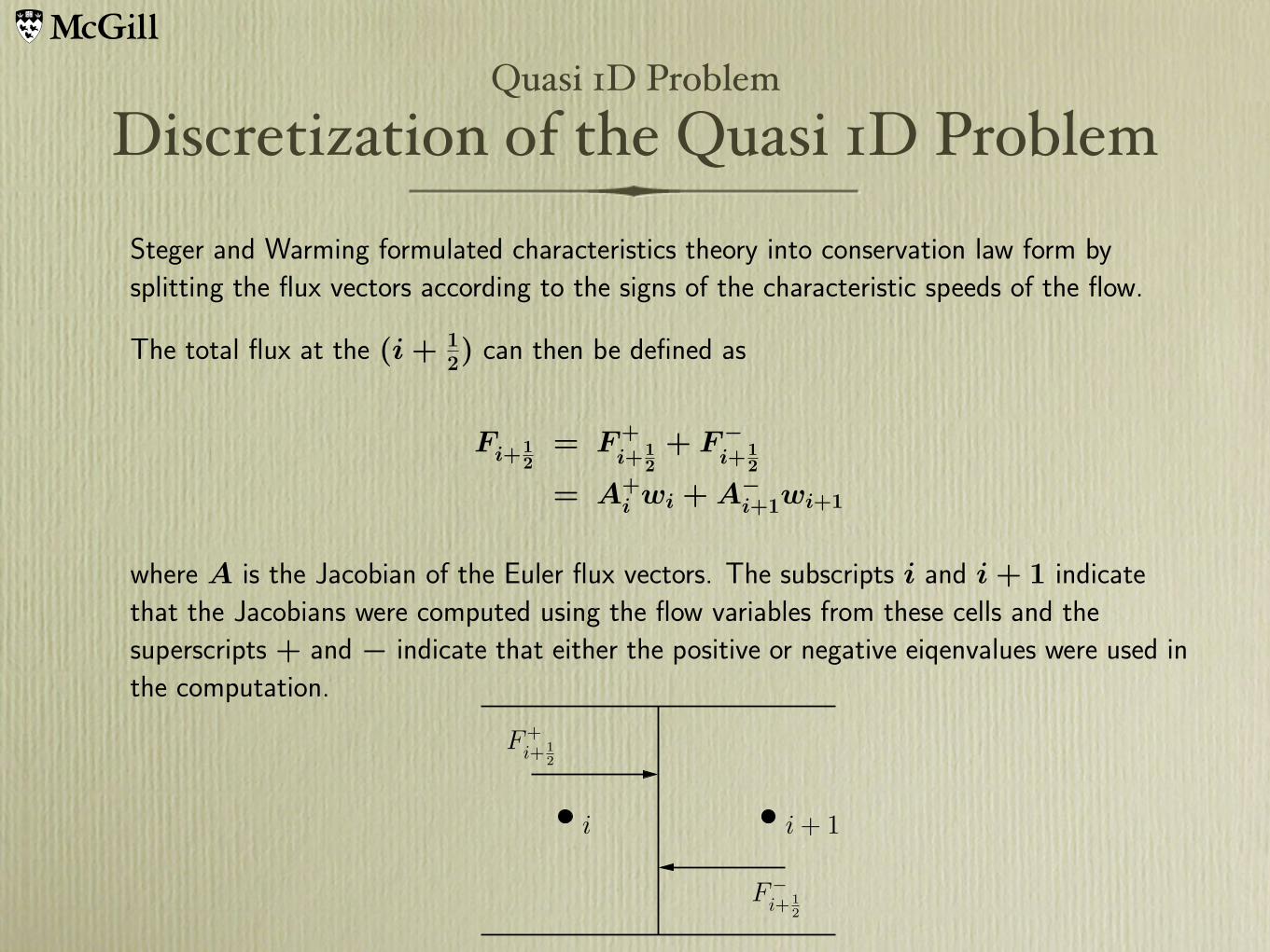
Steger and Warming formulated characteristics theory into conservation law form bysplitting the flux vectors according to the signs of the characteristic speeds of the flow.
The total flux at the (i + 12) can then be defined as
Fi+12
= F +i+1
2+ F −
i+12
= A+i wi + A−
i+1wi+1
where A is the Jacobian of the Euler flux vectors. The subscripts i and i + 1 indicatethat the Jacobians were computed using the flow variables from these cells and thesuperscripts + and − indicate that either the positive or negative eiqenvalues were used inthe computation.
Discretization of the Quasi 1D Problem
F−i+ 1
2
i + 1i
F+i+ 1
2

Quasi 1D ProblemFormulation of the Adjoint Equation
To formulate the discrete adjoint equations, we first take a variation of the residual
δR(w)i = δFi+12Si+1
2+ Fi+1
2δSi+1
2− δFi−1
2Si−1
2− Fi−1
2δSi−1
2
−
0δpi(Si+1
2− Si−1
2)
0
−
0pi(δSi+1
2− δSi−1
2)
0
Rearrange the equation to group terms that are variation of the flow field variables andvariation of the metric terms separately
δR(w)i = δFi+12Si+1
2− δFi−1
2Si−1
2−
0
δpi(Si+12
− Si−12)
0
+Fi+12δSi+1
2− Fi−1
2δSi−1
2−
0
pi(δSi+12
− δSi−12)
0

Quasi 1D ProblemFormulation of the Adjoint Equation
Next, define the variation of the fluxes across the flux boundaries
δFi+12
= A+i δwi + A−
i+1δwi+1
δFi−12
= A+i−1δwi−1 + A−
i δwi
Substitute the variation of the fluxes into the equation for the variation for the totalresidual for cell i (only terms related to the variation of the flow field variables are written)
δR(w)i =[A+
i δwi + A−i+1
]Si+1
2−
[A+
i−1δwi−1 + A−i δwi
]Si−1
2
−
0δpi(Si+1
2− Si−1
2)
0
Quasi 1D ProblemFormulation of the Adjoint Equation
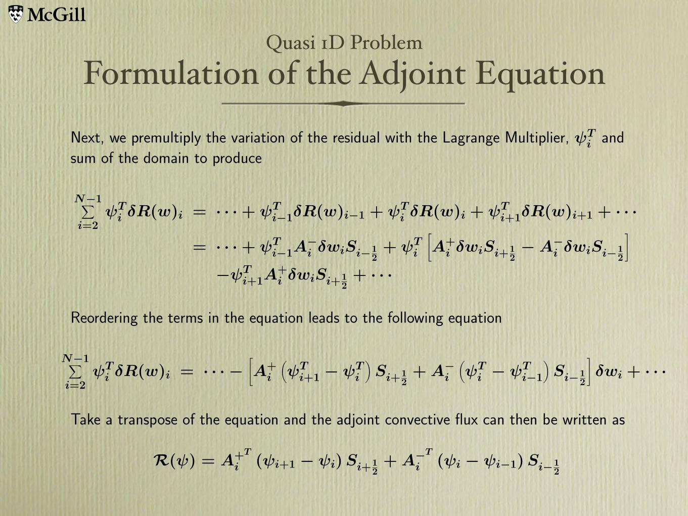
Next, we premultiply the variation of the residual with the Lagrange Multiplier, ψTi and
sum of the domain to produce
N−1∑i=2
ψTi δR(w)i = · · · + ψT
i−1δR(w)i−1 + ψTi δR(w)i + ψT
i+1δR(w)i+1 + · · ·= · · · + ψT
i−1A−i δwiSi−1
2+ ψT
i
[A+
i δwiSi+12
− A−i δwiSi−1
2
]
−ψTi+1A
+i δwiSi+1
2+ · · ·
Reordering the terms in the equation leads to the following equation
N−1∑i=2
ψTi δR(w)i = · · · −
[A+
i
(ψT
i+1 − ψTi
)Si+1
2+ A−
i
(ψT
i − ψTi−1
)Si−1
2
]δwi + · · ·
Take a transpose of the equation and the adjoint convective flux can then be written as
R(ψ) = A+T
i (ψi+1 − ψi) Si+12+ A−T
i (ψi − ψi−1) Si−12
Quasi 1D ProblemFormulation of the Adjoint Equation
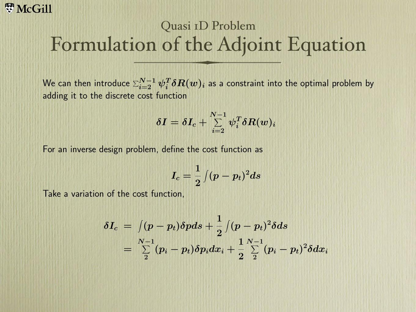
We can then introduce∑N−1
i=2 ψTi δR(w)i as a constraint into the optimal problem by
adding it to the discrete cost function
δI = δIc +N−1∑i=2
ψTi δR(w)i
For an inverse design problem, define the cost function as
Ic =1
2
∫(p − pt)
2ds
Take a variation of the cost function,
δIc =∫(p − pt)δpds +
1
2
∫(p − pt)
2δds
=N−1∑
2(pi − pt)δpidxi +
1
2
N−1∑2
(pi − pt)2δdxi

Quasi 1D ProblemFormulation of the Adjoint Equation
Sum the variation of the residual to the variation of the cost function to produce
δI =N−1∑
2(pi − pt)δpidxi +
1
2
N−1∑2
(pi − pt)2δdxi +
N−1∑i=2
ψTi δR(w)i
=N−1∑
2(pi − pt)δpidxi +
1
2
N−1∑2
(pi − pt)2δdxi
+N−1∑
2−
[A+
i
(ψT
i+1 − ψTi
)Si+1
2+ A−
i
(ψT
i − ψTi−1
)Si−1
2
]δwi
−
0ψT
i δpi(Si+12
− Si−12)
0
+ψTi Fi+1
2Si+1
2− ψT
i Fi−12Si−1
2−
0
ψTi pi(δSi+1
2− δSi−1
2)
0

Quasi 1D ProblemFormulation of the Adjoint Equation
Rearrange the equation to yield,
δI =N−1∑
2
[−
[A+
i
(ψT
i+1 − ψTi
)Si+1
2+ A−
i
(ψT
i − ψTi−1
)Si−1
2
]
+(pi − pt)δpidxi − ψTi δpi(Si+1
2− Si−1
2)
+1
2(pi − pt)
2δdxi + ψTi Fi+1
2Si+1
2− ψT
i Fi−12Si−1
2−
0
ψTi pi(δSi+1
2− δSi−1
2)
0
From here, the adjoint equation can be formed from the first line for each computationalcell
∂ψi
∂t− A+T
i (ψi+1 − ψi) Si+12
− A−T
i (ψi − ψi−1) Si−12
= 0.

Quasi 1D ProblemFormulation of the Adjoint Equation
The adjoint boundary condition can computed as
(pi − pt)dxi = −ψTi (Si+1
2− Si−1
2)
And the gradient can be calculated as
δI =1
2(pi − pt)
2δdxi + ψTi Fi+1
2Si+1
2− ψT
i Fi−12Si−1
2−
0
ψTi pi(δSi+1
2− δSi−1
2)
0

Quasi 1D ProblemTest Case
• Ni-bump geometry with a longer downstream portion of the channel.
• A channel of unit height and length, l = 8.0.
• A 1.8% thick Ni-bump of unit chord is centered about x = 6.0
• Along the upper wall, a target pressure corresponding to the presence of the same Ni-bump centered about x = 2.0 is specified, and the geometry of the complete lower surface of the channel is allowed to move so that the target pressure is obtained.
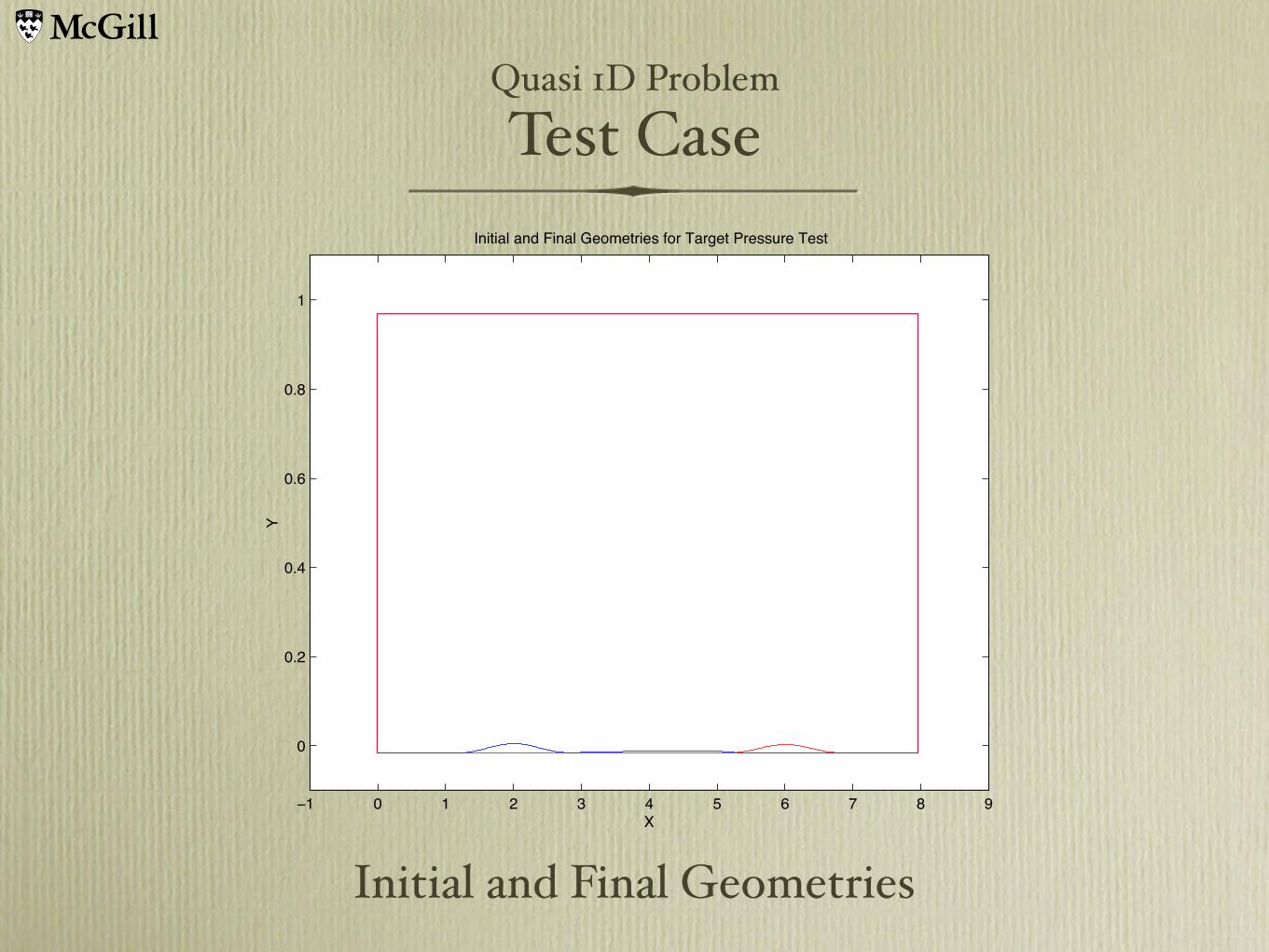
Quasi 1D ProblemTest Case
!1 0 1 2 3 4 5 6 7 8 9
0
0.2
0.4
0.6
0.8
1
X
Y
Initial and Final Geometries for Target Pressure Test
Initial and Final Geometries

Quasi 1D ProblemTest Case
!1 0 1 2 3 4 5 6 7 80.2
0.22
0.24
0.26
0.28
0.3
0.32
0.34
0.36Bottom Wall
Initial PressureTarget Pressure
!1 0 1 2 3 4 5 6 7 80.2
0.22
0.24
0.26
0.28
0.3
0.32
0.34
0.36Bottom Wall
Current PressureTarget Pressure
Pressure Distribution along the Bottom Wall Before and After Optimization

Quasi 1D ProblemTest Case
!1 0 1 2 3 4 5 6 7 80.2
0.22
0.24
0.26
0.28
0.3
0.32
0.34
0.36Top Wall
Initial PressureTarget Pressure
!1 0 1 2 3 4 5 6 7 80.2
0.22
0.24
0.26
0.28
0.3
0.32
0.34
0.36Top Wall
Current PressureTarget Pressure
Pressure Distribution along the Top Wall Before and After Optimization

Quasi 1D ProblemTest Case
!1 0 1 2 3 4 5 6 7 80.2
0.22
0.24
0.26
0.28
0.3
0.32
0.34
0.36Bottom Wall
Current PressureTarget Pressure Initial Pressure
!1 0 1 2 3 4 5 6 7 80.2
0.22
0.24
0.26
0.28
0.3
0.32
0.34
0.36Top Wall
Current PressureTarget Pressure Initial Pressure
Pressure Distribution along the Bottom and Top Walls Before and After Optimization

Quasi 1D ProblemTest Case
0.22
0.24
0.26
0.28
0.3
0.32
0.34
0 1 2 3 4 5 6 7
!3
!2
!1
0
1
2
3
4
Pressure Countours for Ni!bump Test Case
Pressure Contour