CZECH TECHNICAL UNIVERSITY IN PRAGUE

FACULTY OF NUCLEAR SCIENCES ANDPHYSICAL ENGINEERING

DIPLOMA THESIS

Quasi-Hermitian Models

Petr Siegl

Supervisor: Miloslav Znojil, DrSc., NPI AS CR RezJean-Pierre Gazeau, APC Universite Paris 7-Denis Diderot

Academic year: 2007/2008

Nazev prace: Kvazihermitovske modely

Autor: Petr SieglObor: Matematicke inzenyrstvıDruh prace: Diplomova praceVedoucı prace: Miloslav Znojil, DrSc. UJF AV CR Rez

Jean-Pierre Gazeau, APC Universite Paris 7-Denis Diderot

Abstrakt: Zkoumame vztah mezi PT -symetriı a pseudohermitovostı.Nalezneme omezeny pseudohermitovsky operator, ktery nema an-tilinearnı symetrii a take operator s antilinearnı symetriı, kterynenı pseudohermitovsky. Upozornıme na kriteria podobnostisamosdruzenemu operatoru a pripomeneme metodu pro kon-strukci metrickeho operatoru. Predstavıme tri typy modelu -retezove modely, PT -symetricke bodove interakce na prımce a su-persymetricke bodove interakce na kruznici.

Klıcova slova: PT -symmetrie, pseudohermitovost, kvazihermitovost, retezovemodely, bodove interakce, supersymetrie

Title: Quasi-Hermitian Models

Author: Petr Siegl

Abstract: We explore the relation between the PT -symmetry and thepseudo-Hermiticity, we present a bounded pseudo-Hermitian op-erator without any antilinear symmetry and also an operator withantilinear symmetry which is not pseudo-Hermitian. We recallcriteria for similarity to self-adjoint operators and the method forconstruction of metric operator. We present three types of PT -symmetric and also quasi-Hermitian models - chain models, PT -symmetric point interaction on a line and supersymmetric PT -symmetric point interactions on a loop.

Key words: PT -symmetry, pseudo-Hermiticity, quasi-Hermiticity, chain mod-els, point interactions, supersymmetry

3

Prohlasenı

Prohlasuji, ze jsem svou diplomovou praci vypracoval samostatne a pouzil jsempouze podklady (literaturu, projekty, SW atd.) uvedene v prilozenem seznamu.

Nemam zavazny duvod proti uzitı tohoto skolnıho dıla ve smyslu §60 Zakonac.121/2000 Sb., o pravu autorskem, o pravech souvisejıcıch s pravem autorskym a ozmene nekterych zakonu (autorsky zakon).

........................V Praze 1.5.2008 Petr Siegl

Acknowledgement

I would like to express my thanks to my supervisors Miloslav Znojil and Jean-PierreGazeau for their support and help. I appreciate much very valuable and inspiringdiscussions with David Krejcirık.

Contents

Introduction 5

List of Symbols 7

1 PT -symmetry and pseudo-Hermiticity 91.1 Basic properties . . . . . . . . . . . . . . . . . . . . . . . . . . . . . . 9

1.1.1 Antilinear symmetry . . . . . . . . . . . . . . . . . . . . . . . 101.1.2 Pseudo-Hermiticity . . . . . . . . . . . . . . . . . . . . . . . . 11

1.2 Equivalence relations . . . . . . . . . . . . . . . . . . . . . . . . . . . 121.2.1 Finite dimension . . . . . . . . . . . . . . . . . . . . . . . . . 131.2.2 Spectral operators of scalar type . . . . . . . . . . . . . . . . 141.2.3 Two examples . . . . . . . . . . . . . . . . . . . . . . . . . . 15

2 Quasi-Hermiticity 192.1 Basic properties . . . . . . . . . . . . . . . . . . . . . . . . . . . . . . 19

2.1.1 Similarity to self-adjoint operator . . . . . . . . . . . . . . . . 202.2 Metric operator . . . . . . . . . . . . . . . . . . . . . . . . . . . . . . 22

3 Models 283.1 Chain models . . . . . . . . . . . . . . . . . . . . . . . . . . . . . . . 28

3.1.1 The domain D for H(6) . . . . . . . . . . . . . . . . . . . . . 313.2 PT -symmetric point interaction on a line . . . . . . . . . . . . . . . 38

3.2.1 Quasi-Hermitian PT -symmetric point interactions . . . . . . 403.3 Supersymmetric PT -symmetric point interactions on a loop . . . . . 45

3.3.1 Model of the type (++) . . . . . . . . . . . . . . . . . . . . . 48

3

3.3.2 Model of the type (+−) . . . . . . . . . . . . . . . . . . . . . 513.3.3 Metric operator . . . . . . . . . . . . . . . . . . . . . . . . . . 53

4 Conclusions 55

A Selected parts of the spectral theory 57

B Spectral operators 60

C Basics of point interactions 62

D The correction of the ranges of parameters 64

References 66

4

Introduction

Quasi-Hermitian models [37] play the essential role in a so called PT -symmetricQuantum Mechanics. With regard of the fact that quasi-Hermitian operators aresimilar to the self-adjoint ones we may use them as observables. This can be doneeither by already mentioned similarity transformation or by the modification of thescalar product.

Whole PT -symmetric Quantum Mechanics itself arised from the observation thatspectrum of PT -symmetric operators, despite they are non-Hermitian, can be realand positive. This fact was revealed by Caliceti et al [12] studied by Bessis and Zinn-Justin [44] and, finally, highlighted by Bender and Boettcher [5, 6]. Mostafazadeh[26] pointed out that PT -symmetric operators are often also pseudo-Hermitian. Thisclass of operators was introduced already in 1940’s by Dirac [14] and Pauli [34].

From mathematical point of view there are still more open questions. The equiv-alence of the PT -symmetry (or more general antilinear symmetry) and the pseudo-Hermiticity is not fully solved yet, nonetheless works [28, 38, 40] bring some resultsfor special classes of operators. Discussion on the definition of quasi-Hermiticityis presented in [23], however we can find much older indeed mathematical workby Dieudonne [13]. Definition of quasi-Hermiticity presented there is more generalthen the special case usually considered within PT -symmetric Quantum Mechanics.Since quasi-Hermitian operators in sense of Diedonne may have much more extensivespectral properties (e.g. non real spectrum) we do not adopt that definition in thiswork and we retain the “standard physical” one which, in fact, is equivalent to thesimilarity to some self-adjoint operator. Criteria for similarity to self-adjoint opera-tors were found independently by several authors [41, 32, 25] and their importanceand also applicability in the context of PT -symmetry was stressed by Albeverio and

5

Kuzhel [3]. The construction of so called metric Θ is presented in [27], neverthelessonly for very special class of operators and with very formal proof without necessaryparts (convergence of the sums, domains of definition). Technically alternative pointof view, however leading to the same result, provides [23]. Examples of metric op-erator (with careful verifications of all requirements) can be found in [22] and evenfor operator with non-compact resolvent [3].

Our aim is to review and add some missing parts to general theoretical results onPT -symmetry, pseudo-Hermiticity and quasi-Hermiticity. Particularly we intend toinvestigate relation between PT -symmetry and pseudo-Hermiticity and formulatemore precisely the method of construction of metric Θ for pseudo-Hermitian op-erators with compact resolvent. The next part consists of concrete PT -symmetricmodels - chain models, PT -symmetric point interactions on a line and supersym-metric PT -symmetric point interactions on a loop.

6

List of Symbols

[·, ·] the commutator

〈·, ·〉 the scalar product

B(H) bounded linear operators acting on H

C (H) closed operators acting on H

Dom(A) the domain of A

H the separable Hilbert space

Ker(A) the kernel of A

L (H) linear operators acting on H

L (Vn) linear operators acting on Vn

X the closure of set X

Ran(A) the range of A

σ(A) the spectrum of A

σd,ess(A) the discrete and essential spectrum of A

σp,c,r(A) the point,continuous and residual spectrum of A

%(A) the resolvent set of A

ϑ Heaviside step function

7

w– lim, s– lim the limit in weak and strong operator topology

·, · the anticommutator

⊥ the orthogonal complement

A∗ the adjoint of A

AC2 absolute continuous functions with a.c. derivative and secondderivative in L2

C∞0 infinitely differentiable functions with compact support

Rλ(A) the resolvent of A at λ

Vn the linear vector space, dim Vn = n

8

Chapter 1

PT -symmetry and

pseudo-Hermiticity

1.1 Basic properties

The numerical study of Hamiltonians of the type p2 + m2x2 − (ix)N , originally forN = 3, showed that these operators may have interesting spectral properties, i.e.spectrum is real, discrete, positive. PT -symmetry was suggested to be fundamentalproperty of Hamiltonians causing reality of spectra. Traditionally, the parity P isrepresented by the linear operator acting in L2(R) space

(Pψ)(x) = ψ(−x), P2 = I, (1.1)

while the time-reversal symmetry T denotes a complex conjugation

(T ψ)(x) = ψ(x), T 2 = I, (1.2)

and PT -symmetry of Hamiltonian is understood as

PT Hψ = HPT ψ for all ψ ∈ Dom(H). (1.3)

This relation implies a symmetry of the Dom(H) as well, i.e. ψ ∈ Dom(H) if andonly if PT ψ ∈ Dom(H). The immediate consequence of the PT -symmetry foreigenvalues is that, if a complex number E is an eigenvalue of H then the complex

9

conjugate E is the eigenvalue as well

HψE = EψE ⇒ PT HψE = HPT ψE = EPT ψE . (1.4)

Moreover, if eigenfunction ψE is also PT -symmetric, i.e. PT ψE = ψE , then eigen-value E is real. This elementary proposition is often stressed and we speak aboutunbroken PT -symmetry if all eigenfunctions are PT -symmetric (and therefore alleigenvalues are real). It is obvious that the particular structure of PT operator isnot necessary for validity of these conclusions, we can generalize it in a followingway.

1.1.1 Antilinear symmetry

Definition 1.1. Let A ∈ L (H). We say that A has an antilinear symmetry if thereexists an antilinear bijective operator C and the relation

ACψ = CAψ (1.5)

holds for all ψ ∈ Dom(A).

Basic spectral properties of an operator having antilinear symmetry are given byfollowing proposition

Proposition 1.1. Let A ∈ C (H) have an antilinear symmetry C. Then λ ∈ C is inthe spectrum of A if and only if λ is in the spectrum of A. Moreover, this equivalenceis valid also for the disjoint parts of spectrum, i.e. λ ∈ σp,c,r(A)⇐⇒ λ ∈ σp,c,r(A).

Remark 1.2. We use the definition of spectrum A.1 and its point, continuous andresidual part presented in [10].

Proof. Equation (1.5) and properties of C yield the relation between resolvents

(A− λ)−1 = C−1(A− λ)−1C. (1.6)

Hence, λ ∈ %(A) ⇐⇒ λ ∈ %(A). Moreover, Ker(A − λ) = C Ker(A − λ) andRan(A− λ) = C Ran(A− λ), thus λ ∈ σp,c,r(A) ⇐⇒ λ ∈ σp,c,r(A) from the defini-tion of spectrum A.1.

Remark 1.3. An A ∈ L (H) having an antilinear symmetry is not automaticallyclosed.

10

1.1.2 Pseudo-Hermiticity

Mostafazadeh drew attention to the class of pseudo-Hermitian [26] operators becausethe studied PT -symmetric Hamiltonians possessed also this property.

Definition 1.2. Let A ∈ L (H) be densely defined. A is called weakly pseudo-Hermitian, if there exists an operator η with properties(i) η, η−1 ∈ B(H),(ii) A = η−1A∗η.If η is self-adjoint then A is called pseudo-Hermitian. If we want to specify particularη we say that A is η-(weakly)-pseudo-Hermitian.

Although pseudo-Hermiticity seems to be a stronger than weak pseudo-Hermiticity,we show that assuming the latter one only is sufficient for proving basic properties.Relation between the two properties is partly described by following theorem

Theorem 1.4 ([30]). Let A ∈ L (H) be an ηw-weakly-pseudo-Hermitian operatorand the spectrum σ(η−1

w η∗w) of η−1w η∗w does not contain the unit circle S1. Then A is

pseudo-Hermitian.

Corollary 1.5. Let A ∈ L (Vn). Then A is weakly pseudo-Hermitian if and only ifit is pseudo-Hermitian.

Unlike operators having antilinear symmetry the (weakly)-pseudo-Hermitian onesare always closed.

Lemma 1.6. Let A ∈ L (H) be a weakly pseudo-Hermitian operator. Then A isclosed.

Proof. We consider convergent sequence xn ⊂ Dom(A), xn → x for which Axnis convergent. Since η ∈ B(H), sequence yn, yn := ηxn is convergent, yn →y = ηx. Since A∗ is closed (theorem A.1), A∗yn → A∗y and y ∈ Dom(A∗). Hencex = η−1y ∈ Dom(A) and Axn = η−1A∗η xn = η−1A∗yn → η−1A∗y = Ax.

Weak pseudo-Hermiticity implies also spectral properties.

Proposition 1.7. Let A ∈ L (H) be a weakly-pseudo-Hermitian operator. Thenpoint, continuous and residual spectrum σp,c,r(A) of A and σp,c,r(A∗) of A∗ areequal.

11

Proof. Relation (ii) of the definition 1.2 yields

(A− λ)−1 = η−1(A∗ − λ)−1η. (1.7)

Since η is bounded and bijective, the equality of σp,c,r(A) and σp,c,r(A∗) holds.

1.2 Equivalence relations

Theorem A.2 shows that the equivalence λ ∈ σ(A) ⇔ λ ∈ σ(A) holds for everyweakly-pseudo-Hermitian operator A. When we return back to the spectral proper-ties of operators having antilinear symmetry and when we realize known examples ofHamiltonians which are both PT -symmetric and pseudo-Hermitian, natural ques-tions rise. Is every PT -symmetric (or operator having an antilinear symmetry)weakly-pseudo-Hermitian? Or, possesses every weakly-pseudo-Hermitian operatoran antilinear symmetry? We give some answers to these questions in the following.

In order to explain equivalence relations between PT -symmetry and pseudo-Hermiticity we present another class of operators, namely J-self-adjoint ones.

Definition 1.3 ([16]). Let A ∈ L (H) be densely defined. Let J be an antilinearisometric involution, i.e. J2 = I and 〈Jx, Jy〉 = 〈y, x〉 for all x, y ∈ H. A is calledJ-symmetric if A ⊂ JA∗J . A is called J-self-adjoint if A = JA∗J .

J-self adjoint operators were suggested by Borisov and Krejcirık [11] to be “ade-quate for a rigorous formulation of PT -symmetric problems”. One of the reasons forthis conclusion is a fact that residual spectrum of J-self adjoint operator is empty(in contrast to operators having antilinear symmetry and pseudo-Hermitian oper-ators as we shall see later). It can be easily seen that every η-pseudo-Hermitianoperator with antilinear symmetry C satisfying η2 = I, C2 = I, [η, C] = 0 and〈x, ηCy〉 = 〈y, x〉 is ηC-self-adjoint.

Lemma 1.8 ([16]). Let A be a J-self-adjoint operator. Then(i) dim(Ker(A− λ)) = dim(Ker(A∗ − λ)),(ii) σr(A) = ∅.

12

1.2.1 Finite dimension

At first, we explore relations between operators having antilinear symmetry, weakly-pseudo-Hermitian, and J-self-adjoint operators in the finite dimensional spaces.

Lemma 1.9. Every A ∈ L (Vn) is similar to the J-self-adjoint operator, i.e. thereexists invertible X ∈ L (Vn) such that XAX−1 is J-self-adjoint.

Proof. Every matrix A can be transformed to the Jordan form, i.e. A = X−1AJX,where AJ is composed of k × k Jordan blocks Jk(λ)

Jk(λ) =

λ 1

λ 1λ 1

. . .. . .

. (1.8)

Every Jordan block Jk(λ) is J-self-adjoint [18]. We provide J in the explicit form.J = PkT , where T is a complex conjugation and Pk is a k × k parity, i.e.

Pk =

11

. ..

11

. (1.9)

The above lemma is essential for the equivalence statement in finite dimensionalspaces.

Proposition 1.10. Let A ∈ L (Vn). Then A is pseudo-Hermitian if and only if itpossesses an antilinear symmetry.

Proof. Let A is pseudo-Hermitian, i.e. A = η−1A∗η. Using the lemma above

XAX−1 = AJ = JA∗JJ = J(X−1)∗A∗X∗J = J(X−1)∗ηAη−1X∗J (1.10)

we obtain CA = AC, where C := η−1X∗JX is the antilinear symmetry.

13

Let C be the antilinear symmetry of A. We find easily that

A = C−1X−1J(X−1)∗A∗X∗JXC, (1.11)

hence A is η-weakly-pseudo-Hermitian, η := X∗JXC. By corollary 1.5, A is pseudo-Hermitian.

1.2.2 Spectral operators of scalar type

Situation in Hilbert spaces with infinite dimension is of course more complicated.The problem is not solved even for bounded operators. Some results, however withnot very correct proofs, provide articles of Mostafazadeh [26, 27, 28] and more correctworks by Solombrino and Scolarici [40, 38]. All propositions of these articles requireoperators with discrete spectrum and with eigenvectors which form biorthonormalbasis. Slight generalization is presented in [38] where operators with finite Jordanblocks in spectrum may appear. We provide extension of the propositions and weprovide a new proof. We show that equivalence of weak pseudo-Hermiticity andantilinear symmetry is valid for spectral operators of scalar type. Proof for allspectral operators is not known yet (except finite Jordan blocks case [38]). SeeAppendix for the definitions and basic properties of spectral operators.

Important result for spectral operators of scalar type allows us to prove thedesired equivalence very easily.

Theorem 1.11 ([15]). Let S1, ..., Sk ∈ B(H) be commuting scalar type operatorsin H. Then there is a bounded self-adjoint operator X with a bounded everywheredefined inverse such that the operators XSiX−1, i = 1, ..., k are all normal.

Remark 1.12. We say that A ∈ L (H) is similar to B ∈ L (H) if there is aX ∈ B(H) with a bounded everywhere defined inverse and A = X−1BX. Thus,the particular case k = 1 in the theorem above states that every spectral operator ofscalar type is similar to some normal operator.

Proposition 1.13. Let S ∈ B(H) be a spectral operator of scalar type. S is weaklypseudo-Hermitian if and only if it possesses an antilinear symmetry.

Proof. S is similar to a normal operator N , S = X−1NX. Every normal operatoris J-self-adjoint [18] (proof is based on the spectral theorem for normal operators[36]). The rest of the proof is exactly the same procedure as for matrices.

14

If S is η-weakly-pseudo-Hermitian, then C := η−1X∗JX is antilinear symmetryof S. Conversely, if C is an antilinear symmetry of S then S is η-weakly-pseudo-Hermitian, where η := X∗JXC.

1.2.3 Two examples

It may seem that the weak pseudo-Hermiticity and the antilinear symmetry areequivalent properties at least for bounded operators and only some technical proofis needed. However, we present examples of bounded operators having an antilin-ear symmetry which are not weakly pseudo-Hermitian and also bounded pseudo-Hermitian operator which cannot possess any antilinear symmetry.

Example 1.1 ([35]). Let en∞n=1 be the standard orthonormal basis of H = l2(N),i.e. en(m) = δnm. Let T be an operator on H acting as

Ten := en−1, n ∈ N, e0 := 0. (1.12)

T is bounded and it possesses the antilinear symmetry T -complex conjugation. Ad-joint operator T ∗ acts as

T ∗en := en+1, n ∈ N. (1.13)

Every complex number λ with absolute value |λ| < 1 is in the point spectrum σp(T )of T , corresponding eigenvector xλ reads xλ =

∑∞n=1 λ

n−1en. Spectrum σp(T ∗) ofT ∗ is different. If we consider equation for eigenvalues

(T ∗ − λ)

( ∞∑n=1

αnen

)= 0, (1.14)

we arrive at

λα1 = 0, (1.15)

αn−1 − λαn = 0, n > 1. (1.16)

Hence, the point spectrum of T ∗ is empty. In fact, the set λ ∈ C||λ| < 1 ⊂ σr(T ∗)due to theorem A.3. Operator T is not weakly pseudo-Hermitian because the neces-sary condition is the equality of the spectrum of T and T ∗ as we have already shown(proposition 1.7).

15

Example 1.2. Let H = l2(Z) and let ei∞−∞ be the orthonormal basis, en(m) =δnm. Operator T acts as

Tei :=

λ0ei + ei+1, i ≥ 1,

0, i = 0,λ0e−1, i = −1,

λ0ei + ei+1, i < −1,

(1.17)

λ0 ∈ C, Imλ0 >12 . We find T ∗ easily from the definition of the adjoint A.3,

〈ei, T ej〉 =

λ0δi,j + δi,j+1, i, j ≥ 1,λ0δi,j + δi,j+1, i, j ≤ −1,

0, otherwise,

(1.18)

hence

T ∗ei =

λ0ei + ei−1 i > 1,

λ0e1, i = 1,0, i = 0,

λ0ei + ei−1, i ≤ −1.

(1.19)

Let P be a parity, i.e.Pei := e−i. (1.20)

We may show immediately from the definitions that T is P-pseudo-Hermitian

T = PT ∗P. (1.21)

It is obvious that λ0 ∈ σp(T ) = σp(T ∗). We show that λ0 ∈ σr(T ) = σr(T ∗). Weexpress the equation

(T − λ0)∞∑

i=−∞αiei = 0 (1.22)

and determine coefficients αi.

(T − λ0)∞∑

i=−∞αiei =

−2∑i=−∞

αi[(λ0 − λ0)ei + ei+1

]+

+α−1(λ0 − λ0)e−1 − α0λ0e0 +∞∑i=1

αiei+1, (1.23)

16

hence

αi = 0 for i ≥ 0,

αi(λ0 − λ0) + αi−1 = 0 for i < 0. (1.24)

α−1 (and then all αi) must be 0. If α−1 6= 0 then for i < −1, αi = α−1 (2 i Imλ0)−i−1 .

Since Imλ0 >12 from the definition of T ,

∞∑i=−∞

|αi|2 = +∞. (1.25)

Hence λ0 is not an eigenvalue and Ran(T − λ0) 6= H for

e1 /∈ span(ei)i 6=1 = Ran(T − λ0). (1.26)

This proves that λ0 ∈ σr(T ) and there holds also λ0 ∈ σr(T ∗) by proposition 1.7.Operator T cannot have any antilinear symmetry because the necessary condition

is that λ0 ∈ σp,c,r(T )⇔ λ0 ∈ σp,c,r(T ), by proposition 1.1.

Corollary 1.14. Weak pseudo-Hermiticity and antilinear symmetry are not equiv-alent properties even for bounded operators on H, see examples 1.1 and 1.2.

Nonetheless, it is necessary to remark that operators from previous examples arenot spectral. To justify this take into consideration

Theorem 1.15 ([15]). If the space H is separable, then the point and residual spectraof a spectral operator are countable.

Spaces l2(N) and l2(Z) are separable and we have already shown that the setλ||λ| < 1 is included in the point spectrum of the operator from the example 1.1.Similarly, the set ω =

λ ∈ C||λ− λ0| < 1

is included in the point spectrum of

the adjoint operator T ∗ from the example 1.2. Therefore, using theorem A.3, ω isincluded in the union of the point and residual spectrum of T .

For sake of completeness we discuss the relations of J-self-adjointness with anti-linear symmetry and J-self-adjointness with weak pseudo-Hermiticity.

Example 1.1 presents the operator with antilinear symmetry with non-emptyresidual spectrum, thus it cannot be even similar to J-self-adjoint operator. Con-versely, A := (i) acting in C is J-self-adjoint, where J is the complex conjugation,

17

however it cannot have any antilinear symmetry because −i is not in the spectrumof A.

Example 1.2 presents the pseudo-Hermitian operator with non-empty residualspectrum, which cannot be therefore similar to any J-self-adjoint operator. Again,operator A := (i) is J-self-adjoint, however it is not weakly pseudo-Hermitian fori /∈ σ(A∗).

18

Chapter 2

Quasi-Hermiticity

2.1 Basic properties

Quasi-Hermitian operators are very special class of pseudo-Hermitian operators.Their importance in physics was emphasized by F. G. Scholtz, H. B. Geyer and F.J. W. Hahne in [37].

Definition 2.1. Let A ∈ L (H) be densely defined. A is called quasi-Hermitian, ifthere exists an operator Θ with properties(i) Θ,Θ−1 ∈ B(H),(ii) Θ is positive,(iii) A = Θ−1A∗Θ.

In mathematics, the notion of quasi-Hermiticity appeared much earlier [13].Later, mathematically oriented discussion on the definition of quasi-Hermiticity canbe found in [23].

Remark 2.1. A more general definition of quasi-Hermiticity is presented in [13],the inverse of Θ does not need to be bounded. However, we will not use this moregeneral definition here, one of the reasons is that spectrum of such quasi-Hermitianoperator may be non real, appropriate example is presented in [13].

Remark 2.2 ([43]). For bounded operators A ∈ B(H), the existence of such Θthat 0 /∈

〈x,Θx〉

∣∣ x ∈ H, ‖x‖ = 1

and condition (iii) of the definition (2.1) issatisfied implies quasi-Hermiticity of A.

19

Reason why are quasi-Hermitian operators so important in the PT -symmetricQuantum Mechanics is that they are self-adjoint in a Hilbert spaceHΘ with modifiedscalar product

〈·, ·〉Θ := 〈·,Θ·〉 . (2.1)

The operator Θ is often called a ’metric’ or ’metric operator’ in physical litera-ture. The properties of Θ, see the definition above, guarantee that 〈·, ·〉Θ fulfills allrequirements for being scalar product and moreover

m 〈ψ,ψ〉 ≤ 〈ψ,ψ〉Θ ≤M 〈ψ,ψ〉 ∀ψ ∈ H, (2.2)

where m = inf〈ψ,Θψ〉 |ψ ∈ H, ‖ψ‖ = 1 and M = ‖Θ‖. Since Θ−1 ∈ B(H) and Θis positive, m > 0. It is possible to verify directly from the definition of the adjointoperator A.3 that quasi-Hermitian operator A is indeed self-adjoint in this scalarproduct.

2.1.1 Similarity to self-adjoint operator

Another point of view on quasi-Hermitian operators provide following proposition.

Proposition 2.3 ([3]). Let A ∈ L (H) be a quasi-Hermitian operator with metricoperator Θ. Then A is similar to the self-adjoint operator H,

A = %−1H%, (2.3)

where % =√

Θ.

The study of the problem of similarity to the self-adjoint operators may be foundin the mathematical literature [32, 41, 25]. We recall integral-resolvent criterion

Theorem 2.4 ([32]). Let A ∈ L (H). A is similar to a self-adjoint operator if andonly if

supε>0 ε

∫ ∞−∞‖(A− λI)−1ψ‖2dξ ≤M‖ψ‖2, (2.4)

supε>0 ε

∫ ∞−∞‖(A∗ − λI)−1ψ‖2dξ ≤M‖ψ‖2, (2.5)

where λ = ξ + i ε, ψ ∈ H and the integration is carried along an arbitrary straightline, parallel to the real axis, in the upper half plane.

20

This criterion is simplified when we restrict ourselves on pseudo-Hermitian op-erators.

Corollary 2.5 ([3]). Let A ∈ L (H) be a pseudo-Hermitian operator. A is similarto a self-adjoint operator if and only if the spectrum of A is real and there exists aconstant M such that

supε>0 ε

∫ ∞−∞‖(A− λI)−1ψ‖2dξ ≤M‖ψ‖2, (2.6)

where λ = ξ + i ε, ψ ∈ H and the integration is carried along an arbitrary straightline, parallel to the real axis, in the upper half plane.

For purposes of PT -symmetric Quantum Mechanics this version of the theoremmay be very useful because many known and studied PT -symmetric models arepseudo-Hermitian as well. As it is shown in [3], the latter criterion is extremelyuseful for the study of point interactions.

Another characterization of similarity of P-pseudo-Hermitian operator acting inL2(R) to self-adjoint one is given using property of C-symmetry [7, 9, 8, 3].

Definition 2.2 ([3]). Let A ∈ L (L2(R)) be a P-pseudo-Hermitian. We say thatA possesses the property of C-symmetry if there exists bounded linear operator C inL2(R) such that the following conditions are satisfied(i) AC = CA,(ii) C2 = I,(iii) for each f, g ∈ L2(R) the sesquilinear form (f, g)C := [Cf, g]P ,where [f, g]P := 〈Pf, g〉 =

∫∞−∞ f(−x)g(x)dx, determines a scalar product in L2(R)

that is equivalent to the initial one.

Proposition 2.6 ([3]). Let A ∈ L (L2(R)) be a P-pseudo-Hermitian. Then thefollowing statements are equivalent(i) A has the property of C-symmetry,(ii) A is similar to a self-adjoint operator.

It is obvious that P-pseudo-Hermitian operator acting in L2(R) that has theproperty of C-symmetry is quasi-Hermitian with the metric Θ = PC.

Authors of [3] emphasized also a necessary condition for similarity to self-adjointoperator, based on the theorem A.4.

21

Proposition 2.7. Let A ∈ L (H) be similar to a self-adjoint operator. Then thereexists real constant M such that

‖Rλ0(A)‖ ≤ M

|Imλ0|(2.7)

for all λ0 ∈ C \ R.

Proof. It follows immediately from theorem A.4 and relation between resolvents ofsimilar operators.

With regard to the simplicity of this proposition it can be very useful for provingthat an operator is not similar to self-adjoint one.

2.2 Metric operator

General resolvent criteria presented above do not provide any hint how to constructthe similarity transformation % or the metric operator Θ. Proposition 2.6 only mod-ify the problem to the construction of C-symmetry. Partial answer to this questioncan be found in [27, 31]. There is a simple criterion in finite dimensional spaces foroperators to be quasi-Hermitian.

Proposition 2.8. Let A ∈ L (Vn). Then A is quasi-Hermitian if and only if spec-trum σ(A) of A is real and A is diagonalizable. Operator Θ has form

Θ =n∑j=1

cj 〈φj , ·〉φj , (2.8)

where cj are positive real constants and φj are eigenvectors of A∗.

Proof. If A is quasi-Hermitian matrix then it is similar to Hermitian one, hence ithas real spectrum and it is diagonalizable.

If A has the real spectrum and it is diagonalizable, then

A = X−1DX, (2.9)

where D is a diagonal matrix composed of real eigenvalues. If we take adjoint of(2.9) we arrive at

XX∗A = A∗X∗X. (2.10)

Whence Θ := XX∗ is positive and it can be expressed in the form (2.8).

22

Infinite dimensional case is of course more complicated, in fact there is no gen-eral result for all quasi-Hermitian operators yet. Some results for operators withpure discrete spectrum (see definition A.7) are known. We would like to presentmore rigorous approach to the construction of the metric Θ. In order to describeeigenvectors of quasi-Hermitian operator we recall a notion of Riesz basis and a basiccriterion.

Definition 2.3 ([42]). Let en∞n=1 be an orthonormal basis in H. Then the setxn∞n=1 ⊂ H is said to be a Riesz basis if there exists a bounded invertible operatorU with bounded inverse and xn = Uen for all n ∈ N.

Theorem 2.9 ([42]). Set xn∞n=1 is a Riesz basis if and only if there exist positiveconstants m,M such that

m‖x‖2 ≤∞∑n=1

| 〈x, xn〉 |2 ≤M‖x‖2 (2.11)

for each x ∈ H.

Proposition 2.10. Let A ∈ L (H) be quasi-Hermitian operator with pure discretespectrum and metric operator Θ. Let denote ψn∞n=1, φn∞n=1 eigenvectors of Aand A∗, respectively. It is possible to normalize them in a is such way that

φn = Θψn, 〈ψi, φj〉 = δij for all i, j, n ∈ N. (2.12)

Both ψn∞n=1 and φn∞n=1 are Riesz bases and

Θ = s– limN→∞

N∑j=1

〈φj , ·〉φj . (2.13)

Proof. We denote H self-adjoint operator which is similar to A and en∞n=1 eigen-vectors of H,

H = %A%−1, % =√

Θ, Hen = λnen, ‖en‖ = 1, ∀n ∈ N. (2.14)

Since spectrum of H is pure discrete the resolvent of H is a normal compact operator,see theorem A.10. Hence normalized eigenvectors en∞n=1 form orthonormal basis.Eigenvectors ψn, φn of A, A∗ satisfy ψn = %−1en, φn = %en. Hence φn = Θψn

23

and 〈ψi, φj〉 = δij . Moreover, using functional calculus for self-adjoint operators, itfollows from requirements for Θ (definition 2.1) that % is bounded positive operatorwith bounded inverse and therefore ψn∞n=1 and φn∞n=1 are Riesz bases.

We denote ΘN :=∑N

j=1 〈φj , ·〉φj . Each x ∈ H can be uniquely expressed in theRiesz basis ψn∞n=1

x =∞∑n=1

αnψn, αn ∈ C, (2.15)

the action of ΘN then reads

ΘNx =N∑j=1

〈φj , x〉φj =N∑j=1

∞∑n=1

〈φj , αnψn〉φj =N∑n=1

αnφn. (2.16)

Relation

〈x,ΘNx〉 =N∑n=1

|αn|2 (2.17)

shows that ΘN is positive and by similar procedure, ΘN∞N=1 is an increasingsequence of positive operators. Furthermore, ΘN ≤ Θ for all N ∈ N due to

〈(Θ−ΘN )x, x〉 =∞∑

n=N+1

|αn|2. (2.18)

Hence, ΘN converges in a strong limit sense to some bounded positive operator(theorem A.11). In order to complete the proof, i.e. Θ is limit of ΘN, we showthat

Θ = w– limN→∞

ΘN . (2.19)

We take arbitrary x, y ∈ H, then

| 〈(Θ−ΘN )x, y〉 | ≤∞∑

k=N+1

|αkβk| ≤

√√√√ ∞∑k=N+1

|αk|2√√√√ ∞∑

k=N+1

|βk|2, (2.20)

where

x =∞∑n=1

αnψn, y =∞∑n=1

βnψn. (2.21)

Since %x =∑∞

n=1 αnen and %y =∑∞

n=1 βnen, the sums on the right side of (2.20)are finite and both converge to 0 for N →∞.

24

We remark that if we insert positive constants cj with property

∃ m,M > 0, m ≤ cj ≤M for all j ∈ N, (2.22)

into the sum (2.13) in the same way as in the finite dimensional case (2.8) we obtainanother metric.

It is natural to ask then, if every pseudo-Hermitian operator (or/and with anti-linear symmetry) with real and pure discrete spectrum is quasi-Hermitian. Let usassume that A is a pseudo-Hermitian operator with compact resolvent. Then, bytheorem A.7, the spectrum of A is pure discrete. Let us denote ψn, φn the eigenvec-tors of A, A∗ respectively and λn the eigenvalues. We assume that the eigenvectorsare normalized in a special way, ‖φn‖ = 1 and 〈ψn, φn〉 = 1. Let us assume furtherthat

Θ = s– limN→∞

N∑j=1

cj 〈φj , ·〉φj (2.23)

exists and it is a bounded operator for some set of positive numbers cn which satisfiesthe condition (2.22).

Particurlary, it is not possible that cn → 0 (or some subsequence ckn → 0),although this may seem to be useful for guaranteeing the convergence of (2.23).However, then 0 ∈ σ(Θ) and therefore the inverse of Θ is not bounded. If weconsider a sequence ξn = ψn/‖ψn‖ of unit vectors, then

‖Θξn‖ = ‖∞∑j=1

cj 〈φj , ξn〉φj‖ = ‖cn 〈φn, ξn〉φn‖ ≤ cn → 0. (2.24)

Without loss of generality we will assume that cn = 1 for all n ∈ N.The crucial step is to show that eigenvectors φn form a Riesz basis. First of all

it is necessary that span φ1, φ2, ... is a dense set in H, i.e. φn∞n=1 is a completesystem in H. We can show this for example by investigating Ker(Θ). If the pointspectrum σp(Θ) does not contain 0, then each x0 ∈ φ1, φ2, ...⊥ is zero vectorbecause it follows that Θx0 = 0, by inserting x0 into (2.23). Feasible analysis of thekernel of Θ using directly the sum expansion can be found e.g. in [22].

Further, the strong convergence of Θ implies the weak convergence and for allx ∈ H ⟨ ∞∑

n=1

〈φn, x〉φn, x⟩

=∞∑n=1

| 〈φn, x〉 |2 ≤ ‖Θ‖‖x‖2. (2.25)

25

Hence we obtained one of the inequalities (2.11). The second inequality exactlycorresponds with existence of a bounded inverse of Θ, i.e. whether 0 is or is not inthe continuous spectrum of Θ. This is probably the most technically difficult stepin this procedure which cannot be skipped.

Nevertheless, it is satisfied automatically for η-pseudo-Hermitian operators withantilinear symmetry C, where η and C are involutive and commuting, i.e. η2 =I, C2 = I, [η, C] = 0. Then, it is obvious that A∗ also has antilinear symmetryC and we may assume that eigenvectors φn are C invariant, it suffices to take(φn + Cφn). Furthermore, they can be normalized in such way that

〈φn, ηφm〉 = 0 for n 6= m and 〈φn, ηφn〉 = ±1 ∀n ∈ N. (2.26)

Since η is typically indefinite we cannot exclude the ’−1 case’ in the latter. Propertiesof η, C and C invariance of φn yield

〈φn, ηφm〉 = 〈φn, Cηφm〉 ∀n,m ∈ N. (2.27)

Antilinear operator Cη is surely involutive and we can assume that the set φn∞n=1

is Cη-orthonormal,〈φn, Cηφm〉 = δnm, (2.28)

it suffices to take iφk when there ’−1 case’ occurs. The essential fact then followsfrom

Theorem 2.11 ([17]). Let un∞n=1 be a complete J-orthonormal system in H, whereJ is an antilinear involution. Then following assertions are equivalent(i) for each x ∈ H

∞∑n=1

| 〈x, un〉 |2 ≤M‖x‖2, (2.29)

(ii) un∞n=1 is a Riesz basis with m = M−1.

Hence, the set φn∞n=1 with all assumptions above is a Riesz basis.It remains to verify if relation ΘAx = A∗Θx for all x ∈ Dom(A) holds. We

consider µ ∈ %(A) and rewrite the condition to following equivalent form

(A∗ − µ)−1Θx = Θ(A− µ)−1x ∀x ∈ H. (2.30)

26

Now, the expansion of arbitrary x ∈ H into the Riesz basis ψn∞n=1, relations

(A− µ)−1ψn =1

λn − µψn, (A∗ − µ)−1φn =

1λn − µ

φn (2.31)

and explicit form of Θ (2.23) are needed.We may summarize the ideas above to the proposition.

Proposition 2.12. Let A ∈ L (H) be an η-pseudo-Hermitian operator with an-tilinear symmetry C, where η and C are both involutive and commuting. Let theresolvent of A is compact for some µ ∈ C and the spectrum of A is real. If

Θ = s– limN→∞

N∑j=1

cj 〈φj , ·〉φj , (2.32)

where ‖φj‖ = 1 are eigenvectors of A∗ and cj are positive constants satisfying (2.22),is an invertible bounded operator (i.e. 0 /∈ σp(Θ)), then A is quasi-Hermitian withthe metric Θ.

Typical example of operators satisfying the assumptions of the proposition are P-pseudo-Hermitian PT -symmetric Hamiltonians with real spectrum defined on finiteinterval (a, b). We present some examples of such operators in following section.Many more examples can be found in a literature dealing with PT -symmetry. Letus stress particularly the carefully and rigorously treated model [22].

27

Chapter 3

Models

3.1 Chain models

An interesting class of finite dimensional models, so called chain-models, presentedZnojil in [48, 46, 47, 45]. It refers to N ×N tridiagonal matrices of the form

H(chain) =

1−N g1 0 0 . . . 0−g1 3−N g2 0 . . . 0

0 −g2 5−N.. .

. . ....

0 0 −g3. . . gN−2 0

......

. . .. . . N − 3 gN−1

0 0 . . . 0 −gN−1 N − 1

, (3.1)

where gn are real parameters. For sake of simplicity the parameters are assumed tobe up-down symmetric, i.e.

gN−k = gk ≥ 0, k ∈ 1, 2, ..., J, (3.2)

where N = 2J or N = 2J + 1. From the physical point of view, these tridiagonalmodels may represent a nearest neighbor-interaction perturbation of a harmonic-oscillator-like systems with shifted original equidistant eigenvalues 1, 3, 5, .... It isobvious that the finite dimensional truncated Hamiltonian H(chain) is not Hermitian

28

but PT -symmetric, where P corresponds to the N ×N matrix

P =

1−1

1. . .

. (3.3)

In spite of the fact that the technical requirements for investigation of H(chain)

increase rapidly with the dimension, several important fact have been shown in[48, 46, 47, 45].

For any dimension N there exist a J-dimensional domain D of the matrix ele-ments for which the Hamiltonian is quasi-Hermitian. The domain D is contained ina bigger one S defined by following inequalities

N3 −N2

≥ 2J−1∑n=1

g2n +

g2J , N = 2J,

2 g2J , N = 2J + 1 .

(3.4)

The set of intersections of D and ∂S is finite. These points are called extremelyexceptional points, EEP, and it is possible to write their coordinates in a closedform

g(EEP )n =

√n (N − n) , n = 1, 2, . . . , J . (3.5)

When we cross the boundary ∂D of D, some of the energies are complexified. TheEEPs are special for complexification of all energies. Thus the presented systemsmay serve as a illustration of ”quantum catastrophes”, i.e. a perturbation may causethat we leave the domain D and some energies become complex. In the domaine Dthe Hamiltonian is quasi-Hermitian, i.e. physical - we may describe the system in aHilbert space with modified scalar product (2.1).

Many numerical results, e.g. in [47], illustrates how energies may become com-plex, number of energies depends on the way out of the D. Also two dimensionaldomain D(2) for the Hamiltonian H(3) is presented,

H(3) =

−1 a 0−a 1 b

0 −b 3

P(3) =

1 0 00 −1 00 0 1

. (3.6)

29

The secular equation for H(3) reads

−E 3 + 3 E 2 +(−a2 + 1− b2

)E − 3 + 3 a2 − b2 = 0, (3.7)

and EEPs have coordinates (±√

2,±√

2). The boundary ∂D of the star-like shapedomain D may be parametrized in following way

a = a± = ±√

12

(4− 3β2 − β3), b = b± = ±√

12

(4− 3β2 + β3), (3.8)

where parameter β ∈ (−1, 1).

-1 -0.5 0 0.5 1a

-1

-0.5

0

0.5

1

b

Figure 3.1: Boundary ∂D(2)

30

3.1.1 The domain D for H(6)

We consider 6 dimensional model,

H(6) =

−5 c 0 0 0 0−c −3 b 0 0 00 −b −1 a 0 00 0 −a 1 b 00 0 0 −b 3 c

0 0 0 0 −c 5

(3.9)

and try to find the domain D. EEPs (3.5) are at (a, b, c) = (±3,±2√

2,±√

5).Secular equation for the Hamiltonian reads

χ(a, b, c, s) ≡ det(H(6) − E I

)= s3 + P1 s

2 + P2 s+ P3 = 0 , s = E2, (3.10)

where

P1 = a2 + 2b2 + 2c2 − 35,

P2 = 259− 34a2 − 44b2 + b4 + 28c2 + 2a2c2 + 2b2c2 + c4, (3.11)

P3 = −225 + 225a2 − 150b2 − 25b4 − 30c2 + 30a2c2 − 10b2c2 − c4 + a2c4.

Elementary analysis of the roots of (3.10) (s must be non-negative for E ∈ R) yieldsthat the domain D(3) is contained in the area determined by conditions P1,2,3 ≥ 0,see figure 3.2. In order to fully determine the domain D we analyse the qualitativemeaning of the parameter a, b, c, i.e. their impact on properties of the characteristicpolynomial χ. H(6) is obviously Hermitian for a = 0, b = 0, c = 0. E = s2, hencethe complexification of energies E may occur for several reason:(i) one or more roots s are negative,(ii) two roots s are non-real, (complex conjugated to each other).The second possibility may happen if the local minimum of χ is below zero (or thelocal maximum is above zero). Figure 3.3 illustrates, how the position of roots andlocal extremes is modified with respect to change of parameters a, b, c. Thus, theboundary of the domain D is defined by surface S1 corresponding to the conditionP3 = s1.s2.s3 = 0, where we denoted s1,2,3 the roots of χ, and surfaces S2,3 deter-mined by the condition that the local extremes of χ are zero. Local extremes χ are

31

P1

-5-2.5

02.5

5

-4-2

02

4

-4

-2

0

2

4

-5-2.5

02.5

5

-4-2

02

4

(a) P1 = 0

P2

-2

0

2

-2

0

2

-2

-1

0

1

2

-2

0

2

-2

0

2

(b) P2 = 0

P3

-5

0

5

-5

-2.5

02.5

5

-5

-2.5

0

2.5

5

-5

0

5

-5

-2.5

02.5

5

(c) P3 = 0

Figure 3.2: Areas determined by Pi = 0

situated at points x1,2

x1,2 =13

(35− a2 − 2b2 − 2c2 ±

±√

448 + 32a2 + a4 − 8b2 + 4a2b2 + b4 − 224c2 − 2a2c2 + 2b2c2 + c4). (3.12)

Hence conditions χ(a, b, c, x1,2) = 0 determine the surfaces S2,3, see figure 3.5, wherethe red points are EEPs. The intersection of the surfaces illustrates figure 3.4

Answer to the question how and how many energies are complexified provide fig-ures 3.6,3.7, where the colors of the graphs of χ and areas correspond (white=black).Two energies are complexified in the orange area - there is one negative s root. Fourenergies are complexified in the yellow area - there are two negative s roots, andin the white area - there are two complex conjugated s roots. Finally, all six en-ergies are complexified in the green area - there are one negative and two complexconjugated s roots.

32

-5 5 10 15 20 25

-2500

-2000

-1500

-1000

-500

0, 0, 0

a, b, c

(a) a, b, c = 0

-10 -5 5 10 15 20 25

-3000

-2000

-1000

2.0,0.1,0.1

1.3,0.1,0.1

0.1,0.1,0.1

a, b, c

(b) a-dependence

-10 -5 5 10 15 20 25

-5000

-4000

-3000

-2000

-1000

0.1,2.0,0.1

0.1,1.3,0.1

0.1,0.1,0.1

a, b, c

(c) b-dependence

-10 -5 5 10 15 20 25

-3000

-2000

-1000

1000

2000

3000

0.1,0.1,2.0

0.1,0.1,1.3

0.1,0.1,0.1

a, b, c

(d) c-dependence

Figure 3.3: Characteristic polynomial χ

33

-2

0

2a

-2

0

2b

-2

-1

0

1

2

c

-2

0

2a

-2

0

2b

Figure 3.4: The intersection of S1,2,3

34

-2

0

2

-2

0

2

-2

-1

0

1

2

-2

0

2

-2

0

2

(a) Surface S1

-2

0

2

-2

0

2

-2

-1

0

1

2

-2

0

2

-2

0

2

(b) Surface S2

-2

0

2

-2

0

2

-2

-1

0

1

2

-2

0

2

-2

0

2

(c) Surface S3

-2

0

2

-2

0

2

-2

-1

0

1

2

-2

0

2

-2

0

2

(d) The domainD with EEPs

Figure 3.5: Surfaces S1,2,3 and the domain D with EEPs.

35

-30 -20 -10 10 20 30

-10000

-5000

5000

3.5, 3.5, 0.1

0.1, 1.2, 0.1

0.1, 0.1, 1.2

3.0, 0.1, 1.2

3.0, 0.1, 0.1

0.1, 0.1, 0.1

a, b, c

Figure 3.6: Characteristic polynomial χ

36

Figure 3.7: The domain D and areas of complexification

37

3.2 PT -symmetric point interaction on a line

Typical one dimensional PT -symmetric physical systems are Hamiltonians actingin L2(R) of the form

H = − d2

dx2+ V (x), (3.13)

where potential V is a complex function satisfying

V (−x) = V (x). (3.14)

Although PT -symmetry does not guarantee the reality of spectrum, many suchsystems were discovered and intensively studied. It is natural that systems withvarious types of potential may be very complicated and only little of them are exactlysolvable. PT -symmetry, in sense of non-self-adjointness, brings another difficulties.In order to obtain some suitable solvable models we use point interactions. Thepoint interaction should be understood as any interaction which does not affect thefunction with the support separated from the point where interaction acts. Theory ofstandard Hermitian point interactions, which is based on the self-adjoint extensionsof symmetric operators, is well described in several monographs, we mention one ofthem [2]. Some elementary facts about self-adjoint extensions of symmetric operatorsand point interactions in one dimension can be found in Appendix. The methodsfor self-adjoint operators are not applicable for PT -symmetric systems and they hasto be modified.

The most important initial work on PT -symmetric point interactions is done in[1]. Another papers presents concrete systems on a line or finite interval [29, 49]. Atfirst, we summarize the main principles and results. Then, we extend the results of[3] concerning the relation between systems with one point interaction on a line andquasi-Hermitian operators. Next section is devoted to supersymmetrical systemswith two PT -symmetric point interactions on a finite interval.

We consider one point interaction at the origin. More technically speaking, wetake a second derivative operator L0 = −(d2/dx2) with the domain

Dom(L0) = C∞0 (R \ 0) (3.15)

as a starting point. The adjoint L∗0 is again the second derivative L∗0 = −(d2/dx2),

38

however with the domain

Dom(L∗0) = AC2(R \ 0). (3.16)

We use the notation of [10], ψ ∈ AC2(Ω) if ψ,ψ′ are absolutely continuous at Ω andψ′′ ∈ L2. Any PT -symmetric point interaction is represented by PT -symmetricextension of L0 (or restriction of L∗0). Thus we describe the point interactions byboundary conditions.

Theorem 3.1 ([1]). The family of PT -symmetric second derivative operators withpoint interactions at the origin coincides with the set of restrictions of the secondderivative operator Lmax = − d2

dx2 , defined on AC2(R \ 0), to the domain of func-tions satisfying the boundary conditions at the origin of one of the following twotypes

1. (ψ(0+)ψ′(0+)

)= B

(ψ(0−)ψ′(0−)

)(3.17)

with the matrix B equal to

B = eiθ

( √1 + bceiφ b

c√

1 + bce−iφ

)(3.18)

with the real parameters b ≥ 0, c ≥ −1/b, θ, φ ∈ [0, 2π)

2.

h0ψ′(0+) = h1e

iθψ(0+) (3.19)

h0ψ′(0−) = −h1e

−iθψ(0−) (3.20)

with the real phase parameter θ ∈ [0, 2π) and with the parameter h = (h0, h1)taken from the (real) projective space P1.

The symbols 0± have usual meaning of limits, ψ(0±) = limx→0± ψ(x). Boundaryconditions of the first type are called connected, conditions of the second type arecalled separated. Further we deal with connected boundary conditions only becausethe separated case can be decomposed to two separated systems on a half-line.

39

Although the original statement of [1] includes that the restricted operators areboth PT -symmetric and P-pseudo-Hermitian for the entire range of parametersb, c, θ, φ, we show that P-pseudo-Hermiticity is ensured only for θ = 0 (other rangesof parameters are preserved), see Appendix for the details. Nevertheless, the oper-ators for θ 6= 0 and θ = 0 are unitary equivalent [1].

Spectrum of Hamiltonians with PT -symmetric point interactions is described byfollowing

Theorem 3.2 ([1]). The spectrum of any PT -symmetric second derivative operatorwith point interactions at the origin consists of the branch [0,∞) of the absolutelycontinuous spectrum and at most two (counting multiplicity) eigenvalues, which arereal negative or are complex conjugated to each other.

Proposition 3.3 ([1]). The spectrum of the PT -symmetric second derivative op-erator with connected point interaction at the origin is pure real if and only if theparameters appearing in theorem 3.1 satisfy in addition at least one of the followingconditions(i) bc sin2 φ ≤ cos2 φ,

(ii) bc sin2 φ ≥ cos2 φ and cosφ ≥ 0.

3.2.1 Quasi-Hermitian PT -symmetric point interactions

Our aim is to classify the Hamiltonians with one PT -symmetric point interactionwhich have real spectrum according to their similarity to self-adjoint operator, i.e.quasi-Hermiticity. Analysis of a such type has been already done in [3] for specialsubclass of Hamiltonians with one PT -symmetric point interaction correspondingto the potential composed of δ and δ′ functions

V = a 〈δ, ·〉 δ + b⟨δ′, ·⟩δ + c 〈δ, ·〉 δ′ + d

⟨δ′, ·⟩δ′, (3.21)

where a, d ∈ R and c = −b. The results show that the reality of spectrum itself doesnot guarantee quasi-Hermiticity.

Technically, we use the resolvent criterion, theorem 2.5, and necessary conditionfor similarity to self-adjoint operator, proposition 2.7. To be able to use these criteriawe calculate resolvent Rλ(H) of the Hamiltonian H = −(d2/dx2) with the domain

Dom(H) =ψ ∈ AC2(R \ 0)

∣∣ψ satisfies (3.17, 3.18). (3.22)

40

We denote k the square root of λ and to obtain unique k pro every λ ∈ C werequire Im k ≥ 0. We introduce two functions e+ and e−

e+(x) = ϑ(x)eikx, e−(x) = ϑ(−x)e−ikx, (3.23)

where ϑ is a Heaviside step function. Then resolvent Rλ(H) can be written forarbitrary f ∈ L2(R) in the form

g(x) ≡ Rλ(H)f(x) = (Rλ(H0)f)(x) + C+(f)e+(x) + C−(f)e−(x), (3.24)

whereRλ(H0)f(x) =

i2k

∫ ∞−∞

eik|x−y|f(y)dy (3.25)

is well-known formula for self-adjoint free particle Hamiltonian and C± are param-eters to be calculated.

g(0+) = i2k (f− + f+) + C+(f), g′(0+) = −1

2(f− − f+) + ikC+(f),g(0−) = i

2k (f− + f+) + C−(f), g′(0−) = −12(f− − f+)− ikC−(f),

(3.26)

wheref± =

∫R±

e±ikyf(y)dy. (3.27)

Function g = Rλ(H)f must satisfy the boundary conditions (3.18) thus(eiθ(ibk −

√1 + bc eiφ) 1

eiθ(ik√

1 + bc e−iφ − c) ik

).

(C−

C+

)=(

12k

(k(f− − f+) +

√1 + bc ei(θ−φ)k(−f− + f+) + iceiθ(f− + f+)

)i2

((√1 + bc ei(θ+φ) − 1

)(f− + f+) + ibeiθk(f− − f+)

) ). (3.28)

This system of linear equations is solvable if and only if the determinant of thematrix is nonzero

eiθ(bk2 + 2ki

√1 + bc cosφ− c

)6= 0. (3.29)

Then the solutions can be written as

C−(f) =−1

2kp(k)

[2k(√

1 + bc f+ cosφ− f+ cosφ)

+ ic(f− + f+) +

ibk2(f− − f+) + 2ik(f+ sinφ+√

1 + bc f− sinφ)],

C+(f) =ie−iφ

2kp(k)

[k(eiφ(bk(f− − f+) + 2

√1 + bc (if− cosφ+ f+ sinφ)) +

2f−(

sin(θ + φ)− i cos(θ + φ)))− ceiφ(f− + f+)

], (3.30)

41

wherep(k) = bk2 + 2ki

√1 + bc cosφ− c. (3.31)

Proposition 3.4. Let H ∈ L (L2(R)) be a Hamiltonian corresponding to onePT -symmetric point interaction at the origin (3.22). Let parameters b, c, φ sat-isfy bc sin2 φ ≤ cos2 φ (i.e. spectrum of H is real, proposition 3.3). If in additionone of the following conditions for parameters is satisfied

(i) c > 0, cosφ < 0, b ≥ 0,(ii) c = 0, cosφ ≤ 0, b > 0,(iii) c < 0, cosφ ≥ 0, b > 0,(iv) c < 0, cosφ > 0, b = 0,

then H is not similar to any self-adjoint operator.

Proof. If H is similar to a self-adjoint operator then the inequality from the propo-sition 2.7 holds for every g ∈ L2(R). Further, Rλ(H0) (3.25) is resolvent of theself-adjoint operator, thus for every λ ∈ C \ R

‖ (Rλ(H)−Rλ(H0)) g‖2 ≤ M

(Imλ)2‖g‖2, (3.32)

where M is a positive constant independent of λ and g, is valid for each g ∈ L2(R),particularly for

g0(x) = ϑ(x)e−ikx, (3.33)

where ϑ is a Heaviside step function, and k2 = λ and Im k > 0. We calculate thenorms

‖g0‖2 =1

2Im k, ‖e±‖2 =

12Im k

, (3.34)

and together with relations (3.30) and identities (Imλ)2 = 4(Im k)2(Re k)2 we receivecondition (3.32) in the explicit form(∣∣∣∣ i

2+

ic+ k√

1 + bc e−iφ

p(k)

∣∣∣∣2 +∣∣∣∣− i

2+ke−iθ

p(k)

∣∣∣∣2)

(Re k)2

|k|2≤M, (3.35)

where p(k) has been already defined (3.31). If we take into account that roots ofp(k) (for non degenerate case b 6= 0) read

k1,2 = − ib

cosφ(√

1 + bc±√

cos2 φ− bc sin2 φ

), (3.36)

42

we may easily prove that if parameters b, c, φ satisfy at least one of the conditionsthen left hand side of (3.35) tends to infinity in the neighborhood of k1,2.

We intend to show the similarity to a self-adjoint operator for class of PT -symmetric point interactions using criterion of the theorem 2.5. To make the proofmore technically feasible we at first modify relations (3.30) for functions fr,l(x) :=ϑ(±x)f(x)

C−(fl) =(

i2

+ic+ k

√1 + bc eiφ

p(k)

)fl−k,

C−(fr) =(− i

2+ke−iθ

p(k)

)fr+k,

C+(fl) =(− i

2+keiθ

p(k)

)fl−k,

C+(fr) =(

i2

+ic+ k

√1 + bc ei−φ

p(k)

)fr+k. (3.37)

Proposition 3.5. Let H ∈ L (L2(R)) be a Hamiltonian corresponding to one PT -symmetric point interaction at the origin (3.22). Let parameters b, c, φ satisfy(I) bc sin2 φ ≥ cos2 φ and cosφ ≥ 0,or(II) bc sin2 φ ≤ cos2 φ

with at least one of the following conditions in addition(i) c > 0, cosφ > 0, b > 0,(ii) c > 0, cosφ = 0, b = 0,(iii) c = 0, cosφ > 0, b 6= 0,(iv) c = 0, cosφ 6= 0, b = 0,(v) c < 0, cosφ = 0, b = 0,(vi) c < 0, cosφ < 0,

then H is similar to a self-adjoint operator.

Proof. Taking into account theorem 2.5, the existence of a constant M such that forall g ∈ L2(R)

supε>0 ε

∫ ∞−∞‖ (Rλ(H)−Rλ(H0)) g‖2dξ ≤M‖g‖2, (3.38)

43

where λ = ξ + i ε and the resolvents Rλ(H), Rλ(H0) are defined above, alreadyguarantee the similarity to self-adjoint operator. At first, we consider function gr,where gr,l(x) := ϑ(±x)g(x). Using relations (3.34, 3.37) and λ = k2, Im k > 0 wearrive at

‖ (Rλ(H)−Rλ(H0)) gr‖2 =

=

(∣∣∣∣ i2

+ic+ k

√1 + bc e−iφ

p(k)

∣∣∣∣2 +∣∣∣∣− i

2+ke−iθ

p(k)

∣∣∣∣2)

︸ ︷︷ ︸Mr(k)

|gr+|2

2|k|2Im k, (3.39)

where gr+ is defined by (3.27) and p(k) by (3.31). Since we assumed (I), or (II) withat least one of the (i)-(vi), roots of p(k) are located in the lower complex half-plane(Im k < 0). Thus Mr(k) < Mr for all k ∈ C, Im k > 0. (Little bit more delicate casec = 0 when one root is equal zero can be resolved by elementary analysis of Mr(k),the estimate is valid as well.) Next we estimate the resting parts, using changingof integration variables, fact that gr+ is Fourier transformation of gr and Carlesonembedding theorem [21, 3],∫ ∞

−∞

ε|gr+(k)|2

|k|2Im kdξ = 4

∫ ∞0|gr+(k)|2dRe k ≤ π

2M‖gr‖2, (3.40)

where M is a constant independent of k and gr. All together we have

ε

∫ ∞−∞‖(Rλ(H)−1 −Rλ(H0)

)gr‖2dξ <

π

2MrM‖gr‖2. (3.41)

We can use the similar procedure to gl and we obtain almost the same result (con-stants can be different). Hence H is similar to self-adjoint operator.

Using the theorem 2.5 and the same technique we may also classify all systemswith one point interaction (not necessarily PT -symmetric) on a line with real spec-trum. It is possible to show that example of a complex delta interaction [29] is (intherein considered setting of the parameter) similar to self-adjoint operator. Thisresult, in fact, justifies the effort to construct the metric for this system [29].

44

3.3 Supersymmetric PT -symmetric point interactions

on a loop

We consider a system on the finite interval (−l, l) and two point interactions, atx = 0 and x = ±l (i.e. interaction at origin and between the two end points).PT -symmetric point interaction are described by boundary conditions theorem 3.1,however, in order to show connection with self-adjoint case [33] we rewrite theseconditions in the following form, using the same parameters b, c, θ, φ

(C − I)Ψ(a) + (C + I)Ψ′(a) = 0, (3.42)

where

Ψ(a) =

(ψ(a+)ψ(a−)

), Ψ′(a) =

(ψ′(a+)−ψ′(a−)

), (3.43)

C =

(b−c)eiφ+√

1+bc(e2iφ−1)

(b+c)eiφ+√

1+bc(e2iφ+1)2e(θ+φ)

(b+c)eiφ+√

1+bc(e2iφ+1)

2e(−θ+φ)

(b+c)eiφ+√

1+bc(e2iφ+1)

(b−c)eiφ−√

1+bc(e2iφ−1)

(b+c)eiφ+√

1+bc(e2iφ+1)

. (3.44)

Our aim is to find PT -symmetric systems on a loop (−l, l) with two point interac-tions (at 0 and l) which are supersymmetric. Various supersymmetric PT -symmetricsystems were intensively studied, e.g. [24, 4]. We would like to take advantage ofusual simplicity (exact solvability in terms of elementary functions) of Hamiltonianswith point interactions and moreover its special structure (SUSY) to find explicitlythe spectra and metric Θ operators for these systems.

In order to obtain supersymmetric system with supercharges Q1,2 ∝ ddx ,

Qa, Qb = Hδab, (3.45)

we have to restrict boundary conditions (3.42)-(3.44). We expect that we receiveboundary conditions which connect values of functions and values of derivativesseparately as well as in a self-adjoint case [33].

We recall briefly the procedure of finding suitable boundary conditions compat-ible with supersymmetry presented in [33] and we modify it to the PT -symmetriccase.

If ϕ is an eigenfunction of H then Qϕ is also eigenfunction of H correspondingto the same eigenvalue (or Qϕ = 0). Since it is not guaranteed for general boundary

45

conditions that Qϕ satisfies (3.42) although ϕ does, supercharges cannot be onlyderivatives multiplied by a scalar. We take an eigenfunction ϕ of H

Hϕ = Eϕ (3.46)

and denote χ ≡ Qϕ. Since the supercharge is proportional to the derivative, bound-ary values of χ are related to those of ϕ′

Ψχ(a) ≡

(χ(a+)χ(a−)

)= M

(ϕ′(a+)−ϕ′(a−)

), (3.47)

where M is an invertible matrix. ϕ is an eigenfunction of H, hence ϕ′′ is proportionalto ϕ and

Ψ′χ(a) ≡

(χ′(a+)−χ′(a−)

)= EM

(ϕ(a+)ϕ(a−)

), (3.48)

where M is an invertible matrix again. When we combine (3.42),(3.47),(3.48) wearrive at

(C − I)M−1Ψ′χ(0) + E(C + I)M−1Ψχ(0) = 0. (3.49)

Boundary conditions have to be energy independent and Ψχ, Ψ′χ are not zero vectorssimultaneously. Therefore (C ± I) must be singular matrices, i.e. eigenvalues of Care ±1. This constraint restricts general form of C to two possibilities

C± = ±

(i tanφ eiθ

cosφe−iθ

cosφ −i tanφ

), (3.50)

i.e. parameters b, c are equal to zero however the range of θ, φ is preserved.After reparametrization of C± elements using new both ~β and ~b parameters

β1 = b1 = − cos θcosφ

, β2 = b2 =sin θcosφ

, β3 = ib3 = −i tanφ, (3.51)

(~β) 2 = b21 + b22 − b23 = 1, β1,2 ∈ R, β3 ∈ iR, b1,2,3 ∈ R, (3.52)

we arrive atC± = exp

(iπ

2(I ± ~β.~σ)

), (3.53)

where ~σ are the Pauli matrices.We use parameters ~β in order to write following expressions in more elegant way

and to show connection with the self-adjoint case, where parameters real ~α are used,

46

see (3.54, 3.55). However, we move to real parameters ~b in the following to avoidthe tricky structure of ~β, β3 is not real.

We summarize results for self-adjoint case in following and adapt them to thePT -symmetric case. Fortunately, the transition from the self-adjoint case turnedout to be very easy, in fact a shift ~α 7→ ~β is needed only. The direct connection canbe found in the relation (3.53) because it is a slight generalization of the standardone (3.56).

Boundary conditions for the self-adjoint case are described by unitary matrix Uand real parameter L0 in equation (C.4) where Ψ, Ψ′ are correspond to (3.43). Wemay use an exponential form of unitary matrix

U ≡ Ug(θ+, θ−) = exp

iθ+P+g + iθ−P−g

, (3.54)

where P±g are orthogonal projectors

P±g =12

(I ± g), g = ~α.~σ, ~α ∈ R3, (~α)2 = 1,

(P±g )2 = P±g = (P±g )∗, P±g P∓g = 0, P+

g + P−g = I. (3.55)

Supersymmetry restricts (proof in [33]) these general conditions to

Ug(π, 0) = exp

iπ

2(I ± ~α.~σ)

. (3.56)

Although we cannot use the exponential form for the general matrix C (3.44), bothmatrices Ug(π, 0) and C± with restricted parameters may be written in the exponen-tial form (3.53), (3.56). We note that the only difference between Ug(π, 0) and C±

is the structure of ~α and ~β. This fact allows us to obtain supercharges, eigenvaluesand eigenfunctions of Hamiltonian very easily from the self-adjoint case.

In order to express boundary conditions in more convenient way we use operatorsP,Q,R,

(Pψ)(x) = ψ(−x), (Rψ)(x) = (ϑ(x)− ϑ(−x))ψ(x), Q = −iRP, (3.57)

where ϑ is a Heaviside step function. The operators are labeled in following way

P1 ≡ P, P2 ≡ Q, P3 ≡ R. (3.58)

47

The set of these operators forms an algebra of Pauli matrices, i.e.

[Pl,Pm] = 2iεlmnPn,

Pl,Pm = 2δlmI. (3.59)

Next, operator G associated to g = ~β.~σ is introduced

G = ~β. ~P, (3.60)

obeying G2 = I, G∗ 6= G, [G,PT ] = 0. (In the self-adjoint case is ~β replaced by ~α andG is self-adjoint.) It allows us to decompose any function ψ into two eigenfunctionsof G

ψ± =12

(I ± G)ψ, ψ = ψ+ + ψ−, Gψ± = ±ψ±. (3.61)

Boundary conditions at x = a corresponding to C± are now expressed in theform

type + : ψ+(a+) = ψ′−(a−) = 0, type − : ψ′+(a+) = ψ−(a−) = 0. (3.62)

Hence we study two types of models: (++) and (+−). (++) denotes the interactionof the type + at x = 0 and of the type − at x = l (at x = l boundary conditionsconnect x = −l and x = l). The other combinations provide equivalent models.

3.3.1 Model of the type (++)

We work in the Hilbert space L2(−l, l). The domain of definition of our HamiltonianH1 ≡ H++ = − d2

dx2 consists of functions ψ ∈ AC2(Ω), where Ω = (−l, 0) ∪ (0, l),which obey boundary conditions (++) at x = 0 and x = ±l.

Dom(H1) : ψ ∈ AC2(Ω),(b1 + ib2)ψ(0+) + (1− ib3)ψ(0−) = 0,(b1 + ib2)ψ′(0+) + (1 + ib3)ψ′(0−) = 0,(b1 + ib2)ψ(l) + (1− ib3)ψ(−l) = 0,(b1 + ib2)ψ′(l) + (1 + ib3)ψ′(−l) = 0,b1,2,3 ∈ R, b21 + b22 − b23 = 1,

(3.63)

where b1,2,3 ∈ R and b21 + b22 − b23 = 1. Since the fractions (1 ± ib3)/(b1 + ib2) haveabsolute values equal to one, boundary conditions may be rewritten as

ψ(0+) = eiτ1ψ(0−), ψ′(0+) = eiτ2ψ′(0−), τ1,2 ∈ R, (3.64)

48

for x = ±l similarly. Parameters τ1,2 are different if b3 6= 0, the case b3 = 0corresponds to the self-adjoint setting.

It is not difficult to find the adjoint operator H∗1 directly from the definition ofadjoint operator A.3, i.e. using standard technique, integration by parts etc.

Dom(H∗1 ) : ψ ∈ AC2(Ω),(b1 + ib2)ψ(0+) + (1 + ib3)ψ(0−) = 0,(b1 + ib2)ψ′(0+) + (1− ib3)ψ′(0−) = 0,(b1 + ib2)ψ(l) + (1 + ib3)ψ(−l) = 0,(b1 + ib2)ψ′(l) + (1− ib3)ψ′(−l) = 0,b1,2,3 ∈ R, b21 + b22 − b23 = 1.

(3.65)

Since H1 is equal to H∗−b3 (we change a sign of b3 in (3.63) and take the adjoint)it is closed. We remark that H1 is P-pseudo-Hermitian only for b2 = 0. It is clearfrom the theorem A.8 that H1 is operator with compact resolvent.

Eigenvalues of H1 are the same as in self-adjoint case [33], eigenfunctions differonly in the substitution ~α 7→ ~b, i.e.

En =(nπl

)2,

ψn+(x) = Cn

(ϑ(x)− ϑ(−x)

b1 + ib21 + ib3

)sin

nπ

lx,

ψn−(x) = Cn

(ϑ(x)− ϑ(−x)

b1 + ib21− ib3

)cos

nπ

lx, n ∈ N0, (3.66)

where ϑ(x) is a Heaviside step function and Cn are normalization constants. Eigen-functions of Hamiltonian ψn± are eigenfunctions of operator G (3.60) as well, corre-sponding to eigenvalues ±1 (the generalization of the proof from the self-adjoint caseis straightforward). Figures 3.8, 3.9 illustrate eigenfunctions ψ5±, point interactionsat the origin and end points rotate wavefunction in the complex plane.

Energy levels are doubly degenerate except the lowest one as we expected for thesupersymmetric system. Supercharges Q1,2 may be obtained from the self-adjointcase [33] easily again, by substitution ~α 7→ ~β

Q1,2 = i√

22G1,2P3

d

dx, (3.67)

whereG1,2 = ~γ1,2. ~P, (~γ1,2)2 = 1 and ~γ1,2.~β = ~γ1.~γ2 = 0. (3.68)

49

-Π

0

Π

x

Im

Re

Figure 3.8: Eigenfunction ψ5+, ~b = (10.000, 5.600, 11.417), l = π

-Π

0

Π

x Im

Re-Π

0x

Figure 3.9: Eigenfunction ψ5−, ~b = (10.000, 5.600, 11.417), l = π

Eigenfunctions of Hamiltonian have very simple form and this fact allows us toconstruct metric Θ operator using (2.23).

We denote φn± eigenfunctions of H∗ and normalize them in a special way

φn+(x) =

√2l

(ϑ(x)− ϑ(−x)

b1 + ib21− ib3

)sin

nπ

lx,

φ0−(x) =1√l

(ϑ(x)− ϑ(−x)

b1 + ib21 + ib3

),

φn−(x) =

√2l

(ϑ(x)− ϑ(−x)

b1 + ib21 + ib3

)cos

nπ

lx. (3.69)

50

Sets e±n ∞n=1, f±n ∞n=0

e±n (x) =

√2lϑ(±x) sin

nπ

lx,

f±0 (x) =1√lϑ(±x), f±n (x) =

√2lϑ(±x) cos

nπ

lx, (3.70)

form orthonormal bases of L2(−l, 0) and L2(0, l). We express φn± in terms of e±n , f±n

and calculate

〈φn+, ψ〉φn+ =⟨e+n , ψ

⟩e+n +

⟨e−n , ψ

⟩e−n +

b1 + ib21− ib3

⟨e−n ,Pψ

⟩e−n +

+b1 − ib21 + ib3

⟨e+n ,Pψ

⟩e+n ,

〈φn−, ψ〉φn− =⟨e+n , ψ

⟩f+n +

⟨f−n , ψ

⟩f−n −

b1 + ib21 + ib3

⟨f−n ,Pψ

⟩f−n −

−b1 − ib21− ib3

⟨f+n ,Pψ

⟩f+n . (3.71)

Finally, we calculate the sum (2.23)

Θ = s– limN→∞

12

(N∑n=1

〈φn+, ·〉φn+ +N∑n=0

〈φn−, ·〉φn−

)=

= I − ib3b1 + ib2

P+P +ib3

b1 − ib2P−P, (3.72)

where P is a parity and P± are orthogonal projectors

(P±ψ)(x) = ϑ(±x)ψ(x), (P±)2 = P± = (P±)∗, P+P− = P−P+ = 0. (3.73)

3.3.2 Model of the type (+−)

The domain of definition of Hamiltonian H2 ≡ H+− reads

Dom(H2) : ψ ∈ AC2(Ω),(b1 + ib2)ψ(0+) + (1− ib3)ψ(0−) = 0,(b1 + ib2)ψ′(0+) + (1 + ib3)ψ′(0−) = 0,(b1 + ib2)ψ(l)− (1 + ib3)ψ(−l) = 0,(b1 + ib2)ψ′(l)− (1− ib3)ψ′(−l) = 0,b1,2,3 ∈ R, b21 + b22 − b23 = 1.

(3.74)

51

H2 is also operator with compact resolvent, eigenvalues and eigenfunctions are

En =(

(2n− 1)π2l

)2

,

ψn+(x) = Cn

(ϑ(x)− ϑ(−x)

b1 + ib21 + ib3

)sin

(n− 1)π2l

x,

ψn−(x) = Cn

(ϑ(x)− ϑ(−x)

b1 + ib21− ib3

)cos

(n− 1)π2l

x, n ∈ N. (3.75)

Supercharges have exactly the same form as in previous case (3.67), however super-symmetric structure of this model is different because zero energy level is absent.

We use analogous procedure to obtain metric operator. We express eigenfunc-tions of H∗2 in terms of en, fn

e0(x) =1√2l, e2k−1(x) =

1√l

sin(2k − 1)π

2lx, e2k(x) =

1√l

coskπ

lx,

f2k−1(x) =1√l

cos(2k − 1)π

2lx, f2k(x) =

1√l

sinkπ

lx, (3.76)

where sets en∞n=0, fn∞n=1 form orthonormal bases of L2(−l, l). Summation (2.23)in the strong limit sense yields

Θ = P+(O1 +O2)P+ + P−(O1 +O2)P− − b1 − ib21 + ib3

P+O1P− −

−b1 + ib21− ib3

P−O1P+ − b1 − ib2

1− ib3P+O2P

− − b1 + ib21 + ib3

P−O2P+, (3.77)

where O1,2 are orthogonal projectors

O1e2k = 0, O1e2k−1 = e2k−1,

O2f2k = 0, O2f2k−1 = f2k−1. (3.78)

This result is derived directly from the sum (2.23), nevertheless operators O1, O2

are projectors respectively on the odd and even part of the function, i.e.

O1 =12

(I − P), O2 =12

(I + P). (3.79)

Hence metric operator Θ has exactly the same form as in previous case (3.72).

52

3.3.3 Metric operator

According proposition 2.12 it is needed to show that Ker(Θ) = 0. This is obviousfrom the following estimations.

〈ψ,Θψ〉 = ‖ψ‖2 − ib3b1 + ib2

J +ib3

b1 − ib2J ≥

≥ ‖ψ‖2 −∣∣∣ ib3b1 + ib2

∣∣∣∣∣∣J∣∣∣∣∣∣1− b1 + ib2b1 − ib2

J

J

∣∣∣, (3.80)

where

J :=∫ l

0ψ(x)ψ(−x)dx (3.81)

|J | ≤∫ l

0|ψ(x)||ψ(−x)|dx ≤ 1

2

∫ l

0|ψ(x)|2 + |ψ(−x)|2 dx ≤

≤ 12(‖P+ψ‖2 + ‖P−ψ‖2

)≤ 1

2‖ψ‖2. (3.82)

These estimates yield all together

〈ψ,Θψ〉 ≥

(1− |b3|√

1 + |b3|2

)︸ ︷︷ ︸

c0

‖ψ‖2 ≥ 0. (3.83)

In fact, this estimation shows more, 0 /∈ σ(Θ), thus Θ−1 ∈ B(H).We can also easily directly verify [39] that Θ maps domains of definition of H1,2

and H∗1,2 correctly, i.e. ΘDom(H1,2) = Dom(H∗1,2). Moreover, we can explicitlyexpress the similarity transformation % =

√Θ,

% = a1I + a2P+P + a2P

−P, (3.84)

wherea1 > 0, a2

1 =12

(1 +

√1− |k|2

), a2 =

k

2a1, k = − ib3

b1 + ib2. (3.85)

To verify that indeed % =√

Θ, it suffices to show that %2 = Θ, what is very easy withhelp of identities PP± = P∓P and P+ + P− = I, and that % is positive. Slightlymodified estimations (3.80)-(3.82) yield

〈ψ, %ψ〉 ≥ (a1 − |a2|)‖ψ‖2, (3.86)

53

and a1 − |a2| > 0.The presented metric operator (3.72) is suitable also for the model H3 = − d2

dx2

on L2(−l, l) [39].

Dom(H3) : ψ ∈ AC2(Ω),(b1 + ib2)ψ(0+) + (1− ib3)ψ(0−) = 0,(b1 + ib2)ψ′(0+) + (1 + ib3)ψ′(0−) = 0,ψ(−l) = ψ(l) = 0,b1,2,3 ∈ R, b21 + b22 − b23 = 1.

(3.87)

Eigenvalues and eigenfunctions of H3 read

En =(nπ

2l

)2,

ψ2n(x) = C2n−1

(ϑ(x)− ϑ(−x)

b1 + ib21 + ib3

)sin

nπ

lx,

ψ2n+1(x) = C2n

(ϑ(x)− ϑ(−x)

b1 + ib21− ib3

)cos

(2n+ 1)π2l

x, n ∈ N0. (3.88)

Furthermore, if we consider Hilbert space L2(R) and H4 = − d2

dx2

Dom(H4) : ψ ∈ AC2(R \ 0),(b1 + ib2)ψ(0+) + (1− ib3)ψ(0−) = 0,(b1 + ib2)ψ′(0+) + (1 + ib3)ψ′(0−) = 0,b1,2,3 ∈ R, b21 + b22 − b23 = 1.

(3.89)

we may show that already found Θ (3.72) is the metric operator for H4 which hasempty point spectrum.

54

Chapter 4

Conclusions

The relations between PT -symmetry and pseudo-Hermiticity are not simple evenfor bounded operators. We presented a bounded pseudo-Hermitian operator whichcannot have any antilinear symmetry and also a bounded operator with antilinearsymmetry which cannot be pseudo-Hermitian. Nevertheless, both these operatorsare not spectral. On the other hand, we extended the proof of equivalence of pseudo-Hermiticity and antilinear symmetry for spectral operators of scalar type. We wouldlike to stress the importance of J-self-adjoint operators. It is possible to show thementioned results on equivalence using this notion very easily. Moreover, it theoryof J-self-adjoint operators turned out to be helpful also for construction of metricoperator Θ.

We presented three types of models - finite dimensional chain models, PT -symmetric point interaction on a line and supersymmetric point interactions ona loop. We find the domain D of quasi-Hermiticity for the chain model H(6), usingthe same procedure we can obtain also results for H(7). We corrected the range ofparameters for which PT -symmetric point interaction is P-pseudo-Hermitian. Weextended classification according to quasi-Hermiticity to all systems with one PT -symmetric point interaction on a line with real spectrum. Finally, we found suitableboundary conditions for PT -symmetric Hamiltonians with two point interactionscompatible with supersymmetry. These boundary conditions turned out to be qual-itatively the same as for self-adjoint systems - they connect values of functions andvalues of derivatives separately. We constructed metric operators together with its

55

square root for these systems. Both operators can be written in a closed formulaform. Constructed metric operator turned out to be applicable also for next, how-ever no more supersymetric, systems on a loop and even on a line (with empty pointspectrum).

56

Appendix A

Selected parts of the spectral

theory

Definition A.1 ([10]). Let A be a linear operator on a Banach space X . A is saidto be closed if for every sequence xn ⊂ Dom(A), which is convergent xn → x andAxn → y, holds x ∈ Dom(A) and y = Ax.

Definition A.2 ([10]). Let A be a closed linear operator in a Banach space X .A complex number λ is said to be in the resolvent set %(A) of A if A − λI is abijection with a bounded inverse. Rλ(A) = (A− λI)−1 is called resolvent of A at λ.If λ /∈ %(A), then λ is said to be in the spectrum σ(A) of A. λ ∈ σ(A) is in the(i) point spectrum σp(A) of T , if A− λI is not injective,(ii) continuous spectrum σc(A) of A, if A− λI is injective and Ran(A− λI) = X ,(iii) residual spectrum σr(A) of A, if A− λI is injective and Ran(A− λI) 6= X .The spectrum is divided to three disjoint parts

σ(A) = σp(A) ∪ σc(A) ∪ σr(A). (A.1)

Definition A.3 ([35]). Let A ∈ L (H) be densely defined. Let

Dom(A∗) = ψ ∈ H|(∃η ∈ H)(∀ϕ ∈ Dom(A))(〈ψ,Aϕ〉 = 〈η, ϕ〉) (A.2)

For each ψ ∈ Dom(A) we define A∗ψ := η. A∗ is called adjoint of A.

57

Definition A.4 ([35]). Let A ∈ L (H) be densely defined. We say that(i) A is symmetric if A ⊂ A∗ or equivalently 〈ψ,Aϕ〉 = 〈Aψ,ϕ〉, ∀ϕ,ψ ∈ Dom(A),(ii) A is self-adjoint if A = A∗.

Definition A.5 ([10]). A symmetric operator A is called essentially self-adjoint ifits closure A is self-adjoint.

Theorem A.1 ([10]). Let A ∈ L (H) be densely defined. Then A∗ is closed.

Theorem A.2 ([35]). Let A ∈ L (H) be densely defined. Then σ(A∗) =λ|λ ∈ σ(A)

.

Theorem A.3 ([35]). Let A ∈ C (H) be densely defined.(i) If λ ∈ σr(A) then λ ∈ σp(A∗).(ii) If λ ∈ σp(A) then λ ∈ σp(A∗) or λ ∈ σr(A∗).

Theorem A.4 ([42]). Let A ∈ L (H) be a self-adjoint operator. Then

‖Rλ0(A)‖ ≤ 1|Imλ0|

(A.3)

for all λ0 ∈ C \ R.

Definition A.6 ([10]). Let A ∈ C (H). A complex number λ is said to be in theessential spectrum σess(A) of A if there exists a sequence xn ⊂ Dom(A) of unitvectors for which ‖(A− λ)xn‖ → 0 and the set xn is not compact.

Proposition A.5 ([10]). Let A ∈ C (H). Then

σ(A) = σp(A) ∪ σr(A) ∪ σess(A), (A.4)

σc(A) = σess(A) \ (σp(A) ∪ σr(A)) . (A.5)

Remark A.6 ([10]). The decomposition (A.5) is not disjoint in general, e.g. eacheigenvalue of infinite multiplicity is included in σess(A).

Definition A.7 ([20]). Let A ∈ C (H). A complex number λ is said to be in thediscrete spectrum σd(A) of A if λ is an eigenvalue with finite multiplicity and itthe isolated point of the spectrum. We say that A is an operator with pure discretespectrum if σ(A) = σd(A).

58

Theorem A.7 ([20]). Let A ∈ C (H) such that the resolvent Rλ(A) exists and iscompact for some λ. Then the spectrum of A is pure discrete and Rλ(A) is compactfor every λ ∈ %(A).

Definition A.8 ([20]). T ∈ L (H) is called a finite extension of S ∈ L (H) and S

a finite restriction of T if S ⊂ T and dim( Dom(T )/Dom(S)) = m < ∞. m is theorder of the extension or restriction.

Theorem A.8 ([20]). Let T1, T2 ∈ C (H) have non-empty resolvent sets. Let T1, T2

be either extensions of a common operator T0 or restrictions of a common operatorT , with order of extension or restriction for T1 being finite. Then T1 has compactresolvent if and only if T2 has compact resolvent.

Remark A.9 ([10]). Let A ∈ L (H) is self-adjoint. Then

σd(A) = σ(A) \ σess(A). (A.6)

Theorem A.10 ([10]). Let A ∈ L (H) be self-adjoint. A has pure discrete spectrumif and only if for all µ ∈ %(A) (A − µ)−1 is compact. Operators with pure discretespectrum are called operators with compact resolvent.

Theorem A.11 ([10]). Let An∞n=1 be a non decreasing sequence of bounded self-adjoint operators and B is bounded self-adjoint operator such that An ≤ B for all n ∈N . Then there exists bounded self-adjoint operator A such that A = s– limn→∞An.

59

Appendix B

Spectral operators

Definition B.1 ([19, 15]).(i) A spectral measure E in H is a homomorphic map of a σ-algebra A of sets intoa Boolean algebra of projection operators in H such that the unit of A is mappedto identity I in H. The spectral measure E is called bounded if for some C > 0,‖E(ω)‖B(H) ≤ C for all ω ∈ A.(ii) If T ∈ C (H)), then σ ⊆ σ(T ) is called a spectral set if σ is both open and closedin the topology of σ(T ).

We use Ω = C and Σ is σ-algebra BC of Borel subsets of C in following.

Definition B.2 ([19, 15]). Let T ∈ B(H)).(i) A projection-valued spectral measure E on BC is called a resolution of the identity(or a spectral resolution) for T if

E(ω)T = TE(ω), σ(T∣∣E(ω)H

)⊆ ω, ω ∈ BC. (B.1)

(ii) A projection-valued spectral measure E in H defined on BC is called countablyadditive if for all f, g ∈ H, 〈f,E(·)g〉 is countably additive on BC.(iii) T is called a spectral operator if it has a countably additive resolution of theidentity defined on BC.

Basic properties of spectral operators are given by following lemma

Lemma B.1 ([19, 15]).(i) Any countably additive projection-valued spectral measure E on BC is countably

60

additive in the strong operator topology and bounded.(ii) Let T ∈ B(H) be a spectral operator, then E(σ(T )) = I.(iii) Every bounded spectral operator has a uniquely defined countably additive res-olution (denoted ET ) of the identity defined on BC .

Definition B.3 ([19, 15]).(i) Let S ∈ B(H) be a spectral operator with spectral resolution ES defined on BC.Then S is said to be of scalar type (or a scalar spectral operator) if

S =∫

CλdES(λ). (B.2)

(ii) N ∈ B(H) is called quasi-nilpotent if limn→∞ ‖Nn‖1/n = 0.

Lemma B.2 ([19, 15]).(i) If E is a countably additive projection-valued spectral measure on BC which van-ishes outside a compact subset of C, then

S =∫

supp (dE)λ dE(λ) (B.3)

is a bounded spectral operator of scalar type whose spectral resolution is E.(ii) N ∈ B(H) is quasi-nilpotent if and only if σ(N) = 0.

Theorem B.3 ([19, 15]).Let T ∈ B(H). Then T is a spectral operator if and only if T = S + N , whereS ∈ B(H) is a bounded spectral operator of scalar type and N is a quasi-nilpotentoperator commuting with S. This decomposition is unique and

σ(T ) = σ(S). (B.4)

Moreover, T and S have the same resolution of the identity.

61

Appendix C

Basics of point interactions

Definition C.1 ([10]). Suppose that A ∈ L (H) is a symmetric operator. Let

K+ := Ker(i−A∗) = Ran(i−A)⊥,

K− := Ker(i +A∗) = Ran(−i +A)⊥.

K+ and K− are called the deficiency subspaces of A. The pair of numbers n+, n−

given by n+(A) := dim(K+), n−(A) := dim(K−) are called the deficiency indices ofA.

Theorem C.1 ([10]). Let A ∈ L (H) be a symmetric operator. Then the followingassertions are equivalent(i) A is essentially self-adjoint,(ii) n+ = n− = 0,(iii) Ran(A± i) are dense.

Theorem C.2 ([10]). Let A ∈ L (H) be a closed symmetric operator with deficiencyindices n+ and n−. Then A has self-adjoint extension if and only if n+ = n−. Thereis one-to-one correspondence between self-adjoint extension of A and unitary mapsfrom K+ onto K−. If U is such an map then the corresponding closed symmetricextension AU has the domain

Dom(AU ) = ψ + ψ+ + Uψ+|ψ ∈ Dom(A), ψ+ ∈ K+

andAU (ψ + ψ+ + Uψ+) = Aψ + iψ+ − iUψ+.

62

Definition C.2 ([10]). An antilinear map C : H → H : C(αϕ+βψ) = αCϕ+ βCψ

is called a conjugation if it is norm-preserving and C2 = I.

Theorem C.3 (von Neumann’s theorem, [10]). Let A ∈ L (H) be a symmetricoperator and suppose that there exists a conjugation C with C : Dom(A)→ Dom(A)and AC = CA. Then A has equal deficiency indices and therefore has self-adjointextensions.

We consider one point interaction at x = 0. Corresponding Hilbert space isH = L2(R) and starting Hamiltonian reads

H0 = − d2

dx2(C.1)

with the domainDom(H0) = C∞0 (R \ 0). (C.2)

H0 is symmetric operator and

Dom(H∗0 ) =ψ ∈ H | ψ ∈ AC2(R \ 0)

. (C.3)

It follows from von Neumann’s theorem that deficiency indices are equal and explicitcalculations yield n+ = n− = 2. H0, the closure of H0, may be found easily withhelp of A = A∗∗ (valid for every symmetric operator A). Theorem C.2 and vanishinglimits of the functions from Dom(H0) at x = 0 provide the result that all self-adjointextensions of H0, denoted by HU , are restrictions of H∗0

Dom(HU ) =ψ ∈ Dom(H∗0 ) | (U − I)Ψ(0) + iL0(U + I)Ψ′(0) = 0

, (C.4)

where L0 is arbitrary non-zero real constant, U ∈ U(2) and

Ψ(0) =

(ψ(0+)ψ(0−)

), Ψ′(0) =

(ψ′(0+)−ψ′(0−)

). (C.5)

Symbols 0± denote limits limx→0±.

63

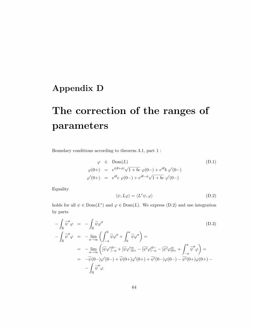
Appendix D

The correction of the ranges of

parameters

Boundary conditions according to theorem 3.1, part 1 :

ϕ ∈ Dom(L) (D.1)

ϕ(0+) = ei(θ+φ)√

1 + bc ϕ(0−) + eiθb ϕ′(0−)

ϕ′(0+) = eiθc ϕ(0−) + eiθ−φ√

1 + bc ϕ′(0−)

Equality〈ψ,Lϕ〉 = 〈L∗ψ,ϕ〉 (D.2)

holds for all ψ ∈ Dom(L∗) and ϕ ∈ Dom(L). We express (D.2) and use integrationby parts

−∫

Rψ′′ϕ = −

∫Rψϕ′′ (D.3)

−∫

Rψ′′ϕ = − lim

a→∞

(∫ 0

−aψϕ′′ +

∫ a

0ψϕ′′

)=

= − lima→∞

([ψϕ′]0−−a + [ψϕ′]a0+ − [ψ′ϕ]0−−a − [ψ′ϕ]a0+ +

∫ a

−aψ′′ϕ

)=

= −ψ(0−)ϕ′(0−) + ψ(0+)ϕ′(0+) + ψ′(0−)ϕ(0−)− ψ′(0+)ϕ(0+)−

−∫

Rψ′′ϕ.

64

Inserting the boundary conditions for ϕ ∈ Dom(L) into (D.4) yields

ϕ′(0−)[ψ(0−)− ψ(0+)ei(φ−θ)

√1 + bc+ ψ′(0+)e−iθb

]+ (D.4)

+ϕ(0−)[−ψ′(0−)− ψ(0+)e−iθc+ ψ′(0+)e−i(φ+θ)

√1 + bc

]= 0,

where boundary values of ϕ at x→ 0− may be chosen arbitrarily (we have alreadyused (D.2) ). We conclude that ψ ∈ Dom(L∗) must satisfy

ψ(0−) = ψ(0+)ei(φ−θ)√

1 + bc− ψ′(0+)e−iθb (D.5)

ψ′(0−) = −ψ(0+)e−iθc+ ψ′(0+)e−i(φ+θ)√

1 + bc. (D.6)

If L is P-pseudo-Hermitian then L∗ = PLP and hence Dom(L∗) = PDom(L).Boundary conditions corresponding to PDom(L) read

ψ(0−) = ψ(0+)ei(φ+θ)√

1 + bc− ψ′(0+)eiθb (D.7)

ψ′(0−) = −ψ(0+)eiθc+ ψ′(0+)e−i(φ−θ)√

1 + bc. (D.8)

Hence the equality of the domains is satisfied only if θ = 0.

65

Bibliography

[1] Albeverio, S., Fei, S. M., and Kurasov, P. Point Interactions: PT-Hermiticity and Reality

of the Spectrum. Letters in Mathematical Physics 59 (2002), 227–242.

[2] Albeverio, S., Gesztesy, F., Hegh-Krohn, R., and Holden, H. Solvable Models in

Quantum Mechanics. Springer, New York, 1988.

[3] Albeverio, S., and Kuzhel, S. One-dimensional Schrodinger operators with P-symmetric

zero-range potentials. Journal of Physics A: Mathematical and General 38, 22 (2005), 4975–

4988.

[4] Bagchi, B., Mallik, S., and Quesne, C. PT-symmetric square well and the associated

SUSY hierarchies. Modern Physics Letters A 17 (2002), 1651–1664.

[5] Bender, C. M., and Boettcher, S. Real Spectra in Non-Hermitian Hamiltonians Having

PT Symmetry. Physical Review Letters 80 (1998), 5243–5246.

[6] Bender, C. M., Boettcher, S., and Meisinger, P. PT-Symmetric Quantum Mechanics.

Journal of Mathematical Physics 40 (1999), 2201–2229.

[7] Bender, C. M., Brody, D. C., and Jones, H. F. Complex Extension of Quantum Mechan-

ics. Physical Review Letters 89 (2002), 270401.

[8] Bender, C. M., Brody, D. C., and Jones, H. F. Must a Hamiltonian be Hermitian?

American Journal of Physics 71 (2003), 1095–1102.

[9] Bender, C. M., Brody, D. C., and Jones, H. F. Erratum: Complex Extension of Quantum

Mechanics. Physical Review Letters 92 (2004), 119902.

[10] Blank, J., Exner, P., and Havlıcek, M. Hilbert Space Operators in Quantum Physics

(Computational and Applied Mathematical Physics). American Institute of Physics, 1999.

[11] Borisov, D., and Krejcirık, D. PT-symmetric waveguide. 0707.3039, 2007.

[12] Caliceti, E., Graffi, S., and Maioli, M. Perturbation theory of odd anharmonic oscilla-

tors. Communications in Mathematical Physics 75 (1980), 51–66.

[13] Dieudonne, J. Quasi-Hermitian operators. Proceedings Of The International Symposium on

Linear Spaces (July 1961), 115–123.

66

[14] Dirac, P. A. M. The Physical Interpretation of Quantum Mechanics. Proceedings of the

Royal Society of London A 180, 980 (1942), 1–40.

[15] Dunford, N., and Schwartz, J. T. Linear Operators Part III Spectral Operators. Wiley-

Interscience, 1971.

[16] Edmunds, D. E., and Evans, W. D. Spectral Theory and Differential Operators (Oxford

Mathematical Monographs). Oxford University Press, USA, 1987.

[17] Garcia, S. R. The Eigenstructure of Complex Symmetric Operators. Proceedings of the

Sixteenth International Conference on Operator Theory and Applications (IWOTA 16) 179

(2008), 169–183.

[18] Garcia, S. R., and Putinar, M. Complex symmetric operators and applications. Transac-

tions Of The American Mathematical Society 358 (2006), 1285–1315.

[19] Gesztesy, F., and Tkachenko, V. A Criterion for Hill Operators to be Spectral Operators

of Scalar Type. math/0610502, 2006.

[20] Kato, T. Perturbation theory for linear operators. Springer-Verlag, 1966.

[21] Koosis, P. Introduction to Hp Spaces. Cambridge University Press, 1980.

[22] Krejcirık, D., Bıla, H., and Znojil, M. Closed formula for the metric in the Hilbert

space of a PT-symmetric model. Journal of Physics A: Mathematical and General 39 (2006),

10143–10153.

[23] Kretschmer, R., and Szymanowski, L. Quasi-Hermiticity in infinite-dimensional Hilbert

spaces. Physics Letters A 325 (2004), 112.

[24] Levai, G., and Znojil, M. The interplay of supersymmetry and PT symmetry in quantum

mechanics: a case study for the Scarf II potential. Journal of Physics A: Mathematical and

General 35 (2002), 8793 – 8804.

[25] Malamud, M. A criterion for a closed operator to be similar to a selfadjoint operator.

Ukrainian Mathematical Journal, English translation 37 (1985), 41–48.

[26] Mostafazadeh, A. Pseudo-Hermiticity versus PT Symmetry I: The necessary condition for

the reality of the spectrum of a non-Hermitian Hamiltonian. Journal of Mathematical Physics

43 (2002), 205–214.

[27] Mostafazadeh, A. Pseudo-Hermiticity versus PT-Symmetry II: A complete characterization

of non-Hermitian Hamiltonians with a real spectrum. Journal of Mathematical Physics 43

(2002), 2814–2816.

[28] Mostafazadeh, A. Pseudo-Hermiticity versus PT-Symmetry III: Equivalence of pseudo-

Hermiticity and the presence of antilinear symmetries. Journal of Mathematical Physics 43

(2002), 3944–3951.

[29] Mostafazadeh, A. Delta-Function Potential with a Complex Coupling. Journal of Physics

A: Mathematical and General 39 (2006), 13495–13506.

67

[30] Mostafazadeh, A. Is Weak Pseudo-Hermiticity Weaker than Pseudo-Hermiticity? Journal

of Mathematical Physics 47 (2006), 092101.

[31] Mostafazadeh, A. Metric Operators for Quasi-Hermitian Hamiltonians and Symmetries of

Equivalent Hermitian Hamiltonians. Preprint 0707.3075, 2007.

[32] Naboko, S. Conditions for similarity to unnitary and selfadjoint operators. Functional Anal-

ysis and its Applications 18 (1984), 13–22.

[33] Nagasawa, T., Sakamoto, M., and Takenaga, K. Supersymmetry in quantum mechanics

with point interactions. Physics Letters B 562 (2003), 358–364.

[34] Pauli, W. On Dirac’s New Method of Field Quantization. Reviews of Modern Physics 15, 3

(1943), 175–207.

[35] Reed, M., and Simon, B. Methods of Modern Mathematical Physics, Vol. 1: Functional

Analysis, revised and enlarged edition ed. Academic Press, 1980.

[36] Rudin, W. Functional Analysis. McGraw-Hill Book Company, 1973.

[37] Scholtz, F. G., Geyer, H. B., and Hahne, F. J. W. Quasi-Hermitian operators in quantum

mechanics and the variational principle. Annals of Physics 213 (1992), 74–101.

[38] Scolarici, G., and Solombrino, L. On the pseudo-Hermitian nondiagonalizable Hamilto-

nians. quant-ph/0211161, 2002.

[39] Siegl, P. Supersymmetric quasi-Hermitian Hamiltonians with point interactions on a loop.

Journal of Physics A: Mathematical and Theoretical 41 (2008), to appear.

[40] Solombrino, L. Weak pseudo-Hermiticity and antilinear commutant. quant-ph/0203101,

2002.

[41] van Casteren, J. A. Operators similar to unitary or selfadjoint ones. Pacific Journal of

Mathematics 104, 1 (1983), 241–255.

[42] Vilenkin, N. Y., Gorin, E. A., Kostyuchenko, A. G., Krasnosefskii, M. A., Krein,

S. G., Maslov, V. P., Mityagin, B. S., Petunin, Y. I., Rutitskii, Y. B., Sobolev,

V. I., Stetsenko, V. Y., Faddeev, L. D., and Tsitlanadze, E. S. Functional Analysis.

Wolters-Noordhoff Publishing, 1972.

[43] Williams, J. P. Operators Similar to Their Adjoints. Proceedings of the American Mathe-

matical Society 20 (1969), 121–123.

[44] Znojil, M. Private communication.

[45] Znojil, M. Conditional observability. Physics Letters B 650 (2007), 440–446.

[46] Znojil, M. Maximal couplings in PT-symmetric chain models with the real spectrum of

energies. Journal of Physics A: Mathematical and Theoretical 40, 18 (2007), 4863–4875.

[47] Znojil, M. A return to observability near exceptional points in a schematic PT-symmetric

model. Physics Letters B 647 (2007), 225–230.

68

[48] Znojil, M. Tridiagonal PT -symmetric N-by-N Hamiltonians and a fine-tuning of their ob-

servability domains in the strongly non-Hermitian regime. Journal of Physics A: Mathematical

and Theoretical 40, 43 (2007), 13131–13148.

[49] Znojil, M., and Jakubsky, V. Solvability and PT -symmetry in a double-well model with

point interactions. Journal of Physics A: Mathematical and General 38, 22 (2005), 5041–5056.

69