quasi-experimental workshop - northwestern university · quasi-experimental workshop tom cook and...
TRANSCRIPT

Quasi-Experimental Workshop
Tom Cook and Will Shadish
Supported by Spencer Foundation

Introduction: Purposes• Briefly describe the sorry current state of causal
research in education• Learn why the randomized experiment is so
preferred when it is feasible• Learn better quasi-experimental designs and
principles of creating new designs• Improve your own causal research projects
through discussion with Will and Tom• Disseminate better practices when go home• Have fun, eat well, meet interesting new people

Introductions: People
StaffLogic for selecting youNow we will go around. Please give us Your name and affiliationPrior experience with experiments, withquasi-experiments, and with non-experimental methods used to draw causal conclusions
Decorum
No dress codePlease interrupt for clarificationEngage instructors in side conversations at
breaks and mealsNo titles, only first names

Schedule by Day
• Morning session, lunch period, afternoon, rest, dinner
• Lunch to meet others, let off steam, or discuss your own projects with Tom or Will
• Rest period to catch up on home, meet Tom or Will, discuss material with others
• Dinners are to have fun and socialize

And at the End of the Workshop
• We will provide a web site and email addresses for followup
• Provide you with finalized sets of powerpoint slides (since we do tend to change them at each workshop a little).

• The Current State of the Causal Art in Education Research

Education leads the other Social Sciences in Methods for:
• Meta-Analysis• Hierarchical Linear Modeling• Psychometrics• Analysis of Individual Change• So these next 5 days do not entail an
indictment of education research methods writ large
• Only of its methods for identifying what works, identifying casual relationships

State of Practice in Causal Research in Education
• Theory and research suggest best methods for causal purposes. Yet
• Low prevalence of randomized experiments--Ehri; Mosteller
• Low prevalence of Regression-discontinuity• Low prevalence of interrupted time series• Low prevalence of studies combining control
groups, pretests and sophisticated matching• High prevalence of weakest designs: pretest-
posttest only; non-equivalent control group without a pretest; and even with it.
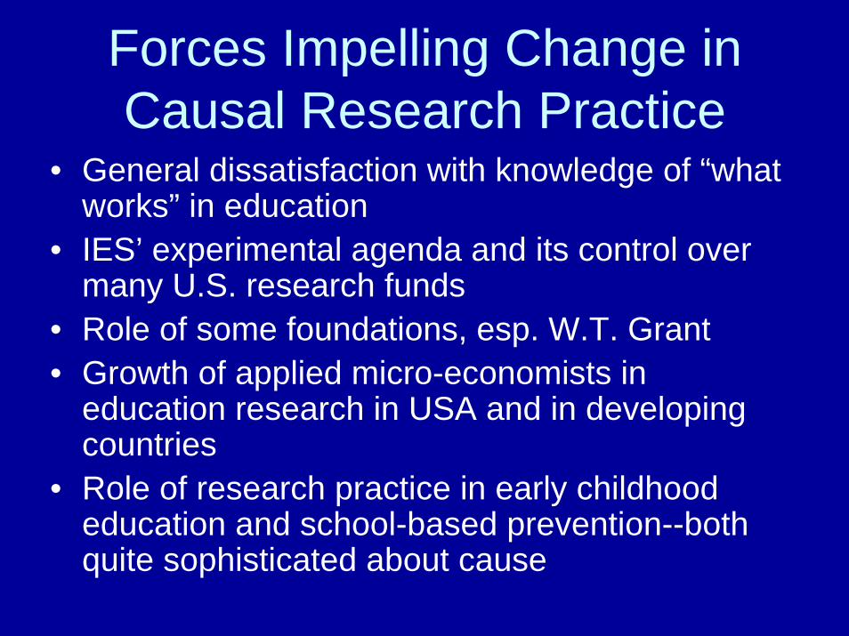
Forces Impelling Change in Causal Research Practice
• General dissatisfaction with knowledge of “what works” in education
• IES’ experimental agenda and its control over many U.S. research funds
• Role of some foundations, esp. W.T. Grant• Growth of applied micro-economists in
education research in USA and in developing countries
• Role of research practice in early childhood education and school-based prevention--both quite sophisticated about cause
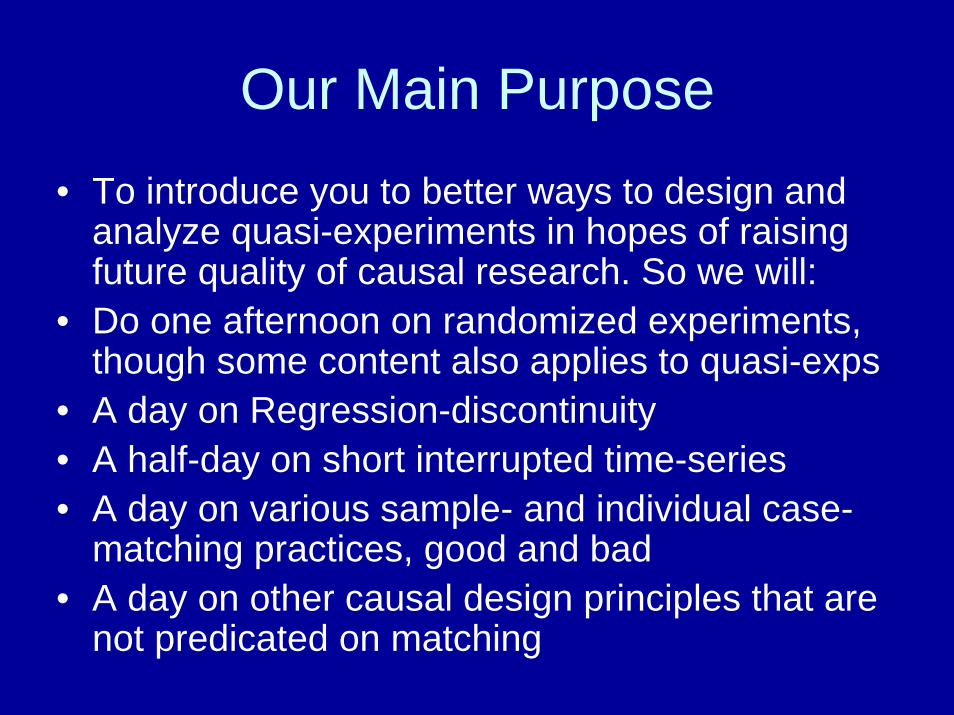
Our Main Purpose• To introduce you to better ways to design and
analyze quasi-experiments in hopes of raising future quality of causal research. So we will:
• Do one afternoon on randomized experiments, though some content also applies to quasi-exps
• A day on Regression-discontinuity• A half-day on short interrupted time-series• A day on various sample- and individual case-
matching practices, good and bad• A day on other causal design principles that are
not predicated on matching

Terminology to Keep us on Track
• Experimentation - deliberate intrusion into an ongoing process to identify effects of that intrusion--contrast with causal but non-experimental study as with surveys
• A non-experimental causal study seeks to draw conclusions about some causal agent that is neither deliberately manipulated nor suddenly intrusive into some ongoing process--examples

Terminology
• Randomized experiments involve assignment to treatment and comparison groups based on chance--examples
• Quasi-experiments involve assignment to treatment not based on chance--examples
• Natural experiment denotes some sudden and non-researcher controlled intrusion into an ongoing process--examples

Today we will
• Discuss what we mean by causation• Discuss threats to validity, esp. internal
validity• Analyze the randomized experiment as the
archetypal causal study• Discuss the limitations to doing
experiments in real school settings• Discuss ways of circumventing these
limitations

Some Working Conceptions of Causation

Activity or Manipulability Theory
• What is it? • Some examples from daily life and science• Why it is important for practice and policy• How it relates to experimentation• Illustrating its major limitations through
confrontation with other theories of causation

Mackie’s INUS ConditionalInsufficient but Necessary Parts of Unnecessary but Sufficient conditions for an Effect
• An elaboration of this with the matchstick and fire example
• Its implications for the contingency-ladenness of complete causal knowledge versus the limited contingent nature of the results from any one experiment or quasi-experiment
• Raises the specter of knowing when the causal conclusion from any one experimental study is dependable, given it is but part of a whole

Cronbach’s UTOS Formulation• Studies require Units, Treatments, Outcomes
(Observations), Settings -- and also Times• These condition the results of any one causal
claim from an experiment -- some examples• Implication 1. Identify causal mediating
processes• Implication 2. The unit of progress is more likely
to be a review than a single study• But each requires studies whose causal
conclusions we can trust! Hence this workshop.

Another Way of Saying this (1)• Science values explanatory causal knowledge
over study-specific descriptions of a causal relationship from some A to B
• Public policy should too because this increases dependability of application
• However, explanatory causal knowledge assumes stable knowledge of the causal descriptions it contains.
• So experimentation is a way station to where we would prefer to be and want to be in the future

Another Way of Saying this (2)
• Reviews allow us to establish dependability of a causal connection provided that the UTOS sampling frame is heterogeneous
• Reviews allow us to identify some specific moderator and mediator variables
• But reviews require individual causal conclusions we trust. Hence this workshop

• Now we turn to the best explicated theory of descriptive causal practice for the social sciences:
Rubin’s Causal Model


Rubin’s Counterfactual Model
• At a conceptual level, this is a counterfactual model of causation. – An observed treatment given to a person. The
outcome of that treatment is Y(1)– The counterfactual is the outcome that would have
happened Y(0) if the person had not received the treatment.
– An effect is the difference between what did happen and what would have happened:
Effect = Y(1) – Y(0). • Unfortunately, it is impossible to observe the
counterfactual, so much of experimental design is about finding a credible source of counterfactual inference.

Rubin’s Model: Potential Outcomes
• Rubin often refers to this model as a “potential outcomes” model.
• Before an experiment starts, each participant has two potential outcomes, – Y(1): Their outcome given treatment– Y(0): Their outcome without treatment
• This can be diagrammed as follows:

Rubin’s Potential Outcomes ModelUnits Potential Outcomes Causal Effects
Treatment Control1 Y1(1) Y1(0) Y1(1) – Y1(0)
i Yi(1) Yii(0) Yi(1) – Yi(0)
N YN(1) YN(0) YN(1) – YN(0)
MM M
MMM
)1(Y )0(Y
Under this model, we can get a causal effect for each person.
)0()1( YY −
And we can get an average causal effect as the difference between group means.

Rubin’s Potential Outcomes Model
Units Potential Outcomes Causal EffectsTreatment Control
1 Y1(1) Y1(0) Y1(1) – Y1(0)
i Yi(1) Yii(0) Yi(1) – Yi(0)
N YN(1) YN(0) YN(1) – YN(0)
MM M
MMM
)1(Y )0(YUnfortunately, we can only observe one of the two potential outcomes for each unit. Rubin proposed that we do so randomly, which we accomplish by random assignment:
)0()1( YY −

Rubin’s Potential Outcomes Model
Units Potential Outcomes Causal EffectsTreatment Control
1 Y1(1)
i Yii(0)
N YN(1)
MM M
MMM
)0()1( YY −)0(YThe cost of doing this is that we can no longer estimate individual causal effects. But we can still estimate Average Causal Effect (ACE) as the difference between the two group means. This estimate is unbiased because the potential outcomes are missing completely at random.
)1(Y

Rubin’s Model and Quasi-Experiments
• The aim is to construct a good source of counterfactual inference given that we cannot assign randomly, for example– Well-matched groups– Persons as their own controls
• Rubin has also created statistical methods for helping in this task:– Propensity scores– Hidden bias analysis

Is Rubin’s Model Universally Applicable?
• Natural Sciences invoke causation and they experiment, but they rarely use comparison groups for matching purposes
• They pattern-match instead, creating either a• Very specific hypothesis as a point prediction; or • Very elaborate hypothesis that is then tested via
re-application and removal of treatment under experimenter control
• We will later use insights from this notion to construct a non-matching approach to causal inference in quasi-experiments to complement matching approaches

Very Brief Exigesis of Validity
• This goes over some well known ground• But it forces us to be explicit about the
issues on which we prioritize in this workshop

Validity• We do (or read about) a quasi-experiment that
gathered (or reported) data• Then we make all sorts of inferences from the
data– About whether the treatment worked– About whether it might work elsewhere
• The question of validity is the question of the truth of those inferences.
• Campbell’s validity typology is one way to organize our thinking about inferences.

Campbell’s Validity Typology
• As developed by Campbell (1957), Campbell & Stanley (1963), Cook & Campbell (1979), with very minor changes in Shadish, Cook & Campbell (2002)– Internal Validity– Statistical Conclusion Validity– Construct Validity– External Validity
• Each of the validity types has prototypical threats to validity—common reasons why we are often wrong about each of the four inferences.

Internal Validity• Internal Validity: The validity of inferences about
whether observed covariation between A (the presumed treatment) and B (the presumed outcome) reflects a causal relationship from A to B, as those variables were manipulated or measured.
• Or more simply—did the treatment affect the outcome?
• This will be the main priority in this workshop.

Threats to Internal Validity1. Ambiguous Temporal Precedence2. Selection3. History4. Maturation5. Regression6. Attrition7. Testing8. Instrumentation9. Additive and Interactive Effects of Threats to Internal
ValidityThink of these threats as specific kinds of
counterfactuals—things that might have happened to the participants if they had not
received treatment.

Statistical Conclusion Validity
• Statistical Conclusion Validity: The validity of inferences about the correlation (covariation) between treatment and outcome.
• Closely tied to Internal Validity– SCV asks if the two variables are correlated– IV asks if that correlation is due to causation

Threats to Statistical Conclusion Validity
1. Low Statistical Power (very common)2. Violated Assumptions of Statistical Tests (especially problems of nesting—students nested in classes)
3. Fishing and the Error Rate Problem4. Unreliability of Measures5. Restriction of Range6. Unreliability of Treatment Implementation7. Extraneous Variance in the Experimental Setting8. Heterogeneity of Units9. Inaccurate Effect Size Estimation
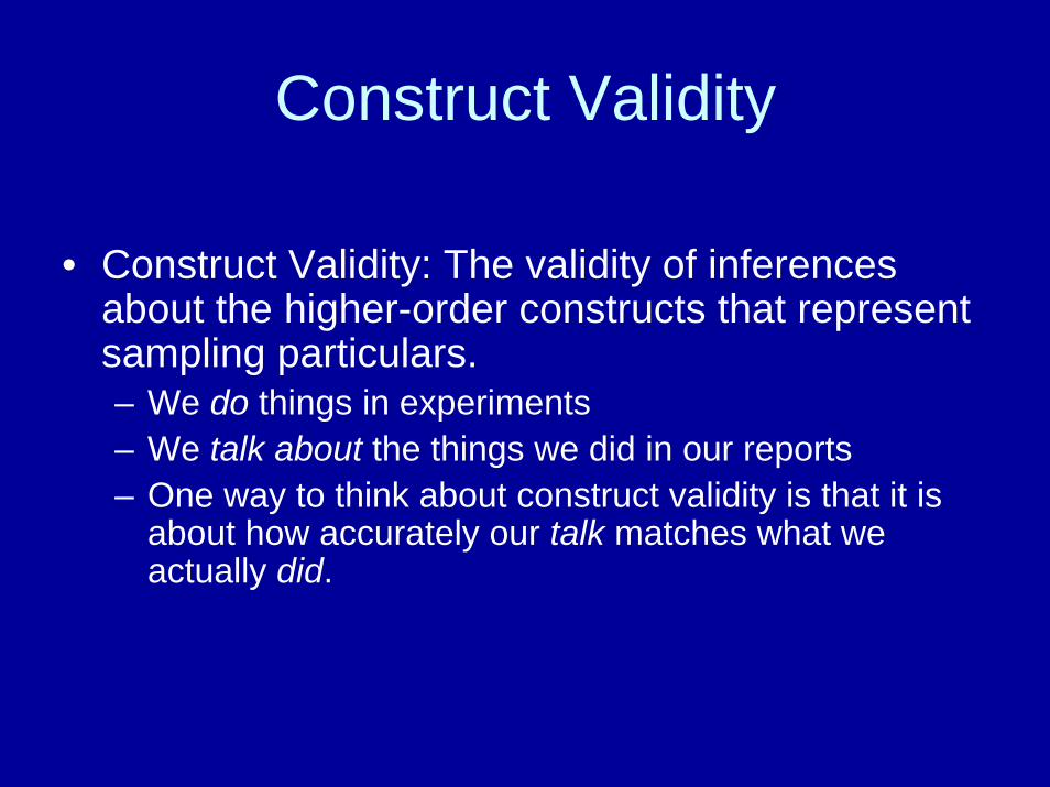
Construct Validity
• Construct Validity: The validity of inferences about the higher-order constructs that represent sampling particulars. – We do things in experiments– We talk about the things we did in our reports– One way to think about construct validity is that it is
about how accurately our talk matches what we actually did.

External Validity
• External Validity: The validity of inferences about whether the cause-effect relationship holds over variation in persons, settings, treatment variables, and measurement variables.
• Always the “stepchild” in Campbell’s work, Cook has developed a theory of causal generalization addressing both construct and external validity.
• But that is another workshop.

Validity Priorities for This Workshop
Main Focus is Internal ValidityStatistical Conclusion Validity: Because it is so closely tied
to Internal ValidityRelatively little focus
Construct Validity External Validity

Randomized Experiments with Individual Students and with Clusters of Classrooms or Schools

Randomized Control Trials
1. Logic of random assignment2. Assumptions of RCTs3. Current Efforts to Promote Experiments
in Education4. Special Technical Issues with Schools
and Classrooms

What is an Experiment?
• The key feature common to all experiments is to deliberately manipulate a cause in order to discover its effects
• Note this differentiates experiments from – Case control studies, which first identify an
effect, and then try to discover causes, a much harder task

Random Assignment
• Any procedure that assigns units to conditions based only on chance, where each unit has a nonzero probability of being assigned to a condition – Coin toss– Dice roll– Lottery– More formal methods (more shortly)

What Random Assignment Is Not
• Random assignment is not random sampling– Random sampling is rarely feasible in
experiments• Random assignment does not require that
every unit have an equal probability of being assigned to conditions– You can assign unequal proportions to
conditions

Equating on Expectation
• Randomization equates groups on expectation for all observed and unobserved variables, not in each experiment– In quasi-experiments matching only equates on observed
variables. • Expectation: the mean of the distribution of all
possible sample means resulting from all possible random assignments of units to conditions – In cards, some get good hands and some don’t (luck of the
draw)– But over time, you get your share of good hands
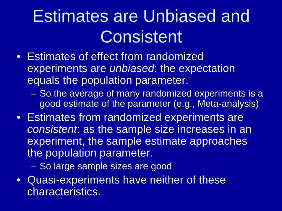
Estimates are Unbiased and Consistent
• Estimates of effect from randomized experiments are unbiased: the expectation equals the population parameter.– So the average of many randomized experiments is a
good estimate of the parameter (e.g., Meta-analysis)• Estimates from randomized experiments are
consistent: as the sample size increases in an experiment, the sample estimate approaches the population parameter. – So large sample sizes are good
• Quasi-experiments have neither of these characteristics.

Randomized Experiments and The Logic of Causal Relationships
• Logic of Causal Relationships– Cause must precede effect– Cause must covary with effect– Must rule out alternative causes
• Randomized Experiments Do All This– They give treatment, then measure effect– Can easily measure covariation– Randomization makes most other causes less likely
• Quasi-experiments are problematic on the third criterion.• But no method matches this logic perfectly (e.g., attrition
in randomized experiments).

Assumptions on which a Treatment Main Effect depends
• Posttest group means will differ, but they are causally interpretable only if:
• The assignment is proper, so that pretest and other covariate means do not differ on observables on expectation (and in theory on unobservables)
• There is no differential attrition, and so the attrition rate and profile of remaining units is constant across treatment groups
• There is no contamination across groups, which is relevant for answering questions about treatment-on-treated but not about intent to treat.

Advantages of Experiments
• Unbiased estimates of effects• Relatively few, transparent and testable
assumptions• More statistical power than alternatives• Long history of implementation in health,
and in some areas of education• Credibility in science and policy circles
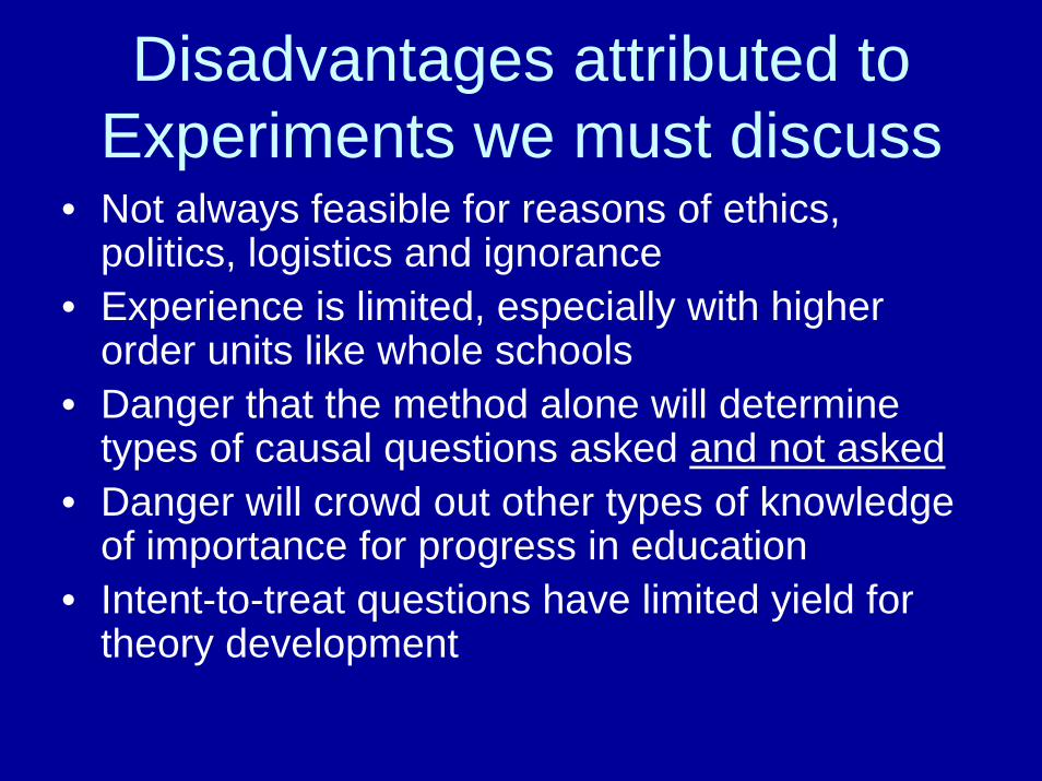
Disadvantages attributed to Experiments we must discuss
• Not always feasible for reasons of ethics, politics, logistics and ignorance
• Experience is limited, especially with higher order units like whole schools
• Danger that the method alone will determine types of causal questions asked and not asked
• Danger will crowd out other types of knowledge of importance for progress in education
• Intent-to-treat questions have limited yield for theory development

Promotion of RCTs in American Education Today

RA in American Educational Research Today
• IES, NSF, NIH and Foundations• IES Rhetoric about Causation and Causal
Methods• Reality in terms of Funding Decisions

IES Causal Programs
• National Evaluations mandated by Congress or some Title and done by contract research firms
• Program Announcements for Field-Initiated Studies mostly done in universities
• Training and Center Grants to universities• What Works Clearinghouse• Regional Labs• SREE - Society for Research in Educational
Effectiveness
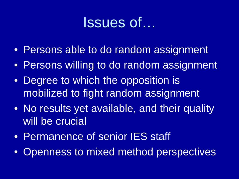
Issues of…
• Persons able to do random assignment• Persons willing to do random assignment• Degree to which the opposition is
mobilized to fight random assignment• No results yet available, and their quality
will be crucial• Permanence of senior IES staff• Openness to mixed method perspectives

Analyses Taking Implementation into Account
• An intent-to-treat analysis (ITT)• An analysis by amount of treatment
actually received (TOT)• Need to construct studies that give
unbiased inference about each type of treatment effect.

Partial Treatment Implementation
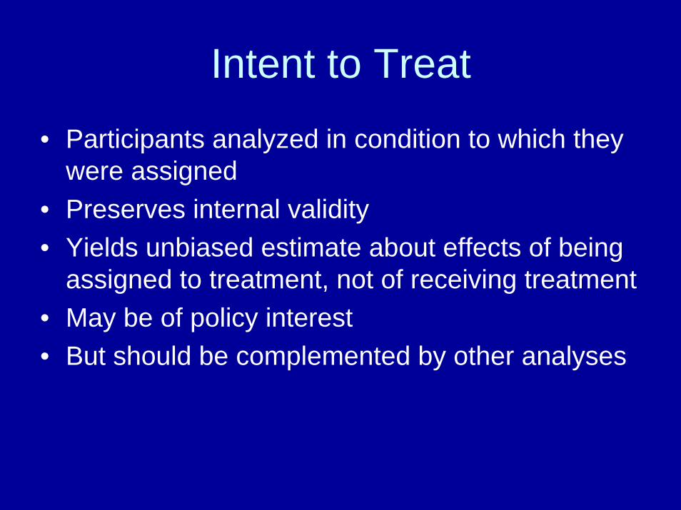
Intent to Treat
• Participants analyzed in condition to which they were assigned
• Preserves internal validity• Yields unbiased estimate about effects of being
assigned to treatment, not of receiving treatment • May be of policy interest• But should be complemented by other analyses

Analysis by Treatment Received
• Compare outcomes for those who received treatment to outcomes for those who did not
• Estimates effects of treatment receipt• But is quasi-experimental• Rarely a good option by itself

Instrumental Variables Analysis• Angrist, Imbens, Rubin JASA 1996• In economics, an instrument is a variable
or set of variables is correlated with outcome only through an effect on other variables (in this case, on treatment)
• Can use the instrument to obtain an unbiased estimate of effect
Instrument Treatment Outcome

Instrumental Variables Analysis• Use random assignment as an instrument for
incomplete treatment implementation• Yields unbiased estimate of the effects of receipt
of treatment
• Random assignment is certainly related to treatment, but it is unrelated to outcome except through the treatment.
Random Assignment
Treatment Outcome

Example: The Effects of Serving in the Military on Death
• Lottery randomly assigned people to being eligible for the draft. – Intent to treat analysis would assess the effects of
being eligible for the draft on death
• This is a good randomized experiment yielding an unbiased estimate
Lottery: Eligible for Draft or Not
Death

Example continued• But that is not the question of interest
– Not all those eligible for the draft entered the military (not all those assigned to treatment received it).
• Some who were draft eligible were never drafted• Some who were not eligible chose to enlist
– We could compare the death rates for those who actually entered the military with those who did not (we could compare those who received treatment to those who did not):
– But this design is quasi-experimental
Entered Military or Not Death

Example: Instrumental Variable Analysis
• Random assignment is an instrument because it can only affect the outcome through the treatment.
• That is, being randomly assigned to being draft eligible only affects death if the person actually joins the military.
Lottery: Draft Eligible or not Entered
Military or NotDied

Analysis for binary outcome and binary treatment implementation
• 35.3% draft eligible served in military• 19.4% not eligible served in military• The lottery (random assignment) caused 15.9%
to serve in the military (normal randomized experiment)
• 2.04% draft eligible died• 1.95% not eligible died• Draft eligible caused 0.09% to die• Causal effect of serving in military on death
among those participating in the lottery is .0009/.159 = .0058 = .56%

Assumptions
1. One person’s outcomes do not vary depending on the treatment someone else is assigned
2. The causal effects of assignment both on receipt and on outcome can be estimated using standard intent-to-treat analyses
3. Assignment to treatment has a nonzero effect on receipt of treatment
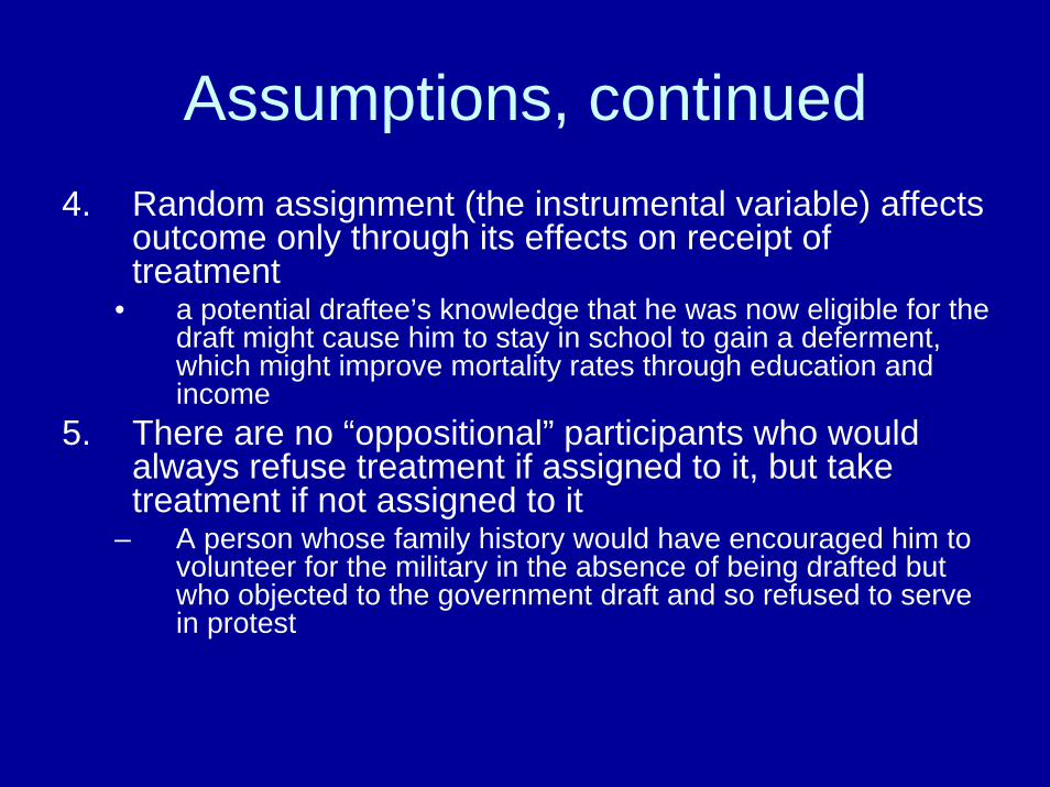
Assumptions, continued4. Random assignment (the instrumental variable) affects
outcome only through its effects on receipt of treatment
• a potential draftee’s knowledge that he was now eligible for the draft might cause him to stay in school to gain a deferment, which might improve mortality rates through education and income
5. There are no “oppositional” participants who would always refuse treatment if assigned to it, but take treatment if not assigned to it
– A person whose family history would have encouraged him to volunteer for the military in the absence of being drafted but who objected to the government draft and so refused to serve in protest

More on Angrist et al.
• Extensions to – Variable treatment intensity– Quasi-experiments– Continuous outcomes
• An area rapidly developing

Issues of Nesting and Clusters, most of which is also relevant to Quasi-Experiments

Units and Aggregate Units• Can randomly assign:
– Units (e.g., children, households)– Aggregates (e.g., classrooms, neighborhoods)
• Why we use aggregates: – When the aggregate is of intrinsic interest (e.g.,
effects of whole school reform)– To avoid treatment contamination effects within
aggregates.– When treatment cannot be restricted to individual
units (e.g., city wide media campaigns)

The Problem with Aggregates• Most statistical procedures assume (and require) that
observations (errors) be independent of each other.• When units are nested within aggregates, units are
probably not independent– If units are analyzed as if they were independent, Type I error
skyrockets• E.g., an intraclass correlation of .001 can lead to a Type I error rate
of α > .20!
• Further, degrees of freedom for tests of the treatment effect should now be based on the number of aggregates, not the number of persons.

What Creates Dependence?
• Aggregates create dependence by– Participants interacting with each other– Exposure to common influences (e.g,.
Patients nested within physician practices)• Both these problems are greater the
longer the group members have been interacting with each other.

Making an Unnecessary Independence Problem
• Individual treatment provided in groups for convenience creates dependence the more groups members interact and are exposed to same influences.
• Empirically Supported Treatments or Type I errors?– About of a third of ESTs provide treatment in groups– When properly reanalyzed, very few results were still
significant.

Some Myths about Nesting• Myth: Random assignment to aggregates solves the
problem.– This does not stop interacting or common influences
• Myth: All is OK if the unit of assignment is the same as the unit of analysis.– That is irrelevant if there is nesting.
• Myth: You can test if the ICC = 0, and if so, ignore aggregates.– That test is a low power test
• Myth: No problem if randomly assign students to two groups within one classroom.– Students are still interacting and exposed to same influences

The Worst Possible Case
• Random assignment of one aggregate (e.g., a class) per condition– The problem is that class and condition are
completely confounded, leaving no degrees of freedom with which to estimate the effect of the class.
– This is true even if you randomly assign students to classes first.

What to Do?• Avoid using one aggregate per condition• Design to ensure sufficient power--more to come later
– have more aggregates with fewer units per aggregate– randomly assign from strata– use covariates or repeated measure
• Analyze correctly– On aggregate means (but low power, and loses individual data)– Using multilevel modeling (preferred)
• Increase degrees of freedom for the error term by borrowing information about ICCs from past studies
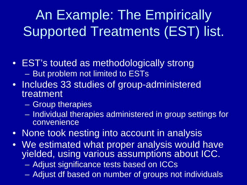
An Example: The Empirically Supported Treatments (EST) list.
• EST’s touted as methodologically strong– But problem not limited to ESTs
• Includes 33 studies of group-administered treatment– Group therapies– Individual therapies administered in group settings for
convenience• None took nesting into account in analysis• We estimated what proper analysis would have
yielded, using various assumptions about ICC. – Adjust significance tests based on ICCs– Adjust df based on number of groups not individuals

Table 1Equations for adjusting Effects
Estimators.
t-test ICCmtt
o
unadjadj
)1(1 −+=
F-test for ANOVA Fadj =Funadj
1+(mo−1)ICC
Chi-Square ICCmo
unadjadj
)1(1
22−+
=χχ
Note. Adapted from Rooney (1992). m=number of members per group, ICC=Intraclass Correlation.

Results• After the corrections, only 12.4% to 68.2% of tests that
were originally reported as significant remained significant
• When we considered all original tests, not just those that were significant, 7.3% to 40.2% of tests remained significant after correction
• The problem is even worse, because most of the studies tested multiple outcome variables without correcting for alpha inflation
• Of the 33 studies, 6-19 studies no longer had anysignificant results after correction, depending on assumptions

332332N =
CorrectedReported
Deg
rees
of F
reed
om
200
100
0
332332332332N =
Corrected F ICC=.30Corrected F ICC=.15
Corrected F ICC=.05Reported F
F
80
60
40
20
0
119119N =
CorrectedReported
Deg
rees
of F
reed
om
200
100
0119119119119N =
Corrected F ICC=.30Corrected F ICC=.15
Corrected F ICC=.05Reported F
F
50
40
30
20
10
0
For all N = 332 t- and F-tests
For N = 119 omnibus t- and F-tests with exact information
Other Issues at the Cluster Level
• Getting Agreement• Sample Size and Power• Contamination

Cluster Level Random Assignment- Getting Agreement• High rate of RA in preschool studies of
achievement and in school-based studies of prevention, but not in school-based studies of achievement. What does this imply?
• Cook’s war stories - PGC; Chicago; Detroit• Grant Fdn. Resources• Experiences at Mathematica• District-level brokers

Estimating the Needed Sample Size
• Formulating the question: How many schools are needed for ES of .20, with p < .05, power .80, balanced design and > 50 students per school.
• Why .20? Why .05, why .80. Why balanced? What role does the N of students play?

Key Considerations• Estimating the cluster effect via the
unconditional ICC, that part of the totalvariation that is within schools
• Estimating the conditional ICC, what the difference between schools is after covariates have been used to “explain” some of the between-school variation
• It is the conditional ICC that determines power and hence the sample size needed
• Two examples, one local and the other national

Example 1: Kentucky
• An achievement study• A school-level question• A limited budget• One year of prior achievement data at
both the school and student levels• Given these data, and traditional power
assumptions, how many schools needed to detect an effect of .20?
• We use J for schools and N for students
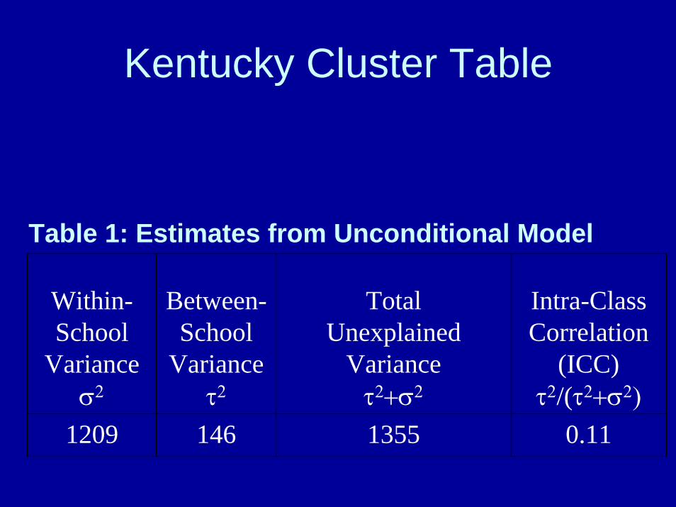
Kentucky Cluster Table
Within-School
Varianceσ2
Between-School
Varianceτ2
Total Unexplained
Varianceτ2+σ2
Intra-Class Correlation
(ICC)τ2/(τ2+σ2)
1209 146 1355 0.11
Table 1: Estimates from Unconditional Model

Table 2: Required J for the Unconditional Model
Unconditional Effect Size Required J
0.20 94
0.25 61
0.30 43

What is the School Level Covariate like?
For reading, the obtained covariate-outcome r is .85--the usual range in other studies is .70 to .95
As corrected in HLM this value is .92What happens when this pretest school-
level covariate is used in the model?

Table 3: Estimates from Conditional Model (CTBS as
Level-2 Covariate)
WithinSchool
Varianceσ2
BetweenSchool
VarianceΤ2
Total Unexplained
Varianceτ2+σ2
Intra-Class Correlation (ICC)
τ2/(τ2+σ2)1210 21.6 1231.6 0.0175

What has happened?
• The total unexplained variation has shrunk from 1355 to 1232--why?
• The total between-school variation has shrunk from 146 to 26--why?
• So how many school are now needed for the same power?

Table 4: Required J for Two Level Unconditional and
Conditional Models
EffectSize
Required JNo Covariate
Required JWith Covariate
0.20 94 22
0.25 61 15
0.30 43 12

How does these Values Compare?
• The work of Bloom and Raudenbush with 5 ad hoc chosen school districts:
• The work of Hedges with nationally representative data where m is his term for sample size at the school level (not J)

National Estimates from HedgesGrade Covariates m=10 m=15 m=20 m=25 m=301 None 0.67 0.54 0.46 0.41 0.37
Pretest 0.32 0.25 0.22 0.19 0.18
5 None 0.70 0.56 0.48 0.43 0.39pretest 0.30 0.24 0.21 0.19 0.17
8 None 0.61 0.49 0.42 0.38 0.34pretest -- -- -- -- --
12 None 0.58 0.46 0.40 0.36 0.32pretest 0.21 0.17 0.15 0.13 0.12
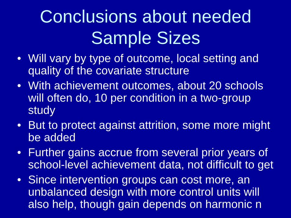
Conclusions about needed Sample Sizes
• Will vary by type of outcome, local setting and quality of the covariate structure
• With achievement outcomes, about 20 schools will often do, 10 per condition in a two-group study
• But to protect against attrition, some more might be added
• Further gains accrue from several prior years of school-level achievement data, not difficult to get
• Since intervention groups can cost more, an unbalanced design with more control units will also help, though gain depends on harmonic n
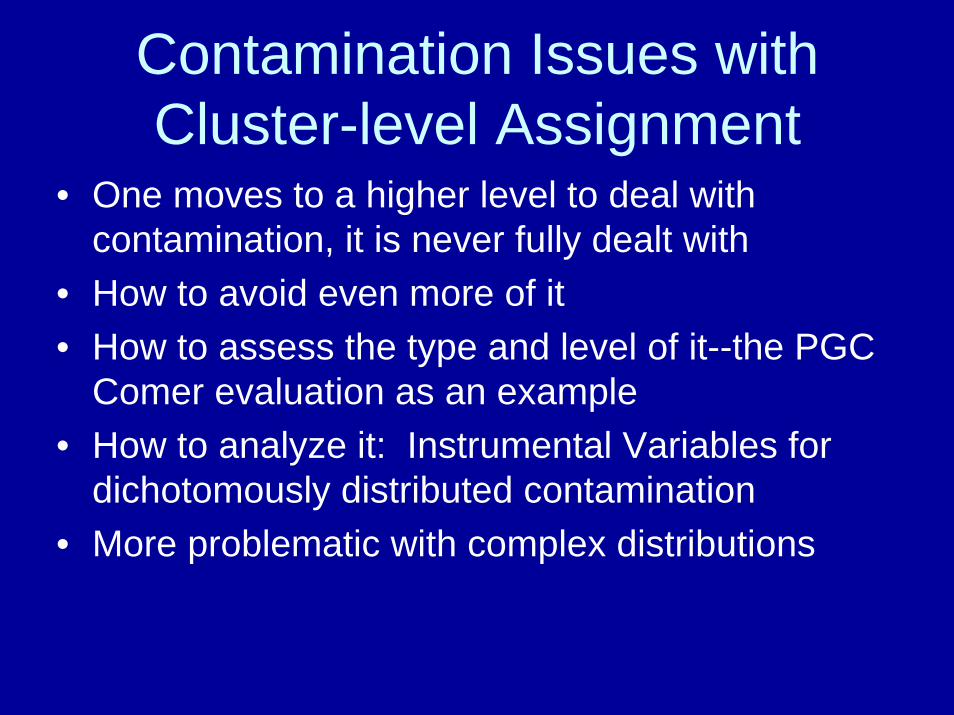
Contamination Issues with Cluster-level Assignment
• One moves to a higher level to deal with contamination, it is never fully dealt with
• How to avoid even more of it• How to assess the type and level of it--the PGC
Comer evaluation as an example• How to analyze it: Instrumental Variables for
dichotomously distributed contamination• More problematic with complex distributions

Summary re RCTs
• Best in theory and practice for cause• Assumptions, and they need to be tested• Marriage of statistical theory and an ad
hoc “theory” of implementation, as with survey research
• Not always usable in practice• Least usable when….

Summary 2
• Lower level at which assign the better• Higher order designs can be expensive• Crucial role of covariates in reducing sample
size requirements at higher level• Crucial role of pretest among these covariates• Crucial role of description of implementation
based on program theory and quality measurement of key aspects
• Black box RCTs not a good idea in education

Remember, though…• Explanation requires that X causes Y,• Quantitative causal models test model fit and not
each of the individual causal links postulated in them
• Knowledge of these links is largely outside of the model and the data testing its overall fit
• So, the activity theory is an essential component of all explanatory theories.
• It identifies “the cement of the universe”, though not all the building blocks making up the universe