quasi-central bank regimes and the quantity of money … quasi ‐ central bank regimes and the...

1

Quasi‐Central Bank

Regimes

and

the

Quantity Theory

of

Money (QTM): Zooming

Monetary

Anomalies

in Argentina 1870‐2010

Guillermo Bozzoli (DIW Berlin and Universidad Torcuato Di Tella)*

Gerardo della Paolera (GDN and Universidad de San Andres)*

November

2012

Presentation

for

the

Session

“Lessons

on

Monetary

Institutions‐Saturday

3rd November

2012 LACEA‐LAMES 2012‐Lima , Peru

2

The

Central Problem: Argentina could

not Conquer

Inflation

•

A systematic

study

of

the

Argentine

monetary, fiscal and

financial

history

is

a phenomenon

of

recent

but

growing

interest.

•

After

the

1980s, numerous

scholars

addressed

the

subject

of

why

this

once promising

country failed

to

support

stable

monetary, fiscal and

financial

policies.

•

But

there

was

one

pioneer

scholar

above

them

all: Roberto

Cortes Conde

•

A pioneer

in the

quantitative

monetary

history

of

Argentina

•

Dinero, Deuda y Crisis: Evolución fiscal y Monetaria en la

Argentina (1989)

4

On

the

shoulders

of

Roberto Cortes Conde

•

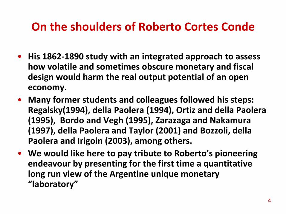
His

1862‐1890 study with an integrated approach to assess

how volatile

and

sometimes

obscure

monetary

and

fiscal

design

would

harm

the

real output potential

of

an

open

economy.•

Many

former

students

and

colleagues

followed

his

steps:

Regalsky(1994), della

Paolera

(1994), Ortiz and

della

Paolera

(1995), Bordo and

Vegh

(1995), Zarazaga

and

Nakamura

(1997), della

Paolera

and

Taylor (2001) and

Bozzoli, della

Paolera

and

Irigoin

(2003), among

others.

•

We

would

like

here

to

pay

tribute to

Roberto’s

pioneering

endeavour

by presenting

for

the

first

time a quantitative

long run

view

of

the

Argentine

unique

monetary

“laboratory”

5

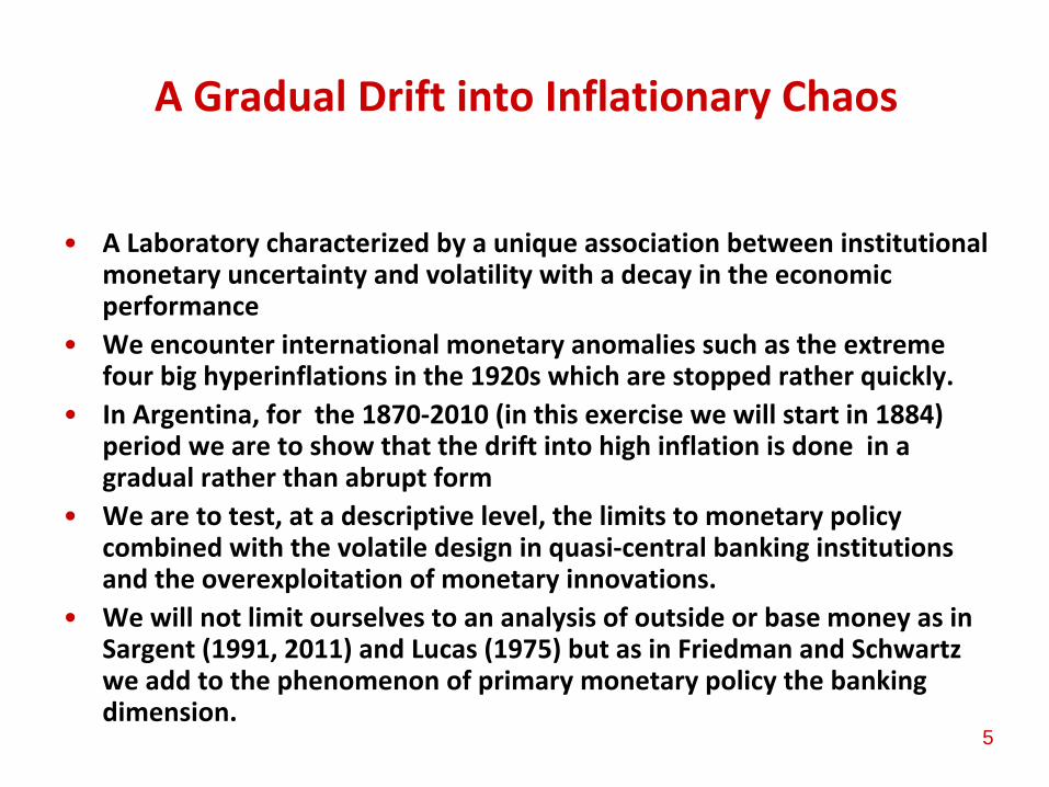
A Gradual Drift

into

Inflationary

Chaos

•

A Laboratory

characterized

by a unique

association

between

institutional

monetary

uncertainty

and

volatility

with

a decay

in the

economic

performance

•

We

encounter

international

monetary

anomalies

such

as the

extreme

four

big

hyperinflations

in the

1920s which

are stopped

rather

quickly.•

In Argentina, for

the

1870‐2010 (in this

exercise

we

will

start

in 1884)

period

we

are to

show that

the

drift

into

high

inflation

is

done in a

gradual rather

than

abrupt

form•

We

are to

test, at a descriptive

level, the

limits

to

monetary

policy

combined

with

the

volatile

design

in quasi‐central banking

institutions

and

the

overexploitation

of

monetary

innovations.•

We

will

not

limit

ourselves

to

an

analysis

of

outside

or

base money

as in

Sargent

(1991, 2011) and

Lucas (1975) but

as in Friedman and

Schwartz

we

add

to

the

phenomenon

of

primary

monetary

policy

the

banking

dimension.

6

The

Outline

of

the

Presentation

•

By presenting

an

1884‐2010 continuous

annual

time series

of

several

key

macrovariables we

discuss

the

long run

view

of

the

Argentine

Monetary

History

•

We

address

then

the

periodization

matching

each

period

with

the

monetary

and

quasi‐central banking

policies, the

institutional

innovations

and

the

economic

outcomes.

•

Then

we

briefly

zoom the

major

monetary

and

financial

anomalies

to

assess

which

macro‐variables produce “jumps”

following

crises

or

failed

institutional

or

unsustainable

policy

paths.•

Finally, we

run

a rough

exercise

of

testing

the

QTM which

acts

as a preliminary

corollary

of

the

study

to

assess

when

the

theory

holds

and

when

it

breaks down.

7

A Long Run View: the

Secular Evolution

of Some

Key

Macro Variables

•

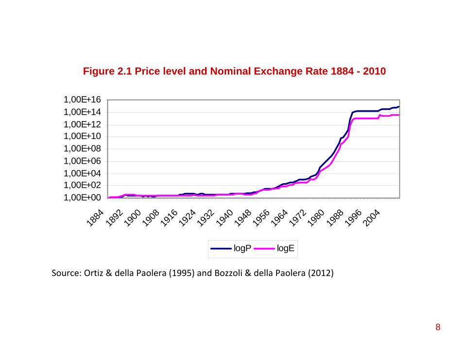
Prices

and

Exchange Rates

•

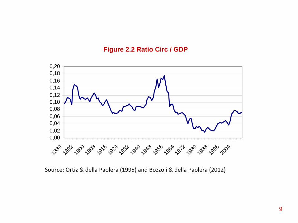
Currency

in hands

of

the

Public

as a proportion

of

Output

•

The

annual

change

in the

log

Currency

in hands

of

the

Public

•

Velocity

in its

three

definitions

: Currency, Money Base M0,

Money Supply

M3

•

Money Multiplier

M3 as a ratio of

M0

•

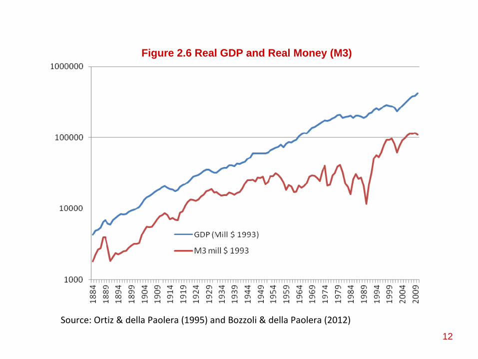
Secular evolution

of

Real Output (GDP) and

Real Money M3

•

Detrended

Log real GDP and

log

real M3

8

1,00E+001,00E+021,00E+041,00E+061,00E+081,00E+101,00E+121,00E+141,00E+16

1884

1892

1900

1908

1916

1924

1932

1940

1948

1956

1964

1972

1980

1988

1996

2004

logP logE

Source: Ortiz & della Paolera (1995) and Bozzoli & della Paolera (2012)

Figure 2.1 Price level and Nominal Exchange Rate 1884 - 2010

9

0,000,020,040,060,080,100,120,140,160,180,20

1884

1892

1900

1908

1916

1924

1932

1940

1948

1956

1964

1972

1980

1988

1996

2004


Figure 2.2 Ratio Circ / GDP

10

010203040506070

1884

1892

1900

1908

1916

1924

1932

1940

1948

1956

1964

1972

1980

1988

1996

2004

V circ V M0 V M3


Figure 2.4 Velocity in its three definitions

11

0,00

1,00

2,00

3,00

4,00

5,00

6,00

7,00

1884

1892

1900

1908

1916

1924

1932

1940

1948

1956

1964

1972

1980

1988

1996

2004


Figure 2.5 Money multiplier M3 / M0

12

Figure 2.6 Real GDP and Real Money (M3)


13

Figure 2.7 Detrended Log real GDP and log real M3


14

Table 1. Evolution of Key Macroeconomic Variables

1884 ‐ 1934 1934 ‐ 1945 1945 ‐ 1977 1977 ‐ 2010 1884 ‐ 1944 1944 ‐ 2010Average % Change

M3 (ctes) 7,6 8,9 48,9 230,9 8,0 139,8M0 (ctes) 6,1 13,6 51,8 215,3 7,7 133,2M3 ‐ M0 9,8 6,8 47,9 329,8 9,3 190,1

P (2004= 1000000) 3,4 6,0 50,9 280,5 3,7 167,6E 3,5 2,2 42,4 262,9 3,0 155,7

GDP (real end year) 4,6 3,7 4,2 2,7 4,4 3,4

Average level

M3/M0 2,30 2,60 1,90 3,10 2,34 2,52M3/circ 4,32 4,54 3,10 5,22 4,34 4,15

(M0 ‐ circ) / M3 0,21 0,17 0,20 0,22 0,21 0,07circ/M3 0,10 0,09 0,10 0,04 0,10 0,07V. circ 10,35 10,85 13,53 29,28 10,40 21,28V. M0 5,56 6,24 8,33 15,29 5,64 11,86V.M3 2,55 2,39 4,23 5,87 2,52 3,42

M3 St. Dev. 0,52 0,21 1,77 3,25 0,48 5,26


15

Monetary

Institutions

and

Regimes

•

In Table

2, we

have

characterized

the

institutional

setting

for

11 macro‐periods

and

the

average annual

inflation

rate

for

each

of

them

is

shown.

•

The

institutional

domains

characterized

are: (1) type

of

monetary

authority

(ie

Currency

board, Central Bank; Plural

Banks of

Issue); Lender

of

last

resort

function

or

not;

Monetary

Regime; Exchange Rate

regime; Existence

of

a

specific

banking

Law; Fractional

Reserve banking

system.

•

As a synthetic

we

can observe at least, and

we

are saying

at

least, 9 different

fundamentally

different

frameworks

for

quasi‐central and

central banking

design

and

16 different

monetary

and

exchange

rate

regimes. We

are at present

identifying

more closely

banking

reforms.

16

Table 2. Monetary institutions and regimes

Period Characterization Avg. Infaltion(%)Plurality of Banks of Issue; No lender of last resortShort lived Gold Standard and Inconvertible Paper CurrencyDe facto Floating Exchange Rate paper Peso-Gold pesoAbsence of a specific Banking Law and fractional-reserve banking systemMonopoly of Issue; Currency Board, No lender of last resortInconvertible CurrencyFree Floating Exchange rate Paper Peso-Gold pesoAbsence of a specific Banking Law and fractional-reserve banking systemCurrency Board; No lender of last resortFull-Fledge Gold StandardFixed Exchange RateAbsence of Banking Law and fractional reserve banking systemCurrency Board; Rediscount and Sterilization-prone laws in 1914

One way Gold Standard; gold withdrawals from currency board prohibitedFloating Exchange Rate paper peso-Gold peso,short lived GSAbsence of Banking Law and fractional Reserve banking systemCurrency Board switch to a Fiduciary RegimeDepreciaition of the Paper-PesoExchange Rate ControlsPolicies of Lender of last Resort

0,6

1884-1891 17,0

2,0

1,7

1,6

1891-1899

1899-1914

1914-30

1930-34

17

Period Characterization Avg. Infaltion(%)Full Fledge Central BankCreation of a Bad-Bank to clean financial systemLender of last resortOpen Market Operations and steril ization policiesMultiple Exchange RatesCentral BankNationalization of Deposits and Directed allocation of CreditRegulated interest rate. Multiple exchange ratesCentral BankFractional Banking System (with brief Nationalization of deposits 1973-77)Regulated interest ratesDifferent exchange rate regimes (from multiple type system to managed floating)Central Bank with fractional banking system.Interest rates are set by the banks freely, then regulated after the Banking-Debt Crisis of 1981-82High inflation rates with Hyperinflation in 1989-90Deposits are frozen and converted into bonds (Bonex89)Tendency to set multiple exchange ratesConvertibility period Central Bank can no longer finance fiscal imbalances Inflation rates converge to U.S. levelsPost-Convertibility periodManaged floating with initial overshooting and confiscation of depositsReduction in the degree of autonomy of the Central BankInflation rates diverge from U.S. levels

Source: Ortiz & Della Paolera (1995) and Bozzoli & Della Paolera (2012)

2001-2010

1957-1977

1977-1991

8,1

17,4

622,8

69,5

6,0

1991-2001

18,91945-1957

1934-1945

18

Periodization

and

Analysis

of

Monetary

Policy and

Institutional

Innovations

•

The

pre‐Central Bank

period

1884‐1934 with

5 sub‐periods: (1) Baring

period

1884‐1891; (2) A search

to

resume gold standard

91‐99; (3) 99‐

1914 Full‐fledged

Gold Standard period; (4) 14‐30 Struggling

with

the

Monetary

Regime; (5) 1930‐1934 From

a metallic

to

a fiduciary

regime.

•

The

Creation

of

the

Central Bank

and

its

first

10 years

in operation: 1935‐

1945.

•

Drifting

Towards

Inflation

or

When

Inflation

Conquered

Argentina, 1945‐

2010 with

5 sub‐periods: (1) 1945‐1957 Central Bank

and

financial

system

nationalization; (2) 57‐77 Full‐Fledge

Central Bank

and

interest

rate

control; (3) 1977‐1991 Financial

Liberalization

and

drift

towards

hyperinflation; (4) 1991‐2001 Convertibility

Period; (5) 2001‐2010

Reduction of autonomy of Central bank

drifting

back to

inflation.

19

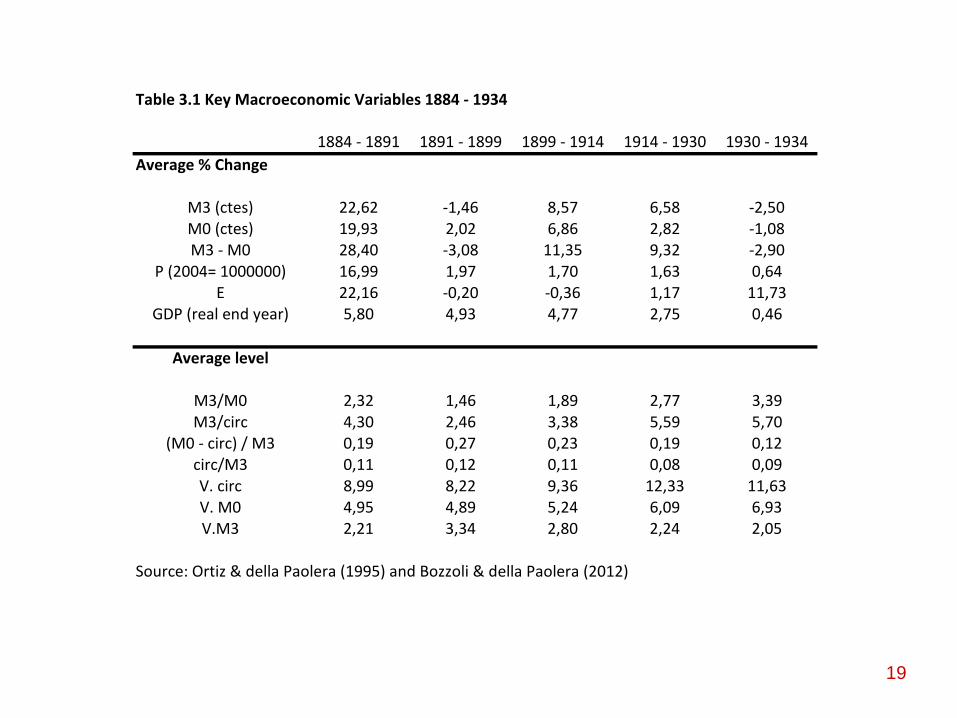
Table 3.1 Key Macroeconomic Variables 1884 ‐ 1934

1884 ‐ 1891 1891 ‐ 1899 1899 ‐ 1914 1914 ‐ 1930 1930 ‐ 1934Average % Change

M3 (ctes) 22,62 ‐1,46 8,57 6,58 ‐2,50M0 (ctes) 19,93 2,02 6,86 2,82 ‐1,08M3 ‐ M0 28,40 ‐3,08 11,35 9,32 ‐2,90

P (2004= 1000000) 16,99 1,97 1,70 1,63 0,64E 22,16 ‐0,20 ‐0,36 1,17 11,73

GDP (real end year) 5,80 4,93 4,77 2,75 0,46

Average level

M3/M0 2,32 1,46 1,89 2,77 3,39M3/circ 4,30 2,46 3,38 5,59 5,70

(M0 ‐ circ) / M3 0,19 0,27 0,23 0,19 0,12circ/M3 0,11 0,12 0,11 0,08 0,09V. circ 8,99 8,22 9,36 12,33 11,63V. M0 4,95 4,89 5,24 6,09 6,93V.M3 2,21 3,34 2,80 2,24 2,05


20

Prices and exchange rates 1884 - 1934

0123456

1884

1888

1892

1896

1900

1904

1908

1912

1916

1920

1924

1928

1932

P E

Ratio Circ/GDP1884 - 1934

0,000,020,040,060,080,100,120,140,16

1884

1888

1892

1896

1900

1904

1908

1912

1916

1920

1924

1928

1932

Velocity in its three definitions1884 - 1934

0,002,004,006,008,00

10,0012,0014,0016,00

1884

1888

1892

1896

1900

1904

1908

1912

1916

1920

1924

1928

1932

V circ V M0 V M3

Money multiplier: M3/M01884 - 1934

0,000,501,001,502,002,503,003,504,00

1884

1888

1892

1896

1900

1904

1908

1912

1916

1920

1924

1928

1932


Panel 1: 1884 - 1934

21

Chosen

Stylized

Facts

for

the

1884‐1935 period•

The

1884‐1891 period

was

one

in which

the

prevalent

mentalite

was

the

doctrine of

a plurality

of

banks

of

issue, banks

that

would

respect

an

inelastic

relationship

between

specie

and

convertible notes issued. The

government

tried

to

peg

the

paper

peso to

the

gold peso but

the

fix

collapsed

in 1891: the

Baring

Crash. Depreciation

up to

250 percent;

inflation

skyrockets, restructuring

of

the

debt; demise

of

the

financial

system, destruction

of

deposits

by almost

50 percent.•

Partial

Disinflation

and

Monetary

and

financial

reforms

for

1891‐1899, by

1899 the

price

level

of

Argentina stabilized

at a 120 percent

higher

level

than

in 1884. A period

of

Monetary

Anemia. Floating

exchange

rate

regime.

•

Resumption

of

Gold Standard in 1899 at a devaluated

rate

of

2.27 paper

pesos per

gold peso (the

previous

regime stated

that

these

should

be at

par). The

regime started with zero gold backing! Bet

worked. The

longest

period

of

a hard

peg

in Argentine

monetary

history. Price

stability,

Confidence, Financial

Deepening, high

output growth. A phenomenon

of

real exchange

rate

appreciation. Full‐fledge

GS.•

1914 Financial

Crisis: A twin

crisis which

unveiled

the

institutional

weakness

of

a Currency

Board

and

the

insufficient

lending

of

last

resort

function

to

assist

a fractional

reserve system. Suspension

of

full

Convertibility.

22

Chosen

stylized

facts

for

the

1884‐1935 period

•

Reform

of

Caja de Conversion

and

Banco de la Nacion

to

allow

for

“sterilization”

and

rediscount

policies. The

1914‐1930 period

one

way

GS

with

a short‐lived

1927‐1929 GS. In spite

of

the

measures

very

mild

depreciation

pressures

and

a mentalite

of

a transitory

limitation

to

convertibility with the aim to go back to

GS. Money multiplier

increases

substantially

but

balance sheets

of

banks

worsen

substantially. 1927‐

1929 twin

crisis again

and

Argentina abandoned

definitively

the

Gold

Standard.

•

The

1929‐1934 period

is

the

switch from

a metallic

to

a fiduciary

regime,

one

of

the

most

important

institutional

experiments

to

steer

through

the

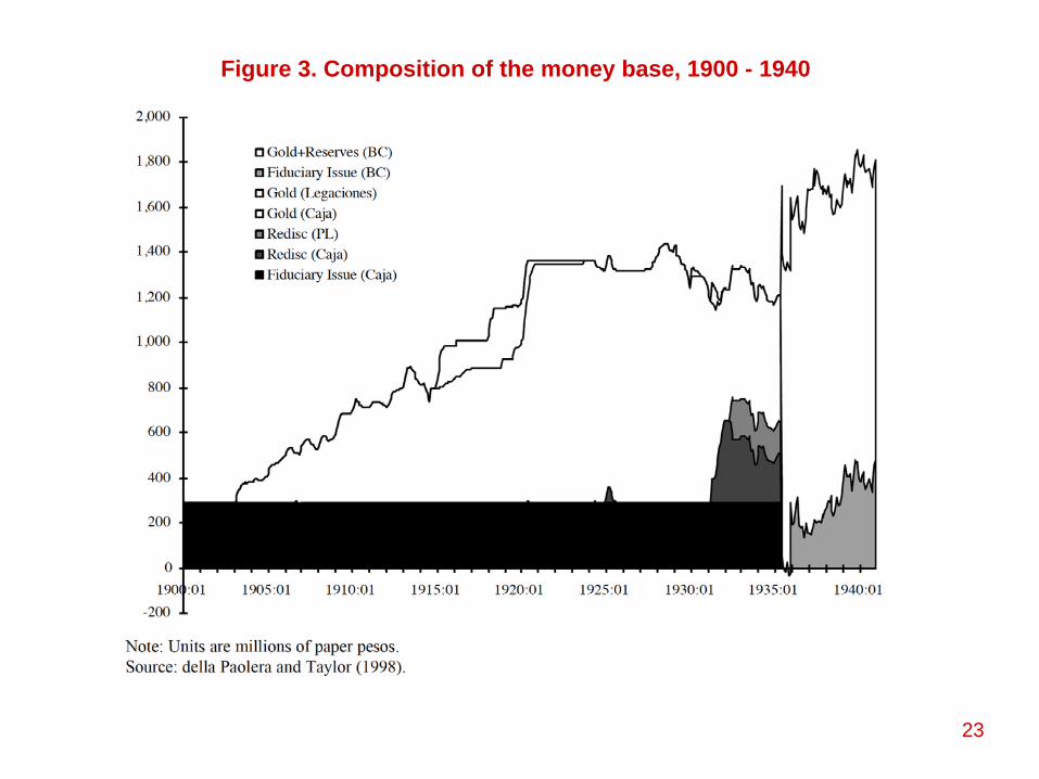
Great Depression. The

heterodox

changes

focused

on

delinking

the

monetary

expansion

(or

contraction) from

the

evolution

of

gold stocks

and

international

reserves. Backing

of

the

money

base went

from

78

percent

in 1928 to

49 percent

by 1934. Successful

insulation

from

the

Great depression; depreciation

of

paper

peso from

2.27 to

3.9 at its

peak. Financial

system

virtually

bankrupt

but

real output declines

contained.

23

Figure 3. Composition of the money base, 1900 - 1940

24

The

Central Bank

and

its

first

10 years

•

Discussion

started

in 1932. “Our

money

doctor”

Otto Niemeyer. Central Bank

(CB) created

in

1935, big

figures Raul Prebisch

and

Federico Pinedo. Measures: (1) CB take

over

currency

responsibilities

from Currency

Board; (2) CB take

responsibility

over

Exchanges

and

debt

amortizations; (3) A specific

banking

Law

and

a Supervision

and

Regulatory

Body of

financial

system

under

CB; (4) Establishment

of

a new

institution, a pioneer

concept

of

a “bad

bank”,

the

IMIB to

absorb

and

liquidate

the

nonperforming

and

junk

assets

of

the

Banco Nacion

and

private

banks; (5) to

restructure

the

Banco Nacion

and

Mortgage

National

Bank

to

limit

financing

of

the

government.•

Definitive

change

in the

monetary

regime: (1) Now

Gold and

International Reserves should

not

fall

below

25 percent

money

base (down

from

40 percent

in previous

regime); (2) Open

Market

Operations

and

rediscounts

at CB; rediscounts

should

not

surpass

10 percent

of

capital plus reserves; (3) limit

to

finance

government

to

10 percent

of

annual

government

revenues; (4) reserve requirements

established

for

the

banking

system

at 16 percent

for

sight

deposits

and

8 percent

for

savings

and

time deposits; (5) IMIB used

up 55 percent

of

the

gold revaluation

to

clean

up the

financial

system.•

Huge

potential

injection

of

liquidity

reabsorbed through

various

sterilization

mechanisms;

the

behaviour

of

the

1935‐1944 CB praised

by Triffin

(1944) as “CB of

Argentina has

developed

into

an

outstanding

institution

among

central banks

not

only

in Latin

America but

in older

countries

as well”….•

Results: money

base grew at almost

14 percent

per

annum; bank

money

contained

because

of

the

process

of

de‐leveraging; the controlled exchange rate stable after the massive

depreciation

during

the

switch regime; inflation

at 6 percent

per

annum, almost

double

than

for

the

1884‐1934 period.

25

Prices and exchange rates1934 - 1945

0,0

0,5

1,0

1,5

2,0

1934 1935 1936 1937 1938 1939 1940 1941 1942 1943 1944 1945

P E


0,000,020,040,060,080,100,120,14

1934

1935

1936

1937

1938

1939

1940

1941

1942

1943

1944

1945


0,00

5,00

10,00

15,00

1934

1935

1936

1937

1938

1939

1940

1941

1942

1943

1944

1945

V circ V M0 V M3


0,00

1,00

2,00

3,00

4,0019

3419

3519

3619

3719

3819

3919

4019

4119

4219

4319

4419

45


Panel 2: 1934 - 1945

26

Table 3.2 Key Macroeconomic Variables 1934 ‐ 2010

1934‐1945 1945‐1957 1957‐1977 1977‐1991 1991‐2001 2001‐2010Average % Change

M3 (ctes) 8,92 20,66 64,62 500,10 34,87 16,31M0 (ctes) 13,64 24,07 66,70 460,90 15,90 31,95M3 ‐ M0 6,84 18,18 65,15 724,02 50,98 12,99

P (2004= 1000000) 6,02 18,93 69,47 622,80 8,06 17,42E 2,23 21,16 54,10 578,84 8,66 25,47

GDP (real end year) 3,67 3,73 4,58 1,01 3,37 4,56

Average level

M3/M0 2,60 1,61 2,07 2,05 4,68 3,23M3/circ 4,54 2,97 3,15 5,16 5,94 4,72

(M0 ‐ circ) / M3 0,17 0,28 0,16 0,39 0,06 0,11circ/M3 0,09 0,14 0,07 0,02 0,04 0,07V. circ 10,85 7,19 17,17 41,44 25,86 16,00V. M0 6,24 3,93 10,90 16,13 19,80 10,91V.M3 2,39 2,44 5,27 8,49 4,70 3,39


27

Prices and exchange rates log 1945 - 1977

1,00E+00

1,00E+01

1,00E+02

1,00E+03

1,00E+04

1,00E+05

1945

1948

1951

1954

1957

1960

1963

1966

1969

1972

1975

logP logE


0,000,020,040,060,080,100,120,140,160,180,20

1945

1948

1951

1954

1957

1960

1963

1966

1969

1972

1975


05

10152025303540

1945

1947

1949

1951

1953

1955

1957

1959

1961

1963

1965

1967

1969

1971

1973

1975

1977

V circ V M0 V M3


0,00

0,50

1,00

1,50

2,00

2,50

3,0019

4519

4819

5119

5419

5719

6019

6319

6619

6919

7219

75


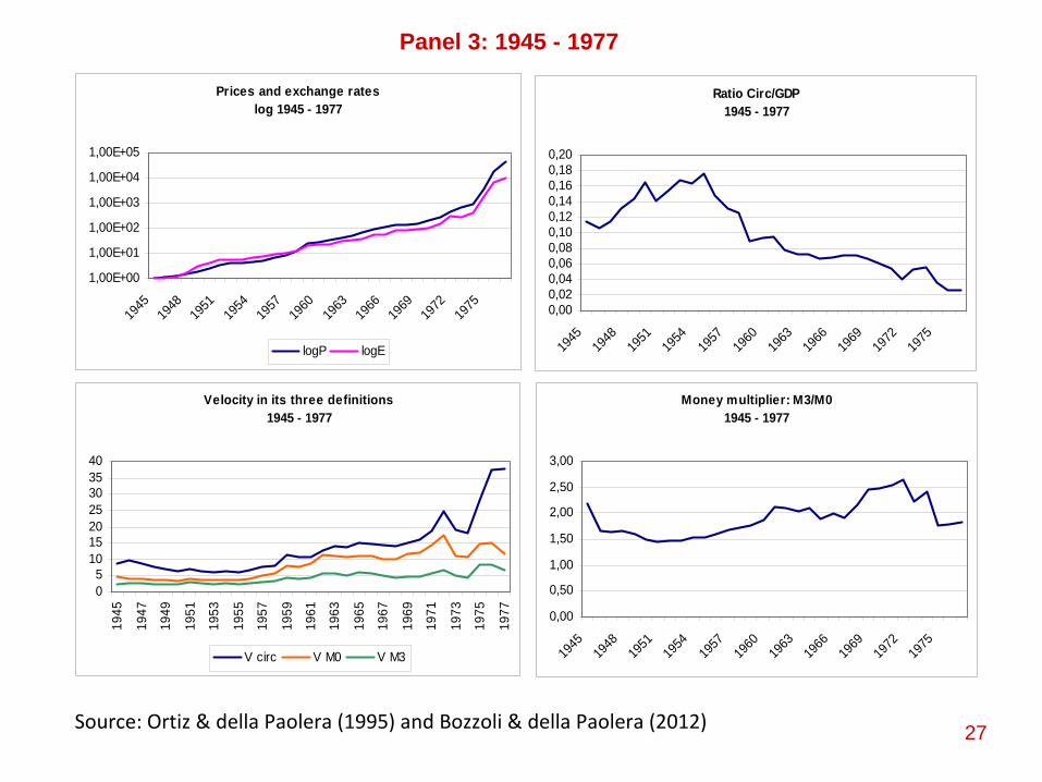
Panel 3: 1945 - 1977

28

Chosen Stylized Facts for the 1945‐1977 period

•

Drastic Reform of CB in 1946. Nationalization of CB (previously a mixed capital

institution). All appointments made by the Executive (means by Peron). Banking

operations nationalized. Direct allocation of credit and loans. Control of interest

rates. For 1945‐1957 period: Financial Repression, Inflation rates of about 20

percent per annum; 3 times more than in the first 10 years of CB

existence.

Collapse of International Reserves to 4 percent of money base.

•

New Charter of CB 1957. Again decentralized fractional reserve banking system.

However setting of max and min interest rates well below inflation rates. The

inherited imbalances in State Banks and the Social security system meant that

the economy will face chronic current account deficits (BOP crises) and persistent

fiscal deficits. Still in the 1960s the rate of growth of the economy was

satisfactory at around 4 to 4.5 percent per annum.

•

Successive stabilization programs, argentines living with chronic stop and go

policies. Devaluations averaged 50 percent per annum for the 1957‐1977 period.

Mild recovery of financial deepening judged by the evolution of the money

multiplier but velocity started to have a substantial upward trend. Until 1977,

mostly exchange Rate controls and systems of multiple exchange rate regimes

with self‐defeating results in terms of inflation control.

29

Chosen Stylized Facts for the 1945‐1977 period

•

In 1969, Political Instability and drift towards very high Inflation. The return of a direct credit

allocation measures. A clear Non‐Independent CB regime.

•

In 1973, banking system nationalized again. Substantial reduction in the money multiplier.

Inconsistencies between Price controls and nominal wage setting. The economy jumps to a path of 150

percent per annum inflation rate. By 1976, the monthly WPI inflation rate achieved a maximum of

54 percent in March 1976.

30

Prices and exchange rates log 1977 - 2010

1,00E+00

1,00E+02

1,00E+04

1,00E+06

1,00E+08

1,00E+10

1977

1980

1983

1986

1989

1992

1995

1998

2001

2004

2007

2010

logP logE


0,000,010,020,030,040,050,060,070,080,09

1977

1980

1983

1986

1989

1992

1995

1998

2001

2004

2007

2010


010203040506070

1977

1979

1981

1983

1985

1987

1989

1991

1993

1995

1997

1999

2001

2003

2005

2007

2009

V circ V M0 V M3


0

1

2

34

5

6

7

1977

1979

1981

1983

1985

1987

1989

1991

1993

1995

1997

1999

2001

2003

2005

2007

2009


Panel 4: 1977 - 2010

31

Chosen Stylised Facts for 1977‐1982 Towards Hyperinflation

•

1977‐1983 : Financial Liberalization and freeing of interest rates by

1977 with the

Ley de Entidades Financieras. The period of the Tablita: a system of pre‐

announced devaluation rates set below the previous experienced inflation rates,

a mechanism to dampen inflationary expectations. Led to an increasing degree

of domestic currency overvaluation which was unsustainable in the long‐run.

Banking Crisis in 1980, the beginning of the end of the Tablita experiment.

Melting down of the financial sector and the US shifts to a contractionary

monetary policy regime.

•

Since the financial system was semi‐dollarized, firms and the public sector had

liabilities that were dollar denominated and adjusted under a floating interest

rate scheme; the increase in the international interest rate meant the

bankruptcy of the financial system and the end of the financial deepening

experiment.

•

In 1982, CB interventions were implemented to solve the “twin”

problems of

firm’s indebtedness and bank insolvency. The “licuacion”

of liabilities started and

the Malvinas conflict added to the problems as Argentina entered

into default on

its external debt.

32

Chosen Stylized Facts for 1983‐1991

•

Democracy regained in 1983. The most ambitious plan during Alfonsin’s tenure,

the Austral Plan to curb inflation and restore investment and growth. Initial

success from an average inflation rate of 660 percent (averaging

CPI and WPI)

per annum to 70 percent in 1986. But again, wages, prices and exchange rates

were travelling inconsistent paths. CB tried to counteract the fiscal and wage

induced monetary expansion by increasing reserve requirements and absorbing

excess liquidity with a vast array of bonds.

•

The instrument that triggered the jump towards hyperinflation was the “Cuenta

de Regulacion Monetaria”

a mechanism to remunerate banking reserves which

lead to the denominated quasi‐fiscal deficits. As inflationary expectations

augmented, interest rates paid to maintain deposits in banks skyrocketed and

the CB embarked into a Ponzi type of scheme until the final run against deposits

and domestic currency occurred in 1989.

•

A short‐lived but traumatic hyperinflation occurred during the June 1989‐

March

1990. To halt hyperinflation, all short‐term debt and all term deposits were

compulsively converted into a long‐term dollar denominated bond, the BONEX

89. A default on internal debt was a very much needed mechanism to await for

still another monetary innovation: the Convertibility Plan.

33

The Convertibility Plan 1991‐2001

•

A Drastic Monetary reform in 1991: the Convertibility of the domestic currency to the

dollar. A regime of a pegged peso‐dollar standard. A 1992 Reform and full Autonomy of

the CB with the aim to “preserve the value of the currency”

and eliminate the possibility

for the CB to fund public deficits. The stopping of inflation was almost immediate. Inflation

started to converge to international levels.

•

Financial Deepening was substantial, remonetization was under way as shown by a

sizeable fall in velocity. The tequila crisis shocked the financial system and deposits

decreased by 16% in four months until April 1995 but the CB weathered the crisis by

reducing reserve requirements, using rediscounts and having access to dollar swap lines

facilitated by the IMF.

•

However, the banking system and the access of Argentina to international capital markets

was hit by three consecutive shocks: the Asian financial crisis of 1997, the Russian crisis of

1998 and the Brazilian devaluation in early 1999.

•

Growth was reduced to zero in the period 1998‐2000. Debt/GDP ratio grew and soon the

public sector started to crowd out credit from the private sector. In 2001, the government

expelled the President of the CB in April and sold bonds to banks allowing them to count

these as banking reserves starting a process of “pollution”

of bank assets. The run was

unabated until the “corralito”, a freeze in bank accounts was decreed. This meant the end

of the Convertibility and an initial devaluation of 300 percent by January 2002.

34

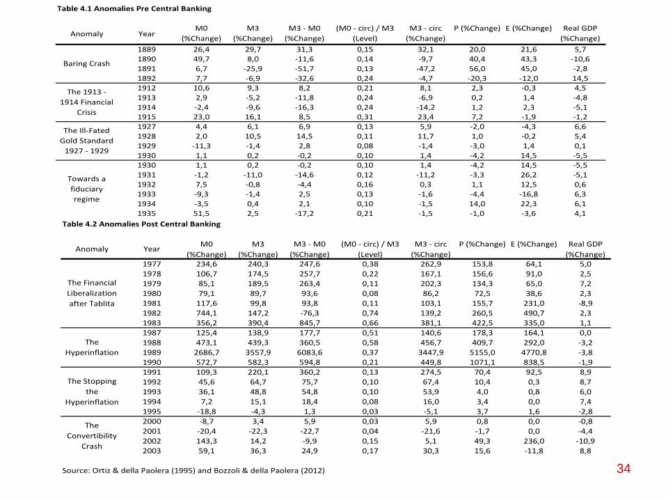
Table 4.1 Anomalies Pre Central Banking

Anomaly YearM0

(%Change)M3

(%Change)M3 ‐ M0 (%Change)

(M0 ‐ circ) / M3 (Level)

M3 ‐ circ (%Change)

P (%Change) E (%Change) Real GDP (%Change)

1889 26,4 29,7 31,3 0,15 32,1 20,0 21,6 5,71890 49,7 8,0 ‐11,6 0,14 ‐9,7 40,4 43,3 ‐10,61891 6,7 ‐25,9 ‐51,7 0,13 ‐47,2 56,0 45,0 ‐2,81892 7,7 ‐6,9 ‐32,6 0,24 ‐4,7 ‐20,3 ‐12,0 14,51912 10,6 9,3 8,2 0,21 8,1 2,3 ‐0,3 4,51913 2,9 ‐5,2 ‐11,8 0,24 ‐6,9 0,2 1,4 ‐4,81914 ‐2,4 ‐9,6 ‐16,3 0,24 ‐14,2 1,2 2,3 ‐5,11915 23,0 16,1 8,5 0,31 23,4 7,2 ‐1,9 ‐1,21927 4,4 6,1 6,9 0,13 5,9 ‐2,0 ‐4,3 6,61928 2,0 10,5 14,5 0,11 11,7 1,0 ‐0,2 5,41929 ‐11,3 ‐1,4 2,8 0,08 ‐1,4 ‐3,0 1,4 0,11930 1,1 0,2 ‐0,2 0,10 1,4 ‐4,2 14,5 ‐5,51930 1,1 0,2 ‐0,2 0,10 1,4 ‐4,2 14,5 ‐5,51931 ‐1,2 ‐11,0 ‐14,6 0,12 ‐11,2 ‐3,3 26,2 ‐5,11932 7,5 ‐0,8 ‐4,4 0,16 0,3 1,1 12,5 0,61933 ‐9,3 ‐1,4 2,5 0,13 ‐1,6 ‐4,4 ‐16,8 6,31934 ‐3,5 0,4 2,1 0,10 ‐1,5 14,0 22,3 6,11935 51,5 2,5 ‐17,2 0,21 ‐1,5 ‐1,0 ‐3,6 4,1

Baring Crash

The 1913 ‐ 1914 Financial

Crisis

The Ill‐Fated Gold Standard 1927 ‐ 1929

Towards a fiduciary regime

Table 4.2 Anomalies Post Central Banking

Anomaly YearM0

(%Change)M3

(%Change)M3 ‐ M0 (%Change)

(M0 ‐ circ) / M3 (Level)

M3 ‐ circ (%Change)

P (%Change) E (%Change) Real GDP (%Change)

1977 234,6 240,3 247,6 0,38 262,9 153,8 64,1 5,01978 106,7 174,5 257,7 0,22 167,1 156,6 91,0 2,51979 85,1 189,5 263,4 0,11 202,3 134,3 65,0 7,21980 79,1 89,7 93,6 0,08 86,2 72,5 38,6 2,31981 117,6 99,8 93,8 0,11 103,1 155,7 231,0 ‐8,91982 744,1 147,2 ‐76,3 0,74 139,2 260,5 490,7 2,31983 356,2 390,4 845,7 0,66 381,1 422,5 335,0 1,11987 125,4 138,9 177,7 0,51 140,6 178,3 164,1 0,01988 473,1 439,3 360,5 0,58 456,7 409,7 292,0 ‐3,21989 2686,7 3557,9 6083,6 0,37 3447,9 5155,0 4770,8 ‐3,81990 572,7 582,3 594,8 0,21 449,8 1071,1 838,5 ‐1,91991 109,3 220,1 360,2 0,13 274,5 70,4 92,5 8,91992 45,6 64,7 75,7 0,10 67,4 10,4 0,3 8,71993 36,1 48,8 54,8 0,10 53,9 4,0 0,8 6,01994 7,2 15,1 18,4 0,08 16,0 3,4 0,0 7,41995 ‐18,8 ‐4,3 1,3 0,03 ‐5,1 3,7 1,6 ‐2,82000 ‐8,7 3,4 5,9 0,03 5,9 0,8 0,0 ‐0,82001 ‐20,4 ‐22,3 ‐22,7 0,04 ‐21,6 ‐1,7 0,0 ‐4,42002 143,3 14,2 ‐9,9 0,15 5,1 49,3 236,0 ‐10,92003 59,1 36,3 24,9 0,17 30,3 15,6 ‐11,8 8,8


The Hyperinflation

The Stopping the

Hyperinflation

The Convertibility

Crash

The Financial Liberalization after Tablita

35

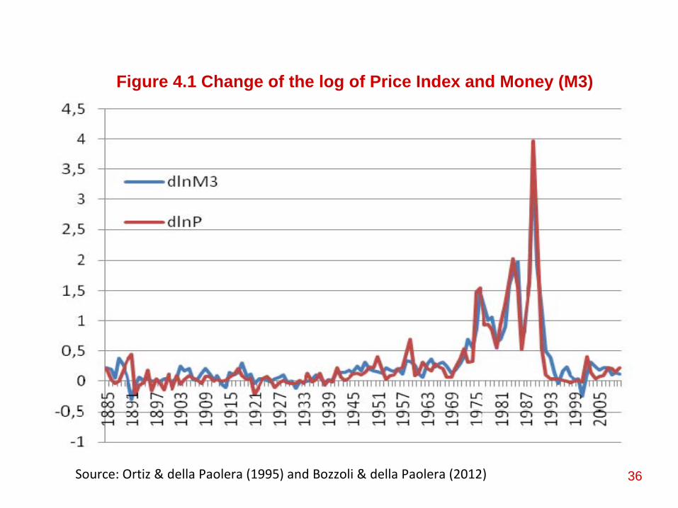
The Link Between Money and Inflation: the Quantity Theory of Money

•

In short, Argentina represents a unique laboratory in which to test the link between money and

inflation.

•

But the link could be affected by the recurrent change in monetary policies and regimes

•

In Figure 4.1 , the “nominal acceleration”

after 1945 suggests a close relation between money and

prices.

36

Figure 4.1 Change of the log of Price Index and Money (M3)


37

Linking Inflation and Money Expansion: The Equation of Exchange

•

Figure 4.2 shows the fit of inflation vs money expansion for the period 1884‐2010

•

Instead of doing moving averages to reduce “noise” in the series (as in Lucas 1980) we use the annual

values of prices and money.

•

The slope of the graph is near one, stunning result given that we use annual data.

38

Figure 4.2 Inflation vs. Money Expansion (1884 – 2010)


β = 1.02R2 = 0.87

39

Different Regimes, Different Slopes?

•

Regardless of how convincing is the result for the 1884‐2010

period, one could expect different slopes in different

monetary regimes.•

During a Gold Standard Regime we do not expect a

systematic relationship‐

for a small open economy‐

between

Money and Prices; the link between M and P is disrupted for

low inflationary biased scenarios.•

A Recent study for the US by Sargent and Surico (2011)

revisited Lucas (1980) on the relationship between moving

averages of inflation and money growth who finds for the

1953‐1977 period a unit slope. •

That prediction breaks down for 1984‐2005, under the

Volcker‐Greenspan Monetary Policy regime that strongly

reacted to inflationary shocks.

40

“For most of the last 25 years, the quantity

theory of money has been sleeping, but during the last year, unprecedented growth

in leading central banks’ balance sheets has prompted some of us to worry because

the quantity theory has slept before, only to reawaken. Our DSGE model tells us

that what puts those quantity-theoretic unit slopes to sleep is a monetary policy

rule that responds to inflationary pressure aggressively enough to prevent the

emergence of persistent movements in money growth, and that what awakens them is

a monetary policy rule that accedes to persistent movements in money growth by

responding too weakly to inflationary pressure.”

Sargent and Surico (2011, p. 110)

41

Changes in Institutions and Regimes Affect the Slope of the Relation Between Inflation and Money

•

“Tough Regimes that Adjust Money Sharply in Response to

Inflationary Pressure Results in less steep Regression than

those regimes in which monetary policy hardly counteracts

inflationary pressures.•

A period characterized by “tough responses”

or an

automatic mechanism towards “price stability”

were the

Gold Standard period of 1899‐1914(Full GS regime) and the

1914‐1930 One Way GS.•

The “discipline”

was gradually lost after 1940s when

Monetary Policy not only was too weak to counteract

inflationary policies but became adaptive to fund chronic

fiscal imbalances.

42

What does Data say in response to the predictions we have just stated?

•

In Figure 4.3 we display the 1884‐1935 plot and the 1935‐2010 plot for two money definitions M3 and

currency in hands of the public

43Source: Ortiz & della Paolera (1995) and Bozzoli & della Paolera (2012)

44

Now, the

fit

between

inflation

and

money

growth

is poor

however

prices

seem

to

be more closely

linked

to

currency

than

to

M3.

•

In sum, the

evidence

suggests

a “

breakdown”

of

the

QTM

Theory

in periods of regimes that reverse towards

price

stability

while

the

Relationship

between

Inflation

and

Money Expansion

“Awakens”

in an

inflationary

period.

•

After

all, unfortunately

Inflation

Conquered

Argentina as

shown

by our

robust

study; a fact

that

was

only

transitorily

halted

by the

ill‐fated

Convertibility

Regime of

1991.

•

Argentine

Monetary

History

Demonstrates

That

Prosperity

in Incomes

and

“Prosperity”

in Institutions

are two

very

different

things. Most

importantly, a failure

in the

second

can result

in “a melting down process” of the first

quasi-central bank regimes and the quantity of money … quasi ‐ central bank regimes and the...

Documents