Qc

A

gef1ldSmAad

g©

GEOPHYSICS, VOL. 73, NO. 3 �MAY-JUNE 2008�; P. F105–F113, 9 FIGS.10.1190/1.2895521

uasi-3D modeling of airborne TEM data by spatiallyonstrained inversion

ndrea Viezzoli1, Anders Vest Christiansen1, Esben Auken1, and Kurt Sørensen1

tsw

tftcset��m1

eHltiprr

taodoms

mgdf

ed 18 Dark. E-

ABSTRACT

We present a new methodology, spatially constrained in-version �SCI�, that produces quasi-3D conductivity modelingof electromagnetic �EM� data using a 1D forward solution.Spatial constraints are set between the model parameters ofnearest neighboring soundings. Data sets, models, and spatialconstraints are inverted as one system. The constraints arebuilt using Delaunay triangulation, which ensures automaticadaptation to data density variations. Model parameter infor-mation migrates horizontally through spatial constraints, in-creasing the resolution of layers that would be poorly re-solved locally. SCI produces laterally smooth results withsharp layer boundaries that respect the 3D geological varia-tions of sedimentary settings. SCI also suppresses the elon-gated artifacts commonly seen in interpretation results ofprofile-oriented data sets. In this study, SCI is applied to air-borne time-domain EM data, but it can also be implementedwith other ground-based or airborne data types.

INTRODUCTION

Airborne electromagnetic �AEM� surveys conducted around thelobe produce hundreds of thousands of line-kilometers of data ev-ry year. Because of the enormous computational costs involved in aull nonlinear 3D inversion, these data are usually inverted using aD forward model. The 1D model assumption is legitimate in quasi-ayered sedimentary areas, where it produces results only slightlyistorted by 2D or 3D effects �Newman et al., 1987; Sengpiel andiemon, 2000; Auken et al., 2005a�. In some cases, the resultingodels are stitched together �Macnae and Lamontagne, 1987;uken et al., 2003; Huang and Fraser, 2003�, often resulting in

brupt variations in neighboring models because of inherently noisyata and model equivalence. This is a nonoptimal result for sedimen-

Manuscript received by the Editor 24 May 2007; revised manuscript receiv1University of Aarhus, Department of Earth Sciences, Aarhus, Denm

eo.au.dk; kurt.sorensen@geo.au.dk.2008 Society of Exploration Geophysicists.All rights reserved.

F105

ary environments where the lateral variations are expected to bemooth. Models with smooth lateral variations can be achieved byorking in either the data domain or the model domain.The first approach, which is widely used with both frequency- and

ime-domain airborne EM data, entails smoothing the raw data be-ore inversion. In this case, the signal-to-noise ratio is increased athe cost of decreasing lateral resolution. In the second approach, theonstraints are applied between adjacent models during the inver-ions and the data require less smoothing, thus keeping the detailedarth information in the data. Examples of inversion methodologieshat constrain the models are the laterally constrained inversionLCI� of galvanic �Auken and Christiansen, 2004� and EM dataSantos, 2004; Auken et al., 2005b; Mansoor et al., 2006� and the si-ultaneous inversion method of galvanic data �Gyulai and Ormos,

999�.Each of these processing or inversion techniques is profile orient-

d, in the sense that they aim at producing a continuum along a line.owever, they do not create any connection between neighboring

ines. Features that are perpendicular to flight lines benefit only par-ially from inline constraints or smoothing because no informationn the model space is passed between adjacent lines. This means thatrofile-oriented techniques favor structures following the flight di-ection. Producing spatial maps based on such methodologies oftenesults in some lineation following the flight paths.

In this paper, we expand the concept of along-profile LCI to spa-ially constrained inversion �SCI�, which operates both along andcross profiles. The principles of SCI are similar to those of LCI, thenly difference being in the constraints, which are set laterally in twoimensions rather than just laterally along the flight line. Being anverdetermined problem, a full sensitivity analysis of the outputodels is produced, allowing a quantitative evaluation of the inver-

ion results.SCI has some similarity with the quasi-3D layered inversionethodology presented by Brodie and Sambridge �2006�. Their al-

orithm is specially designed for helicopter electromagnetic �HEM�ata. By using bicubic B-splines, they invert a 3D grid �using a 1Dorward solution� for a combination of layered-earth parameters and

ecember 2007; published online 11April 2008.mail: andrea.viezzoli@geo.au.dk; anders.vest@geo.au.dk; esben.auken@

gdetcw

rtpg

tlcitpiastt

atctsb

ipi

wg�sbn

p

f

w

wutbols

eolS

wcRsw

a

o

wea

n

t

Tc

F106 Viezzoli et al.

ain-phase and bias parameters related to the calibration of the HEMata. Their solution is formulated using sparse matrix solvers, whichnable them to invert extremely large data sets without dividinghem into subsets. The grid cells are often rectangular, with signifi-antly fewer node locations than observations, as opposed to SCI,hich, as we discuss, is based on actual observation locations.In the next section, we describe the SCI concept. Then we show its

esults on a data set of airborne time-domain EM �TEM� data, both inhe form of average resistivity slices maps and of resistivity sectionrofiles. We compare the results of SCI with stitched-together sin-le-site inversions and LCI.

SCI METHODOLOGY

The mathematical formulation of the SCI method is very similaro that of the LCI method �Auken and Christiansen, 2004�. It is aeast-squares inversion of a layered earth regularized through spatialonstraints, which give smooth lateral transitions. Model parameternformation from areas with well-resolved parameters migrateshrough the constraints to help resolve areas with poorly constrainedarameters. Similarly, a priori information, used to resolve ambigu-ties and to add, for example, geologic information, can be added atny point of the profile. It then migrates through the lateral con-traints to parameters at adjacent sites. In noisy soundings, the spa-ial constraints help to resolve model parameters using the informa-ion coming from the neighboring soundings.

Lateral constraints can be applied to any model parameter. Ourpproach is to constrain layer resistivity and either layer boundaryhickness or depth. Constraints on depths are often preferred overonstraints on thickness, especially in sedimentary settings, becausehe models produced display higher horizontal continuity. Con-traints on thickness are more suitable in the presence of layer-oundary discontinuities �e.g., a fault�.

The dependence of apparent resistivity on subsurface parameterss generally described as a nonlinear differentiable forward map-ing. For data inversion, we follow the established practice of linear-zed approximation by the first term of the Taylor expansion:

dobs � eobs � G� mtrue � g�mref� , �1�

here dobs is the observed data, eobs is the error on the observed data,is the nonlinear mapping of the model to the data space, and � mtrue

mtrue � mref. The true model mtrue must be sufficiently close toome arbitrary reference model mref for the linear approximation toe valid. We choose to apply logarithmic parameters to minimizeonlinearity and impose positivity.

The Jacobian matrix G contains the partial derivatives of the map-ing:

Gab ��da

�mb�2�

or the ath datum and the bth model parameter.In short, we write

G� mtrue � � dobs � eobs, �3�

here � dobs � dobs � g�mref�.The constraints are connected to the true model as

R� m � � r � e , �4�

true r

here er is the error on the constraints, with zero as the expected val-e. The term � r � �Rmref claims identity between the parametersied by constraints in the roughening matrix R. The main differenceetween SCI and LCI is in the entries of R. In LCI, only constraintsn neighboring along-line soundings �i.e., soundings along a flightine or a profile� are included, and R contains 1 and �1 for the con-trained parameters:

R � �1 0 ¯ 0 �1 0 ¯ 0 0 0

0 1 0 ¯ 0 �1 0 ¯ 0 0

] ] ]

0 0 0 ¯ 0 1 0 ¯ 0 �1� .

�5�

In SCI, the constraints are also applied to offline soundings soach model parameter is connected to many other model parametersf the same kind �e.g., resistivity of layer 2 with resistivity of otherayer 2s from constrained soundings�. The roughening matrix forCI is

R � �N1 0 ¯ 0 �1 0 ¯ 0 �1 0 ¯ 0 0 0

0 N2 0 ¯ 0 �1 0 ¯ 0 �1 0 ¯ 0 0

] ] ]

0 0 0 ¯ 0 N j 0 ¯ 0 �1 0 ¯ 0 �1� ,

�6�

here Nj is the number of models that the jth model parameter isonstrained to. For the jth row, ����1�� � Nj. In both LCI and SCI,is sparse so that sparse operations can be applied. The variance, or

trength of the constraints, is described in the covariance matrix CR,hich has nonzero entries in the same locations of R.By joining equations 3 and 4, we can write the inversion problem

s

�G

R · � mtrue � �� dobs

� r � �eobs

er , �7�

r, more compactly,

G� · � mtrue � � d� � e�. �8�

The covariance matrix for the joint observation error e� becomes

C� � �Cobs 0=

0= CR , �9�

here Cobs refers to the observational errors eobs and CR refers to therror on the constraints er. If a priori data are present, another row isdded to equation 9.

The objective function, with ND as the number of data and NC theumber of constraints, is

Q � 1

ND � NC�„� d�TC��1� d�…� 1/2

; �10�

he objective function is minimized by

� mest � �G�TC��1G���1G�TC��1� d�. �11�

his implies that the data misfit and the model roughness �i.e., theonstraints� are minimized. In LCI, only along-line soundings are

io

HzewfTs

lDis

sctsncc

vass

St

crda

3eallea1

Stntaee

idtnd

ocDrmclm

ndt3biFsMn

lartlg

ml

ssIrcw�2s

Fp

SCI for quasi-3D modeling ofAEM data F107

ncluded in the objective function. In SCI, the function includes alsoffline soundings.

The forward 1D calculation is based on the solutions in Ward andohmann �1988�. The transmitter is modeled by integrating hori-

ontal electric dipoles along the wire path. A low-pass filter �Effersøt al., 1999� is applied in the frequency domain, whereas transmitteraveform, instrument front-gate, and low-pass filters following the

ront gate are applied by convolution directly in the time domain.he frequency to time-domain transform is done using a cosine orine transform with digital filters.

Conceptually, there are three main steps in SCI. The first is to se-ect constraining points with Delaunay triangulation. We complete aelauney triangulation on the whole data set. For each data point, we

dentify the immediate nearest neighbors that will be used to con-train model parameters.

The second step is to perform the first inversion run on large dataubsets suitable for parallel computation. We identify subsets, hereinalled cells, that will be inverted independently. Using the Delauneyriangulation results to iteratively expand membership of cells, wetart with the nearest neighbors of a random point, add their nearesteighbors, and so on, until a fixed number of points is reached.Adja-ent cells overlap by one rank of nearest neighbors. For each cell, weomplete an independent SCI.

Finally, we preserve continuity across subsets with a second in-ersion run, repeating the inversion using the first inversion resultss starting models and/or a priori information for the second inver-ion. In the following sections, we expand upon each of these pointseparately.

electing constraining points with Delaunayriangulation

The first step for constraining soundings that cover an area is tohoose a strategy for connecting them. Such connections need to beepeatable, not arbitrary, and adapt as much as possible to the spatialistribution of the data set. In our approach, we use the Delaunay tri-ngulation for this purpose.

The Delaunay triangulation is the 2D version of the more generalD Delaunay tessellation, which has been widely applied in differ-nt areas of research as a favored method of representing surfacesnd reconstructing 3D objects. For a detailed description of De-aunay tessellation, see Aurenhammer �1991�. In geophysics, De-aunay triangulation has been applied to seismic tomography �Bohmt al., 2000�, to integrating data for reconstructing 3D objects �Xue etl., 2004�, for interpolating irregular data sets �Sambridge et al.,995�, and in parameter-searching algorithms �Sambridge, 1999�.

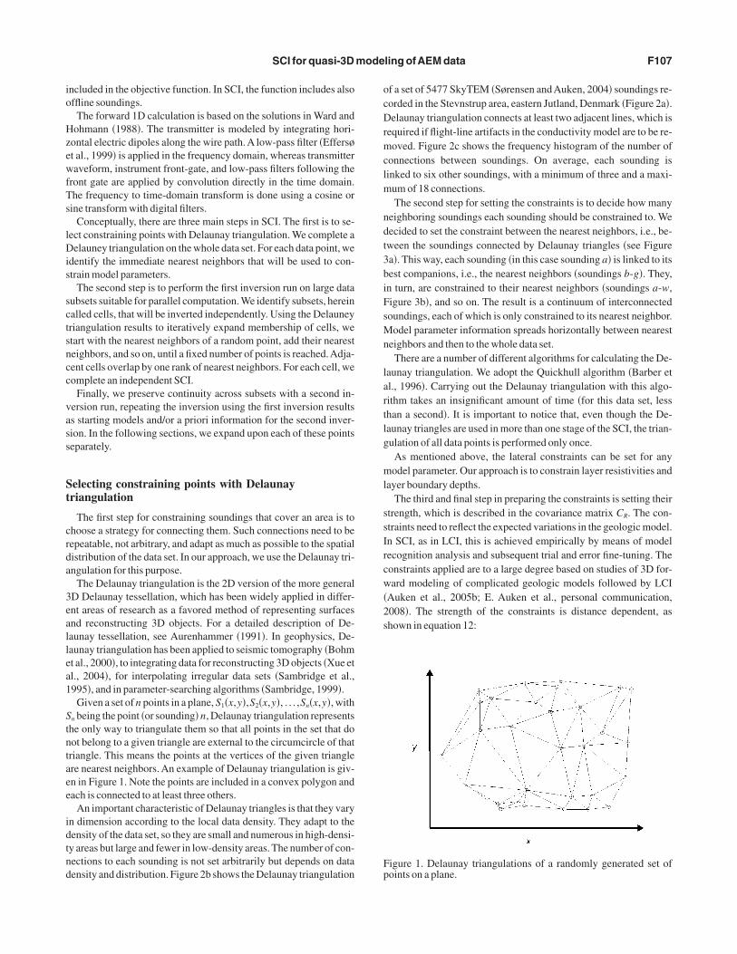
Given a set of n points in a plane, S1�x,y�,S2�x,y�, . . . ,Sn�x,y�, withn being the point �or sounding� n, Delaunay triangulation representshe only way to triangulate them so that all points in the set that doot belong to a given triangle are external to the circumcircle of thatriangle. This means the points at the vertices of the given trianglere nearest neighbors. An example of Delaunay triangulation is giv-n in Figure 1. Note the points are included in a convex polygon andach is connected to at least three others.

An important characteristic of Delaunay triangles is that they varyn dimension according to the local data density. They adapt to theensity of the data set, so they are small and numerous in high-densi-y areas but large and fewer in low-density areas. The number of con-ections to each sounding is not set arbitrarily but depends on dataensity and distribution. Figure 2b shows the Delaunay triangulation

f a set of 5477 SkyTEM �Sørensen andAuken, 2004� soundings re-orded in the Stevnstrup area, eastern Jutland, Denmark �Figure 2a�.elaunay triangulation connects at least two adjacent lines, which is

equired if flight-line artifacts in the conductivity model are to be re-oved. Figure 2c shows the frequency histogram of the number of

onnections between soundings. On average, each sounding isinked to six other soundings, with a minimum of three and a maxi-

um of 18 connections.The second step for setting the constraints is to decide how many

eighboring soundings each sounding should be constrained to. Weecided to set the constraint between the nearest neighbors, i.e., be-ween the soundings connected by Delaunay triangles �see Figurea�. This way, each sounding �in this case sounding a� is linked to itsest companions, i.e., the nearest neighbors �soundings b-g�. They,n turn, are constrained to their nearest neighbors �soundings a-w,igure 3b�, and so on. The result is a continuum of interconnectedoundings, each of which is only constrained to its nearest neighbor.

odel parameter information spreads horizontally between nearesteighbors and then to the whole data set.

There are a number of different algorithms for calculating the De-aunay triangulation. We adopt the Quickhull algorithm �Barber etl., 1996�. Carrying out the Delaunay triangulation with this algo-ithm takes an insignificant amount of time �for this data set, lesshan a second�. It is important to notice that, even though the De-aunay triangles are used in more than one stage of the SCI, the trian-ulation of all data points is performed only once.

As mentioned above, the lateral constraints can be set for anyodel parameter. Our approach is to constrain layer resistivities and

ayer boundary depths.The third and final step in preparing the constraints is setting their

trength, which is described in the covariance matrix CR. The con-traints need to reflect the expected variations in the geologic model.n SCI, as in LCI, this is achieved empirically by means of modelecognition analysis and subsequent trial and error fine-tuning. Theonstraints applied are to a large degree based on studies of 3D for-ard modeling of complicated geologic models followed by LCI

Auken et al., 2005b; E. Auken et al., personal communication,008�. The strength of the constraints is distance dependent, ashown in equation 12:

igure 1. Delaunay triangulations of a randomly generated set ofoints on a plane.

wBr

itel

os

Ps

seiietCi

aiardSi

Fltas

Fnbh

F108 Viezzoli et al.

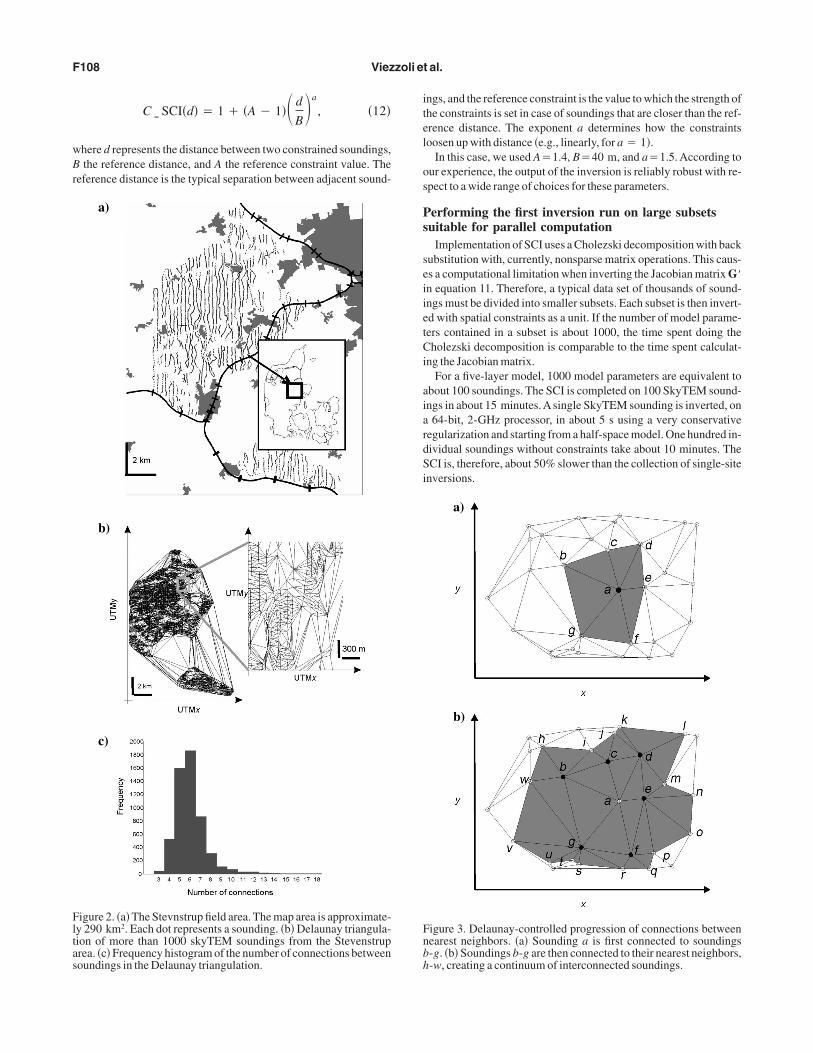
C � SCI�d� � 1 � �A � 1� d

B a

, �12�

here d represents the distance between two constrained soundings,the reference distance, and A the reference constraint value. The

eference distance is the typical separation between adjacent sound-

a)

b)

c)

igure 2. �a� The Stevnstrup field area. The map area is approximate-y 290 km2. Each dot represents a sounding. �b� Delaunay triangula-ion of more than 1000 skyTEM soundings from the Stevenstruprea. �c� Frequency histogram of the number of connections betweenoundings in the Delaunay triangulation.

ngs, and the reference constraint is the value to which the strength ofhe constraints is set in case of soundings that are closer than the ref-rence distance. The exponent a determines how the constraintsoosen up with distance �e.g., linearly, for a � 1�.

In this case, we used A�1.4, B�40 m, and a�1.5. According tour experience, the output of the inversion is reliably robust with re-pect to a wide range of choices for these parameters.

erforming the first inversion run on large subsetsuitable for parallel computation

Implementation of SCI uses a Cholezski decomposition with backubstitution with, currently, nonsparse matrix operations. This caus-s a computational limitation when inverting the Jacobian matrix G�n equation 11. Therefore, a typical data set of thousands of sound-ngs must be divided into smaller subsets. Each subset is then invert-d with spatial constraints as a unit. If the number of model parame-ers contained in a subset is about 1000, the time spent doing theholezski decomposition is comparable to the time spent calculat-

ng the Jacobian matrix.For a five-layer model, 1000 model parameters are equivalent to

bout 100 soundings. The SCI is completed on 100 SkyTEM sound-ngs in about 15 minutes.Asingle SkyTEM sounding is inverted, on64-bit, 2-GHz processor, in about 5 s using a very conservative

egularization and starting from a half-space model. One hundred in-ividual soundings without constraints take about 10 minutes. TheCI is, therefore, about 50% slower than the collection of single-site

nversions.

a)

b)

igure 3. Delaunay-controlled progression of connections betweenearest neighbors. �a� Sounding a is first connected to soundings-g. �b� Soundings b-g are then connected to their nearest neighbors,-w, creating a continuum of interconnected soundings.

eovewd

rTTtnntlw

baoods�nN

cnbaacS

iSinoptct

aSovuds

t

fopsbotp

Pi

ohmt

rawi

Fcnb

a

Fstm

SCI for quasi-3D modeling ofAEM data F109

If, for the purpose of defining the subsets, we superimpose on thentire data set predefined cells of given sizes and shapes, the densityf the soundings in such cells could vary drastically because of thearying data density of the whole data set. This would decrease CPUfficiency. Instead, we once again turn to the Delaunay triangulation,hich allows the construction of geometrically unbiased subsets ofata that adapt automatically to data-density variations.

Cell construction is a multistep process. We select a starting pointandomly and then identify its nearest neighbors, as defined above.hey produce an outer border around the staring point �Figure 3a�.hen we identify the neighbors nearest to each of the points along

he border. This way, the cell is expanded to the next order of nearesteighbors. We keep expanding the cell by selecting the nearesteighbors to the points along the border of the previous iteration un-il a predefined number of points is included in the cell. For a five-ayer model, that means approximately 100 soundings per cell,hich, including flight altitude, equates to 1000 model parameters.After the first cell C1 has been built, the second one C2 is obtained

y iterative nearest-neighbor expansions around one of the pointslong the outer border of the first cell. The third cell is built from onef the points on the outer border of either the first cell, or of the sec-nd cell, and so on, until the last cell Cq, so that each sounding in theata sets is assigned to a cell �see Figure 4a�. Each cell Cp is de-cribed by the location of the t soundings it contains: S1

p,S2p, . . . ,St

p

with t not being the same for each cell� and by the location of theearest neighbors to each of these soundings: N1

1,N21, . . . ,Nl

1;

12,N2

2, . . . ,Nm2 ; . . . ;N1

t ,N2t , . . . ,No

t .The last step, which leads to the final cells, involves expanding the

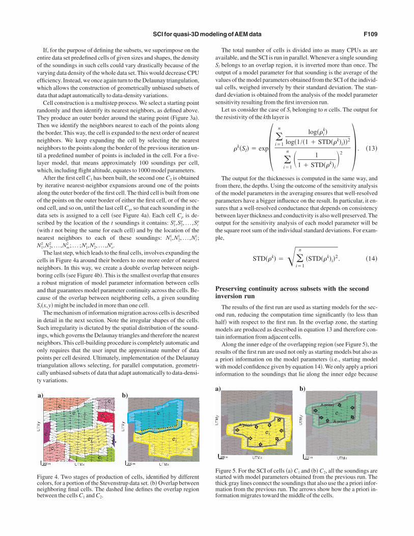
ells in Figure 4a around their borders to one more order of nearesteighbors. In this way, we create a double overlap between neigh-oring cells �see Figure 4b�. This is the smallest overlap that ensuresrobust migration of model parameter information between cells

nd that guarantees model parameter continuity across the cells. Be-ause of the overlap between neighboring cells, a given soundingl�x,y� might be included in more than one cell.The mechanism of information migration across cells is described

n detail in the next section. Note the irregular shapes of the cells.uch irregularity is dictated by the spatial distribution of the sound-

ngs, which governs the Delaunay triangles and therefore the nearesteighbors. This cell-building procedure is completely automatic andnly requires that the user input the approximate number of dataoints per cell desired. Ultimately, implementation of the Delaunayriangulation allows selecting, for parallel computation, geometri-ally unbiased subsets of data that adapt automatically to data-densi-y variations.

a) b)

igure 4. Two stages of production of cells, identified by differentolors, for a portion of the Stevenstrup data set. �b� Overlap betweeneighboring final cells. The dashed line defines the overlap region

1 2 f

The total number of cells is divided into as many CPUs as arevailable, and the SCI is run in parallel. Whenever a single soundingl belongs to an overlap region, it is inverted more than once. Theutput of a model parameter for that sounding is the average of thealues of the model parameters obtained from the SCI of the individ-al cells, weighed inversely by their standard deviation. The stan-ard deviation is obtained from the analysis of the model parameterensitivity resulting from the first inversion run.

Let us consider the case of Sl belonging to n cells. The output forhe resistivity of the kth layer is

�k�Sl� � exp� �i�1

nlog��i

k�log�1/�1 � STD��k�i��2

�i�1

n 1

1 � STD��k�i 2 � . �13�

The output for the thicknesses is computed in the same way, androm there, the depths. Using the outcome of the sensitivity analysisf the model parameters in the averaging ensures that well-resolvedarameters have a bigger influence on the result. In particular, it en-ures that a well-resolved conductance that depends on consistencyetween layer thickness and conductivity is also well preserved. Theutput for the sensitivity analysis of each model parameter will behe square root sum of the individual standard deviations. For exam-le,

STD��k� ���i�1

n

�STD��k�i�2. �14�

reserving continuity across subsets with the secondnversion run

The results of the first run are used as starting models for the sec-nd run, reducing the computation time significantly �to less thanalf� with respect to the first run. In the overlap zone, the startingodels are produced as described in equation 13 and therefore con-

ain information from adjacent cells.Along the inner edge of the overlapping region �see Figure 5�, the

esults of the first run are used not only as starting models but also aspriori information on the model parameters �i.e., starting modelith model confidence given by equation 14�. We only apply a priori

nformation to the soundings that lie along the inner edge because

) b)

igure 5. For the SCI of cells �a� C1 and �b� C2, all the soundings aretarted with model parameters obtained from the previous run. Thehick gray lines connect the soundings that also use the a priori infor-

ation from the previous run. The arrows show how the a priori in-

etween the cells C and C . ormation migrates toward the middle of the cells.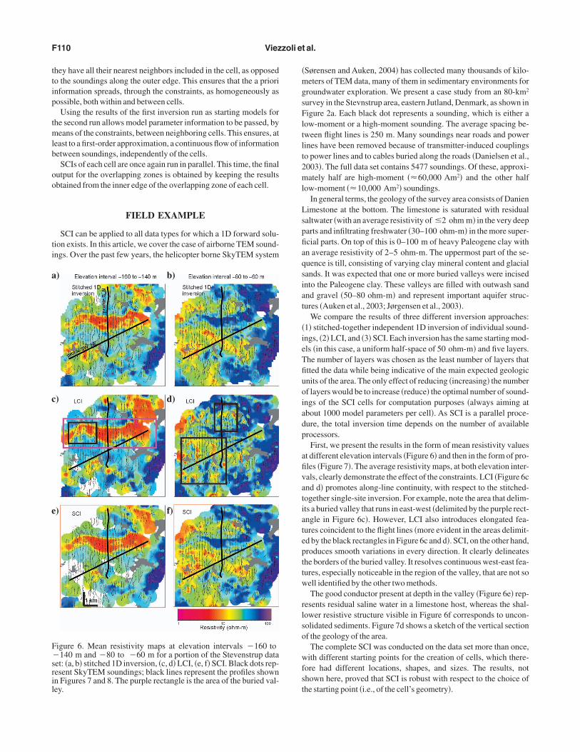

ttip

tmlb

oo

ti

�mgsFltlt2ml

Lspfiaqsiat

�ieTfiuoiadp

afivatiatepttw

rlso

wfst

a

c

e

F�sril

F110 Viezzoli et al.

hey have all their nearest neighbors included in the cell, as opposedo the soundings along the outer edge. This ensures that the a priorinformation spreads, through the constraints, as homogeneously asossible, both within and between cells.

Using the results of the first inversion run as starting models forhe second run allows model parameter information to be passed, by

eans of the constraints, between neighboring cells. This ensures, ateast to a first-order approximation, a continuous flow of informationetween soundings, independently of the cells.

SCIs of each cell are once again run in parallel. This time, the finalutput for the overlapping zones is obtained by keeping the resultsbtained from the inner edge of the overlapping zone of each cell.

FIELD EXAMPLE

SCI can be applied to all data types for which a 1D forward solu-ion exists. In this article, we cover the case of airborne TEM sound-ngs. Over the past few years, the helicopter borne SkyTEM system

) b)

) d)

) f)

igure 6. Mean resistivity maps at elevation intervals �160 to140 m and �80 to �60 m for a portion of the Stevenstrup data

et: �a, b� stitched 1D inversion, �c, d� LCI, �e, f� SCI. Black dots rep-esent SkyTEM soundings; black lines represent the profiles shownn Figures 7 and 8. The purple rectangle is the area of the buried val-ey.

Sørensen and Auken, 2004� has collected many thousands of kilo-eters of TEM data, many of them in sedimentary environments for

roundwater exploration. We present a case study from an 80-km2

urvey in the Stevnstrup area, eastern Jutland, Denmark, as shown inigure 2a. Each black dot represents a sounding, which is either a

ow-moment or a high-moment sounding. The average spacing be-ween flight lines is 250 m. Many soundings near roads and powerines have been removed because of transmitter-induced couplingso power lines and to cables buried along the roads �Danielsen et al.,003�. The full data set contains 5477 soundings. Of these, approxi-ately half are high-moment ��60,000 Am2� and the other half

ow-moment ��10,000 Am2� soundings.In general terms, the geology of the survey area consists of Danien

imestone at the bottom. The limestone is saturated with residualaltwater �with an average resistivity of �2 ohm m� in the very deeparts and infiltrating freshwater �30–100 ohm-m� in the more super-cial parts. On top of this is 0–100 m of heavy Paleogene clay withn average resistivity of 2–5 ohm-m. The uppermost part of the se-uence is till, consisting of varying clay mineral content and glacialands. It was expected that one or more buried valleys were incisednto the Paleogene clay. These valleys are filled with outwash sandnd gravel �50–80 ohm-m� and represent important aquifer struc-ures �Auken et al., 2003; Jørgensen et al., 2003�.

We compare the results of three different inversion approaches:1� stitched-together independent 1D inversion of individual sound-ngs, �2� LCI, and �3� SCI. Each inversion has the same starting mod-ls �in this case, a uniform half-space of 50 ohm-m� and five layers.he number of layers was chosen as the least number of layers thattted the data while being indicative of the main expected geologicnits of the area. The only effect of reducing �increasing� the numberf layers would be to increase �reduce� the optimal number of sound-ngs of the SCI cells for computation purposes �always aiming atbout 1000 model parameters per cell�. As SCI is a parallel proce-ure, the total inversion time depends on the number of availablerocessors.

First, we present the results in the form of mean resistivity valuest different elevation intervals �Figure 6� and then in the form of pro-les �Figure 7�. The average resistivity maps, at both elevation inter-als, clearly demonstrate the effect of the constraints. LCI �Figure 6cnd d� promotes along-line continuity, with respect to the stitched-ogether single-site inversion. For example, note the area that delim-ts a buried valley that runs in east-west �delimited by the purple rect-ngle in Figure 6c�. However, LCI also introduces elongated fea-ures coincident to the flight lines �more evident in the areas delimit-d by the black rectangles in Figure 6c and d�. SCI, on the other hand,roduces smooth variations in every direction. It clearly delineateshe borders of the buried valley. It resolves continuous west-east fea-ures, especially noticeable in the region of the valley, that are not soell identified by the other two methods.The good conductor present at depth in the valley �Figure 6e� rep-

esents residual saline water in a limestone host, whereas the shal-ower resistive structure visible in Figure 6f corresponds to uncon-olidated sediments. Figure 7d shows a sketch of the vertical sectionf the geology of the area.

The complete SCI was conducted on the data set more than once,ith different starting points for the creation of cells, which there-

ore had different locations, shapes, and sizes. The results, nothown here, proved that SCI is robust with respect to the choice ofhe starting point �i.e., of the cell’s geometry�.

orbcfltnAlrscip

ibwippmtt

cstbum

dnss�utmsat

stcttvmss

seMad

sSiedodt

css

SCI for quasi-3D modeling ofAEM data F111

Figures 7 and 8 show the cross sections of the two profiles drawnnto the maps in Figure 6. The two profiles allow comparison of theesults of the inversion methodologies along different directions. Inoth, the single-site stitched-together inversion gives the least lateralontinuity, as expected. The south-north profile in Figure 7 follows aight line and therefore also the chain of soundings constrained in

he LCI. This should produce good results, apart from possible mi-or distortions from 2D effects along the edges of the buried valley.sketch of the geological cross section inferred from available geo-

ogic models is shown in Figure 7d. Both the LCI and the SCI cor-ectly identify all of the main geologic units. The single-site inver-ion fails to delineate the boundary between clay and limestone re-orded in the proximity of the borehole, althought does define the boundary in other areas of therofile.

The minor difference between SCI and LCI isn the detection of the whole clay-limestoneoundary in the northern portion of the profile,hich SCI defines more continuously. This result

s because the constraints set in SCI allow modelarameter information to migrate across the flightath, not only along it �as in LCI�. Therefore,odel parameters are, better resolved. We will re-

urn to the parameter sensitivity analysis issue athe end of this section.

In Figure 7, black bold arrows indicate the lo-ation of the main discrepancies between the re-ults of the SCI and the other methods. In the por-ions of the profile where the limestone is overlainy a thick clay cover, its absolute resistivity val-es are underestimated. The thick clay layer alsoasks the presence of deeper residual saltwater.Figure 8 displays less continuity because the

irection of the southwest-northeast profile doesot coincide with flight lines and thus has a lowerounding density. Both SCI and LCI results agreeubstantially with the available geologic modelFigure 8d�. SCI, however, provides more contin-ous results overall, both at the boundary be-ween the shallow resistive layers of glacial sedi-

ents and clay and at depth along the clay-lime-tone boundary. Black bold arrows indicate oncegain the main differences between the SCI andhe other two methods.

So far, we have shown that SCI reveals theame overall geologic structures as LCI but thathey are significantly different in detail. SCI re-overs the actual geology of the area better, andhe pictures are much more coherent compared tohose based on profile-oriented LCI and the indi-idual soundings inversions. We now analyze theodel parameter covariance and the data-fit re-

idual to give a mathematical evaluation of the re-ults produced.

The spatial maps in Figure 9a and b show thetandard deviation factor for the resistivity of lay-r 3 for the LCI and for the SCI, respectively.oderately to well-determined parameters havestandard deviation factor less than 1.5; a stan-ard deviation factor greater than two corre-

a)

b)

c)

d)

Figure 7. Resiinversion, �b�

ponds to unresolved parameters �Auken and Christiansen, 2004�. InCI, more model parameter information is passed between sound-

ngs than in LCI. This decreases the uncertainty of the model param-ters, which benefit from the across-line constraints. The lower stan-ard deviation factor of Figure 9b suggests that a significant amountf model parameter information in the SCI has migrated across theirection of flight lines, allowing better resolution of model parame-ers.

The question arises whether the better model parameter resolutionomes at the cost of a worse fit to the data for the SCI because of themoother model space. The white and black dots in Figure 9 repre-ent, respectively, fitted and unfitted data �residual lower or higher

cross section for south-north profile: �a� stitched-together single-site� SCI, �d� sketch of geology cross section.

stivityLCI, �c

itdcrtlpir

imspeb

a

b

c

d

Fgether single-site inversion, �b� LCI, �c� SCI, �d� sketch of geology cross sec

Feti

F112 Viezzoli et al.

than one standard deviation of the stacked�dB/dt signal�. Their density shows that this isnot the case. The LCI and the SCI fit the data in96% and 95% of the total number of soundings,respectively. Therefore, we conclude the SCI de-creases the uncertainty of model parameterswhile fitting the data.

The mean resistivity slice map, the profiles, thesensitivity analysis of the model parameters, andthe analysis of the data fit prove that, overall, SCIfits the data and produces well-determined outputmodels that resemble the known geology of thearea better than stitched-together original inver-sions and also better than a profile-oriented inver-sion methodology such as LCI.

DISCUSSION AND OTHERAPPLICATIONS

The SCI concept is applicable to different geo-physical data types distributed on a plane. TheDelaunay triangulation ensures an efficient con-nection of data points with very irregular datadensity. Thus, SCI could be applied to a combina-tion of similar data sets coming from methodolo-gies with different data-sampling densities, suchas galvanic �surface or downhole� and TEM orHEM measurements. Despite the 1D forward ap-proximation, SCI can also be applied with suc-cess to geologic settings that present modest 2Dand 3D variations because the strength of the con-straints can be adjusted to reflect the geologicvariability of the area. Even though SCI is not de-signed for a single profile of data, it would be ap-plicable to it, effectively reducing to the LCImethod.

SCI has the potential to be particularly effec-tive in fixed-wing airborne EM �AEM� data.These systems, where the receiver is towed in abird behind and below the transmitter, are asym-metric and produce flight-direction-dependentasymmetries. That is, the model parameters �e.g.,average resistivity maps� obtained from process-

ng data flown along a line in one direction differ significantly fromhose obtained with data from the same line but flown in the oppositeirection �Smith and Chouteau, 2006�. Because adjacent lines typi-ally are flown in opposite directions, such asymmetries are usuallyemoved from maps by applying spatial filters, using perpendicularie lines, or interpolating reverse line-direction data from adjacentines �Smith and Chouteau, 2006�. The advantage of the SCI ap-roach is that, rather than being filtered or interpolated, informations passed across adjacent flight lines and used to increase model pa-ameter resolution.

Even when using a nonspecialized spare matrix operation such asn the present implementation, there is no inherent limit on the di-

ension of the data sets that can be inverted with SCI. Larger dataets increase the number of cells and therefore slow down the com-letion of the SCI process �or require more parallel processes�. How-ver, dividing the data set into subsets allows SCI to be applied to ar-itrarily large data sets. Applying specialized sparse matrix opera-

� stitched-to-tion.

)

)

)

)

igure 8. Resistivity cross section for the southwest-northeast profile: �a

a) b)

igure 9. Layer 3, standard deviation factor of resistivity of third lay-r in �a� LCI and �b� SCI. The white and black dots represent, respec-ively, data that were fitted or not fitted within the noise level by thenversions.

tt

inllcsotta

hdwiaa

sttUtCmtC

A

A

A

A

A

B

B

B

D

E

G

H

J

M

M

N

S

S

S

S

S

S

W

X

SCI for quasi-3D modeling ofAEM data F113

ions, the subject of ongoing work, will largely increase the size ofhe cells.

CONCLUSIONS

SCI applies horizontal constraints for ensuring lateral continuity,mproving resolution of model parameters for single stations that areot well resolved by the data from that station alone. Use of De-aunay triangulation for the constraints allows SCI to adapt efficient-y to data-density variations. In profile-oriented data sets, it ensures aonnection between adjacent lines by means of across-line con-traints. Therefore, it eliminates the common elongated features thatften coincide with the direction of the survey �i.e., flight lines� andhat distort the continuity of geologic units across flight lines. Al-hough based on a 1D forward model, SCI results in a computation-lly practical, quasi-3D inversion of EM data.

SCI can be applied to different data types. In the study presentedere, SCI was applied successfully to quasi-3D modeling of TEMata in a sedimentary environment. It produced laterally smooth,ell-determined results that are more geologically reasonable than

ndividual sounding inversions or the profile-oriented LCI. The SCIllowed a significant improvement in the mapping of the intermedi-te clay-limestone interface.

ACKNOWLEDGMENTS

The authors would like to thank the County of Aarhus for permis-ion to use the Stevnstrup data set and for numerous discussions onhe output with Sine Rasmussen and Verner Søndergaard. We alsohank Joakim Westergaard �from the hydrogeophysics group of theniversity of Aarhus�, who was partly responsible for reprocessing

he data prior to our experiments, and associate professor Nielshristensen for numerous comments and enhancements of thisanuscript. Also, comments from the reviewers greatly increased

he readability of this manuscript. This work was funded by theounty ofAarhus, County of Vejle, and HGG.

REFERENCES

uken, E., and A. V. Christiansen, 2004, Layered and laterally constrained2D inversion of resistivity data: Geophysics, 69, 752–761.

uken, E., A. V. Christiansen, B. H. Jacobsen, N. Foged, and K. I. Sørensen,2005a, Piecewise 1D laterally constrained inversion of resistivity data:Geophysical Prospecting, 53, 497–506.

uken, E., A. V. Christiansen, L. Jacobsen, and K. I. Sørensen, 2005b, Later-

ally constrained 1D inversion of 3D TEM data: Symposium on the Appli-

cation of Geophysics to Engineering and Environmental Problems �SAG-EEP� Proceedings, 519–524.

uken, E., F. Jørgensen, and K. I. Sørensen, 2003, Large-scale TEM investi-gation for groundwater: Exploration Geophysics, 33, 188–194.

urenhammer, F., 1991, Voronoi diagrams — A survey of a fundamentalgeometric data structure: ACM Computing Surveys, 23, 345–405.

arber, B., D. Dobkin, and H. Huhdanpaa, 1996, The Quickhull algorithmfor convex hulls: ACM Transactions on Mathematical Software, 22,469–483.

ohm, G., P. Galuppo, and A. Vesnaver, 2000, 3D adaptive tomography us-ing Delaunay triangles and Voronoi polygons: Geophysical Prospecting,48, 723–744.

rodie, R., and M. Sambridge, 2006, A holistic approach to inversion of fre-quency-domain airborne EM data: Geophysics, 71, no. 6, G301–G312.

anielsen, J. E., E. Auken, F. Jørgensen, V. H. Søndergaard, and K. I. Sø-rensen, 2003, The application of the transient electromagnetic method inhydrogeophysical surveys: Journal ofApplied Geophysics, 53, 181–198.

ffersø, F., E. Auken, and K. I. Sørensen, 1999, Inversion of band-limitedTEM responses: Geophysical Prospecting, 47, 551–564.

yulai, A., and T. Ormos, 1999, A new procedure for the interpretation ofVES data, 1.5-D simultaneous inversion method: Journal of Applied Geo-physics, 41, 1–17.

uang, H., and D. C. Fraser, 2003, Inversion of helicopter electromagneticdata to a magnetic conductive layered earth: Geophysics, 68, 1211–1223.

ørgensen, F., H. Lykke-Andersen, P. Sandersen, E. Auken, and E. Nørmark,2003, Geophysical investigations of buried Quaternary valleys in Den-mark: An integrated application of transient electromagnetic soundings,reflection seismic surveys and exploratory drillings: Journal of AppliedGeophysics, 53, 215–228.acnae, J., and Y. Lamontagne, 1987, Imaging quasi-layered conductivestructures by simple processing of transient electromagnetic data: Geo-physics, 52, 545–554.ansoor, N., L. Slater, F. Artigas, and E. Auken, 2006, High-resolution geo-physical characterization of shallow-water wetlands: Geophysics, 71, no.4, B101–B109.

ewman, G. A., W. L. Anderson, and G. W. Hohmann, 1987, Interpretationof transient electromagnetic soundings over three-dimensional structuresfor the central-loop configuration: Geophysical Journal of the Royal As-tronomical Society, 89, 889–914.

ambridge, M., 1999, Geophysical inversion with a neighourhood algorithm— I, Searching a parameter space: Geophysical Journal International, 138,479–494.

ambridge, M., J. Braun, and H. McQueen, 1995, Geophysical parametriza-tion and interpolation of irregular data using natural neighbours: Geophys-ical Journal International, 122, 837–857.

antos, F. A. M., 2004, 1-D laterally constrained inversion of EM34 profilingdata: Journal ofApplied Geophysics, 56, 123–134.

engpiel, K. P., and B. Siemon, 2000, Advanced inversion methods for air-borne electromagnetic exploration: Geophysics, 65, 1983–1992.

mith, R. S., and M. C. Chouteau, 2006, Combining airborne electromagnet-ic data from alternating flight directions to form a virtual symmetric array:Geophysics, 71, no. 2, G35–G41.

ørensen, K. I., and E. Auken, 2004, SkyTEM —Anew high-resolution heli-copter transient electromagnetic system: Exploration Geophysics, 35,191–199.ard, S. H., and G. W. Hohmann, 1988, Electromagnetic theory for geophys-ical applications, in M. N. Nabighian, ed., Electromagnetic methods in ap-plied geophysics: SEG, 131–311.

ue, Y., M. Sun, and A. Ma, 2004, On the reconstruction of three-dimension-al complex geological objects using Delaunay triangulation: Future Gen-

eration Computer Systems, 20, 1227–1234.