quarterly journal royal meteorological …...quarterly journal of the royal meteorological society...

Q U A R T E R L Y J O U R N A L O F T H E

R O Y A L M E T E O R O L O G I C A L S O C I E T Y

Vol. 109 OCTOBER 1983 No. 462

Quart. J . R . M e r . Soc.(1983), 109, pp. 683-717 551.509.333:551.558.21

Reduction of systematic forecast errors in the ECMWF model through the introduction of an envelope orography

By J O H N M. WALLACE*, STEFAN0 TIBALDI and ADRIAN J. SIMMONS European Centre ,/or Medium Range Weather Forecasts, Reading

(Received 6 October 1982; revised 14 April 1983)

SUMMARK Day 1 forecast errors in the ECMWF model geopotential height fields during wintertime show a distinctive

and highly reproducible signature with negative biases over the major mountain barriers. These biases are largest on days when the 500mb flow over the mountains is strong and they tend to shift position from day to day so as to remain close to the region where the jet stream crosses the mountain barrier. These systematic errors evolve through the forecast interval until by day 10 they assume an equivalent barotropic structure which strongly resembles the upper-level stationary wave pattern, but has the opposite sign, which indicates that the model does not have sufficient (presumably orographic) forcing to maintain the stationary waves.

The time evolution of the systematic error pattern is investigated by means of a series of experiments with a barotropic model, in which the observed mean wintertime 300mb flow is perturbed by a steady forcing derived from the day 1 forecast error pattern. The day 10 error patterns, as simulated by the barotropic model, bear a strong similarity to the observed ones. The forcing in the vicinity of the northern Rockies makes a particularly large contribution to the simulated day 10 error pattern whereas that in the Himalaya region appears to be relatively less important.

The impact of an enhanced orography upon the climate of the ECMWF model is investigated by carrying out a pair of extended integrations out to 50 days. The control run is based on the conventional average-type orography used for operatibnal forecasting; the other run is based on an ‘envelope orography’ constructed by adding to the conventional, grid-square averaged, orography an increment proportional to the standard deviation of the sub-grid scale variance. Results for this one, rather short pair of integrations suggest that the envelope orography may be capable of yielding a more realistic simulation of the observed wintertime flow pattern, particularly with respect to features in the Pacific and western North American sectors. Certain aspects of the zonally averaged circulation are also more realistic in this envelope simulation.

A series of 21 successive ten-day forecast integrations has also been carried out with this envelope orography from February 1982 data. Results indicate that the introduction of the envelope orography results in a slight degradation of the short-range forecasts together with a distinct improvement of the forecast beyond four days. The beneficial impact towards the end of the forecast interval appears to be large enough to increase the forecast usefulness by perhaps as much as half a day.

1. INTRODUCTION All existing numerical weather prediction models exhibit errors which are systematic

in the sense that the mean of forecast fields derived from them (taken over large numbers of forecasts for a given season and a given forecast interval) tends to be significantly different from the corresponding mean of the analyses against which the forecasts are verified. For the range of practical interest in weather forecasting, these systematic errors tend to increase with the forecast interval so that they are of greater consequence for intermediate-range (4-10-day) forecasts than they are for short-range forecasts. Assuming that a forecast model possesses a stable ‘climate’ of its own (i.e. a mean state for the

* On leave from the Department of Atmospheric Sciences, University of Washington, Seattle, Washington, USA.

683

684 J. M. WALLACE, S. TIBALDI and A. J. SIMMONS

season in question derived from one or more extended integrations in which the model is run essentially as a general circulation model), then there should presumably exist some forecast interval beyond which the systematic error ceases to grow; at this point the systematic error is equal to the difference between the model’s climate and the observed. The growth of systematic error or bias with increasing forecast interval until it reaches this limiting value is sometimes referred to as the ‘climate-drift’ problem. Experience indicates that, for the ECMWF operational model, climate drift is of primary importance in the first two or three weeks of forecast integrations, beyond that the climate of the model can be regarded as statistically stationary but for seasonal changes.

Preliminary evidence presented by Hollingsworth et at. (19801, based on an ensemble of seven forecasts, indicates that such systematic biases account for an appreciable frac- tion of the errors in medium-range forecasts. At forecast intervals of five days and beyond they are large enough to produce recognizable distortions in the planetary wave patterns in individual forecasts which, in turn, affect the steering of synoptic-scale features. Hence it would be highly desirable to reduce or, if possible, eliminate this climate drift. One possible course of action that has been considered, but rejected, would be empirically to ‘correct’ the forecast at regular intervals so as to remove the systematic component of the error. The present study was undertaken in the belief that, in the long run, the way to effect the greatest improvement in all aspects of medium-range forecasts is to use the information contained in the systematic error pattern as clues for identifying the major deficiencies in the dynamic treatments and/or physical parametrizations included in the model, and to strive to eliminate those deficiencies through modifications in the model formulation.

In the following section systematic errors in forecasts derived from the ECMWF operational model will be documented as a function of forecast interval and compared with analogous results for other forecast models and with ‘climate errors’ derived from a number of general circulation modelling experiments. For the sake of brevity, detailed results will be presented only for the extratropics of the northern hemisphere during one season: the winter of 1980/81. The section will conclude with a brief discussion of the causes of systematic error with emphasis on several pieces of evidence which suggest that an underestimation of orographic forcing, via the model lower boundary conditions, is a major contributor.

2. DOCUMENTATION OF SYSTEMATIC ERROR FOR THE 1980/81 WINTER

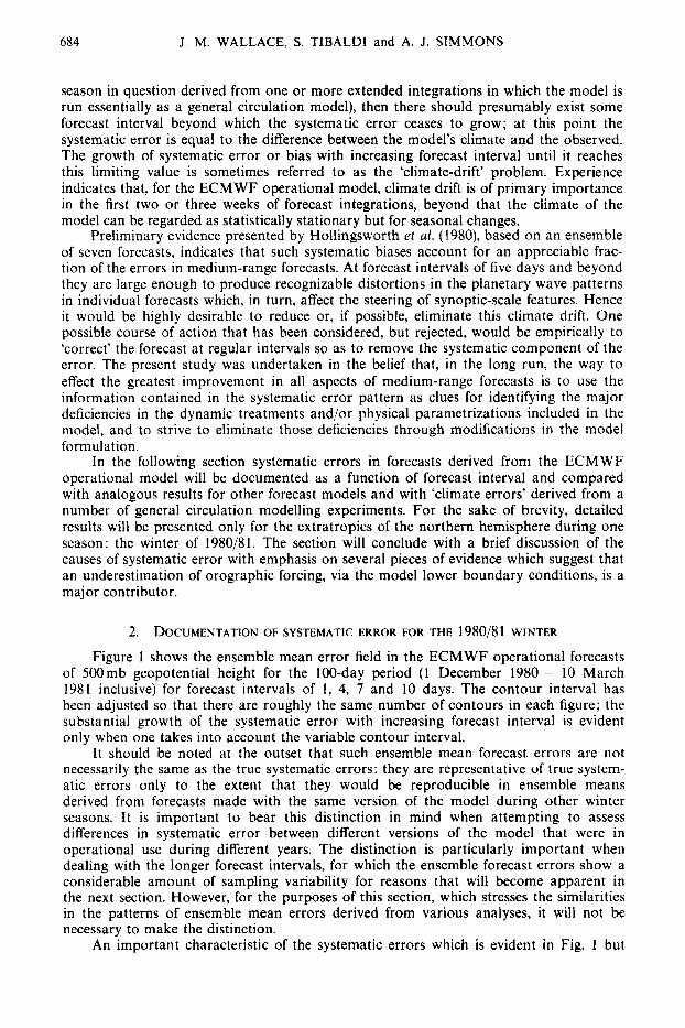
Figure 1 shows the ensemble mean error field in the ECMWF operational forecasts of 500mb geopotential height for the 100-day period (1 December 1980 - 10 March 1981 inclusive) for forecast intervals of 1, 4, 7 and 10 days. The contour interval has been adjusted so that there are roughly the same number of contours in each figure; the substantial growth of the systematic error with increasing forecast interval is evident only when one takes into account the variable contour interval.

It should be noted at the outset that such ensemble mean forecast errors are not necessarily the same as the true systematic errors: they are representative of true systematic errors only to the extent that they would be reproducible in ensemble means derived from forecasts made with the same version of the model during other winter seasons. It is important to bear this distinction in mind when attempting to assess differences in systematic error between different versions of the model that were in operational use during different years. The distinction is particularly important when dealing with the longer forecast intervals, for which the ensemble forecast errors show a considerable amount of sampling variability for reasons that will become apparent in the next section. However, for the purposes of this section, which stresses the similarities in the patterns of ensemble mean errors derived from various analyses, it will not be necessary to make the distinction.

An important characteristic of the systematic errors which is evident in Fig. 1 but

REDUCTION OF ERRORS IN ECMWF MODEL 68 5

Figure 1. Ensemble mean forecast error fields for ECMWF operational forecasts of 500mb height for,the 100-day period (1 December 1980-10 March 1981 inclusive). (a) Day 1 forecasts, contour interval 5m; (b) day 4 forecasts, contour interval 16m; (c) day 7 forecasts, contour interval 30m; (d) day 10 forecasts, contour interval 30m. Background field (lighter contours) is the mean 500mb height field based on ECMWF operational

analyses for the same period, contour interval 80m. Negative contours are dashed.

has not been emphasized in previous studies, is the evolution in the pattern from day 1 to day 10 of the forecast interval. Note, for example, how the centre of negative bias over Europe on day 1 drifts north-westward to north of Scotland on day 4 and subsequently splits into two centres. The rather prominent systematic errors over Asia in the day 1 pattern grow much less rapidly than the errors elsewhere so that by day 4 their signature has virtually disappeared.

The growth of systematic errors during the early part of the forecast interval is approximately linear in the sense that the day 2 errors (not shown) exhibit a pattern similar to the day 1 errors (Fig. l(a)) and are approximately twice as large. In the latter part of the forecast interval (Figs. l(c) and (d)), the systematic errors show a strong negative spatial correlation with the (time-averaged) stationary wave* pattern, as can be

* In this paper the term ‘stationary waves’ denotes departures from zonal symmetry in the time-averaged flow for a particular winter unless otherwise stated.

686 J. M . WALLACE. S. TIBALDI and A. J. SIMMONS

infcrrcd from a comparison with the superimposed 500mb height field. To the extent that the time mean flow pattern for this particular winter resembles the long-term climatological mean flow pattern, it would appear the model lacks sufficient forcing to maintain the stationary waves at the proper amplitude. Hollingsworth et al. (1980) and Derome (1981) have also noted this particular characteristic of the systematic error pattern.

There is also a zonally symmetric component in the error pattern, particularly for the longer forecast intervals, with prevailing negative biases around 50-60"N. A t latitudes near 40"N the zonally averaged gradient of geopotential height is too strong in the forecasts, from which i t may be inferred that the westerlies are too strong at these latitudes.

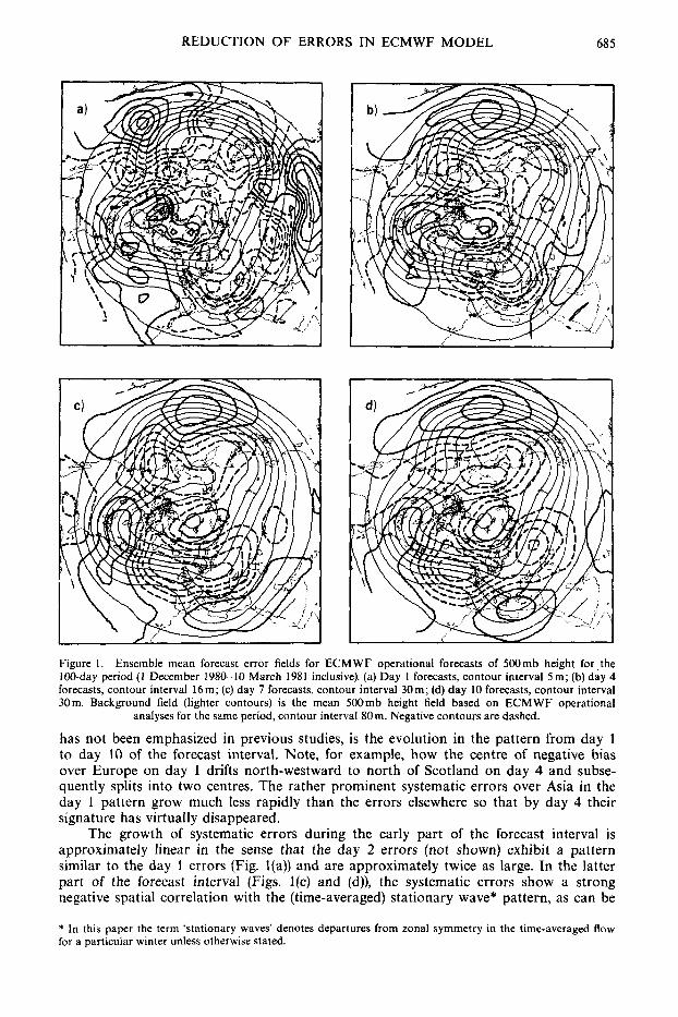
One can obtain some further insight into the systematic errors by comparing the mcan of the day 10 500mb forecasts for the same 100-day period with the mean of the corresponding verification charts, both of which are shown in Fig. 2. It can be seen that the model does succeed in simulating the major features of the time mean pattern, but i t weakens the ridge extending from the Rockies across the Arctic into Siberia, thus making the flow too zonally symmetric at high latitudes. I t also fails to simulate the ridge over the eastern Atlantic and thc split flow further to the east.

F'igure 2. Ensemble mean 500mb height lields for the Fig. 1 IOO-day period. (a) ECMWF operational analyses; (b) day 10 forecasts. Contour interval ROm.

Figurc 3 shows thc pattern of systematic error in the day 1 and day 10 forecasts for the 1000 and 300mb levels, from which i t can be seen that the error field has a qualitat- ivcly similar structurc at the two levels and that the amplitude incrcascs with height. The same 'equivalent barotropic' vertical structure is observed throughout the forecast interval. Although the errors at l000mb are smaller than those at upper levels. they arc associated with substantial distortions in the low-level flow pattern, as is evident from a comparison of the mean of observed and day 10 forecast IOOOmb height maps, shown in Fig. 4. In the forecasts thcre is too much westerly flow across western Canada and across Europe and Central Asia. The Icelandic low is too strong and too far south and the ridge of high pressure that separates it from the Aleutian low is not sufficiently well developed.

The results described above for the 7- and 10-day forecast intervals are in general agreement with patterns derived by Hollingsworth er al., from a sequence of seven ten-day forecasts with two models with different physical parametriLation schemes, and by

REDUCTION OF ERRORS IN ECMWF MODEL 687

Figure 3. Ensemble mean day 1 and day 10 forecast error fields for the Fig. 1 100-day period. (a) 1OOOmb height, day 1 error, contour interval 2Om; (b) 300mb height, day 1 error, contour interval 40m. (c) and (d) as (a) and (b), but for day 10, and superimposed on the corresponding analysed mean fields (lighter contours; intervals

30m and 160m respectively). Negative contours are dashed.

Derome, though there are some minor differences which are probably associated with sampling fluctuations. Extended integrations of the ECMWF model with a number of different horizontal and vertical resolutions also yielded similar departures from the observed climate (Cubasch 1981).

Similar results for the GFDL model were reported by Manabe and Terpstra (1974) and Blackmon and Lau (1980). Pitcher et al. (1983) have shown that means derived from perpetual January runs with the NCAR ‘Community Climate Model’ show similar biases relative to the observed climate.

The day 4 systematic error pattern (Fig. l(b)) can be compared with day 3 errors derived from a number of different operational forecast models and compiled and presented by Bengtsson and Lange (1982). For the most part, the results for the various models are rather similar, with pronounced negative biases over the west coasts of Canada and


Figure 4. Ensemble mean l00Ornb height fields for the Fig. 1 100-day period. (a) ECMWF operational analyses; (b) day 10 forecasts. Contour interval 2 0 ~ .

Europe, in agreement with results presented above*. There appears to be nothing available in the literature for comparison with the day 1 systelhatic error pattern (Fig. l(a)) but T. Bettge (personal communication) has reported to us that the spectral model currently in use at the U.S. National Meteorological Center has a day 1 systematic error pattern during the 1980/81 winter season remarkably similar to that shown in Fig. l(a).

The similarity of the systematic error patterns in the various operational numerical weather prediction models and general circulation models may be a reflection of certain deficiencies in dynamical treatments and/or physical parametrizations which are common to all the models. Certain characteristics of the error pattern are suggestive of deficiencies in the treatment of mountains, namely: (1) At the longer forecast intervals the pattern is suggestive of inadequate forcing for the maintenance of the stationary waves, in agreement with results previously obtained by Hollingsworth et al. (1980) and Derome (1981) with the ECMWF global model. It has been established on the basis of GCM experiments (Kasahara and Washington 1969; Manabe and Terpstra 1974; Held 1983) and studies with simpler models (Charney and Eliassen 1949; Bolin 1950; Grose and Hoskins 1979; Held 1983) that mountains are one of the three major sources of forcing for the extratropical stationary waves, the others being thermal contrasts between land and sea, and Rossby-wave propagation from lower latitudes. ( 2 ) GCM simulations by Manabe and Terpstra (1974) and by Held (1983) indicate that the orographic contribution to the stationary wave pattern is mainly in zonal wavenumbers 2 and 3 and is nearly equivalent barotropic in its vertical structure, whereas the thermal contribution is chiefly in zonal wavenumber 1 and shows a strong westward tilt with height. Hence the horizontal scale and vertical structure of the systematic error pattern is more consistent with a relation to the orographic forcing. The possibility that tropical forcing might play a role cannot, on the contrary, be ruled out on the basis of these arguments, since the remote response to such forcing also displays an equivalent barotropic vertical structure (Hoskins and Karoly 198 1). (3) The day 1 systematic error pattern (Fig. l(a)) shows pronounced negative biases over

* Some of the models have more complicated systematic error signatures. For example, the NMC model in use during the 1970s failed to maintain the thermal contrast between high and low latitudes and between continents and oceans. Because of this strong thermal component, the loo0 and 500mb systematic error patterns were rather different (Wallace and Woessner 1981). Yet despite these additional complications many of the features in Fig. l(b) also appear in the corresponding distribution for the NMC model.


the Rockies and near the Alps, Caucasus and Tien-Shan ranges. Since the compression of air columns in regions of upslope flow and the stretching of air columns in regions of downslope flow should generally result in the generation of anticyclonic vorticity over regions of high terrain, the algebraic sign of the day 1 errors in the vicinity of these mountain ranges is suggestive of an underrepresentation of the height of the smoothed topography used in the model formulation. The statistics presented in the first column of Table 1 give some indication of the height of these ranges as represented in the model during the 1980/81 winter. Note that it is rugged ranges such as the Alps and Canadian Rockies that are grossly underrepresented; high plateaus such as Greenland are less affected by the smoothing. Likewise, it is these rugged ranges which exhibit the large negative systematic forecast errors at day 1.

Lest the negative biases over the mountain ranges in the day 1 error pattern be stressed too strongly, it should be noted that there are large positive biases near and downstream of the Himalayas and at least two of the major features in the day 1 error pattern (the positive biases over the eastern Pacific and the negative biases over northern Japan) occur over regions distant from major mountain regions. Whether these features should be regarded as part of a wave pattern set up by the inadequate treatment of the mountains or as a manifestation of some other source of error in the model is not yet clear.

TABLE 1. APPROXIMATE MAXIMUM TERRAIN HEIGHT (IN METRES) IN SELECTED

REFERS TO THE VERY SMOOTH OROGRAPHY IN USE IN THE ECMWF OPERATIONAL MODEL REGIONS I N THREE DIFFERENT PRESCRIPTIONS OF THE EARTH’S OROGRAPHY. ‘OLD’

PRIOR TO APRIL 1981, ‘OPERATIONAL’ REFERS TO THE OROGRAPHY USED OPER- ATIONALLY FROM APRIL 1981, AND THE ‘ENVELOPE’ OROGRAPHY IS DESCRIBED IN

SECTION 6.

Old Operational Envelope

Alps 500 1400 2700 Greenland 2400 3000 3 200 Rockies (Alaska) loo0 I300 2700 Rockies (Colorado) 2200 2500 3500 H i m a l a y a s 5200 5300 7000

In the following section further empirical evidence will be presented linking the day 1 error pattern to the model’s treatment of rough mountain ranges.

3. ROLE OF MOUNTAINS IN THE DAY 1 ERRORS

If the excessive smoothing of the more rugged mountain ranges is indeed a major contributor to the distinctive signature in the day 1 systematic error pattern, then it seems reasonable to expect that the negative errors over such ranges should tend to be large on days when the flow is particularly strong. In order to test this hypothesis, the 500mb height analyses for the 1980/81 winter were composited in accordance with the general character of the flow patterns in the vicinity of the Rockies and Alps. The compositing procedure, which was entirely subjective, was carried out without any reference what- soever to the forecast or forecast error maps.

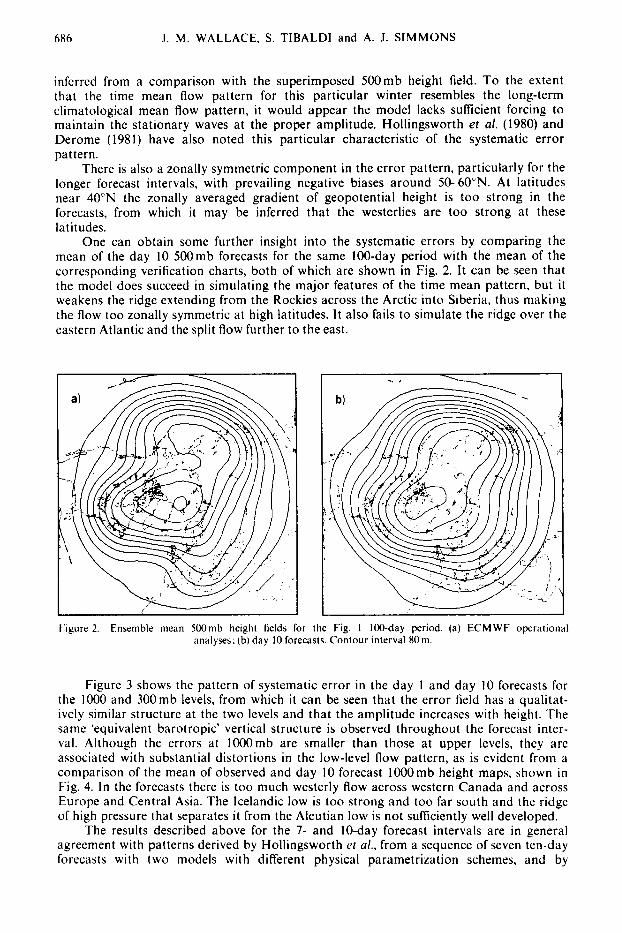
Figure 5 shows the day 1 forecast errors for four different composites based on the observed 500mb flow pattern over the Rockies on the days that the forecasts verified. The dates included in the composites are listed in the figure caption and the four composite 500 mb height patterns are superimposed on the respective forecast error maps. We chose to display and discuss the systematic error mostly at 500mb because this is still the level most commonly used by operational forecasters, and the level where model comparison studies have been mostly carried out. The first composite (Fig. 5(a)) is characterized by a strong zonal flow crossing the Rockies over the north-western United States; the second by a weak ridge over western North America with the jet stream crossing the Rockies


Figure 5. Composite day 1 forecast errors in 500mb height (heavier contours) superimposed upon the corresponding composite 500mh analyses a t verification time. (a) 1-3 December 1980, 14-18 February 1981; (h) 1 I , 13, 14, 15,26,28,30 December 1980, 20 January, 13.21, 22 February 1981; (c) 31 December 1980, 1,2, 7-19, 21, 25, 26, 30, 31 January, I , 2, 25 February, 2, 9, 10 March 1981; (d) 1-6 December 1980, 29, 30 January, 5-10, 24, 25 February 1981. Contour intervals 10m for errors, 80m for 500mb height fields. Negative contours are

dashed.

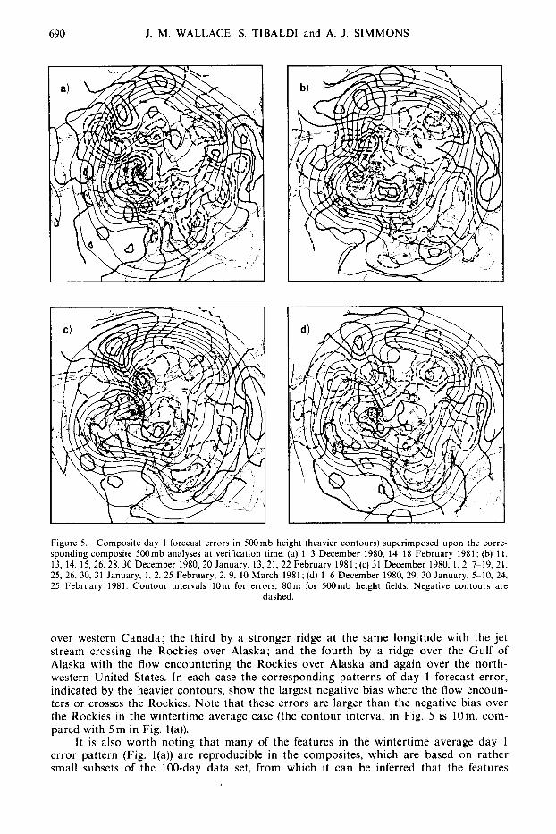
over western Canada; the third by a stronger ridge at the same longitude with the jet stream crossing the Rockies over Alaska; and the fourth by a ridge over the Gulf of Alaska with the flow encountering the Rockies over Alaska and again over the north- western United States. In each case the corresponding patterns of day 1 forecast error, indicated by the heavier contours, show the largest negative bias where the flow encoun- ters or crosses the Rockies. Note that these errors are larger than the negative bias over the Rockies in the wintertime average case (the contour interval in Fig. 5 is 10m, compared with 5 m in Fig. l(a)).

It is also worth noting that many of the features in the wintertime average day 1 error pattern (Fig. l(a)) are reproducible in the composites, which are based on rather small subsets of the 100-day data set, from which it can be inferred that the features


apparent in Fig. l(a) are of high statistical significance, despite their complexity and their relatively small absolute magnitude. Hence it appears that much smaller data samples than the 100 forecasts used as a basis for Fig. l(a) may be sufficient for assessing the gross features of the systematic error patterns in short-term forecasts.

Composites similar to those shown in Fig. 5 were prepared for various flow regimes over the Alps and it was found that the negative biases in the day 1 forecasts tend to be largest (up to about 60m) under conditions of strong north-westerly flow. Presumably, a similar situation exists for the Himalayas, but we did not produce composites for that region.

Composite forecast error maps can also be generated for longer forecast intervals, but the definition of what constitutes the effective mean flow becomes increasingly ambig- uous as the forecast interval lengthens. This ambiguity ultimately undermines the very basis for defining the composites.

4. SYSTEMATIC ERRORS DURING THE 1981/82 WINTER

A major change in the representation of orography was introduced into the ECMWF operational model in April 1981. Prior to that time a highly smoothed orography, originally designed for models with a rather coarse spatial resolution, had been in use. The revised orography was designed to be compatible with the spatial resolution of the ECMWF model (1.875" of latitude and longitude in the operational (N48) version). It was constructed from a recently released U.S. Navy global high-resolution (2 latitude x 2 longitude) data set by simple area averaging. The N48 mean orography was then smoothed with a Gaussian-shaped grid point filter in order to eliminate small-scale features that the model would interpret as noise. (A detailed documentation is given in Tibaldi and Geleyn (1 98 1))

The second column of Table 1 gives a rough indication of the height ot some or tne major mountain ranges in the revised prescription of the orography. It is evident that this rougher 'revised orography' is still rather low in comparison to what might be regarded as the effective height of ranges such as the Rockies and Alps, but the increase relative to the 'old orography' is substantial in some cases.

Error patterns analogous to those described in the previous sections were computed for the 1981/82 winter. Results (not shown) indicate that at day 1 the error pattern was very similar to that for the previous winter. At day 10 the patterns for the two winters showed some pronounced differences, but it is not clear whether these were due to the change in the prescription of the mountains, or to the substantial differences between the hemispheric circulation patterns which prevailed during the two winters.

5. EXPERIMENTS WITH A BAROTROPIC MODEL

It was shown in Fig. 1 that the spatial signature of the systematic forecast error undergoes substantial evolution as it amplifies through the first ten days of the forecast interval. Whereas at day 1 i t shows a rather consistent relation to the major mountain ranges, by day 10 it seems to be more closely related to the observed stationary wave pattern and the relation to the mountains is less direct and less obvious. The hypothesis that there is excessive smoothing of the earth's orography in the model formulation would be put on firmer ground, so to speak, if the evolution of the systematic error through the forecast interval could be interpreted as a response to a steady forcing whose spatial signature bore a direct relation to the forcing, as represented by the mountains. Experi- ments with a barotropic model to be described in this section, provide support for such an interpretation.

These barotropic experiments are of a type similar to those reported by Simmons (1982) in a study of the mid-latitude response to tropical forcing. Typically, a basic state varying with both latitude and longitude is chosen, and a forcing of the barotropic model

692 J. M. WALLACE, S. TIBALDI and A. J . SIMMONS

is determined such that this state remains stationary when used as initial conditions for the model. The response of this forced state to the initiation of an additional steady forcing is then examined. Model details are as described by Simmons, apart from the use of a larger linear dissipation rate, (5 d)- I. The choice of the 300 mb level for applying the barotropic model was made for reasons discussed in Simmons et al. (1983).

The principal experiment discussed here has as the forced basic state the 300mb streamfunction averaged over the 100-day period from the winter of 1980/81 referred to in section 2 (see Fig. 3(b)). The additional forcing is at a rate identical (apart from a modification discussed in appendix A) to the mean rate of error growth in the 300mb streamfunction over the first day of the operational forecasts verifying in the 100-day period. The experiment thus suggests the extent to which the systematic error for the latter part of the forecast period may be regarded as the response to the erroneous forcing that is indicated by the initial growth of mean error.

The response after 4 and 10 days of forcing is shown superimposed on the basic state in Fig. 6 . Comparison with Figs. 1 and 3 shows that this response does indeed bear a clear similarity to the evolution of systematic error through the forecast period. Common features worthy of note are the regions of positive error (or response) over the central Pacific and the eastern part of North America, the major negative region centred west of Europe, and the negative region extending over the North Pacific and western North America, although by day 10 the centres of these regions are located further west in the forecast errors than in the barotropic calculation. The simpler model successfully captures the absence of any significant growth of the initial negative error near the Asian coast, but fails to simulate the development of a third low centre north of the Caspian Sea towards the end of the 10-day period.

Caution must be exercised when comparing the magnitude of the barotropic response with the growth of the systematic forecast error. The latter shows a general negative bias due to an overall model cooling which cannot be reproduced by the barotropic model (see again appendix A), and also a somewhat smaller amplitude of the error

DRY Lf DRY 10

Figure 6. Perturbation height fields (heavy solid, dashed) for the northern hemisphere at day 4 (contour interval 20m) and day 10 (countour interval 40m). Heights are defined from the linear balance equation as discussed in appendix A, and negative contours are dashed. The thin solid lines represent the streamfunction of

the basic state, and the contour interval corresponds to a geostrophic height interval of 120m at 45"N.


pattern. The amplitude of the barotropic response is sensitive, however, to the level at which the model is applied and to the amount of dissipation used. The response is increased by use of weaker dissipation and decreased by use of a level lower than 300mb, although arguments advanced by Held (1983) favour use of a level higher than the traditional 500mb. It is difficult to know quite what are the best choices for model parameters, and this uncertainty should be kept in mind. In addition, the relevance of the part of the response forced from the tropics is rather unclear.

Figure 7 shows the response after 10 days to that part of the forcing located poleward of 20"N (left) and that part located in the band between 20"N and 20"s (right). Since forcing from the extratropics of the southern hemisphere (not shown) has a negligible effect on the extratropical northern hemisphere, and since the overall barotropic response is largely linear, this figure thus shows the portion of the day 10 pattern shown in Fig. 6 which is forced from middle and high latitudes of the northern hemisphere, and the portion forced from the tropics.

n w i n DRY 10

Figure 7. The day 10 response to forcing located north of 20"N (left) and between 20"N and 20"s (right). Other details as for Fig. 6.

A striking feature of Fig. 7 is the similarity between the wave patterns forced from the two regions. This may be understood partially in terms of idealized barotropic forcing experiments described by Simmons (1982), and further experiments (Simmons et al. 1983), which indicate that in the presence of a basic state with longitudinal variations there are preferred regions and patterns of response. Such calculations do not, however, indicate why the two patterns shown in Fig. 7 should be of the same sign. Rather, it appears that the tropical forcing, which has negative maxima over the western Pacific and northern South America, excites wave trains over and downstream of the Pacific and Atlantic Oceans, and these wave trains reinforce, perhaps coincidently, the extratropically forced wave pattern.

In interpreting the response to the tropical component of the forcing, it is necessary to keep in mind the nature of the forcing, which is computed as the mean difference between the day 1 forecasts and initialized verifying analyses. For the extratropics, evidence has been presented indicating that this difference largely represents a systematic bias in the day 1 forecasts due to inadequate orographic forcing in the forecast model. For the tropics, however, some part of the mean difference (or error) may be due not to an inherently erroneous model forcing, but to an unrealistic initial distribution of convective


heating arising from the operational use of an adiabatic initialization procedure during the period in question. If so, it would be inappropriate to force the barotropic model steadily over a 10-day period with the one-day forecast error and the relatively large extratropical response to the tropical component of the forcing does not necessarily indicate the extent to which a deficiency in the modelling of tropical convection influences the extratropical systematic error.

Notwithstanding the above considerations, the similarity of the two forced patterns shown in Fig. 7 has important consequences for the strategy to be adopted when seeking to improve a model. If two sources of error may contribute in a similar way to an overall error pattern, the danger of tuning one source, say the orography, to reduce systematic errors in the later part of the forecast interval is evident. A better course of action in the case of the orography, for example, would be to seek to minimize the short-range forecast error in the vicinity of rugged terrain.

D A Y Lf DRY Li

D A Y 10 D A Y 10

Figure 8. The response at day 4 (contour interval 20m) and day 10 (contour interval 30m) due to forcing from the ‘American sector’, as defined in the text, (left) and the ‘Eurasian sector’ (right).


Although the response shown in Fig. 6 differs little from day 4 to day 10 the dominant source of the response observed at a particular geographical location varies substantially over this later part of the forecast interval. Figure 8 shows the response at days 4 and 10 due to forcing poleward of 20 ON in the longitude ranges 180 OW-60 OW (the ‘American’ sector, shown left) and 60 OW-180 “E (the ‘Eurasian’ sector, right). These, and related calculations, show that at day 4 the predominant forcing of the negative forecast errors over northern Europe and North America is the local forcing in their respective sectors, which has been linked with the treatment of the orography in these regions. By day 10, however, a hemispheric pattern is set up in response to the forcing from both sectors, with a somewhat larger amplitude excited from the American sector. The overall similarity of the two day 10 patterns should again be noted.

A number of calcuiations have been performed to assess the sensitivity of the response of the barotropic model to changes in the background flow and its associated forcing, and to changes in the additional steady forcing that is imposed. Resulting day 10 error fields for two such experiments are shown in Figs. 9 and 10. Figure 9 is based on a repeat of the primary calculation shown in Fig. 6, but for the winter of 1981/82. Some differences in detail are found between the results for the two winters, with a weaker amplitude and westward phase shift of the pattern for the later winter. Whilst these differences are in the same sense as those in the systematic errors for the t w o winters, the two barotropic calculations are generally more similar to one another than are the two corresponding forecast error maps.

DRY 10 DRY 10

Figure 9. The response at day 10 (contour interval 40m) from calculations for the 1981/82 winter (as

Fig. 6 , right, but for 1981/82 instead of 1980/81).

Figure 10. As in Fig. 9, but with the zonally- varying component of the basic mean state sup-

pressed. See also text, section 5.

Figure 10 is based on a repeat of the 1981/82 calculation, but with the longitudinally- varying (or stationary-wave) component of the basic mean state suppressed. The much weaker amplitude and the zonal orientation of the resulting wave pattern highlights the crucial role played by the longitudinal variation of the basic state, and is in agreement with the experiments described by Simmons (1982) and Simmons et al. (1983). Interme- diate calculations, in which the 1980/81 and 1981/82 forcings were superimposed on a climatological, but longitudinally-varying, basic state, gave results largely similar to those


shown for the actual mean winter states (Figs. 6 and 9) although agreement with the corresponding systematic errors was somewhat poorer. Finally, a series of experiments has been performed in which actual mean states were used, but with the phase of the forcing shifted by various amounts. Some of the characteristic wave trains identified in the idealized experiments could again be seen, but the signs of the responses, and the relative amplitudes of the Pacific and Atlantic patterns, were such that the overall forced patterns generally bore little resemblance to the pattern of systematic forecast errors. These supple- mentary experiments thus show that the response resembling the systematic errors is not an inevitable feature of the barotropic model, and they indirectly support the hypothesis that a steady forcing determined by the rate of growth of the systematic error during the first day of the forecast interval can account for the gross features of the time evolution of the systematic error pattern through the remainder of the forecast interval.

6. CONCEPT OF AN ENVELOPE OROGRAPHY

The empirical evidence presented in the previous sections reinforces the impression that even the newer prescription of the earth’s orography in the ECMWF grid-point model does not adequately represent the dynamical influence of the earth’s major mountain ranges upon the large-scale motions. Specifically, what appears to be lacking is the effect of high terrain features on the sub-grid scale in blocking the large-scale flow and thereby providing a favourable environment for weaker, mesoscale circulations in the neighbouring basins and valleys. It seems plausible that these sheltered regions, which are often capped by inversions and stratus cloud layers during wintertime, should be effec- tively decoupled from the large-scale flow over the mountain range. It has been suggested by Mesinger (1977), Bleck (1977) and others that such unresolved mesoscale circulations might be parametrized in large-scale numerical weather prediction models by treating the sheltered basins and mountain valleys as though they were part of the terrain itself: hence the notion of an ‘envelope orography’.

The vertical extent of such orographically forced mesoscale circulations changes from day to day in response to shifts in direction of the large-scale flow relative to the orientation of the significant terrain features and to changes in static stability. Hence the optimal formulation of an envelope orography is by no means obvious. As a basis for a series of numerical experiments to be described in the following two sections, a decision was made to adopt a very simple formulation, which does not take such day to day variability into account. We are indebted to our colleague, J.-F. Geleyn, for, among other things, pointing out than an envelope orography which has a number of desirable features can be created simply by adding, before the final smoothing operation, to the conventional N48 area mean orography an additional increment equal to a constant times the sub-grid-scale standard deviation of the high resolution orography about its N48 grid-point mean value. ( I t subsequently came to our attention that Mesinger and Strickler (1982) employed a similar formulation in experimental forecasts of cyclogenesis in the lee of the Alps and obtained encouraging results.) For an idealized sub-grid-scale orography consisting of a pure two-dimensionally sinusoidal mountain range*, it is readily verified that a constant of 2.0 would yield a true envelope orography whose height is equal to that of the mountain tops. Such a formulation is appealing in the sense that the envelope increment is largest for rough mountain ranges, which appear to be the most seriously underrepresented in the conventional smoothed orography, whereas it is smaller for high plateaus such as Greenland and Antarctica, which appear to be adequately represented in the area-mean formulation. It also has the desirable property of being resolution depen- dent: as the horizontal resolution of a model is increased, so that it explicitly resolves

* Terrain height proportional to coskxcosly where x and y are orthogonal horizontal coordinates and k and I are horizontal wavenumbers in the directions of those coordinates (k + 0, I i: 0).


smaller-scale terrain features, the envelope increment automatically decreases, as physical reasoning suggests that it should.

The high resolution orography used as a basis for calculating the envelope increment is the same US. Navy data set mentioned previously. Terrain features not resolved by this 4" grid were taken into account by adding to the variance of the US. Navy data set, calculated with respect to the N48 grid, the term

C pib(hi(max) - hi)(hi - hi(min)}

where h,(max) and hi(min) refer to the maximum and minimum terrain heights within the ith high resolution grid square (these values were also contained in the U.S. Navy dataset), hi is the mean terrain height within that square, the summation is taken over all the high resolution grid points in the N48 grid square and pi is the relative area weight of the ith high resolution grid square.

In the case of an idealized orography of a single scale too small to be resolved at all

0" 20"E

80"E 100"

160" W

140"

120"

100"W

80" N

60"

40"

20"

Figure 11. Envelope orography for three selected regions (contours) superimposed on the high resolution US. Navy orography data set (shading). Upper left: Mediterranean region; contour interval 300111; 1500m contour thickened and used as threshold for shading of high resolution orography. Lower left: Himalayan region; contour interval 500m; 4000m contour thickened and used as threshold for shading. Right: Rockies; contour

interval 300m; 1800m contour thickened and used as threshold for shading.

698 J. M. WALLACE, S. TIBALDI and A. J . SIMMONS

by the U S . Navy grid, this algorithm would yield an 'envelope' N48 height increment of

[{h(max) - h } { h - h(min)}]''2

where the disappearance of the index i indicates that all high resolution grid points within the N48 grid square are taken as having the same values.

The envelope orography so obtained was subjected to the same smoothing procedure as was used for the production of the operational orography (Tibaldi and Geleyn 1981). Maximum heights of selected mountain ranges, as represented in this envelope orography, are shown in the third column of Table 1 . The incremental increase associated with the envelope terms can be inferred by noting the difference between the second and third columns. The largest percentage increases occur over the Alps and northern Rockies where the terrain heights are roughly doubled. Large increases also occur over the Hima- layas and Colorado Rockies, but in these regions the terrain heights are already substantial in the conventional orography. As expected, there is only a small incremental increase in the height of the Greenland icecap.

Figures 1 I and 12 contrast the representation of the operational orography in use in the ECMWF model since April 1981 with the envelope orography for a number of

0" 20"E

40" N

80"E 100" 100"W

Figure 12. As in Fig. 1 1 but for orography introduced into the ECMWF operational model in April 1981 ('operational' orography).


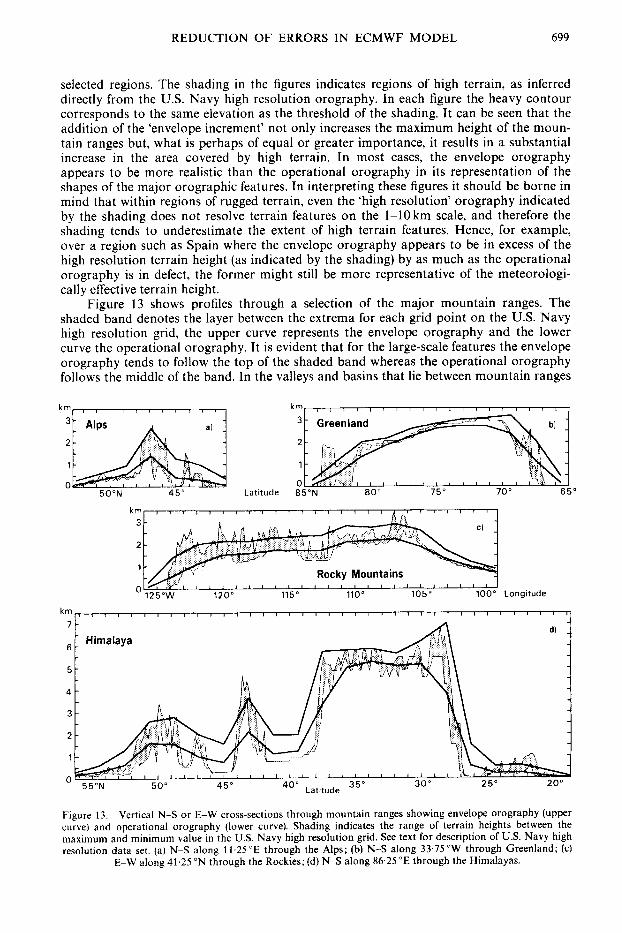
selected regions. The shading in the figures indicates regions of high terrain, as inferred directly from the U.S. Navy high resolution orography. In each figure the heavy contour corresponds to the same elevation as the threshold of the shading. It can be seen that the addition of the 'envelope increment' not only increases the maximum height of the mountain ranges but, what is perhaps of equal or greater importance, it results in a substantial increase in the area covered by high terrain. In most cases, the envelope orography appears to be more realistic than the operational orography in its representation of the shapes of the major orographic features. In interpreting these figures it should be borne in mind that within regions of rugged terrain, even the 'high resolution' orography indicated by the shading does not resolve terrain features on the 1-10 km scale, and therefore the shading tends to underestimate the extent of high terrain features. Hence, for example, over a region such as Spain where the envelope orography appears to be in excess of the high resolution terrain height (as indicated by the shading) by as much as the operational orography is in defect, the former might still be more representative of the meteorologi- cally effective terrain height.

Figure 13 shows profiles through a selection of the major mountain ranges. The shaded band denotes the layer between the extrema for each grid point on the U.S. Navy high resolution grid, the upper curve represents the envelope orography and the lower curve the operational orography. It is evident that for the large-scale features the envelope orography tends to follow the top of the shaded band whereas the operational orography follows the middle of the band. In the valleys and basins that lie between mountain ranges

km

3

2

1

0 50"N 45" Latitude 85"N 80" 75" 70 65"

- Himalaya 6 -

5 -

4 -

Figure 13. Vertical N-S or E-W cross-sections through mountain ranges showing envelope orography (upper curve) and operational orography (lower curve). Shading indicates the range of terrain heights between the maximum and minimum value in the US. Navy high resolution grid. See text for description of US. Navy high resolution data set. (a) N-S along 11.25 "E through the Alps; (b) N-S along 33.75 "W through Greenland; (c)

E-W along 41.25"N through the Rockies; (d) N-S along 86.25 "E through the Himalayas.

700 J. M. WALLACE, S. TIBALDI and A. J. S IMMONS

500' I

't 1 0 1 2 5 10 20 50 100

Wavenumber

Figure 14. Two-dimensional wavenumber spectra of the height of the envelope orography (ENV), and the old and the revised operational orographies (OLD and OPE, respectively). The wavenumber zero values corre-

spond to the mean surface elevations and are indicated by dots.

the envelope lies well above the land surface. Figure 14 contrasts the two-dimensional spectra of the envelope orography (ENV) with that of the old and revised operational orographies (OLD and OPE, respectively). In comparison with the revised operational orography, the envelope orography has higher variance in all wavenum bers. The greatest difference is in the low wavenumbers, particularly wavenumber 1, where the variance is nearly twice as large. It is interesting to note that the revised operational orography has less variance in wavenumbers 2 to 8 than the old orography. The greater prominence of the mountain ranges in the revised operational orography is largely a reflection of the larger variance in the high harmonics. At the higher wavenumbers, the variance in both the revised operational and envelope orographies decreases roughly in proportion to the inverse square of the wavenumber, whereas the variance in the old orography drops off much more steeply ( - K 3 ) .

Numerical experiments based on the envelope orography are described in the following two sections.

7. COMPARISON OF EXTENDED INTEGRATIONS WITH OPERATIONAL AND ENVELOPE

The idea that some sort of enhancement of the earth's orography relative to the conventional, operational orography might result in an improved simulation of the northern hemisphere wintertime climate has been under discussion for some time in various modelling groups. During the late 1970s the Meteorological Office conducted a series of experiments using a 5-level GCM in which the orography was doubled up to a prescribed ceiling increment (1 km north of 63"N and 1.5 km elsewhere). Although the simulation of

OROGRAPHIES


the stationary waves appeared to be substantially improved by the enhancement of the orography, the experiments were not regarded as successful because the hemispheric mean transient eddy kinetic energy, which was already much smaller than the observed in the standard version of the model, was found to be reduced still further by the enhancement of the orography (Hills 1979).

The experiment described below was an effort to make a preliminary assessment of the effect of using an envelope orography in the ECMWF operational model. A single pair of 50-day integrations was carried out, both starting from the same initial conditions (the initialized analysis using FGGE data for 21 January 1979): one experiment employ- ing the conventional, operational orography introduced in April 1981 and the other the envelope orography described in the previous section.

In the latter experiment the envelope orography was inserted into the initial conditions by means of a vertical interpolation of the mass, wind and moisture fields to the a-coordinate system defined by the new envelope lower boundary, temporarily elimi- nating, therefore, most of the PBL over rugged mountains. No attempt was made to allow the system to readjust to the presence of the envelope orography by inserting this orography a few days earlier and running a few data assimilations. Given the GCM nature of this experiment and also given the fact that the first 20 days of the integration were not used to assess the results, such a period of adjustment was not considered necessary. It should also be pointed out that, during the 50 days, the seasonal cycle was frozen at the January value. Only a very limited selection of the results will be presented here. As mentioned above, the analysis of all results was based upon means for the last 30 days of the integrations.

The left-hand panels of Fig. 15 show the mean simulated 500mb height fields for days 21-50 of the two experiments (OPE and ENV) together with the observed 500mb height field for the corresponding period (1 1 Feb.-12 March, OBS). The envelope orography experiment produced a more realistic simulation of the ridge over the Bering Strait, the trough over the Gulf of Alaska and the height pattern over the eastern Atlantic. In certain other respects the two simulated fields more closely resemble one another than they resemble the observed field : neither experiment correctly simulated the split flow in the 0-60"E sector and both generated the same spurious low-latitude short-wave pattern in the 120-18o"W sector. The corresponding 1OOOmb height fields are shown in the right-hand panels of Fig. 15. The most striking differences between the two experiments involve the pattern over North America. The envelope orography simulation shows a pronounced ridge of high sea level pressure just to the east of the Rockies, in agreement with the observed, whilst the operational orography simulation shows an unrealistic pattern characteristic of many GCM simulations, with lo00 mb westerly geostrophic flow extending across the North American continent. This difference may be of significance for understanding one of the most pervasive biases in the intermediate-range forecasts: the failure of the Rockies to act as a barrier to the low-level zonal flow. The envelope orography simulation is also somewhat better over the Atlantic and European sectors. The westerlies do not penetrate into southern Europe as they do in the experiment with the operational orography. Simulated 850 mb temperatures (not shown) were lower over much of the Arctic, in better agreement with the observed. The improvement was particularly pronounced over western and central Canada, in the region shielded from the low-level westerly flow by the envelope orography.

The differences in the zonally averaged statistics for the two experiments are less dramatic than those described above, but the introduction of the envelope orography resulted in some unexpected improvements which are perhaps worthy of note. The zonally averaged jet stream was too strong and too far north in both experiments, but the biases were substantially smaller in the envelope orography experiment. The relevant mean values are summarized in the first two rows of Table 2. The envelope orography experiment also correctly simulated the observed low-level easterlies in the polar cap region, in contrast to the control experiment. The zonally averaged temperature distribu-

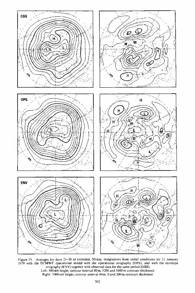
Figure 15. Averages for days 21-50 of extended, SO-day, integrations from initial conditions for 21 January 1979 with the ECMWF operational model with the operational orography (OPE), and with the envelope

orography (ENV) together with observed data for the same period (OBS). Left: 500mb height, contour interval 80m, 5200 and 5600m contours thickened. Right: lOOOmb height, contour interval 40m, 0 and 200m contours thickened.

70?

REDUCTION OF ERRORS IN ECMWF MODEL

TABLE 2. SELECTED STATISTICS FOR DAYS 21-SO OF EXTENDED RUNS WITH OPERATIONAL MODEL (OPE), ENVELOPE OROGRAPHY (ENV), AND OBSERVATIONS

POSPHERIC JET STREAM; emax THE LATITUDE OF THE TROPOSPHERIC JET STREAM;

HEMISPHERE SO0 mb HEIGHT FIELD.

FOR THE CORRESPONDING PERIOD (OBS). u,,, DENOTES THE SPEED OF THE TRO-

AND R.M.S. THE ROOT MEAN SQUARE TRANSIENT VARIABILITY OF THE NORTHERN

45 50 47 27 35 32 10.06 1 1.46 10.77

703

tion was also more realistic in the envelope orography experiment: the polar lower troposphere was up to 5 K colder and in much better agreement with the observed, and most of the remainder of the troposphere was slightly warmer, but not quite warm enough. If these experiments can be regarded as representative, the overall bias towards a cold troposphere might be reduced by as much as 50% by the introduction of the envelope orography. The extratropical stratosphere was much too cold in both simulations; the bias was up to about 15% larger in the envelope orography experiment.

In view of the prior experience of the Meteorological Office group, a major source of concern in the introduction of an envelope orography or any other enhanced orography was the possibility of an unrealistic drop in the amplitude of the transient eddies. The third row of Table 2 shows the hemispherically integrated transient eddy variability of 500mb height in the two simulations, together with the observed value. Two facts emerge clearly: the relative decrease in 500 mb height transient wave variance brought about by the insertion of the envelope orography is not nearly as worrying as in the aforemen- tioned experiment; the level of transient wave activity in the control run, instead of being already far too low, was in fact slightly too high. As a consequence, insertion of the envelope orography in fact improves the mean level of transient wave activity. The horizontal structure is, moreover, also improved, as shown in Fig. 16 . The main deficiencies of the OPE transient wave pattern, compared with the OBS map, are: the absence of an Atlantic storm track (represented by the observed maximum of 27 dam near 50"W); the band of excessive values over Canada and the north-eastern Pacific; and the weak values over northern Europe. A comparison between OPE and ENV in Fig. 16 shows that all these deficiencies, if not completely cured, have been substantially improved by the envelope orography.

In view of the short length of this experiment, the statistical significance of the results is open to question. Nevertheless, the fact that the simulation with the envelope orography yielded a climate that is in many respects more realistic than that derived from the control experiment was viewed as encouraging. Rather than conducting additional GCM experiments designed to test the reproducibility of these results, a decision was made to test further the usefulness of the envelope orography formulation by means of a series of numerical weather prediction experiments, which we now describe.

8. A NUMERICAL PREDICTION EXPERIMENT WITH THE ENVELOPE OROGRAPHY

The organization of the numerical prediction experiment is shown in Table 3. The envelope orography was inserted into data assimilation cycles, starting with the analysis for 1 2 0 0 ~ ~ ~ on 20 January 1982 and from that time onward ten-day forecasts were generated at daily intervals which could be compared with control runs generated in real time by the operational forecast model with the conventional operational orography introduced in April 1981. Analysis and initialization were carried out at 6-hour intervals throughout the experiment, just as in the operational runs but using, as first guess fields, 6-hour forecasts generated by the model with the envelope orography. The last day for which forecasts with the envelope orography were generated was February 9. For ease of


OPE 1

Figure ments

16. Temporal (transient wave) variance of 500mb geopotential height for the extended range experi- presented in Fig. 15. Averages for days 21-50. OBS: observed; OPE: operational orography; ENV:

envelope orography. Units are decametres throughout; contour interval 8 dam.

TABLE 3. ORGANIZATION OF FORECAST EXPERIMENTS. CROSSES DENOTE DATES ON WHICH FORE-

IDENTIFIED I N FIG. 19; ‘EPOCH’ DENOTES COMPOSITE WHICH FORECASTS FOR THAT DATE ARE GROUPED CASTS WERE MADE; ‘CODE’ DENOTES LETTER BY WHlCH FORECASTS STARTED ON THAT DATE CAN BE

IN FIGS. 20 AND 2 1.

1982 Code Epoch 1982 Code Epoch

20 Jan. x 29 Jan. x I 21 Jan. x A 30 Jan. x J 22 Jan. x B 31 Jan. x K I 23 Jan. x C 1 Feb. x L I 24 Jan. x D 2 Feb. x M I 25 Jan. x E 3 Feb. x N I1 26 Jan. x F 4 Feb. x 0 I1 27 Jan. x G 5 Feb. x P 11 28 Jan. x H 6 Feb. x Q I1

1982 Code Epoch

7 Feb. x R I1 8 Feb. x S I1 9 Feb. x T 111

10 Feb. u 111 11 Feb. v 111 12 Feb. w IV 13 Feb. x IV 14 Feb. Y 1v 15 Feb. z 1v


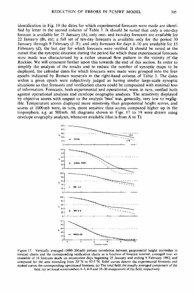
identification in Fig. 19 the dates for which experimental forecasts were made are identified by letter in the second column of Table 3. It should be noted that only a one-day forecast is available for 21 January (A), only one- and two-day forecasts are available for 22 January (B), etc; a full set of ten-day forecasts is available only for the period 30 January through 9 February (J-T); and only forecasts for days 6-10 are available for 15 February (Z) , the last day for which forecasts were verified. It should be noted at the outset that the synoptic situation during the period for which these experimental forecasts were made was characterized by a rather unusual flow pattern in the vicinity of the Rockies. We will comment further upon this towards the end of this section. In order to simplify the analysis of the results and to reduce the number of synoptic maps to be displayed, the calendar dates for which forecasts were made were grouped into the four epochs indicated by Roman numerals in the right-hand column of Table 3. The dates within a given epoch were subjectively judged as having similar large-scale synoptic situations so that forecasts and verification charts could be composited with minimal loss of information. Forecasts, both experimental and operational, were, in turn, verified both against operational analyses and envelope orography analyses. The sensitivity displayed by objective scores with respect to the analysis 'bias' was, generally, very low to negligible. Temperature scores displayed more sensitivity than geopotential height scores, and scores at l000mb were, in turn, more sensitive than scores computed higher up in the troposphere, e.g. at 500mb. All diagrams shown in Figs. 17 to 19 were drawn using envelope orography analyses, whenever available (that is from A to T).

.............................. ENV

- - _ - - _ _ - _ 40

20 OPE - - a1 TOTAL

...........

40

20 bl ZONAL PART

%

- - -. - _ 40 - 2 0 - dl W N 4-9

0' ' 2 b 6 8

_--_. -0

Forecast days

Figure 17. Vertically averaged (1000-200mb) pattern correlation between geopotential height anomalies in forecast charts and the corresponding verification charts as a function of forecast interval, averaged over an ensemble of 16 forecasts made on consecutive days beginning 25 January and ending 9 February 1982, and computed for the area extending from 2O"N to 82.5"N. Solid curves denote the experimental forecasts and dashed curves the corresponding operational forecasts. (a) The total field; (b) zonally averaged component of the

field; (cHe) zonal wavenumbers 1-3,4-9 and 10-20 components of the field, respectively.


In view of previous experience with studies of this type it was judged that a period of at least five days would be required for the forecast fields to adjust fully to the vertical interpolation necessary to insert the envelope orography. Therefore, results involving forecasts made during the first four days of the experiment were not taken into account in the evaluation of the experiment.

Figure 17 shows several measures of forecast skill plotted as a function of forecast interval for an ensemble of 16 pairs of consecutive forecasts beginning with those made on 25 January, five days after the insertion of the envelope orography, and ending with those made on 9 February, the last day on which experimental forecasts were made. The scores are based on anomaly correlations between forecast charts and the corresponding verification charts averaged over the 20-82.5"N latitude belt for the parameter in question. For reference it is perhaps worth noting that forecast fields with ensemble-average anomaly correlations in excess of 60% are usually considered to be operationally useful, at least under most circumstances. Scores for the experimental forecasts with the envelope orography are indicated by solid curves and those for the operational control runs by dashed curves. In all the cases considered here the forecast scores are far better than persistence except for wavenumber band 10 to 20 (Fig. 17(e)) and towards the latter part of the forecast period, after day 8, when some of the forecast scores drop below zero.

The top panel in Fig. 17 shows results for geopotential height at individual levels between 1000 and 200mb, vertically averaged to form a single score. By this measure of skill, the experimental forecasts became distinguishably better by day 49 and remain so until the end of the forecast period. The anomaly correlation for the experimental forecasts remains above 60°% until day 6$, about a half a day longer than it did for the operational forecasts.

The next four panels show the corresponding scores for the zonally averaged component of the geopotential height field and the zonal wavenumber bands 1-3, 4-9 and 10-20 components. The results for the zonally averaged component and for wavenumbers 1-3 and 4-9 show roughly the same amount of improvement as the total field; and the results for wavenumbers 10-20 show, if anything, a slight deterioration of the shorter- range forecasts due to the introduction of the envelope orography.

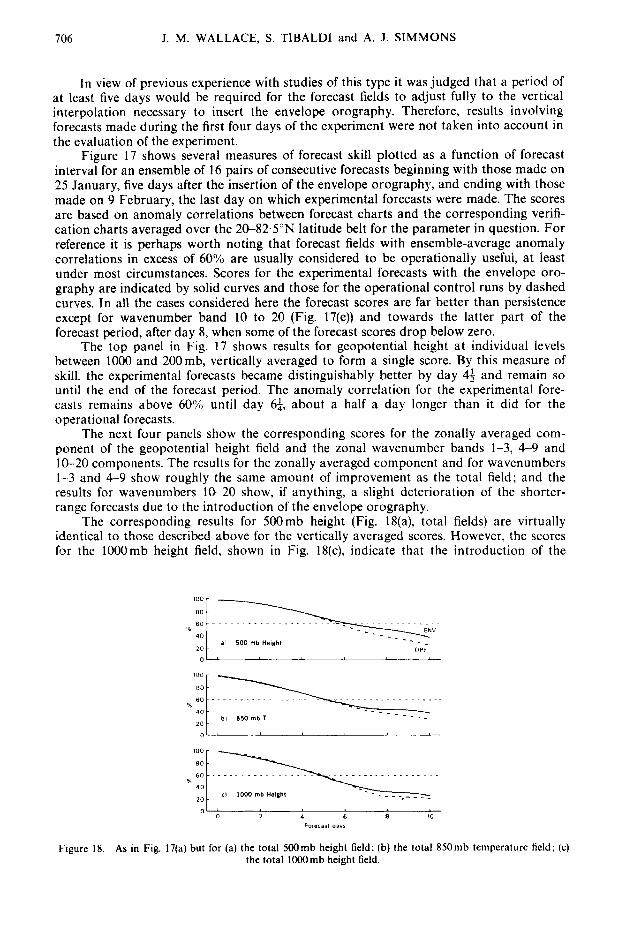
The corresponding results for 500mb height (Fig. 18(a), total fields) are virtually identical to those described above for the vertically averaged scores. However, the scores for the 1OOOmb height field, shown in Fig. 18(c), indicate that the introduction of the

0'

o l ' 0 2 4 6 8 I0

Forecast days

Figure 18. As in Fig. 17(a) but for (a) the total 500mb height field; (b) the total 850mb temperature field; (c) the total 1OOOmb height field.


8 0 -

envelope orography results in a slight worsening of the forecasts during the first two days of the forecast period and in a modest improvement after day 6. All three groups of zonal wavenumber components (not shown) have slightly lower scores during the first two days of the forecasts, the effect being greatest for zonal wavenumbers 10-20. The modest degree of improvement in the 1000mb height forecasts is somewhat disappointing in view of the results of the extended integration reported in section 7, which showed a rather dramatic improvement in the simulated l000mb height field due to the introduction of the envelope orography.

Scores for the 850mb temperature field, shown in Fig. 18(b), show an appreciable benefit from the introduction of the envelope orography only after day 5, but only when the correlation coefficient is lower than 50%. Again it appears that all three groups of zonal wavenumbers contribute to this behaviour of the forecast skill indicators and wavenumbers 1-9 are largely responsible for the improvement beyond day 5. Results for 500 mb temperature (not shown) exhibit a similar behaviour, except that the improvement beyond day 5 appears to be mostly limited to zonal wavenumbers 1-3.

Hence there is some suggestion that the beneficial impact of the envelope orography may be limited to those components of the atmospheric flow pattern which are synoptic scale or larger and have a vertical structure similar to an external mode, with maximum amplitude in the upper-level geopotential height field. The results for 850 mb temperature suggests that smaller-scale, more baroclinic features, which largely determine the level of skill early in the forecast period, are adversely affected by the envelope orography.

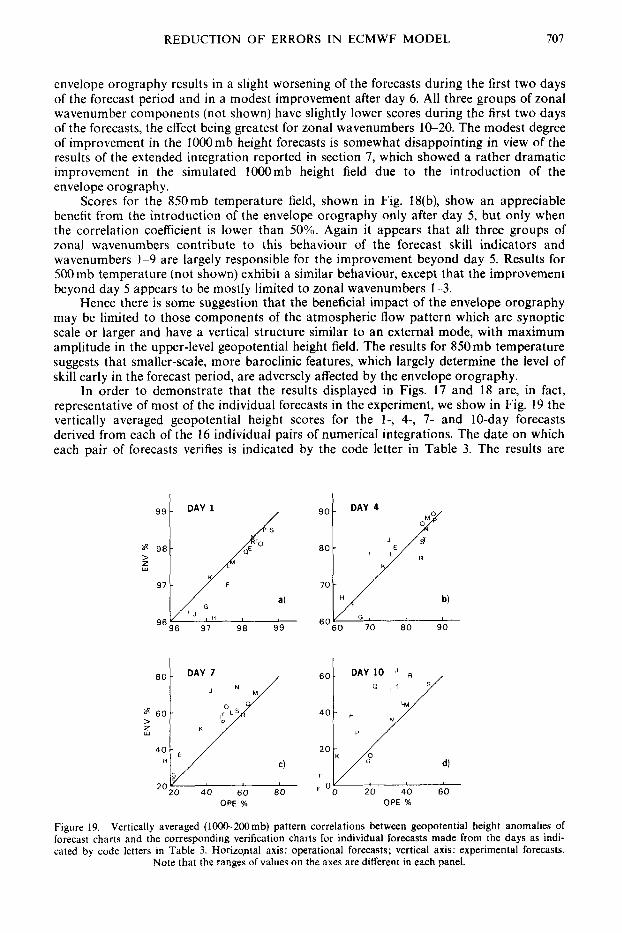
In order to demonstrate that the results displayed in Figs. 17 and 18 are, in fact, representative of most of the individual forecasts in the experiment, we show in Fig. 19 the vertically averaged geopotential height scores for the 1-, 4-, 7- and 10-day forecasts derived from each of the 16 individual pairs of numerical integrations. The date on which each pair of forecasts verifies is indicated by the code letter in Table 3. The results are

DAY 7

80

70 H

40[ H p / F I / E

OPE %

Figure 19. Vertically averaged (1000-200 mb) pattern correlations between geopotential height anomalies of forecast charts and the corresponding verification charts for individual forecasts made from the days as indicated by code letters in Table 3. Horiqntal axis: operational forecasts; vertical axis: experimental forecasts.

Note that the ranges of values on the axes are different in each panel.


piotted in such a way that those letters above the diagonal lines in the respective figures are indicative of a beneficial impact of the envelope orography and vice versa. (Note that the horizontal axes correspond to a different range of scores in each of the four panels.) It is evident from Fig. 19(a) that all but two day 1 operational forecasts are slightly better than their counterparts with the envelope orography. This result is not apparent in the top panel of Fig. 17 because the difference in forecast skill is less than the thickness of the lines in that figure; nevertheless, the differences are large enough to be a cause for concern; for example, if the pattern correlation in a particular forecast drops from 0.98 to 0.976 as a result of the introduction of the envelope orography, it is readily verified that the r.m.s. error increases by almost 10%. By day 4 the scores for the two treatments of the orography are roughly comparable and by days 7 and 10 the envelope orography scores are decisively higher. It is apparent from an inspection of the scores of the individual pairs of forecast integrations (not shown) that there is little if any correlation between the relative (envelope u. operational) performance early in the forecast period and that towards the later part. This behaviour is in accord with the notion that small-scale, highly baroclinic systems largely determine the scores of the short-range forecasts while larger- scale, more barotropic features assume relatively greater importance later on in the forecast period.

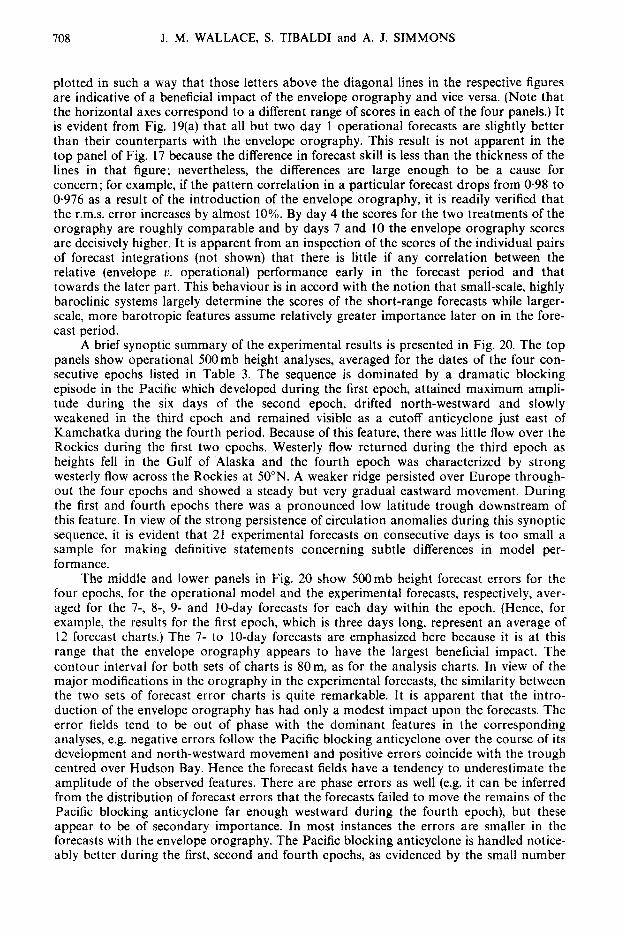
A brief synoptic summary of the experimental results is presented in Fig. 20. The top panels show operational 500mb height analyses, averaged for the dates of the four consecutive epochs listed in Table 3. The sequence is dominated by a dramatic blocking episode in the Pacific which developed during the first epoch, attained maximum amplitude during the six days of the second epoch, drifted north-westward and slowly weakened in the third epoch and remained visible as a cutoff anticyclone just east of Kamchatka during the fourth period. Because of this feature, there was little flow over the Rockies during the first two epochs. Westerly flow returned during the third epoch as heights fell in the Gulf of Alaska and the fourth epoch was characterized by strong westerly flow across the Rockies at 50'". A weaker ridge persisted over Europe throughout the four epochs and showed a steady but very gradual eastward movement. During the first and fourth epochs there was a pronounced low latitude trough downstream of this feature. In view of the strong persistence of circulation anomalies during this synoptic sequence, it is evident that 21 experimental forecasts on consecutive days is too small a sample for making definitive statements concerning subtle differences in model performance.

The middle and lower panels in Fig. 20 show 500mb height forecast errors for the four epochs, for the operational model and the experimental forecasts, respectively, averaged for the 7-, 8-, 9- and 10-day forecasts for each day within the epoch. (Hence, for example, the results for the first epoch, which is three days long, represent an average of 12 forecast charts.) The 7- to 10-day forecasts are emphasized here because it is at this range that the envelope orography appears to have the largest beneficial impact. The contour interval for both sets of charts is 80m, as for the analysis charts. In view of the major modifications in the orography in the experimental forecasts, the similarity between the two sets of forecast error charts is quite remarkable. It is apparent that the introduction of the envelope orography has had only a modest impact upon the forecasts. The error fields tend to be out of phase with the dominant features in the corresponding analyses, e.g. negative errors follow the Pacific blocking anticyclone over the course of its development and north-westward movement and positive errors coincide with the trough centred over Hudson Bay. Hence the forecast fields have a tendency to underestimate the amplitude of the observed features. There are phase errors as well (e.g. it can be inferred from the distribution of forecast errors that the forecasts failed to move the remains of the Pacific blocking anticyclone far enough westward during the fourth epoch), but these appear to be of secondary importance. In most instances the errors are smaller in the forecasts with the envelope orography. The Pacific blocking anticyclone is handled notice- ably better during the first, second and fourth epochs, as evidenced by the small number


of negative contours in its vicinity in the experimental forecasts. The European ridge is handled better during the first two epochs. Many additional examples could be cited and there are few if any glaring counter-examples. Hence the improvements associated with the envelope orography in the later part of the forecast intervals shown in Figs. 17 to 19 apparently involve a reasonably large variety of flow configurations, widely distributed throughout the hemisphere : the impact of the envelope orography on the medium-range forecasts, although modest, appears to have been almost entirely beneficial in this limited sample of wintertime forecasts.

The corresponding results for the 1OOOmb height are shown in Fig. 21, where the contour interval has been halved from that in the previous figure. The error patterns are very similar to those in the 500mb height field and they bear a much more obvious relation to the dominant features on the 500mb charts shown in the previous figure than to those on the corresponding 1OOOmb height charts shown in the top panel of this figure. Hence, for this particular sample of forecasts at least, the skill of the models in the medium range hinges upon their ability to simulate accurately the time evolution of large-scale, low frequency features with a vertical structure similar to that of an external mode.

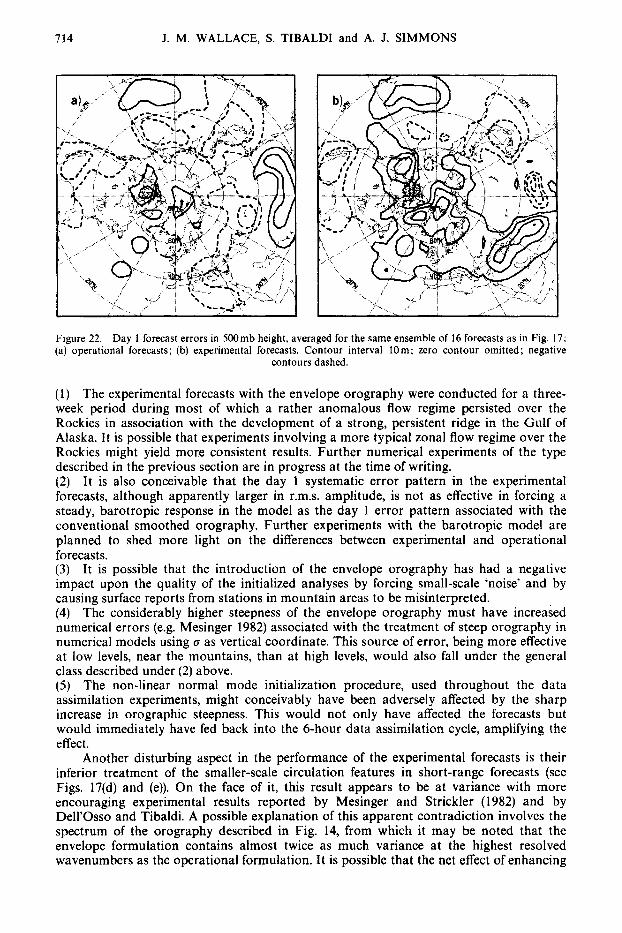
Finally, it is of interest to examine whether the introduction of the envelope orography has resulted in any significant reduction in the day 1 systematic errors, shown in Fig. 22. The patterns for this rather small ensemble of forecasts are rather noisy and therefore it is difficult to draw any definite conclusions. Nevertheless, one gets the distinct impression that the experimental forecasts have somewhat larger errors, particularly over regions of high terrain, where they show a tendency toward positive biases. Examples include the Yukon area in the northern Rockies, Greenland and Afghanistan. Other features, such as the negative biases over Japan and Mexico, were scarcely affected by the introduction of the envelope orography. The prevailing sign of the biases tends to be more positive in the experimental forecasts.

It is evident from the top panels of Fig. 20 that much of the period for which experimental forecasts were made was characterized by a strong ridge over the eastern Pacific, and a northerly wind component over the Rockies. It is only during the fourth epoch that the flow in the vicinity of the Rockies resembled the climatological normal. Hence the comparison in Fig. 22 may not be very representative. A more detailed analysis of systematic errors in the version of the model with the envelope orography will be undertaken in the near future, making use of results of several sets of experiments such as the one described here.

9. DISCUSSION AND CONCLUSIONS

The results in the foregoing sections are mutually consistent in the sense that they support the notion that some kind of enhancement of the smoothed orography, perhaps in the form of an ‘envelope’ increment of the type described in section 6 , may be war- ranted in the formulation of medium- and extended-range numerical weather prediction models and general circulation models. Bleck (1977), Mesinger and Strickler (1982) and Dell’Osso and Tibaldi (1982) reached the same conclusion for short-range numerical prediction models emphasizing regional features such as lee cyclogenesis. Yet there is a glaring contradiction in our results which has not yet been resolved. The original motiva- tion for the forecast experiments described in the previous section was the distinctive and highly reproducible signature in the day 1 forecast error field, with negative biases over the major mountain ranges. Introduction of the envelope orography did not yield the expected reduction of these biases; instead the error pattern was changed in a rather complicated way, with an introduction of even larger positive biases in some regions. However, the enhancement of the orography apparently did have a largely unexpected, beneficial impact upon the medium-range forecasts.

There are several possible explanations for these apparently contradictory results:

Figure 20. Top panels, left to right: 500mb height analyses averaged for the first, second, third and fourth epochs, where the dates for each epoch are listed in Table 3, contour interval 80m. Middle and lower panels: operational and experimental forecast errors, respectively, for SOOmb height for the same four epochs, averaged

for days 7-10, contour interval 80m; negative contours dashed.

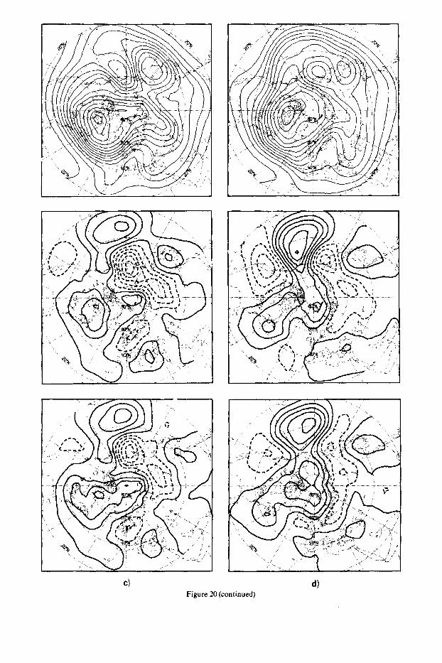
Figure 20 (continued)


Figure 21. As in Fig. 20, but for 1OOOmb height. Contour interval 40m in all panels


Figure 21 (continued)


Figure 22. Day 1 forecast errors in 5OOmb height, averaged for the same ensemble of 16 forecasts as in Fig. 17: (a) operational forecasts; (b) experimental forecasts. Contour interval 10m: zero contour omitted: negative

contours dashed.

(1) The experimental forecasts with the envelope orography were conducted for a three- week period during most of which a rather anomalous flow regime persisted over the Rockies in association with the development of a strong, persistent ridge in the Gulf of Alaska. It is possible that experiments involving a more typical zonal flow regime over the Rockies might yield more consistent results. Further numerical experiments of the type described in the previous section are in progress at the time of writing. (2) It is also conceivable that the day 1 systematic error pattern in the experimental forecasts, although apparently larger in r.m.s. amplitude, is not as effective in forcing a steady, barotropic response in the model as the day 1 error pattern associated with the conventional smoothed orography. Further experiments with the barotropic model are planned to shed more light on the differences between experimental and operational forecasts. (3) It is possible that the introduction of the envelope orography has had a negative impact upon the quality of the initialized analyses by forcing small-scale ‘noise’ and by causing surface reports from stations in mountain areas to be misinterpreted. (4) The considerably higher steepness of the envelope orography must have increased numerical errors (e.g. Mesinger 1982) associated with the treatment of steep orography in numerical models using (i as vertical coordinate. This source of error, being more effective at low levels, near the mountains, than at high levels, would also fall under the general class described under (2) above. ( 5 ) The non-linear normal mode initialization procedure, used throughout the data assimilation experiments, might conceivably have been adversely affected by the sharp increase in orographic steepness. This would not only have affected the forecasts but would immediately have fed back into the 6-hour data assimilation cycle, amplifying the effect.

Another disturbing aspect in the performance of the experimental forecasts is their inferior treatment of the smaller-scale circulation features in short-range forecasts (see Figs. 17(d) and (e)). On the face of it, this result appears to be at variance with more encouraging experimental results reported by Mesinger and Strickler (1982) and by Dell’Osso and Tibaldi. A possible explanation of this apparent contradiction involves the spectrum of the orography described in Fig. 14, from which it may be noted that the envelope formulation contains almost twice as much variance at the highest resolved wavenumbers as the operational formulation. It is possible that the net effect of enhancing


the variance in the higher harmonics of the orography is beneficial in a local sense where an accurate representation of the profile of a particular mountain range is important in simulating the development of a localized synoptic system as in lee cyclogenesis, but harmful in a hemispherically integrated sense because of ‘noise’ associated with the forcing of the higher harmonics which are not adequately resolved with the N48 resolution used in these experiments. Experiments with a more highly smoothed envelope orography are planned to study the influence of the higher harmonics in the orography upon the model performance. Another possible source of error in short-range forecasts and in longer-range forecasts as well, is the improper treatment of the thermal impact of the envelope increment. In the present formulation the observed and calculated surface temperatures are applied at the 0 = 1 level, without regard for the fact that this surface lies not at the average height of the ground, but at the top of the envelope. The distinction may not be too important for high latitude mountain ranges during wintertime, where lapse rates tend to be close to isothermal, but it could contribute to errors in short-range forecasts. The present treatment is almost certain to lead to spurious high-level heat sources over rugged mountain ranges in the tropics and summer hemisphere.

The larger errors in the short-range forecasts inevitably work to the detriment of the performance of the experimental version of the model later on in the forecast interval, and yet beyond day 5 the experimental version of the model seems to perform decisively better than the operational model, at least for this particular sample of forecasts. Apparently the experimental model is more successful in simulating the large-scale, low frequency, equivalent barotropic circulation features which are of crucial importance in medium-range forecasting. Our results indicate that the modelling of these features is moderately sensitive to the prescription of the orography but not overwhelmingly so; despite the superior performance of the experimental model, the error patterns which emerged in experimental and operational forecasts were surprisingly similar. Hence it appears likely that other equally important and potentially remediable sources of error still exist either in the model formulation or in the initialized analyses.

APPENDIX A

THE GLOBAL MEAN HEIGHT ERROR

A component of the systematic forecast error is a global mean lowering of heights which arises from a mean cooling of the model atmosphere. This component has no effect on geostrophic wind errors, and as such cannot be expected to be accurately simulated by the experiments in which the barotropic model is subjected to a forcing derived from day 1 wind errors. Indeed, using the definition of height specified below for the barotropic model, initial experiments in which completely unmodified day 1 errors were used as forcing showed a raising of heights. To compensate for this inadequacy of the barotropic model, a simple modification of the forcing was introduced.

The perturbation height field, h, illustrated in Figs. 6 to 10, is defined from the stream-function, $, which is the basic model variable, by the relation

gh = 2R(sin O)$ (A.1) where g is the acceleration due to gravity, R is the earth’s rotation rate, and 0 is latitude. In the spectral formulation $ is expressed as

1 $: P:(sin O)exp(imA) (‘4.2) the summation being for fml and n < N . 1 is longitude, P: are the associated Legendre functions, and N is a truncation limit. From the orthogonality properties of the Legendre functions, h will have no global mean component if $7 = 0. In view of the perfect angular momentum conserving property of the spectral barotropic model, this can be ensured by adjusting the (): component of the forcing to be zero. Such an adjustment, which has a


negligible effect (through weak non-linearity) on the pattern of response, was carried out for the calculations presented here. Almost equivalently, the contour value separating dashed and solid lines could have been adjusted in the presentation of results to give a distribution of solid and dashed lines more similar to that of the systematic forecast height errors. The alternative use of a fixed reference value of sine, for example 1/42, in (A.l) would also have resulted in no global mean tendency of the model height field.

ACKNOWLEDGMENTS

Many members of the research department of ECMWF are gratefully acknowledged for continuous assistance, stimulus and support. In particular we thank J.-F. Geleyn and R. Striifing for assistance with data handling, J.-F. Louis for assistance with computer graphics, and K. Arpe for assistance with diagnostics and verification packages. The high resolution global orography mentioned throughout was originally produced by the US. Navy and kindly provided by NCAR.

REFERENCES

Bengsson, L. and Lange, A

Blackmon, M. L. and Lau, N.-C.

Bleck, R.

Bolin, B.

Charney, J. G. and Eliassen, A

Cubasch, U.

Dell’Osso, L. and Tibaldi, S.

Derome, J.

Grose, W. L. and Hoskins, B. J.

Held, I.

Hills, T.

Hollingsworth, A., Arpe, K., Tiedtke, M., Capaldo, M. and Savijarvi, R. H.

Hoskins, B. J. and Karoly, D. J.

Kasahara, A. and Washington, W. M.

1982

1980

1977

1950

1949

1981

1982

1981

1979

1983

1979

1980

1981

1969

Manabe, S. and Terpstra, T. B. 1974

Results of the WMOICAS N W P data study and inter- comparison project for forecasts for the Northern Hemi- sphere in 1979-1980. PWPR report, WMO, Geneva.

Regional characteristics of the Northern Hemisphere wintertime circulation: a comparison of the simulation of a GFDL general circulation model with observations. J. Atmos. Sci., 37,497-513.

Numerical simulation of lee cyclogenesis in the Gulf of Genoa. Mon. Wea. Rev., 105, 428-445.

On the influence of the earths orography on the general character of the westerlies. Tellus, 2, 184-195.

A numerical method for predicting the perturbations of the middle latitude westerlies. Telfus, 1, 38-54.

The performance of the ECMWF model in 50 day integrations. ECMWF Tech. Memo. No. 32.

Some preliminary modelling results on an ALPEX case of lee cyclogenesis. ALPEX Preliminary Scientific Results - CARP-ALPEX Report No. 7, WMO, Geneva, 3-19.

On the average errors of an ensemble of forecasts. Atmos.- Ocean, 19, 103-127.

On the influence of orography on the large-scale atmospheric flow. J. Atmos. Sci., 36,223-234.

Stationary and quasi-stationary eddies in the extratropical troposphere: Theory. To appear in Large-scale dynamical processes in the atmosphere, Ed. B. J. Hoskins and R. P. Pearce, Academic Press.

Sensitivity of numerical models to mountain representation. Report of Workshop on Mountains and Numerical Weather Prediction, ECMWF, 20-22 June 1979, 139-161.

The performance of a medium range forecast model in winter - impact of physical parameterisations. Mon. Wea. Rev., 108. 17361773.

The steady linear response of a spherical atmosphere to thermal and orographic forcing. J. Atmos. Sci., 38, 1179- 1 196.

Thermal and dynamical effects of orography on the general circulation of the atmosphere. Proc. WMOjIUGG Symp. Numerical Weather Prediction, Tokyo, Japan Meteorol. Agency, IV, 47-56.

The effects of mountains on the general circulation of the


Mesinger, F.

Mesinger, F. and Strickler, R. F

Pitcher, E. J. P., Malone, R. C., Ramanathan, V., Blackmon, M. L., Puri, K. and Bourke, W.

Simmons, A.J.

Simmons, A. J., Wallace, J. M. and

Tibaldi, S. and Geleyn, J.-F. Branstator, G.

Wallace, J . M. and Woessner, J. K.

1977

1982

1982

1983

1982

1983

1981

1981

atmosphere as identified by numerical experiments. J . Atmos. Sci., 31, 3-42.

Forward-Backward Scheme, and its use in a limited-area model. Beitr. zur Phys. der A m o s . , 50, 200-210.

O n the convergence and error problems of the calculation of the pressure gradient force in sigma coordinate models. Geoph. Astroph. Fluid Dyn., 19, 105-1 17.

Effect of mountains on Genoa Cyclogeneses. Journ. M e t . SOC. Japan, 11, 60, (special issue), 326338.

January and July simulations with a spectral general circulation model. J . Atmos. Sci., 40, 580-604.

The forcing of stationary wave motion by tropical diabatic heating. Quart. J . R. M e t . Soc., 108,503-534.

Barotropic wave propagation and instability, and atmospheric teleconnection patterns. J . Atmos. Sci., in press.

The production of a new orography, land-sea mask and associated climatological surface fields for operational purposes. E C M W F Tech. Memo. No . 40.

An analysis of forecast error in the N M C hemispheric primi- tive equation model. Mon. W e a . Rev., 109, 24462449.

quarterly journal royal meteorological …...quarterly journal of the royal meteorological society...

Documents