Quarterly Beta Forecasting with Multiple Return Frequencies

Anthony R. Barchetto, CFA

tony@saltfinancial.com

Founder and Chief Investment Officer, Salt Financial

April 2018

Traditional estimates of market sensitivity using historical lower-frequency daily or monthly returns

often fail to produce consistently accurate forecasts of near-term beta. We introduce a method that

incorporates higher frequency intraday returns blended with standard daily and monthly return

frequencies that approximates the forecasting accuracy of more complicated long memory models only

using simpler inputs and computation. Calibrated for a one-quarter horizon, the metric is best suited for

managing the level of market-specific risk in constructing or managing portfolios, especially

concentrated at the higher and lower ranges of beta.

2

Introduction

Over 65 years ago, Harry Markowitz (1952) introduced the world to Modern Portfolio Theory (MPT),

discovering the simple but powerful concept that investors seek to optimize return for a given level of

risk. Prior to Markowitz, focus was solely on returns with little emphasis on risk, especially in gauging

how the assets behave together as a portfolio. Markowitz quantified the value of diversification—

spreading your bets—demonstrating that overall portfolio risk can be lower than the weighted average

level of risk in each asset.

Building on Markowitz, William Sharpe (1964) and others developed the simple but elegant Capital Asset

Pricing Model (CAPM) about a decade later. The CAPM established a framework for examining the

trade-off of risk and return. Individual security risk could be “diversified away” by holding a wider

selection of stocks, leaving beta--the sensitivity of the asset to overall market movements—as the sole

factor in the model.

Many investors are familiar with the concept and basic interpretation of beta. A stock with an estimated

beta of 1.0 tends to vary in the same direction and magnitude as the market. A stock with a beta of 1.2

would be expected to vary 20% more than the market (higher volatility); one with a beta of 0.8 would

tend to move 20% less than the market (lower volatility).

All that is required to calculate beta is a series of price returns for the stock and a market proxy such as

the S&P 500. The beta coefficient is an output from a simple linear regression – the slope of the line

created by regressing the returns of the individual stock on the returns of the market. Alternatively,

beta can be calculated as the ratio of how the stock moves with the market (covariance) to the variance

of the market.

In this paper, we will examine several of the traditional methods of estimating beta and introduce a new

method of forecasting called truBeta™, a proprietary process developed by Salt Financial that we believe

to be a more accurate and forward-looking estimate of market risk. We believe a more accurate

forecast of near-term beta—especially for portfolios that are tilted towards either very high or very low

betas—can be a very useful tool for investors to use to construct portfolios and manage risk.

Characteristics of Beta

To begin, it is important to note some of the basic characteristics of beta, most importantly its

limitations as an estimate of future market sensitivity.

1. The choice of interval and timeframe matters greatly

There is no single calculation of beta– it all depends on the series of returns used to generate

the statistic. For example, the most common measure of beta uses five years of monthly

returns for the stock and market index first established by Fama and MacBeth in a 1973 paper

that largely supported the CAPM. But other intervals are also used in practice. Bloomberg uses

two years of weekly returns and applies an adjustment factor to generate its default “Adjusted

Beta” on their market data terminals (more on this later). Others use shorter intervals such as

3

daily returns, often over a trailing one year, to emphasize more recent data in estimating future

beta in the near-term.

The difference between beta calculated using the standard 60 months of returns and one

generated from one year of daily returns can be significant. The table below shows the

differences in beta estimated using monthly versus daily returns as of March 9, 2018 for a

selection of well-known large capitalization stocks. Should an investor expect Microsoft to move

with the market according to its monthly beta of 1.03 or expect more volatility from its daily

estimate of 1.27? Is Disney high beta (1.27 monthly) or low beta (0.77 daily)? Does anyone

believe Netflix has a beta of only 1.09 after a nearly 73% rise in the stock from the end of 2017

through March 9, 2018? These sharp differences make it extremely difficult to properly gauge

how a stock is expected to move with the market over the next month or quarter.

Company Beta (Monthly) Beta (Daily) Difference (Daily-Monthly)

Netflix (NFLX) 1.09 1.58 +0.49

AT&T (T) 0.33 0.78 +0.45

Activision (ATVI) 1.10 1.51 +0.41

Intel (INTC) 0.97 1.31 +0.34

Microsoft (MSFT) 1.03 1.27 +0.24

Merck (MRK) 0.83 0.60 -0.23

Chevron (CVX) 1.14 0.90 -0.24

Coca-Cola (KO) 0.75 0.51 -0.25

Citigroup (C) 1.48 1.18 -0.30

General Motors (GM) 1.57 1.10 -0.47

Sirius XM (SIRI) 1.12 0.64 -0.48

Walt Disney (DIS) 1.27 0.77 -0.50

Amazon.com (AMZN) 1.55 1.04 -0.52

Source: Salt Financial

2. Betas are volatile, even for very large stocks

The CAPM implicitly assumes that betas are relatively stable, but the empirical data show they

are very volatile. Intuitively, this makes sense as fundamentals change, business models evolve

and mature, and growth rates taper off or pick back up according to both internal and external

forces affecting the company.

The chart below shows rolling betas for three of the stocks from above (Microsoft, Disney, and

Chevron), calculated from daily returns (with a 252-day lookback) from March 2013 through

March 2018. Over this five-year period, these three mega-cap stocks—all members of the Dow

Jones Industrial Average—swing back and forth from low to high beta with changes in sector

leadership, macroeconomic factors, and company performance. This makes it extremely

difficult to interpret a beta estimate as a meaningful measure of risk for a given stock.

4

Source: Salt Financial

3. While individual stock betas are noisy, portfolio betas are much more stable

Alexander and Chervany (1980) demonstrate that for portfolios of ten or more securities,

portfolio beta coefficients are much more stable. This also makes sense intuitively, as a basket

of stocks will start to approximate the weighted average beta of the market itself which

mathematically must be 1.0. While the individual components might still be volatile, they will

tend to cancel each other out as beta is a relative measure of volatility. An increase in beta for a

specific stock or sector must be offset somewhere in the market portfolio. In contrast, it is

possible for market volatility in general to be elevated but betas remain constant--the realized

beta for the market is still 1.0 whether volatility is 10% or 30%.

In the sample set of 13 stocks selected above, individual stock betas experience some wild

swings but the portfolio average over the 5-year period is far tamer. Expressed in annualized

terms, the individual stock betas whipped around by an average of 21.7% whereas the portfolio

beta only varied by 5.2%.

Alexander and Chervany also concluded that very high and very low betas, as expressed by the

top and bottom quintiles of the S&P 500 ranked by beta, are far less stable compared to the

middle three quintiles, which will be explored in more detail in the next section.

0.3

0.5

0.7

0.9

1.1

1.3

1.5

Ap

r-1

3

Jul-

13

Oct

-13

Jan

-14

Ap

r-1

4

Jul-

14

Oct

-14

Jan

-15

Ap

r-1

5

Jul-

15

Oct

-15

Jan

-16

Ap

r-1

6

Jul-

16

Oct

-16

Jan

-17

Ap

r-1

7

Jul-

17

Oct

-17

Jan

-18

Rolling Beta - Daily Returns/One Year Lookback

DIS CVX MSFT

5

Introducing truBeta™

Recognizing some of the limitations, we focused on three objectives in designing a new method of

forecasting beta:

• Improve accuracy over traditional historical methods

• Streamline inputs and maintain ease of calculation

• Optimize forecasting performance for the extremes (high/low) instead of the average beta

Accuracy

Using the prior monthly or daily returns to estimate beta are forms of “persistence forecasting”, which is

a fancy way of saying tomorrow will look somewhat like today. The persistence forecast of tomorrow’s

weather using today’s temperatures turns out to be a pretty good forecast. The same forecast used to

project temperatures 10 days from now will be considerably less accurate.1

The core of truBeta™ borrows heavily from techniques developed by academics and refined by

practitioners to forecast near term volatility. The increased availability of higher frequency data to

academic researchers has led to pioneering work on realized volatility from Andersen and Bollerslev

(1998) and Andersen et al. (2001, 2003) and on beta forecasting from Barndorff-Nielsen and Shepherd

(2004), Andersen et al. (2005 and 2006), Hooper et al. (2008), Papageorgiou et al. (2010) and Reeves and

Wu (2013).

A thread common to most of these studies is the use of intraday data in their methodology. While some

might regard this “micro-forecasting” using intraday data as noise, intraday returns have shown to be

useful in gauging near-term volatility. The benefit of using higher frequency data in the analysis is

increased responsiveness to market events. This can also be a detriment if the increased responsiveness

leads to a false short-term signal that “whipsaws” in the other direction, a problem common to any

price-oriented strategy. The key is to temper the responsiveness in the signal to match the investment

horizon to help mitigate rapid reversals.

Most of these studies are calibrated to a one-day horizon, as they are often used in measures like Value

at Risk (VaR), an estimate of the magnitude of expected portfolio losses in a single day in response to

various market shocks. But some are tuned to slightly longer timeframes. Cenesizoglu, Liu, Reeves, and

Wu (2016) demonstrated the efficacy of using intraday data to improve accuracy, using continuous 30-

minute returns to forecast specific levels of beta in a portfolio over a one-month horizon. They show

meaningful improvements in using these intraday returns over more conventional daily and monthly

intervals even for the longer forecast horizon.

truBeta™ uses intraday returns at the heart of its forecast technique but is calibrated to a one-quarter

horizon. The measure is designed for use in portfolio construction to target a specific market risk profile

while limiting turnover. This trades off some accuracy in the very short term for more stability over

intermediate term for situations where constant portfolio adjustments are either impractical or too

costly.

1 “How Accurate Are Weather Forecasts?”, Richard Robbins and Naomi B. Robbins, Huffington Post, 1/29/2015. http://tinyurl.com/y8ovbhmm

6

Ease of Calculation

A number of these studies use sophisticated techniques such as the GARCH (Generalized Autoregressive

Conditional Heteroskedasticity) family of models that more heavily weigh recent observations in the

forecast. However, others use simpler techniques that mimic some of the same dynamics with less

difficulty in computation with substantially similar results. For example, the Heterogeneous

Autoregressive of the Realized Volatility (HAR-RV) model developed by Corsi (2009) uses realized

volatility from three distinct time intervals in a simple OLS regression.

Corsi bases his model on the Heterogeneous Market Hypothesis via Muller et al. (1993), in which market

participants perceive and react to the same information in different ways given different time horizons

and investment objectives. The model uses daily, weekly, and monthly realized volatilities from S&P

futures, USD/CHF rates, and Treasury bond futures from 1989-2003 to forecast one-period (single day)

and multi-period (one week and two week) volatilities in each instrument, demonstrating lower forecast

errors and higher R2 than several alternate GARCH and/or ARMA processes. Most notably, he shows

comparable performance to a more complicated fractionally integrated model (ARFIMA), which is a

“long memory” process in comparison to some of the other models that are strictly “short memory”.

truBeta™ can be best characterized as an adaptation of the HAR-RV framework using some of the inputs

established in the beta forecasting literature, especially the responsiveness of the intraday returns used

by Cenesizoglu et al. (2016). While the Corsi model focuses on realized volatility using log returns, we

substitute beta using simple returns, following precedent in some of the other studies on beta

forecasting. While some details are omitted for competitive reasons, the model is as follows:

𝑡𝑟𝑢𝐵𝑒𝑡𝑎𝑡+60(𝑑)

= 𝑐 + 𝛽(𝑖)𝑅𝐵𝑡(𝑖)

+ 𝛽(𝑑)𝑅𝐵𝑡(𝑑)

+ 𝛽(𝑚)𝑅𝐵𝑡(𝑚)

+ 𝛽(𝑄)𝑄𝑡(𝑑)

+ 𝜖𝑡+60(𝑑)

Where:

𝑅𝐵𝑡(𝑖)

= 𝑖𝑛𝑡𝑟𝑎𝑑𝑎𝑦 𝑟𝑒𝑎𝑙𝑖𝑧𝑒𝑑 𝑏𝑒𝑡𝑎 (𝑝𝑟𝑜𝑝𝑟𝑖𝑒𝑡𝑎𝑟𝑦)

𝑅𝐵𝑡(𝑑)

= 𝑑𝑎𝑖𝑙𝑦 𝑟𝑒𝑎𝑙𝑖𝑧𝑒𝑑 𝑏𝑒𝑡𝑎 (252 𝑑𝑎𝑦𝑠 𝑙𝑜𝑜𝑘𝑏𝑎𝑐𝑘)

𝑅𝐵𝑡(𝑚)

= 𝑚𝑜𝑛𝑡ℎ𝑙𝑦 𝑟𝑒𝑎𝑙𝑖𝑧𝑒𝑑 𝑏𝑒𝑡𝑎 (60 𝑚𝑜𝑛𝑡ℎ 𝑙𝑜𝑜𝑘𝑏𝑎𝑐𝑘)

𝑄𝑡(𝑑)

= 𝑐𝑙𝑎𝑠𝑠𝑖𝑓𝑖𝑐𝑎𝑡𝑖𝑜𝑛 𝑚𝑒𝑡𝑟𝑖𝑐 𝑏𝑎𝑠𝑒𝑑 𝑜𝑛 𝑑𝑎𝑖𝑙𝑦 𝑟𝑒𝑎𝑙𝑖𝑧𝑒𝑑 𝑏𝑒𝑡𝑎 (𝑝𝑟𝑜𝑝𝑟𝑖𝑒𝑡𝑎𝑟𝑦)

Optimization

In lieu of a simple OLS regression, we used Microsoft’s Azure Machine Learning Studio to train a

regression model using one of the more sophisticated algorithms available on the platform. We used

over 14,000 quarterly observations using large and mid-cap stocks, splitting the data into a training set

of 65%, leaving the rest for the validation dataset. The model was optimized to minimize mean absolute

error between forecasted and predicted values.

The benefit of using the Azure platform is the ease of configuration using very powerful tools and a

robust API for use in production. The downside is a lack of more common regression statistics such as

7

confidence intervals to gauge statistical significance, although alternate measures are provided to better

understand the impact and importance of each feature added to the model.

Machine learning is somewhat over-hyped lately, but our use of the technique in this model is very

measured and deliberate. Using just the intraday realized beta alone resulted in a more accurate

forecast than the traditional measures. But the machine learning process was able to further improve

MAE by 9.5% and MSE by 15.8%. More importantly, it was able to use the lower frequency return

calculations to more effectively forecast the very high and low betas, meeting our third objective and

giving truBeta™ what we consider to be a clearer advantage over more traditional methods. It corrected

the over- and under-estimation of more extreme betas while managing to keep some of the potentially

false signals influenced by the increased responsiveness of the intraday beta component under control.

Data and Methodology

The data for this analysis are collected from several sources. The Solactive US Large and Midcap Index

consisting of the top 1000 free-float market capitalization weighted US stocks (similar in construction to

the Russell 1000 Large Cap Index) was selected as the stock universe. Price data on these securities

from 2004-2017 was provided by Cboe’s Livevol DataShop (intraday bars), Xignite (daily and monthly

returns), and Bloomberg (adjusted close prices). Sector classifications, where necessary, were provided

by FactSet’s RBICS.

The data were analyzed at each quarterly rebalancing of the index (the second Friday of March, June,

September, and December) to maintain consistency with the selected universe. The following ex-ante

betas were computed at each quarterly rebalance as follows:

• Monthly – monthly returns for the prior 60 months (5 years)

• Daily – daily returns for the prior 252 days (1 year)

• Bloomberg Adjusted – weekly returns for the prior 104 weeks (2 years), adjusted by multiplying

the “raw” calculation by 0.67 and then adding 0.332

• truBeta™ – Salt’s proprietary forecast that blends monthly, daily, and intraday returns with the

help of a machine learning algorithm trained on 14 years of historical data

To compute ex-post (realized) betas to measure accuracy over the next quarter (closing price 60 trading

days later), the daily/1-year interval was chosen as an appropriate benchmark balanced between the

longer dated monthly and Bloomberg calculations and the truBeta™ forecast, which uses intraday data

in its calculation.

All observations with missing price or beta calculations (due to symbology issues, data availability, etc.)

were dropped, reducing total observations by 2.5% to 53,641. To reduce the impact of suspiciously high

or low betas over a relatively small number of observations (60 days), all observations with a beta

forecast (in any method) or realized beta equal to or above 5.00 or equal to or less than -5.00 were

discarded, leaving 53,500 observations.

2 This heuristic mathematically pulls all raw beta estimates towards 1.0. Bloomberg allows users to modify the standard parameters to calculate beta but the 2 years of weekly returns is the default.

8

As individual betas are very noisy, portfolio betas were used for comparison. The data were sliced into

deciles by level of daily historical beta at each period. Each decile of approximately 100 stocks was

analyzed as an equal-weighted portfolio, comparing the simple average of each portfolio beta forecast

at the rebalancing date to the average portfolio ex-post beta at the end of the 60-day period. The data

were aggregated by method (Monthly, Daily, etc.) and then by decile to calculate the following statistics:

• Average Error – mean difference between the forecast value and realized, including the sign

• Mean Absolute Error (MAE) – mean difference of the absolute value of forecast minus realized

• Mean Squared Error (MSE) – the mean difference between forecast and realized, squared

By Decile- Overall Average Error MAE MSE

Monthly 0.0470 0.1617 0.0481 Daily 0.0037 0.1394 0.0388

Bloomberg Adjusted 0.0001 0.1284 0.0320 truBeta™ -0.0512 0.1125 0.0229

Source: Salt Financial

The data show accuracy improving (both MAE and MSE) in moving from Monthly to Daily returns. The

Bloomberg Adjusted estimate, which uses weekly returns, are superior to both, owing much to the

adjustment factor pulling both high and low betas closer to one despite the use of a longer historical

look-back than Daily. But the truBeta™ forecast dominates all three with the lowest MAE (0.1125) and

MSE (the metric that punishes outlier errors more severely) 52% better than Monthly, 41% better than

Daily, and 28% better than Bloomberg Adjusted.

In terms of bias, the Bloomberg Adjusted estimate proved to be the least biased estimator with a near

zero average error and the Daily estimate next best at 0.0037. The Monthly estimate showed a

significant positive bias whereas truBeta™ was biased to the downside. Since the Bloomberg Adjusted

metric mathematically forces the raw historical calculation closer to 1.0 (by multiplying by 0.67 and then

adding 0.33 to the raw calculation), it should be no surprise that its errors added up closest to zero.

The data get more interesting when looking into the decile groupings. The chart below shows average

error by method in each decile.

9

Source: Salt Financial

Of note is the large overestimation in the higher deciles in the Monthly and Daily forecasts. The average

error for the highest beta decile for both is over 0.20, indicating a very strong upward bias. On the other

side, a bias to the downside for the lowest betas is more pronounced for the Daily estimate than

Monthly, but the slope of the line is positive for both as beta moves from lower to higher deciles. The

Bloomberg Adjusted estimate over-corrects at both the high and low end (more severely at the low end)

with a clearly negative slope from low to high deciles.

While the overall statistics favor the Bloomberg Adjusted and Daily forecasts as the least biased

estimators, a closer look at the distribution reveals that the larger errors at the extremes almost

completely cancel each other out, masking the large bias at the extremes. These findings are consistent

with other studies analyzing realized vs. forecast beta using lower-frequency interval returns such as

daily or monthly in deciles or quintiles that show downward bias in the lower ranges and upward bias in

the higher (Vasicek, 1973). truBeta™ maintains a consistent slight negative bias to the downside across

all deciles, most notably in the higher beta ranges (deciles 8-10), with an average of -0.0519, very close

to its overall average of -0.0512.

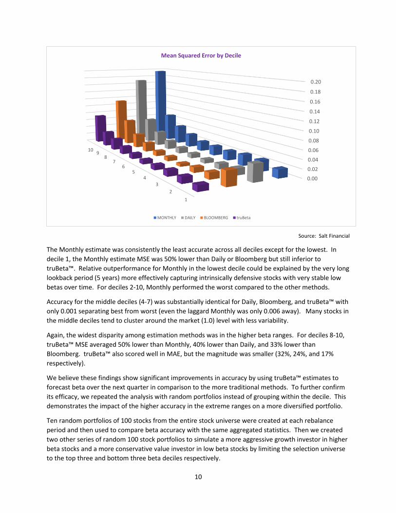
truBeta™ forecasts were also significantly more accurate in terms of MAE and MSE at the extremes.

Since results for both metrics were substantial similar in respect to the ranking of each method, we will

focus on MSE in the graph below to better highlight the impact of outsized errors for each forecast

model.

-0.20

-0.15

-0.10

-0.05

0.00

0.05

0.10

0.15

0.20

0.25

1 2 3 4 5 6 7 8 9 10

Deciles (Based on 1 Year/Daily Return Historical Beta)

Average Forecast Error by Historical Beta Decile

MONTHLY DAILY BLOOMBERG truBeta

10

Source: Salt Financial

The Monthly estimate was consistently the least accurate across all deciles except for the lowest. In

decile 1, the Monthly estimate MSE was 50% lower than Daily or Bloomberg but still inferior to

truBeta™. Relative outperformance for Monthly in the lowest decile could be explained by the very long

lookback period (5 years) more effectively capturing intrinsically defensive stocks with very stable low

betas over time. For deciles 2-10, Monthly performed the worst compared to the other methods.

Accuracy for the middle deciles (4-7) was substantially identical for Daily, Bloomberg, and truBeta™ with

only 0.001 separating best from worst (even the laggard Monthly was only 0.006 away). Many stocks in

the middle deciles tend to cluster around the market (1.0) level with less variability.

Again, the widest disparity among estimation methods was in the higher beta ranges. For deciles 8-10,

truBeta™ MSE averaged 50% lower than Monthly, 40% lower than Daily, and 33% lower than

Bloomberg. truBeta™ also scored well in MAE, but the magnitude was smaller (32%, 24%, and 17%

respectively).

We believe these findings show significant improvements in accuracy by using truBeta™ estimates to

forecast beta over the next quarter in comparison to the more traditional methods. To further confirm

its efficacy, we repeated the analysis with random portfolios instead of grouping within the decile. This

demonstrates the impact of the higher accuracy in the extreme ranges on a more diversified portfolio.

Ten random portfolios of 100 stocks from the entire stock universe were created at each rebalance

period and then used to compare beta accuracy with the same aggregated statistics. Then we created

two other series of random 100 stock portfolios to simulate a more aggressive growth investor in higher

beta stocks and a more conservative value investor in low beta stocks by limiting the selection universe

to the top three and bottom three beta deciles respectively.

0.00

0.02

0.04

0.06

0.08

0.10

0.12

0.14

0.16

0.18

0.20

1

2

3

45

67

89

10

Mean Squared Error by Decile

MONTHLY DAILY BLOOMBERG truBeta

11

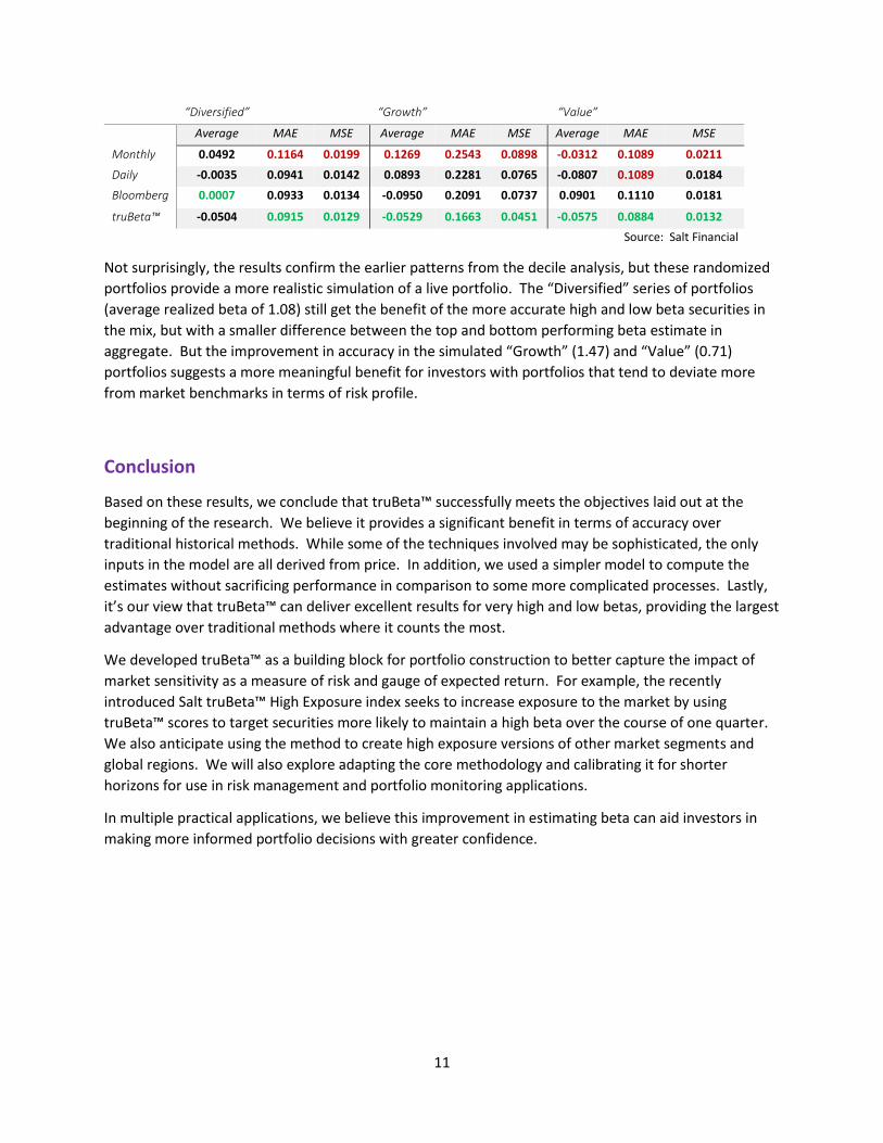
“Diversified” “Growth” “Value”

Average MAE MSE Average MAE MSE Average MAE MSE

Monthly 0.0492 0.1164 0.0199 0.1269 0.2543 0.0898 -0.0312 0.1089 0.0211

Daily -0.0035 0.0941 0.0142 0.0893 0.2281 0.0765 -0.0807 0.1089 0.0184

Bloomberg 0.0007 0.0933 0.0134 -0.0950 0.2091 0.0737 0.0901 0.1110 0.0181

truBeta™ -0.0504 0.0915 0.0129 -0.0529 0.1663 0.0451 -0.0575 0.0884 0.0132

Source: Salt Financial

Not surprisingly, the results confirm the earlier patterns from the decile analysis, but these randomized

portfolios provide a more realistic simulation of a live portfolio. The “Diversified” series of portfolios

(average realized beta of 1.08) still get the benefit of the more accurate high and low beta securities in

the mix, but with a smaller difference between the top and bottom performing beta estimate in

aggregate. But the improvement in accuracy in the simulated “Growth” (1.47) and “Value” (0.71)

portfolios suggests a more meaningful benefit for investors with portfolios that tend to deviate more

from market benchmarks in terms of risk profile.

Conclusion

Based on these results, we conclude that truBeta™ successfully meets the objectives laid out at the

beginning of the research. We believe it provides a significant benefit in terms of accuracy over

traditional historical methods. While some of the techniques involved may be sophisticated, the only

inputs in the model are all derived from price. In addition, we used a simpler model to compute the

estimates without sacrificing performance in comparison to some more complicated processes. Lastly,

it’s our view that truBeta™ can deliver excellent results for very high and low betas, providing the largest

advantage over traditional methods where it counts the most.

We developed truBeta™ as a building block for portfolio construction to better capture the impact of

market sensitivity as a measure of risk and gauge of expected return. For example, the recently

introduced Salt truBeta™ High Exposure index seeks to increase exposure to the market by using

truBeta™ scores to target securities more likely to maintain a high beta over the course of one quarter.

We also anticipate using the method to create high exposure versions of other market segments and

global regions. We will also explore adapting the core methodology and calibrating it for shorter

horizons for use in risk management and portfolio monitoring applications.

In multiple practical applications, we believe this improvement in estimating beta can aid investors in

making more informed portfolio decisions with greater confidence.

12

Appendix A – Forecasting Accuracy by Decile

Mean Absolute Error (MAE)

1 2 3 4 5 6 7 8 9 10

MONTHLY 0.1115 0.1144 0.1159 0.1145 0.1246 0.1307 0.1505 0.1710 0.2223 0.3612

DAILY 0.1627 0.0974 0.0841 0.0786 0.0798 0.0931 0.1112 0.1420 0.2036 0.3413

BLOOMBERG 0.1571 0.1019 0.0812 0.0647 0.0748 0.0856 0.1180 0.1482 0.1917 0.2603

truBeta 0.0888 0.0926 0.0870 0.0855 0.0786 0.0881 0.1084 0.1289 0.1501 0.2173

Mean Squared Error (MSE)

1 2 3 4 5 6 7 8 9 10

MONTHLY 0.0193 0.0256 0.0255 0.0219 0.0224 0.0233 0.0326 0.0459 0.0693 0.1950

DAILY 0.0392 0.0158 0.0122 0.0092 0.0106 0.0139 0.0205 0.0351 0.0616 0.1696

BLOOMBERG 0.0335 0.0150 0.0121 0.0067 0.0097 0.0117 0.0217 0.0340 0.0631 0.1121

truBeta 0.0134 0.0145 0.0138 0.0112 0.0099 0.0124 0.0180 0.0273 0.0360 0.0729

Results represent quarterly measurement of accuracy of four beta forecasting methods using

components of the Solactive US Large and Midcap Index from March 2004 through December 2017.

13

References

Alexander, Gordon J., Chervany, Norman L., “On the Estimation and Stability of Beta”, Journal of Financial and Quantitative Analysis, 15(01) (March 1980) 123-137. Andersen, T.G., Bollerslev, T., “Answering the Skeptics: Yes. Standard Volatility Models Do Provide Accurate Forecasts”, International Economic Review 39 (1998), 885-905. Andersen, T. G., Bollerslev, T., Diebold, F. X., Ebens. H., “The Distribution of Realized Stock Return Volatility”, Journal of Financial Economics 61 (2001a), 43-67. Andersen, T. G., Bollerslev, T., Diebold, F. X., Labys., P., “The Distribution of Exchange Rate Volatility”, Journal of the American Statistical Association 96 (2001b), 42-55. Andersen, T.G., Bollerslev, T., Diebold, F.X., Labys, P., “Modeling and Forecasting Realized Volatility. Econometrica 71 (2003), 529-626. Andersen, T.G., Bollerslev, T., Diebold, F.X., Wu G., “A Framework for Exploring the Macroeconomic Determinants of Systematic Risk”, American Economic Review 95 (2005), 398-404. Barndorff-Nielsen, O.E., Shephard, N., “Econometric Analysis of Realised Covariation: High Frequency Based Covariance, Regression and Correlation in Financial Economics”, Econometrica 72 (2004), 885-925. Cenesizoglu, T., Liu, Q., Reeves, J.J., Wu, H., “Monthly Beta Forecasting with Low-, Medium- and High-Frequency Stock Returns”, The Journal of Forecasting, Volume 35, Issue 6 (Sep 2016) 528-541. Corsi, Fulvio, “A Simple Approximate Long-Memory Model of Realized Volatility”, The Journal of Financial Econometrics, Vol. 7, No. 2 (2009) 174–196. Fama, Eugene F., MacBeth, James D., “Risk, Return, and Equilibrium: Empirical Tests”, The Journal of Political

Economy, Vol 81., No 3 (May-Jun 1973) 607-636.

Hooper, V.J., Ng, K., Reeves, J.J. “Quarterly Beta Forecasting: An Evaluation”, International Journal of Forecasting 24 (2008), 480-489. Markowitz, Harry, “Portfolio Selection”, The Journal of Finance, Vol 7, No.1 (Mar 1952), 77-91. Muller, U., M. Dacorogna, R. Dav, O. Pictet, R. Olsen, and J. Ward. 1993. “Fractals and Intrinsic Time – A challenge to econometricians”, 39th International AEA Conference on Real Time Econometrics, (14–15 October 1993), Luxembourg Papageorgiou, N., Reeves, J.J., Xie, X., “Betas and the Myth of Market Neutrality”, Working Paper, Australian School of Business, University of New South Wales (2010). Reeves, J.J., Wu, H., “Constant vs. Time-varying Beta Models: Further Forecast Evaluation”, Journal of Forecasting 32 (2013), 256-266. Sharpe, William F., “Capital Asset Prices: A Theory of Market Equilibrium under Conditions of Risk”, The Journal of

Finance, Vol 19., No 3 (Sep 1964).

Vasicek, Oldrich A., “A Note on Using Cross-Sectional Information in Bayesian Estimation of Security Betas”, The Journal of Finance, vol. 28, No. 5 (December 1973) 1233-1239.

14

Disclosures

©2018 Salt Financial LLC is a registered investment adviser. The information provided herein is for

information purposes only and is not intended to be and does not constitute financial, investment, tax or

legal advice. Investment advice can be provided only after a properly executed investment advisory

agreement has been entered into by the client and Salt Financial LLC (“Salt”). All investments are subject

to risks, including the risk of loss of principal. Past performance is not an indicator of future results.

The information and opinions contained in Salt's blog posts, market commentaries and other writings are

of a general nature and are provided solely for the use of Salt, its clients and prospective clients. This

content is not to be reproduced, copied or made available to others without the expressed written

consent of Salt. These materials reflect the opinion of Salt on the date of production and are subject to

change at any time without notice. Due to various factors, including changing market conditions or tax

laws, the content may no longer be reflective of current opinions or positions.

Any market observations and data provided are for informational purposes only. Where data is

presented that is prepared by third parties, such information will be cited, and these sources have been

deemed to be reliable. However, Salt does not warrant the accuracy of this information. Salt and any

third parties listed, cited or otherwise identified herein are separate and unaffiliated and are not

responsible for each other’s policies, products or services.