Quantum spectral analysis: frequency in time,

with applications to signal and image processing.

Mario Mastriani

Quantum Communications Division, Merx Communications LLC, 2875 NE 191 st, suite 801, Aventura, FL 33180, USA

mmastri@merxcomm.com

Abstract A quantum time-dependent spectrum analysis, or simply, quantum spectral analysis (QSA) is

presented in this work, and it’s based on Schrödinger equation, which is a partial differential equation that

describes how the quantum state of a non-relativistic physical system changes with time. In classic world is

named frequency in time (FIT), which is presented here in opposition and as a complement of traditional

spectral analysis frequency-dependent based on Fourier theory. Besides, FIT is a metric, which assesses the

impact of the flanks of a signal on its frequency spectrum, which is not taken into account by Fourier theory

and even less in real time. Even more, and unlike all derived tools from Fourier Theory (i.e., continuous,

discrete, fast, short-time, fractional and quantum Fourier Transform, as well as, Gabor) FIT has the following

advantages: a) compact support with excellent energy output treatment, b) low computational cost, O(N) for

signals and O(N2) for images, c) it does not have phase uncertainties (indeterminate phase for magnitude = 0)

as Discrete and Fast Fourier Transform (DFT, FFT, respectively), d) among others. In fact, FIT constitutes

one side of a triangle (which from now on is closed) and it consists of the original signal in time, spectral

analysis based on Fourier Theory and FIT. Thus a toolbox is completed, which it is essential for all

applications of Digital Signal Processing (DSP) and Digital Image Processing (DIP); and, even, in the latter,

FIT allows edge detection (which is called flank detection in case of signals), denoising, despeckling,

compression, and superresolution of still images. Such applications include signals intelligence and imagery

intelligence. On the other hand, we will present other DIP tools, which are also derived from the Schrödinger

equation. Besides, we discuss several examples for spectral analysis, edge detection, denoising, despeckling,

compression and superresolution in a set of experimental results in an important section on Applications and

Simulations, respectively. Finally, we finish this work with special section dedicated to Conclusions.

Keywords Compression • Denoising • Despeckling • Digital Signal and Image Processing • Edge Detection

• Fourier Theory • Imagery Intelligence • Quantum Information Processing • Schrödinger equation • Signals

Intelligence • Spectral Analysis • Superresolution of still images • Wavelets.

1 Introduction

Quantum computation and quantum information is the study of the information processing tasks that can be

accomplished using quantum mechanical systems. Like many simple but profound ideas it was a long time

before anybody thought of doing information processing using quantum mechanical systems [1].

Quantum computation is the field that investigates the computational power and other properties of

computers based on quantum-mechanical principles. An important objective is to find quantum algorithms

that are significantly faster than any classical algorithm solving the same problem. The field started in the

early 1980s with suggestions for analog quantum computers by Paul Benioff [2] and Richard Feynman [3,

4], and reached more digital ground when in 1985 David Deutsch defined the universal quantum Turing

machine [5]. The following years saw only sparse activity, notably the development of the first algorithms by

Deutsch and Jozsa [6] and by Simon [7], and the development of quantum complexity theory by Bernstein

and Vazirani [8]. However, interest in the field increased tremendously after Peter Shor’s very surprising

discovery of efficient quantum algorithms (or simulations on a quantum computer) for the problems of

integer factorization and discrete logarithms in 1994 [9].

Quantum Information Processing (QIP) - The main concepts related to Quantum Information Processing

may be grouped in the next topics: quantum bit (qubit, which is the elemental quantum information unity),

Bloch’s Sphere (geometric environment for qubit representation), Hilbert’s Space (which generalizes the

notion of Euclidean space), Schrödinger’s Equation (which is a partial differential equation that describes

how the quantum state of a physical system changes with time.), Unitary Operators, Quantum Circuits (in

quantum information theory, a quantum circuit is a model for quantum computation in which a computation

is a sequence of quantum gates, which are reversible transformations on a quantum mechanical analog of an

n-bit register. This analogous structure is referred to as an n-qubit register.), Quantum Gates (in quantum

computing and specifically the quantum circuit model of computation, a quantum gate or quantum logic gate

is a basic quantum circuit operating on a small number of qubits), and Quantum Algorithms (in quantum

computing, a quantum algorithm is an algorithm which runs on a realistic model of quantum computation,

the most commonly used model being the quantum circuit model of computation) [1, 10-12].

Nowadays, other concepts complement our knowledge about QIP, they are:

Quantum Signal Processing (QSP) - The main idea is to take a classical signal, sample it, quantify it (for

example, between 0 and 255), use a classical-to-quantum interface, give an internal representation to that

signal, make a processing to that quantum signal (denoising, compression, among others), measure the result,

use a quantum-to-classical interface and subsequently detect the classical outcome signal. Interestingly, and

as will be seen later, the quantum image processing has aroused more interest than QSP. In the words of its

creator: “many new classes of signal processing algorithms have been developed by emulating the behavior

of physical systems. There are also many examples in the signal processing literature in which new classes of

algorithms have been developed by artificially imposing physical constraints on implementations that are not

inherently subject to these constraints”. Therefore, Quantum Signal Processing (QSP) is a signal processing

framework [13, 14] that is aimed at developing new or modifying existing signal processing algorithms by

borrowing from the principles of quantum mechanics and some of its interesting axioms and constraints.

However, in contrast to such fields as quantum computing and quantum information theory, it does not

inherently depend on the physics associated with quantum mechanics. Consequently, in developing the QSP

framework we are free to impose quantum mechanical constraints that we find useful and to avoid those that

are not. This framework provides a unifying conceptual structure for a variety of traditional processing

techniques and a precise mathematical setting for developing generalizations and extensions of algorithms,

leading to a potentially useful paradigm for signal processing with applications in areas including frame

theory, quantization and sampling methods, detection, parameter estimation, covariance shaping, and

multiuser wireless communication systems.” The truth is that to date, papers on this discipline are less than

half a dozen, and its practical use is practically nil. Moreover, although it is an interesting idea, developed so

far, does not withstand further comment.

Quantum Image Processing (QImP) - it is a young discipline and it is in training now, however, it’s much

more developed than QSP. QImP starts in 1997. That year, Vlasov proposed a method of using quantum

computation to recognize so-called orthogonal images [15]. Five years later, in 2002, Schutzhold described a

quantum algorithm that searches specific patterns in binary images [16]. A year later, in October 2003,

Beach, Lomont, and Cohen from Cybernet Systems Corporation, (an organization with a close cooperative

relationship with the US Defense Department) demonstrated the possibility that quantum algorithms (such as

Grover’s algorithm) can be used in image processing. In that paper, they describe a method which uses a

quantum algorithm to detect the posture of certain targets. Their study implies that quantum image

processing may, in future, play a valuable role during wartime [17].

Later, we can found the works of Venegas-Andraca [18], where he proposes quantum image representations

such as Qubit Lattice [19, 20]; in fact, this is the first doctoral thesis in the specialty, The history continues

with the quantum image representation via the Real Ket [21] of Latorre Sentís, with a special interest in

image compression in a quantum context. A new stage begins with the proposal of Le et al. [22], for a

flexible representation of quantum images to provide a representation for images on quantum computers in

the form of a normalized state which captures information about colors and their corresponding positions in

the images. History continues up to date by different authors and their innovative internal representation

techniques of the image [23-44].

Very similar to the case of QSP, the idea in back of QImP is to take a classic image (captured by a digital

camera or photon counter) and place it in a quantum machine through a classical-to-quantum interface, give

some internal representation to the image using the procedures mentioned above, perform processing on it

(denoising, compression, among others), measure the results, restore the image through another interface but

this time quantum-classical, y ready. The contribution of a quantum machine over a classic machine when it

comes to process images it is that the former has much more power of processing. This last advantage can

handle images and algorithms of a high computational cost, which would be unmanageable in a classic

machine in a practical sense.

The problem of this discipline lies in its genetic, given that QImP is the daughter of Quantum Information

Processing and Digital Image Processing, thus, we fall into the old dilemma of teaching, i.e.: to teach Latin

to Peter, we should know more about Latin and more about Peter? The answer is simple: we should know

very well of both, but the mission becomes impossible. In other words, what is acceptable in Quantum

Information Processing, and (at the same time) inadmissible in Digital Image Processing?

The mentioned problem begins with the quantum measurement, then, if after processing the image within the

quantum computer, we want to retrieve the result by tomography of quantum states, we will encounter a

serious obstacle, this is:

if we make a tomography of quantum states in Quantum Information Processing (even, this can be extended

to any method of quantum measurement after the tomography) with an error of 6% in our knowledge of the

state, this constitutes an excellent measure of such state, but on the other hand, and this time from the

standpoint of Digital Image Processing [45-48], an error of 6 % in each pixel of the outcome image

constitutes a disaster, since this error becomes unmanageable and exaggerated noise. So overwhelming is

the aforementioned disaster that the recovered image loses its visual intelligibility, i.e., its look and feel, and

morphology, due to the destruction of edges and textures.

This speaks clearly (and for this purpose, one need only read the papers of QImP cited above) that these

works are based on computer simulations in classical machines, exclusively (in most cases in MATLAB®

[49]), and do not represent test in a laboratory of Quantum Physics. In fact, if these field trials were held, the

result would be the aforementioned. We just have to go to the lab and try with a single pixel of an image,

then extrapolate the results to the entire image and therefore the inconvenience will be explicit. On the other

hand, today there are obvious difficulties to treat a full image inside a quantum machine, however, there is no

difficulty for a single pixel, since that pixel represents a single qubit, and this can be tested in any laboratory

in the world, without problems. Therefore, there are no excuses.

Definitely, the problem lies in the hostile relationship between the internal representation of the image

(inside quantum machine), the outcome measurement, and the recovery of the image outside of quantum

machine. Therefore, the only technique of QImP that survives is QuBoIP [50]. This is because it works with

CBS, exclusively, and the quantum measurement does not affect the value of states. However, it is important

to clarify that both, i.e., traditional techniques QImP and QuBoIP share a common enemy, and this is the

decoherence [1, 50].

Quantum Cryptography - Since most of current classical cryptography is based on the assumption that these

two problems are computationally hard, the ability to actually build and use a quantum computer would

allow us to break most current classical cryptographic systems, notably the Rivest, Shamir y Adleman (RSA)

system [51, 52]. In contrast, a quantum form of cryptography due to Bennett and Brassard [53] is

unbreakable even for quantum computers. Besides, Quantum cryptography is the synthesis of quantum

mechanics with the art of code-making (cryptography) [54]. The idea was first conceived in an unpublished

manuscript written by Stephen Wiesner around 1970 [55]. However, the subject received little attention until

its resurrection by a classic paper published by Bennett and Brassard in 1984 [53]. The goal of quantum

cryptography is to perform tasks that are impossible or intractable with conventional cryptography. Quantum

cryptography makes use of the subtle properties of quantum mechanics such as the quantum no-cloning

theorem and the Heisenberg uncertainty principle. Unlike conventional cryptography, whose security is often

based on unproven computational assumptions, quantum cryptography has an important advantage in that its

security is often based on the laws of physics. Thus far, proposed applications of quantum cryptography

include quantum key distribution (abbreviated QKD), quantum bit commitment and quantum coin tossing.

These applications have varying degrees of success. The most successful and important application—

QKD—has been proven to be unconditionally secure. Moreover, experimental QKD has now been

performed over hundreds of kilometers over both standard commercial telecom optical fibers and open-air.

In fact, commercial QKD systems are currently available on the market.

On a wider context, quantum cryptography is a branch of quantum information processing, which includes

quantum computing, quantum measurements, and quantum teleportation. Among all branches, quantum

cryptography is the branch that is closest to real-life applications. Therefore, it can be a concrete avenue for

the demonstrations of concepts in quantum information processing. On a more fundamental level, quantum

cryptography is deeply related to the foundations of quantum mechanics, particularly the testing of Bell-

inequalities and the detection efficiency loophole. On a technological level, quantum cryptography is related

to technologies such as single-photon measurements and detection and single-photon sources.

Quantum Technology - Quantum technology is a new field of physics and engineering, which transitions

some of the stranger features of quantum mechanics, especially quantum entanglement and most recently

quantum tunneling, into practical applications such as quantum computing, quantum cryptography, quantum

simulation, quantum metrology, quantum sensing, and quantum imaging.

The field of quantum technology was first outlined in a 1997 book by Gerard J. Milburn [56], which was

then followed by a 2003 article by Jonathan P. Dowling and Gerard J. Milburn [57, 58], as well as a 2003

article by David Deutsch [59]. The field of quantum technology has benefited immensely from the influx of

new ideas from the field of quantum information processing, particularly quantum computing. Disparate

areas of quantum physics, such as quantum optics, atom optics, quantum electronics, and quantum

nanomechanical devices, have been unified under the search for a quantum computer and given a common

language, that of quantum information theory. In actuality, the most outstanding works in this area belong to

Cappelaro's group at MIT [60-63].

Quantum Fourier Transform (QFT) - In quantum computing, the QFT is a linear transformation on

quantum bits and is the quantum analogue of the discrete Fourier transform. The QFT is a part of many

quantum algorithms, notably Shor's algorithm for factoring and computing the discrete logarithm, the

quantum phase estimation algorithm for estimating the eigenvalues of a unitary operator, and algorithms for

the hidden subgroup problem.

The QFT can be performed efficiently on a quantum computer, with a particular decomposition into a

product of simpler unitary matrices. Using a simple decomposition, the discrete Fourier transform can be

implemented as a quantum circuit consisting of only O(n2) Hadamard gates and controlled phase shift gates,

where n is the number of qubits [1]. This can be compared with the classical discrete Fourier transform,

which takes O(2n2) gates (where n is the number of bits), which is exponentially more than O(n2). However,

the quantum Fourier transform acts on a quantum state, whereas the classical Fourier transform acts on a

vector, so not every task that uses the classical Fourier transform can take advantage of this exponential

speedup. The best QFT algorithms known today require only O(n log n) gates to achieve an efficient

approximation [64].

Quantum Information Theory (QIT) - QIT is motivated by the study of communications channels, but it has

a much wider domain of application, and it is a thought-provoking challenge to capture in a verbal nutshell

the goals of the field. QIT is fundamentally richer than classical information theory, because quantum

mechanics includes so many more elementary classes of static and dynamic resources – not only does it

support all the familiar classical types, but there are entirely new classes such as the static resource of

entanglement to make life even more interesting than it is classically [1].

QIT deals with four main topics [65]:

- Transmission of classical information over quantum channels.

- The tradeoff between acquisition of information about a quantum state and disturbance of the state.

- Quantifying quantum entanglement.

- Transmission of quantum information over quantum channels.

For which, it involves four components:

- Quantum Entropy [1]: In QIT, we can talk of: quantum relative entropy, the von Neumann entropy, the

joint quantum entropy, and the conditional quantum entropy,

- Quantum Channel [66],

- Quantum Cryptography (aforementioned), and

- Quantum Compression [1, 67-71].

Finally, this work is organized as follows: Prolegomenous to QSA are outlined in Section 2, where, we

present the follow concepts: continuous, discrete, fast, short-time (including Gabor transform), and fractional

Fourier transform, wavelets and multirresolution, smoothing of coefficients in wavelet domain in 1D and 2D,

superresolution with special emphasis to still images, and edge detection. In Section 3, we show the proposed

new spectral methods with its consequences. Section 4 deal with the applications of the different versions of

FIT in signal and image processing, i.e., denoising, compression, edge detection, superresolution, among

others. Besides, in this section, we show same numerical and graphic examples of spectral analysis for

signals and images, with edge detection, denoising, despeckling, and compression of signals and images too;

all in a set of experimental results. By last, Section 5 provides conclusions and a proposal for future works.

2 Prolegomenous to QSA

In this section, we discuss the tools, which are needs to understand the full extent to QSA. These tools are:

- Continuous, Discrete (DFT), Fast (FFT), Fractional (FRFT), Short-Time Fourier Transform (STFT),

and Gabor transform (GT)

- Wavelets (denoising/despeckling and compression) in general and Haar basis in particular

- Smoothing of coefficients in wavelet domain in 1D (signals) and 2D (images)

- Superresolution in general, and for still images in particular

- Edge detection

At the end of this section it should be clear: what is the ubiQITy of QSA in the context of a much larger,

modern and full spectral analysis. On the other hand, this section will allow us to better understand the role

QSA as the origin of several tools used today in DSP and DIP. Finally, it will be clear why we say that QSA

completes a set of tools to date incomplete.

2.1 Transforms from the Fourier Theory

From all existing versions of the Fourier transform [72-79], that is to say, continuous-time, discrete,

fractional, short-time (and a particular case of it due to Gabor), and quantum, not forgetting those versions

based on the cosine [74-79] - in this section - we discuss the main characteristics of classical versions of

Fourier transforms (including Gabor, and excluding cosine versions), their strengths and weaknesses, and as

the two do not QITe fill a gap in the field of spectral analysis, and in fact, any other tool it has done to date.

2.1.1 Fourier transform

The Fourier transform decomposes a function of time (a signal) into the frequencies that make it up,

similarly to how a musical chord can be expressed as the amplitude (or loudness) of its constituent notes. The

Fourier transform of a function of time itself is a complex-valued function of frequency, whose absolute

value represents the amount of that frequency present in the original function, and whose complex argument

is the phase offset of the basic sinusoid in that frequency. The Fourier transform is called the frequency

domain representation of the original signal. The term Fourier transform refers to both the frequency

domain representation and the mathematical operation that associates the frequency domain representation to

a function of time. The Fourier transform is not limited to functions of time, but in order to have a unified

language, the domain of the original function is commonly referred to as the time domain. For many

functions of practical interest one can define an operation that reverses this: the inverse Fourier

transformation, also called Fourier synthesis, of a frequency domain representation combines the

contributions of all the different frequencies to recover the original function of time [72].

Linear operations performed in one domain (time or frequency) have corresponding operations in the other

domain, which are sometimes easier to perform. The operation of differentiation in the time domain

corresponds to multiplication by the frequency, so some differential equations are easier to analyze in the

frequency domain. Also, convolution in the time domain corresponds to ordinary multiplication in the

frequency domain. Concretely, this means that any linear time-invariant system, such as a filter applied to a

signal, can be expressed relatively simply as an operation on frequencies. After performing the desired

operations, transformation of the result can be made back to the time domain. Harmonic analysis is the

systematic study of the relationship between the frequency and time domains, including the kinds of

functions or operations that are "simpler" in one or the other, and has deep connections to almost all areas of

modern mathematics [72].

Functions that are localized in the time domain have Fourier transforms that are spread out across the

frequency domain and vice versa, a phenomenon known as the uncertainty principle. The critical case for

this principle is the Gaussian function, of substantial importance in probability theory and statistics as well as

in the study of physical phenomena exhibiting normal distribution (e.g., diffusion). The Fourier transform of

a Gaussian function is another Gaussian function. Joseph Fourier introduced the transform in his study of

heat transfer, where Gaussian functions appear as solutions of the heat equation [72].

The Fourier transform can be formally defined as an improper Riemann integral, making it an integral

transform, although this definition is not suitable for many applications requiring a more sophisticated

integration theory. For example, many relatively simple applications use the Dirac delta function, which can

be treated formally as if it were a function, but the justification requires a mathematically more sophisticated

viewpoint. The Fourier transform can also be generalized to functions of several variables on Euclidean

space, sending a function of 3-dimensional space to a function of 3-dimensional momentum (or a function of

space and time to a function of 4-momentum). This idea makes the spatial Fourier transform very natural in

the study of waves, as well as in quantum mechanics, where it is important to be able to represent wave

solutions as functions of either space or momentum and sometimes both. In general, functions to which

Fourier methods are applicable are complex-valued, and possibly vector-valued. Still further generalization

is possible to functions on groups, which, besides the original Fourier transform on ℝ or ℝn (viewed as

groups under addition), notably includes the discrete-time Fourier transform (DTFT, group = ℤ), the discrete

Fourier transform (DFT, group = ℤ mod N) and the Fourier series or circular Fourier transform (group = S1,

the unit circle ≈ closed finite interval with endpoints identified). The latter is routinely employed to handle

periodic functions. The Fast Fourier transform (FFT) is an algorithm for computing the DFT [72].

There are several common conventions (see, [72]) for defining the Fourier transform f of an integrable

function f : . In this paper, we will use the following definition:

2 ixf f x e dx

, for any real number ξ.

When the independent variable x represents time (with SI unit of seconds), the transform variable ξ

represents frequency (in hertz). Under suitable conditions f , is determined by f via the inverse transform:

2 ixf x f e d

, for any real number x.

The statement that f can be reconstructed from f is known as the Fourier inversion theorem, and was first

introduced in Fourier's Analytical Theory of Heat, although what would be considered a proof by modern

standards was not given until much later. The functions f and f often are referred to as a Fourier integral

pair or Fourier transform pair [72].

For other common conventions and notations, including using the angular frequency ω instead of the

frequency ξ, see [72]. The Fourier transform on Euclidean space is treated separately, in which the variable x

often represents position and ξ momentum.

Notes:

- In practice, the continuous-time version of the cosine transform is not used. Therefore, we will omit in

this work.

- The properties of the Fourier transform will see in the next subsection, that is, for Discrete Fourier

Transform (DFT), although only the most relevant in terms of this work.

- We will not develop here the two-dimensional version of the Fourier transform, if we instead for

subsequent versions, using the property known as separability [74-79].

- Any extension on the Fourier transform shown in [72, 73].

2.1.2 DFT

In mathematics, the discrete Fourier transform (DFT) converts a finite list of equally spaced samples of a

function into the list of coefficients of a finite combination of complex sinusoids, ordered by their

frequencies, that has those same sample values. It can be said to convert the sampled function from its

original domain (often time or position along a line) to the frequency domain [74].

The input samples are complex numbers (in practice, usually real numbers), and the output coefficients are

complex as well. The frequencies of the output sinusoids are integer multiples of a fundamental frequency,

whose corresponding period is the length of the sampling interval. The combination of sinusoids obtained

through the DFT is therefore periodic with that same period. The DFT differs from the discrete-time Fourier

transform (DTFT) in that its input and output sequences are both finite; it is therefore said to be the Fourier

analysis of finite-domain (or periodic) discrete-time functions [74].

The DFT is the most important discrete transform, used to perform Fourier analysis in many practical

applications. In digital signal processing, the function is any quantity or signal that varies over time, such as

the pressure of a sound wave, a radio signal, or daily temperature readings, sampled over a finite time

interval (often defined by a window function). In image processing, the samples can be the values of pixels

along a row or column of a raster image. The DFT is also used to efficiently solve partial differential

equations, and to perform other operations such as convolutions or multiplying large integers [74].

Since it deals with a finite amount of data, it can be implemented in computers by numerical algorithms or

even dedicated hardware. These implementations usually employ efficient fast Fourier transform (FFT)

algorithms; so much so that the terms "FFT" and "DFT" are often used interchangeably. Prior to its current

usage, the "FFT" initialism may have also been used for the ambiguous term "finite Fourier transform" [74].

The sequence of N complex numbers 0 1 1Nx ,x ,...,x is transformed into an N-periodic sequence of complex

numbers:

1

2

0

integersN

ikn/ N

k n

n

X x .e , k

(1)

Each kX is a complex number that encodes both amplitude and phase of a sinusoidal component of

function nx . The sinusoid's frequency is k cycles per N samples. Its amplitude and phase are:

2 2/ Re Im /

arg atan2 Im Re ln

k k k

kk k k

k

X N X X N

XX X , X i ,

X

(2)

where atan2 is the two-argument form of the arctan function. Assuming periodicity (see Periodicity in [74]),

the customary domain of k actually computed is [0, N-1]. That is always the case when the DFT is

implemented via the Fast Fourier transform algorithm. But other common domains are [-N/2, N/2-1] (N

even) and [-(N-1)/2, (N-1)/2] (N odd), as when the left and right halves of an FFT output sequence are

swapped.

From all its properties, the most important for this paper are the following [74-79]:

The unitary DFT - Another way of looking at the DFT is to note that in the above discussion, the DFT can

be expressed as a Vandermonde matrix, introduced by Sylvester in 1867,

0 100 01

1 110 11

1 0 1 1 1 1

F

N

N N N

N

N N N

N N N N

N N N

(3)

where

2 i / N

N e (4)

is a primitive Nth root of unity called twiddle factor.

While for the case of discrete cosine transform (DCT), we have:

2 /N cos N (5)

The inverse transform is then given by the inverse of the above matrix,

1 1F F*

N

(6)

For unitary normalization, we use a constant like 1/ N , then, the DFT becomes a unitary transformation,

defined by a unitary matrix:

1

U F/

U U

det U 1

*

N

(7)

where det(•) is the determinant function of (•), and (•)* means conjugate transpose of (•).

All this shows that the DFT is the product of a matrix by a vector, essentially, as follows:

0 100 01

0 0

1 110 111 1

1 0 1 1 1 11 1

N

N N N

N

N N N

N N N NN N

N N N

X x

X x

X x

(8)

No Compact Support – Based on Eq.(8), we can see that each element kX of output vector results from

multiplying the kth row of the matrix by the complete input vector, that is to say, each element kX of output

vector contains every element of the input vector. A direct consequence of this is that DFT scatters the

energy to its output, in other words, DFT has a disastrous treatment of the output energy. Therefore, no

compact support is equivalent to:

- DFT has a bad treatment of energy at the output

- DFT in not a time-varying transform, but frequency-varying transform

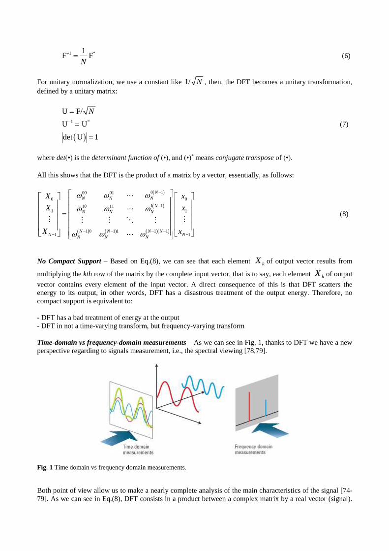
Time-domain vs frequency-domain measurements – As we can see in Fig. 1, thanks to DFT we have a new

perspective regarding to signals measurement, i.e., the spectral viewing [78,79].

Fig. 1 Time domain vs frequency domain measurements.

Both point of view allow us to make a nearly complete analysis of the main characteristics of the signal [74-

79]. As we can see in Eq.(8), DFT consists in a product between a complex matrix by a real vector (signal).

This gives us a vector output also complex [78, 79]. Therefore, for practical reasons, it is more useful to use

the Power Spectral Density (PSD) [74-79].

For example, in MATLAB®, we have

f = 10;

overSampRate = 30;

fs = overSampRate*f;

phase = 1/3*pi;

nCyl = 5;

t = 0:1/fs:nCyl*1/f;

x = sin(2*pi*f*t+phase);

L = length(x);

NFFT = 1024;

X = fftshift(fft(x,NFFT));

PSD = X.*conj(X)/(NFFT*L);

fVals = fs*(0:NFFT/2-1)/NFFT;

% frequency of sine wave

% oversampling rate

% sampling frequency

% desired phase shift in radians

% to generate five cycles of sine wave

% time base

% replace with cos if a cosine wave is desired

% length of sine wave

% number of considered FFT points

% application of DFT (for practical reasons FFT, see next subsection)

% Power of each frequency components

% deleting negative frequencies

If we rewrite Eq.(8), we will have

FX x (In MATLAB® code, X = fftshift(fft(x,NFFT));) (9)

where X is the output vector (frequency domain), F is the DFT matrix (see Eq.3), and x is the input vector

(time domain), then

PSD

X . conj X

NFFT L

(In MATLAB® code, PSD = X .* conj(X)/(NFFT*L);) (10)

In Eq.(10), “ .” means infixed version of Hadamard’s product of vectors [80], e.g., if we have two vectors

0 1NA a ,...,a and 0 1NB b ,...,b , then 0 0 1 1 1 1N NA. B a b , a b ,..., a b , while conj(•) means

complex conjugate of (•), while, “” means simply product of scalars.

In DSP, some authors work with the square root of PSD [74-77], and others - on the contrary - with the

modulus (or absolute value) of X [78, 79], directly.

Spectral analysis - When the DFT is used for signal spectral analysis, the nx sequence usually represents

a finite set of uniformly spaced time-samples of some signal x(t), where t represents time. The conversion

from continuous time to samples (discrete-time) changes the underlying Fourier transform of x(t) into a

discrete-time Fourier transform (DTFT), which generally entails a type of distortion called aliasing. Choice

of an appropriate sample-rate (see Nyquist rate) is the key to minimizing that distortion. Similarly, the

conversion from a very long (or infinite) sequence to a manageable size entails a type of distortion called

leakage, which is manifested as a loss of detail (a.k.a. resolution) in the DTFT. Choice of an appropriate sub-

sequence length is the primary key to minimizing that effect. When the available data (and time to process it)

is more than the amount needed to attain the desired frequency resolution, a standard technique is to perform

multiple DFTs, for example to create a spectrogram. If the desired result is a power spectrum and noise or

randomness is present in the data, averaging the magnitude components of the multiple DFTs is a useful

procedure to reduce the variance of the spectrum (also called a periodogram in this context); two examples of

such techniques are the Welch method and the Bartlett method; the general subject of estimating the power

spectrum of a noisy signal is called spectral estimation.

A final source of distortion (or perhaps illusion) is the DFT itself, because it is just a discrete sampling of the

DTFT, which is a function of a continuous frequency domain. That can be mitigated by increasing the

resolution of the DFT. That procedure is illustrated at sampling the DTFT [78, 79].

- The procedure is sometimes referred to as zero-padding, which is a particular implementation used in

conjunction with the fast Fourier transform (FFT) algorithm. The inefficiency of performing multiplica-

tions and additions with zero-valued samples is more than offset by the inherent efficiency of the FFT.

- As already noted, leakage imposes a limit on the inherent resolution of the DTFT. So there is a practical

limit to the benefit that can be obtained from a fine-grained DFT.

Summing-up, we summarize the most important advantages and disadvantages of DFT.

Disadvantages:

- DFT fails at the edges. This is the reason why in the JPEG algorithm (employed in image compression)

we use the DCT instead of DFT [45-48]. Even, discrete Hartley transform has an outperform to DFT in

DSP and DIP [45, 46].

- No compact support, therefore, to arrive at the frequency domain the correspondence element by element

between the two domains (time and frequency) is lost, with a lousy treatment of energy.

- As a consequence of not having compact support, it is not at time. In fact, it moves away from the time

domain. For this reason, in the last decades, the scientific community has created some palliatives with

better performance in both domain simultaneously, i.e., time and frequency, such tools are: STFT, GT,

and wavelets.

- DFT has phase uncertainties (indeterminate phase for magnitude = 0) [78,79].

- As it arises from the product of a matrix by a vector, its computational cost is O(N2) for signals (1D), and

O(N4) for images (2D).

All this would seem to indicate that it is a bad transform, however, they are its advantages that keep it afloat.

Then, we describe here only some of them.

Advantages:

- As the decisions (relative to filtering and compression) are taken in the spectral domain, the DFT is in its

element for both applications. Although as we mentioned before, given its problem with the edges, we use

DCT instead DFT.

- It makes the convolutions easier when we use the fast release of DFT, i.e., FFT.

- It is separable (separability property), which is extremely useful when DFT should apply to bi and three-

dimensional arrays [45-48].

- Given its internal canonical form (distribution of twiddle factors within the DFT matrix), it allows faster

versions of itself, such as FFT.

2.1.3 FFT

Fast Fourier Transform - FFT inherits all the disadvantages of the DFT, except the computational

complexity of this. In fact, and unlike DFT, the computational cost of FFT is O(N*log2N) for signals (1D),

and O((N*log2N)2) for images (2D). For this, it is called fast Fourier transform.

FFT is an algorithm that computes the Discrete Fourier Transform (DFT) of a sequence, or its inverse.

Fourier analysis converts a signal from its original domain (often time or space) to the frequency domain and

vice versa. An FFT rapidly computes such transformations by factorizing the DFT matrix into a product of

sparse (mostly zero) factors [81, 82]. As a result, it manages to reduce the complexity of computing the DFT

from O(N2), which arises if one simply applies the definition of DFT, to O(N*log2N), where N is the data

size. The computational cost for this technique is never greater than the conventional approach and usually

significantly less. Further, the computational cost as a function of n is highly continuous, so that linear

convolutions of sizes somewhat larger than a power of two.

FFT are widely used for many applications in engineering, science, and mathematics. The basic ideas were

popularized in 1965, but some algorithms had been derived as early as 1805 [83]. In 1994 Gilbert Strang

described the fast Fourier transform as the most important numerical algorithm of our lifetime [84] and it

was included in Top 10 Algorithms of 20th Century by the IEEE journal Computing in Science &

Engineering [85].

Overview - There are many different FFT algorithms involving a wide range of mathematics, from simple

complex-number arithmetic to group theory and number theory; this article gives an overview of the

available techniques and some of their general properties, while the specific algorithms are described in

subsidiary articles linked below.

The DFT is obtained by decomposing a sequence of values into components of different frequencies. This

operation is useful in many fields (see discrete Fourier transform for properties and applications of the

transform) but computing it directly from the definition is often too slow to be practical. An FFT is a way to

compute the same result more quickly: computing the DFT of N points in the naive way, using the definition,

takes O(N2) arithmetical operations, while an FFT can compute the same DFT in only O(N*log2N)

operations. The difference in speed can be enormous, especially for long data sets where N may be in the

thousands or millions. In practice, the computation time can be reduced by several orders of magnitude in

such cases, and the improvement is roughly proportional to N/log2N. This huge improvement made the

calculation of the DFT practical; FFTs are of great importance to a wide variety of applications, from digital

signal processing and solving partial differential equations to algorithms for quick multiplication of large

integers.

The best-known FFT algorithms depend upon the factorization of N, but there are FFTs with O(N*log2N)

complexity for all N, even for prime N. Many FFT algorithms only depend on the fact that 2 i / Ne

is an N-th

primitive root of unity, and thus can be applied to analogous transforms over any finite field, such as

number-theoretic transforms. Since the inverse DFT is the same as the DFT, but with the opposite sign in the

exponent and a 1/N factor, any FFT algorithm can easily be adapted for it.

History - The development of fast algorithms for DFT can be traced to Gauss's unpublished work in 1805

when he needed it to interpolate the orbit of asteroids Pallas and Juno from sample observations [86]. His

method was very similar to the one published in 1965 by Cooley and Tukey, who are generally credited for

the invention of the modern generic FFT algorithm. While Gauss's work predated even Fourier's results in

1822, he did not analyze the computation time and eventually used other methods to achieve his goal.

Between 1805 and 1965, some versions of FFT were published by other authors. Yates in 1932 published his

version called interaction algorithm, which provided efficient computation of Hadamard and Walsh

transforms [87]. Yates' algorithm is still used in the field of statistical design and analysis of experiments. In

1942, Danielson and Lanczos published their version to compute DFT for x-ray crystallography, a field

where calculation of Fourier transforms presented a formidable bottleneck [88]. While many methods in the

past had focused on reducing the constant factor for O(N2) computation by taking advantage of symmetries,

Danielson and Lanczos realized that one could use the periodicity and apply a "doubling trick" to get

O(N*log2N) runtime [89].

Cooley and Tukey published a more general version of FFT in 1965 that is applicable when N is composite

and not necessarily a power of 2 [90]. Tukey came up with the idea during a meeting of President Kennedy’s

Science Advisory Committee where a discussion topic involved detecting nuclear tests by the Soviet Union

by setting up sensors to surround the country from outside. To analyze the output of these sensors, a fast

Fourier transform algorithm would be needed. Tukey's idea was taken by Richard Garwin and given to

Cooley (both worked at IBM's Watson labs) for implementation while hiding the original purpose from him

for security reasons. The pair published the paper in a relatively short six months [91]. As Tukey didn't work

at IBM, the patentability of the idea was doubted and the algorithm went into the public domain, which,

through the computing revolution of the next decade, made FFT one of the indispensable algorithms in

digital signal processing.

Fourier Uncertainty Principle - In quantum mechanics, the uncertainty principle [92], also known as

Heisenberg's uncertainty principle, is any of a variety of mathematical inequalities asserting a fundamental

limit to the precision with which certain pairs of physical properties of a particle, known as complementary

variables, such as energy E and time t, can be known simultaneously, although p and x are other important,

i.e., position and momentum, respectively. They cannot be simultaneously measured with arbitrarily high

precision. There is a minimum for the product of the uncertainties of these two measurements.

Introduced first in 1927, by the German physicist Werner Heisenberg, it states that the more precisely the

position of some particle is determined, the less precisely its momentum can be known, and vice versa. The

formal inequality relating the uncertainty of energy E and the uncertainty of time t was derived by Earle

Hesse Kennard later that year and by Hermann Weyl in 1928:

/2E t (11)

where ħ is the reduced Planck constant, h / 2π. The energy associated to such system is

E (where = 2f, being f the frequency, and the angular frequency) (12)

Then, any uncertainty about is transferred to the energy, that is to say,

E (13)

Replacing Eq.(13) into (11), we will have,

/2t (14)

Finally, simplifying Eq.(14), we will have,

1/2t (15)

Eq.(15) say us that a simultaneous decimation in time and frequency is impossible for FFT. Therefore, we

must make do with decimate in time or frequency, but not both at once. The four following transforms

(STFT, GT, FrFT, and WT) represent a futile effort -to date- to link more closely (individually) each sample

in time with its counterpart in frequency in a biunivocal correspondence. That is to say, they are transforms

without compact support.

2.1.4 STFT

The short-time Fourier transform (STFT), or alternatively short-term Fourier transform, is a Fourier-

related transform used to determine the sinusoidal frequency and phase content of local sections of a signal

as it changes over time [93, 94]. In practice, the procedure for computing STFTs is to divide a longer time

signal into shorter segments of equal length and then compute the Fourier transform separately on each

shorter segment. This reveals the Fourier spectrum on each shorter segment. One then usually plots the

changing spectra as a function of time.

Continuous-time STFT - Simply, in the continuous-time case, the function to be transformed is multiplied

by a window function which is nonzero for only a short period of time. The Fourier transform (a one-

dimensional function) of the resulting signal is taken as the window is slid along the time axis, resulting in a

two-dimensional representation of the signal. Mathematically, this is written as:

STFT j tx t , X , x t w t e dt

(16)

where w(t) is the window function, commonly a Hann window or Gaussian window bell centered around

zero, and x(t) is the signal to be transformed. (Note the difference between w and ω.) X(τ,ω) is essentially the

Fourier Transform of x(t)w(t-τ), a complex function representing the phase and magnitude of the signal over

time and frequency. Often phase unwrapping is employed along either or both the time axis, τ, and frequency

axis, ω, to suppress any jump discontinuity of the phase result of the STFT. The time index τ is normally

considered to be "slow" time and usually not expressed in as high resolution as time t. The STFT represents

an effort to try to fix the spectral components almost instantaneously, i.e., linked wings temporary signal

samples.

Discrete-time STFT - In the discrete time case, the data to be transformed could be broken up into chunks or

frames (which usually overlap each other, to reduce artifacts at the boundary). Each chunk is Fourier

transformed, and the complex result is added to a matrix, which records magnitude and phase for each point

in time and frequency. This can be expressed as:

STFT j n

n

x n m, X m, x n w n m e

(17)

likewise, with signal x[n] and window w[n]. In this case, m is discrete and ω is continuous, but in most

typical applications the STFT is performed on a computer using the Fast Fourier Transform, so both

variables are discrete and quantized.

The magnitude squared of the STFT yields the spectrogram of the function:

2

spectrogram x t , X , (18)

See also the modified discrete cosine transform (MDCT), which is also a Fourier-related transform that uses

overlapping windows.

Sliding DFT - If only a small number of ω are desired, or if the STFT is desired to be evaluated for every

shift m of the window, then the STFT may be more efficiently evaluated using a sliding DFT algorithm [95].

Inverse STFT - The STFT is invertible, that is, the original signal can be recovered from the transform by

the Inverse STFT. The most widely accepted way of inverting the STFT is by using the overlap-add (OLA)

method, which also allows for modifications to the STFT complex spectrum. This makes for a versatile

signal processing method [96], referred to as the overlap and add with modifications method.

Continuous-time STFT - Given the width and definition of the window function w(t), we initially require the

area of the window function to be scaled so that

1w d .

(19)

It easily follows that

1w t d t

(20)

and

x t x t w t d x t w t d .

(21)

The continuous Fourier Transform is

j tX x t e dt.

(22)

Substituting x(t) from above:

j t

j t

X x t w t d e dt

x t w t e d dt.

(23)

Swapping order of integration:

j t

j t

X x t w t e dt d

x t w t e dt d

X , d .

(24)

So the Fourier Transform can be seen as a sort of phase coherent sum of all of the STFTs of x(t). Since the

inverse Fourier transform is

1

2π

j tx t X e d ,

(25)

then x(t) can be recovered from X(τ,ω) as

1

2π

j tx t X , e d d ,

(26)

or

1

2π

j tx t X , e d d .

(27)

It can be seen, comparing to above that windowed "grain" or "wavelet" of x(t) is

1

2π

j tx t w t X , e d .

(28)

the inverse Fourier transform of X(τ,ω) for τ fixed.

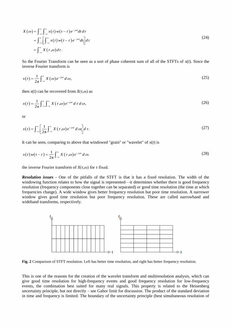
Resolution issues - One of the pitfalls of the STFT is that it has a fixed resolution. The width of the

windowing function relates to how the signal is represented—it determines whether there is good frequency

resolution (frequency components close together can be separated) or good time resolution (the time at which

frequencies change). A wide window gives better frequency resolution but poor time resolution. A narrower

window gives good time resolution but poor frequency resolution. These are called narrowband and

wideband transforms, respectively.

Fig. 2 Comparison of STFT resolution. Left has better time resolution, and right has better frequency resolution.

This is one of the reasons for the creation of the wavelet transform and multiresolution analysis, which can

give good time resolution for high-frequency events and good frequency resolution for low-frequency

events, the combination best suited for many real signals. This property is related to the Heisenberg

uncertainty principle, but not directly – see Gabor limit for discussion. The product of the standard deviation

in time and frequency is limited. The boundary of the uncertainty principle (best simultaneous resolution of

both) is reached with a Gaussian window function, as the Gaussian minimizes the Fourier uncertainty

principle. This is called the Gabor transform (and with modifications for multiresolution becomes the Morlet

wavelet transform). One can consider the STFT for varying window size as a two-dimensional domain (time

and frequency), as illustrated in the example below, which can be calculated by varying the window size.

However, this is no longer a strictly time–frequency representation – the kernel is not constant over the entire

signal.

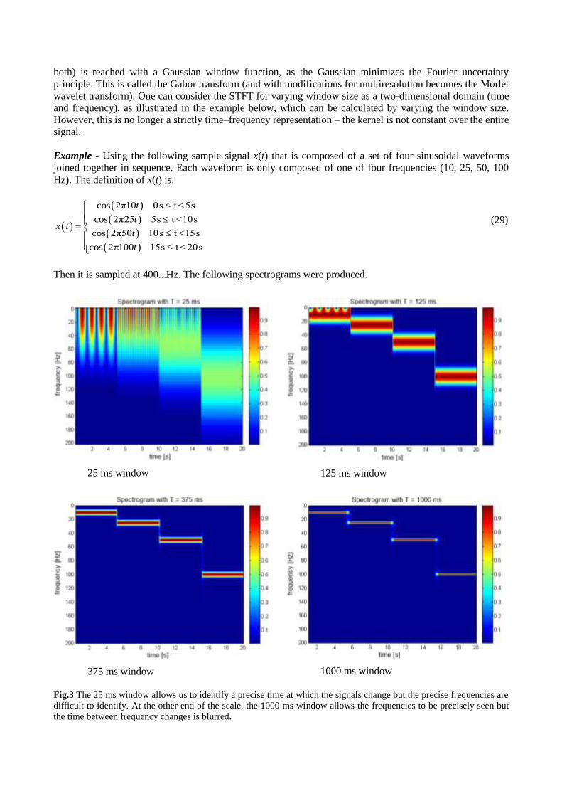
Example - Using the following sample signal x(t) that is composed of a set of four sinusoidal waveforms

joined together in sequence. Each waveform is only composed of one of four frequencies (10, 25, 50, 100

Hz). The definition of x(t) is:

cos 2π10 0s t <5s

cos 2π25 5s t <10s

cos 2π50 10s t <15s

cos 2π100 15s t < 20s

t

tx t

t

t

(29)

Then it is sampled at 400...Hz. The following spectrograms were produced.

25 ms window

125 ms window

375 ms window

1000 ms window

Fig.3 The 25 ms window allows us to identify a precise time at which the signals change but the precise frequencies are

difficult to identify. At the other end of the scale, the 1000 ms window allows the frequencies to be precisely seen but

the time between frequency changes is blurred.

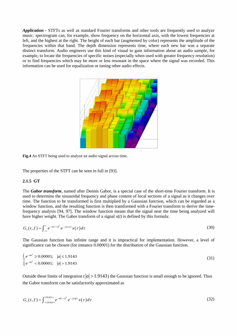
Application - STFTs as well as standard Fourier transforms and other tools are frequently used to analyze

music. spectrogram can, for example, show frequency on the horizontal axis, with the lowest frequencies at

left, and the highest at the right. The height of each bar (augmented by color) represents the amplitude of the

frequencies within that band. The depth dimension represents time, where each new bar was a separate

distinct transform. Audio engineers use this kind of visual to gain information about an audio sample, for

example, to locate the frequencies of specific noises (especially when used with greater frequency resolution)

or to find frequencies which may be more or less resonant in the space where the signal was recorded. This

information can be used for equalization or tuning other audio effects.

Fig.4 An STFT being used to analyze an audio signal across time.

The properties of the STFT can be seen in full in [93].

2.1.5 GT

The Gabor transform, named after Dennis Gabor, is a special case of the short-time Fourier transform. It is

used to determine the sinusoidal frequency and phase content of local sections of a signal as it changes over

time. The function to be transformed is first multiplied by a Gaussian function, which can be regarded as a

window function, and the resulting function is then transformed with a Fourier transform to derive the time-

frequency analysis [94, 97]. The window function means that the signal near the time being analyzed will

have higher weight. The Gabor transform of a signal x(t) is defined by this formula:

2

2t j f

xG t, f e e x d

(30)

The Gaussian function has infinite range and it is impractical for implementation. However, a level of

significance can be chosen (for instance 0.00001) for the distribution of the Gaussian function.

2

2

π

π

0 00001 1 9143

0 00001 1 9143

a

a

e . ; a .

e . ; a .

(31)

Outside these limits of integration ( 1 9143a . ) the Gaussian function is small enough to be ignored. Thus

the Gabor transform can be satisfactorily approximated as

21 9143

π 2π

1 9143

. tt j f

x. t

G t, f e e x d

(32)

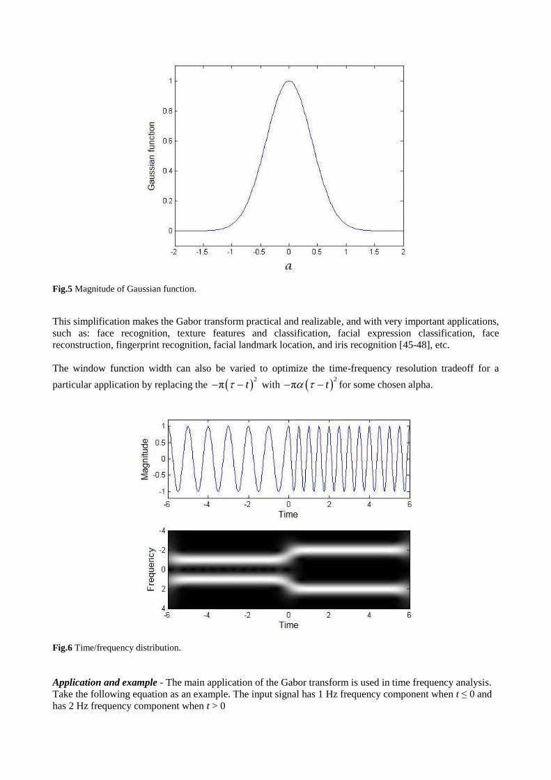
Fig.5 Magnitude of Gaussian function.

This simplification makes the Gabor transform practical and realizable, and with very important applications,

such as: face recognition, texture features and classification, facial expression classification, face

reconstruction, fingerprint recognition, facial landmark location, and iris recognition [45-48], etc.

The window function width can also be varied to optimize the time-frequency resolution tradeoff for a

particular application by replacing the 2

π t with 2

π t for some chosen alpha.

Fig.6 Time/frequency distribution.

Application and example - The main application of the Gabor transform is used in time frequency analysis.

Take the following equation as an example. The input signal has 1 Hz frequency component when t ≤ 0 and

has 2 Hz frequency component when t > 0

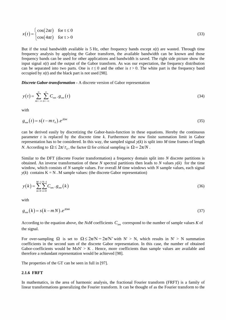
cos 2π for t 0

cos 4π for t 0

tx t

t

(33)

But if the total bandwidth available is 5 Hz, other frequency bands except x(t) are wasted. Through time

frequency analysis by applying the Gabor transform, the available bandwidth can be known and those

frequency bands can be used for other applications and bandwidth is saved. The right side picture show the

input signal x(t) and the output of the Gabor transform. As was our expectation, the frequency distribution

can be separated into two parts. One is t ≤ 0 and the other is t > 0. The white part is the frequency band

occupied by x(t) and the black part is not used [98].

Discrete Gabor-transformation - A discrete version of Gabor representation

nm nm

m n

y t C .g t

(34)

with

Ω

0

j nt

nmg t s t m .e (35)

can be derived easily by discretizing the Gabor-basis-function in these equations. Hereby the continuous

parameter t is replaced by the discrete time k. Furthermore the now finite summation limit in Gabor

representation has to be considered. In this way, the sampled signal y(k) is split into M time frames of length

N. According to 0Ω 2π/ , the factor Ω for critical sampling is Ω 2π/N .

Similar to the DFT (discrete Fourier transformation) a frequency domain split into N discrete partitions is

obtained. An inverse transformation of these N spectral partitions then leads to N values y(k) for the time

window, which consists of N sample values. For overall M time windows with N sample values, each signal

y(k) contains K = N M sample values: (the discrete Gabor representation)

1 1

0 0

M N

nm nm

m n

y k C .g k

(36)

with

Ωj nk

nmg k s k m N .e (37)

According to the equation above, the NxM coefficients nmC correspond to the number of sample values K of

the signal.

For over-sampling Ω is set to Ω 2π/N = 2π/N' with N' > N, which results in N' > N summation

coefficients in the second sum of the discrete Gabor representation. In this case, the number of obtained

Gabor-coefficients would be MxN' > K . Hence, more coefficients than sample values are available and

therefore a redundant representation would be achieved [98].

The properties of the GT can be seen in full in [97].

2.1.6 FRFT

In mathematics, in the area of harmonic analysis, the fractional Fourier transform (FRFT) is a family of

linear transformations generalizing the Fourier transform. It can be thought of as the Fourier transform to the

n-th power, where n need not be an integer — thus, it can transform a function to any intermediate domain

between time and frequency. Its applications range from filter design and signal analysis to phase retrieval

and pattern recognition.

The FRFT can be used to define fractional convolution, correlation, and other operations, and can also be

further generalized into the linear canonical transformation (LCT). An early definition of the FRFT was

introduced by Condon [99, 100], by solving for the Green's function for phase-space rotations, and also by

Namias [101], generalizing work of Wiener [102] on Hermite polynomials. However, it was not widely

recognized in signal processing until it was independently reintroduced around 1993 by several groups [103].

Since then, there has been a surge of interest in extending Shannon's sampling theorem [104, 105] for signals

which are band-limited in the Fractional Fourier domain.

A completely different meaning for "fractional Fourier transform" was introduced –after that– by Bailey and

Swartztrauber [106] as essentially another name for a z-transform, and in particular for the case that

corresponds to a discrete Fourier transform shifted by a fractional amount in frequency space (multiplying

the input by a linear chirp) and evaluating at a fractional set of frequency points (e.g. considering only a

small portion of the spectrum). Such transforms can be evaluated efficiently by Bluestein's FFT algorithm.

This terminology has fallen out of use in most of the technical literature, however, in preference to the FRFT.

Introduction - As we can see in Subsection 2.1.1, the Fourier transform (or, continuous Fourier transform)

of a function ƒ: is a unitary operator of L2 that maps the function ƒ to its frequential version f :

2 ixf f x e dx

, for any real number ξ. (38)

And ƒ is determined by f via the inverse transform 1

2 ixf x f e d

, for any real number x. (39)

Let us study its n-th iterated n

defined by 1n nf f and 1n

n when n is a non-

negative integer, and 0 f f . Their sequence is finite since is a 4-periodic automorphism: for every

function ƒ, 4 f f .

More precisely, let us introduce the parity operator that inverts time, f : t f t . Then the

following properties hold:

0 1 2 4

3 1

Id Id, , , ,

.

(40)

The FrFT provides a family of linear transforms that further extends this definition to handle non-integer

powers n = 2α/π of the FT.

Definition - For any real α, the α-angle fractional Fourier transform of a function ƒ is denoted by u and

defined by

2

2

cot α2π csc α

2πcot α1 cot α dx.

i ux xi u

f u i e e f x

(41)

(the square root is defined such that the argument of result lies in the interval π/2 π/2, )

If α is an integer multiple of π, then the cotangent and cosecant functions above diverge. However, this can

be handled by taking the limit, and leads to a Dirac delta function in the integrand. More directly, since

2 f f t , f must be simply f(t) or f(−t) for α an even or odd multiple of π, respectively.

For α = π/2, this becomes precisely the definition of the continuous Fourier transform, and for α = −π/2 it is

the definition of the inverse continuous Fourier transform.

The FrFT argument u is neither a spatial one x nor a frequency ξ. We will see why it can be interpreted as

linear combination of both coordinates (x, ξ). When we want to distinguish the α-angular fractional domain,

we will let xa denote the argument of α .

Remark: with the angular frequency ω convention instead of the frequency one, the FrFT formula is the

Mehler kernel,

2 2cot α /2 csc α cot α /21 cot αd .

2π

i i t tif e e f t t

(42)

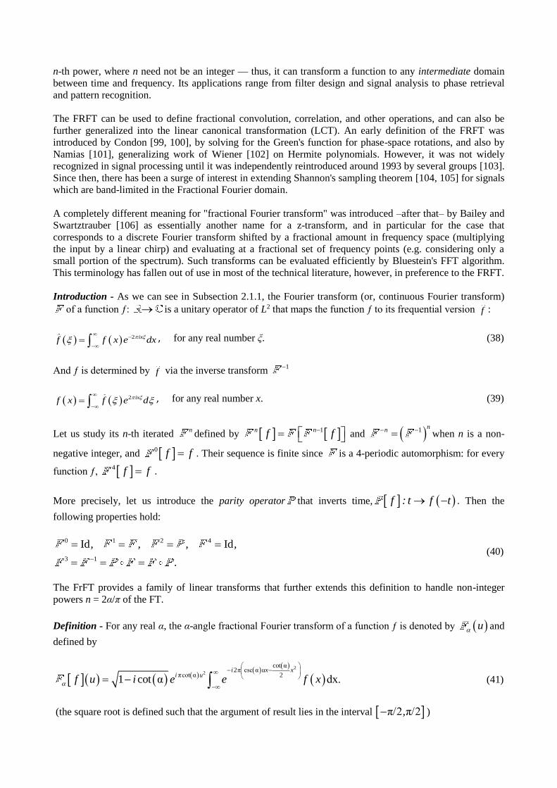
Interpretation of the fractional Fourier transform - The usual interpretation of the Fourier transform is as a

transformation of a time domain signal into a frequency domain signal. On the other hand, the interpretation

of the inverse Fourier transform is as a transformation of a frequency domain signal into a time domain

signal. Apparently, fractional Fourier transforms can transform a signal (either in the time domain or

frequency domain) into the domain between time and frequency: it is a rotation in the time-frequency

domain. This perspective is generalized by the linear canonical transformation, which generalizes the

fractional Fourier transform and allows linear transforms of the time-frequency domain other than rotation.

Fig.7 Time/frequency distribution of fractional Fourier transform.

Take the below figure as an example. If the signal in the time domain is rectangular (as below), it will

become a sinc function in the frequency domain. But if we apply the fractional Fourier transform to the

rectangular signal, the transformation output will be in the domain between time and frequency.

Actually, fractional Fourier transform is a rotation operation on the time frequency distribution. From the

definition above, for α = 0, there will be no change after applying fractional Fourier transform, and for

α = π/2, fractional Fourier transform becomes a Fourier transform, which rotates the time frequency

distribution with π/2. For other value of α, fractional Fourier transform rotates the time frequency

distribution according to α. The following figure shows the results of the fractional Fourier transform with

different values of α.

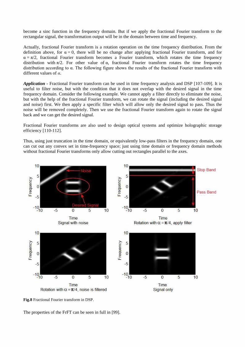
Application - Fractional Fourier transform can be used in time frequency analysis and DSP [107-109]. It is

useful to filter noise, but with the condition that it does not overlap with the desired signal in the time

frequency domain. Consider the following example. We cannot apply a filter directly to eliminate the noise,

but with the help of the fractional Fourier transform, we can rotate the signal (including the desired signal

and noise) first. We then apply a specific filter which will allow only the desired signal to pass. Thus the

noise will be removed completely. Then we use the fractional Fourier transform again to rotate the signal

back and we can get the desired signal.

Fractional Fourier transforms are also used to design optical systems and optimize holographic storage

efficiency [110-112].

Thus, using just truncation in the time domain, or equivalently low-pass filters in the frequency domain, one

can cut out any convex set in time-frequency space; just using time domain or frequency domain methods

without fractional Fourier transforms only allow cutting out rectangles parallel to the axes.

Fig.8 Fractional Fourier transform in DSP.

The properties of the FrFT can be seen in full in [99].

2.2 Wavelets in general, and Haar basis in particular

2.2.1 Wavelets in general

In mathematics, a wavelet series is a representation of a square-integrable (real- or complex-valued) function

by a certain orthonormal series generated by a wavelet. Nowadays, wavelet transformation is one of the most

popular candidates of the time-frequency-transformations [113]. This article provides a formal, mathematical

definition of an orthonormal wavelet and of the integral wavelet transform.

Definition - A function 2L is called an orthonormal wavelet if it can be used to define a Hilbert

basis [113-116], that is a complete orthonormal system, for the Hilbert space 2L of square integrable

functions. The Hilbert basis is constructed as the family of functions jk : j,k by means of dyadic

translations and dilations of ,

22 2j

j

jk x x k (43)

for integers j,k .

If under the standard inner product on 2L ,

f ,g f x g x dx

(44)

this family is orthonormal, it is an orthonormal system:

jk lm jk lm

jl km

, x x dx

(45)

where jl is the Kronecker delta.

Completeness is satisfied if every function 2h L may be expanded in the basis as

jk jk

j ,k

h x c x

(46)

with convergence of the series understood to be convergence in norm. Such a representation of a function f is

known as a wavelet series. This implies that an orthonormal wavelet is self-dual [117, 118].

Wavelet transform - The integral wavelet transform [119] is the integral transform defined as

1 x b

W f a,b f x dxaa

(47)

The wavelet coefficients jkc are then given by

2 2j j

jkc W f ,k

(48)

Here, 2 ja is called the binary dilation or dyadic dilation, and 2 jb k is the binary or dyadic position.

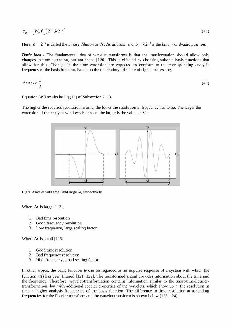
Basic idea - The fundamental idea of wavelet transforms is that the transformation should allow only

changes in time extension, but not shape [120]. This is effected by choosing suitable basis functions that

allow for this. Changes in the time extension are expected to conform to the corresponding analysis

frequency of the basis function. Based on the uncertainty principle of signal processing,

1Δ Δω

2t (49)

Equation (49) results be Eq.(15) of Subsection 2.1.3.

The higher the required resolution in time, the lower the resolution in frequency has to be. The larger the

extension of the analysis windows is chosen, the larger is the value of Δt .

Fig.9 Wavelet with small and larget, respectively.

When Δt is large [113],

1. Bad time resolution

2. Good frequency resolution

3. Low frequency, large scaling factor

When Δt is small [113]

1. Good time resolution

2. Bad frequency resolution

3. High frequency, small scaling factor

In other words, the basis function can be regarded as an impulse response of a system with which the

function x(t) has been filtered [121, 122]. The transformed signal provides information about the time and

the frequency. Therefore, wavelet-transformation contains information similar to the short-time-Fourier-

transformation, but with additional special properties of the wavelets, which show up at the resolution in

time at higher analysis frequencies of the basis function. The difference in time resolution at ascending

frequencies for the Fourier transform and the wavelet transform is shown below [123, 124].

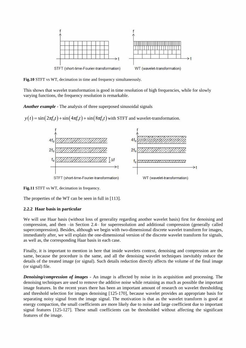
Fig.10 STFT vs WT, decimation in time and frequency simultaneously.

This shows that wavelet transformation is good in time resolution of high frequencies, while for slowly

varying functions, the frequency resolution is remarkable.

Another example - The analysis of three superposed sinusoidal signals

0 0 0sin 2π sin 4π sin 8πy t f t f t f t with STFT and wavelet-transformation.

Fig.11 STFT vs WT, decimation in frequency.

The properties of the WT can be seen in full in [113].

2.2.2 Haar basis in particular

We will use Haar basis (without loss of generality regarding another wavelet basis) first for denoising and

compression, and then –in Section 2.4– for superresolution and additional compression (generally called

supercompression). Besides, although we begin with two-dimensional discrete wavelet transform for images,

immediately after, we will explain the one-dimensional version of the discrete wavelet transform for signals,

as well as, the corresponding Haar basis in each case.

Finally, it is important to mention in here that inside wavelets context, denoising and compression are the

same, because the procedure is the same, and all the denoising wavelet techniques inevitably reduce the

details of the treated image (or signal). Such details reduction directly affects the volume of the final image

(or signal) file.

Denoising/compression of images - An image is affected by noise in its acquisition and processing. The

denoising techniques are used to remove the additive noise while retaining as much as possible the important

image features. In the recent years there has been an important amount of research on wavelet thresholding

and threshold selection for images denoising [125-170], because wavelet provides an appropriate basis for

separating noisy signal from the image signal. The motivation is that as the wavelet transform is good at

energy compaction, the small coefficients are more likely due to noise and large coefficient due to important

signal features [125-127]. These small coefficients can be thresholded without affecting the significant

features of the image.

In fact, the thresholding technique is the last approach based on wavelet theory to provide an enhanced

approach for eliminating such noise source [128, 129] and ensure better image quality [130, 131].

Thresholding is a simple non-linear technique, which operates on one wavelet coefficient at a time. In its

basic form, each coefficient is thresholded by comparing against threshold, if the coefficient is smaller than

threshold, set to zero; otherwise it is kept or modified. Replacing the small noisy coefficients by zero and

inverse wavelet transform on the result may lead to reconstruction with the essential signal characteristics

and with less noise. Since the work of Donoho & Johnstone [125-127], there has been much research on

finding thresholds, however few are specifically designed for images [138-170].

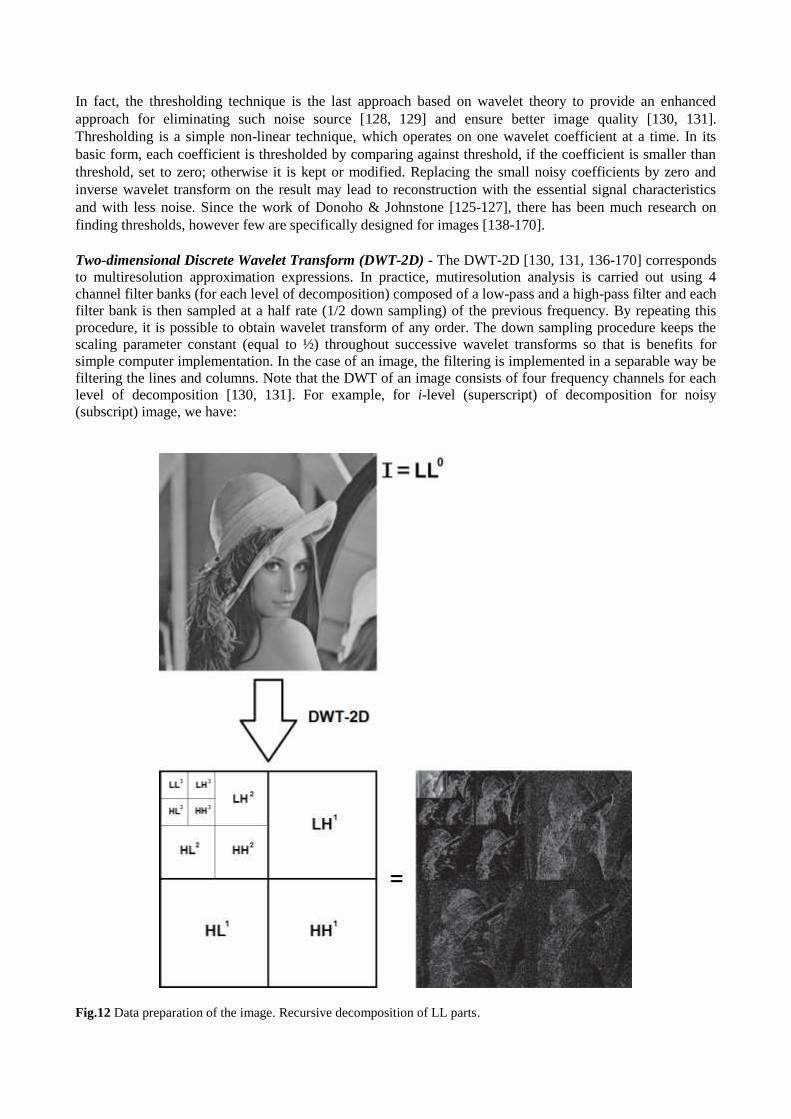
Two-dimensional Discrete Wavelet Transform (DWT-2D) - The DWT-2D [130, 131, 136-170] corresponds

to multiresolution approximation expressions. In practice, mutiresolution analysis is carried out using 4

channel filter banks (for each level of decomposition) composed of a low-pass and a high-pass filter and each

filter bank is then sampled at a half rate (1/2 down sampling) of the previous frequency. By repeating this

procedure, it is possible to obtain wavelet transform of any order. The down sampling procedure keeps the

scaling parameter constant (equal to ½) throughout successive wavelet transforms so that is benefits for

simple computer implementation. In the case of an image, the filtering is implemented in a separable way be

filtering the lines and columns. Note that the DWT of an image consists of four frequency channels for each

level of decomposition [130, 131]. For example, for i-level (superscript) of decomposition for noisy

(subscript) image, we have:

Fig.12 Data preparation of the image. Recursive decomposition of LL parts.

i

nLL : Noisy Coefficients of Approximation.

i

nLH : Noisy Coefficients of Horizontal Detail,

i

nHL : Noisy Coefficients of Vertical Detail, and

i

nHH : Noisy Coefficients of Diagonal Detail.

The LL part at each scale is decomposed recursively, as illustrated in Fig. 12 [130, 131].

Fig.13 Detail of level decomposition for down-right image of Fig.12.

Figure 13 shows –in detail– three levels of decomposition for gray version of Lena. In this figure, we can see

that the splitting occurs from the subband of approximation coefficients, always. Each application of DWT-

2D provides four subbands, which, every LLi will have less noise and size as the previous one, i.e., LLi-1.

To achieve space-scale adaptive noise reduction, we need to prepare the 1-D coefficient data stream which

contains the space-scale information of 2-D images. This is somewhat similar to the “zigzag” arrangement of

the DCT (Discrete Cosine Transform) coefficients in image coding applications [169]. In this data

preparation step, the DWT-2D coefficients are rearranged as a 1-D coefficient series in spatial order so that

the adjacent samples represent the same local areas in the original image [165].

Figure 14 shows inside of DWT-2D with the four subbands of the transformed image [170], while Fig.15

shows inside of IDWT-2D (which is the inverse of DWT-2D), both, i.e., DWT-2D and IDWT-2d will be

used in Fig.16. Each output of Fig. 14 represents a subband of splitting process of the 2-D coefficient matrix

corresponding to Fig. 12. More split levels are not shown to avoid complicating the figures 14 and 15.

Fig.14 DWT-2D. A decomposition step. Usual splitting of the subbands.

Fig.15 Inverse DWT-2D (IDWT-2D). A recomposition step. Usual integration of the subbands.

This stage does not do much except for splitting the image into four disjoint sets of pixels. In our case one

group consists of the low frequency indexed pixels in one subband and the other group consists of three high

frequency subbands of indexed pixels. Each subband contains a quarter as many pixels as the original image.

The splitting into low and high frequency is called the Lazy wavelet transform.

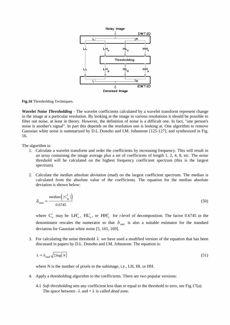
Fig.16 Thresholding Techniques.

Wavelet Noise Thresholding - The wavelet coefficients calculated by a wavelet transform represent change

in the image at a particular resolution. By looking at the image in various resolutions it should be possible to

filter out noise, at least in theory. However, the definition of noise is a difficult one. In fact, "one person's

noise is another's signal". In part this depends on the resolution one is looking at. One algorithm to remove

Gaussian white noise is summarized by D.L. Donoho and I.M. Johnstone [125-127], and synthesized in Fig.

16.

The algorithm is:

1. Calculate a wavelet transform and order the coefficients by increasing frequency. This will result in

an array containing the image average plus a set of coefficients of length 1, 2, 4, 8, etc. The noise

threshold will be calculated on the highest frequency coefficient spectrum (this is the largest

spectrum).

2. Calculate the median absolute deviation (mad) on the largest coefficient spectrum. The median is

calculated from the absolute value of the coefficients. The equation for the median absolute

deviation is shown below:

mad

in

C

0.6745δ

median | | (50)

where i

nC may be i

nLH , i

nHL , or i

nHH for i-level of decomposition. The factor 0.6745 in the

denominator rescales the numerator so that mad is also a suitable estimator for the standard

deviation for Gaussian white noise [5, 165, 169].

3. For calculating the noise threshold λ we have used a modified version of the equation that has been

discussed in papers by D.L. Donoho and I.M. Johnstone. The equation is:

madλ δ 2 Nlog (51)

where N is the number of pixels in the subimage, i.e., LH, HL or HH.

4. Apply a thresholding algorithm to the coefficients. There are two popular versions:

4.1 Soft thresholding sets any coefficient less than or equal to the threshold to zero, see Fig.17(a).

The space between – and + is called dead zone.

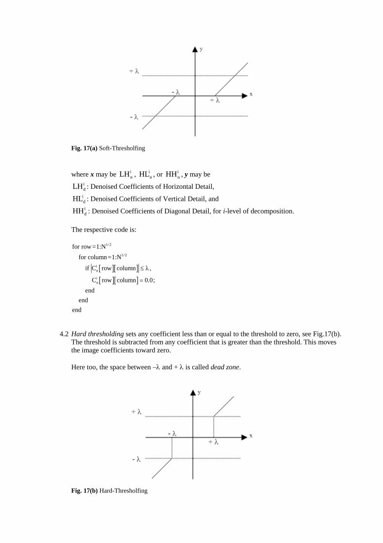
Fig. 17(a) Soft-Thresholfing

where x may be i

nLH , i

nHL , or i

nHH , y may be

i

dLH : Denoised Coefficients of Horizontal Detail,

i

dHL : Denoised Coefficients of Vertical Detail, and

i

dHH : Denoised Coefficients of Diagonal Detail, for i-level of decomposition.

The respective code is:

1 2

1 2

i

n

i

n

for row =1:N

for column =1:N

if C row column λ ,

C row column 0 0;

end

end

end

/

/

.

4.2 Hard thresholding sets any coefficient less than or equal to the threshold to zero, see Fig.17(b).

The threshold is subtracted from any coefficient that is greater than the threshold. This moves

the image coefficients toward zero.

Here too, the space between – and + is called dead zone.

Fig. 17(b) Hard-Thresholfing

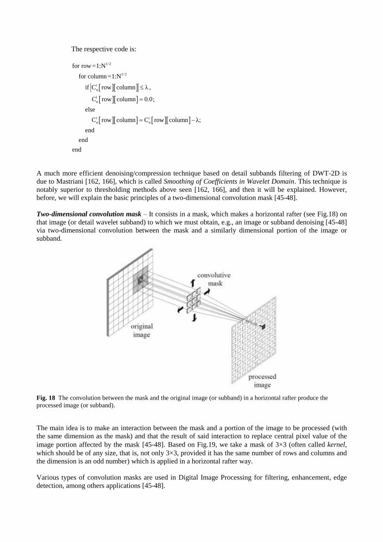
The respective code is:

1 2

1 2

i

n

i

n

i i

n n

for row =1:N

for column =1:N

if C row column λ ,

C row column 0 0;

else

C row column C row column λ;

end

end

end

/

/

.

A much more efficient denoising/compression technique based on detail subbands filtering of DWT-2D is

due to Mastriani [162, 166], which is called Smoothing of Coefficients in Wavelet Domain. This technique is

notably superior to thresholding methods above seen [162, 166], and then it will be explained. However,

before, we will explain the basic principles of a two-dimensional convolution mask [45-48].

Two-dimensional convolution mask – It consists in a mask, which makes a horizontal rafter (see Fig.18) on

that image (or detail wavelet subband) to which we must obtain, e.g., an image or subband denoising [45-48]

via two-dimensional convolution between the mask and a similarly dimensional portion of the image or

subband.

Fig. 18 The convolution between the mask and the original image (or subband) in a horizontal rafter produce the

processed image (or subband).

The main idea is to make an interaction between the mask and a portion of the image to be processed (with

the same dimension as the mask) and that the result of said interaction to replace central pixel value of the

image portion affected by the mask [45-48]. Based on Fig.19, we take a mask of 3×3 (often called kernel,

which should be of any size, that is, not only 3×3, provided it has the same number of rows and columns and

the dimension is an odd number) which is applied in a horizontal rafter way.

Various types of convolution masks are used in Digital Image Processing for filtering, enhancement, edge

detection, among others applications [45-48].

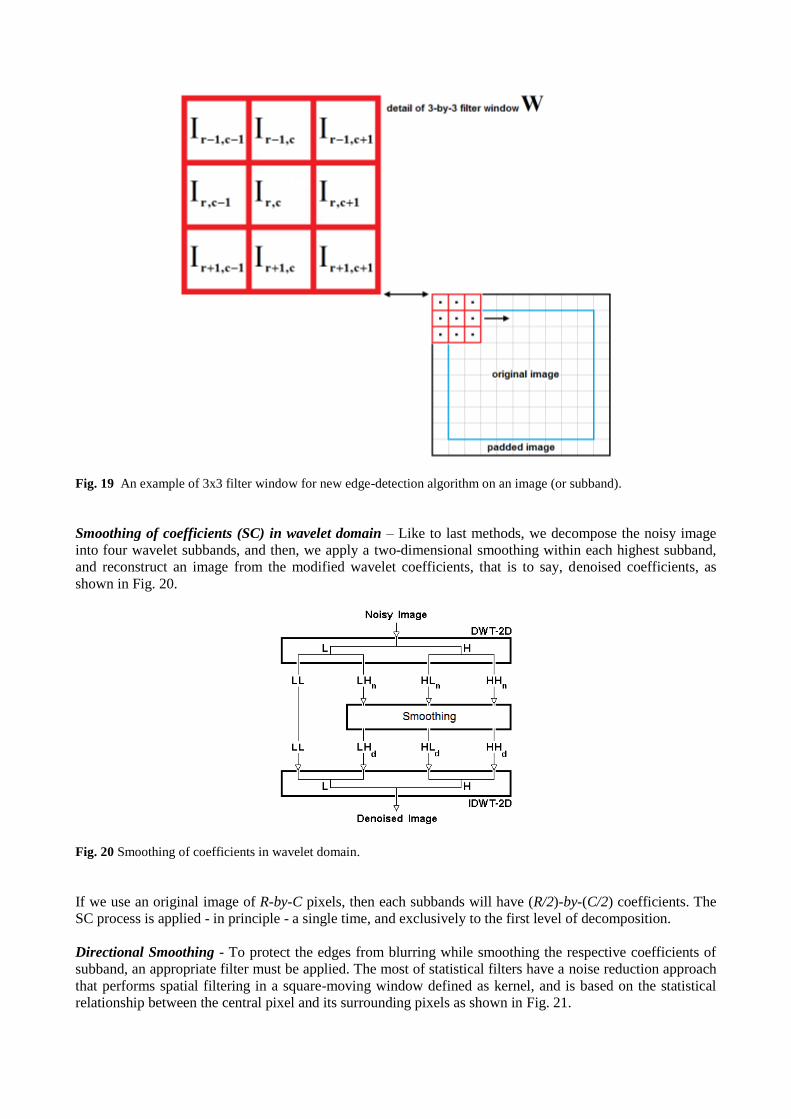
Fig. 19 An example of 3x3 filter window for new edge-detection algorithm on an image (or subband).

Smoothing of coefficients (SC) in wavelet domain – Like to last methods, we decompose the noisy image

into four wavelet subbands, and then, we apply a two-dimensional smoothing within each highest subband,

and reconstruct an image from the modified wavelet coefficients, that is to say, denoised coefficients, as

shown in Fig. 20.

Fig. 20 Smoothing of coefficients in wavelet domain.

If we use an original image of R-by-C pixels, then each subbands will have (R/2)-by-(C/2) coefficients. The

SC process is applied - in principle - a single time, and exclusively to the first level of decomposition.

Directional Smoothing - To protect the edges from blurring while smoothing the respective coefficients of

subband, an appropriate filter must be applied. The most of statistical filters have a noise reduction approach

that performs spatial filtering in a square-moving window defined as kernel, and is based on the statistical

relationship between the central pixel and its surrounding pixels as shown in Fig. 21.

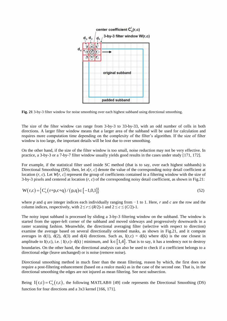
Fig. 21 3-by-3 filter window for noise smoothing over each highest subband using directional smoothing.

The size of the filter window can range from 3-by-3 to 33-by-33, with an odd number of cells in both

directions. A larger filter window means that a larger area of the subband will be used for calculation and

requires more computation time depending on the complexity of the filter’s algorithm. If the size of filter

window is too large, the important details will be lost due to over smoothing.

On the other hand, if the size of the filter window is too small, noise reduction may not be very effective. In

practice, a 3-by-3 or a 7-by-7 filter window usually yields good results in the cases under study [171, 172].

For example, if the statistical filter used inside SC method (that is to say, over each highest subbands) is

Directional Smoothing (DS), then, let x[r, c] denote the value of the corresponding noisy detail coefficient at

location (r, c). Let W[r, c] represent the group of coefficients contained in a filtering window with the size of

3-by-3 pixels and centered at location (r, c) of the corresponding noisy detail coefficient, as shown in Fig.21:

i

nW r,c C r+p,c+q p,q 1 0 1/ , , (52)

where p and q are integer indices each individually ranging from −1 to 1. Here, r and c are the row and the

column indices, respectively, with 2 ≤ r ≤ (R/2)-1 and 2 ≤ c ≤ (C/2)-1.

The noisy input subband is processed by sliding a 3-by-3 filtering window on the subband. The window is

started from the upper-left corner of the subband and moved sideways and progressively downwards in a

raster scanning fashion. Meanwhile, the directional averaging filter (selective with respect to direction)

examine the average based on several directionally oriented masks, as shown in Fig.21, and it compute

averages in d(1), d(2), d(3) and d(4) directions. Such as, I(r,c) = d(k) where d(k) is the one closest in

amplitude to I(r,c), i.e. | I(r,c)- d(k) | minimum, and k 1 4, . That is to say, it has a tendency not to destroy

boundaries. On the other hand, the directional analysis can also be used to check if a coefficient belongs to a

directional edge (leave unchanged) or is noise (remove noise).

Directional smoothing method in much finer than the mean filtering, reason by which, the first does not

require a post-filtering enhancement (based on a realce mask) as in the case of the second one. That is, in the

directional smoothing the edges are not injured as mean filtering. See next subsection.

Being i

nI r,c C r,c , the following MATLAB® [49] code represents the Directional Smoothing (DS)

function for four directions and a 3x3 kernel [166, 171].

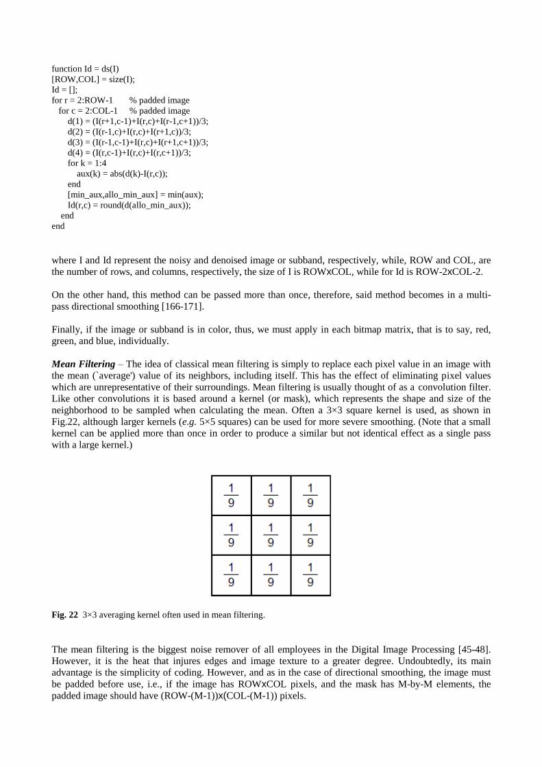
function Id = ds(I)

[ROW,COL] = size(I);

Id = [];

for r = 2:ROW-1 % padded image

for c = 2:COL-1 % padded image

d(1) = (I(r+1,c-1)+I(r,c)+I(r-1,c+1))/3;

d(2) = (I(r-1,c)+I(r,c)+I(r+1,c))/3;

d(3) = (I(r-1,c-1)+I(r,c)+I(r+1,c+1))/3;

d(4) = (I(r,c-1)+I(r,c)+I(r,c+1))/3;

for k = 1:4

aux(k) = abs(d(k)-I(r,c));

end

[min_aux,allo_min_aux] = min(aux);

Id(r,c) = round(d(allo_min_aux));

end

end

where I and Id represent the noisy and denoised image or subband, respectively, while, ROW and COL, are

the number of rows, and columns, respectively, the size of I is ROWxCOL, while for Id is ROW-2xCOL-2.

On the other hand, this method can be passed more than once, therefore, said method becomes in a multi-

pass directional smoothing [166-171].

Finally, if the image or subband is in color, thus, we must apply in each bitmap matrix, that is to say, red,

green, and blue, individually.

Mean Filtering – The idea of classical mean filtering is simply to replace each pixel value in an image with

the mean (`average') value of its neighbors, including itself. This has the effect of eliminating pixel values

which are unrepresentative of their surroundings. Mean filtering is usually thought of as a convolution filter.

Like other convolutions it is based around a kernel (or mask), which represents the shape and size of the

neighborhood to be sampled when calculating the mean. Often a 3×3 square kernel is used, as shown in

Fig.22, although larger kernels (e.g. 5×5 squares) can be used for more severe smoothing. (Note that a small

kernel can be applied more than once in order to produce a similar but not identical effect as a single pass

with a large kernel.)

Fig. 22 3×3 averaging kernel often used in mean filtering.

The mean filtering is the biggest noise remover of all employees in the Digital Image Processing [45-48].

However, it is the heat that injures edges and image texture to a greater degree. Undoubtedly, its main

advantage is the simplicity of coding. However, and as in the case of directional smoothing, the image must

be padded before use, i.e., if the image has ROWxCOL pixels, and the mask has M-by-M elements, the

padded image should have (ROW-(M-1))x(COL-(M-1)) pixels.

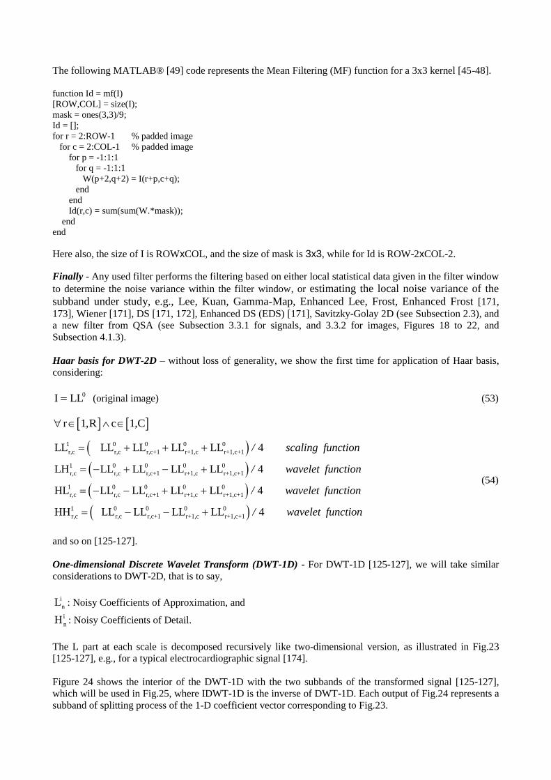
The following MATLAB® [49] code represents the Mean Filtering (MF) function for a 3x3 kernel [45-48].

function Id = mf(I)

[ROW,COL] = size(I);

mask = ones(3,3)/9;

Id = [];

for r = 2:ROW-1 % padded image

for c = 2:COL-1 % padded image

for p = -1:1:1

for q = -1:1:1

W(p+2,q+2) = I(r+p,c+q);

end

end

Id(r,c) = sum(sum(W.*mask));

end

end

Here also, the size of I is ROWxCOL, and the size of mask is 3x3, while for Id is ROW-2xCOL-2.

Finally - Any used filter performs the filtering based on either local statistical data given in the filter window

to determine the noise variance within the filter window, or estimating the local noise variance of the

subband under study, e.g., Lee, Kuan, Gamma-Map, Enhanced Lee, Frost, Enhanced Frost [171,

173], Wiener [171], DS [171, 172], Enhanced DS (EDS) [171], Savitzky-Golay 2D (see Subsection 2.3), and

a new filter from QSA (see Subsection 3.3.1 for signals, and 3.3.2 for images, Figures 18 to 22, and

Subsection 4.1.3).

Haar basis for DWT-2D – without loss of generality, we show the first time for application of Haar basis,

considering:

0I LL (original image) (53)

r 1 R c 1 C, ,

1 0 0 0 0

r,c r,c r,c+1 r+1,c r+1,c+1

1 0 0 0 0

r,c r,c r,c+1 r+1,c r+1,c+1

1 0 0 0 0

r,c r,c r,c+1 r+1,c r+1,c+1

1 0

r,c r,c r,c+1

LL LL LL LL LL 4

LH LL LL LL LL 4

HL LL LL LL LL 4

HH LL LL

/ scaling function

/ wavelet function

/ wavelet function

0 0 0

r+1,c r+1,c+1LL LL 4/ wavelet function

(54)

and so on [125-127].

One-dimensional Discrete Wavelet Transform (DWT-1D) - For DWT-1D [125-127], we will take similar

considerations to DWT-2D, that is to say,

i

nL : Noisy Coefficients of Approximation, and

i

nH : Noisy Coefficients of Detail.

The L part at each scale is decomposed recursively like two-dimensional version, as illustrated in Fig.23

[125-127], e.g., for a typical electrocardiographic signal [174].

Figure 24 shows the interior of the DWT-1D with the two subbands of the transformed signal [125-127],

which will be used in Fig.25, where IDWT-1D is the inverse of DWT-1D. Each output of Fig.24 represents a

subband of splitting process of the 1-D coefficient vector corresponding to Fig.23.

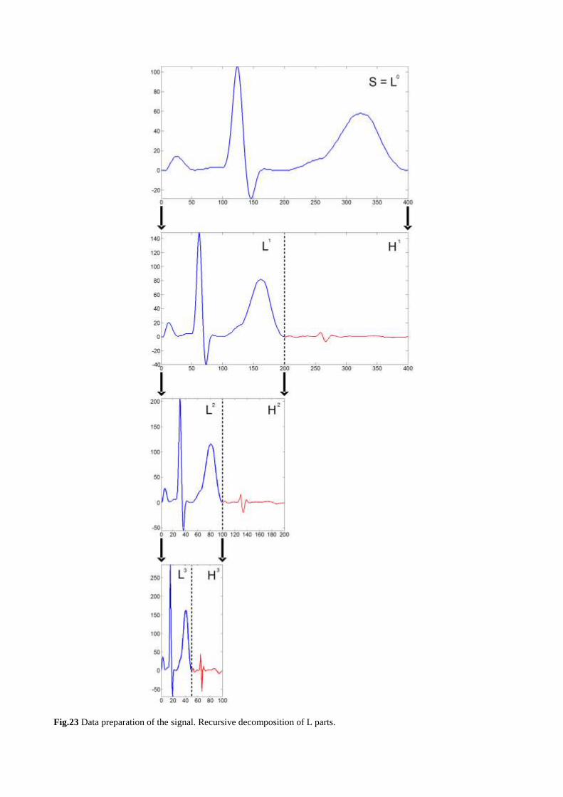
Fig.23 Data preparation of the signal. Recursive decomposition of L parts.

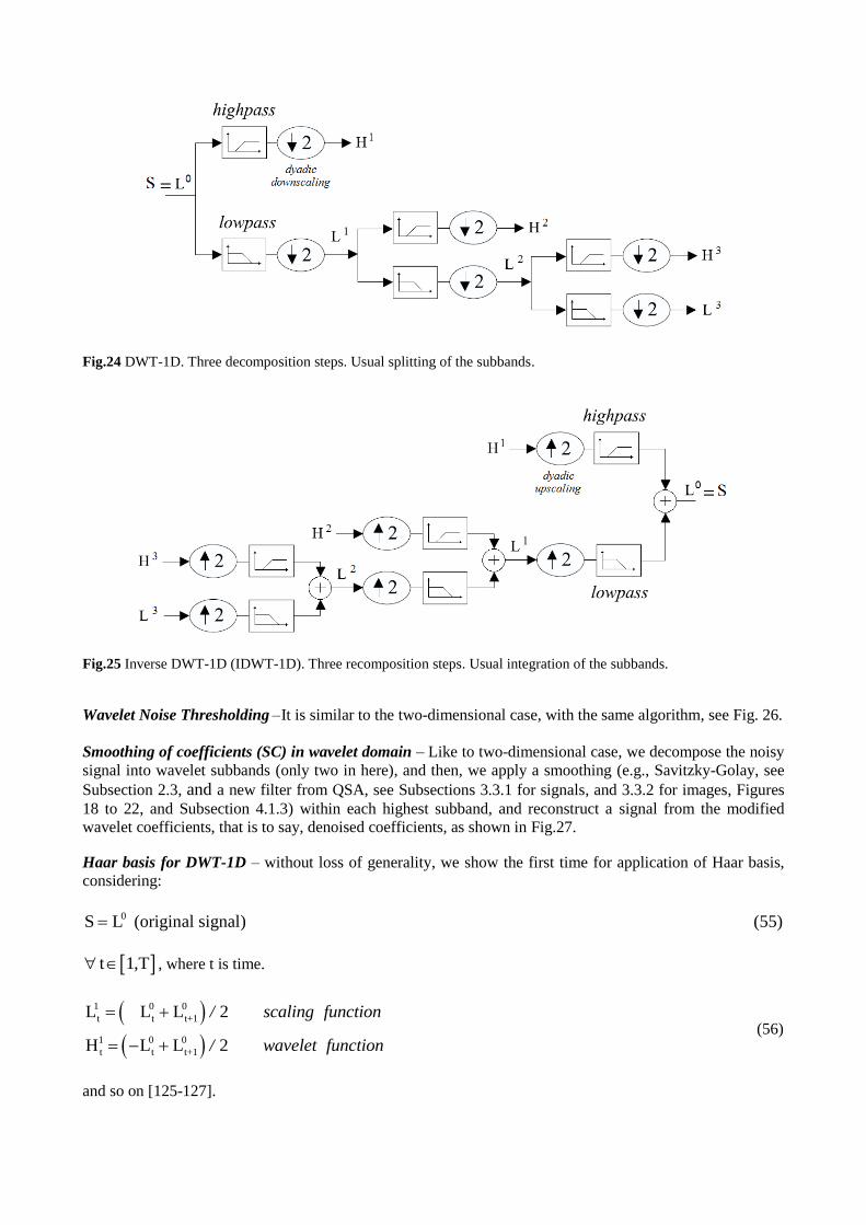
Fig.24 DWT-1D. Three decomposition steps. Usual splitting of the subbands.

Fig.25 Inverse DWT-1D (IDWT-1D). Three recomposition steps. Usual integration of the subbands.

Wavelet Noise Thresholding – It is similar to the two-dimensional case, with the same algorithm, see Fig. 26.

Smoothing of coefficients (SC) in wavelet domain – Like to two-dimensional case, we decompose the noisy

signal into wavelet subbands (only two in here), and then, we apply a smoothing (e.g., Savitzky-Golay, see

Subsection 2.3, and a new filter from QSA, see Subsections 3.3.1 for signals, and 3.3.2 for images, Figures

18 to 22, and Subsection 4.1.3) within each highest subband, and reconstruct a signal from the modified

wavelet coefficients, that is to say, denoised coefficients, as shown in Fig.27.

Haar basis for DWT-1D – without loss of generality, we show the first time for application of Haar basis,

considering:

0S L (original signal) (55)

t 1 T, , where t is time.

1 0 0

t t t+1

1 0 0

t t t+1

L L L 2

H L L 2

/ scaling function

/ wavelet function

(56)

and so on [125-127].

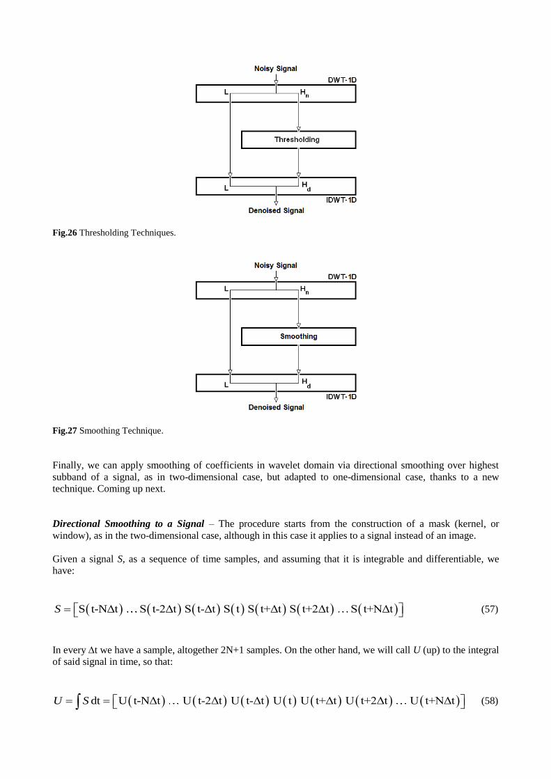
Fig.26 Thresholding Techniques.

Fig.27 Smoothing Technique.

Finally, we can apply smoothing of coefficients in wavelet domain via directional smoothing over highest

subband of a signal, as in two-dimensional case, but adapted to one-dimensional case, thanks to a new

technique. Coming up next.

Directional Smoothing to a Signal – The procedure starts from the construction of a mask (kernel, or

window), as in the two-dimensional case, although in this case it applies to a signal instead of an image.

Given a signal S, as a sequence of time samples, and assuming that it is integrable and differentiable, we

have:

S t-NΔt S t-2Δt S t-Δt S t S t+Δt S t+2Δt S t+NΔtS (57)

In every t we have a sample, altogether 2N+1 samples. On the other hand, we will call U (up) to the integral

of said signal in time, so that:

dt U t-NΔt U t-2Δt U t-Δt U t U t+Δt U t+2Δt U t+NΔtU S (58)

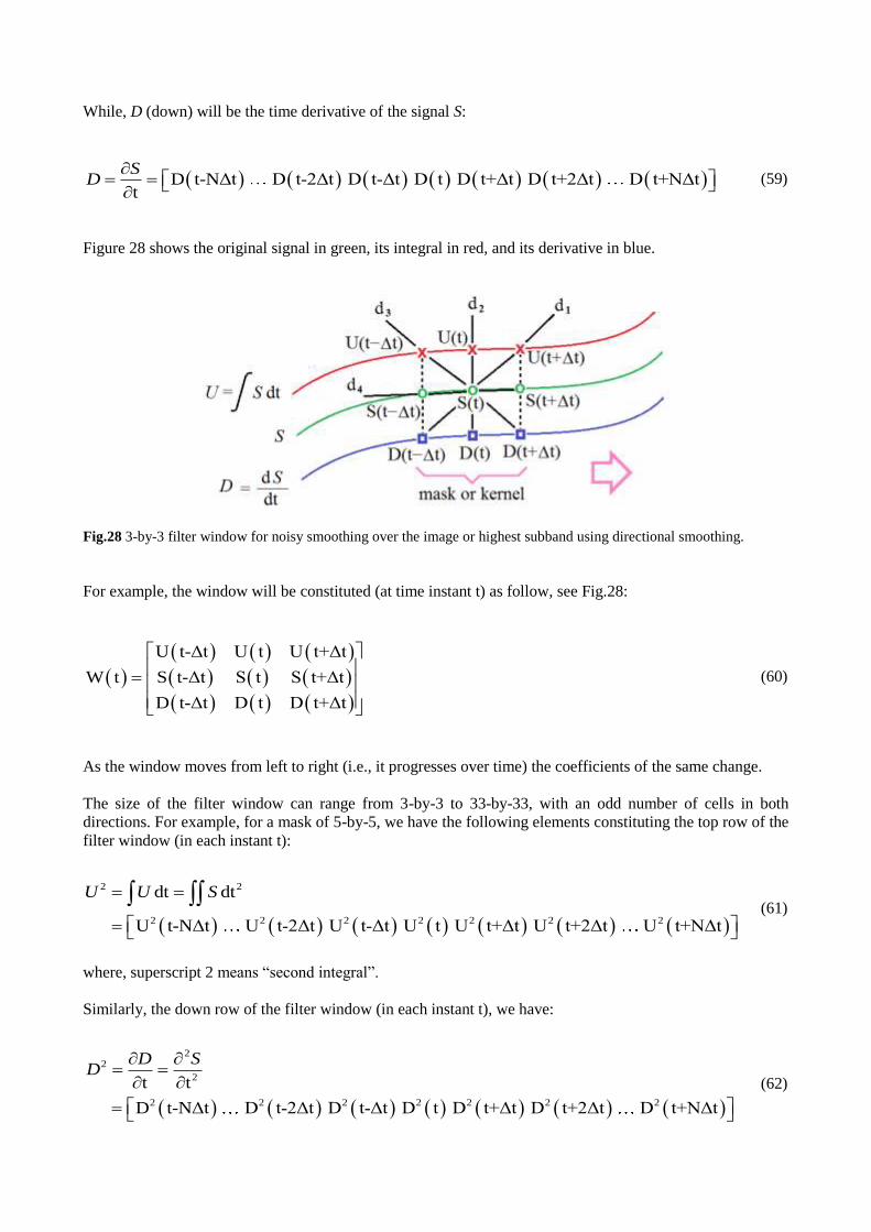
While, D (down) will be the time derivative of the signal S:

D t-NΔt D t-2Δt D t-Δt D t D t+Δt D t+2Δt D t+NΔtt

SD

(59)

Figure 28 shows the original signal in green, its integral in red, and its derivative in blue.

Fig.28 3-by-3 filter window for noisy smoothing over the image or highest subband using directional smoothing.

For example, the window will be constituted (at time instant t) as follow, see Fig.28:

U t-Δt U t U t+Δt

W t S t-Δt S t S t+Δt

D t-Δt D t D t+Δt

(60)

As the window moves from left to right (i.e., it progresses over time) the coefficients of the same change.

The size of the filter window can range from 3-by-3 to 33-by-33, with an odd number of cells in both

directions. For example, for a mask of 5-by-5, we have the following elements constituting the top row of the

filter window (in each instant t):

2 2

2 2 2 2 2 2 2

dt dt

U t-NΔt U t-2Δt U t-Δt U t U t+Δt U t+2Δt U t+NΔt

U U S

(61)

where, superscript 2 means “second integral”.

Similarly, the down row of the filter window (in each instant t), we have:

22

2

2 2 2 2 2 2 2

t t

D t-NΔt D t-2Δt D t-Δt D t D t+Δt D t+2Δt D t+NΔt

D SD

(62)

where, superscript 2 means “second derivative”.

Then, the filter window in this case will be:

2 2 2 2 2

2 2 2 2 2

U t-2Δt U t-Δt U t U t+Δt U t+2Δt

U t-2Δt U t-Δt U t U t+Δt U t+2Δt

S t-2Δt S t-Δt S t S t+Δt S t+2ΔtW t

D t-2Δt D t-Δt D t D t+Δt D t+2Δt

D t-2Δt D t-Δt D t D t+Δt D t+2Δt

(63)

and similarly for larger window.

From this point, the procedure is similar to the two-dimensional case, thus, it only remains to adapt the

corresponding algorithm to the one-dimensional case environment. Therefore, the following MATLAB®

[49] code represents the Directional Smoothing (DS) function for four directions and a 3x3 kernel for signal

denoising.

function Sd = ds(S)

T = length(S);

% Padding signal

% aux_S = [ 0 S 0 ]; % for non-cyclical signals

aux_S = [ S(T) S S(1) ]; % for cyclical signals

D = [];

for n = -N+1:N-1

t = n-(-N+1)+3;

D(t-2) = (aux_S(t)-aux_S(t-2))/2;

end

U = cumsum(S);

Sd = [];

for n = -N+1:N-1

t = n-(-N+1)+2;

d(1) = (D(t-1)+S(t)+U(t+1))/3;

d(2) = (D(t)+S(t)+U(t))/3;

d(3) = (D(t+1)+S(t)+U(t-1))/3;

d(4) = (S(t-1)+S(t)+S(t+1))/3;

for k = 1:4

aux(k) = abs(d(k)-S(t));

end

[min_aux,allo_min_aux] = min(aux);

Sd(t-1) = d(allo_aux_min);

end

end

where T = 2N+1, with –N+1 ≤ t ≤ N-1, Sd is the denoised signal or subband. While, the size of S, U and D is

T, the size of Sd is T-2 = 2N-1 (padded signal or subband).

Note: this tool was created by the author for this paper.

Mean Filtering to a Signal – Similar to two-dimensional case, the idea of classical mean filtering applied to

a signal is simply to replace each sample S(t) of this with the mean (`average') value of its neighbors (in

window), including itself, see Fig. 29.

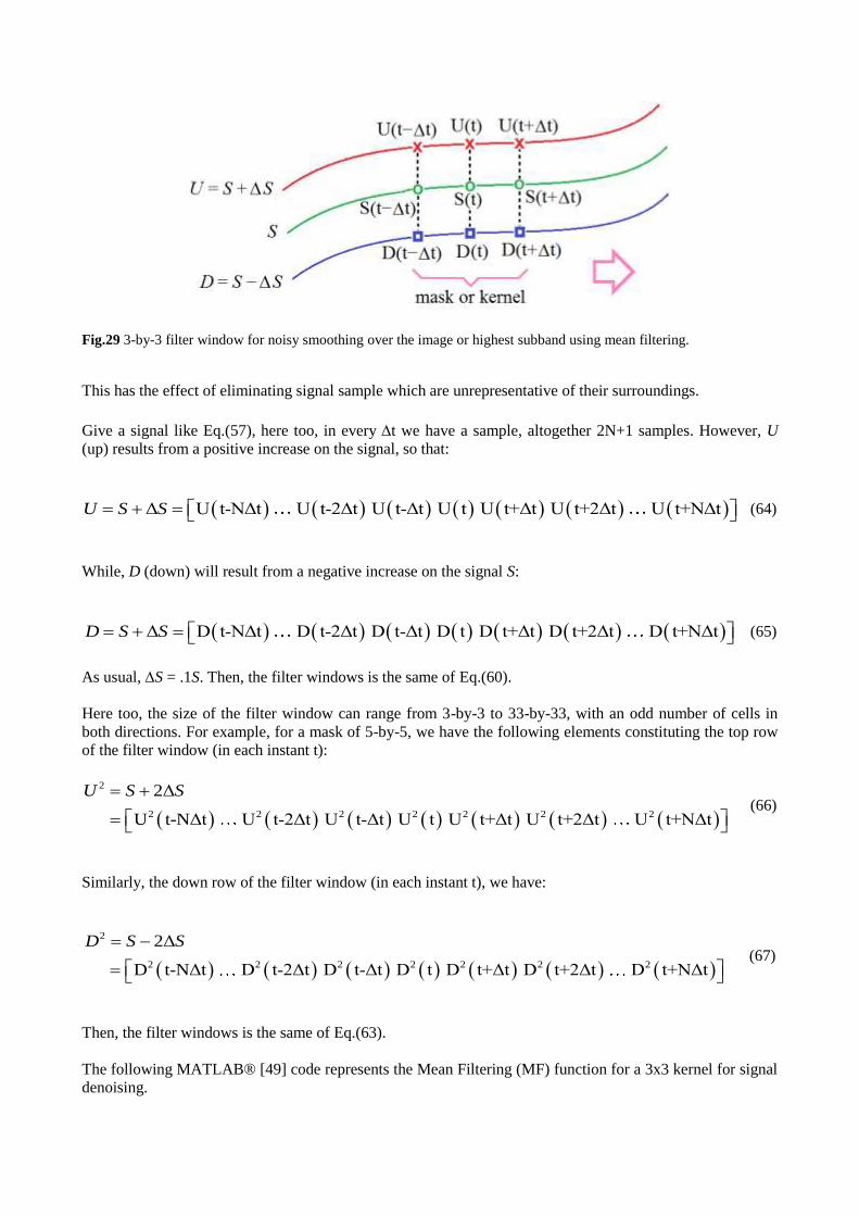
Fig.29 3-by-3 filter window for noisy smoothing over the image or highest subband using mean filtering.

This has the effect of eliminating signal sample which are unrepresentative of their surroundings.

Give a signal like Eq.(57), here too, in every t we have a sample, altogether 2N+1 samples. However, U

(up) results from a positive increase on the signal, so that:

Δ U t-NΔt U t-2Δt U t-Δt U t U t+Δt U t+2Δt U t+NΔtU S S (64)

While, D (down) will result from a negative increase on the signal S:

Δ D t-NΔt D t-2Δt D t-Δt D t D t+Δt D t+2Δt D t+NΔtD S S (65)

As usual, S = .1S. Then, the filter windows is the same of Eq.(60).

Here too, the size of the filter window can range from 3-by-3 to 33-by-33, with an odd number of cells in

both directions. For example, for a mask of 5-by-5, we have the following elements constituting the top row

of the filter window (in each instant t):

2

2 2 2 2 2 2 2

2Δ

U t-NΔt U t-2Δt U t-Δt U t U t+Δt U t+2Δt U t+NΔt

U S S

(66)

Similarly, the down row of the filter window (in each instant t), we have:

2

2 2 2 2 2 2 2

2Δ

D t-NΔt D t-2Δt D t-Δt D t D t+Δt D t+2Δt D t+NΔt

D S S

(67)

Then, the filter windows is the same of Eq.(63).

The following MATLAB® [49] code represents the Mean Filtering (MF) function for a 3x3 kernel for signal

denoising.

function Sd = mf(S)

T = length(S);

U = 1.1*S;

D = 0.9*S;

Sd = [];

for n = -N+1:N-1

t = n-(-N+1)+2;

acuD = 0;

acuS = 0;

acuU = 0;

for aux = -1:1

acuD = acuD + D(t+aux);

acuS = acuS + S(t+aux);

acuU = acuU + U(t+aux);

end

Sd(t-1) = (acuD+acuS+acuU)/9;

end

With similar considerations about Directional Smoothing regarding to names and sizes.

Note: this tool was created by the author for this paper.

2.3 Savitzky-Golay Filtering

A Savitzky–Golay filter (SGF) [175] is a digital filter that can be applied to a set of digital data points for the

purpose of smoothing the data, that is, to increase the signal-to-noise ratio without greatly distorting the

signal. This is achieved, in a process known as convolution, by fitting successive sub-sets of adjacent data

points with a low-degree polynomial by the method of linear least squares. When the data points are equally

spaced an analytical solution to the least-squares equations can be found, in the form of a single set of

"convolution coefficients" that can be applied to all data sub-sets, to give estimates of the smoothed signal,

(or derivatives of the smoothed signal) at the central point of each sub-set. The method, based on established

mathematical procedures [176, 177], was popularized by Abraham Savitzky and Marcel J. E. Golay who

published tables of convolution coefficients for various polynomials and sub-set sizes in 1964 [178, 179].

Some errors in the tables have been corrected [180]. The method has been extended for the treatment of 2-

and 3-dimensional data.

Savitzky and Golay's paper is one of the most widely cited papers in the journal Analytical Chemistry [181]

and is classed by that journal as one of its "10 seminal papers" saying "it can be argued that the dawn of the

computer-controlled analytical instrument can be traced to this article" [182].

SGF [183] is a particular type of low-pass filter, well-adapted for data smoothing, and termed variously

Savitzky-Golay [178], least-squares [184], or DISPO (Digital Smoothing Polynomial) [185] filters. Rather

than having their properties defined in the Fourier domain, and then translated to the time domain, Savitzky-

Golay filters derive directly from a particular formulation of the data smoothing problem in the time domain,

as we will now see. SGFs were initially (and are still often) used to render visible the relative widths and

heights of spectral lines in noisy spectrometric data.

Recall that a digital filter is applied to a series of equally spaced data values fi ≡ f(ti), where ti ≡ t0 + iΔ for

some constant sample spacing Δ and i = . . . − 2,−1, 0, 1, 2, . . . . We have seen [183] that the simplest type

of digital filter (the nonrecursive or finite impulse response filter) replaces each data value fi by a linear

combination gi of itself and some number of nearby neighbors,

R

L

n

i n i n

n n

g c f

(68)

Here nL is the number of points used “to the left” of a data point i, i.e., earlier than it, while nR is the number

used to the right, i.e., later. A so-called causal filter would have nR = 0.

As a starting point for understanding SGFs, consider the simplest possible averaging procedure: For some

fixed nL = nR, compute each gi as the average of the data points from Li nf

to Ri nf

. This is sometimes

called moving window averaging and corresponds to equation (68) with constant cn = 1/(nL +nR +1). If the

underlying function is constant, or is changing linearly with time (increasing or decreasing), then no bias is

introduced into the result. Higher points at one end of the averaging interval are on the average balanced by

lower points at the other end. A bias is introduced, however, if the underlying function has a nonzero second

derivative. At a local maximum, for example, moving window averaging always reduces the function value.

In the spectrometric application, a narrow spectral line has its height reduced and its width increased. Since

these parameters are themselves of physical interest, the bias introduced is distinctly undesirable.

Note, however, that moving window averaging does preserve the area under a spectral line, which is its

zeroth moment, and also (if the window is symmetric with nL = nR) its mean position in time, which is its

first moment. What is violated is the second moment, equivalent to the line width.

The idea of Savitzky-Golay filtering is to find filter coefficients cn that preserve higher moments.

Equivalently, the idea is to approximate the underlying function within the moving window not by a constant

(whose estimate is the average), but by a polynomial of higher order, typically quadratic or quartic: For each

point fi , we least-squares fit a polynomial to all nL + nR +1 points in the moving window, and then set gi to be

the value of that polynomial at position i. We make no use of the value of the polynomial at any other point.

When we move on to the next point fi+1 , we do a whole new least-squares fit using a shifted window.

All these least-squares fits would be laborious if done as described. Luckily, since the process of least-

squares fitting involves only a linear matrix inversion, the coefficients of a fitted polynomial are themselves

linear in the values of the data. That means that we can do all the fitting in advance, for fictitious data

consisting of all zeros except for a single 1, and then do the fits on the real data just by taking linear

combinations. This is the key point, then: There are particular sets of filter coefficients cn for which equation

(68) “automatically” accomplishes the process of polynomial least-squares fitting inside a moving window.

To derive such coefficients, consider how g0 might be obtained: We want to fit a polynomial of degree M in

i, namely a0 + a1i + ・ ・ ・ + aM iM to the values

Lnf , . . . , Rnf . Then g0 will be the value of that

polynomial at i = 0, namely a0 . The design matrix for this problem is

0j

ij L RA i i n , ,n , j , ,M (69)

and the normal equations for the vector of aj ’s in terms of the vector of fi ’s is in matrix notation

1

T T TA A a =Af or a = A A A f

We also have the specific forms

T

ijA A

R R

L L

n ni j

ki kj

k n k n

A A k

(71)

and

T

jA f

R R

L L

n nj

kj k k

k n k n

A f k f

(72)

Since the coefficient cn is the component a0 when f is replaced by the unit vector en , −nL ≤ n < nR , we have

1 1

T T T

0 0 0

A A A e A AM

m

n n

m m

c n

(73)

Note that equation (73) says that we need only one row of the inverse matrix. Numerically we can get this by

LU decomposition with only a single backsubstitution [183].

The accompanying Table I shows some typical Savitzky-Golay coefficients [183]. For orders 2 and 4, the

coefficients of SGFs with several choices of nL and nR are shown. The central column is the coefficient

applied to the data fi in obtaining the smoothed gi. Coefficients to the left are applied to earlier data; to the

right, to later. The coefficients always add (within roundoff error) to unity. One sees that, as befits a

smoothing operator, the coefficients always have a central positive lobe, but with smaller, outlying

corrections of both positive and negative sign. In practice, the SGFs are most useful for much larger values

of nL and nR, since these few-point formulas can accomplish only a relatively small amount of smoothing.

TABLE I

SAMPLE SAVITZKY-GOLAY COEFFICIENTS.

M nL nR Coefficients

2

2

2

2

2

3

4

5

2

1

0

5

-0.086 0.343 0.486 0.343 -0.086

-0.143 0.171 0.343 0.371 0.257

0.086 -0.143 -0.086 0.257 0.886

-0.084 0.021 0.103 0.161 0.196 0.207 0.196 0.161 0.103 0.021 -0.084

4

4

4

5

4

5

0.035 -0.128 0.070 0.315 0.417 0.315 0.070 -0.128 0.035

0.042 -0.105 -0.023 0.140 0.280 0.333 0.280 0.140 -0.023 -0.105 0.042

Fig.30 Top: Synthetic noisy data consisting of a sequence of progressively narrower bumps, and additive Gaussian

white noise. Center: Result of smoothing the data by a simple moving window average. The window extends 16 points

leftward and rightward, for a total of 33 points. Note that narrow features are broadened and suffer corresponding loss

of amplitude. The dotted curve is the underlying function used to generate the synthetic data. Bottom: Result of

smoothing the data by a Savitzky-Golay smoothing filter (of degree 4) using the same 33 points. While there is less

smoothing of the broadest feature, narrower features have their heights and widths preserved.

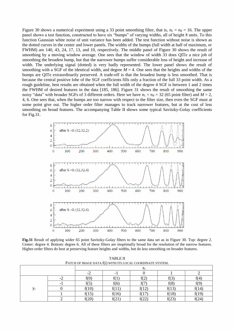
Figure 30 shows a numerical experiment using a 33 point smoothing filter, that is, nL = nR = 16. The upper

panel shows a test function, constructed to have six “bumps” of varying widths, all of height 8 units. To this

function Gaussian white noise of unit variance has been added. The test function without noise is shown as

the dotted curves in the center and lower panels. The widths of the bumps (full width at half of maximum, or

FWHM) are 140, 43, 24, 17, 13, and 10, respectively. The middle panel of Figure 30 shows the result of

smoothing by a moving window average. One sees that the window of width 33 does QITe a nice job of

smoothing the broadest bump, but that the narrower bumps suffer considerable loss of height and increase of

width. The underlying signal (dotted) is very badly represented. The lower panel shows the result of

smoothing with a SGF of the identical width, and degree M = 4. One sees that the heights and widths of the

bumps are QITe extraordinarily preserved. A trade-off is that the broadest bump is less smoothed. That is

because the central positive lobe of the SGF coefficients fills only a fraction of the full 33 point width. As a

rough guideline, best results are obtained when the full width of the degree 4 SGF is between 1 and 2 times

the FWHM of desired features in the data [185, 186]. Figure 31 shows the result of smoothing the same

noisy “data” with broader SGFs of 3 different orders. Here we have nL = nR = 32 (65 point filter) and M = 2,

4, 6. One sees that, when the bumps are too narrow with respect to the filter size, then even the SGF must at

some point give out. The higher order filter manages to track narrower features, but at the cost of less

smoothing on broad features. The accompanying Table II shows some typical Savitzky-Golay coefficients

for Fig.31.

Fig.31 Result of applying wider 65 point Savitzky-Golay filters to the same data set as in Figure 30. Top: degree 2.

Center: degree 4. Bottom: degree 6. All of these filters are inoptimally broad for the resolution of the narrow features.

Higher-order filters do best at preserving feature heights and widths, but do less smoothing on broader features.

TABLE II

PATCH OF IMAGE DATA f(i) WITH ITS LOCAL COORDINATE SYSTEM.

xi

-2 -1 0 1 2

yi

-2 f(0) f(1) f(2) f(3) f(4)

-1 f(5) f(6) f(7) f(8) f(9)

0 f(10) f(11) f(12) f(13) f(14)

1 f(15) f(16) f(17) f(18) f(19)

2 f(20) f(21) f(22) f(23) f(24)

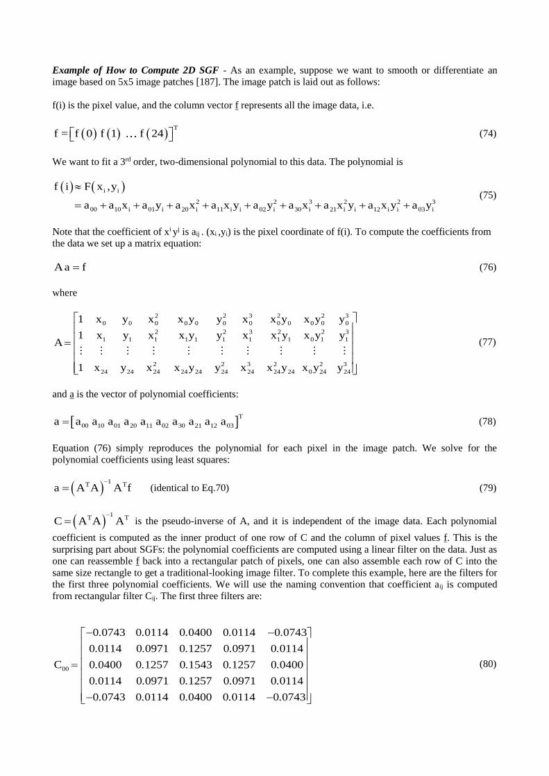
Example of How to Compute 2D SGF - As an example, suppose we want to smooth or differentiate an

image based on 5x5 image patches [187]. The image patch is laid out as follows:

f(i) is the pixel value, and the column vector f represents all the image data, i.e.

T

f = f 0 f 1 f 24 (74)

We want to fit a 3rd order, two-dimensional polynomial to this data. The polynomial is

i i

2 2 3 2 2 3

00 10 i 01 i 20 i 11 i i 02 i 30 i 21 i i 12 i i 03 i

f i F x y

a a x a y a x a x y a y a x a x y a x y a y

,

(75)

Note that the coefficient of xi yj is aij . (xi ,yi) is the pixel coordinate of f(i). To compute the coefficients from

the data we set up a matrix equation:

Aa f (76)

where

22 2 3 2 3

0 00 0 0 0 0 0 0 0 0 0

22 2 3 2 3

0 11 1 1 1 1 1 1 1 1 1

22 2 3 2 3

0 2424 24 24 24 24 24 24 24 24 24

x y1 x y x x y y x x y y

x y1 x y x x y y x x y yA

x y1 x y x x y y x x y y

(77)

and a is the vector of polynomial coefficients:

T

00 10 01 20 11 02 30 21 12 03a a a a a a a a a a a (78)

Equation (76) simply reproduces the polynomial for each pixel in the image patch. We solve for the

polynomial coefficients using least squares:

1

T Ta A A A f

(identical to Eq.70) (79)

1

T TC A A A

is the pseudo-inverse of A, and it is independent of the image data. Each polynomial

coefficient is computed as the inner product of one row of C and the column of pixel values f. This is the

surprising part about SGFs: the polynomial coefficients are computed using a linear filter on the data. Just as

one can reassemble f back into a rectangular patch of pixels, one can also assemble each row of C into the

same size rectangle to get a traditional-looking image filter. To complete this example, here are the filters for

the first three polynomial coefficients. We will use the naming convention that coefficient aij is computed

from rectangular filter Cij. The first three filters are:

00

0 0743 0 0114 0 0400 0 0114 0 0743

0 0114 0 0971 0 1257 0 0971 0 0114

C 0 0400 0 1257 0 1543 0 1257 0 0400

0 0114 0 0971 0 1257 0 0971 0 0114

0 0743 0 0114 0 0400 0 0114 0 0743

. . . . .

. . . . .

. . . . .

. . . . .

. . . . .

(80)

10

0 0738 0 0119 0 0405 0 0119 0 0738

0 1048 0 1476 0 1619 0 1476 0 1048

C 0 0 0 0 0

0 1048 0 1476 0 1619 0 1476 0 1048

0 0738 0 0119 0 0405 0 0119 0 0738

. . . . .

. . . . .

. . . . .

. . . . .

(81)

01

0 0738 0 1048 0 0 1048 0 0738

0 0119 0 1476 0 0 1476 0 0119

C 0 0405 0 1619 0 0 1619 0 0405

0 0119 0 1476 0 0 1476 0 0119

0 0738 0 1048 0 0 1048 0 0738

. . . .

. . . .

. . . .

. . . .

. . . .

(82)

Example of How to Use 2D SGF - Suppose we want to smooth an image. Using a SGFs, we are

conceptually fitting a two-dimensional polynomial to the image patch surrounding each pixel and then

evaluating this polynomial [187]. The local coordinate system that we use for the image patch (see Table II)

has (x,y) = (0,0) at the pixel of interest in the middle of the patch. Thus to compute the smoothed value of the

pixel, we just evaluate the polynomial at (x,y) = (0,0). This turns out to be merely a00, which we can compute

by applying filter C00 to the image patch.

Suppose we want to compute partial derivatives on the patch. The two partial derivatives of the fitted

polynomial are

2 2

x i i 10 20 i 11 i 30 i 21 i i 12 i

2 2

y i i 01 11 i 02 i 21 i 12 i i 03 i

F x , y = a 2a x a y 3a x 2a x y a y

F x , y = a a x 2a y +a x 2a x y 3a y

(83)

Evaluating at (x,y) = (0,0), the results are simply Fx(0,0) = a10 and Fy(0,0) = a01, which are computed with

filters C10 and C01 above.

2.4 Superresolution in general, and for still images in particular

Introduction - Digital image capture produces discrete representations of continuous scenes [188]. This

discretisation in both space and intensity is a sampling process that creates aliasing, and information at

frequencies above the Nyquist rate is lost. It is common to wish to construct a higher resolution image from a

template image or a set of images, but the aliasing and loss of frequency information makes this an ill-posed

(inverse) problem.

The typical solution to this problem (known in the literature as image super-resolution reconstruction, or

simply superresolution) is to use an ensemble of related lower-resolution images. As each of these images

has aliased the higher frequency information slightly differently, under certain conditions it is possible to

“unwrap” some of the aliasing and reconstruct the lost higher frequencies.

There are numerous methods [189-193] of performing super-resolution. Many of them are computationally

expensive in nature, but allow for complicated motion models, significant noise and image degradation, and

other aspects that are not considered in this work. Given assumptions of global translational motion, low

noise and linear space and time invariant blur due to the imaging sensor point spread function (PSF), image

superresolution reconstruction can be split into there distinct steps:

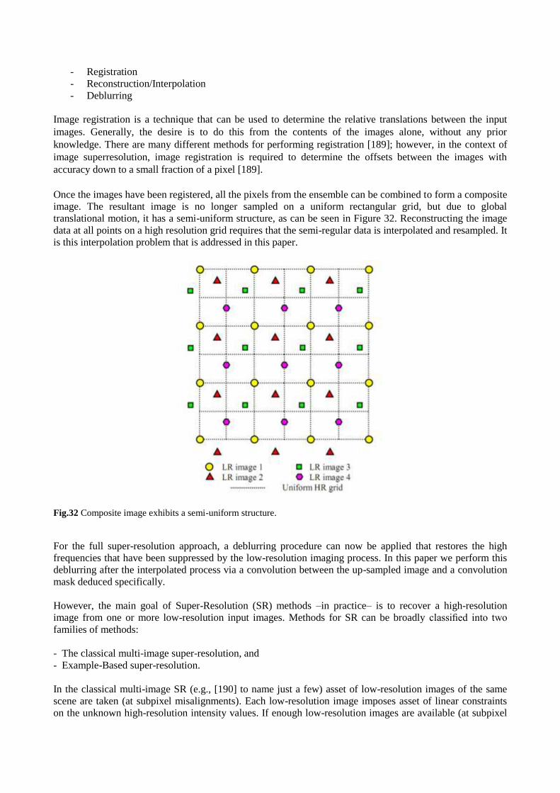
- Registration

- Reconstruction/Interpolation

- Deblurring

Image registration is a technique that can be used to determine the relative translations between the input

images. Generally, the desire is to do this from the contents of the images alone, without any prior

knowledge. There are many different methods for performing registration [189]; however, in the context of

image superresolution, image registration is required to determine the offsets between the images with

accuracy down to a small fraction of a pixel [189].

Once the images have been registered, all the pixels from the ensemble can be combined to form a composite

image. The resultant image is no longer sampled on a uniform rectangular grid, but due to global

translational motion, it has a semi-uniform structure, as can be seen in Figure 32. Reconstructing the image

data at all points on a high resolution grid requires that the semi-regular data is interpolated and resampled. It

is this interpolation problem that is addressed in this paper.

Fig.32 Composite image exhibits a semi-uniform structure.

For the full super-resolution approach, a deblurring procedure can now be applied that restores the high

frequencies that have been suppressed by the low-resolution imaging process. In this paper we perform this

deblurring after the interpolated process via a convolution between the up-sampled image and a convolution

mask deduced specifically.

However, the main goal of Super-Resolution (SR) methods –in practice– is to recover a high-resolution

image from one or more low-resolution input images. Methods for SR can be broadly classified into two

families of methods:

- The classical multi-image super-resolution, and

- Example-Based super-resolution.

In the classical multi-image SR (e.g., [190] to name just a few) asset of low-resolution images of the same

scene are taken (at subpixel misalignments). Each low-resolution image imposes asset of linear constraints

on the unknown high-resolution intensity values. If enough low-resolution images are available (at subpixel

shifts), then the set of equations becomes determined and can be solved to recover the high-resolution image.

Practically, however, this approach is numerically limited only to small increases in resolution [190] (by

factors smaller than 2).

These limitations have lead to the development of “Example-Based Super-Resolution” also termed “image

hallucination” (see references in [190]). In example-based SR, correspondences between low and high-

resolution image patches are learned from a data base of low and high-resolution image pairs (usually with a

relative scale factor of 2), and then applied to a new low-resolution image to recover its most likely high-

resolution version. Higher SR factors have often been obtained by repeated applications of this process.

Example-based SR has been shown to exceed the limits of classical SR. However, unlike classical SR, the

high resolution details reconstructed (“hallucinated”) by example-based SR are not guaranteed to provide the

true (unknown) high-resolution details.

Sophisticated methods for image up-scaling based on learning edge models have also been proposed (e.g.,

[191-193]). The goal of these methods is to magnify (up-scale) an image while maintaining the sharpness of

the edges and the details in the image. In contrast, in SR (example-based as well as classical) the goal is to

recover new missing high-resolution details that are not explicitly found in any individual low-resolution

image (details beyond the Nyquist frequency of the low-resolution image). In the classical SR, this high-

frequency information is assumed to be split across multiple low-resolution images, implicitly found there in

aliased form. In example-based SR, this missing high-resolution information is assumed to be available in

the high-resolution data base patches, and learned from the low-res/high-res pairs of examples in the

database. However beyond what we have said above, in this paper, we consider the interpolation of a single

image.

On the other hand, the rendering of lower resolution image data on higher resolution displays has become a

very common task, in particular because of the increasing popularity of webcams, camera phones, and low-

bandwidth video streaming. Thus, there is a strong demand for real-time, high-quality image magnification.

In this work, we suggest to exploit the high performance of general-purpose computation on programmable

graphics processing units (GPGPUs) for an original image magnification method. To this end, we propose a

GPGPU-friendly algorithm for image up-sampling with edge restoration image interpolation, which avoids

ringing artifacts, excessive blurring, and stair-casing of oblique edges. At the same time it features gray-scale

invariance, is applicable to color images, and allows for real-time processing of full-screen images on

today’s GPGPUs [194-197].

Two-dimensional Interpolation - A digital image is not an exact snapshot of reality, it is only a discrete

approximation. This fact should be apparent to the average web surfer, as images commonly become blocky

or jagged after being resized to fit the browser. The goal of image interpolation is to produce acceptable

images at different resolutions from a single low-resolution image. The actual resolution of an image is

defined as the number of pixels, but the effective resolution is a much harder quantity to define as it depends

on subjective human judgment and perception. The goal of this section is to explore different mathematical

formulations of this essentially aesthetic quantity.

The image interpolation problem goes by many names, depending on the application: image resizing, image

up-sampling/down-sampling, digital zooming, image magnification, resolution enhancement, etc. The term

super-resolution is sometimes used, although in the literature this generally refers to producing a high-

resolution image from multiple images such as a video sequence. If we define interpolation as “filling in the

pixels in between,” the image interpolation problem can be viewed as a subset of the inpainting problem (see

Figure 33).

The applications of image interpolation range from the common place viewing of online images to the more

sophisticated magnification of satellite images. With the rise of consumer-based digital photography, users

expect to have a greater control over their digital images. Digital zooming has a role in picking up clues and

details in surveillance images and video. As high-definition television (HDTV) technology enters the

marketplace, engineers are interested in fast interpolation algorithms for viewing traditional low-definition

programs on HDTV.

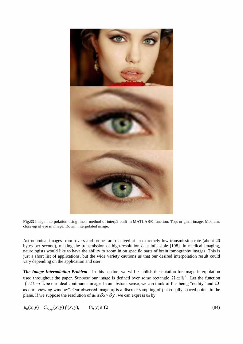
Fig.33 Image interpolation using linear method of interp2 built-in MATLAB® function. Top: original image. Medium:

close-up of eye in image. Down: interpolated image.

Astronomical images from rovers and probes are received at an extremely low transmission rate (about 40

bytes per second), making the transmission of high-resolution data infeasible [198]. In medical imaging,

neurologists would like to have the ability to zoom in on specific parts of brain tomography images. This is

just a short list of applications, but the wide variety cautions us that our desired interpolation result could

vary depending on the application and user.

The Image Interpolation Problem - In this section, we will establish the notation for image interpolation

used throughout the paper. Suppose our image is defined over some rectangle 2 . Let the function

f : be our ideal continuous image. In an abstract sense, we can think of f as being “reality” and

as our “viewing window”. Our observed image u0 is a discrete sampling of f at equally spaced points in the

plane. If we suppose the resolution of u0 is yx , we can express u0 by

),(),,(),(),( ,0 yxyxfyxCyxu yx (84)

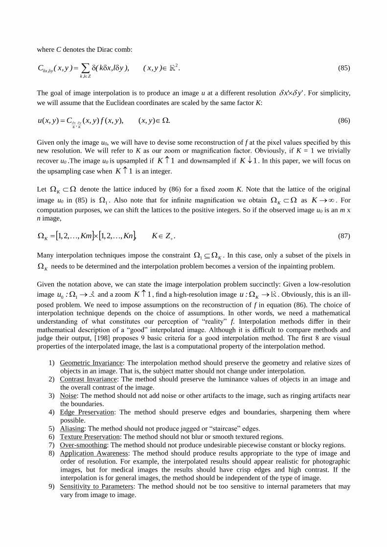
where C denotes the Dirac comb:

2

x, y

k ,l Z

C ( x, y ) ( k x,l y ), ( x, y ) .

(85)

The goal of image interpolation is to produce an image u at a different resolution '' yx . For simplicity,

we will assume that the Euclidean coordinates are scaled by the same factor K:

.),(),,(),(),(,

yxyxfyxCyxuK

y

K

x (86)

Given only the image u0, we will have to devise some reconstruction of f at the pixel values specified by this

new resolution. We will refer to K as our zoom or magnification factor. Obviously, if K = 1 we trivially

recover u0 .The image u0 is upsampled if 1K and downsampled if 1K . In this paper, we will focus on

the upsampling case when 1K is an integer.

Let K denote the lattice induced by (86) for a fixed zoom K. Note that the lattice of the original

image u0 in (85) is 1 . Also note that for infinite magnification we obtain K as K . For

computation purposes, we can shift the lattices to the positive integers. So if the observed image u0 is an m x

n image,

.,,,2,1,,2,1 ZKKnKmK (87)

Many interpolation techniques impose the constraint K1 . In this case, only a subset of the pixels in

K needs to be determined and the interpolation problem becomes a version of the inpainting problem.

Given the notation above, we can state the image interpolation problem succinctly: Given a low-resolution

image 0 1u : and a zoom 1K , find a high-resolution image Ku : . Obviously, this is an ill-

posed problem. We need to impose assumptions on the reconstruction of f in equation (86). The choice of

interpolation technique depends on the choice of assumptions. In other words, we need a mathematical

understanding of what constitutes our perception of “reality” f. Interpolation methods differ in their

mathematical description of a “good” interpolated image. Although it is difficult to compare methods and

judge their output, [198] proposes 9 basic criteria for a good interpolation method. The first 8 are visual

properties of the interpolated image, the last is a computational property of the interpolation method.

1) Geometric Invariance: The interpolation method should preserve the geometry and relative sizes of

objects in an image. That is, the subject matter should not change under interpolation.

2) Contrast Invariance: The method should preserve the luminance values of objects in an image and

the overall contrast of the image.

3) Noise: The method should not add noise or other artifacts to the image, such as ringing artifacts near

the boundaries.

4) Edge Preservation: The method should preserve edges and boundaries, sharpening them where

possible.

5) Aliasing: The method should not produce jagged or “staircase” edges.

6) Texture Preservation: The method should not blur or smooth textured regions.

7) Over-smoothing: The method should not produce undesirable piecewise constant or blocky regions.

8) Application Awareness: The method should produce results appropriate to the type of image and

order of resolution. For example, the interpolated results should appear realistic for photographic

images, but for medical images the results should have crisp edges and high contrast. If the

interpolation is for general images, the method should be independent of the type of image.

9) Sensitivity to Parameters: The method should not be too sensitive to internal parameters that may

vary from image to image.

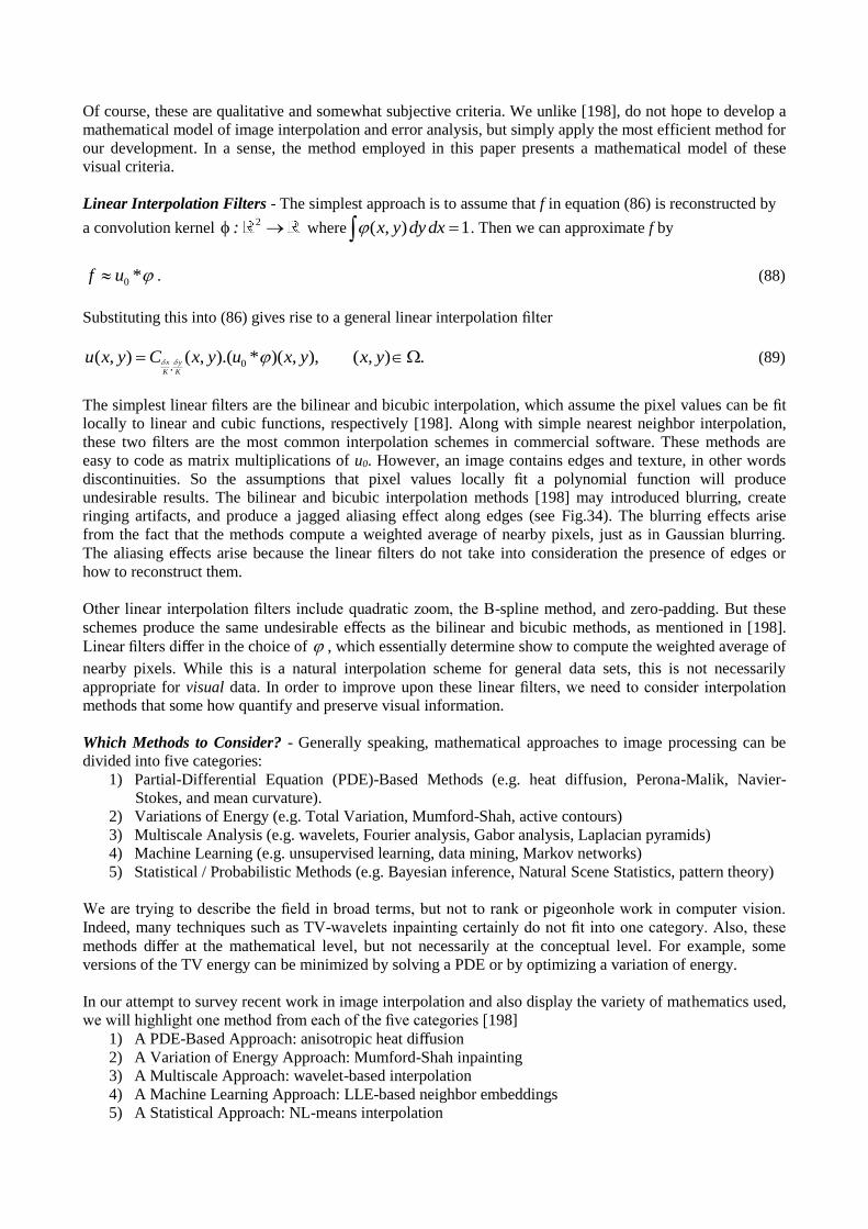
Of course, these are qualitative and somewhat subjective criteria. We unlike [198], do not hope to develop a

mathematical model of image interpolation and error analysis, but simply apply the most efficient method for

our development. In a sense, the method employed in this paper presents a mathematical model of these

visual criteria.

Linear Interpolation Filters - The simplest approach is to assume that f in equation (86) is reconstructed by

a convolution kernel 2: where 1),( dxdyyx . Then we can approximate f by

*0uf . (88)

Substituting this into (86) gives rise to a general linear interpolation filter

.),(),,)(*).(,(),( 0, yxyxuyxCyxu

K

y

K

x (89)

The simplest linear filters are the bilinear and bicubic interpolation, which assume the pixel values can be fit

locally to linear and cubic functions, respectively [198]. Along with simple nearest neighbor interpolation,

these two filters are the most common interpolation schemes in commercial software. These methods are

easy to code as matrix multiplications of u0. However, an image contains edges and texture, in other words

discontinuities. So the assumptions that pixel values locally fit a polynomial function will produce

undesirable results. The bilinear and bicubic interpolation methods [198] may introduced blurring, create

ringing artifacts, and produce a jagged aliasing effect along edges (see Fig.34). The blurring effects arise

from the fact that the methods compute a weighted average of nearby pixels, just as in Gaussian blurring.

The aliasing effects arise because the linear filters do not take into consideration the presence of edges or

how to reconstruct them.

Other linear interpolation filters include quadratic zoom, the B-spline method, and zero-padding. But these

schemes produce the same undesirable effects as the bilinear and bicubic methods, as mentioned in [198].

Linear filters differ in the choice of , which essentially determine show to compute the weighted average of

nearby pixels. While this is a natural interpolation scheme for general data sets, this is not necessarily

appropriate for visual data. In order to improve upon these linear filters, we need to consider interpolation

methods that some how quantify and preserve visual information.

Which Methods to Consider? - Generally speaking, mathematical approaches to image processing can be

divided into five categories:

1) Partial-Differential Equation (PDE)-Based Methods (e.g. heat diffusion, Perona-Malik, Navier-

Stokes, and mean curvature).

2) Variations of Energy (e.g. Total Variation, Mumford-Shah, active contours)

3) Multiscale Analysis (e.g. wavelets, Fourier analysis, Gabor analysis, Laplacian pyramids)

4) Machine Learning (e.g. unsupervised learning, data mining, Markov networks)

5) Statistical / Probabilistic Methods (e.g. Bayesian inference, Natural Scene Statistics, pattern theory)

We are trying to describe the field in broad terms, but not to rank or pigeonhole work in computer vision.

Indeed, many techniques such as TV-wavelets inpainting certainly do not fit into one category. Also, these

methods differ at the mathematical level, but not necessarily at the conceptual level. For example, some

versions of the TV energy can be minimized by solving a PDE or by optimizing a variation of energy.

In our attempt to survey recent work in image interpolation and also display the variety of mathematics used,

we will highlight one method from each of the five categories [198]

1) A PDE-Based Approach: anisotropic heat diffusion

2) A Variation of Energy Approach: Mumford-Shah inpainting

3) A Multiscale Approach: wavelet-based interpolation

4) A Machine Learning Approach: LLE-based neighbor embeddings

5) A Statistical Approach: NL-means interpolation

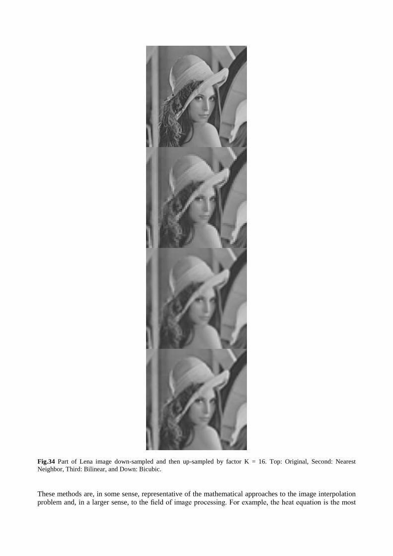
Fig.34 Part of Lena image down-sampled and then up-sampled by factor K = 16. Top: Original, Second: Nearest

Neighbor, Third: Bilinear, and Down: Bicubic.

These methods are, in some sense, representative of the mathematical approaches to the image interpolation

problem and, in a larger sense, to the field of image processing. For example, the heat equation is the most

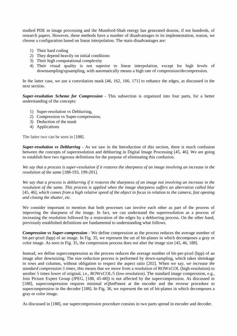
studied PDE in image processing and the Mumford-Shah energy has generated dozens, if not hundreds, of

research papers. However, these methods have a number of disadvantages to its implementation, reason, we

choose a configuration based on linear interpolation. The main disadvantages are:

1) Their hard coding

2) They depend heavily on initial conditions

3) Their high computational complexity

4) Their visual quality is not superior to linear interpolation, except for high levels of

downsampling/upsampling, with automatically means a high rate of compression/decompression.

In the latter case, we use a convolution mask [46, 162, 166, 171] to enhance the edges, as discussed in the

next section.

Super-resolution Scheme for Compression - This subsection is organized into four parts, for a better

understanding of the concepts:

1) Super-resolution vs Deblurring,

2) Compression vs Super-compression,

3) Deduction of the mask

4) Applications

The latter two can be seen in [188].

Super-resolution vs Deblurring - As we saw in the Introduction of this section, there is much confusion

between the concepts of superresolution and deblurring in Digital Image Processing [45, 46]. We are going

to establish here two rigorous definitions for the purpose of eliminating this confusion.

We say that a process is super-resolution if it restores the sharpness of an image involving an increase in the

resolution of the same [188-193, 199-201].

We say that a process is deblurring if it restores the sharpness of an image not involving an increase in the

resolution of the same. This process is applied when the image sharpness suffers an aberration called blur

[45, 46], which comes from a high relative speed of the object in focus in relation to the camera, fast opening

and closing the shutter, etc.

We consider important to mention that both processes can involve each other as part of the process of

improving the sharpness of the image. In fact, we can understand the superresolution as a process of

increasing the resolution followed by a restoration of the edges by a deblurring process. On the other hand,

previously established definitions are fundamental to understanding what follows.

Compression vs Super-compression - We define compression as the process reduces the average number of

bit-per-pixel (bpp) of an image. In Fig. 35, we represent the set of bit-planes in which decomposes a gray or

color image. As seen in Fig. 35, the compression process does not alter the image size [45, 46, 188].

Instead, we define supercompression as the process reduces the average number of bit-per-pixel (bpp) of an

image after downsizing. The size reduction process is performed by down-sampling, which takes shrinkage

in rows and columns, without obligation to respect the aspect ratio [202]. When we say, we increase the

standard compression 5 times, this means that we move from a resolution of ROWxCOL (high-resolution) to

another 5 times lower of original, i.e., ROWxCOL/5 (low-resolution). The standard image compression, e.g.,

Join Picture Expert Group (JPEG, [188, 45-48]) is not affected by the supercompression. As discussed in

[188], supercompression requires minimal eQImPment at the encoder and the reverse procedure to

supercompression in the decoder [188]. In Fig. 36, we represent the set of bit-planes in which decomposes a

gray or color image.

As discussed in [188], our supercompression procedure consists in two parts spread in encoder and decoder.

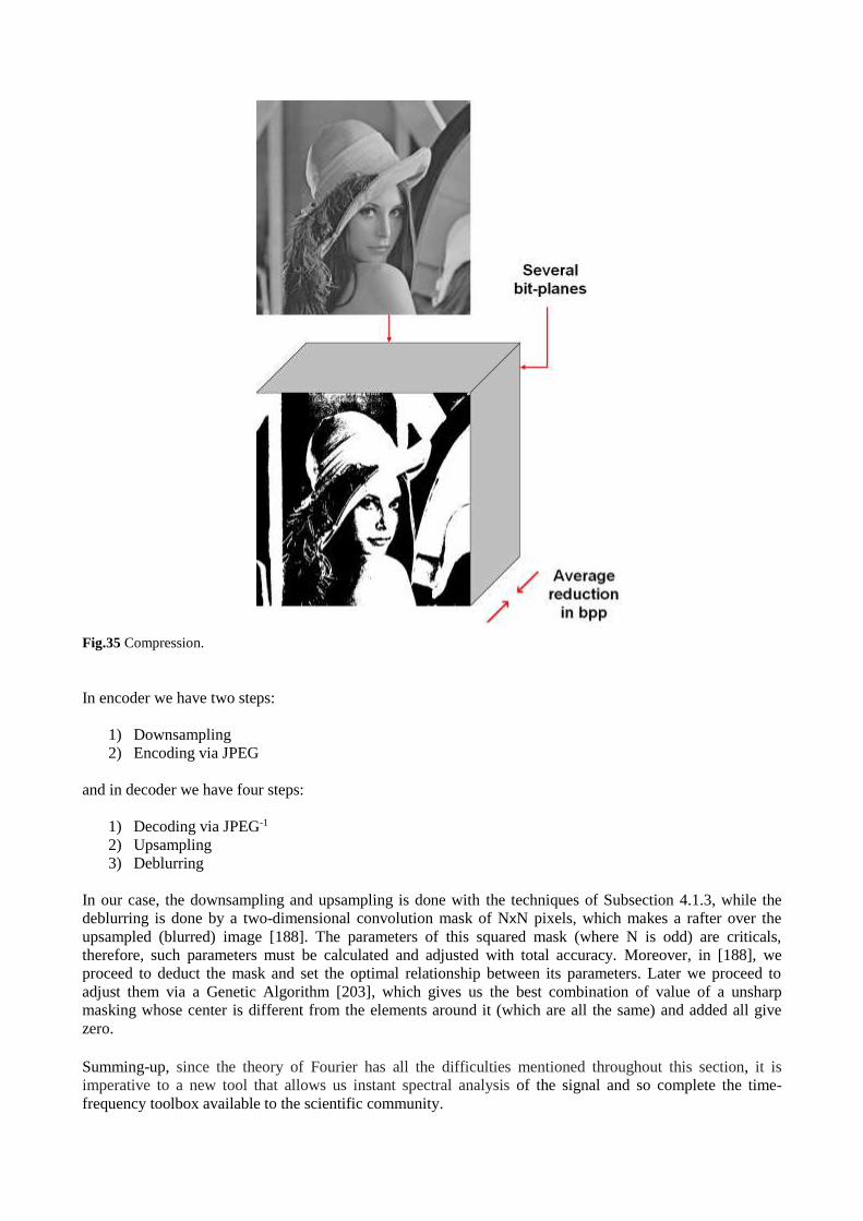
Fig.35 Compression.

In encoder we have two steps:

1) Downsampling

2) Encoding via JPEG

and in decoder we have four steps:

1) Decoding via JPEG-1

2) Upsampling

3) Deblurring

In our case, the downsampling and upsampling is done with the techniques of Subsection 4.1.3, while the

deblurring is done by a two-dimensional convolution mask of NxN pixels, which makes a rafter over the

upsampled (blurred) image [188]. The parameters of this squared mask (where N is odd) are criticals,

therefore, such parameters must be calculated and adjusted with total accuracy. Moreover, in [188], we

proceed to deduct the mask and set the optimal relationship between its parameters. Later we proceed to

adjust them via a Genetic Algorithm [203], which gives us the best combination of value of a unsharp

masking whose center is different from the elements around it (which are all the same) and added all give

zero.

Summing-up, since the theory of Fourier has all the difficulties mentioned throughout this section, it is

imperative to a new tool that allows us instant spectral analysis of the signal and so complete the time-

frequency toolbox available to the scientific community.

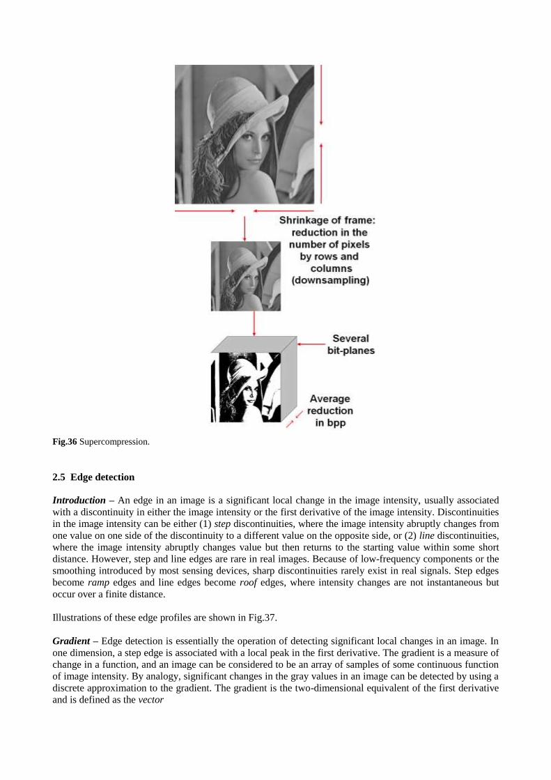
Fig.36 Supercompression.

2.5 Edge detection

Introduction – An edge in an image is a significant local change in the image intensity, usually associated

with a discontinuity in either the image intensity or the first derivative of the image intensity. Discontinuities

in the image intensity can be either (1) step discontinuities, where the image intensity abruptly changes from

one value on one side of the discontinuity to a different value on the opposite side, or (2) line discontinuities,

where the image intensity abruptly changes value but then returns to the starting value within some short

distance. However, step and line edges are rare in real images. Because of low-frequency components or the

smoothing introduced by most sensing devices, sharp discontinuities rarely exist in real signals. Step edges

become ramp edges and line edges become roof edges, where intensity changes are not instantaneous but

occur over a finite distance.

Illustrations of these edge profiles are shown in Fig.37.

Gradient – Edge detection is essentially the operation of detecting significant local changes in an image. In

one dimension, a step edge is associated with a local peak in the first derivative. The gradient is a measure of

change in a function, and an image can be considered to be an array of samples of some continuous function

of image intensity. By analogy, significant changes in the gray values in an image can be detected by using a

discrete approximation to the gradient. The gradient is the two-dimensional equivalent of the first derivative

and is defined as the vector

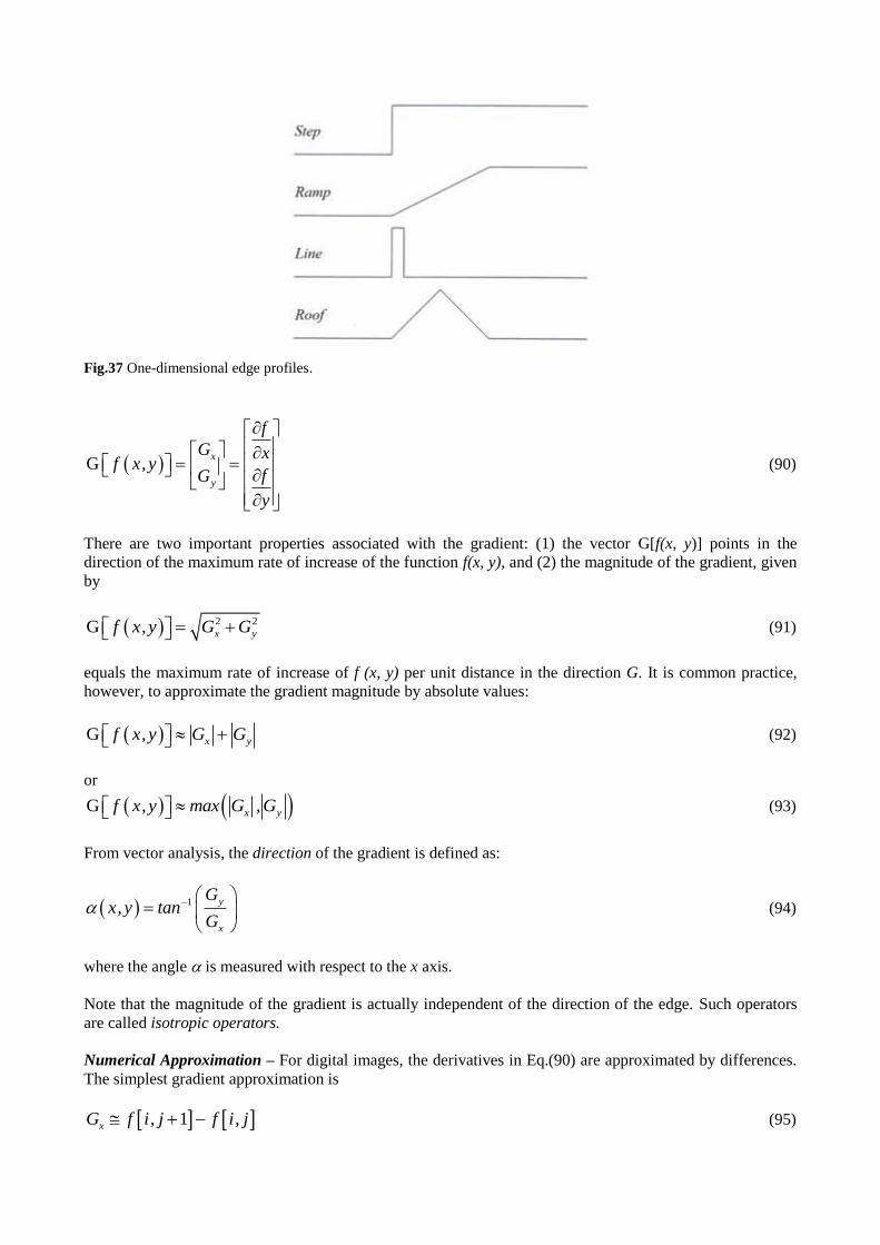
Fig.37 One-dimensional edge profiles.

Gx

y

f

G xf x, y

fG

y

(90)

There are two important properties associated with the gradient: (1) the vector G[f(x, y)] points in the

direction of the maximum rate of increase of the function f(x, y), and (2) the magnitude of the gradient, given

by

2 2G x yf x, y G G (91)

equals the maximum rate of increase of f (x, y) per unit distance in the direction G. It is common practice,

however, to approximate the gradient magnitude by absolute values:

G x yf x, y G G (92)

or

G x yf x, y max G , G (93)

From vector analysis, the direction of the gradient is defined as:

1 y

x

Gx,y tan

G

(94)

where the angle is measured with respect to the x axis.

Note that the magnitude of the gradient is actually independent of the direction of the edge. Such operators

are called isotropic operators.

Numerical Approximation – For digital images, the derivatives in Eq.(90) are approximated by differences.

The simplest gradient approximation is

1xG f i, j f i, j (95)

1yG f i, j f i , j (96)

Remember that j corresponds to the x direction and i to the negative y direction. These can be implemented

with simple convolution masks as shown below:

1

1 11

x yG G

(97)

When computing an approximation to the gradient, it is critical that the x and y partial derivatives be

computed at exactly the same position in space. However, using the above approximations, Gx is actually the

approximation to the gradient at the interpolated point [i, j+1/2] and Gy at [i+1/2, j]. For this reason, 2 x 2

first differences, rather than 2 x 1 and 1 x 2 masks, are often used for the x and y partial derivatives:

1 1 1 1

1 1 1 1x yG G

(98)

Now, the positions about which the gradients in the x and y directions are calculated are the same. This point

lies between all four pixels in the 2 x 2 neighborhood at the interpolated point [i+1/2, j+1/2]. This fact may

lead to some confusion. Therefore, an alternative approach is to use a 3 x 3 neighborhood and calculate the

gradient about the center pixel. These methods are discussed next.

Steps in edge detection – Algorithms for edge detection contain three steps:

- Filtering: Since gradient computation based on intensity values of only two points are susceptible to

noise and other vagaries in discrete computations, filtering is commonly used to improve the

performance of an edge detector with respect to noise. However, there is a trade-off between edge

strength and noise reduction. More filtering to reduce noise results in a loss of edge strength.

- Enhancement: In order to facilitate the detection of edges, it is essential to determine changes in

intensity in the neighborhood of a point. Enhancement emphasizes pixels where there is a significant

change in local intensity values and is usually performed by computing the gradient magnitude.

- Detection: We only want points with strong edge content. However, many points in an image have a

nonzero value for the gradient, and not all of these points are edges for a particular application.

Therefore, some method should be used to determine which points are edge points. Frequently,

thresholding provides the criterion used for detection.

- Localization: The location of the edge can be estimated with subpixel resolution if required for the

application. The edge orientation can also be estimated.

Roberts Operator – The Roberts cross operator provides a simple approximation to the gradient magnitude

(above view):

G 1 1 1 1f i, j f i, j f i , j f i , j f i, j (99)

Using convolution masks, this becomes

G x yf i, j G G (100)

where Gx and Gy are calculated using the following masks:

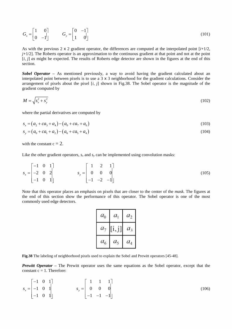
1 0 0 1

0 1 1 0x yG G

(101)

As with the previous 2 x 2 gradient operator, the differences are computed at the interpolated point [i+1/2,

j+1/2]. The Roberts operator is an approximation to the continuous gradient at that point and not at the point

[i, j] as might be expected. The results of Roberts edge detector are shown in the figures at the end of this

section.

Sobel Operator – As mentioned previously, a way to avoid having the gradient calculated about an

interpolated point between pixels is to use a 3 x 3 neighborhood for the gradient calculations. Consider the

arrangement of pixels about the pixel [i, j] shown in Fig.38. The Sobel operator is the magnitude of the

gradient computed by

2 2

x yM s s (102)

where the partial derivatives are computed by

2 3 4 0 7 6xs a ca a a ca a (103)

0 1 2 6 5 4ys a ca a a ca a (104)

with the constant c = 2.

Like the other gradient operators, sx and sy can be implemented using convolution masks:

1 0 1 1 2 1

2 0 2 0 0 0

1 0 1 1 2 1

x ys s

(105)

Note that this operator places an emphasis on pixels that are closer to the center of the mask. The figures at

the end of this section show the performance of this operator. The Sobel operator is one of the most

commonly used edge detectors.

Fig.38 The labeling of neighborhood pixels used to explain the Sobel and Prewitt operators [45-48].

Prewitt Operator – The Prewitt operator uses the same equations as the Sobel operator, except that the

constant c = 1. Therefore:

1 0 1 1 1 1

1 0 1 0 0 0

1 0 1 1 1 1

x ys s

(106)

Note that, unlike the Sobel operator, this operator does not place any emphasis on pixels that are closer to the

center of the masks. The performance of this edge detector is also shown in the figures at the end of this

section.

Canny Edge Detector – The Canny edge detector is the first derivative of a Gaussian and closely

approximates the operator that optimizes the product of signal-to-noise ratio and localization. The Canny

edge detection algorithm is summarized by the following notation. Let I[i, j] denote the image. The result

from convolving the image with a Gaussian smoothing filter using separable filtering is an array of smoothed

data,

S i, j G i, j; I i, j (107)

where is the spread of the Gaussian and controls the degree of smoothing. The gradient of the smoothed

array S[i, j] can be computed using the 2 x 2 first-difference approximations (Subsection relating to Gradient)

to produce two arrays P[i, j] and Q[i, j] for the x and y partial derivatives:

1 1 1 1 2P i, j S i, j S i, j S i , j S i , j / (108)

1 1 1 1 2Q i, j S i, j S i , j S i, j S i , j / (109)

The finite differences are averaged over the 2 x 2 square so that the x and y partial derivatives are computed

at the same point in the image. The magnitude and orientation of the gradient can be computed from the

standard formulas for rectangular-to-polar conversion:

2 2

M i, j P i, j Q i, j (110)

i, j arctan Q i, j ,P i, j (111)

where the arctan function takes two arguments and generates an angle over the entire circle of possible

directions. These functions must be computed efficiently, preferably without using floating-point arithmetic

[45-48]. Finally, the Canny Edge Detection Algorithm is:

- Smooth the image with a Gaussian filter.

- Compute the gradient magnitude and orientation using finite-difference approximations for

the partial derivatives.

- Apply nonmaxima suppression to the gradient magnitude.

- Use the double thresholding algorithm to detect and link edges.

To see in detail the items of the algorithm, we recommend reading Chapter 5 of [204].

In Fig.39, we can see original image of Agus in Miami (top), Roberts (middle-left), Sobel (middle-right),

Prewitt (down-left), and finally, Canny (down-right).

In [204], the authors compare the different edge detectors discussed so far. The comparisons are presented

according to the first three steps described at the beginning of this section: filtering, enhancement, and

detection. The estimation step is not be shown there. In addition, They give results of edge detection on

noisy images for two specific cases-one utilizing the filtering step and one omitting the filtering step. Results

of edge detection using varying amounts of filtering are also be given. In fact, shows results of all the edge

detection methods discussed so far, from the simple 1 x 2 gradient approximation up to the Prewitt operator.

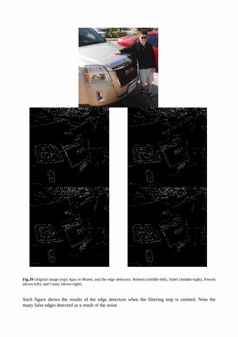
Fig.39 Original image (top) Agus in Miami, and the edge detectors: Roberts (middle-left), Sobel (middle-right), Prewitt

(down-left), and Canny (down-right).

Such figure shows the results of the edge detectors when the filtering step is omitted. Note the

many false edges detected as a result of the noise.

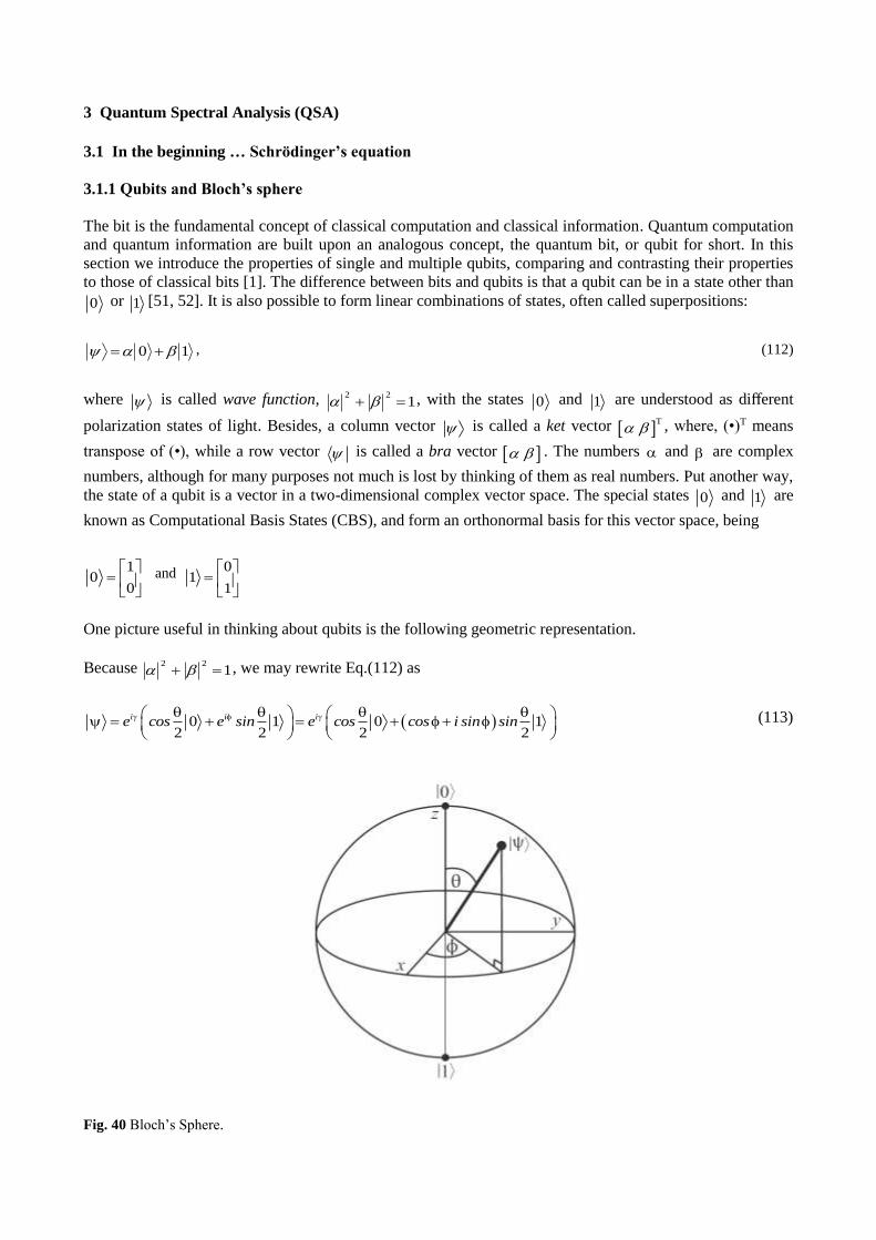
3 Quantum Spectral Analysis (QSA)

3.1 In the beginning … Schrödinger’s equation

3.1.1 Qubits and Bloch’s sphere

The bit is the fundamental concept of classical computation and classical information. Quantum computation

and quantum information are built upon an analogous concept, the quantum bit, or qubit for short. In this

section we introduce the properties of single and multiple qubits, comparing and contrasting their properties

to those of classical bits [1]. The difference between bits and qubits is that a qubit can be in a state other than

0 or 1 [51, 52]. It is also possible to form linear combinations of states, often called superpositions:

10 , (112)

where is called wave function, 1

22 , with the states 0 and 1 are understood as different

polarization states of light. Besides, a column vector is called a ket vector T

, where, (•)T means

transpose of (•), while a row vector is called a bra vector . The numbers and are complex

numbers, although for many purposes not much is lost by thinking of them as real numbers. Put another way,

the state of a qubit is a vector in a two-dimensional complex vector space. The special states 0 and 1 are

known as Computational Basis States (CBS), and form an orthonormal basis for this vector space, being

1

00

and 01

1

One picture useful in thinking about qubits is the following geometric representation.

Because 122 , we may rewrite Eq.(112) as

0 1 0 12 2 2 2

i i ie cos e sin e cos cos i sin sin

(113)

Fig. 40 Bloch’s Sphere.

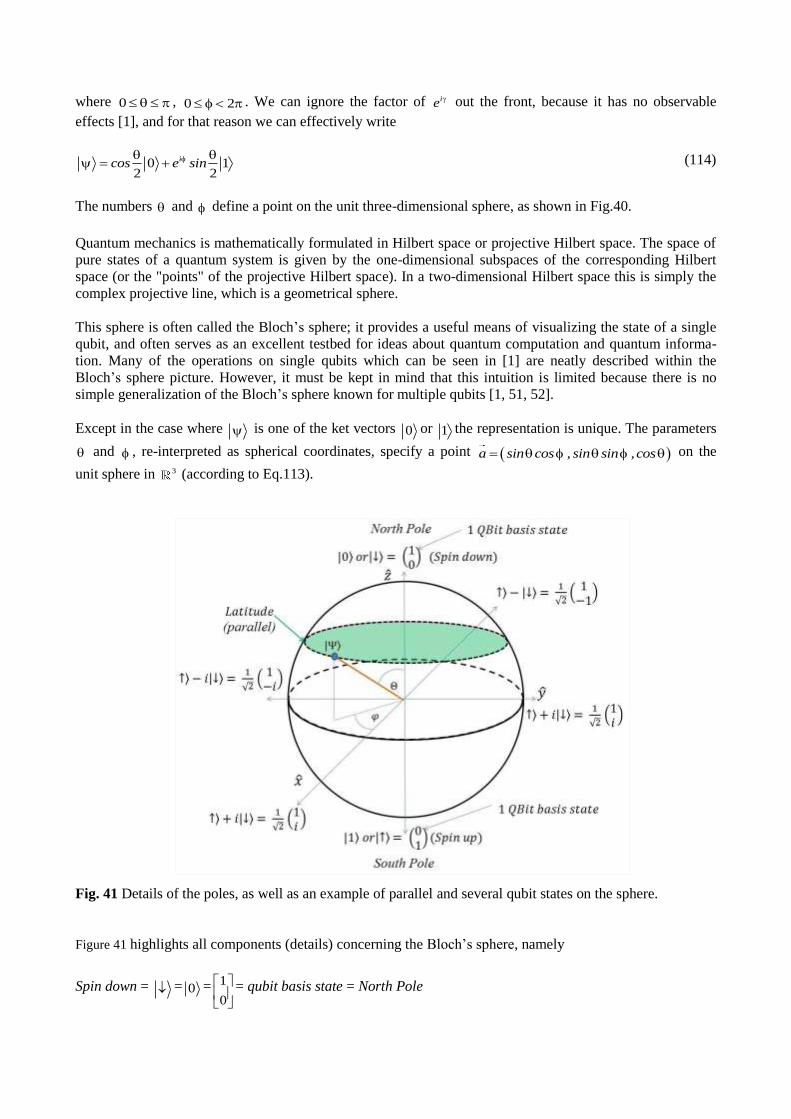
where 0 , 0 2 . We can ignore the factor of ie out the front, because it has no observable

effects [1], and for that reason we can effectively write

0 12 2

icos e sin (114)

The numbers and define a point on the unit three-dimensional sphere, as shown in Fig.40.

Quantum mechanics is mathematically formulated in Hilbert space or projective Hilbert space. The space of

pure states of a quantum system is given by the one-dimensional subspaces of the corresponding Hilbert

space (or the "points" of the projective Hilbert space). In a two-dimensional Hilbert space this is simply the

complex projective line, which is a geometrical sphere.

This sphere is often called the Bloch’s sphere; it provides a useful means of visualizing the state of a single

qubit, and often serves as an excellent testbed for ideas about quantum computation and quantum informa-

tion. Many of the operations on single qubits which can be seen in [1] are neatly described within the

Bloch’s sphere picture. However, it must be kept in mind that this intuition is limited because there is no

simple generalization of the Bloch’s sphere known for multiple qubits [1, 51, 52].

Except in the case where is one of the ket vectors 0 or 1 the representation is unique. The parameters

and , re-interpreted as spherical coordinates, specify a point a sin cos , sin sin ,cos on the

unit sphere in 3 (according to Eq.113).

Fig. 41 Details of the poles, as well as an example of parallel and several qubit states on the sphere.

Figure 41 highlights all components (details) concerning the Bloch’s sphere, namely

Spin down = = 0 = 1

0

= qubit basis state = North Pole

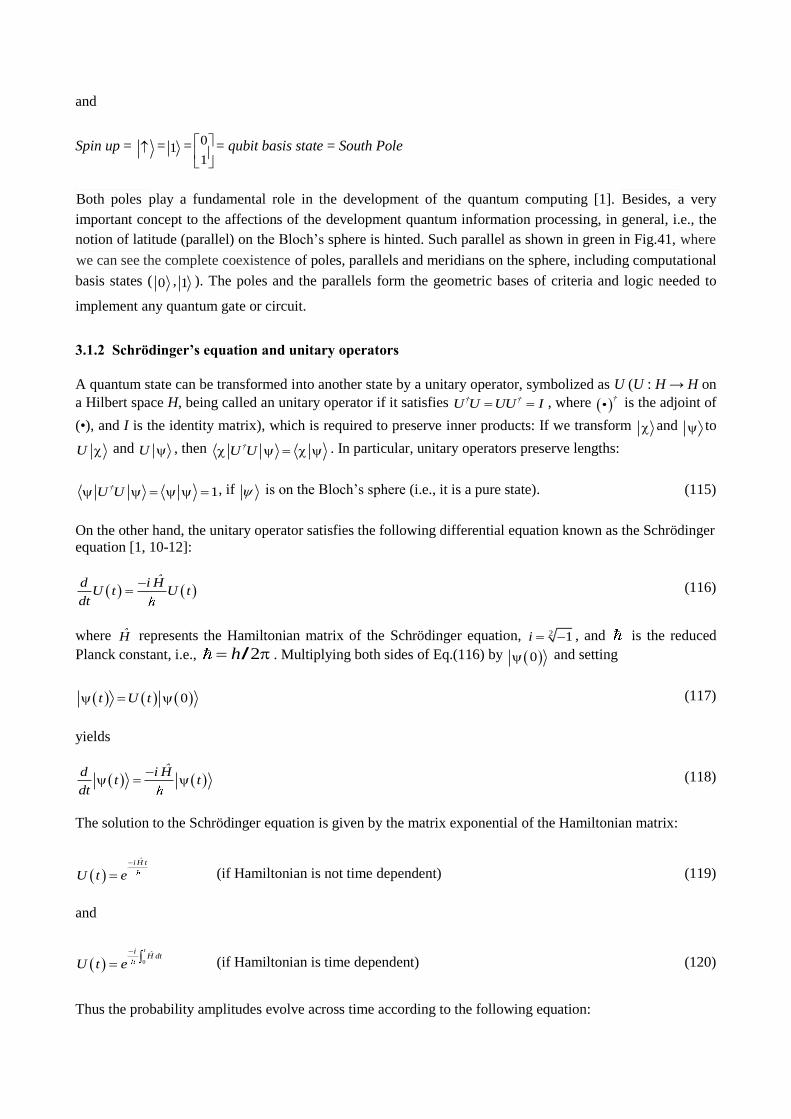
and

Spin up = = 1 = 0

1

= qubit basis state = South Pole

Both poles play a fundamental role in the development of the quantum computing [1]. Besides, a very

important concept to the affections of the development quantum information processing, in general, i.e., the

notion of latitude (parallel) on the Bloch’s sphere is hinted. Such parallel as shown in green in Fig.41, where

we can see the complete coexistence of poles, parallels and meridians on the sphere, including computational

basis states ( 0 , 1 ). The poles and the parallels form the geometric bases of criteria and logic needed to

implement any quantum gate or circuit.

3.1.2 Schrödinger’s equation and unitary operators

A quantum state can be transformed into another state by a unitary operator, symbolized as U (U : H → H on

a Hilbert space H, being called an unitary operator if it satisfies † †U U UU I , where †

• is the adjoint of

(•), and I is the identity matrix), which is required to preserve inner products: If we transform and to

U and U , then †U U . In particular, unitary operators preserve lengths:

1†U U , if is on the Bloch’s sphere (i.e., it is a pure state). (115)

On the other hand, the unitary operator satisfies the following differential equation known as the Schrödinger

equation [1, 10-12]:

ˆd i H

U t U tdt

(116)

where H represents the Hamiltonian matrix of the Schrödinger equation, 2 1i , and is the reduced

Planck constant, i.e., 2h / . Multiplying both sides of Eq.(116) by 0 and setting

0t U t (117)

yields

ˆd i H

t tdt

(118)

The solution to the Schrödinger equation is given by the matrix exponential of the Hamiltonian matrix:

ˆi H t

U t e

(if Hamiltonian is not time dependent) (119)

and

0

tiH dt

U t e

(if Hamiltonian is time dependent) (120)

Thus the probability amplitudes evolve across time according to the following equation:

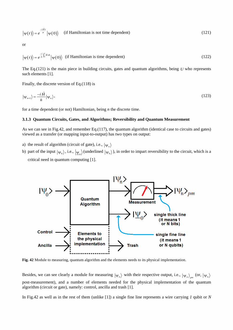
0

ˆi H t

t e

(if Hamiltonian is not time dependent) (121)

or

0 0

tiH dt

t e

(if Hamiltonian is time dependent) (122)

The Eq.(121) is the main piece in building circuits, gates and quantum algorithms, being U who represents

such elements [1].

Finally, the discrete version of Eq.(118) is

1n n

ˆi H

, (123)

for a time dependent (or not) Hamiltonian, being n the discrete time.

3.1.3 Quantum Circuits, Gates, and Algorithms; Reversibility and Quantum Measurement

As we can see in Fig.42, and remember Eq.(117), the quantum algorithm (identical case to circuits and gates)

viewed as a transfer (or mapping input-to-output) has two types on output:

a) the result of algorithm (circuit of gate), i.e.,

n

b) part of the input 0 , i.e.,

0 (underlined

0 ), in order to impart reversibility to the circuit, which is a

critical need in quantum computing [1].

Fig. 42 Module to measuring, quantum algorithm and the elements needs to its physical implementation.

Besides, we can see clearly a module for measuring n with their respective output, i.e.,

n pm (or,

n

post-measurement), and a number of elements needed for the physical implementation of the quantum

algorithm (circuit or gate), namely: control, ancilla and trash [1].

In Fig.42 as well as in the rest of them (unlike [1]) a single fine line represents a wire carrying 1 qubit or N

qubits (qudit), interchangeably, while a single thick line represents a wire carrying 1 or N classical bits,

interchangeably too. However, the mentioned concept of reversibility is closely related to energy consump-

tion, and hence to the Landauer’s Principle [1].

On the other hand, computational complexity studies the amount of time and space required to solve a

computational problem. Another important computational resource is energy. In [1], the authors show the

energy requirements for computation. Surprisingly, it turns out that computation, both classical and quantum,

can in principle be done without expending any energy! Energy consumption in computation turns out to be

deeply linked to the reversibility of the computation. In other words, it is inexcusable the need of the

0 presence to the output of quantum gate [1].

On the other hand, in quantum mechanics, measurement is a non-trivial and highly counter-intuitive process.

Firstly, because measurement outcomes are inherently probabilistic, i.e. regardless of the carefulness in the

preparation of a measurement procedure, the possible outcomes of such measurement will be distributed

according to a certain probability distribution. Secondly, once the measurement has been performed, a

quantum system in unavoidably altered due to the interaction with the measurement apparatus. Consequen-

tly, for an arbitrary quantum system, pre-measurement and post-measurement quantum states are different in

general [1].

Postulate. Quantum measurements are described by a set of measurement operators mM , index m labels

the different measurement outcomes, which act on the state space of the system being measured. Measu-

rement outcomes correspond to values of observables, such as position, energy and momentum, which are

Hermitian operators [1] corresponding to physically measurable quantities.

Let be the state of the quantum system immediately before the measurement. Then, the probability that

result m occurs is given by

†

m mˆ ˆp( m ) M M (124)

and the post-measurement quantum state is

m

pm †

m m

M

ˆ ˆM M

(125)

Operators mM must satisfy the completeness relation of Eq.(126), because that guarantees that probabilities

will sum to one; see Eq.(127) [1]:

†

m mm

ˆ ˆM M I (126)

1†

m mm m

ˆ ˆM M p( m ) (127)

Let us work out a simple example. Assume we have a polarized photon with associated polarization orienta-

tions ‘horizontal’ and ‘vertical’. The horizontal polarization direction is denoted by 0 and the vertical

polarization direction is denoted by 1 . Thus, an arbitrary initial state for our photon can be described by the

quantum state 10 (remembering Subsection 3.1.1), where and are complex numbers

constrained by the normalization condition 122 , and 0 1, is the computational basis spanning

2 .

Now, we construct two measurement operators 0 0 0M and

1 1 1M and two measurement outcomes

0 1,a a . Then, the full observable used for measurement in this experiment is 0 10 0 1 1M a a .

According to Postulate, the probabilities of obtaining outcome 0a or outcome

1a are given by 2

0p( )a

and 2

1p( )a . Corresponding post-measurement quantum states are as follows: if outcome = 0a , then

0pm

; if outcome = 1a then 1

pm .

3.2 QSA properly speaking

The Eq.(118) represents the Schrödinger equation, which we are going to write it in a better way, so as to

simplify notation

t i t t (128)

where d

t tdt

and H t

t , being the angular frequency matrix, and H the Hamiltonian

matrix. Both time dependents, simultaneously, i.e., at each instant, we will have a matrix.

On the other hand, depends on the respective –non relativistic– system, that is to say, where the most

general form for one qubit is

11 12

21 22

t tt

t t

(129)

Two interesting particular cases are represented by

1

2

0

0

tt

t

(130)

and

0 1 0

0 0 1

tt t t I t

t

(131)

being I the identity matrix. Thus, replacing Eq.(131) in Eq.(128), we will have,

t i t t . (132)

Now, we multiply both sides (by left) of Eq.(132) by t ,

t t i t t t . (133)

Finally, t results,

t tt i

t t

. (134)

Equation (134) represents QSA for the monotone case. Now, and considering Equations (128) and (129),

where represents an irreducible matrix, then, we are going to multiply both sides (by right) of Eq.(128) by

t , therefore,

t t i t t t (135)

Finally, t results,

1

†

t i t t t t

i t t

(136)

where

1

†t t t t

(is the pseudoinverse of t ) (137)

Equation (136) represents QSA for the multitone case.

3.3 Frequency in time (FIT)

Once we have arrived at the classical world, we can then apply an adaptation QSA to signals and images,

with and without overlap of samples or pixels, respectively. Such adaptation is called frequency in time

(FIT).

3.3.1 FIT for signals

Case with overlap – In the classical version of Eq.(134) we are going to replace qubits by samples of a real

signal, therefore, inner products disappear, and the classical version of Eq.(134) in a symbolic form is

1 S t S t

t i iS t t S t

, (138)

where S t

S tt

, and S is a signal defined in N , being N the size of the signal, and the frequency

(in here, while in QSA is the imaginary angular frequency).

Appealing (for simplicity) to the discrete version of , we will have,

i S. / S , (139)

where “ . / ” represents the infixed version of Hadamard’s quotient of vectors [80], 0 1 2 1NS s s s s is a

signal of N samples, 0 1 2 1NS s s s s is its derivative, and 0 1 2 1N . That is to

say, for each sample, we will have,

0 1n n ni s / s n ,N , being: 1 1 2n n ns s s / , and n the discrete time. (140)

Equation (140) is the discrete version of in its most inapplicable form, given that this is not applicable

in cases where the denominator is zero (although unlike the FFT, has solution), without mentioning that

is an imaginary operator to be applied to real signals. Therefore, this form is called raw version. To

overcome this drawback, we use equalized and/or averaged versions, as the following,

eq eq eqi S . / S , (141)

where subscript “eq“ means equalized. In general, S is equalized inside [1, 2] as follows:

- calculate maximum of S, max(S)

- calculate minimum of S, min(S)

- 1eqS S min S / max S min S

- calculate eqS

- calculate eq

While the averaged form will be,

av i S / avg S , (142)

where avg S is the average of S. In both cases the signal must be enlarged (padded). For example, we see

this in more detail in the third version,

um um umi S . / S , (143)

where the subscript um means one-dimensional mask. That is to say, in order, we will have,

0 1 2 1NS s s s s (144)

of length N, with masks of length M (odd number), and side surplus (padding) of length 1 2L ( M ) / ,

finally, we define four new elements, such as the padded S

2 1 0 1 2 1 1 2

2 1 1 2

padding L N N N L

L N N L

S s s , s s s s , s s

s s , S , s s

, (145)

of length 2 1N' N L N M , and for each 2 2n L,N L generic sample, we will have

1 1n,L n L n L n n L n Ls s s s s s , (146)

of length M. Finally, we are going to define two additional masks of length M

1 1 1 1 1 MD / , (scaling operator) (147)

and

1 1 1 0 1 1 1 M-1/ , (wavelet operator) (148)

with,

T

um,n n,Ls s D (approximation band) (149)

where superscript T means transpose, and

T

um,n n,Ls s (detail band) (150)

If M = 3, then um,ns will be the traditional discrete derivative case (see the same row of Eq.140), i.e.,

1 1 2um,n n ns s s / , while, 1 1 3um,n n n ns s s s / . These are a special case of what we have seen above.

Finally, for each sample n, we will have, the instantaneous version of Eq.(143) in term of Equations (149)

and (150),

um,n um,n um,ni s / s , (151)

0 1n ,N . On the other hand, and to save the fact that is an imaginary operator to be applied to

real signals (in all four versions), we will use (based on Eq.139) a more pure and useful version of frequency

in time (FIT) for all mentioned versions:

1

. conj

i S. / S . conj i S. / S

SS. / S S . / S

S t

(152)

Being 0 1 2 12 Nf / f f f f , the frequencies in hertz. Besides, isnow a real operator to be

applied to real signals. Remember that, this version (the original) depends on a possible denominator equal to

zero, therefore, we will use the next versions directly dependent on the frequency:

1

2

1

2

1 1

2 2

eq eq eq

eq eq eq eq

eq eq eq eq

f . conj

i S . / S . conj i S . / S

S . / S S . / S

for Eq.(141) (153)

1

2

1

2

1

2

av av avf . conj

i S . conj i S

avg S

S / avg S

for Eq.(142) (154)

and finally, one version more based on Eq.(143), that is to say,

1

2

1

2

1 1

2 2

um um um

um um um um

um um um um

f . conj

i S . / S . conj i S . / S

S . / S S . / S

(155)

Because usually a (or more) denominator of Eq.(151) is zero, then here also it is necessary to use a procedure

of equalization or normalization as in the previous cases.

Examples - Next, we will implement the four seen cases of FIT to a signal as shown in Fig.43, which is an

electrocardiographic (ECG) signal of 80 pulses per second. Top of Fig.43 shows the ECG, while its down

shows the waterfall of ECG signal, where the positive peaks are clear, the negative peaks are dark, and the

intermediates are gray.

On the other hand, Fig.44 shows the same signal of Fig.43, i.e., ECG of 80 cycles per second, with 256

samples per cycle, however, in this case, the six cells (sub-figures) contain: ECG signal in blue, and FIT in

red with their respective scales, i.e., ECG scale in blue to the left and FIT scale in red to the right. It is

important to mention that the bottom of each figure shows a sequence of witness bars. The distribution of

such witness bars is in each case the FIT itself, that is to say, the accumulation of said bars has to do with the

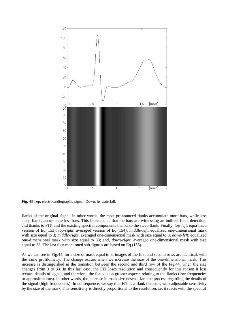
Fig. 43 Top: electrocardiographic signal. Down: its waterfall.

flanks of the original signal, in other words, the most pronounced flanks accumulate more bars, while less

steep flanks accumulate less bars. This indicates us that the bars are witnessing an indirect flank detection,

and thanks to FIT, and the existing spectral components thanks to the steep flank. Finally, top-left: equa-lized

version of Eq.(153); top-right: averaged version of Eq.(154); middle-left: equalized one-dimensional mask

with size equal to 3; middle-right: averaged one-dimensional mask with size equal to 3; down-left: equalized

one-dimensional mask with size equal to 33; and, down-right: averaged one-dimensional mask with size

equal to 33. The last four mentioned sub-figures are based on Eq.(155).

As we can see in Fig.44, for a size of mask equal to 3, images of the first and second rows are identical, with

the same profilometry. The change occurs when we increase the size of the one-dimensional mask. This

increase is distinguished in the transition between the second and third row of the Fig.44, when the size

changes from 3 to 33. In this last case, the FIT loses resolution and consequently for this reason it loss

texture details of signal, and therefore, the focus is on grosser aspects relating to the flanks (low frequencies

or approximations). In other words, the increase in mask size desensitizes the process regarding the details of

the signal (high frequencies). In consequence, we say that FIT is a flank detector, with adjustable sensitivity

by the size of the mask. This sensitivity is directly proportional to the resolution, i.e., it reacts with the spectral

Fig. 44 In all of sub-figures, we have: ECG signal in blue, and FIT in red with their respective scales, i.e., ECG scale in

blue to the left and FIT scale in red to the right. Besides, ECG signal has 80 cycles per second, with 256 samples. It is

important to mention that the bottom of each figure shows a sequence of witness bars. The distribution of such witness

bars is each case the FIT itself, that is to say, the accumulation of said bars has to do with the flanks of the original

signal, in other words, the most pronounced flanks accumulate more bars, while less steep flanks accumulate less bars.

This indicates us that the bars are witnessing an indirect flank detection, and thanks to FIT, and the existing spectral

components thanks to the steep flank. Finally, top-left: equalized version of Eq.(153); top-right: averaged version of

Eq.(154); middle-left: equalized one-dimensional mask with size equal to 3; middle-right: averaged one-dimensional

mask with size equal to 3; down-left: equalized one-dimensional mask with size equal to 33; and, down-right: averaged

one-dimensional mask with size equal to 33.

components which are represented by the degree of inclination of flanks in time. Finally, in Fig.44, we can

notice that the FIT reaches the maximum where the signal has more pronounced flanks.

A fourth version is due to a change in the Schrödinger equation, i.e., Eq.(118). We may reexpress this

equation, to first order in the infinitesimal quantity dt, as

ˆi H t dtt dt I t

I i t dt t

(156)

The operator U t dt,t I i t dt is unitary [205]; because is self-adjoint it satisfies U†U = 1 to

linear order in dt.

On the other hand, we can reexpress Eq.(140) as follow

1 1 0 12

n nn

n

s si n ,N

s

, being n the discrete time, (157)

where the signal should be padded.

With similar considerations to those carried out from Eq.(128) to (157), we arrive at

1 0 1n nn

n

s si n ,N

s

, being n the discrete time, (158)

from Eq.(156). Here, too, the signal must be padded.

The general case for the complete signal

diff i diff S / S , (159)

being diff(•) the imaginary part of numerator of Eq.(158). This function is the same built-in function diff(•) of

MATLAB® [49].

Therefore, the original FIT for this equation will be

1

2

1

2

1 1

2 2

diff diff difff . conj

i diff S . / S . conj i diff S . / S

diff S . / S diff S . / S

for Eq.(159) (160)

Here, too, this version (the original) depends on a possible denominator equal to zero, therefore, we will use

the next versions:

1

2

1

2

1 1

2 2

diff ,eq diff,eq diff,eq

eq eq eq eq

eq eq eq eq

f . conj

i diff S . / S . conj i diff S . / S

diff S . / S diff S . / S

(It is equalized like Eq.141) (161)

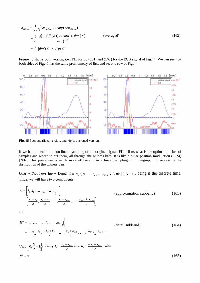
1

2

1

2

1

2

diff ,av diff ,av diff ,avf . conj

i diff S . conj i diff S

avg S

diff S / avg S

(averaged) (162)

Figure 45 shows both version, i.e., FIT for Eq.(161) and (162) for the ECG signal of Fig.44. We can see that

both sides of Fig.45 has the same profilometry of first and second row of Fig.44.

Fig. 45 Left: equalized version, and right: averaged version.

If we had to perform a non-linear sampling of the original signal, FIT tell us what is the optimal number of

samples and where to put them, all through the witness bars. It is like a pulse-position modulation (PPM)

[206]. This procedure is much more efficient than a linear sampling. Summing-up, FIT represents the

distribution of the witness bars.

Case without overlap – Being 0 1 2 1n NS s s s , s , s , 0 1n ,N , being n the discrete time.

Thus, we will have two components

1

0 11

2

0 1 2 3 1 2 1

2 2 2 2

k N

n n N N

L l , l , ,l , ,l

s s s s s s s s, , , , ,

(approximation subband) (163)

and

1

0 11

2

0 1 2 3 1 2 1

2 2 2 2

k N

n n N N

H h , h , ,h , ,h

s s s s s s s s, , , , ,

(detail subband) (164)

0 12

Nk ,

, being 1

2

n nk

s sl and 1

2

n nk

s sh , with

0L S (165)

L1 and H1 are the first level subbands of Haar basis wavelet. L1 is the approximation subband (low frequency)

and H1 is the detail subband (high frequency). L0 is the basal level or original signal. Then, QSA will be,

1 1i H . / L , (166)

while, FIT is,

1 1 1 1

1 1 1 1

1

2

1

2

1 1

2 2

f . conj

i H . / L . conj i H . / L

H . / L H . / L

(167)

As we see in the next section, it is very useful also another version of FIT for the non-overlapping case,

1 1

1

2

1

2

f abs

H . / L

(168)

where, abs(•) means absolute value of (•). On the other hand, both of them, have the same problem, i.e., they

depends on a possible denominator equal to zero, therefore, we will use the next versions:

1) Equalization: we are going to equalize S between 1 and 2 (Seq), like Eq.(141), and then, we will built 1 1

eq eqH ,L with it, i.e., eq , and hence,

1 1 1 1

1 1 1 1

1

2

1

2

1 1

2 2

eq eq eq

eq eq eq eq

eq eq eq eq

f . conj

i H . / L . conj i H . / L

H . / L H . / L

(169)

and

1 1

1

2

1

2

eq eq

eq eq

f abs

H . / L

(170)

2) Averaging: we will proceed to show this version directly starting with QSA,

1 1

av i H / avg L , (171)

Then, FIT will be,

1 1

1

1 1

1

2

1

2

1

2

av av avf . conj

i H . conj i H

avg L

H / avg L

(172)

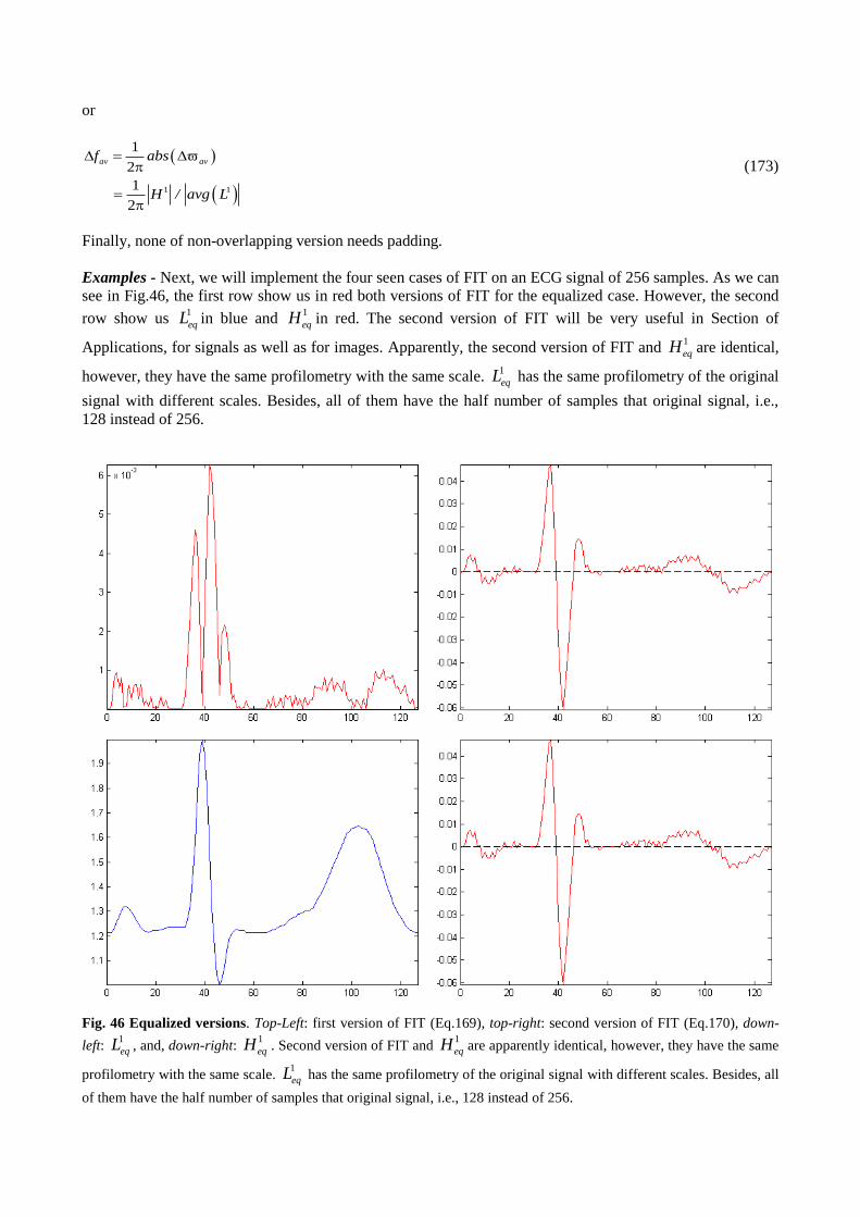
or

1 1

1

2

1

2

av avf abs

H / avg L

(173)

Finally, none of non-overlapping version needs padding.

Examples - Next, we will implement the four seen cases of FIT on an ECG signal of 256 samples. As we can

see in Fig.46, the first row show us in red both versions of FIT for the equalized case. However, the second

row show us 1

eqL in blue and 1

eqH in red. The second version of FIT will be very useful in Section of

Applications, for signals as well as for images. Apparently, the second version of FIT and 1

eqH are identical,

however, they have the same profilometry with the same scale. 1

eqL has the same profilometry of the original

signal with different scales. Besides, all of them have the half number of samples that original signal, i.e.,

128 instead of 256.

Fig. 46 Equalized versions. Top-Left: first version of FIT (Eq.169), top-right: second version of FIT (Eq.170), down-

left: 1

eqL , and, down-right: 1

eqH . Second version of FIT and 1

eqH are apparently identical, however, they have the same

profilometry with the same scale. 1

eqL has the same profilometry of the original signal with different scales. Besides, all

of them have the half number of samples that original signal, i.e., 128 instead of 256.

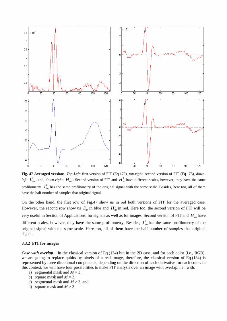
Fig. 47 Averaged versions. Top-Left: first version of FIT (Eq.172), top-right: second version of FIT (Eq.173), down-

left: 1

noL , and, down-right: 1

noH . Second version of FIT and 1

noH have different scales, however, they have the same

profilometry. 1

noL has the same profilometry of the original signal with the same scale. Besides, here too, all of them

have the half number of samples that original signal.

On the other hand, the first row of Fig.47 show us in red both versions of FIT for the averaged case.

However, the second row show us 1

noL in blue and 1

noH in red. Here too, the second version of FIT will be

very useful in Section of Applications, for signals as well as for images. Second version of FIT and 1

noH have

different scales, however, they have the same profilometry. Besides, 1

noL has the same profilometry of the

original signal with the same scale. Here too, all of them have the half number of samples that original

signal.

3.3.2 FIT for images

Case with overlap – In the classical version of Eq.(134) but in the 2D case, and for each color (i.e., RGB),

we are going to replace qubits by pixels of a real image, therefore, the classical version of Eq.(134) is

represented by three directional components, depending on the direction of each derivative for each color. In

this context, we will have four possibilities to make FIT analysis over an image with overlap, i.e., with:

a) segmental mask and M = 3,

b) square mask and M = 3,

c) segmental mask and M > 3, and

d) square mask and M > 3

In all cases, the image is padded depending on the value of M, i.e., if the image (e.g., red channel: IR) has a

ROW-by-COL size, then, IR,P (padded IR) will have a (ROW+2L)-by-(COL+2L) size, where L = (M-1)/2.

Therefore, the original image IR will be in the middle of the padded image IR,P, which will have four lateral

margins of L size to each side of IR composed exclusively by zeros.

Segmental mask and M = 3: in this case, we will have two mask, namely:

101

2HN

, (horizontal mask), and (174)

T

V HN N , (vertical mask). (175)

The procedure begins with a two-dimensional convolution (first horizontal and then, vertical rafters) between

NH and IR,P, i.e.,

H H R,PI N I (176)

After that, we continue with another two-dimensional convolution (first vertical and then, horizontal rafters)

between NV and IR,P, i.e.,

V V R,PI N I (177)

Finally, I is obtained via Pythagoras between IH , and IV , that is to say,

2 2

H VI I I (178)

Then, we obtain the two-dimensional version of Eq.(139), that is,

i I . / I , (179)

While, for each pixel, we will have,

1 1r ,c r ,c r ,ci I / I r ,ROW ,and c ,COL (180)

Equation (180) is the discrete version of in its most inapplicable form, given that this is not applicable in

cases where the denominator is zero (although unlike the FFT, has solution), without mentioning that

is an imaginary operator to be applied to real images. Therefore, this form is called raw version. To

overcome this drawback, we use equalized and/or averaged versions (like signal case), as the following,

eq eq eqi I . / I , (181)

where subscript “eq“ means equalized. In general, we will pass each pixel of each channel of color of I from

[0,28-1] to [1, 28].

While the averaged form will be,

av i I / avg I , (182)

where avg I is the average of I. In both cases the image must be enlarged (padded) as we explained before.

For example, we see this in more detail in the third version,

bm bmi I / I , (183)

where the subscript bm means two-dimensional mask.

Here too, we define two segmental mask,

111

3HD , (horizontal mask), and (184)

T

V HD D , (vertical mask). (185)

The procedure begins with a two-dimensional convolution (first horizontal and then, vertical rafters) between

DH and IR,P, i.e.,

H H R,PI D I (186)

After that, we continue with another two-dimensional convolution (first vertical and then, horizontal rafters)

between SV and IR,P, i.e.,

V V R,PI D I (187)

Finally, bmI is obtained via Pythagoras between IH , and IV , that is to say,

2 2

bm H VI I I (188)

On the other hand, and to save the fact that is an imaginary operator to be applied to real images (in all

four versions), we will use another version known as frequency in time (FIT) for all mentioned versions:

1

2

1

2

1 1

2 2

f . conj

i I . / I . conj i I . / I

I . / I I . / I

for Eq.(179) (189)

Being 2f / a matrix of ROW-by-COL frequency in hertz. Remember that, this version (the original)

depends on a possible denominator equal to zero, therefore, we will use the next versions:

1

2

1

2

1 1

2 2

eq eq eq

eq eq eq eq

eq eq eq eq

f . conj

i I . / I . conj i I . / I

I . / I I . / I

for Eq.(181) (190)

1

2

1

2

1

2

av av avf . conj

i I . conj i I

avg I

I / avg I

for Eq.(182) (191)

and finally, one version more based on Eq.(183), that is to say,

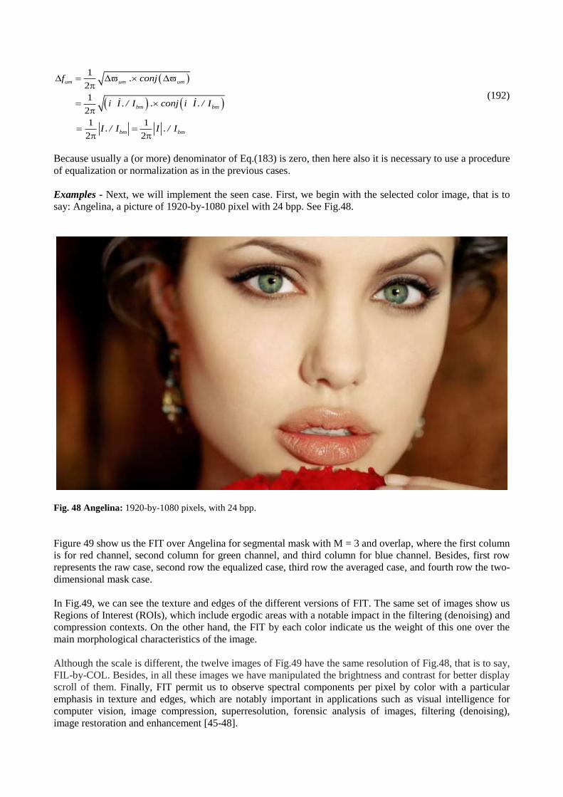
1

2

1

2

1 1

2 2

um um um

bm bm

bm bm

f . conj

i I . / I . conj i I . / I

I . / I I . / I

(192)

Because usually a (or more) denominator of Eq.(183) is zero, then here also it is necessary to use a procedure

of equalization or normalization as in the previous cases.

Examples - Next, we will implement the seen case. First, we begin with the selected color image, that is to

say: Angelina, a picture of 1920-by-1080 pixel with 24 bpp. See Fig.48.

Fig. 48 Angelina: 1920-by-1080 pixels, with 24 bpp.

Figure 49 show us the FIT over Angelina for segmental mask with M = 3 and overlap, where the first column

is for red channel, second column for green channel, and third column for blue channel. Besides, first row

represents the raw case, second row the equalized case, third row the averaged case, and fourth row the two-

dimensional mask case.

In Fig.49, we can see the texture and edges of the different versions of FIT. The same set of images show us

Regions of Interest (ROIs), which include ergodic areas with a notable impact in the filtering (denoising) and

compression contexts. On the other hand, the FIT by each color indicate us the weight of this one over the

main morphological characteristics of the image.

Although the scale is different, the twelve images of Fig.49 have the same resolution of Fig.48, that is to say,

FIL-by-COL. Besides, in all these images we have manipulated the brightness and contrast for better display

scroll of them. Finally, FIT permit us to observe spectral components per pixel by color with a particular

emphasis in texture and edges, which are notably important in applications such as visual intelligence for

computer vision, image compression, superresolution, forensic analysis of images, filtering (denoising),

image restoration and enhancement [45-48].

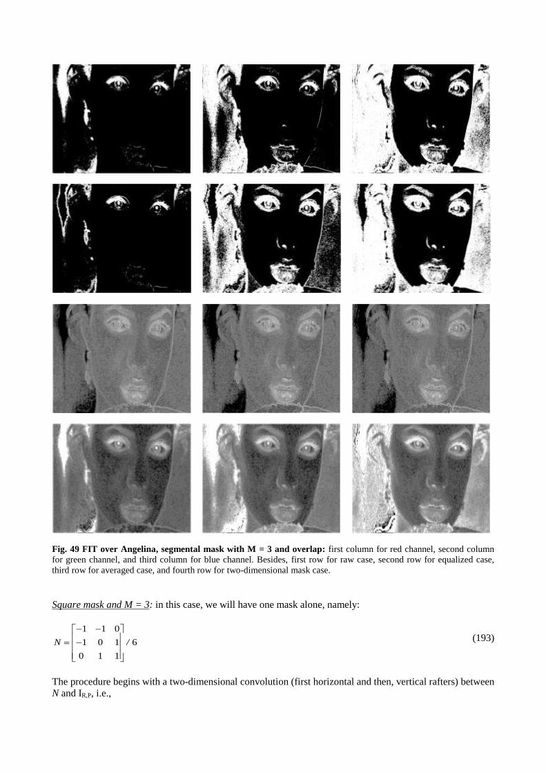
Fig. 49 FIT over Angelina, segmental mask with M = 3 and overlap: first column for red channel, second column

for green channel, and third column for blue channel. Besides, first row for raw case, second row for equalized case,

third row for averaged case, and fourth row for two-dimensional mask case.

Square mask and M = 3: in this case, we will have one mask alone, namely:

1 1 0

1 0 1 6

0 1 1

N /

(193)

The procedure begins with a two-dimensional convolution (first horizontal and then, vertical rafters) between

N and IR,P, i.e.,

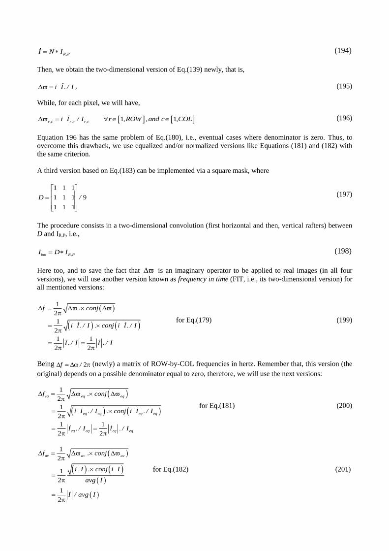
R,PI N I (194)

Then, we obtain the two-dimensional version of Eq.(139) newly, that is,

i I . / I , (195)

While, for each pixel, we will have,

1 1r ,c r ,c r ,ci I / I r ,ROW ,and c ,COL (196)

Equation 196 has the same problem of Eq.(180), i.e., eventual cases where denominator is zero. Thus, to

overcome this drawback, we use equalized and/or normalized versions like Equations (181) and (182) with

the same criterion.

A third version based on Eq.(183) can be implemented via a square mask, where

1 1 1

1 1 1 9

1 1 1

D /

(197)

The procedure consists in a two-dimensional convolution (first horizontal and then, vertical rafters) between

D and IR,P, i.e.,

bm R,PI D I (198)

Here too, and to save the fact that is an imaginary operator to be applied to real images (in all four

versions), we will use another version known as frequency in time (FIT, i.e., its two-dimensional version) for

all mentioned versions:

1

2

1

2

1 1

2 2

f . conj

i I . / I . conj i I . / I

I . / I I . / I

for Eq.(179) (199)

Being 2f / (newly) a matrix of ROW-by-COL frequencies in hertz. Remember that, this version (the

original) depends on a possible denominator equal to zero, therefore, we will use the next versions:

1

2

1

2

1 1

2 2

eq eq eq

eq eq eq eq

eq eq eq eq

f . conj

i I . / I . conj i I . / I

I . / I I . / I

for Eq.(181) (200)

1

2

1

2

1

2

av av avf . conj

i I . conj i I

avg I

I / avg I

for Eq.(182) (201)

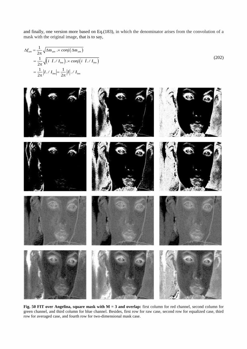
and finally, one version more based on Eq.(183), in which the denominator arises from the convolution of a

mask with the original image, that is to say,

1

2

1

2

1 1

2 2

um um um

bm bm

bm bm

f . conj

i I . / I . conj i I . / I

I . / I I . / I

(202)

Fig. 50 FIT over Angelina, square mask with M = 3 and overlap: first column for red channel, second column for

green channel, and third column for blue channel. Besides, first row for raw case, second row for equalized case, third

row for averaged case, and fourth row for two-dimensional mask case.

Here, we can make the same considerations that we make after Eq.(192) regarding to Eq.(183) and their

possible denominators equal to zero in it.

Figure 50 show us the FIT over Angelina for square mask with M = 3 and overlap, where the first column is

for red channel, second column for green channel, and third column for blue channel. Besides, first row

represents the raw case, second row the equalized case, third row the averaged case, and fourth row the two-

dimensional mask case.

Otherwise, considerations about the Fig.50 are similar to the previous case.

Fig. 51 FIT over Angelina, segmental mask with M > 3 (in fact, M = 7) and overlap: first column for red channel,

second column for green channel, and third column for blue channel. Besides, first row for raw case, second row for

equalized case, third row for averaged case, and fourth row for two-dimensional mask case.

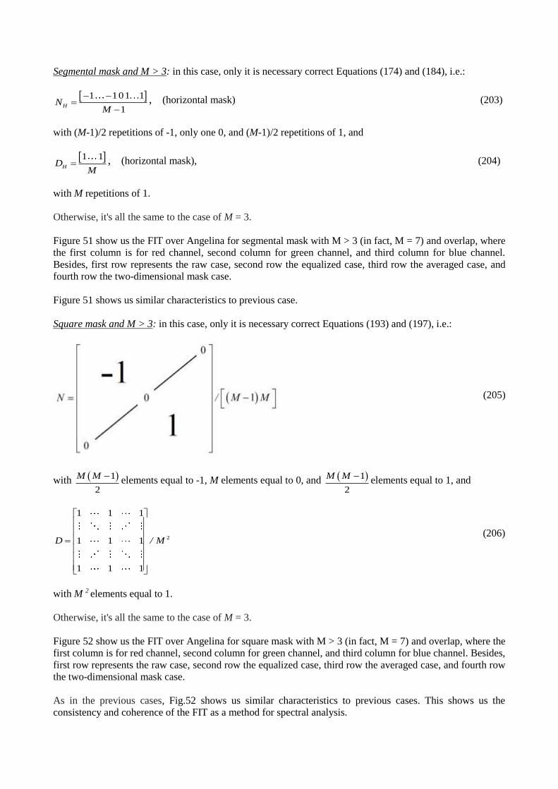
Segmental mask and M > 3: in this case, only it is necessary correct Equations (174) and (184), i.e.:

1 101 1

1HN

M

, (horizontal mask) (203)

with (M-1)/2 repetitions of -1, only one 0, and (M-1)/2 repetitions of 1, and

1 1HD

M , (horizontal mask), (204)

with M repetitions of 1.

Otherwise, it's all the same to the case of M = 3.

Figure 51 show us the FIT over Angelina for segmental mask with M > 3 (in fact, M = 7) and overlap, where

the first column is for red channel, second column for green channel, and third column for blue channel.

Besides, first row represents the raw case, second row the equalized case, third row the averaged case, and

fourth row the two-dimensional mask case.

Figure 51 shows us similar characteristics to previous case.

Square mask and M > 3: in this case, only it is necessary correct Equations (193) and (197), i.e.:

(205)

with 1

2

M M elements equal to -1, M elements equal to 0, and 1

2

M M elements equal to 1, and

2

1 1 1

1 1 1

1 1 1

D / M

(206)

with M 2 elements equal to 1.

Otherwise, it's all the same to the case of M = 3.

Figure 52 show us the FIT over Angelina for square mask with M > 3 (in fact, M = 7) and overlap, where the

first column is for red channel, second column for green channel, and third column for blue channel. Besides,

first row represents the raw case, second row the equalized case, third row the averaged case, and fourth row

the two-dimensional mask case.

As in the previous cases, Fig.52 shows us similar characteristics to previous cases. This shows us the

consistency and coherence of the FIT as a method for spectral analysis.

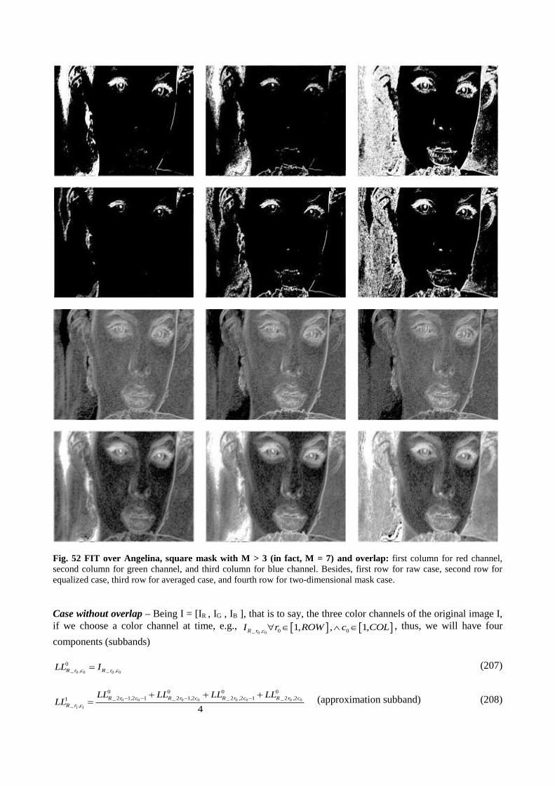
Fig. 52 FIT over Angelina, square mask with M > 3 (in fact, M = 7) and overlap: first column for red channel,

second column for green channel, and third column for blue channel. Besides, first row for raw case, second row for

equalized case, third row for averaged case, and fourth row for two-dimensional mask case.

Case without overlap – Being I = [IR , IG , IB ], that is to say, the three color channels of the original image I,

if we choose a color channel at time, e.g., 0 0 0 01 1R_r ,cI r ,ROW , c ,COL , thus, we will have four

components (subbands)

0 0 0 0

0

R _r ,c R _r ,cLL I (207)

0 0 0 0 0 0 0 0

1 1

0 0 0 0

2 1 2 1 2 1 2 2 2 1 2 21

4

R _ r , c R _ r , c R _ r , c R _ r , c

R _ r ,c

LL LL LL LLLL

(approximation subband) (208)

0 0 0 0 0 0 0 0

1 1

0 0 0 0

2 1 2 1 2 1 2 2 2 1 2 21

4

R _ r , c R _ r , c R _ r , c R _ r , c

R _ r ,c

LL LL LL LLLH

(horizontal detail subband) (209)

0 0 0 0 0 0 0 0

1 1

0 0 0 0

2 1 2 1 2 1 2 2 2 1 2 21

4

R _ r , c R _ r , c R _ r , c R _ r , c

R _ r ,c

LL LL LL LLHL

(vertical detail subband) (210)

0 0 0 0 0 0 0 0

1 1

0 0 0 0

2 1 2 1 2 1 2 2 2 1 2 21

4

R _ r , c R _ r , c R _ r , c R _ r , c

R _ r ,c

LL LL LL LLHH

(diagonal detail subband) (211)

1 11 2 1 2r ,ROW / , c ,COL /

LL1, LH1, HL1, and HH1 are the first level subbands of Haar basis wavelet for two dimensions. LL1 is the

approximation subband (low frequency), and LH1, HL1, and HH1 are the detail subbands (high frequency).

LL0 is the basal level or original image. Then QSA will be,

1 1 1

R_ H R Ri LH . / LL , (212)

1 1 1

R_V R Ri HL . / LL , (213)

1 1 1

R_ D R Ri HH . / LL , (214)

while, FIT is,

1 1 1

1 1 1 1

1 1 1 1

1

2

1

2

1 1

2 2

R _ H R _ H R _ H

R R R R

R R R R

f . conj

i LH . / LL . conj i LH . / LL

LH . / LL LH . / LL

(215)

1 1 1

1 1 1 1

1 1 1 1

1

2

1

2

1 1

2 2

R _V R _V R _V

R R R R

R R R R

f . conj

i HL . / LL . conj i HL . / LL

HL . / LL HL . / LL

(216)

1 1 1

1 1 1 1

1 1 1 1

1

2

1

2

1 1

2 2

R _ D R _ D R _ D

R R R R

R R R R

f . conj

i HH . / LL . conj i HH . / LL

HH . / LL HH . / LL

(217)

As we shall see in the next section, it is very useful also another version of FIT for the non-overlapping case,

with a subsampling to the half resolution, which is very useful for applications such as compression and

superresolution,

1 1

1 1

1

2

1

2

R _ H R _ H

R R

f abs

LH . / LL

(218)

1 1

1 1

1

2

1

2

R _V R _V

R R

f abs

HL . / LL

(219)

1 1

1 1

1

2

1

2

R _ D R _ D

R R

f abs

HH . / LL

(220)

On the other hand, all of them, have the same problem, i.e., they depends on a possible denominator equal to

zero, therefore, we will use the next versions:

Equalization: we are going to equalize IR from [0,28-1] to [1,256] (IR_eq), like Eq.(141), and then, we will

built 1 1 1 1

R_eq R_eq R_eq R_eqLL ,LH ,HL ,HH with it, i.e., 1 1 1

R_ H _eq R_V _eq R_ D_eq, , , and hence,

1 1 1

1 1 1 1

1 1 1 1

1

2

1

2

1 1

2 2

R _ H _ eq R _ H _ eq R _ H _ eq

R _ eq R _ eq R _ eq R _ eq

R _ eq R _ eq R _ eq R _ eq

f . conj

i LH . / LL . conj i LH . / LL

LH . / LL LH . / LL

(221)

1 1 1

1 1 1 1

1 1 1 1

1

2

1

2

1 1

2 2

R _V _ eq R _V _ eq R _V _ eq

R _ eq R _ eq R _ eq R _ eq

R _ eq R _ eq R _ eq R _ eq

f . conj

i HL . / LL . conj i HL . / LL

HL . / LL HL . / LL

(222)

1 1 1

1 1 1 1

1 1 1 1

1

2

1

2

1 1

2 2

R _ D _ eq R _ D _ eq R _ D _ eq

R _ eq R _ eq R _ eq R _ eq

R _ eq R _ eq R _ eq R _ eq

f . conj

i HH . / LL . conj i HH . / LL

HH . / LL HH . / LL

(223)

and

1 1

1 1

1

2

1

2

R _ H _ eq R _ H _ eq

R _ eq R _ eq

f abs

LH . / LL

(224)

1 1

1 1

1

2

1

2

R _V _ eq R _V _ eq

R _ eq R _ eq

f abs

HL . / LL

(225)

1 1

1 1

1

2

1

2

R _ D _ eq R _ D _ eq

R _ eq R _ eq

f abs

HH . / LL

(226)

Averaging: we will proceed to show this version directly starting with QSA,

1 1 1

R_ H _av R Ri LH / avg LL , (227)

1 1 1

R_V _av R Ri HL / avg LL , (228)

1 1 1

R_ D_av R Ri HH / avg LL , (229)

Then, FIT will be,

1 1 1

1 1

1

1 1

1

2

1

2

1

2

R _ H _ av R _ H _ av R _ H _ av

R R

R

R R

f . conj

i LH . conj i LH

avg LL

LH / avg LL

(230)

1 1 1

1 1

1

1 1

1

2

1

2

1

2

R _V _ av R _V _ av R _V _ av

R R

R

R R

f . conj

i HL . conj i HL

avg LL

HL / avg LL

(231)

1 1 1

1 1

1

1 1

1

2

1

2

1

2

R _ D _ av R _ D _ av R _ D _ av

R R

R

R R

f . conj

i HH . conj i HH

avg LL

HH / avg LL

(232)

or

1 1

1 1

1

2

1

2

R _ H _ av R _ H _ av

R R

f abs

LH / avg LL

(233)

1 1

1 1

1

2

1

2

R _V _ av R _V _ av

R R

f abs

HL / avg LL

(234)

1 1

1 1

1

2

1

2

R _ D _ av R _ D _ av

R R

f abs

HH / avg LL

(235)

Finally, none of non-overlapping version needs a padding over the original image, with the consequent

simplification in coding this implies.

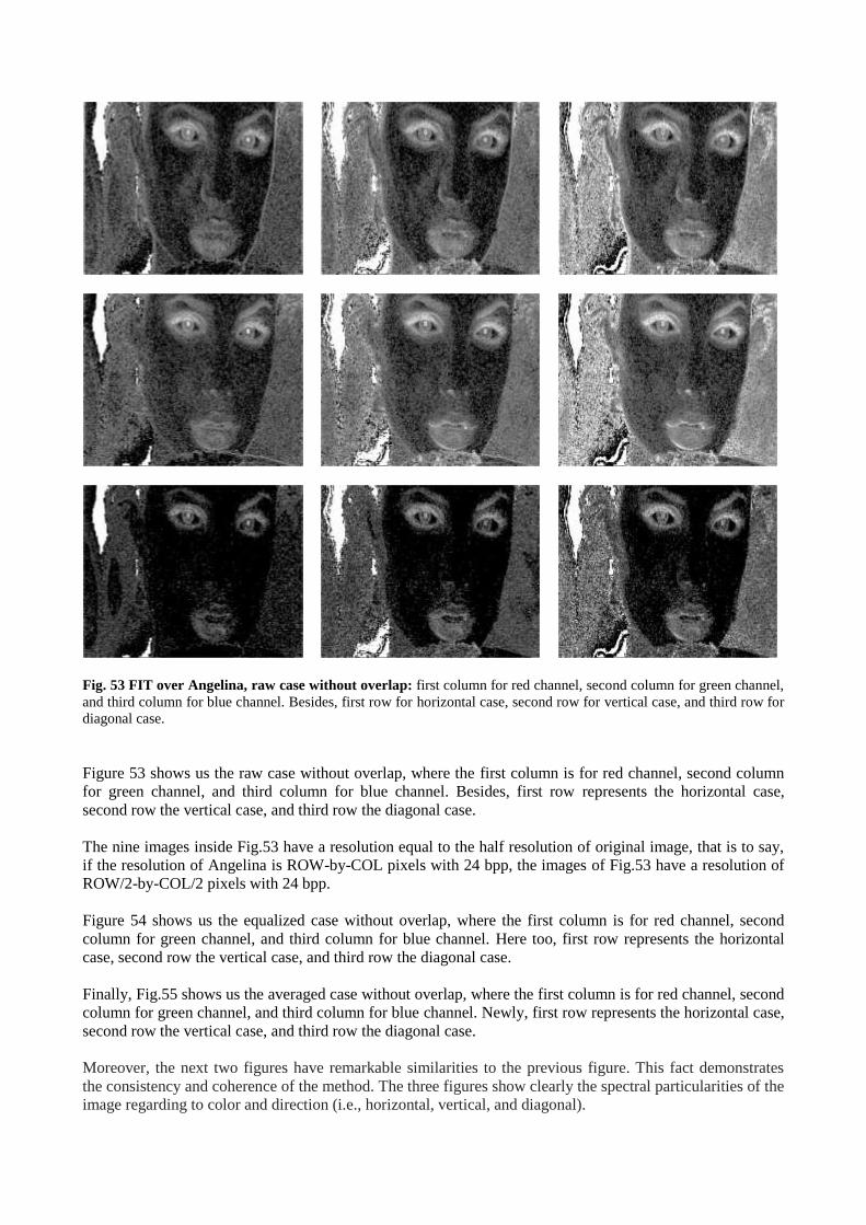
Fig. 53 FIT over Angelina, raw case without overlap: first column for red channel, second column for green channel,

and third column for blue channel. Besides, first row for horizontal case, second row for vertical case, and third row for

diagonal case.

Figure 53 shows us the raw case without overlap, where the first column is for red channel, second column

for green channel, and third column for blue channel. Besides, first row represents the horizontal case,

second row the vertical case, and third row the diagonal case.

The nine images inside Fig.53 have a resolution equal to the half resolution of original image, that is to say,

if the resolution of Angelina is ROW-by-COL pixels with 24 bpp, the images of Fig.53 have a resolution of

ROW/2-by-COL/2 pixels with 24 bpp.

Figure 54 shows us the equalized case without overlap, where the first column is for red channel, second

column for green channel, and third column for blue channel. Here too, first row represents the horizontal

case, second row the vertical case, and third row the diagonal case.

Finally, Fig.55 shows us the averaged case without overlap, where the first column is for red channel, second

column for green channel, and third column for blue channel. Newly, first row represents the horizontal case,

second row the vertical case, and third row the diagonal case.

Moreover, the next two figures have remarkable similarities to the previous figure. This fact demonstrates

the consistency and coherence of the method. The three figures show clearly the spectral particularities of the

image regarding to color and direction (i.e., horizontal, vertical, and diagonal).

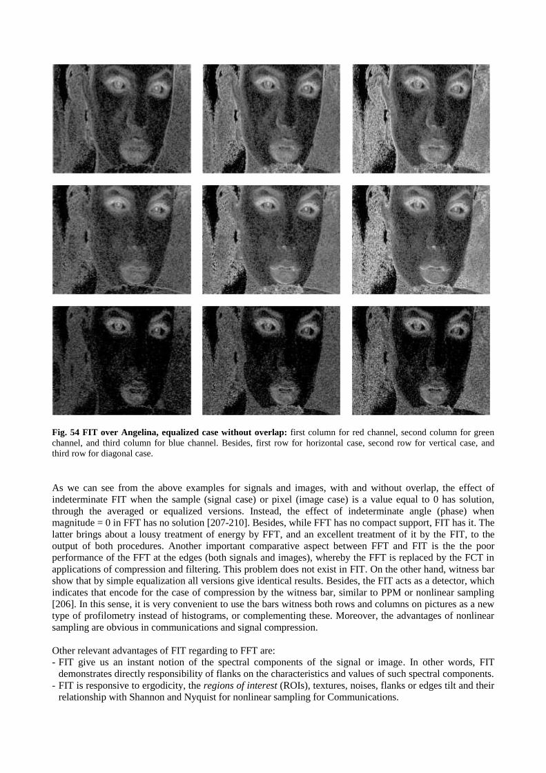
Fig. 54 FIT over Angelina, equalized case without overlap: first column for red channel, second column for green

channel, and third column for blue channel. Besides, first row for horizontal case, second row for vertical case, and

third row for diagonal case.

As we can see from the above examples for signals and images, with and without overlap, the effect of

indeterminate FIT when the sample (signal case) or pixel (image case) is a value equal to 0 has solution,

through the averaged or equalized versions. Instead, the effect of indeterminate angle (phase) when

magnitude = 0 in FFT has no solution [207-210]. Besides, while FFT has no compact support, FIT has it. The

latter brings about a lousy treatment of energy by FFT, and an excellent treatment of it by the FIT, to the

output of both procedures. Another important comparative aspect between FFT and FIT is the the poor

performance of the FFT at the edges (both signals and images), whereby the FFT is replaced by the FCT in

applications of compression and filtering. This problem does not exist in FIT. On the other hand, witness bar

show that by simple equalization all versions give identical results. Besides, the FIT acts as a detector, which

indicates that encode for the case of compression by the witness bar, similar to PPM or nonlinear sampling

[206]. In this sense, it is very convenient to use the bars witness both rows and columns on pictures as a new

type of profilometry instead of histograms, or complementing these. Moreover, the advantages of nonlinear

sampling are obvious in communications and signal compression.

Other relevant advantages of FIT regarding to FFT are:

- FIT give us an instant notion of the spectral components of the signal or image. In other words, FIT

demonstrates directly responsibility of flanks on the characteristics and values of such spectral components.

- FIT is responsive to ergodicity, the regions of interest (ROIs), textures, noises, flanks or edges tilt and their

relationship with Shannon and Nyquist for nonlinear sampling for Communications.

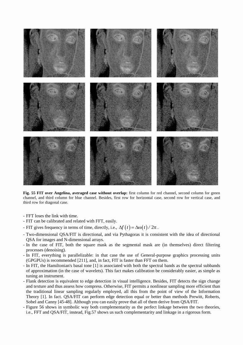
Fig. 55 FIT over Angelina, averaged case without overlap: first column for red channel, second column for green

channel, and third column for blue channel. Besides, first row for horizontal case, second row for vertical case, and

third row for diagonal case.

- FFT loses the link with time.

- FIT can be calibrated and related with FFT, easily.

- FIT gives frequency in terms of time, directly, i.e., 2f t t / .

- Two-dimensional QSA/FIT is directional, and via Pythagoras it is consistent with the idea of directional

QSA for images and N-dimensional arrays.

- In the case of FIT, both the square mask as the segmental mask are (in themselves) direct filtering

processes (denoising).

- In FIT, everything is parallelizable: in that case the use of General-purpose graphics processing units

(GPGPUs) is recommended [211], and, in fact, FIT is faster than FFT on them.

- In FIT, the Hamiltonian's basal tone [1] is associated with both the spectral bands as the spectral subbands

of approximation (in the case of wavelets). This fact makes calibration be considerably easier, as simple as

tuning an instrument.

- Flank detection is equivalent to edge detection in visual intelligence. Besides, FIT detects the sign change

and texture and thus assess how compress. Otherwise, FIT permits a nonlinear sampling more efficient than

the traditional linear sampling regularly employed, all this from the point of view of the Information

Theory [1]. In fact. QSA/FIT can perform edge detection equal or better than methods Prewitt, Roberts,

Sobel and Canny [45-48]. Although you can easily prove that all of them derive from QSA/FIT.

- Figure 56 shows in symbolic way both complementarity as the perfect linkage between the two theories,

i.e., FFT and QSA/FIT, instead, Fig.57 shows us such complementarity and linkage in a rigorous form.

Fig.56 Symbolic relationship between FIT and FFT (PSD).

Fig.57 Rigorous relationship between FIT and FFT (PSD).

Both graphs clearly show a quadrature between FFT and FIT via equalization.

FFT and FIT give information about the same physical element, i.e., the frequency, but in a very different

way, in fact, FIT is far superior and accurate (in its ambit) regarding FFT. Besides, unlike FFT, FIT has

compact support. However, both are complementary.

Thanks to these two tools (FFT and FIT) we can get the whole universe linked to spectral and temporal

analysis (simultaneously) of a signal, image or video. Therefore, we can locate (indirectly) to the FFT at the

exact time of the signal by its components. This fact implies a significant advance in the Fourier’s theory

after almost two and a half centuries.

On the other hand, the distribution of the witness bars is consistent with the possibility of locating a particle

by the wave function, or rather, the probability distribution that arises from this function.

Given the signal y = f (t), the witness bars arise as follows:

1. N equidistant lines are distributed along the ordinate axis

2. In those settings where these lines intercept the signal, we identify the projections on the axis of

abscissae. At these points we place the witness bars, which (if the signal is nonlinear) shall be

separated in a not equidistant way depending on the flanks of the signal at each point. This is a

nonlinear sampling itself.

Equations (166-168) for one dimensional case (signals) and (179, 195, 212-214) for two dimensional case

(images) represent a type of wavelets known as spectral wavelets, or simply, spectralets. In fact, it is the only

case inside wavelets, where high frequency sub-bands (or detail) represent spectral components (unlike

traditional wavelet). Such is the case that FIT is measured in Hertz. As we see in the next section, the

spectralets are also useful in the case of multislicing (image sequence processing [212], and medical images

[213], such as: Magnetic Resonance and Computer Tomography), multi [214-217] and hyperspectral

imagery [218-220], and video [201, 202, 221-226]. Besides, they serve to filtering, compression, edge

detection and superresolution. For example, for denoising and compression we can use the traditional

method of Dohono (thresholding/shrinkage) [125-127], and the smoothing of coefficients via median filter

[45-48], directional smoothing [162, 172], or enhanced directional smoothing [171] on detail subbands.

Additionally, spectralets are consistent with the procedure known as splitting of spectral subbands used in

the traditional wavelet (see Section 2.2), which continues recursively on approximation and detail subbands

(Li and Hi for signals; LLi and LHi, HLi, HHi for images; and LLLi and LLH i, LHL i, LHH i, HLL i, HLH i,

HHL i, HHH i for image sequence processing, being i the level of splitting). In fact, Haar is a particular case

of spectralets, see Eq(173) for one-dimensional case, and Eqs(227-229, 233-235) for two-dimensional case.

Complementary to this, in the next section, we will see a new concept inside wavelet theory called cosine

wavelets, or simply, coslets, which will be a key in all those applications like superresolution of biomedical

signals, still images for mobile, and video for video too.

Some final considerations:

- The transition from QSA to FIT represents the collapse of the wave function, i.e., from vector to scalar at

each moment.

- Hamiltonian is real, i.e., it isn’t hermitic for a confined single particle

- QSA/FIT is a time filter

- The frequency of a tone (sine) is proportional to its higher slope derivative. If it's a gate, will be infinite. In

the latter example, the density of the witness bars is infinite in the flank of the gate. This is very useful for a

better understanding of Sampling and Nyquist theorems.

- Like the FFT, the FIT will help in the development of new algorithms for signal, image and video

compression, replacing or complementing to FFT or DCT in new versions of, MP3 (audio [228]), JPEG

(images [227]) and, H.264 and VP9 (video [221-226]).

- Unlike FFT, FIT does not require decimation in time or frequency.

- For one-dimension FFT has a computational cost of O(N*log2(N)), and FIT of O(N).

- For two-dimensions FFT has a computational cost of O(N2*log2(N)2), and FIT of O(N2).

4 Simulations

4.1 Prolegomenous to simulations

In this section we will see only some possible applications of QSA/FIT, given that several of them we have

seen them in Section 3, e.g., spectral analysis. Besides, in addition, we also see some additional tools, which

will be very useful in this field.

4.1.1 Important tools

Coslets: without loss of generality, we present this new tool for two-dimensional case, however, it is possible

to make a generalization to one and three dimensions, in an easy and automatic way.

In here, we present a new multirresolution procedure based on DCT using this like a wavelet basis, See

Fig.58. For example, for an image I of size ROW-by-COL we have,

1) Choose image I(r,c) / r 1,ROW c 1,COL

2) J = DCT-2D(I) (236)

3) We obtain four subbands from 1 1

1 1

ll lhJ

hl hh

, with (237)

1

ROW COLll r,c / r 1, c 1,

2 2

,

1

ROW COLlh r,c / r 1, c 1,COL

2 2

,

1

ROW COLhl r,c / r 1,ROW c 1,

2 2

, and

1

ROW COLhh r,c / r 1,ROW c 1,COL

2 2

.

4) We apply iDCT-2D to each subband of J. Then, we obtain,

LL1 = iDCT-2D(ll1), with 1

ROW COLLL r,c / r 1, c 1,

2 2

, (238a)

LH1 = iDCT-2D(lh1), with 1

ROW COLLH r,c / r 1, c 1,COL

2 2

, (238b)

HL1 = iDCT-2D(hl1), with 1

ROW COLHL r,c / r 1,ROW c 1,

2 2

, and (238c)

HH1 = iDCT-2D(hh1), with 1

ROW COLHH r,c / r 1,ROW c 1,COL

2 2

. (238d)

From now on, the treatment is similar to the two-dimensional discrete wavelet transform, e.g., Haar [162-

170], see Section 2.2.2.

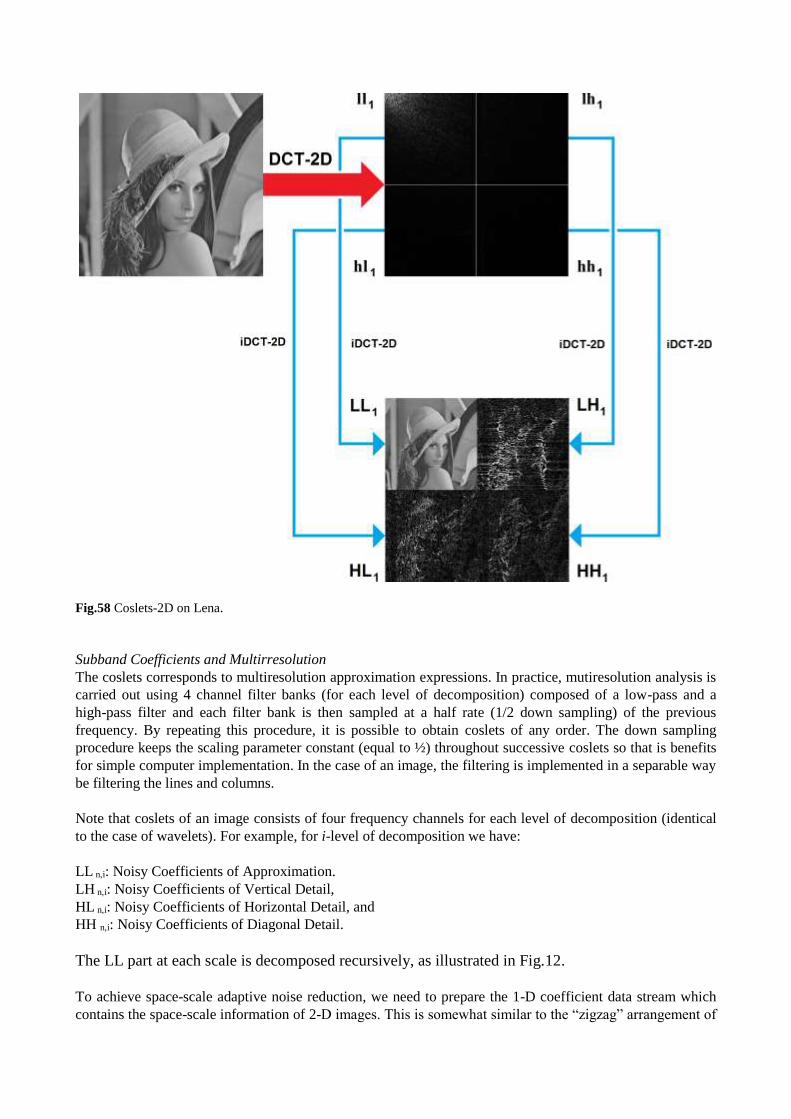
Fig.58 Coslets-2D on Lena.

Subband Coefficients and Multirresolution

The coslets corresponds to multiresolution approximation expressions. In practice, mutiresolution analysis is

carried out using 4 channel filter banks (for each level of decomposition) composed of a low-pass and a

high-pass filter and each filter bank is then sampled at a half rate (1/2 down sampling) of the previous

frequency. By repeating this procedure, it is possible to obtain coslets of any order. The down sampling

procedure keeps the scaling parameter constant (equal to ½) throughout successive coslets so that is benefits

for simple computer implementation. In the case of an image, the filtering is implemented in a separable way

be filtering the lines and columns.

Note that coslets of an image consists of four frequency channels for each level of decomposition (identical

to the case of wavelets). For example, for i-level of decomposition we have:

LL n,i: Noisy Coefficients of Approximation.

LH n,i: Noisy Coefficients of Vertical Detail,

HL n,i: Noisy Coefficients of Horizontal Detail, and

HH n,i: Noisy Coefficients of Diagonal Detail.

The LL part at each scale is decomposed recursively, as illustrated in Fig.12.

To achieve space-scale adaptive noise reduction, we need to prepare the 1-D coefficient data stream which

contains the space-scale information of 2-D images. This is somewhat similar to the “zigzag” arrangement of

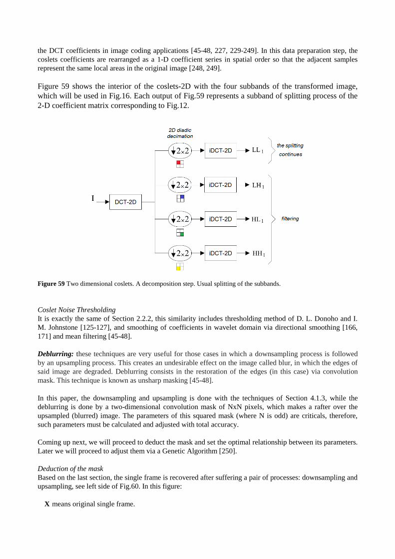
the DCT coefficients in image coding applications [45-48, 227, 229-249]. In this data preparation step, the

coslets coefficients are rearranged as a 1-D coefficient series in spatial order so that the adjacent samples

represent the same local areas in the original image [248, 249].

Figure 59 shows the interior of the coslets-2D with the four subbands of the transformed image,

which will be used in Fig.16. Each output of Fig.59 represents a subband of splitting process of the

2-D coefficient matrix corresponding to Fig.12.

Figure 59 Two dimensional coslets. A decomposition step. Usual splitting of the subbands.

Coslet Noise Thresholding

It is exactly the same of Section 2.2.2, this similarity includes thresholding method of D. L. Donoho and I.

M. Johnstone [125-127], and smoothing of coefficients in wavelet domain via directional smoothing [166,

171] and mean filtering [45-48].

Deblurring: these techniques are very useful for those cases in which a downsampling process is followed

by an upsampling process. This creates an undesirable effect on the image called blur, in which the edges of

said image are degraded. Deblurring consists in the restoration of the edges (in this case) via convolution

mask. This technique is known as unsharp masking [45-48].

In this paper, the downsampling and upsampling is done with the techniques of Section 4.1.3, while the

deblurring is done by a two-dimensional convolution mask of NxN pixels, which makes a rafter over the

upsampled (blurred) image. The parameters of this squared mask (where N is odd) are criticals, therefore,

such parameters must be calculated and adjusted with total accuracy.

Coming up next, we will proceed to deduct the mask and set the optimal relationship between its parameters.

Later we will proceed to adjust them via a Genetic Algorithm [250].

Deduction of the mask

Based on the last section, the single frame is recovered after suffering a pair of processes: downsampling and

upsampling, see left side of Fig.60. In this figure:

X means original single frame.

Y means recovered (blurred) single frame.

Mb means square mask of NxN pixels (where N is odd).

means downsampling.

means upsampling.

This mask is known as a blurred mask, smoothing operator or Point Spread Function (PSF) [251].

Figure 60 Downsampling/upsampling as a blurred mask.

In these processes ( and ), the single frame is affected by a space/time invariant blur, we which interpret

as the result of the action of a two-dimensional convolution between the original single frame and a mask

known in Digital Image Processing as a mask of mean filtering. The idea of mean filtering is simply to

replace each pixel value in an image with the mean (`average') value of its neighbors, including itself. This

has the effect of eliminating pixel values which are unrepresentative of their surroundings. Mean filtering is

usually thought of as a convolution filter. Like other convolutions it is based around a kernel, which

represents the shape and size of the neighborhood to be sampled when calculating the mean. Often a 3×3

square kernel is used, although larger kernels (e.g. 5×5 squares) can be used for more severe smoothing.

(Note that a small kernel can be applied more than once in order to produce a similar but not identical effect

as a single pass with a large kernel). In Fig.61, we consider the most general case, for N×N kernel, always

with odd N, where:

NN

1 (239)

Figure 61 N×N averaging kernel often used in mean filtering.

Computing the straightforward convolution of an image with this kernel carries out the mean filtering

process.

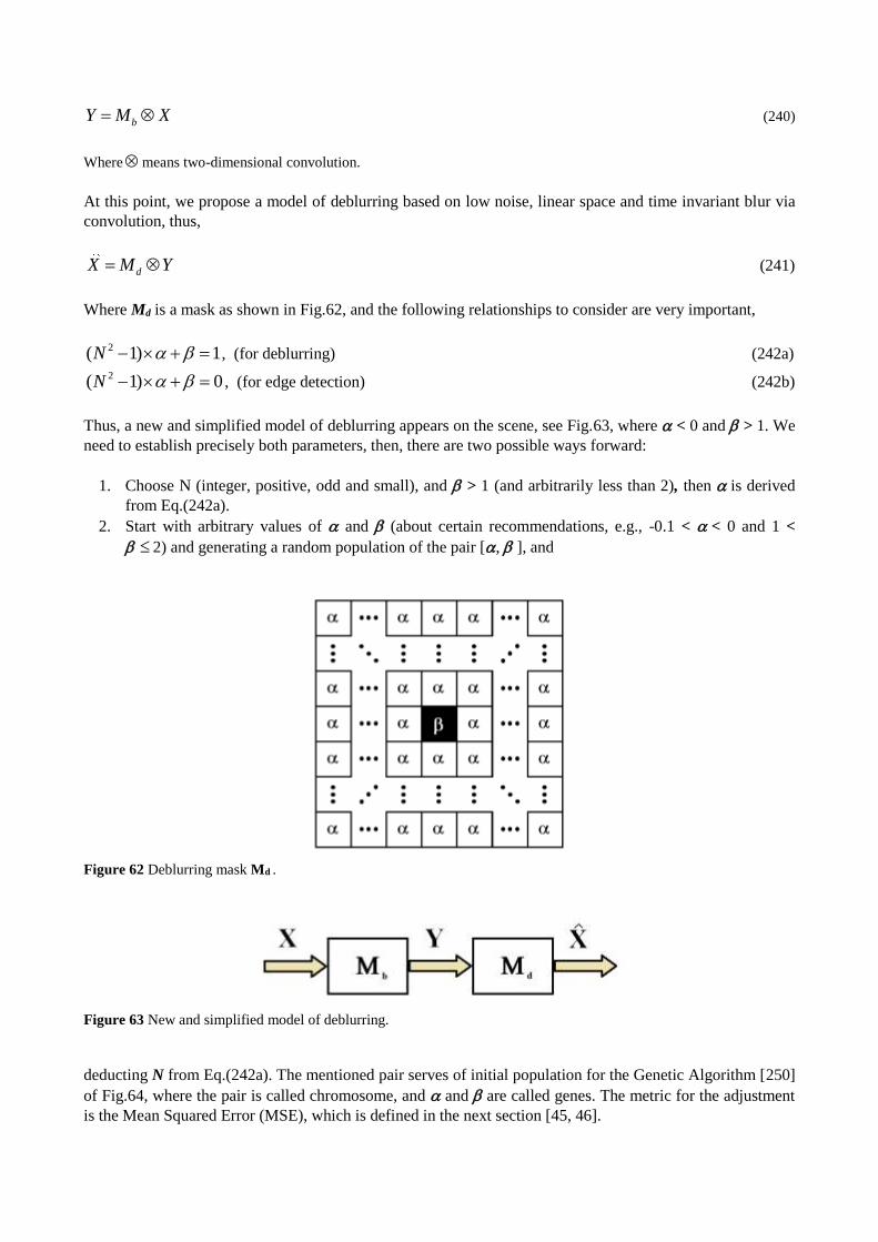
bY M X (240)

Wheremeans two-dimensional convolution.

At this point, we propose a model of deblurring based on low noise, linear space and time invariant blur via

convolution, thus,

dX M Y (241)

Where Md is a mask as shown in Fig.62, and the following relationships to consider are very important,

1)1( 2 N , (for deblurring) (242a)

0)1( 2 N , (for edge detection) (242b)

Thus, a new and simplified model of deblurring appears on the scene, see Fig.63, where < 0 and > 1. We

need to establish precisely both parameters, then, there are two possible ways forward:

1. Choose N (integer, positive, odd and small), and > 1 (and arbitrarily less than 2), then is derived

from Eq.(242a).

2. Start with arbitrary values of and (about certain recommendations, e.g., -0.1 < < 0 and 1 <

2) and generating a random population of the pair [, ], and

Figure 62 Deblurring mask Md .

Figure 63 New and simplified model of deblurring.

deducting N from Eq.(242a). The mentioned pair serves of initial population for the Genetic Algorithm [250]

of Fig.64, where the pair is called chromosome, and and are called genes. The metric for the adjustment

is the Mean Squared Error (MSE), which is defined in the next section [45, 46].

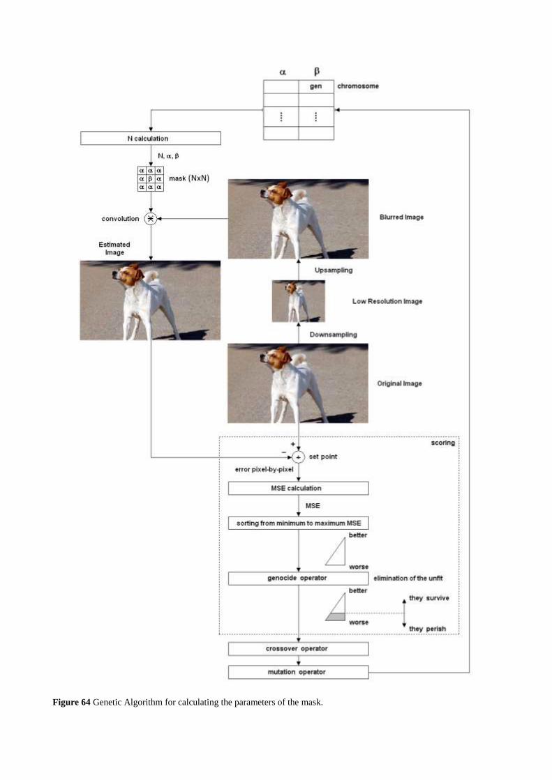
Figure 64 Genetic Algorithm for calculating the parameters of the mask.

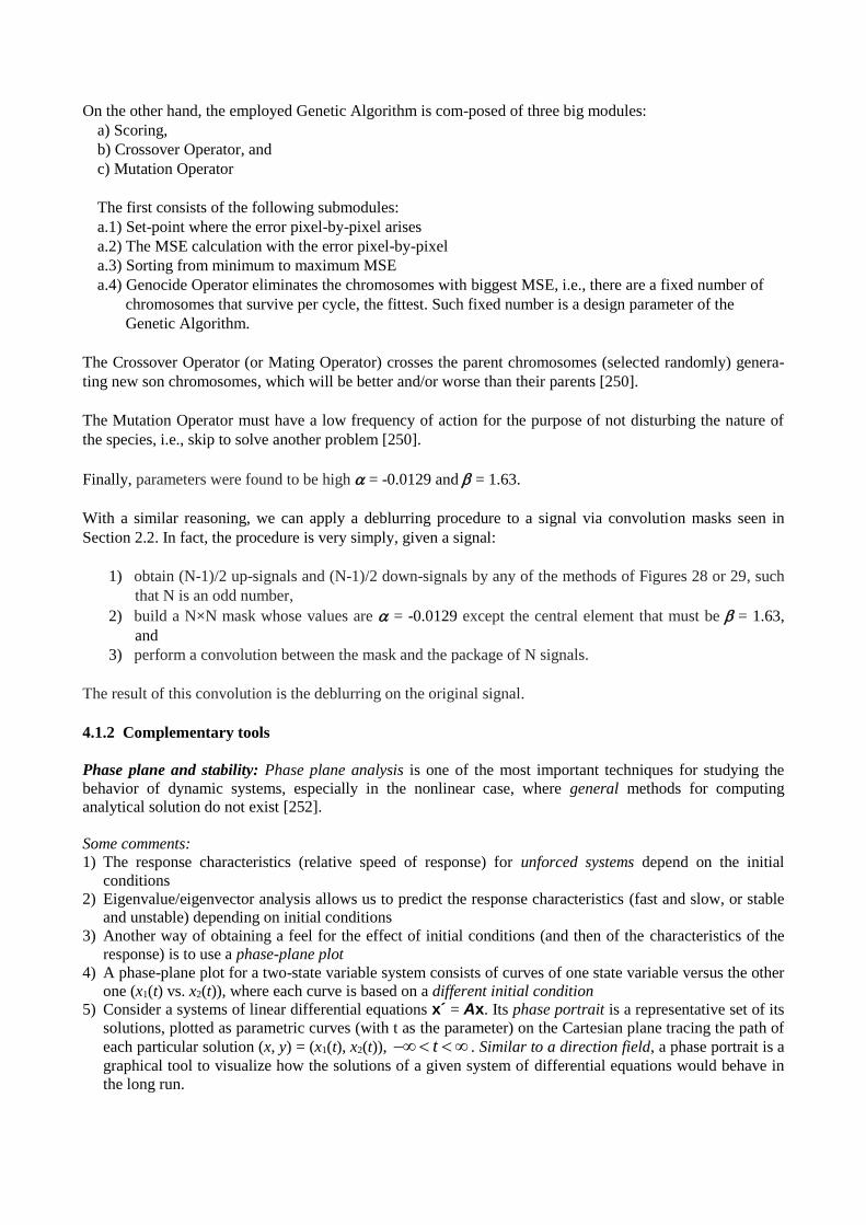
On the other hand, the employed Genetic Algorithm is com-posed of three big modules:

a) Scoring,

b) Crossover Operator, and

c) Mutation Operator

The first consists of the following submodules:

a.1) Set-point where the error pixel-by-pixel arises

a.2) The MSE calculation with the error pixel-by-pixel

a.3) Sorting from minimum to maximum MSE

a.4) Genocide Operator eliminates the chromosomes with biggest MSE, i.e., there are a fixed number of

chromosomes that survive per cycle, the fittest. Such fixed number is a design parameter of the

Genetic Algorithm.

The Crossover Operator (or Mating Operator) crosses the parent chromosomes (selected randomly) genera-

ting new son chromosomes, which will be better and/or worse than their parents [250].

The Mutation Operator must have a low frequency of action for the purpose of not disturbing the nature of

the species, i.e., skip to solve another problem [250].

Finally, parameters were found to be high = -0.0129 and = 1.63.

With a similar reasoning, we can apply a deblurring procedure to a signal via convolution masks seen in

Section 2.2. In fact, the procedure is very simply, given a signal:

1) obtain (N-1)/2 up-signals and (N-1)/2 down-signals by any of the methods of Figures 28 or 29, such

that N is an odd number,

2) build a N×N mask whose values are = -0.0129 except the central element that must be = 1.63,

and

3) perform a convolution between the mask and the package of N signals.

The result of this convolution is the deblurring on the original signal.

4.1.2 Complementary tools

Phase plane and stability: Phase plane analysis is one of the most important techniques for studying the

behavior of dynamic systems, especially in the nonlinear case, where general methods for computing

analytical solution do not exist [252].

Some comments:

1) The response characteristics (relative speed of response) for unforced systems depend on the initial

conditions

2) Eigenvalue/eigenvector analysis allows us to predict the response characteristics (fast and slow, or stable

and unstable) depending on initial conditions

3) Another way of obtaining a feel for the effect of initial conditions (and then of the characteristics of the

response) is to use a phase-plane plot

4) A phase-plane plot for a two-state variable system consists of curves of one state variable versus the other

one (x1(t) vs. x2(t)), where each curve is based on a different initial condition

5) Consider a systems of linear differential equations x´ = Ax. Its phase portrait is a representative set of its

solutions, plotted as parametric curves (with t as the parameter) on the Cartesian plane tracing the path of

each particular solution (x, y) = (x1(t), x2(t)), t . Similar to a direction field, a phase portrait is a

graphical tool to visualize how the solutions of a given system of differential equations would behave in

the long run.

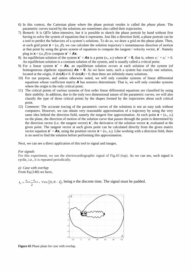
6) In this context, the Cartesian plane where the phase portrait resides is called the phase plane. The

parametric curves traced by the solutions are sometimes also called their trajectories.

7) Remark: It is QITe labor-intensive, but it is possible to sketch the phase portrait by hand without first

having to solve the system of equations that it represents. Just like a direction field, a phase portrait can be

a tool to predict the behaviors of a system’s solutions. To do so, we draw a grid on the phase plane. Then,

at each grid point x = (, ), we can calculate the solution trajectory’s instantaneous direction of motion

at that point by using the given system of equations to compute the tangent / velocity vector, x´. Namely

plug in x = (, ) to compute x´ = Ax.

8) An equilibrium solution of the system x´ = Ax is a point (x1, x2) where x´ = 0, that is, where x1´ = x2´ = 0.

An equilibrium solution is a constant solution of the system, and is usually called a critical point.

9) For a linear system x´ = Ax, an equilibrium solution occurs at each solution of the system (of

homogeneous algebraic equations) Ax = 0. As we have seen, such a system has exactly one solution,

located at the origin, if det(A) 0. If det(A) = 0, then there are infinitely many solutions.

10) For our purpose, and unless otherwise noted, we will only consider systems of linear differential

equations whose coefficient matrix A has nonzero determinant. That is, we will only consider systems

where the origin is the only critical point.

11) The critical points of various systems of first order linear differential equations are classified by using

their stability. In addition, due to the truly two dimensional nature of the parametric curves, we will also

classify the type of those critical points by the shapes formed by the trajectories about each critical

point.

12) Comment: The accurate tracing of the parametric curves of the solutions is not an easy task without

computers. However, we can obtain very reasonable approximation of a trajectory by using the very

same idea behind the direction field, namely the tangent line approximation. At each point x = (x1, x2)

on the plane, the direction of motion of the solution curve that passes through the point is determined by

the direction vector (i.e. the tangent vector) x´, the derivative of the solution vector x, evaluated at the

given point. The tangent vector at each given point can be calculated directly from the given matrix

vector equation x´ = Ax, using the position vector x = (x1, x2). Like working with a direction field, there

is no need to find the solution before performing this approximation.

Next, we can see a direct application of this tool to signal and images.

For signals

For this experiment, we use the electrocardiographic signal of Fig.43 (top). As we can see, such signal is

cyclic, i.e., it is repeated periodically.

a) Case with overlap

From Eq.(140) we have,

1 1

2

n nn

s ss , 0 1n ,N , being n the discrete time. The signal must be padded.

Figure 65 Phase plane for case with overlap.

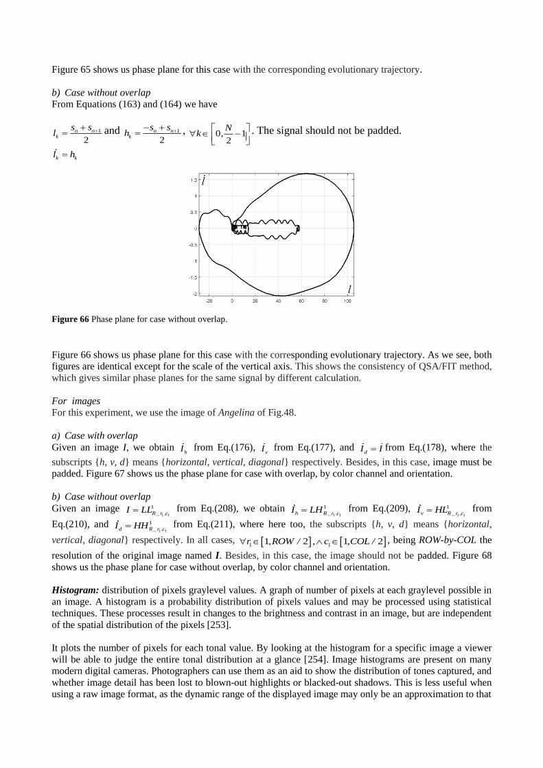
Figure 65 shows us phase plane for this case with the corresponding evolutionary trajectory.

b) Case without overlap

From Equations (163) and (164) we have

1

2

n nk

s sl and 1

2

n nk

s sh , 0 1

2

Nk ,

. The signal should not be padded.

k kl h

Figure 66 Phase plane for case without overlap.

Figure 66 shows us phase plane for this case with the corresponding evolutionary trajectory. As we see, both

figures are identical except for the scale of the vertical axis. This shows the consistency of QSA/FIT method,

which gives similar phase planes for the same signal by different calculation.

For images

For this experiment, we use the image of Angelina of Fig.48.

a) Case with overlap

Given an image I, we obtain hI from Eq.(176),

vI from Eq.(177), and dI I from Eq.(178), where the

subscripts {h, v, d} means {horizontal, vertical, diagonal} respectively. Besides, in this case, image must be

padded. Figure 67 shows us the phase plane for case with overlap, by color channel and orientation.

b) Case without overlap

Given an image 1 1

1

R _ r ,cI LL from Eq.(208), we obtain 1 1

1

h R _r ,cI LH from Eq.(209), 1 1

1

v R _ r ,cI HL from

Eq.(210), and 1 1

1

d R _r ,cI HH from Eq.(211), where here too, the subscripts {h, v, d} means {horizontal,

vertical, diagonal} respectively. In all cases, 1 11 2 1 2r ,ROW / , c ,COL / , being ROW-by-COL the

resolution of the original image named I. Besides, in this case, the image should not be padded. Figure 68

shows us the phase plane for case without overlap, by color channel and orientation.

Histogram: distribution of pixels graylevel values. A graph of number of pixels at each graylevel possible in

an image. A histogram is a probability distribution of pixels values and may be processed using statistical

techniques. These processes result in changes to the brightness and contrast in an image, but are independent

of the spatial distribution of the pixels [253].

It plots the number of pixels for each tonal value. By looking at the histogram for a specific image a viewer

will be able to judge the entire tonal distribution at a glance [254]. Image histograms are present on many

modern digital cameras. Photographers can use them as an aid to show the distribution of tones captured, and

whether image detail has been lost to blown-out highlights or blacked-out shadows. This is less useful when

using a raw image format, as the dynamic range of the displayed image may only be an approximation to that

red green blue

h

v

d

Figure 67 Phase plane for case with overlap, by color channel and orientation.

in the raw file. The horizontal axis of the graph represents the tonal variations, while the vertical axis

represents the number of pixels in that particular tone. The left side of the horizontal axis represents the black

and dark areas, the middle represents medium grey and the right hand side represents light and pure white

areas. The vertical axis represents the size of the area that is captured in each one of these zones. Thus, the

histogram for a very dark image will have the majority of its data points on the left side and center of the

graph. Conversely, the histogram for a very bright image with few dark areas and/or shadows will have most

of its data points on the right side and center of the graph. Finally, Fig.69 shows an image of Angelina and its

histogram.

As Prof. Emmanuel Agu says [255]: histograms is an important tool, because

• They help detect image acquisition issues

• Problems with image can be identified on histogram, such as:

Over and under exposure

Brightness

Contrast

Dynamic Range

• Point operations can be used to alter histogram, e.g.:

Addition

Multiplication

Exponential and Logarithmic

Intensity windowing (contrast modification)

With regard to the interpretation of the histograms, Logarithmic scale makes low values more visible. This

allows a marked difference between darkest and lightest. See Fig.70.

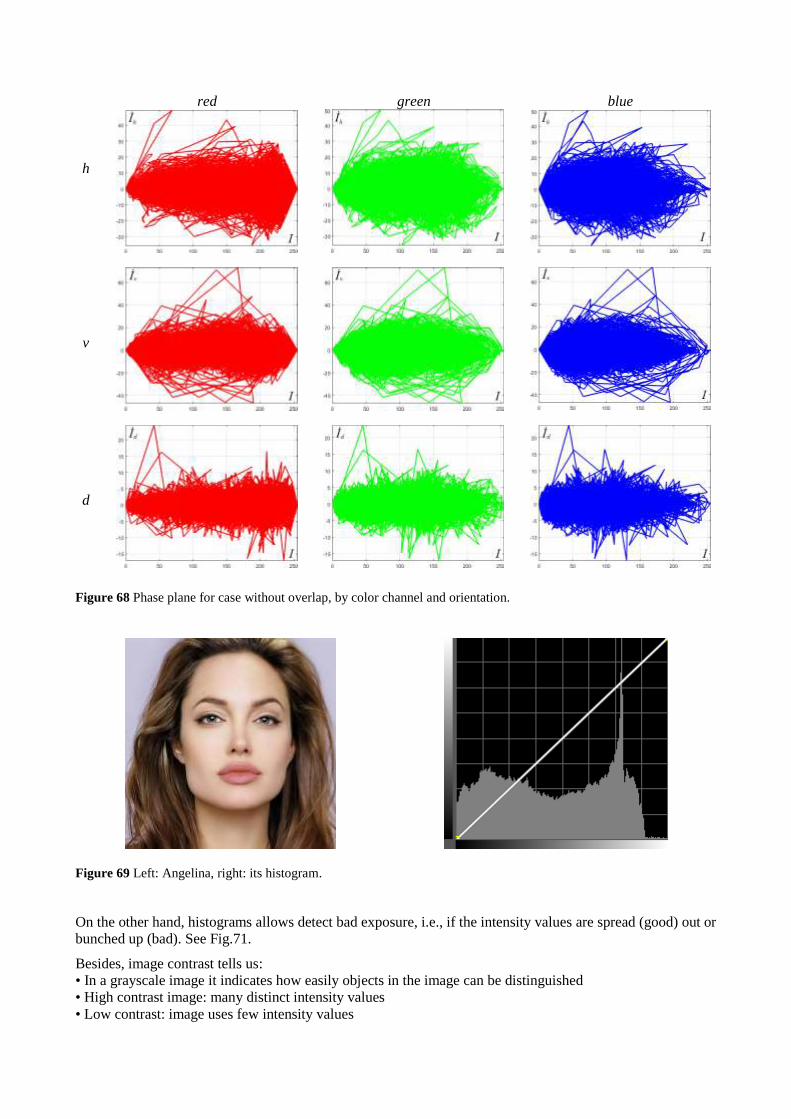
red green blue

h

v

d

Figure 68 Phase plane for case without overlap, by color channel and orientation.

Figure 69 Left: Angelina, right: its histogram.

On the other hand, histograms allows detect bad exposure, i.e., if the intensity values are spread (good) out or

bunched up (bad). See Fig.71.

Besides, image contrast tells us:

• In a grayscale image it indicates how easily objects in the image can be distinguished

• High contrast image: many distinct intensity values

• Low contrast: image uses few intensity values

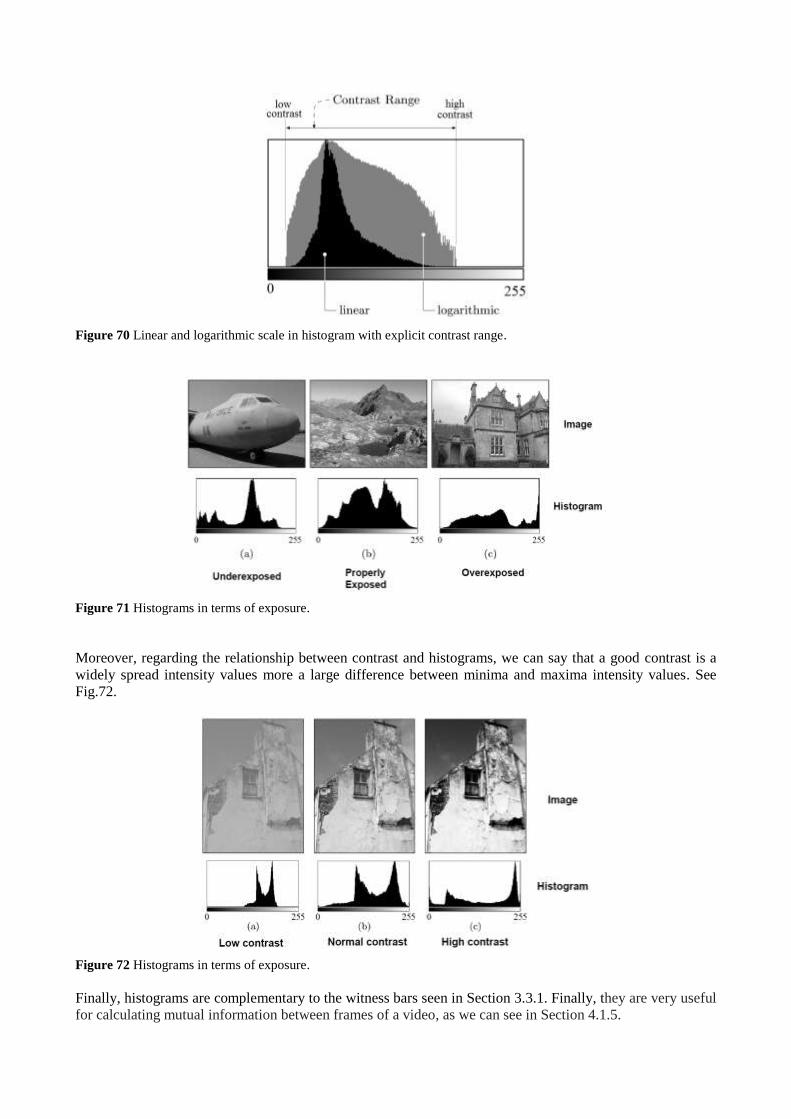
Figure 70 Linear and logarithmic scale in histogram with explicit contrast range.

Figure 71 Histograms in terms of exposure.

Moreover, regarding the relationship between contrast and histograms, we can say that a good contrast is a

widely spread intensity values more a large difference between minima and maxima intensity values. See

Fig.72.

Figure 72 Histograms in terms of exposure.

Finally, histograms are complementary to the witness bars seen in Section 3.3.1. Finally, they are very useful

for calculating mutual information between frames of a video, as we can see in Section 4.1.5.

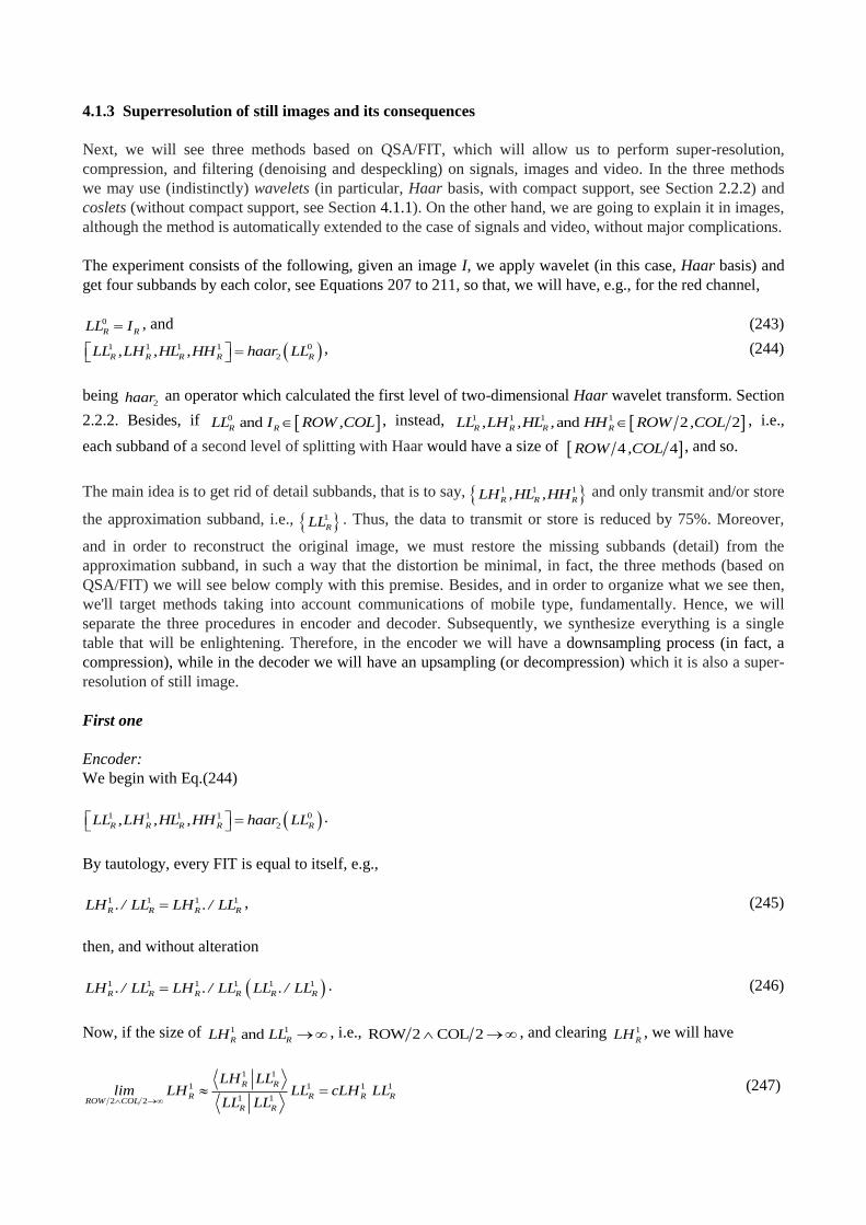
4.1.3 Superresolution of still images and its consequences

Next, we will see three methods based on QSA/FIT, which will allow us to perform super-resolution,

compression, and filtering (denoising and despeckling) on signals, images and video. In the three methods

we may use (indistinctly) wavelets (in particular, Haar basis, with compact support, see Section 2.2.2) and

coslets (without compact support, see Section 4.1.1). On the other hand, we are going to explain it in images,

although the method is automatically extended to the case of signals and video, without major complications.

The experiment consists of the following, given an image I, we apply wavelet (in this case, Haar basis) and

get four subbands by each color, see Equations 207 to 211, so that, we will have, e.g., for the red channel,

0

R RLL I , and (243)

1 1 1 1 0

2R R R R RLL ,LH ,HL ,HH haar LL , (244)

being 2haar an operator which calculated the first level of two-dimensional Haar wavelet transform. Section

2.2.2. Besides, if 0 andR RLL I ROW ,COL , instead, 1 1 1 1and 2 2R R R RLL ,LH ,HL , HH ROW ,COL , i.e.,

each subband of a second level of splitting with Haar would have a size of 4 4ROW ,COL , and so.

The main idea is to get rid of detail subbands, that is to say, 1 1 1

R R RLH ,HL ,HH and only transmit and/or store

the approximation subband, i.e., 1

RLL . Thus, the data to transmit or store is reduced by 75%. Moreover,

and in order to reconstruct the original image, we must restore the missing subbands (detail) from the

approximation subband, in such a way that the distortion be minimal, in fact, the three methods (based on

QSA/FIT) we will see below comply with this premise. Besides, and in order to organize what we see then,

we'll target methods taking into account communications of mobile type, fundamentally. Hence, we will

separate the three procedures in encoder and decoder. Subsequently, we synthesize everything is a single

table that will be enlightening. Therefore, in the encoder we will have a downsampling process (in fact, a

compression), while in the decoder we will have an upsampling (or decompression) which it is also a super-

resolution of still image.

First one

Encoder:

We begin with Eq.(244)

1 1 1 1 0

2R R R R RLL ,LH ,HL ,HH haar LL .

By tautology, every FIT is equal to itself, e.g.,

1 1 1 1

R R R RLH . / LL LH . / LL , (245)

then, and without alteration

1 1 1 1 1 1

R R R R R RLH . / LL LH . / LL LL . / LL . (246)

Now, if the size of 1 1andR RLH LL , i.e., ROW 2 COL 2 , and clearing 1

RLH , we will have

1 1

1 1 1 1

1 12 2

R R

R R R RROW COL

R R

LH LLlim LH LL cLH LL

LL LL (247)

where

1 1

1

1 1

R R

R

R R

LH LLcLH

LL LL (248)

Identical case for 1 1andR RHL HH .

Finally, we eliminate to 1 1 1

R R RLH ,HL ,HH , and therefore, we transmit 1 1 1 1

R R R RLL ,cLH ,cHL ,cHH , being

1 1 1

R R RcLH ,cHL ,cHH simple scalars.

Equation (247) is equivalent to say mutual information between 1

RLH and 1 1

R RcLH LL is the maximum

possible for a technique that touch resolution. See Section 4.1.5.

Decoder:

From 1 1 1 1

R R R RLL ,cLH ,cHL ,cHH we rebuild 1 1 1

R R RLH ,HL ,HH , that is to say

1 1 1

R R RLH cLH LL (249a)

1 1 1

R R RHL cHL LL (249b)

1 1 1

R R RHH cHH LL . (249c)

Then, we apply

0 1 1 1 1

2R R R R RLL ihaar LL ,LH ,HL ,HH , (250)

where 2ihaar is an operator, which calculated the first level of inverse two-dimensional Haar wavelet trans-

form. Identical procedure for green and blue channels. Finally,

0

R RI LL (251)

If: a) the original image is small, or b) we use several levels of downsampling/upsampling, or c) the original

image comes from a previous filtering process, then, we need the deblurring technique of Section 4.1.1 for a

reconstruction of the edges and texture.

Second one

Encoder:

We begin with Eq.(244)

1 1 1 1 0

2R R R R RLL ,LH ,HL ,HH haar LL .

Then, we eliminate to 1 1 1

R R RLH ,HL ,HH , and we transmit only 1

RLL . This method is known in literature as

Rule of Three (Ro3), see [257].

Decoder:

First, we define something called replicated element of subband (RES), which is repeated 4 times the value

of each element of a matrix forming a macroelement. We can see this in a very simple example in Eq,(252).

In such equation, each element of the matrix is repeated in square shaped.

a a b b

a b a a b b

c d c c d d

c c d d

(252)

Then and always for red channel (as example), we apply,

2 2 2 2 1

2R R R R RLL ,LH ,HL ,HH haar LL . (253)

Now, we use operator res2(•) to each subband of second level of haar2 splitting,

2 2

2R _res RLL res LL , (254a)

2 2

2R _res RLH res LH , (254b)

2 2

2R _res RHL res HL , and (254c)

2 2

2R _res RHH res HH . (254d)

Therefore, if we make

1 1 2 2

2 2R R R_res R_res

ROW COLlim LH . / LL LH . / LL

(255)

where superscript 2 means second level of splitting thanks to haar2 . This means that FITs of consistent

levels of splitting (n and n+1) tend to the same value as the dimension of the matrices tends to infinity. This

also means that the mutual information between 1 2

R R _resLL and LL and 1 2

R R_resLH and LH is maximized for the

same circumstances. Thus,

1 1 2 2 2 2

R R R_res R_res R_res R_resLH . / LL LH . / LL LL . / LL (256)

Now, if the size of 1 1 2 2, , andR R R_res R_resLH LL , LH LL , i.e., ROW 2 COL 2 , and clearing 1

RLH ,

we will have

2 2

1 1

2 22 2

R _ res R _ res

R RROW COL

R _ res R _ res

LH LLlim LH LL

LL LL (257)

Therefore,

2 2

1 1

2 2

R _ res R _ res

R R

R _ res R _ res

LH LLLH LL

LL LL

(258a)

2 2

1 1

2 2

R _ res R _ res

R R

R _ res R _ res

HL LLHL LL

LL LL

(258b)

2 2

1 1

2 2

R _ res R _ res

R R

R _ res R _ res

HH LLHH LL

LL LL

(258c)

Another version element-by-element presented in [257] is

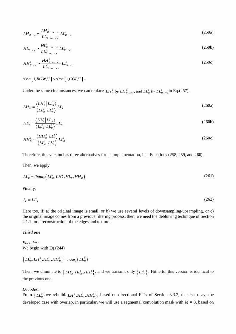
2

1 1

2

R _ res _ r ,c

R _ r ,c R _ r ,c

R _ res _ r ,c

LHLH LL

LL (259a)

2

1 1

2

R _ res _ r ,c

R _ r ,c R _ r ,c

R _ res _ r ,c

HLHL LL

LL (259b)

2

1 1

2

R _ res _ r ,c

R _ r ,c R _ r ,c

R _ res _ r ,c

HHHH LL

LL (259c)

1 2 1 2r ,ROW c ,COL .

Under the same circumstances, we can replace 2 2 2 2, andR R_res R R_resLH by LH LL by LL in Eq.(257),

2 2

1 1

2 2

R R

R R

R R

LH LLLH LL

LL LL

(260a)

2 2

1 1

2 2

R R

R R

R R

HL LLHL LL

LL LL

(260b)

2 2

1 1

2 2

R R

R R

R R

HH LLHH LL

LL LL

(260c)

Therefore, this version has three alternatives for its implementation, i.e., Equations (258, 259, and 260).

Then, we apply

0 1 1 1 1

2R R R R RLL ihaar LL ,LH ,HL ,HH , (261)

Finally,

0

R RI LL (262)

Here too, if: a) the original image is small, or b) we use several levels of downsampling/upsampling, or c)

the original image comes from a previous filtering process, then, we need the deblurring technique of Section

4.1.1 for a reconstruction of the edges and texture.

Third one

Encoder:

We begin with Eq.(244)

1 1 1 1 0

2R R R R RLL ,LH ,HL ,HH haar LL .

Then, we eliminate to 1 1 1

R R RLH ,HL ,HH , and we transmit only 1

RLL . Hitherto, this version is identical to

the previous one.

Decoder:

From 1

RLL we rebuild 1 1 1

R R RLH ,HL ,HH , based on directional FITs of Section 3.3.2, that is to say, the

developed case with overlap, in particular, we will use a segmental convolution mask with M = 3, based on

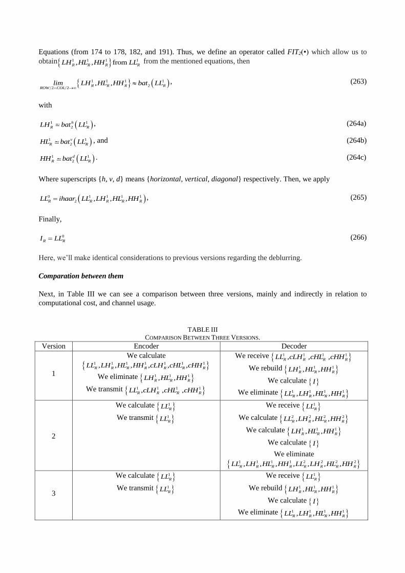
Equations (from 174 to 178, 182, and 191). Thus, we define an operator called FIT2(•) which allow us to

obtain 1 1 1 1fromR R R RLH ,HL ,HH LL from the mentioned equations, then

1 1 1 1

22 2

R R R RROW COL

lim LH ,HL ,HH bat LL

, (263)

with

1 1

2

h

R RLH bat LL , (264a)

1 1

2

v

R RHL bat LL , and (264b)

1 1

2

d

R RHH bat LL . (264c)

Where superscripts {h, v, d} means {horizontal, vertical, diagonal} respectively. Then, we apply

0 1 1 1 1

2R R R R RLL ihaar LL ,LH ,HL ,HH , (265)

Finally,

0

R RI LL (266)

Here, we’ll make identical considerations to previous versions regarding the deblurring.

Comparation between them

Next, in Table III we can see a comparison between three versions, mainly and indirectly in relation to

computational cost, and channel usage.

TABLE III

COMPARISON BETWEEN THREE VERSIONS.

Version Encoder Decoder

1

We calculate

1 1 1 1 1 1 1

R R R R R R RLL ,LH ,HL ,HH ,cLH ,cHL ,cHH

We eliminate 1 1 1

R R RLH ,HL ,HH

We transmit 1 1 1 1

R R R RLL ,cLH ,cHL ,cHH

We receive 1 1 1 1

R R R RLL ,cLH ,cHL ,cHH

We rebuild 1 1 1

R R RLH ,HL ,HH

We calculate I

We eliminate 1 1 1 1

R R R RLL ,LH ,HL ,HH

2

We calculate 1

RLL

We transmit 1

RLL

We receive 1

RLL

We calculate 2 2 2 2

R R R RLL ,LH ,HL ,HH

We calculate 1 1 1

R R RLH ,HL ,HH

We calculate I

We eliminate

1 1 1 1 2 2 2 2

R R R R R R R RLL ,LH ,HL ,HH ,LL ,LH ,HL ,HH

3

We calculate 1

RLL

We transmit 1

RLL

We receive 1

RLL

We rebuild 1 1 1

R R RLH ,HL ,HH

We calculate I

We eliminate 1 1 1 1

R R R RLL ,LH ,HL ,HH

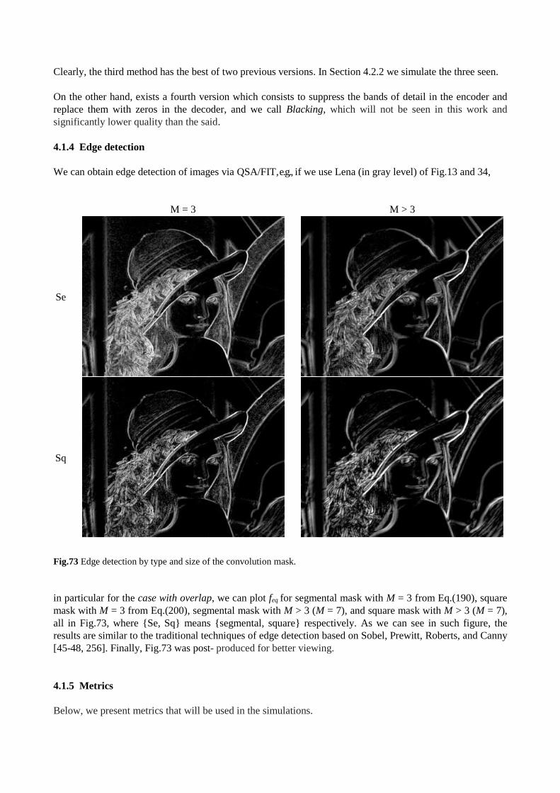
Clearly, the third method has the best of two previous versions. In Section 4.2.2 we simulate the three seen.

On the other hand, exists a fourth version which consists to suppress the bands of detail in the encoder and

replace them with zeros in the decoder, and we call Blacking, which will not be seen in this work and

significantly lower quality than the said.

4.1.4 Edge detection

We can obtain edge detection of images via QSA/FIT, e.g., if we use Lena (in gray level) of Fig.13 and 34,

M = 3 M > 3

Se

Sq

Fig.73 Edge detection by type and size of the convolution mask.

in particular for the case with overlap, we can plot feq for segmental mask with M = 3 from Eq.(190), square

mask with M = 3 from Eq.(200), segmental mask with M > 3 (M = 7), and square mask with M > 3 (M = 7),

all in Fig.73, where {Se, Sq} means {segmental, square} respectively. As we can see in such figure, the

results are similar to the traditional techniques of edge detection based on Sobel, Prewitt, Roberts, and Canny

[45-48, 256]. Finally, Fig.73 was post- produced for better viewing.

4.1.5 Metrics

Below, we present metrics that will be used in the simulations.

Data Compression Ratio (CR)

Data compression ratio, also known as compression power, is a computer-science term used to quantify the

reduction in data-representation size produced by a data compression algorithm. The data compression ratio

is analogous to the physical compression ratio used to measure physical compression of substances, and is

defined in the same way, as the ratio between the uncompressed size and the compressed size [45]:

SizeCompressed

SizeedUncompressCR (267)

Thus a representation that compresses a 10MB file to 2MB has a compression ratio of 10/2 = 5, often notated

as an explicit ratio, 5:1 (read "five to one"), or as an implicit ratio, 5X. Note that this formulation applies

equally for compression, where the uncompressed size is that of the original; and for decompression, where

the uncompressed size is that of the reproduction.

Percent Space Savings (PSS)

Sometimes the space savings is given instead, which is defined as the reduction in size relative to the

uncompressed size:

%100*1

1

CRPSS (268)

Thus a representation that compresses 10MB file to 2MB would yield a space savings of 1-2/10 = 0.8, often

notated as a percentage, 80%.

Peak Signal-To-Noise Ratio (PSNR)

The phrase peak signal-to-noise ratio, often abbreviated PSNR, is an engineering term for the ratio between

the maximum possible power of a signal and the power of corrupting noise that affects the fidelity of its

representation. Because many signals have a very wide dynamic range, PSNR is usually expressed in terms

of the logarithmic decibel scale.

The PSNR is most commonly used as a measure of quality of reconstruction in image compression etc [45].

It is most easily defined via the mean squared error (MSE) which for two NR×NC (rows-by-columns)

monochrome images I and Id , where the second one of the images is considered a decompressed/denoised

approximation of the other is defined as:

1 1

2

0 0

( , ) ( , )1

d

NR NC

nr ncNRxNCI nr nc I nr ncMSE

(269)

The PSNR is defined as [258]:

2

10 1010 log 20 logI I

MAX MAXPSNR

MSE MSE (270)

Here, MAXi is the maximum pixel value of the image. When the pixels are represented using 8 bits per

sample, this is 255. More generally, when samples are represented using linear pulse code modulation

(PCM) with B bits per sample, maximum possible value of MAXi is 2B-1.

For color images with three red-green-blue (RGB) values per pixel, the definition of PSNR is the same

except the MSE is the sum over all squared value differences divided by image size and by three [45]. A

similar situation occurs with the mean absolute error (MAE), which is discussed below.

Typical values for the PSNR in lossy image and video compression are between 30 and 50 dB, where higher

is better.

Finally, a conspicuous metric for these cases is the mean absolute error, which is a quantity used to measure

how close forecasts or predictions are to the eventual outcomes. The mean absolute error (MAE) is given by

1 1

0 0

( , ) ( , )1

d

NR NC

nr ncNRxNCI nr nc I nr ncMAE

(271)

which for two NR×NC (rows-by-columns) monochrome images I and Id , where the second one of the

images is considered a decompressed/denoised approximation of the other of the first one.

In the case of signals, MSE and MAE will be

1

2

0

( ) ( )1

d

N

nNS n S nMSE

(272)

0

( ) ( )1

d

N

nNS n S nMAE

(273)

while PSNR be

2

10 1010 log 20 logS S

MAX MAXPSNR

MSE MSE (274)

It’s easy to generalize {MAE, MSE, and PSNR} for images (2D) and video (3D).

Mutual Information between two matrices

Here, we are going to calculate the Mutual Information between two images, frames or matrices thanks to

marginal entropies and the joint entropy [259]. Therefore, Mutual information can be expressed as

, ,X Y X H Y H X YI H , (275)

where I(X;Y) is the mutual information between the two images, H(X) is the entropy of image X, H(Y) is the

entropy of image Y, and H(X,Y) is the joint entropy between images.

Entropy of an image

If X is the image, we begin with the normalization of X, i.e.,

1 1

, 1, 1,

( , )ROW COL

r c

XX r ROW c COL

X r c

, (276)

such that,

1 1

( , ) 1ROW COL

r c

X r c

, (277)

Thus,

2

1 1

( , ) log ( , )ROW COL

r c

H X X r c X r c

, (278)

Mutual Information between two images, frames or matrices

However, it is more practical to calculate the entropies (including the joint entropy, and hence the Mutual

Information) based on histograms as seen in Section 4.1.2. To this end, we recommend the MATLAB code

[49] developed by Jose Delpiano [260, 261].

4.2 Simulations properly speaking

For all experiments, we are going to use metrics of the last section. Besides, the employed signal will be that

of Fig.43, i.e., electrocardiographic (ECG) signal of 80 pulses per second, and 1024 samples per second,

while, for the image case, we will use to Angelina of Fig.48, with 1920-by-1080 pixels, and 24 bpp.

Finally, we only simulate those techniques that we consider conspicuous in order to test the strength of

QSA/FIT, or those that we have not simulated in the previous sections.

4.2.1 Denoising (and despeckling)

The general schema of the denoising procedure can be seen in Fig.74, where the signal (in fact, signal or

image) is corrupted by additive noise (or multiplicative noise of Gamma distribution known like speckle [50,

162-171, 199]). After the filter, we compare denoised and original image with a set of metrics like defined in

the last section, in order to test the filtering (denoising for additive noise and despeckling for multiplicative

noise or speckle) performance.

Fig.74 Filtering: denoising/despeckling.

Signals

In all cases, the signal is injected with a 5% of white noise with Gaussian distribution and zero mean value.

On the other hand, Table IV shows us denoising techniques vs metrics, where acronyms means:

SG: Savitzky-Golay

MF: Mean filter. In all cases M = 3, i.e., it is a square mask of 3x3.

DS: Directional Smoothing. In all cases M = 3, i.e., it is a square mask of 3x3.

ST: Soft-thresholding

HT: Hard-thresholding

SR-i: Super-resolution, version i

Clearly, Coslet is better than Haar basis in all applications. Moreover, although Savitzky-Golay has better

metric results, it is very slow regarding to the rest of techniques. Besides, Savitzky-Golay is used at its best

version, while the other at its worst version.

Figure 75 shows us corresponding simulations with noisy signal in red and denoised signal in blue. Clearly it

improved in all cases.

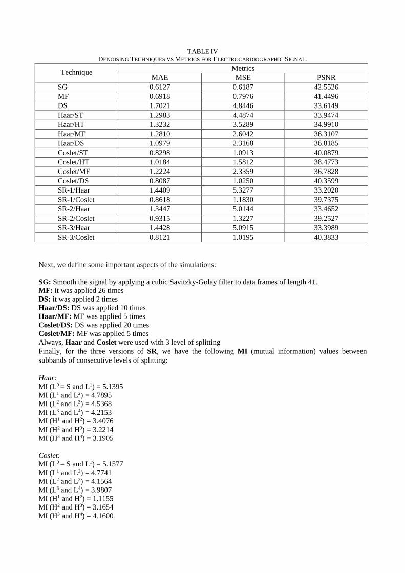
TABLE IV

DENOISING TECHNIQUES VS METRICS FOR ELECTROCARDIOGRAPHIC SIGNAL.

Technique Metrics

MAE MSE PSNR

SG 0.6127 0.6187 42.5526

MF 0.6918 0.7976 41.4496

DS 1.7021 4.8446 33.6149

Haar/ST 1.2983 4.4874 33.9474

Haar/HT 1.3232 3.5289 34.9910

Haar/MF 1.2810 2.6042 36.3107

Haar/DS 1.0979 2.3168 36.8185

Coslet/ST 0.8298 1.0913 40.0879

Coslet/HT 1.0184 1.5812 38.4773

Coslet/MF 1.2224 2.3359 36.7828

Coslet/DS 0.8087 1.0250 40.3599

SR-1/Haar 1.4409 5.3277 33.2020

SR-1/Coslet 0.8618 1.1830 39.7375

SR-2/Haar 1.3447 5.0144 33.4652

SR-2/Coslet 0.9315 1.3227 39.2527

SR-3/Haar 1.4428 5.0915 33.3989

SR-3/Coslet 0.8121 1.0195 40.3833

Next, we define some important aspects of the simulations:

SG: Smooth the signal by applying a cubic Savitzky-Golay filter to data frames of length 41.

MF: it was applied 26 times

DS: it was applied 2 times

Haar/DS: DS was applied 10 times

Haar/MF: MF was applied 5 times

Coslet/DS: DS was applied 20 times

Coslet/MF: MF was applied 5 times

Always, Haar and Coslet were used with 3 level of splitting

Finally, for the three versions of SR, we have the following MI (mutual information) values between

subbands of consecutive levels of splitting:

Haar:

MI (L0 = S and L1) = 5.1395

MI (L1 and L2) = 4.7895

MI (L2 and L3) = 4.5368

MI (L3 and L4) = 4.2153

MI (H1 and H2) = 3.4076

MI (H2 and H3) = 3.2214

MI (H3 and H4) = 3.1905

Coslet:

MI (L0 = S and L1) = 5.1577

MI (L1 and L2) = 4.7741

MI (L2 and L3) = 4.1564

MI (L3 and L4) = 3.9807

MI (H1 and H2) = 1.1155

MI (H2 and H3) = 3.1654

MI (H3 and H4) = 4.1600

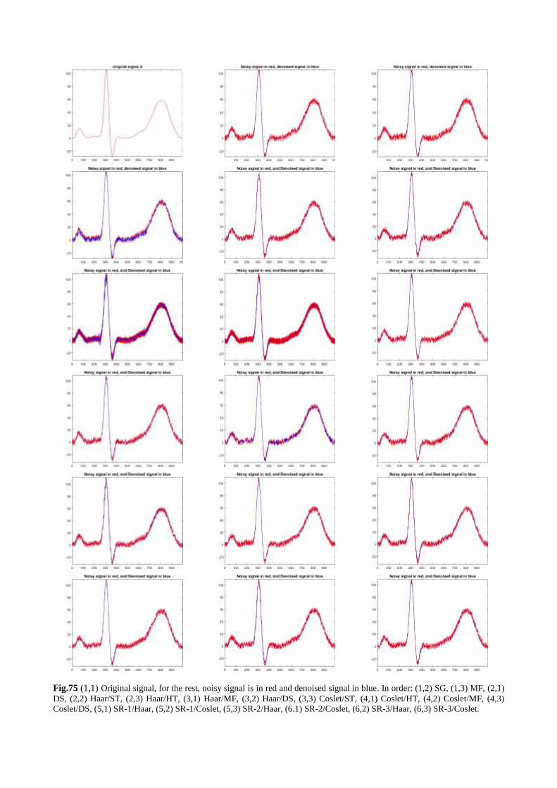
Fig.75 (1,1) Original signal, for the rest, noisy signal is in red and denoised signal in blue. In order: (1,2) SG, (1,3) MF, (2,1)

DS, (2,2) Haar/ST, (2,3) Haar/HT, (3,1) Haar/MF, (3,2) Haar/DS, (3,3) Coslet/ST, (4,1) Coslet/HT, (4,2) Coslet/MF, (4,3)

Coslet/DS, (5,1) SR-1/Haar, (5,2) SR-1/Coslet, (5,3) SR-2/Haar, (6.1) SR-2/Coslet, (6,2) SR-3/Haar, (6,3) SR-3/Coslet.

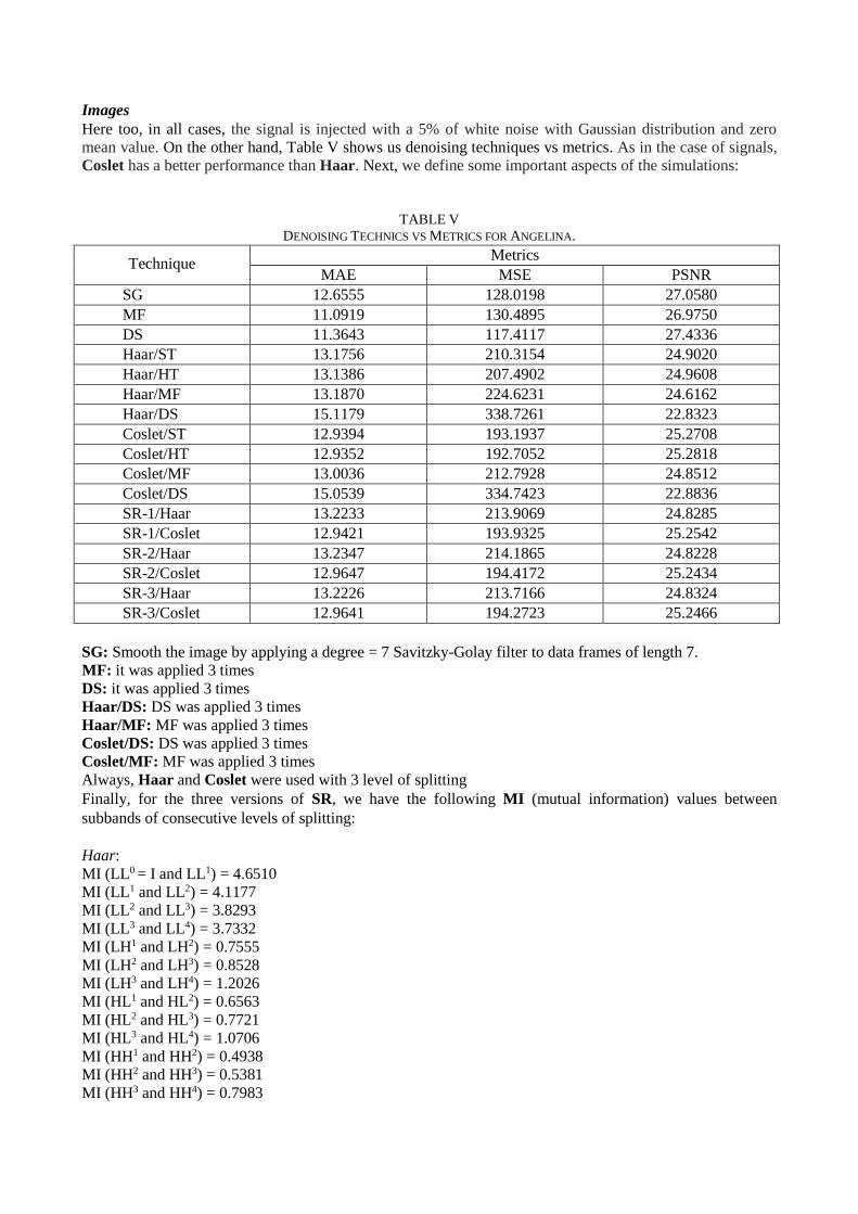
Images

Here too, in all cases, the signal is injected with a 5% of white noise with Gaussian distribution and zero

mean value. On the other hand, Table V shows us denoising techniques vs metrics. As in the case of signals,

Coslet has a better performance than Haar. Next, we define some important aspects of the simulations:

TABLE V

DENOISING TECHNICS VS METRICS FOR ANGELINA.

Technique Metrics

MAE MSE PSNR

SG 12.6555 128.0198 27.0580

MF 11.0919 130.4895 26.9750

DS 11.3643 117.4117 27.4336

Haar/ST 13.1756 210.3154 24.9020

Haar/HT 13.1386 207.4902 24.9608

Haar/MF 13.1870 224.6231 24.6162

Haar/DS 15.1179 338.7261 22.8323

Coslet/ST 12.9394 193.1937 25.2708

Coslet/HT 12.9352 192.7052 25.2818

Coslet/MF 13.0036 212.7928 24.8512

Coslet/DS 15.0539 334.7423 22.8836

SR-1/Haar 13.2233 213.9069 24.8285

SR-1/Coslet 12.9421 193.9325 25.2542

SR-2/Haar 13.2347 214.1865 24.8228

SR-2/Coslet 12.9647 194.4172 25.2434

SR-3/Haar 13.2226 213.7166 24.8324

SR-3/Coslet 12.9641 194.2723 25.2466

SG: Smooth the image by applying a degree = 7 Savitzky-Golay filter to data frames of length 7.

MF: it was applied 3 times

DS: it was applied 3 times

Haar/DS: DS was applied 3 times

Haar/MF: MF was applied 3 times

Coslet/DS: DS was applied 3 times

Coslet/MF: MF was applied 3 times

Always, Haar and Coslet were used with 3 level of splitting

Finally, for the three versions of SR, we have the following MI (mutual information) values between

subbands of consecutive levels of splitting:

Haar:

MI (LL0 = I and LL1) = 4.6510

MI (LL1 and LL2) = 4.1177

MI (LL2 and LL3) = 3.8293

MI (LL3 and LL4) = 3.7332

MI (LH1 and LH2) = 0.7555

MI (LH2 and LH3) = 0.8528

MI (LH3 and LH4) = 1.2026

MI (HL1 and HL2) = 0.6563

MI (HL2 and HL3) = 0.7721

MI (HL3 and HL4) = 1.0706

MI (HH1 and HH2) = 0.4938

MI (HH2 and HH3) = 0.5381

MI (HH3 and HH4) = 0.7983

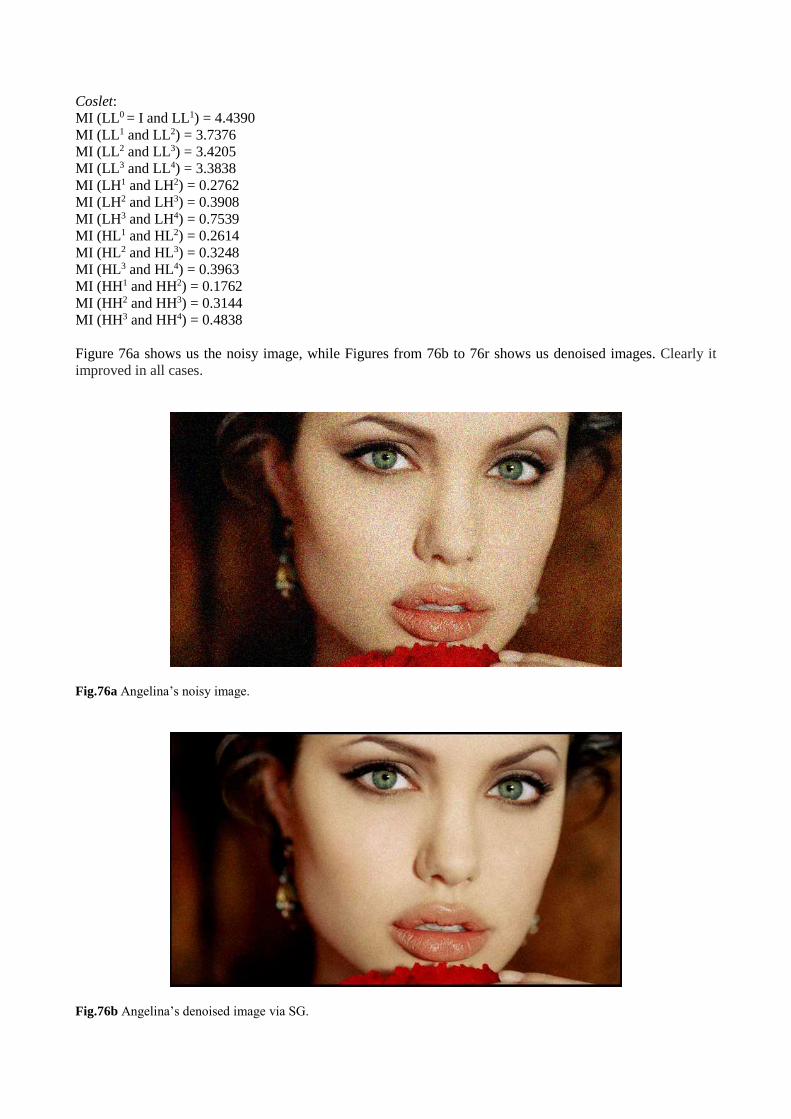
Coslet:

MI (LL0 = I and LL1) = 4.4390

MI (LL1 and LL2) = 3.7376

MI (LL2 and LL3) = 3.4205

MI (LL3 and LL4) = 3.3838

MI (LH1 and LH2) = 0.2762

MI (LH2 and LH3) = 0.3908

MI (LH3 and LH4) = 0.7539

MI (HL1 and HL2) = 0.2614

MI (HL2 and HL3) = 0.3248

MI (HL3 and HL4) = 0.3963

MI (HH1 and HH2) = 0.1762

MI (HH2 and HH3) = 0.3144

MI (HH3 and HH4) = 0.4838

Figure 76a shows us the noisy image, while Figures from 76b to 76r shows us denoised images. Clearly it

improved in all cases.

Fig.76a Angelina’s noisy image.

Fig.76b Angelina’s denoised image via SG.

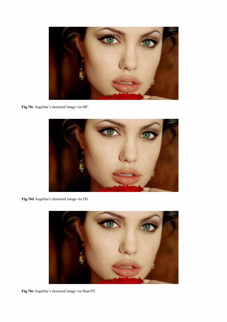
Fig.76c Angelina’s denoised image via MF.

Fig.76d Angelina’s denoised image via DS.

Fig.76e Angelina’s denoised image via Haar/ST.

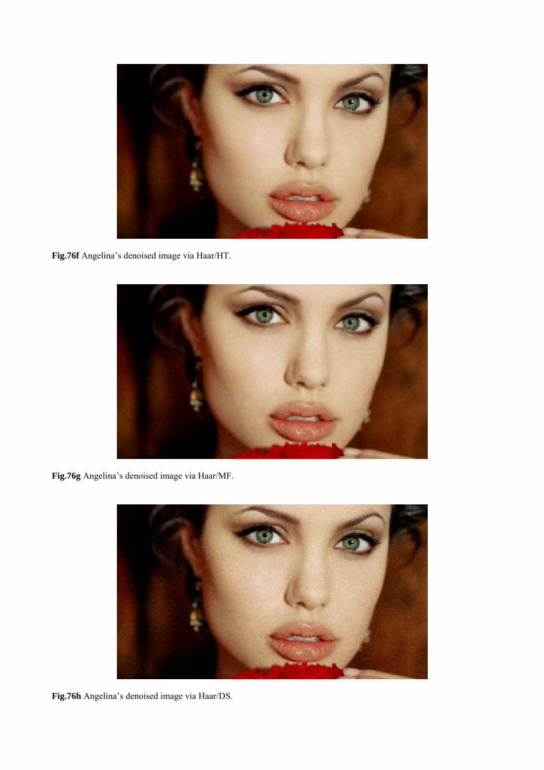
Fig.76f Angelina’s denoised image via Haar/HT.

Fig.76g Angelina’s denoised image via Haar/MF.

Fig.76h Angelina’s denoised image via Haar/DS.

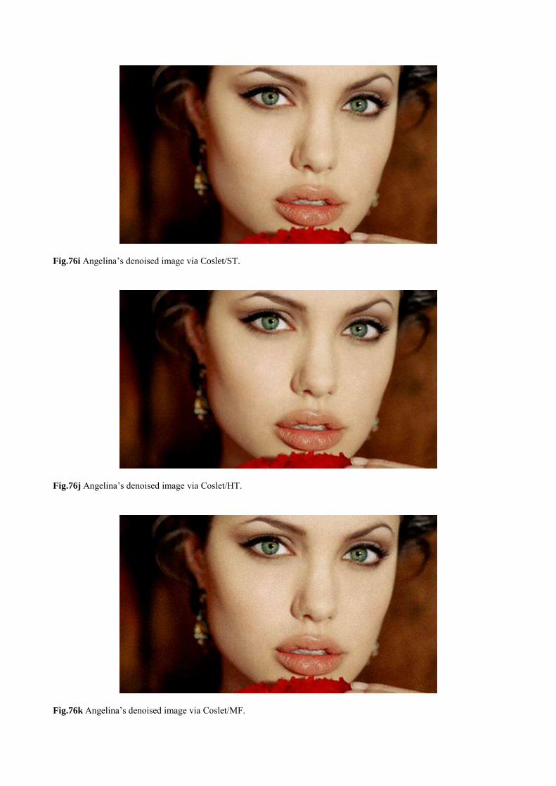
Fig.76i Angelina’s denoised image via Coslet/ST.

Fig.76j Angelina’s denoised image via Coslet/HT.

Fig.76k Angelina’s denoised image via Coslet/MF.

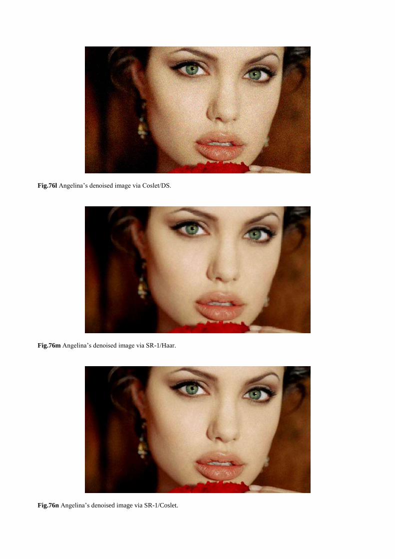
Fig.76l Angelina’s denoised image via Coslet/DS.

Fig.76m Angelina’s denoised image via SR-1/Haar.

Fig.76n Angelina’s denoised image via SR-1/Coslet.

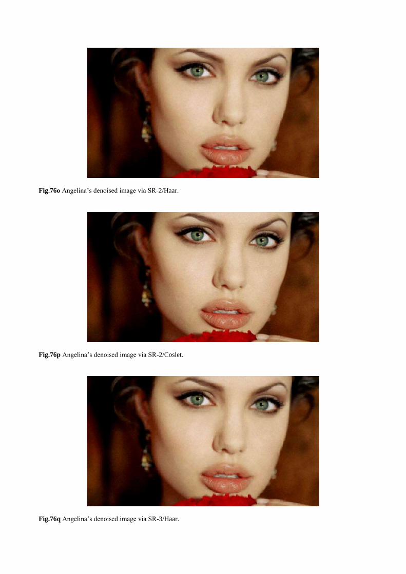
Fig.76o Angelina’s denoised image via SR-2/Haar.

Fig.76p Angelina’s denoised image via SR-2/Coslet.

Fig.76q Angelina’s denoised image via SR-3/Haar.

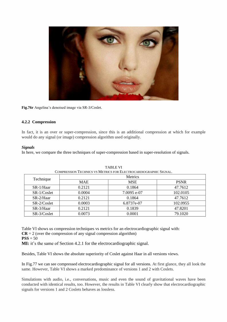
Fig.76r Angelina’s denoised image via SR-3/Coslet.

4.2.2 Compression

In fact, it is an over or super-compression, since this is an additional compression at which for example

would do any signal (or image) compression algorithm used originally.

Signals

In here, we compare the three techniques of super-compression based in super-resolution of signals.

TABLE VI

COMPRESSION TECHNICS VS METRICS FOR ELECTROCARDIOGRAPHIC SIGNAL.

Technique Metrics

MAE MSE PSNR

SR-1/Haar 0.2121 0.1864 47.7612

SR-1/Coslet 0.0004 7.0095 e-07 102.0105

SR-2/Haar 0.2121 0.1864 47.7612

SR-2/Coslet 0.0003 6.8737e-07 102.0955

SR-3/Haar 0.2121 0.1839 47.8201

SR-3/Coslet 0.0073 0.0001 79.1020

Table VI shows us compression techniques vs metrics for an electrocardiographic signal with:

CR = 2 (over the compression of any signal compression algorithm)

PSS = 50

MI: it’s the same of Section 4.2.1 for the electrocardiographic signal.

Besides, Table VI shows the absolute superiority of Coslet against Haar in all versions views.

In Fig.77 we can see compressed electrocardiographic signal for all versions. At first glance, they all look the

same. However, Table VI shows a marked predominance of versions 1 and 2 with Coslets.

Simulations with audio, i.e., conversations, music and even the sound of gravitational waves have been

conducted with identical results, too. However, the results in Table VI clearly show that electrocardiographic

signals for versions 1 and 2 Coslets behaves as lossless.

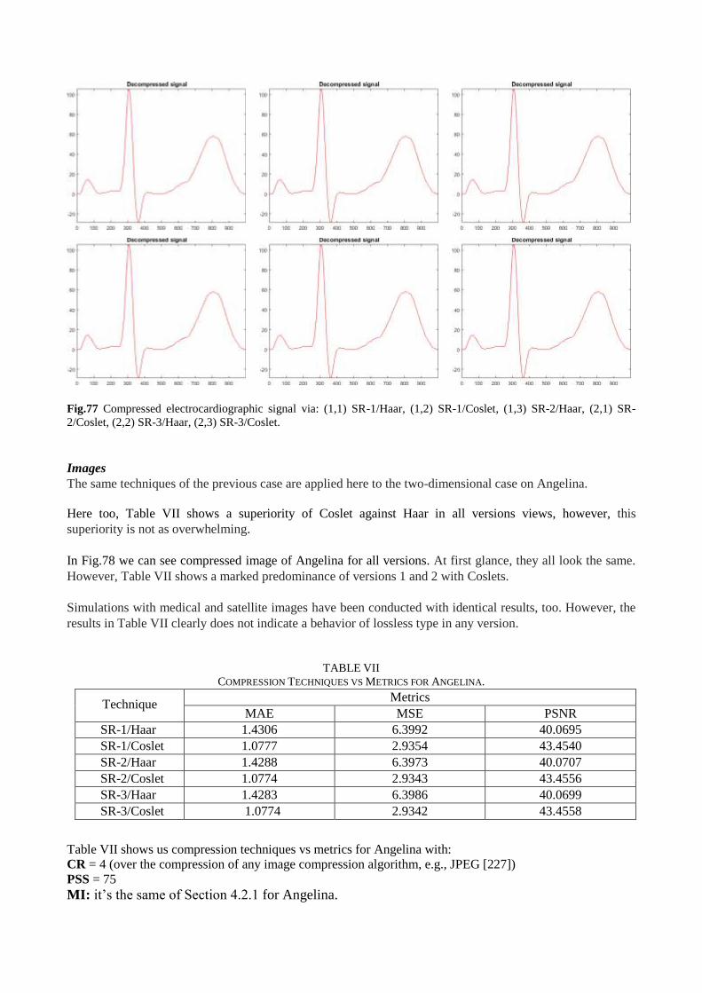
Fig.77 Compressed electrocardiographic signal via: (1,1) SR-1/Haar, (1,2) SR-1/Coslet, (1,3) SR-2/Haar, (2,1) SR-

2/Coslet, (2,2) SR-3/Haar, (2,3) SR-3/Coslet.

Images

The same techniques of the previous case are applied here to the two-dimensional case on Angelina.

Here too, Table VII shows a superiority of Coslet against Haar in all versions views, however, this

superiority is not as overwhelming.

In Fig.78 we can see compressed image of Angelina for all versions. At first glance, they all look the same.

However, Table VII shows a marked predominance of versions 1 and 2 with Coslets.

Simulations with medical and satellite images have been conducted with identical results, too. However, the

results in Table VII clearly does not indicate a behavior of lossless type in any version.

TABLE VII

COMPRESSION TECHNIQUES VS METRICS FOR ANGELINA.

Technique Metrics

MAE MSE PSNR

SR-1/Haar 1.4306 6.3992 40.0695

SR-1/Coslet 1.0777 2.9354 43.4540

SR-2/Haar 1.4288 6.3973 40.0707

SR-2/Coslet 1.0774 2.9343 43.4556

SR-3/Haar 1.4283 6.3986 40.0699

SR-3/Coslet 1.0774 2.9342 43.4558

Table VII shows us compression techniques vs metrics for Angelina with:

CR = 4 (over the compression of any image compression algorithm, e.g., JPEG [227])

PSS = 75

MI: it’s the same of Section 4.2.1 for Angelina.

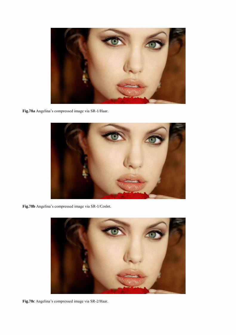
Fig.78a Angelina’s compressed image via SR-1/Haar.

Fig.78b Angelina’s compressed image via SR-1/Coslet.

Fig.78c Angelina’s compressed image via SR-2/Haar.

Fig.78d Angelina’s compressed image via SR-2/Coslet.

Fig.78e Angelina’s compressed image via SR-3/Haar.

Fig.78f Angelina’s compressed image via SR-3/Coslet.

4.2.3 Super-resolution

This technique is the decoder of the compression/decompression process of the previous section, both signals

to images.

Signals

MI: it’s the same of Section 4.2.1 for the electrocardiographic signal.

Images

MI: it’s the same of Section 4.2.1 for Angelina.

4.2.4 Edge detection

This technique was developed and simulated during this work.

Signals

In this case, this technique, i.e. FIT, it is known as flank detection, and it was seen in Section 3.3.1. There is

no equivalent to FIT in the case of signals to detect edges as in the case of images based on Roberts, Prewitt,

Sobel and Canny.

Images

Techniques of edge detection base don Roberts, Prewitt, Canny and Sobel was seen in Section 2.5, see

Fig.39. On the other hand, attributes for edge detection of FIT were seen in Sections 3.3.2 (Figures 49 to 52),

and 4.1.4 (Fig.73).

4.2.5 Hardware and Software employed

Finally, FIT was implemented in MATLAB® R2015a (Mathworks, Natick, MA) [49] on a notebook with

Intel® Core(TM) i7-4702MQ CPU @ 2.20 GHz x 2 and 8 GB RAM on Microsoft® Windows 7© Ultimate

64 bits. Besides, since all algorithms are parallelizable, distributed implementations were done on a GPU

cluster, NVIDIA® Tesla© 2050 GPU [211] with a peak performance of approximately 500 GFLOPS, with

an achieved performance of approximately 250 GFLOPS in OpenCL. The GPU needed approximately 2.5

GB of bandwidth with InfiniBand connectivity at quad data rate (QDR) QLogic® [262] or 40 Gb speeds.

5 Conclusions and future works

This work began with an extensive tour on traditional spectral techniques based on Fourier’s Theory, without

compact support and completely disconnected from the link between time and frequency, and the respon-

sibility of each flank with respect to final spectral components of a signal, image or video. For that reason

QSA/FIT was created, i.e., to cover such space and also as a complement to the aforementioned Fourier’s

Theory, in particular, FFT. A simply comparison between QSA/FIT and FFT sheds some initial conclu-

sions, which can be seen in Table VIII.

Moreover, when the wave function collapses, we pass from QSA to FIT. This point is essential, because of

this begins to be necessary to use the Hadamard’s quotient of vectors [80].

Other contributions of this work are:

1) One-dimension directional smoothing

2) One-dimension median filter

3) Coslet (which turned out to be far superior to Haar)

4) Super-resolution of signal and still images

5) Super-compression of signal and images (in fact. three versions)

6) Flank and edge detection via FIT. Etc.

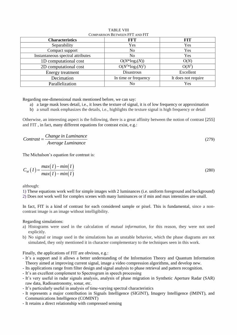
TABLE VIII

COMPARISON BETWEEN FFT AND FIT

Characteristics FFT FIT

Separability Yes Yes

Compact support No Yes

Instantaneous spectral attributes No Yes

1D computational cost O(N*log2(N)) O(N)

2D computational cost O(N2*log2(N)2) O(N2)

Energy treatment Disastrous Excellent

Decimation In time or frequency It does not require

Parallelization No Yes

Regarding one-dimensional mask mentioned before, we can say:

a) a large mask loses detail, i.e., it loses the texture of signal, it is of low frequency or approximation

b) a small mask emphasizes the details, i.e., highlights the texture signal is high frequency or detail

Otherwise, an interesting aspect is the following, there is a great affinity between the notion of contrast [255]

and FIT , in fact, many different equations for contrast exist, e.g.:

Change in LuminanceContrast

Average Luminance (279)

The Michalson’s equation for contrast is:

M

max I min IC I

max I min I

(280)

although:

1) These equations work well for simple images with 2 luminances (i.e. uniform foreground and background)

2) Does not work well for complex scenes with many luminances or if min and max intensities are small.

In fact, FIT is a kind of contrast for each considered sample or pixel. This is fundamental, since a non-

contrast image is an image without intelligibility.

Regarding simulations:

a) Histograms were used in the calculation of mutual information, for this reason, they were not used

explicitly.

b) No signal or image used in the simulations has an unstable behavior, which the phase diagrams are not

simulated, they only mentioned it in character complementary to the techniques seen in this work.

Finally, the applications of FIT are obvious, e.g.:

- It’s a support and it allows a better understanding of the Information Theory and Quantum Information

Theory aimed at improving current signal, image a video compression algorithms, and develop new.

- Its applications range from filter design and signal analysis to phase retrieval and pattern recognition.

- It’s an excellent complement to Spectrogram in speech processing

- It’s very useful in radar signals analysis, analysis of phase migration in Synthetic Aperture Radar (SAR)

raw data, Radioastronomy, sonar, etc.

- It’s particularly useful in analysis of time-varying spectral characteristics

- It represents a major contribution in Signals Intelligence (SIGINT), Imagery Intelligence (IMINT), and

Communications Intelligence (COMINT)

- It retains a direct relationship with compressed sensing

- Besides, its applications are obvious in a fine processing signal, namely: power spectral density (with a

strict sense of time); frequency-hopping spread spectrum; analysis of stationarity; time series analysis;

study of seismic signals, in general, and, earthquakes, in particular; nonlinear spectral analysis; nonlinear

sampling for a most efficient compression schema instead of linear sampling; biomedical signal and image

analysis: electrocardiograph, electroencephalography, evoked potential, brain computer interface; analysis,

synthesis, and speech recognition, Bioinformatics: Signal Processing for DNA Sequence Analysis; condi-

tioning of acoustic spaces; and Quantum Chaos.

Finally, as we have already said, it is an extraordinary tool to assess the importance of the flanks (or edges)

in a compression process weighting in real time and sample by sample (or pixel by pixel) the importance of

temporal spectral components in the final result.

References

1. Nielsen, M.A., Chuang, I.L.: Quantum Computation and Quantum Information. Cambridge University

Press, Cambridge (2004)

2. Benioff, P.A.: Quantum mechanical Hamiltonian models of Turing machines. J. Stat. Phys. 29(3), 515–

546 (1982)

3. Feynman, R.: Simulating physics with computers. Int. J. Theor. Phys. 21(6/7), 467–488 (1982)

4. Feynman, R.: Quantum mechanical computers. Opt. News 11, 11–20 (1985)

5. Deutsch, D.: Quantum theory, the Church-Turing principle, and the universal quantum Turing machine.

Proc. R. Soc. Lond. A400, 97–117 (1985)

6. Deutsch, D., Jozsa, R.: Rapid solution of problems by quantum computation. Proc. R. Soc. Lond. A439,

553–558 (1992)

7. Simon, D.: On the power of quantum computation. SIAM J. Comput. 26(5), 1474–1483 (1997)

8. Bernstein, E., Vazirani, U.: Quantum complexity theory. SIAM J. Comput. 26(5), 1411–1473 (1997)

9. Shor, P.W.: Polynomial-time algorithms for prime factorization and discrete logarithms on a quantum

computer. SIAM J. Comput. 26(5), 1484–1509 (1997), quant-ph/9508027

10. Kaye, P., Laflamme, R., Mosca, M.: An Introduction to Quantum Computing. Oxford University Press,

Oxford (2004)

11. Stolze, J., Suter, D.: Quantum Computing: A Short Course from Theory to Experiment. WILEY-VCH

Verlag GmbH & Co. KGaA, Weinheim (2007)

12. Busemeyer, J.R., Wang, Z., Townsend, J.T.: Quantum dynamics of human decision-making. J.

Math. Psychol. 50, 220–241 (2006) doi:10.1016/j.jmp.2006.01.003

13. Eldar, Y.C.: Quantum Signal Processing. Doctoral Thesis, MIT, Dec. 2001

14. Eldar, Y.C., Oppenheim, A.V.: Quantum Signal Processing. Signal Process. Mag. 19, 12–32 (2002)

15. Vlaso, A. Y.: Quantum Computations and Images Recognition. arXiv:quant-ph/9703010 (1997)

16. Schützhold, R.: Pattern recognition on a quantum computer. Phy. Rev. A 67(6), 062311 (2003)

17. Beach, G., Lomont, C., Cohen, C.: Quantum Image Processing (QImP). Proc. Appl. Imagery Pattern

Recognit. Workshop, 39-44 (2003)

18. Venegas-Andraca, S.E., Bose, S.: Storing, processing and retrieving an image using quantum

mechanics. Proc. SPIE Conf. Quantum Inf. Comput. vol. 5105, 137–147 (2003)

19. Venegas-Andraca, S.E.: Discrete Quantum Walks and Quantum Image Processing. Thesis submitted for

the degree of Doctor of Philosophy at the University of Oxford (2005)

20. Venegas-Andraca, S.E., Ball, J.L.: Processing images in entangled quantum systems. Quantum Inf.

Process. 9(1), 1-11 (2010)

21. Latorre, J.I.: Image compression and entanglement. arXiv:quant-ph/0510031 (2005)

22. Le, P.Q., Dong, F., Hirota, K.: A flexible representation of quantum images for polynomial preparation,

image compression, and processing operations. Quantum Inf. Process. 10(1), 63-84 (2011)

23. Sun, B., Le, P.Q., Iliyasu, A.M., et al.:AMulti-channel representation for images on quantum computers

using the RGB? color space. Proc. IEEE 7th Intern. Symp. Intelligent Signal Processing, 160-165

(2011)

24. Yan, F., et al.: Assessing the Similarity of Quantum Images based on Probability Measurements. 2012

IEEE Cong. Evolutionary Computation (CEC), 1-6 (2012)

25. Le, P.Q., Iliyasu, A.M., Dong, F., Hirota, K.: Efficient color transformations on quantum images. J.

Adv. Comput. Intell. Intell. Inf. 15(6), 698-706 (2011)

26. Le, P.Q., Iliyasu, A.M., Dong, F.Y., Hirota, K.: Fast Geometric Transformations on Quantum Images.

IAENG Intern. J. of Applied Mathematics. 40(3) (2010)

27. Le, P.Q., Iliyasu, A.M., Dong, F.Y., Hirota, K.: Strategies for designing geometric transformations on

quantum images. Theoretical Computer Science. 412(15), 1506-1418 (2011)

28. Srivastava, M., Panigrah, P.K.: Quantum Image Representation Through Two-Dimensional Quantum

States and Normalized Amplitude. arXiv:quant-ph/1305.2251 (2013)

29. Li, H.S., Zhu, Q.X., Lan, S., et al.: Image storage, retrieval, compression and segmentation in a

quantum system. Quantum Inf. Process. 12(6), 2269-2290 (2013)

30. Li, H.S., Zhu, Q.X. Li, M.C., et al.: Multidimensional color image storage, retrieval, and compression

based on quantum amplitudes and phases. Information Sciences. 273, 212-232 (2014)

31. Hu, B.Q., Huang, XD, Zhou, R.G. et al.: A theoretical framework for quantum image representation and

data loading scheme Science China on Information Science. 57(3),1-11 (2014)

32. Zhang, Y., Lu, K., Gao, Y., Wang, M.: NEQR: a novel enhanced quantum representation of digital

images. Quantum Inf. Process. 12(8), 2833-2860 (2013)

33. Wang, M., Lu, K., Zhang, Y.: FLPI: representation of quantum images for log-polar coordinate. Fifth

Intern. Conf. on Digital Image Processing: ICDIP’2013 (2013)

34. Zhang, Y., Lu, K., Gao, Y., Wang, M.: A novel quantum representation for log-polar images. Quantum

Inf. Process. 12(8), 3103-3126 (2013)

35. Yuan, S., Mao, X., Chen, L. et al.: Quantum digital image processing algorithms based on quantum

measurement. Optik - International Journal for Light and Electron Optics. 124(23), 6386-6390 (2013)

36. Yuan, S., Mao, X., Xue, Y., et al.: SQR: a simple quantum representation of infrared images. Quantum

Inf. Process. 13(6), 1353-1379 (2014)

37. Zhang, W.W., Gao, F., Liu B.: A quantum watermark protocol. Int. J. Theor. Phys. 52(2), 504-513

(2013)

38. Zhang, W.W., Gao, F., Liu B., et al.: A watermark strategy for quantum images based on quantum

fourier transform. Quantum Inf. Process. 12(2), 793-803 (2013)

39. Yang, Y.G., Xia, J., Jia, X., et al.: Novel image encryption/decryption based on quantum Fourier

transform and double phase encoding. Quantum Inf. Process. 12(11), 3477-3493 (2013)

40. Yang, Y.G., Jia, X., Sun, S.J., et al.: Quantum cryptographic algorithm for color images using quantum

Fourier transform and double random-phase encoding. Information Sciences. 277, 445-457 (2014)

41. Song, X.H., Niu, X.M.: Comment on: Novel image encryption/decryption based on quantum fourier

transform and double phase encoding. Quantum Inf. Process. 13(6), 1301-1304 (2014)

42. Jiang, N., Wu, W.Y., Wang, L.: The quantum realization of Arnold and Fibonacci image scrambling

Quantum Information Processing. Quantum Inf. Process. 13(5), 1223-1236 (2014)

43. Zhou, R.G., Wu, Q., Zhang, M.Q., Shen, C.Y.: Quantum image encryption and decryption algorithms

based on quantum image geometric transformations. Int. J. Theor. Phys. 52(6), 1802-1817 (2013)

44. Tseng, C.C., Hwang, T.M.: Quantum Digital Image Processing Algorithms. 16th IPPR Conf. on

Computer Vision, Graphics and Image Processing: CVGIP’2003. Kinmen, Taiwang (2003)

45. Jain, A.K.: Fundamentals of Digital Image Processing. Prentice Hall Inc., Englewood Cliffs, NJ (1989)

46. Gonzalez, R.C., Woods, R.E.: Digital Image Processing, 2nd edn. Prentice-Hall, Englewood Cliffs

(2002)

47. Gonzalez, R.C.,Woods, R.E., Eddins, S.L.: Digital Image Processing Using Matlab. Pearson Prentice

Hall, Upper Saddle River (2004)

48. Schalkoff, R.J.: Digital Image Processing and Computer Vision. Wiley, New York (1989)

49. MATLAB® R2015a (Mathworks, Natick, MA). http://www.mathworks.com/

50. Mastriani, M.: Quantum Boolean image denoising. Springer Quantum Information Processing. 14(5),

1647-1673 (2015)

51. Rivest, R., Shamir, A., Adleman, L.: A method for obtaining digital signatures and public key

cryptosystems. Commun. ACM 21, 120–126 (1978)

52. van Leeuwen, J. (ed.): Handbook of Theoretical Computer Science. Volume A: Algorithms and

Complexity. MIT Press, Cambridge (1990)

53. Bennett, C.H., Brassard, G.: Quantum cryptography: Public key distribution and coin tossing. Proc.

IEEE Intern. Confer. Computers, Systems and Signal Processing, 175–179 (1984)

54. Lo, H.-K., Zhao, Y.: Quantum Cryptography. arXiv:0803.2507v4 [quant-ph] (2008) 55. Wiesner, S.: Sigact News 15, 78 (1983)

56. Milburn, G.J.: Schrödinger's Machines. W. H. Freeman & Co. (1997)

57. Dowling, J.P., Milburn, G.J.: Quantum Technology: The Second Quantum Revolution. Phil. Trans. R.

Soc. A 361, 3655 (2003)

58. Dowling, J.P., Milburn, G.J.: Quantum Technology: The Second Quantum Revolution. arXiv:quant-

ph/0206091v1

59. Deutsch, D.: Physics, Philosophy, and Quantum Technology. Proc. Sixth Intern. Conf. Quantum

Communication, Measurement and Computing. Shapiro, J.H., Hirota, O. (eds). Rinton Press, Princeton,

NJ (2003)

60. Cappellaro, P.: Implementation of State Transfer Hamiltonians in Spin Chains with Magnetic

Resonance Techniques. Quantum State Transfer and Network Engineering, 183-222 (2014)

61. Aiello, C.D., Cappellaro, P.: Time-optimal control by a quantum actuator. Phys. Rev. A 91, 042340

(2015)

62. Cappellaro, P.: Polarizing Nuclear Spins in Silicon Carbide. Physics, 56 (2015)

63. Cappellaro, P., et al.: Fourier magnetic imaging with nanoscale resolution and compressed sensing

speed-up using electronic spins in diamond. Nature Nanotechnology advance online publication (2015)

doi:10.1038/nnano.2015.171

64. Weinstein, Y.S., Lloyd, S., Cory, D.G.: Implementation of the Quantum Fourier Transform (1999)

quant-ph arXiv:quant-ph/9906059v1

65. Preskill, J.: Chapter 5 of his lecture notes: Lecture notes on Quantum Information Theory

http://www.theory.caltech.edu/~preskill/ph229/#lecture

66. Weedbrook, C., et al.: Gaussian quantum information. Rev. Mod. Phys. 84, 621 (2012)

67. Miguéns, J.I.L.: Quantum Data Compression. Thesis submitted for the degree of Doctor of Philosophy

at the Aalborg University (2003)

68. Schumacher, B.: Quantum coding. Phys. Rev. A, 51(4), 2738-2747 (1995)

69. Boström, K., Felbinger, T.: Lossless quantum data compression and variable-length coding”, Phys. Rev.

A 65, 032313 (2002) quant-ph/0105026

70. Jozsa, R., Presnell, S.: Universal quantum information compression and degree of prior knowledge.

(2002) quant-ph/0210196.

71. Jozsa, R., Horodecki, M., Horodecki, R., Horodecki, P.: Universal Quantum Information Compression”,

Phys. Rev. Lett., 21(8), 1714-1717 (1998)

72. Wikipedia. https://en.wikipedia.org/wiki/Fourier_transform

73. Hsu, H.P.: Fourier Analysis. Simon & Schuster, New York (1970)

74. Wikipedia. https://en.wikipedia.org/wiki/Discrete_Fourier_transform

75. Tolimieri R., An M., Lu C.: Algorithms for Discrete Fourier Transform and convolution. Springer

Verlag, New York (1997)

76. Tolimieri R., An M., Lu C.: Mathematics of multidimensional Fourier Transform Algorithms. Springer

Verlag, New York (1997)

77. Briggs, W.L., Van Emden, H.: The DFT: An Owner’s Manual for the Discrete Fourier Transform.

SIAM, Philadelphia (1995)

78. Oppenheim, A.V, Willsky, A.S., Nawab, S. H.: Signals and Systems. Second Edition, Prentice Hall,

Upper Saddle River, NJ (1997)

79. Oppenheim, A.V, Schafer, R.W.: Digital Signal Processing. Prentice Hall, Englewood Cliffs, NJ (1975)

80. De Graeve, R., Parisse, B.: Symbolic algebra and Mathematics with Xcas. University of Grenoble I

(2007) https://www-fourier.ujf-grenoble.fr/~parisse/giac/cascmd_en.pdf

81. Wikipedia. https://en.wikipedia.org/wiki/Fast_Fourier_transform

82. Van Loan, C.: Computational Frameworks for the Fast Fourier Transform, SIAM (1992)

83. Heideman, M.T., Johnson, D.H., Burrus, C.S.: Gauss and the history of the fast Fourier transform. IEEE

ASSP Magazine 1(4), 14–21 (1984) doi:10.1109/MASSP.1984.1162257

84. Strang, G.: Wavelets. American Scientist 82(3), 253 (1994)

85. Dongarra, J., Sullivan, F: Guest Editors Introduction to the top 10 algorithms. Computing in Science

Engineering 2(1), 22–23 (2000) doi:10.1109/MCISE.2000.814652. ISSN 1521-9615

86. Heideman, M.T., Johnson, D.H., Burrus, C.S.: Gauss and the history of the fast Fourier transform.

Archive for History of Exact Sciences 34(3): 265–277 (1985) doi:10.1007/BF00348431. ISSN 0003-

9519

87. Yates, F.: The design and analysis of factorial experiments. Technical Communication no. 35 of the

Commonwealth Bureau of Soils (1937)

88. Danielson, G.C., Lanczos, C.: Some improvements in practical Fourier analysis and their application to

x-ray scattering from liquids. Journal of the Franklin Institute 233 (4): 365–380 (1942)

doi:10.1016/S0016-0032(42)90767-1

89. Cooley, J.W., Lewis, P.A.W., Welch, P.D.: Historical notes on the fast Fourier transform. IEEE

Transactions on Audio and Electroacoustics 15(2): 76–79 (1967) doi:10.1109/TAU.1967.1161903

90. Cooley, J.W., Tukey, J.W.: An algorithm for the machine calculation of complex Fourier series.

Mathematics of Computation 19 (90): 297–301 (1965) doi:10.1090/S0025-5718-1965-0178586-1

91. Rockmore, D.N.: The FFT: an algorithm the whole family can use. Computing in Science Engineering 2

(1): 60–64 (2000) doi:10.1109/5992.814659

92. Wikipedia. https://en.wikipedia.org/wiki/Uncertainty_principle

93. Wikipedia. https://en.wikipedia.org/wiki/Short-time_Fourier_transform

94. Sejdić, E., Djurović, I., Jiang, J.: Time-frequency feature representation using energy concentration: An

overview of recent advances. Digital Signal Processing. 19(1), 153-183 (2009)

95. Jacobsen, E., Lyons, R.: The sliding DFT. Signal Processing Magazine. 20(2), 74–80 (2003)

96. Allen, J.B.: Short Time Spectral Analysis, Synthesis, and Modification by Discrete Fourier Transform.

IEEE Trans. on Acoustics, Speech, and Signal Processing. ASSP-25 (3), 235–238 (1977)

97. https://en.wikipedia.org/wiki/Gabor_transform

98. Ding, J.J.: Time frequency analysis and wavelet transform class note, the Department of Electrical

Engineering, National Taiwan University (NTU), Taipei, Taiwan (2007)

99. Wikipedia. https://en.wikipedia.org/wiki/Fractional_Fourier_transform

100. Condon, E.U.: Immersion of the Fourier transform in a continuous group of functional transformations.

Proc. Nat. Acad. Sci. USA 23, 158–164 (1937)

101. Namias, V.: The fractional order Fourier transform and its application to quantum mechanics. J. Inst.

Appl. Math. 25, 241–265 (1980)

102. Wiener, N.: Hermitian Polynomials and Fourier Analysis. J. Mathematics and Physics 8, 70-73 (1929)

103. Almeida, L.B.: The fractional Fourier transform and time-frequency representations. IEEE Trans. Sig.

Processing 42(11), 3084–3091 (1994)

104. Tao, R., Deng, B., Zhang, W.-Q, Wang, Y.: Sampling and sampling rate conversion of band limited

signals in the fractional Fourier transform domain. IEEE Trans. on Signal Processing, 56(1), 158–171

(2008)

105. Bhandari, A., Marziliano, P.: Sampling and reconstruction of sparse signals in fractional Fourier

domain. IEEE Signal Processing Letters, 17(3), 221–224 (2010)

106. Bailey, D.H., Swarztrauber, P.N.: The fractional Fourier transform and applications. SIAM Review 33,

389-404 (1991)

107. Shi, J., Zhang, N.-T., Liu, X.-P.: A novel fractional wavelet transform and its applications. Sci. China

Inf. Sci. 55(6), 1270-1279 (2012)

108. De Bie, H.: Fourier transform and related integral transforms in superspace. (2008)

http://www.arxiv.org/abs/0805.1918

109. Fan, H.-Y., Hu, L.-Y.: Optical transformation from chirplet to fractional Fourier transformation kernel

(2009) http://www.arxiv.org/abs/0902.1800

110. Klappenecker, A., Roetteler, M.: Engineering Functional Quantum Algorithms (2002)

http://www.arxiv.org/abs/quant-ph/0208130

111. Sejdić, E., Djurović, I., Stanković, L.J.: Fractional Fourier transform as a signal processing tool: An

overview of recent developments. Signal Processing. 91(6), 1351-1369 (2011)

112. Pégard, N.C., Fleischer, J.W.: Optimizing holographic data storage using a fractional Fourier transform.

Opt. Lett. 36, 2551-2553 (2011)

113. Wikipedia. https://en.wikipedia.org/wiki/Wavelet_transform

114. Meyer, Y.: Wavelets and Operators. Cambridge: Cambridge University Press. (1992)

115. Chui, C.K.: An Introduction to Wavelets. San Diego: Academic Press. (1992)

116. Akansu, A.N., Haddad, R.A.: Multiresolution Signal Decomposition: Transforms, Subbands, Wavelets.

San Diego: Academic Press. (1992)

117. Wikipedia. https://en.wikipedia.org/wiki/JPEG_2000

118. Malmurugan, N., Shanmugam, A., Jayaraman, S., Chander, V.V.D.: A New and Novel Image

Compression Algorithm Using Wavelet Footprints. Academic Open Internet Journal. 14 (2005)

119. Ho, T.W., Jeoti, V.: A wavelet footprints-based compression scheme for ECG signals. IEEE Region 10

Conference TENCON 2004. A., 283. (2004) doi:10.1109/TENCON.2004.1414412

120. Krantz, S.G.: A Panorama of Harmonic Analysis. Mathematical Association of America. (1999)

121. Drozdov, A.: Comparison of wavelet transform and fourier transform applied to analysis of non-

stationary processes. Nanosystems: physics, chemistry, mathematics 5: 363–373. (2014)

122. Martin, E.: Novel method for stride length estimation with body area network accelerometers. IEEE

BioWireless 2011, Univ. of California, Berkeley, CA, USA, 79-82 (2011)

123. Liu, J.: Shannon wavelet spectrum analysis on truncated vibration signals for machine incipient fault

detection. Measurement Science and Technology 23 (5): 1–11 (2012) doi:10.1088/0957-

0233/23/5/055604

124. Akansu, A.N., Serdijn, W.A., Selesnick, I.W.: Emerging applications of wavelets: A review. Physical

Communication 3: 1. (2010) doi:10.1016/j.phycom.2009.07.001

125. Donoho, D.L.: De-noising by soft-thresholding. IEEE Trans. Inform. Theory. 41(3), 613-627 (1995)

126. Donoho, D.L., Johnstone, I.M.: Adapting to unknown smoothness via wavelet shrinkage. Journal of the

American Statistical Assoc. 90(432), 1200-1224 (1995)

127. Donoho, D.L., Johnstone, I.M.: Ideal spatial adaptation by wavelet shrinkage. Biometrika. 81, 425-455

(1994)

128. Daubechies, I.: Ten Lectures on Wavelets. SIAM, Philadelphia, PA (1992)

129. Daubechies, I.: Different Perspectives on Wavelets. Proceedings of Symposia in Applied Mathematics,

vol. 47, American Mathematical Society, USA (1993)

130. Mallat, S.G.: A theory for multiresolution signal decomposition: The wavelet representation. IEEE

Trans. Pattern Anal. Machine Intell. 11(7), 674–693 (1989)

131. Mallat, S.G.: Multiresolution approximations and wavelet orthonormal bases of L2 (R). Transactions of

the American Mathematical Society, 315(1), 69-87 (1989)

132. Zhang, X.-P., Desai, M.: Nonlinear adaptive noise suppression based on wavelet transform.

Proceedings of the ICASSP98, vol. 3, 1589-1592, Seattle (1998)

133. Zhang, X.-P.: Thresholding Neural Network for Adaptive Noise reduction. IEEE Transactions on

Neural Networks. 12(3), 567-584 (2001)

134. Zhang, X.-P., Desai, M.: Adaptive Denoising Based On SURE Risk. IEEE Signal Proc. Letters. 5(10),

265-267 (1998)

135. Zhang, X.-P., Luo, Z.Q.: A new time-scale adaptive denoising method based on wavelet shrinkage.

Proceedings of the ICASSP99, Phoenix, AZ., March 15-19 (1999)

136. Lang, M., Guo, H., Odegard, J., Burrus, C., Wells, R.: Noise reduction using an undecimated discrete

wavelet transform. IEEE Signal Proc. Letters, 3(1), 10-12 (1996)

137. Chipman, H., Kolaczyk, E., McCulloch, R.: Adaptive Bayesian wavelet shrinkage. J. Amer. Statist.

Assoc. 92, 1413–1421 (1997)

138. Chang, S.G., Yu, B., Vetterli, M.: Spatially adaptive wavelet thresholding with context modeling for

image denoising. IEEE Trans. Image Processing. 9(9), 1522–1531 (2000)

139. Chang, S.G., Yu, B., Vetterli, M.: Adaptive wavelet thresholding for image denoising and compression.

IEEE Trans. Image Processing. 9(9), 1532–1546 (2000)

140. Chang, S.G., Vetterli, M.: Spatial adaptive wavelet thresholding for image denoising. Proc. ICIP. vol. 1,

374–377 (1997)

141. Crouse, M.S., Nowak, R.D., Baraniuk, R.G.: Wavelet-based statistical signal processing using hidden

Markov models. IEEE Trans. Signal Processing. 46(4), 886–902 (1998)

142. Malfait, M., Roose, D.: Wavelet-based image denoising using a Markov random field a priori model.

IEEE Trans. Image Processing. 6(4), 549–565 (1997)

143. Mihcak, M.K., Kozintsev, I., Ramchandran, K., Moulin, P.: Low complexity image denoising based on

statistical modeling of wavelet coefficients. IEEE Trans. Signal Processing Lett. 6(12), 300–303 (1999)

144. Simoncelli, E.P.: Bayesian denoising of visual images in the wavelet domain. Bayesian Inference in

Wavelet Based Models. New York: Springer-Verlag, pp. 291–308 (1999)

145. Simoncelli, E., Adelson, E.: Noise removal via Bayesian wavelet coring. Proc. ICIP, vol. 1, pp. 379–382

(1996)

146. Belge, M., Kilmer, M.E., Miller, E.L.: Wavelet domain image restoration with adaptive edge-preserving

regularization. IEEE Trans. Image Processing. 9(4), 597–608 (2000)

147. Liu, J., Moulin, P.: Information-theoretic analysis of interscale and intrascale dependencies between

image wavelet coefficients. IEEE Trans. Image Processing. 10(11), 1647–1658 (2000)

148. Guo, H., Odegard, J.E., Lang, M., Gopinath, R.A., Selesnick, I., Burrus, C.S.: Speckle reduction via

wavelet shrinkage with application to SAR based ATD/R. Technical Report CML TR94-02, CML, Rice

University, Houston (1994)

149. Coifman, R.R., Donoho, D.L.: Translation-invariant de-noising. A. Antoniadis & G. Oppenheim (eds),

Lecture Notes in Statistics. Springer-Verlag. vol. 103, pp 125-150 (1995)

150. Misiti, M., Misiti, Y., Oppenheim, G., Poggi, J.M.: Wavelet Toolbox, for use with MATLAB®, User’s

guide, R2015b (2015)

http://www.mathworks.com/help/pdf_doc/wavelet/wavelet_ug.pdf

151. Burrus, C.S., Gopinath, R.A., Guo, H.: Introduction to Wavelets and Wavelet Transforms: A Primer.

Prentice Hall, New Jersey (1998)

152. Hubbard, B.B.: The World According to Wavelets: The Story of a Mathematical Technique in the

Making. A. K. Peter Wellesley Eds., Massachusetts (1996)

153. Grossman, A., Morlet, J.: Decomposition of Hardy Functions into Square Integrable Wavelets of

Constant Shape. SIAM J. App Math. vol. 15, 723-736 (1984)

154. Valens, C.: A really friendly guide to wavelets (2004)

http://perso.wanadoo.fr/polyvalens/ clemens/wavelets/wavelets.html

155. Kaiser, G.: A Friendly Guide To Wavelets. Boston: Birkhauser (1994)

156. Walker, J.S.: A Primer on Wavelets and their Scientific Applications. Chapman & Hall/CRC, New York

(1999)

157. Stollnitz, E.J., DeRose, T.D., Salesin, D.H.: Wavelets for Computer Graphics: Theory and Applications.

Morgan Kaufmann Publishers, San Francisco (1996)

158. Shen, J., Strang, G.: The zeros of the Daubechies polynomials. Proc. American Mathematical Society

(1996)

159. Yu, R., Allen, A.R., Watson, J.: An optimal wavelet thresholding for speckle noise reduction. Summer

School on Wavelets: Papers, Publisher: Silesian Technical University, Gliwice, Poland. 77-81 (1996)

160. Gao, H.Y., Bruce, A.G.: WaveShrink with firm shrinkage. Statistica Sinica. 7, 855-874 (1997)

161. Gagnon, L., Smaili, F.D.: Speckle noise reduction of airborne SAR images with Symmetric Daubechies

Wavelets. SPIE Proc. #2759. 14-24 (1996).

162. Mastriani, M., Giraldez, A.: Smoothing of coefficients in wavelet domain for speckle reduction in

Synthetic Aperture Radar images. ICGST International Journal on Graphics, Vision and Image

Processing (GVIP). 5(6), 1-8 (2005)

163. Mastriani, M., Giraldez, A.: Despeckling of SAR images in wavelet domain. GIS Development

Magazine. 9(9), 38-40 (2005)

164. Mastriani, M.: Denoising based on wavelets and deblurring via self-organizing map for Synthetic

Aperture Radar images. International Journal of Signal Processing. 2(4), 226-235 (2005)

165. Mastriani, M.: Systholic Boolean Orthonormalizer Network in Wavelet Domain for Microarray

Denoising. International Journal of Signal Processing. 2(4), 273-284 (2005)

166. Mastriani, M., Giraldez, A.: Microarrays denoising via smoothing of coefficients in wavelet domain.

International Journal of Biomedical Sciences. 1(1), 7-14 (2006)

167. Mastriani, M., Giraldez, A.: Kalman’ Shrinkage for Wavelet-Based Despeckling of SAR Images.

International Journal of Intelligent Technology. 1(3), 190-196 (2006)

168. Mastriani, M., Giraldez, A.: Neural Shrinkage for Wavelet-Based SAR Despeckling. International

Journal of Intelligent Technology. 1(3), 211-222 (2006)

169. Mastriani, M.: Fuzzy Thresholding in Wavelet Domain for Speckle Reduction in Synthetic Aperture

Radar Images. International Journal of Intelligent Technology. 1(3), 252-265 (2006)

170. Mastriani, M.: New Wavelet-Based Superresolution Algorithm for Speckle Reduction in SAR Images.

International Journal of Computer Science. 1(4), 291-298 (2006)

171. Mastriani, M., Giraldez, A.: Enhanced Directional Smoothing Algorithm for Edge-Preserving

Smoothing of Synthetic-Aperture Radar Images. Journal of Measurement Science Review. 4(3), 1-11

(2004)

172. Yu, Y., Acton, S.T.: Speckle Reducing Anisotropic Diffusion. IEEE Trans. on Image Proc. 11(11),

1260-1270 (2002)

173. Tan, H.S.: Denoising of Noise Speckle in Radar Image. B.E. Thesis, School of Information Technology

and Electrical Engineering. The University of Queensland, October 2001

174. MATLAB Central - ECG signal database - MathWorks

http://www.mathworks.com/matlabcentral/newsreader/view_thread/335510

175. Wikipedia. https://en.wikipedia.org/wiki/Savitzky-Golay_filter

176. Whittaker, E.T., Robinson, G.: The Calculus of Observations. Blackie & Son Ed. (1924)

177. Guest, P.G.: Numerical Methods of Curve Fitting. Cambridge University Press. (2012)

178. Savitzky, A., Golay, M.J.E.: Smoothing and Differentiation of Data by Simplified Least Squares

Procedures. Analytical Chemistry 36 (8): 1627–39 (1964)

179. Savitzky, A.: A Historic Collaboration. Analytical Chemistry 61 (15): 921A–3A (1989)

180. Steinier, J., Termonia, Y., Deltour, J.: Smoothing and differentiation of data by simplified least square

procedure. Analytical Chemistry 44 (11): 1906–9 (1972)

181. Larive, C.K., Sweedler, J.V.: Celebrating the 75th Anniversary of the ACS Division of Analytical

Chemistry: A Special Collection of the Most Highly Cited Analytical Chemistry Papers Published

between 1938 and 2012. Analytical Chemistry 85 (0): 4201–2 (2013)

182. Riordon, J., Zubritsky, E., Newman, A.: Top 10 Articles. Analytical Chemistry 72 (9): 24 A–329 A. (2000)

183. Press, W.H., Teukolsky, S.A., Vetterling, W.T., Flannery, B.P.: Numerical Recipes in C: The Art of

Scientific Computing. 2nd Edition. Cambridge University Press. (2002)

184. Hamming, R.W.: Digital Filters. 2nd ed. Englewood Cliffs, NJ: Prentice-Hall (1983)

185. Ziegler, H.: Applied Spectroscopy. 35:88–92 (1981)

186. Bromba, M.U.A., Ziegler, H.: Analytical Chemistry. 53:1583–1586 (1981)

187. Krumm, J.: Savitzky-Golay Filters for 2D Images. Microsoft Research (2001)

http://research.microsoft.com/en-us/um/people/jckrumm/SavGol/SavGol.htm

188. Mastriani, M.: Single frame supercompression of still images, video, High Definition TV and Digital

Cinema. International Journal of Engineering and Mathematical Sciences. 6(3), 146-162 (2010)

189. Gilman, A., Bailey, D.G., Marsland, S.R.: Interpolation Models for Image Super-resolution. Proc. 4th

IEEE International Symposium on Electronic Design, Test & Applications, DELTA 2008, Hong Kong,

55-60 (2008)

http://www.wisdom.weizmann.ac.il/~vision/single_image_SR/files/single_image_SR.pdf

190. Glassner, D., Bagon, S., Irani, M.: Super-Resolution from a Single Image.

http://graphicon.ru/oldgr/en/publications/text/LukinKrylovNasonov.pdf

191. Lukin, A., Krylov, A.S., Nasonov, A.: Image Interpolation by Super-Resolution.

192. Huang, Y.: Wavelet-based image interpolation using multilayer perceptrons. Neural Comput. & Applic.,

14, 1-10 (2005)

193. Mueller, N., Lu, Y., Do, M.N.: Image interpolation using multiscale geometric representations. Proc.

SPIE Conf. on Electronic Imaging, San Jose, USA (2007)

http://lu.seas.harvard.edu/files/yuelu/files/interp_contourlet.pdf

194. Kraus, M., Eissele, M., Strengert, M.: GPU-Based Edge-Directed Image Interpolation.

http://citeseerx.ist.psu.edu/viewdoc/summary?doi=10.1.1.69.5655

195. -. NVIDIA CUDA: Best Practices Guide, version 3.0, 2/4/2010.

http://developer.download.nvidia.com/compute/cuda/3_0/toolkit/docs/NVIDIA_CUDA_BestPracticesG

uide.pdf

196. Podlozhnyuk, V.: Image Convolution with CUDA, June 2007.

http://developer.download.nvidia.com/compute/cuda/1_1/Website/projects/convolutionSeparable/doc/co

nvolutionSeparable.pdf

197. Simek, V., Rakesh, R.: GPU Acceleration of 2D-DWT Image Compression in MATLAB with CUDA.

Proc. Second UKSIM European Symposium on Computer Modeling and Simulations. Liverpool, UK.

274-277 (2008)

198. Wittman, T.C.: Variational Approaches to Digital Zooming. Ph.D. dissertation, Dept. Math, Univ. of

Minnesota, Saint Paul, MN (2006)

199. Mastriani, M.: Denoising and compression in wavelet domain via projection onto approximation

coefficients. International Journal of Signal Processing. 5(1), 20-30 (2009)

200. Kim, C., Choi, K., Hwang, K., Beom Ra, J.: Learning-based super-resolution using a multi-resolution

wavelet approach. http://www-isl.kaist.ac.kr/Papers/IC/ic123.pdf

201. Boon, C.S., Guleryuz, O.G., Kawahara, T., Suzuki, Y.: Sparse super-resolution reconstructions of video

from mobile devices in digital TV broadcast applications. Proc. SPIE Conf. on Applications of Digital

Image Processing XXIX, in Algorithms, Architectures, and Devices, San Diego, CA, Aug. 2006.

202. Richardson, I.E.: H.264 and MPEG-4 Video Compression: Video Coding for Next Generation

Multimedia, Ed. Wiley, N.Y. (2003)

203. Goldberg, D.E.: Genetic Algorithms in Search, Optimization, and Machine Learning, Ed. Pearson, N.Y.

(1989)

204. Jain, R., Kasturi, R., Schunck, B.G.: Machine Vision. McGraw-Hill, N.Y. (1995)

205. Preskill, J.: Chapter 2, Lecture Notes of Quantum Computation (2015)

http://www.theory.caltech.edu/people/preskill/ph229/

206. Gonorovski, I.S.: Radio circuits and signals. MIR Publishers, Moscow (1986) 207. Oppenheim, A.V., Willsky, A.S., and, Nawab, S.H.: Signals and Systems, Second Edition. Upper

Saddle River, NJ: Prentice-Hall, Inc. (1997)

208. Briggs, W.L., and, Van Emden H.: The DFT: An Owner’s Manual for the Discrete Fourier Transform,

SIAM, Philadelphia (1995)

209. Oppenheim, A.V., and, Schafer, R.W.: Discrete-Time Signal Processing, Third Edition. Upper Saddle

River, NJ: Prentice-Hall, Inc. (2010)

210. Oppenheim, A.V., and, Schafer, R.W., and, Buck, J.R.: Discrete-Time Signal Processing, Second

Edition. Upper Saddle River, NJ: Prentice-Hall, Inc. (1999)

211. NVIDIA® Tesla© 2050 GPU. http://www.nvidia.com/

212. Borman, S., and, Stevenson, R.: Image sequence processing. Department, Ed. Marcel Dekker, New

York, 2003. pp. 840-879.

213. Semmlow, J.L.: Biosignal and biomedical image processing: MATLAB-Based applications, Marcel

Dekker, Inc., New York, 2004.

214. Epstein, B.R., et al: Multispectral KLT-wavelet data compression for landsat thematic mapper images.

In Data Compression Conference, pp. 200-208, Snowbird, UT, March 1992.

215. Lee, J.: Optimized quadtree for Karhunen-Loève Transform in multispectral image coding. IEEE

Transactions on Image Processing, 8(4), pp.453-461, 1999.

216. Saghri, J.A., et al: Practical Transform coding of multispectral imagery. IEEE Signal Processing

Magazine, 12, pp.32-43, 1995.

217. Kim, T-S., et al: Multispectral image data compression using classified prediction and KLT in wavelet

transform domain. IEICE Transactions on Fundam Electron Commun Comput Sci, Vol. E86-A; No.6,

pp.1492-1497, 2003.

218. Christophe, E., et al: Hyperspectral image compression: adapting SPIHT and EZW to anisotopic 3D

wavelet coding. Submitted to IEEE Transactions on Image processing, pp.1-13, 2006.

219. Rodríguez del Río, L.S.: Fast piecewise linear predictors for lossless compression of hyperspectral

imagery. Thesis for Degree in Master of Science in Electrical Engineering, University of Puerto Rico,

Mayaguez Campus, 2003.

220. -. Hyperspectral Data Compression. Edited by Giovanni Motta, Francesco Rizzo and James A. Storer,

Chapter 3, Springer, New York, 2006.

221. Wien, M.: Variable Block-Size Transforms for Hybrid Video Coding, Degree Thesis, Institut für

Nachrichtentechnik der Rheinisch-Westfälischen Technischen Hchschule Aachen, February 2004.

222. https://en.wikipedia.org/wiki/Video_codec

223. https://en.wikipedia.org/wiki/VP9

224. https://en.wikipedia.org/wiki/VP9#VP10

225. https://en.wikipedia.org/wiki/H.264/MPEG-4_AVC

226. https://en.wikipedia.org/wiki/High_Efficiency_Video_Coding

227. Miano, J.: Compressed image file formats: JPEG, PNG, GIF, XBM, BMP. ACM Press/Addison-Wesley

Publishing Co. New York, NY, USA (1999)

228. https://en.wikipedia.org/wiki/MP3

229. Khayam, S.A.: The Discrete Cosine Transform (DCT): Theory and Application Technical Report,

WAVES-TR-ECE802.602 (2003)

230. Strang, G.: The Discrete Cosine Transform. SIAM Review, Volume 41, Number 1, pp.135-147 (1999)

231. Hung, A.C., and, Meng, TH-Y: A Comparison of fast DCT algorithms. Multimedia Systems, No. 5 Vol.

2, Dec (1994)

232. Aggarwal, G., and, Gajski, D.D.: Exploring DCT Implementations. UC Irvine, Technical Report ICS-

TR-98-10, March (1998)

233. Blinn, J.F.: What's the Deal with the DCT. IEEE Computer Graphics and Applications, pp.78-83, July

(1993)

234. Chiu, C.T., and, Liu, K.J.R.: Real-Time Parallel and Fully Pipelined 2-D DCT Lattice Structures with

Application to HDTV Systems. IEEE Trans. on Circuits and Systems for Video Technology, vol. 2 pp.

25-37, March (1992)

235. Haque, M.A.: A Two-Dimensional Fast Cosine Transform. IEEE Transactions on Acoustics, Speech

and Signal Processing, vol. ASSP-33 pp. 1532-1539, December (1985)

236. Vetterli, M.: Fast 2-D Discrete Cosine Transform. Proceedings of the IEEE ICASSP'85, Tampa, FL, pp.

1538–1541, March (1985)

237. Kamangar, F.A., and, Rao, K.R.: Fast Algorithms for the 2-D Discrete Cosine Transform. IEEE

Transactions on Computers, vol. 31 Issue 9, pp.899-906, September (1982)

238. Linzer, E.N., and, Feig, E.: New Scaled DCT Algorithms for Fused Multiply/Add Architectures.

ICASSP '91, pp.2201-2204 (1991)

239. Loeffler, C., Ligtenberg, A., and Moschytz, G.: Practical Fast 1-D DCT Algorithms with 11

Multiplications. ICASSP '89, pp.988-991 (1989)

240. Duhamel, P., Guillemot, C., and Carlach, J.C.: A DCT Chip based on a new Structured and

Computationally Efficient DCT Algorithm. ICCAS'90, pp.77-80 (1990)

241. Cho, N.I., and, Lee, S.U.: Fast Algorithm and Implementation of 2-D DCT. IEEE Transactions on

Circuits and Systems, vol. 38 no.3 pp.297-305, March (1991)

242. Cho, N.I., Yun, I.D., and, Lee, S.U.: A Fast Algorithm for 2-D DCT. ICASSP '91, pp.2197-2220, (1991)

243. McMillan, L., and Westover, L.: A Forward-Mapping Realization of the Inverse DCT. DCC '92, pp.219

(1992)

244. Duhamel, P., and, Guillemot, C.: Polynomial Transform Computation of the 2-D DCT. ICASSP'90, pp.

1515-1518 (1990)

245. -, The transform and data compression handbook, Edited by K.R. Rao, and P.C. Yip, CRC Press Inc.,

Boca Raton, FL, USA (2001)

246. Mastriani, M., and, Gambini, J.: Fast Cosine Transform to Increase Speed-up and Efficiency of

Karhunen-Loève Transform for Lossy Image Compression. International Journal of Engineering and

Mathematical Sciences, vol. 6, No 2, pp.82-92 (2010)

247. Britanak, B., Yip, P., and, Rao, K.R.: Discrete cosine and sine transforms: General properties, fast

algorithms and integer approximations. Academic Press, N.Y. (2006)

248. Pennebaker, W.B., and, Mitchell, J.L.: JPEG – Still Image Data Compression Standard. New York:

International Thomsan Publishing (1993)

249. Clark, R.J.: Transform Coding of Images. New York: Academic Press (1985)

250. Goldberg, D.E.: Genetic Algorithms in Search, Optimization, and Machine Learning. Ed. Pearson, N.Y.

(1989)

251. Gilman, A., Bailey, D.G., and, Marsland, S.R.: Interpolation Models for Image Super-resolution. In

Proc. 4th IEEE International Symposium on Electronic Design, Test & Applications, DELTA 2008,

Hong Kong, pp.55-60 (2008)

252. Melchiorri, C.: Automatic Control and System Theory: Analysis in the Phase Plane. Dipartimento di

Ingegneria dell’Energia Elettrica e dell’Informazione (DEI). Università di Bologna.

http://www-lar.deis.unibo.it/people/cmelchiorri/Files_ACST/05a_Phase_Plane.pdf

253. Myler, H.R., and, Weeks, A.R.: The pocket handbook of image processing algorithms in C. Prentice-

Hall, New Jersey (1193)

254. Image histogram. https://en.wikipedia.org/wiki/Image_histogram

255. Agu, E.: Digital Image Processing (CS/ECE 545). Lecture 2: Histograms and Point Operations (Part 1).

Computer Science Dept. Worcester Polytechnic Institute (WPI)

http://web.cs.wpi.edu/~emmanuel/courses/cs545/S14/slides/lecture02.pdf

256. Shih, M.Y., and, Tseng, D.C.: A wavelet-based multiresolution edge detection and tracking. Image and

Vision Computing, vol. 23, no. 4, pp. 441–451 (2005)

257. Mastriani, M.: Rule of Three for Superresolution of Still Images with Applications to Compression and

Denoising. ArXiv: 1405.0632 [cs.CV]. http://arxiv.org/abs/1405.0632 (2014)

258. Acharya, T., and, Tsai, P-S.: JPEG2000 Standard for Image Compression: Concepts, Algorithms and

VLSI Architectures, Ed. Wiley, N.Y., 2005.

259. Mutual Information. https://en.wikipedia.org/wiki/Mutual_information

260. Delpiano, J.: Fast mutual information of two images or signals. Part I. 07 Dec 2006 (Updated 23 Feb

2015) http://www.mathworks.com/matlabcentral/fileexchange/13289-fast-mutual-information-of-two-

images-or-signals

261. Delpiano, J.: Fast mutual information of two images or signals. Part II. 07 Dec 2006 (Updated 23 Feb

2015) https://www.mathworks.com/matlabcentral/fileexchange/13289-fast-mutual-information-of-two-

images-or-signals/content/hist2.m

262. QLogic® QDR Infiniband. http://www.qlogic.com/