quantum order of fermions : broken matsubara time translations and quantum order fingerprints s.i....

Quantum Order of Fermions : Broken Matsubara Time

Translations and Quantum Order Fingerprints

S.I. Mukhin

Theoretical Physics & Quantum Technologies Department, Moscow Institute for Steel & Alloys, Moscow, Russia

Serguey Brazovski Jan Zaanen

QUANTUM ORDER vs CLASSICAL ORDER

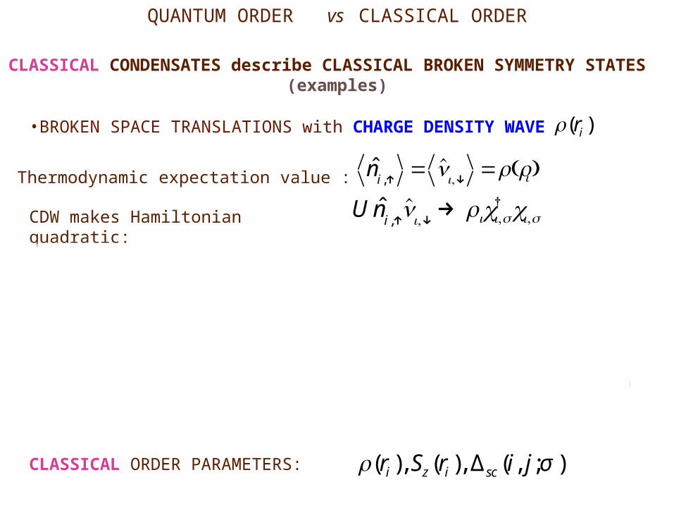
CLASSICAL CONDENSATES describe CLASSICAL BROKEN SYMMETRY STATES (examples)

•BROKEN SPACE TRANSLATIONS with CHARGE DENSITY WAVE

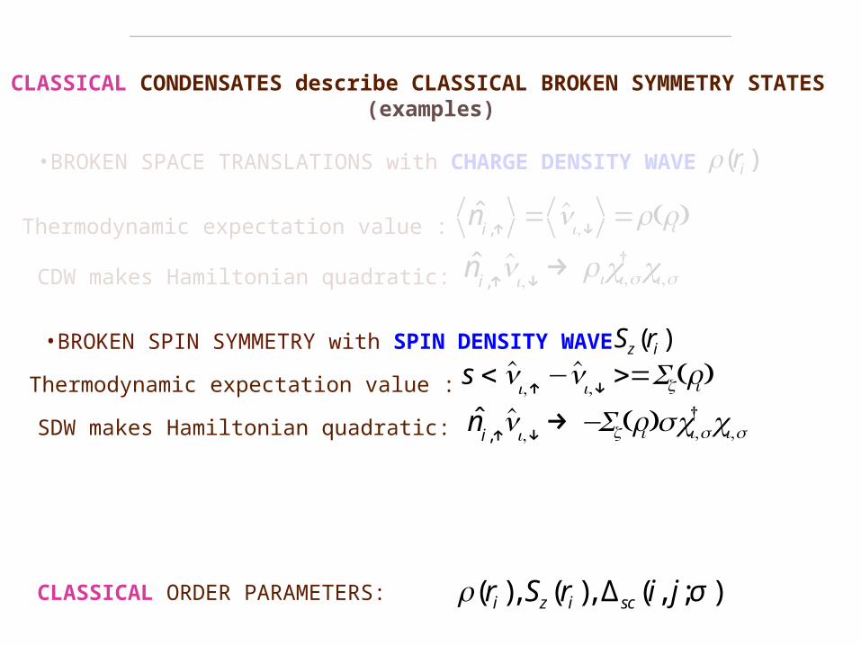
s < ni,↑ −ni,↓ >=Sz(ri )Sz (ri )

< c j ,−σ ci,σ >= Δsc (i, j;σ )Δ sc (i, j;σ )

ρ(ri )

Thermodynamic expectation value :

•BROKEN SPIN SYMMETRY with SPIN DENSITY WAVE

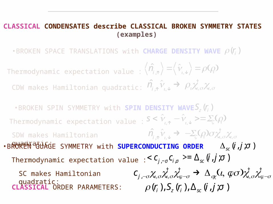
CLASSICAL ORDER PARAMETERS: ρ(ri ), Sz (ri ), Δsc (i, j;σ )



CDW makes Hamiltonian quadratic: U ni,↑ni,↓ → ρici,σ

† ci,σ

SDW makes Hamiltonian quadratic:






ρ(ri )



•BROKEN GUAGE SYMMETRY with SUPERCONDUCTING ORDER




CDW makes Hamiltonian quadratic: ni,↑ni,↓ → ρici,σ

† ci,σ







ρ(ri )



•BROKEN GUAGE SYMMETRY with SUPERCONDUCTING ORDER




CDW makes Hamiltonian quadratic: ni,↑ni,↓ → ρici,σ

† ci,σ


SC makes Hamiltonian quadratic: c j ,−σci,σci,σ† cj ,−σ

† → Δsc(i, j;σ )ci,σ† cj ,−σ

†


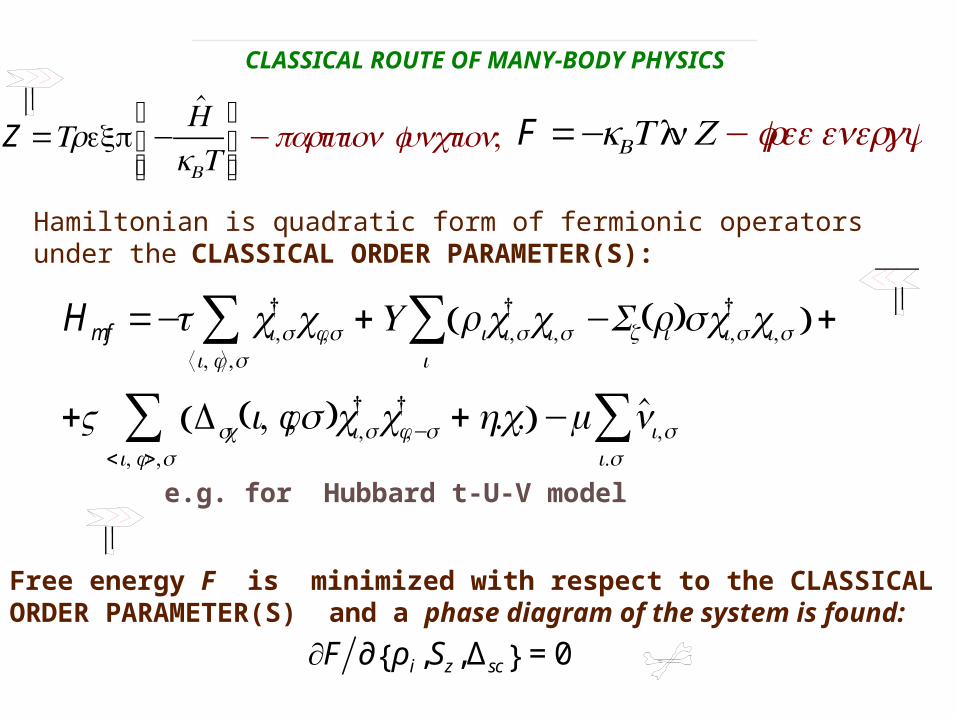
Hmf =−t ci,σ†

⟨i, j ⟩,σ∑ cj ,σ +U ρici,σ

† ci,σ −Sz(ri )σci,σ† ci,σ( )

i∑ +

+V Δsc(i, j;σ )ci,σ† cj ,−σ

† +h.c.( )<i, j>,σ∑ −μ ni,σ

i.σ∑

e.g. for Hubbard t-U-V model

Z =Trexp −H

kBT

⎧⎨⎩⎪

⎫⎬⎭⎪−partition function; F =−kBT lnZ− freeenergy

Free energy F is minimized with respect to the CLASSICAL ORDER PARAMETER(S) and a phase diagram of the system is found:

CLASSICAL ROUTE OF MANY-BODY PHYSICS

Hamiltonian is quadratic form of fermionic operators under the CLASSICAL ORDER PARAMETER(S):

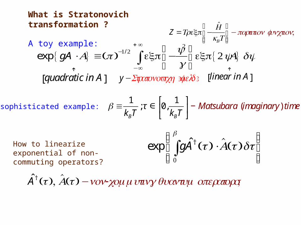
What is Stratonovich transformation ?

A toy example:

exp gA⋅A{ } ≡ π( )−1/2 exp −y2

g⎧⎨⎩

⎫⎬⎭−∞

+∞

∫ exp 2yA{ } dy↑

quadratic in A[ ]↑

linear in A[ ]y−Stratonovich 'field'

A sophisticated example:

A† τ( ), A τ( ) −non-commutingquantumoperators;

β ≡1

kBT; τ ∈ 0,

1

kBT

⎡

⎣⎢

⎤

⎦⎥− Matsubara (imaginary) time

exp gA† τ( )⋅A τ( )dτ0

β

∫⎧⎨⎪

⎩⎪

⎫⎬⎪

⎭⎪

Z =Trexp −H

kBT

⎧⎨⎩⎪

⎫⎬⎭⎪−partition function;

How to linearize exponential of non-commuting operators?

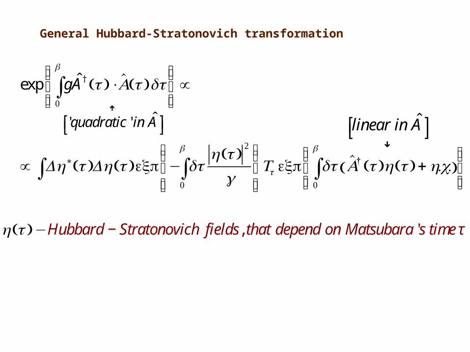
η τ( )−Hubbard − Stratonovich fields, that depend on Matsubara 's time τ

exp gA† τ( )⋅A τ( )dτ0

β

∫⎧⎨⎪

⎩⎪

⎫⎬⎪

⎭⎪∝

∝ Dη∗ τ( )∫ Dη τ( )exp − dτ0

β

∫η τ( )

2

g

⎧⎨⎪

⎩⎪

⎫⎬⎪

⎭⎪Tτ exp dτ

0

β

∫ A† τ( )η τ( ) +h.c.( )⎧⎨⎪

⎩⎪

⎫⎬⎪

⎭⎪

General Hubbard-Stratonovich transformation

↑

'quadratic ' in A⎡⎣ ⎤⎦↓

linear in A⎡⎣ ⎤⎦

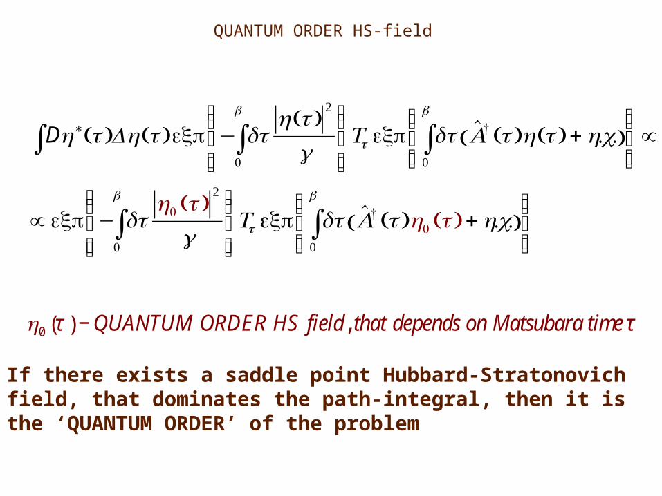
η0 τ( ) −QUANTUM ORDER HS field, that depends on Matsubara time τ

Dη∗ τ( )∫ Dη τ( )exp − dτ0

β

∫η τ( )

2

g

⎧⎨⎪

⎩⎪

⎫⎬⎪

⎭⎪Tτ exp dτ

0

β

∫ A† τ( )η τ( ) +h.c.( )⎧⎨⎪

⎩⎪

⎫⎬⎪

⎭⎪∝

∝ exp − dτ0

β

∫η0 τ( )

2

g

⎧⎨⎪

⎩⎪

⎫⎬⎪

⎭⎪Tτ exp dτ

0

β

∫ A† τ( )η0 τ( ) +h.c.( )⎧⎨⎪

⎩⎪

⎫⎬⎪

⎭⎪

If there exists a saddle point Hubbard-Stratonovich field, that dominates the path-integral, then it is the ‘QUANTUM ORDER’ of the problem

QUANTUM ORDER HS-field

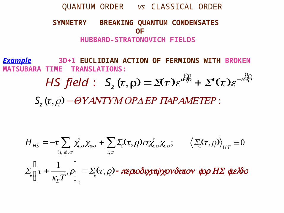
Example 3D+1 EUCLIDIAN ACTION OF FERMIONS WITH BROKEN MATSUBARA TIME TRANSLATIONS:

SYMMETRY BREAKING QUANTUM CONDENSATES OF

HUBBARD-STRATONOVICH FIELDS

HHS =−t ci,σ†

⟨i, j ⟩,σ∑ cj ,σ + Sz(τ ,ri )

i,σ∑ σci,σ

† ci,σ ; Sz(τ ,ri ) 1/T≡0

Sz τ +1

kBT,r

⎛

⎝⎜⎞

⎠⎟i

=Sz(τ ,ri )- periodicitycondition for HS fields


HS field : Sz (τ,r) =S(τ )eirQrr +S∗(τ )e−i

rQrr

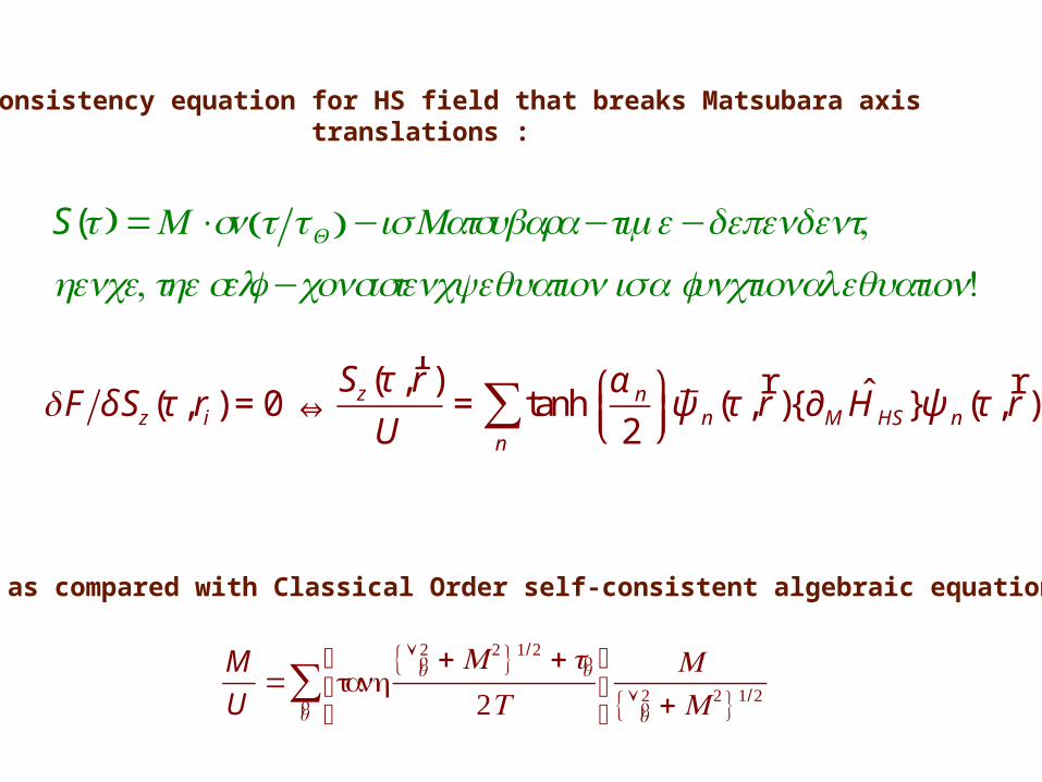
Self-consistency equation for HS field that breaks Matsubara axis translations :

δF δSz (τ ,ri ) = 0 ⇔

Sz (τ ,rr )

U= tanh

n∑

α n

2⎛⎝⎜

⎞⎠⎟ψ n (τ ,

rr ){∂M HHS}ψ n (τ ,

rr )

M

U= tanh

{Úrq2 + M 2}1/2 + tr

q

2T

⎡

⎣⎢

⎤

⎦⎥

rq∑ M

{Úrq2 + M 2}1/2

S(τ ) =M ⋅sn τ τQ( )−is Matsubara−time−dependent,

hence, theself −consistencyequationisa functional equation!

as compared with Classical Order self-consistent algebraic equation :

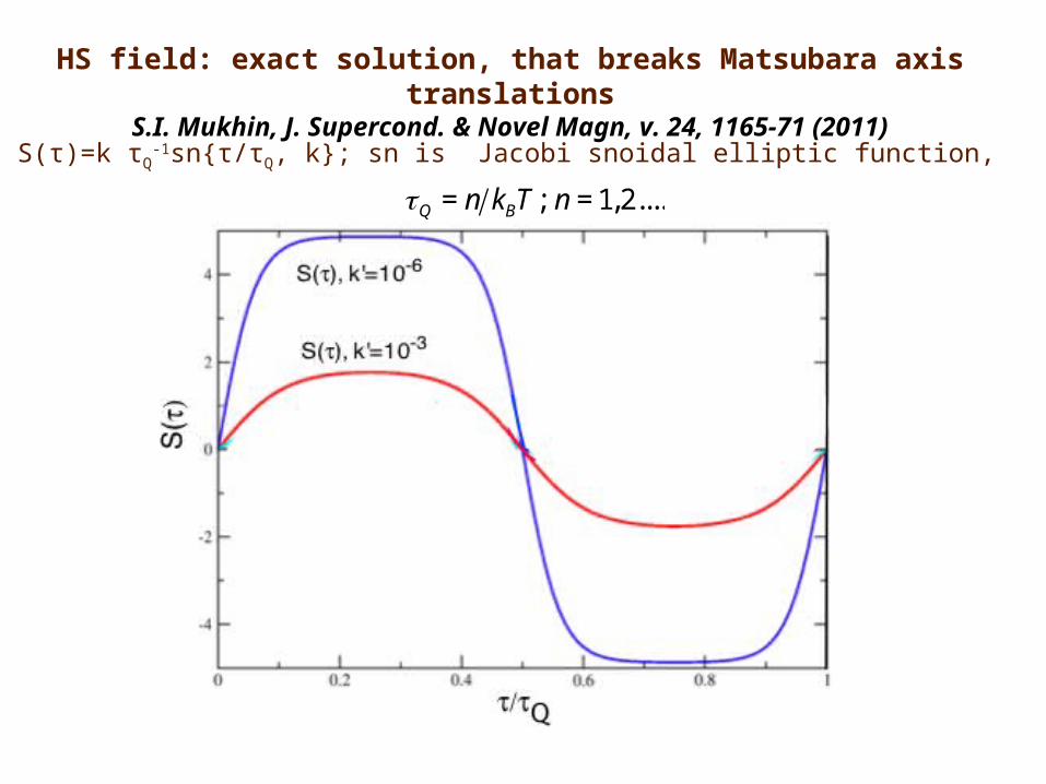
S(τ)=k τQ-1sn{τ/τQ, k}; sn is Jacobi snoidal elliptic function,

HS field: exact solution, that breaks Matsubara axis translationsS.I. Mukhin, J. Supercond. & Novel Magn, v. 24, 1165-71 (2011)

τQ = n kBT ; n = 1,2....

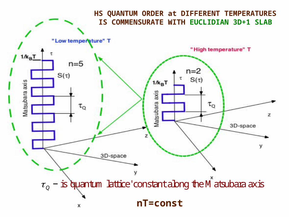
HS QUANTUM ORDER at DIFFERENT TEMPERATURESIS COMMENSURATE WITH EUCLIDIAN 3D+1 SLAB

nT=const

τQ − is 'quantum lattice' constant along the Matsubara axis

So, why quantum orders are so rare ? Or why we do not see them ?

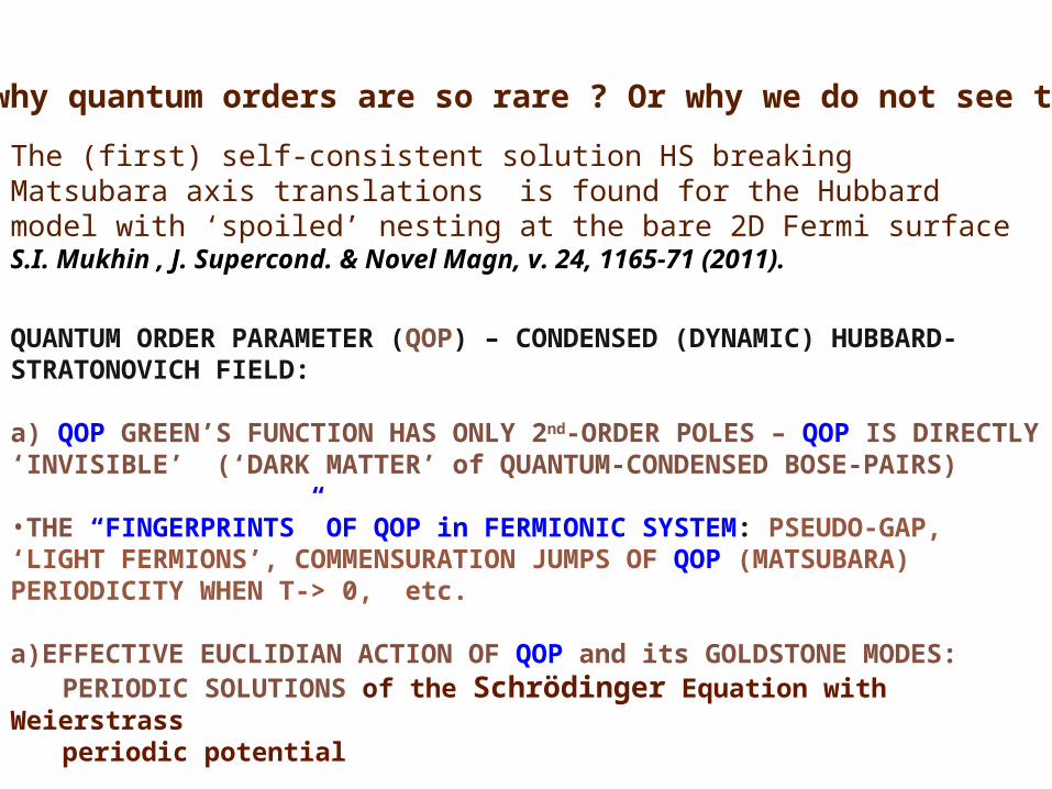
The (first) self-consistent solution HS breaking Matsubara axis translations is found for the Hubbard model with ‘spoiled’ nesting at the bare 2D Fermi surface S.I. Mukhin , J. Supercond. & Novel Magn, v. 24, 1165-71 (2011).

QUANTUM ORDER PARAMETER (QOP) – CONDENSED (DYNAMIC) HUBBARD-STRATONOVICH FIELD:

a) QOP GREEN’S FUNCTION HAS ONLY 2nd-ORDER POLES – QOP IS DIRECTLY ‘INVISIBLE’ (‘DARK MATTER’ of QUANTUM-CONDENSED BOSE-PAIRS)

•THE “FINGERPRINTS” OF QOP in FERMIONIC SYSTEM: PSEUDO-GAP, ‘LIGHT FERMIONS’, COMMENSURATION JUMPS OF QOP (MATSUBARA) PERIODICITY WHEN T-> 0, etc.

a)EFFECTIVE EUCLIDIAN ACTION OF QOP and its GOLDSTONE MODES: PERIODIC SOLUTIONS of the Schrödinger Equation with Weierstrass periodic potential

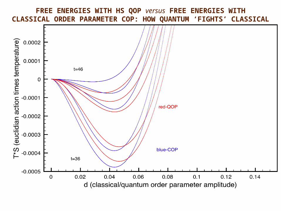
FREE ENERGIES WITH HS QOP versus FREE ENERGIES WITHCLASSICAL ORDER PARAMETER COP: HOW QUANTUM ‘FIGHTS’ CLASSICAL

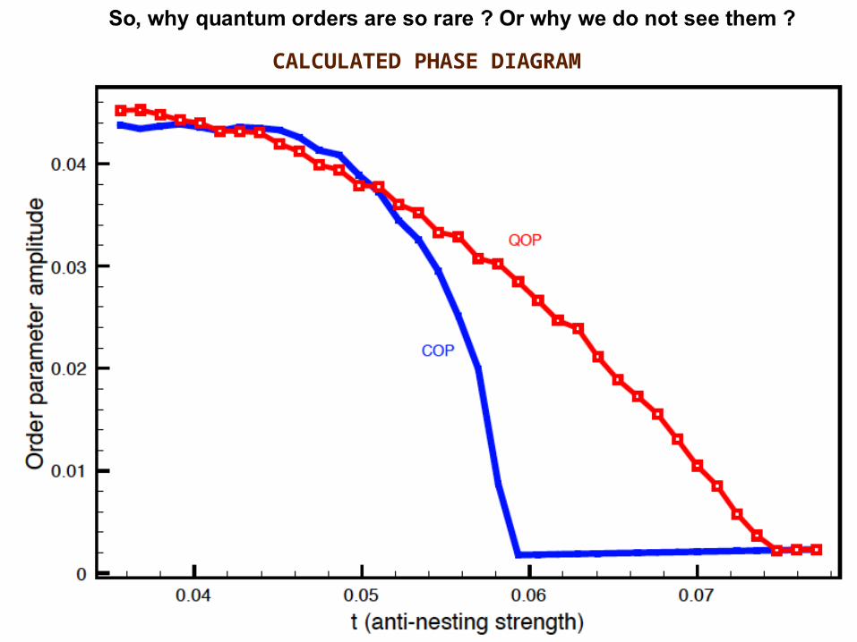
CALCULATED PHASE DIAGRAM

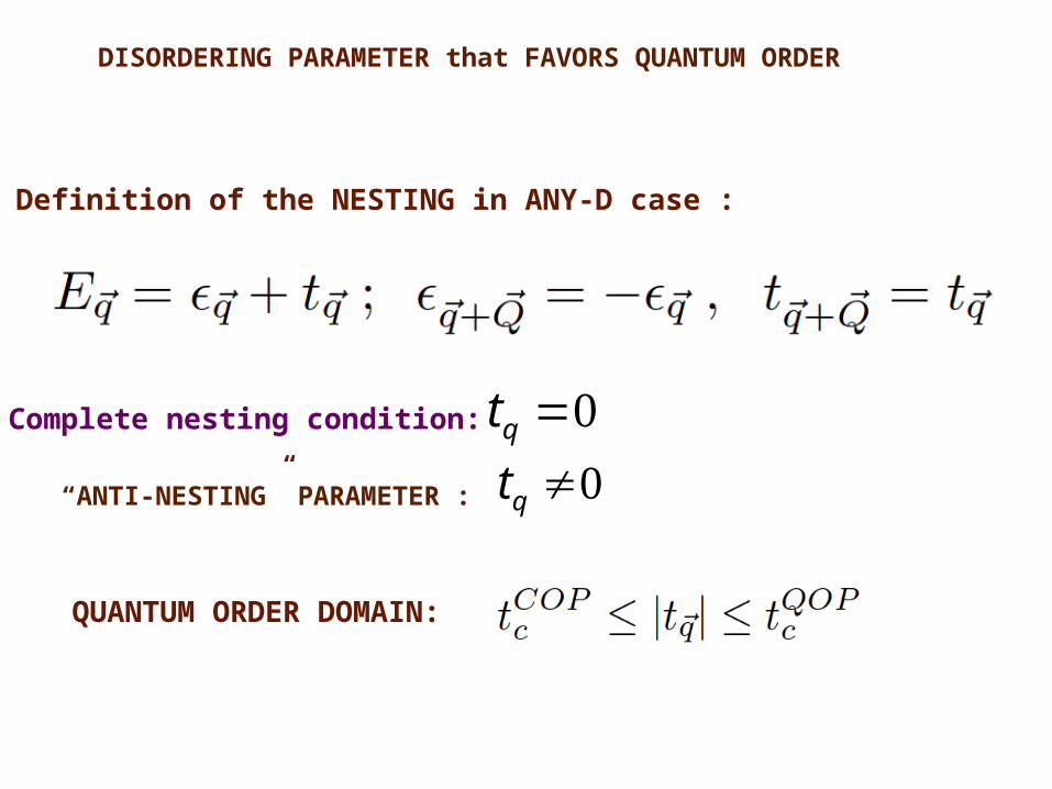
DISORDERING PARAMETER that FAVORS QUANTUM ORDER

Definition of the NESTING in ANY-D case :

tq =0Complete nesting condition:

“ANTI-NESTING” PARAMETER : tq ≠0

QUANTUM ORDER DOMAIN:

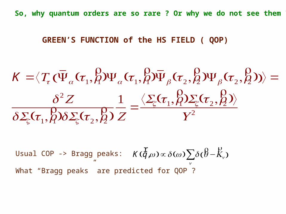
GREEN’S FUNCTION of the HS FIELD ( QOP)

K =⟨Tτ Ψα (τ1,rr1)Ψα (τ1,

rr1)Ψβ (τ 2 ,

rr2 )Ψβ (τ 2 ,

rr2 )( )⟩ =

δ 2ZδSz(τ1,

rr1)δSz(τ 2 ,

rr2 )

1Z=⟨Sz(τ1,

rr1)Sz(τ 2 ,

rr2 )⟩

U 2


Usual COP -> Bragg peaks:

What “Bragg peaks” are predicted for QOP ?

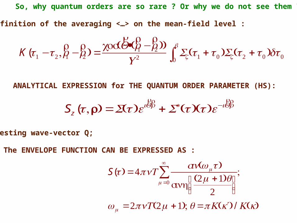
Definition of the averaging <…> on the mean-field level :

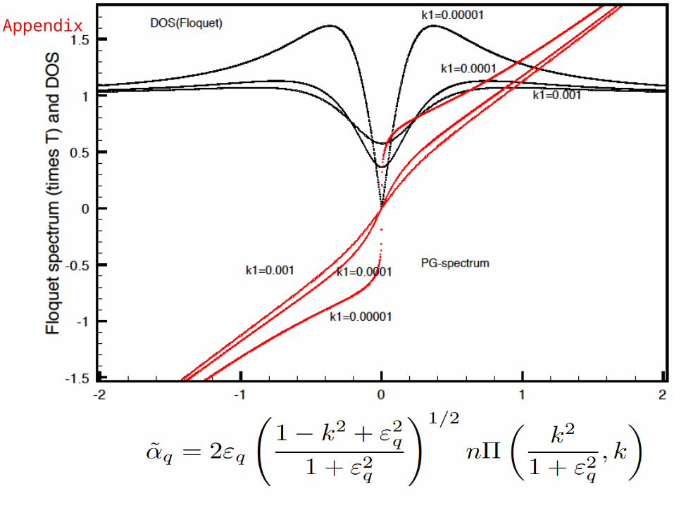
ANALYTICAL EXPRESSION for THE QUANTUM ORDER PARAMETER (HS):

nesting wave-vector Q;

The ENVELOPE FUNCTION CAN BE EXPRESSED AS :

Sz (τ,r) =S(τ )eirQrr +S∗(τ )(τ )e−i

rQrr

K(τ1 −τ 2 ,

rr1 −

rr2 ) =

cos(rQ·(

rr1 −

rr2 ))

U 2 Sz(τ1 +τ 0 )Sz(τ 2 +τ 0 )0

β

∫ dτ 0

S(τ ) =4πnTsin(ωmτ )

sinh(2m+1)q

2⎛⎝⎜

⎞⎠⎟

m=0

∞

∑ ;

ωm =2πnT(2m+1);q=πK ( ′k ) / K (k)


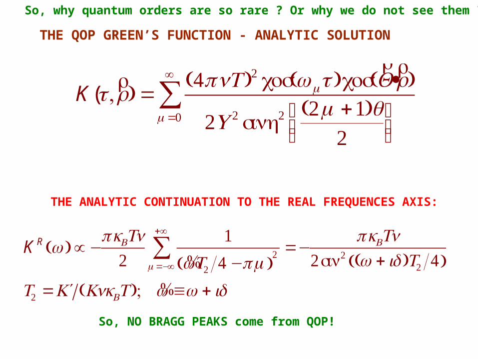
THE QOP GREEN’S FUNCTION - ANALYTIC SOLUTION

THE ANALYTIC CONTINUATION TO THE REAL FREQUENCES AXIS:

K R ω( ) ∝ −πkBTn

21

%ωT2 4 −πm( )2

m=−∞

+∞

∑ =−πkBTn

2sin2 (ω + iδ )T2 4( )

T2 = ′K (KnkBT ); %ω ≡ω + iδ

K(τ, rr ) =(4πnT )2 cos(ωmτ )cos(

rQ·

rr )

2U 2 sinh2 (2m+1)q2

⎛⎝⎜

⎞⎠⎟

m=0

∞

∑

So, why quantum orders are so rare ? Or why we do not see them ?So, why quantum orders are so rare ? Or why we do not see them ?

So, NO BRAGG PEAKS come from QOP!

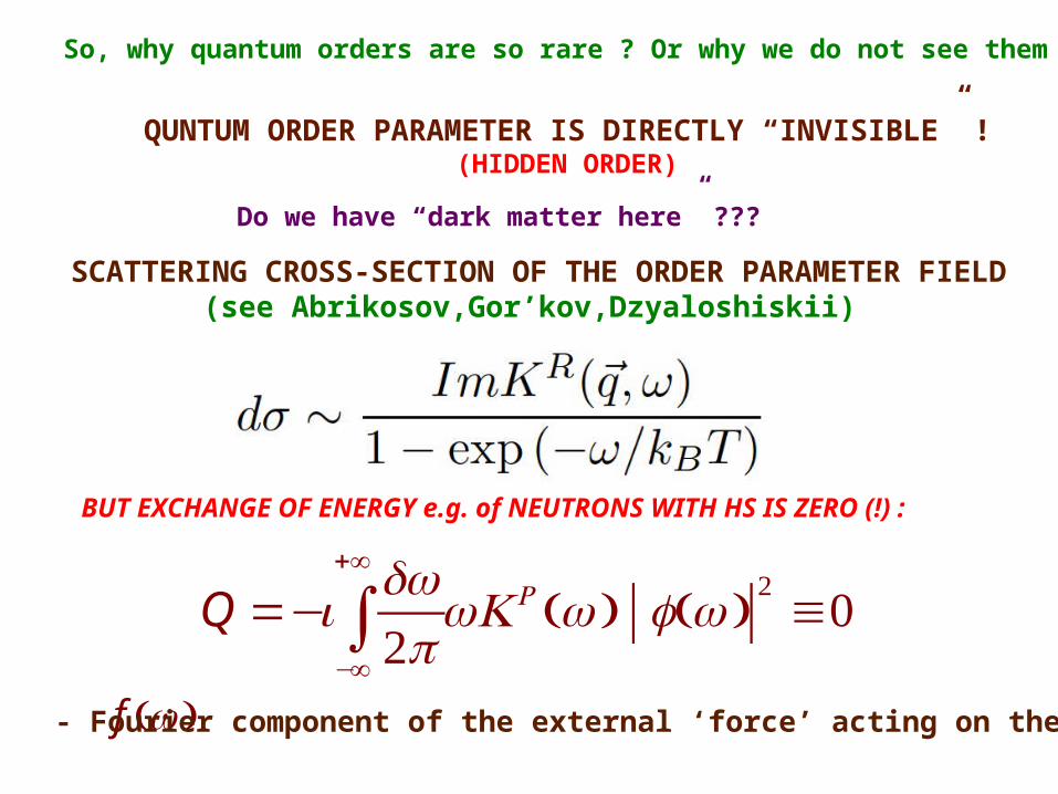
QUNTUM ORDER PARAMETER IS DIRECTLY “INVISIBLE” !(HIDDEN ORDER)

SCATTERING CROSS-SECTION OF THE ORDER PARAMETER FIELD(see Abrikosov,Gor’kov,Dzyaloshiskii)

BUT EXCHANGE OF ENERGY e.g. of NEUTRONS WITH HS IS ZERO (!) :

Q =−idω2π−∞

+∞

∫ ωK R ω( ) f ω( )2≡0

Do we have “dark matter here” ???

f ω( ) - Fourier component of the external ‘force’ acting on the HS QOP


THE “FINGERPRINTS” OF QOP in the FERMI-SYSTEM

Fermionic Greens function in the system with broken Matsubara time translations is found analytically (S.I. Mukhin, T.R. Galimzyanov, 2011, in preparation)

Timur (outside the Department)

LG =δ(τ −τ '),

L =∂τ −S τ( ) ε p

ε p ∂τ +S τ( )

⎛

⎝⎜⎜

⎞

⎠⎟⎟

G τ( ) =G11 G12

G21 G22

⎛

⎝⎜⎜

⎞

⎠⎟⎟−Matsubara−time−dependent Green's function

To find measurable predictions one has to make analytical continuation fromMatsubara to real time and derive :

−ImGR (ω, p) ∝ DOS

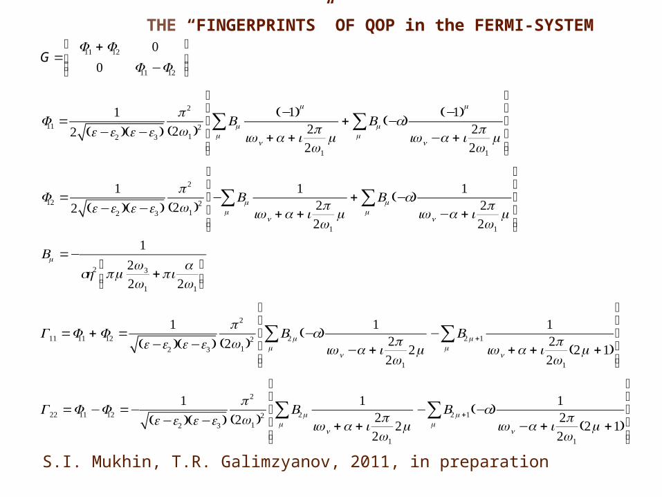
S.I. Mukhin, T.R. Galimzyanov, 2011, in preparation

G =F11 + F12 0

0 F11 −F12

⎛

⎝⎜⎜

⎞

⎠⎟⎟

F11 =1

2 (e−e2 )(e−e3)π 2

(2ω1)2 Bm

m∑ −1( )m

iωn +α + i2π2ω1

m+ Bm

m∑ (−a)

−1( )m

iωn −α + i2π2ω1

m

⎡

⎣

⎢⎢⎢⎢

⎤

⎦

⎥⎥⎥⎥

F12 =1

2 (e−e2 )(e−e3)π 2

(2ω1)2 − Bm

m∑ 1

iωn +α + i2π2ω1

m+ Bm

m∑ (−a)

1


m

⎡

⎣

⎢⎢⎢⎢

⎤

⎦

⎥⎥⎥⎥

Bm =−1

sh2 πm2ω 3

2ω1

+πia

2ω1

⎛

⎝⎜⎞

⎠⎟

G11 =F11 + F12 =1

(e−e2 )(e−e3)π 2

(2ω1)2 B2m

m∑ (−a)

1


2m− B2m+1

m∑ 1

iωn +α + i2π2ω1

(2m+1)

⎡

⎣

⎢⎢⎢⎢

⎤

⎦

⎥⎥⎥⎥

G22 =F11 −F12 =−1

(e−e2 )(e−e3)π 2

(2ω1)2 B2m

m∑ 1

iωn +α + i2π2ω1

2m− B2m+1

m∑ (−a)

1


(2m+1)

⎡

⎣

⎢⎢⎢⎢

⎤

⎦

⎥⎥⎥⎥

THE “FINGERPRINTS” OF QOP in the FERMI-SYSTEM

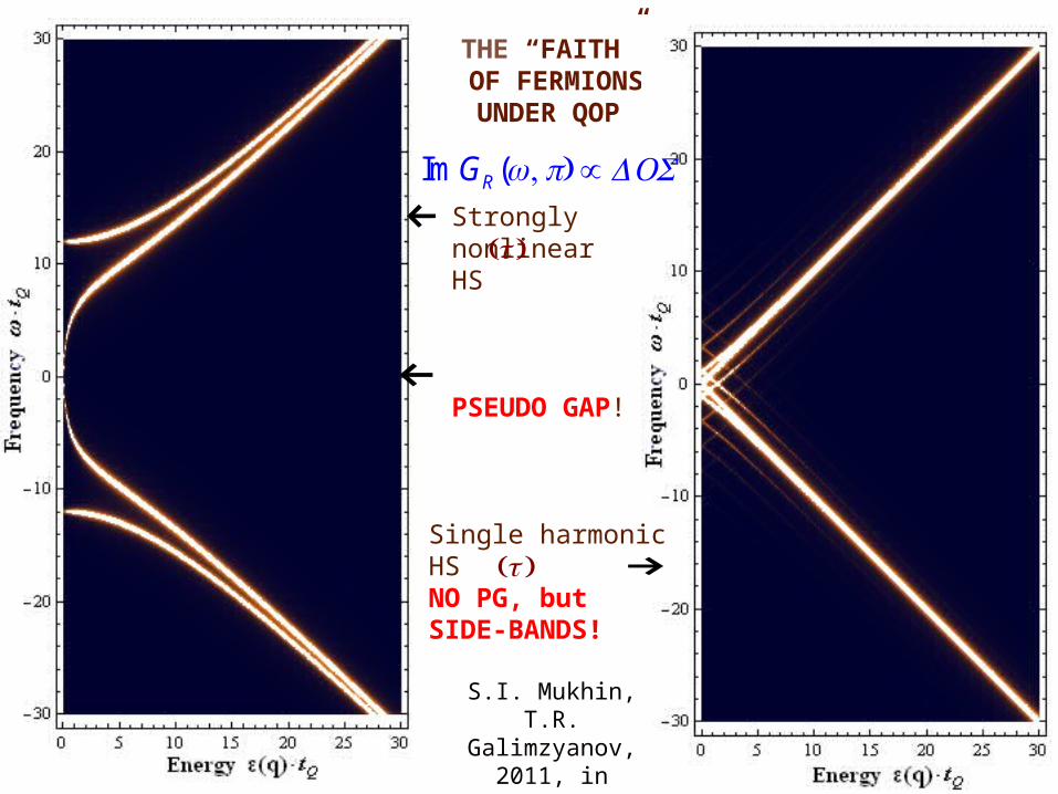
THE “FAITH” OF FERMIONS

UNDER QOP

Strongly nonlinearHS

PSEUDO GAP!

τ( )←

Single harmonicHSNO PG, butSIDE-BANDS!

τ( ) →

S.I. Mukhin, T.R. Galimzyanov, 2011,

in preparation

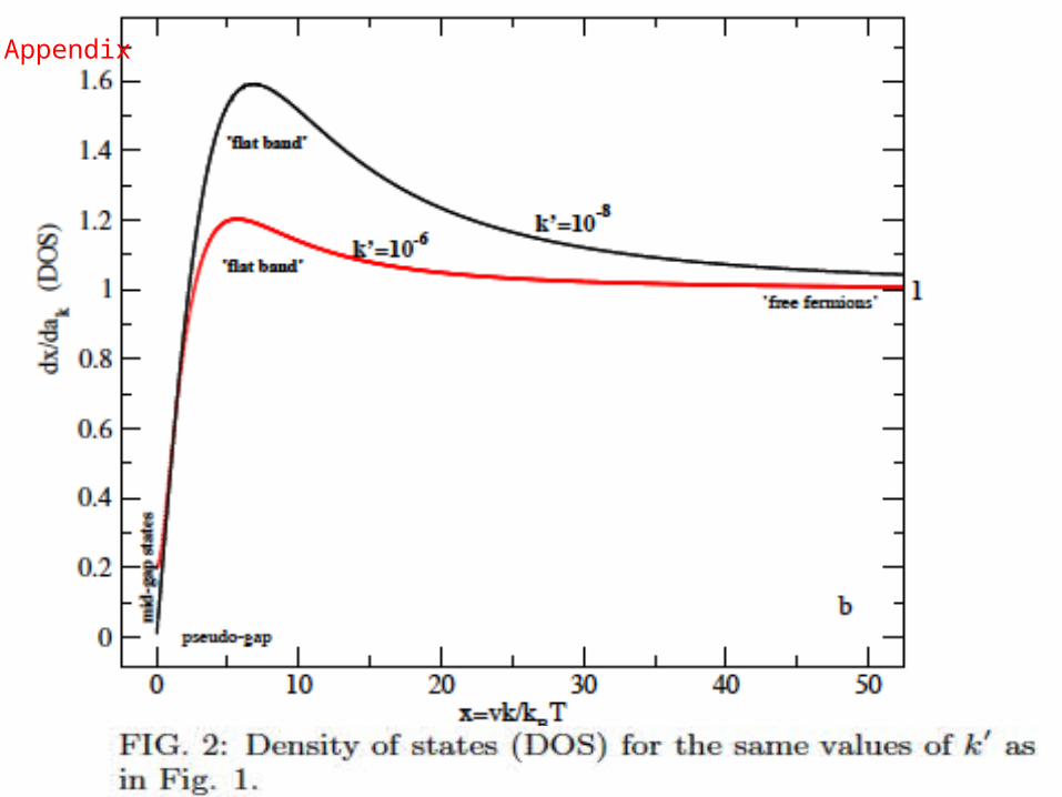
ImGR (ω, p) ∝ DOS

←

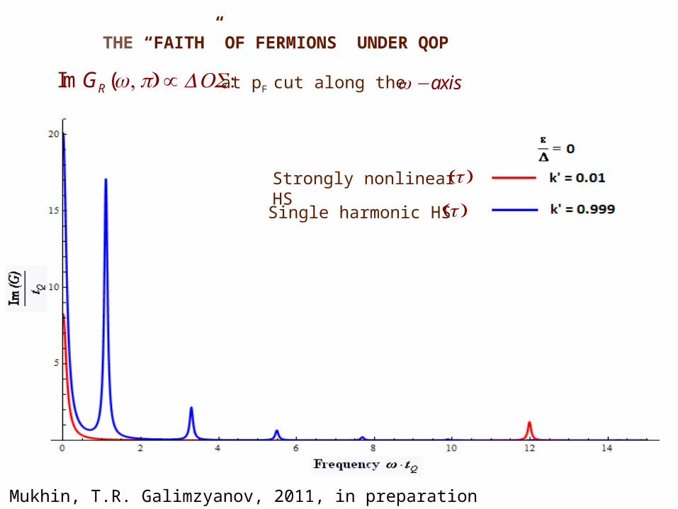
THE “FAITH” OF FERMIONS UNDER QOP

ImGR (ω, p) ∝ DOS : at pF cut along the ω −axis

Strongly nonlinear HS τ( )

Single harmonic HS τ( )

S.I. Mukhin, T.R. Galimzyanov, 2011, in preparation

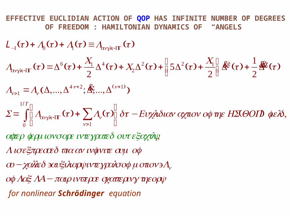
EFFECTIVE EUCLIDIAN ACTION OF QOP HAS INFINITE NUMBER OF DEGREES OF FREEDOM : HAMILTONIAN DYNAMICS OF “ANGELS”

L−1(τ ) + L0 (τ ) + L1(τ ) ≡Lsingle-PG(τ )

Lsingle-PG(τ ) =Δ6 (τ ) +C1

2Δ4 (τ ) +C2Δ

2 (τ ) + 5Δ2 (τ ) +C1

2⎛⎝⎜

⎞⎠⎟&Δ2 (τ ) +

12&&Δ2 (τ )

Ln>1 =Ln Δ,...,Δ4n+2; &Δ,...,Δ(n+1)( )

S= Lsingle-PG(τ ) + Ln(τ )n>1∑⎧

⎨⎩

⎫⎬⎭dτ

0

1/T

∫ −Euclidianactionof theHS(QOP) field,

after fermionsareintegratedout exactly,L isexpressedviaaninfinitesumofso−called 'auxiliaryintegralsof motion' Ln

of Lax LA−pair inversescatteringtheory for nonlinear Schrödinger equation

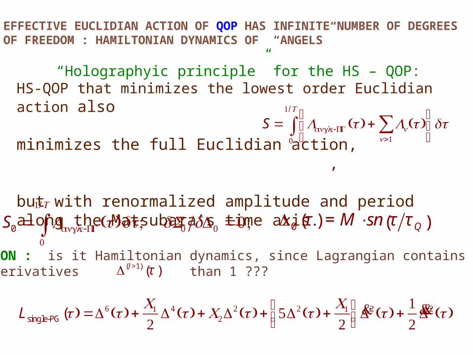
“Holographyic principle” for the HS – QOP: HS-QOP that minimizes the lowest order Euclidian action also

minimizes the full Euclidian action, , but with renormalized amplitude and period along the Matsubara’s time axis.

EFFECTIVE EUCLIDIAN ACTION OF QOP HAS INFINITE NUMBER OF DEGREESOF FREEDOM : HAMILTONIAN DYNAMICS OF “ANGELS”

S0 = Lsingle-PG(τ )dτ0

1/T

∫ ; δS0 δΔ0 =0;

S = Lsingle-PG(τ ) + Ln(τ )n>1∑⎧

⎨⎩

⎫⎬⎭dτ

0

1/T

∫

QUESTION : is it Hamiltonian dynamics, since Lagrangian contains higher time-derivatives than 1 ???Δ(l>1) τ( )

Lsingle-PG (τ ) =Δ6 (τ ) +

C1

2Δ4 (τ ) +C2Δ

2 (τ ) + 5Δ2 (τ ) +C1

2⎛⎝⎜

⎞⎠⎟&Δ2 (τ ) +

12&&Δ2 (τ )

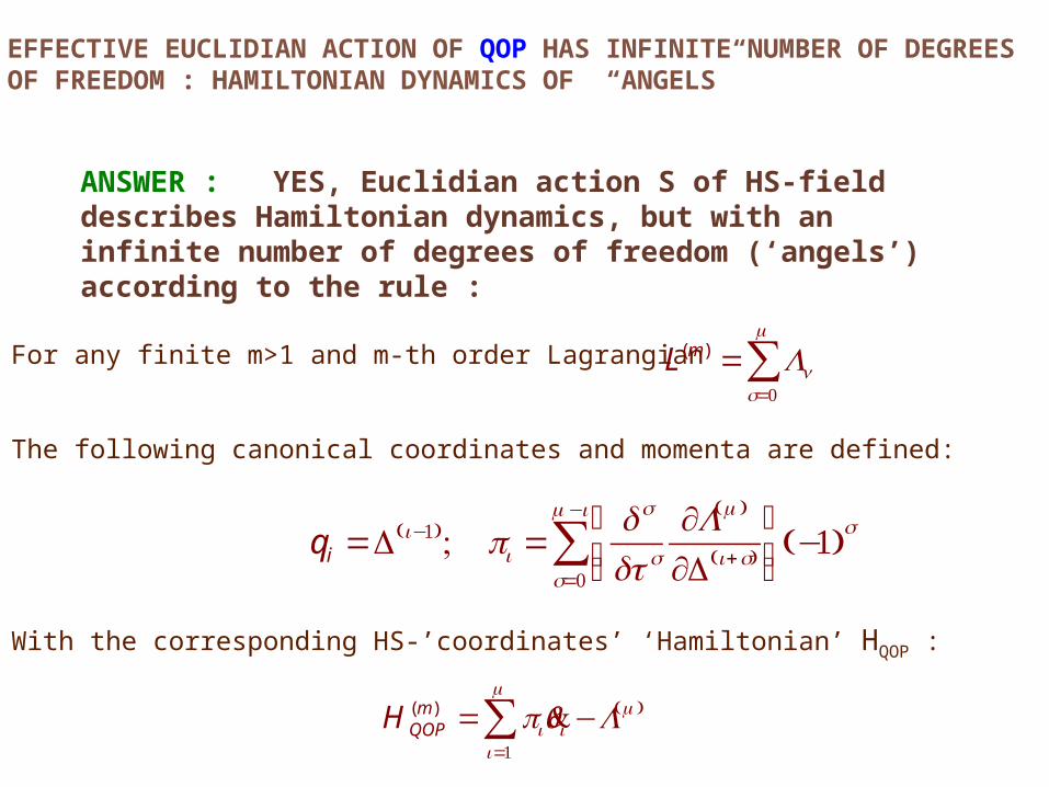
EFFECTIVE EUCLIDIAN ACTION OF QOP HAS INFINITE NUMBER OF DEGREESOF FREEDOM : HAMILTONIAN DYNAMICS OF “ANGELS”

ANSWER : YES, Euclidian action S of HS-field describes Hamiltonian dynamics, but with an infinite number of degrees of freedom (‘angels’) according to the rule :

qi =Δ(i−1); pi =ds

dτ s

∂L(m)

∂Δ(i+s)

⎛

⎝⎜⎞

⎠⎟s=0

m−i

∑ −1( )s

For any finite m>1 and m-th order Lagrangian

The following canonical coordinates and momenta are defined:

With the corresponding HS-’coordinates’ ‘Hamiltonian’ НQOP :

L(m ) = Lns=0

m

∑

H (m )

QOP = pii=1

m

∑ &qi −L(m)

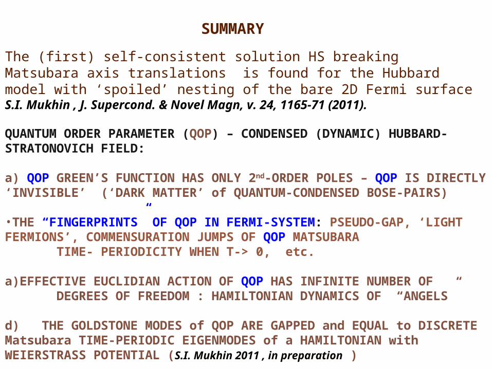
SUMMARY

The (first) self-consistent solution HS breaking Matsubara axis translations is found for the Hubbard model with ‘spoiled’ nesting of the bare 2D Fermi surface S.I. Mukhin , J. Supercond. & Novel Magn, v. 24, 1165-71 (2011).

QUANTUM ORDER PARAMETER (QOP) – CONDENSED (DYNAMIC) HUBBARD-STRATONOVICH FIELD:

a) QOP GREEN’S FUNCTION HAS ONLY 2nd-ORDER POLES – QOP IS DIRECTLY ‘INVISIBLE’ (‘DARK MATTER’ of QUANTUM-CONDENSED BOSE-PAIRS)

•THE “FINGERPRINTS” OF QOP IN FERMI-SYSTEM: PSEUDO-GAP, ‘LIGHT FERMIONS’, COMMENSURATION JUMPS OF QOP MATSUBARA TIME- PERIODICITY WHEN T-> 0, etc.

a)EFFECTIVE EUCLIDIAN ACTION OF QOP HAS INFINITE NUMBER OF DEGREES OF FREEDOM : HAMILTONIAN DYNAMICS OF “ANGELS”

d) THE GOLDSTONE MODES of QOP ARE GAPPED and EQUAL to DISCRETE Matsubara TIME-PERIODIC EIGENMODES of a HAMILTONIAN with WEIERSTRASS POTENTIAL (S.I. Mukhin 2011 , in preparation )

THANK YOU

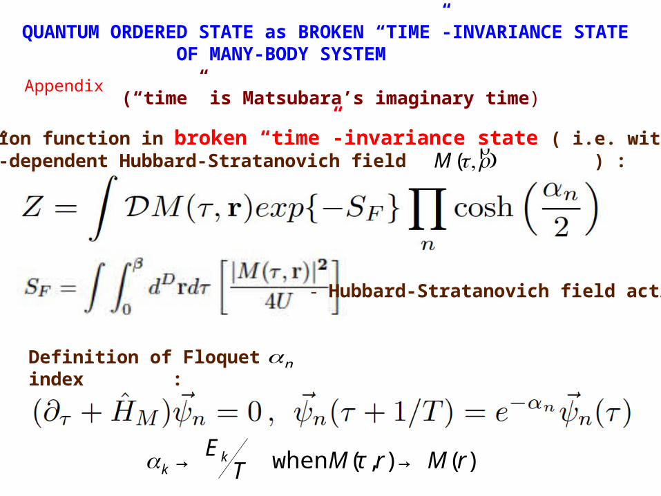
Partition function in broken “time”-invariance state ( i.e. with “time”-dependent Hubbard-Stratanovich field ) :

Definition of Floquet index :

€

αn

- Hubbard-Stratanovich field action

QUANTUM ORDERED STATE as BROKEN “TIME”-INVARIANCE STATE OF MANY-BODY SYSTEM

(“time” is Matsubara’s imaginary time)

€

αk → EkT when M(τ ,r) → M(r)

M (τ, rr )

Appendix

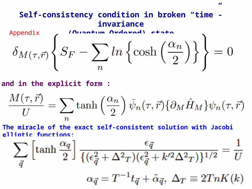
Self-consistency condition in broken “time”-invariance(Quantum Ordered) state

and in the explicit form :

The miracle of the exact self-consistent solution with Jacobi elliptic functions:

Appendix

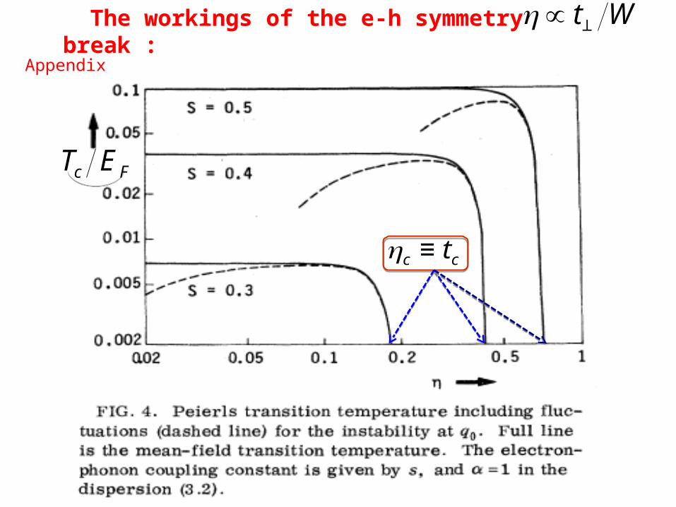
The workings of the e-h symmetry break :

(Horovitz, Gutfreund, Weger PRB (1975) )

€

Tc EF

€

η ∝ t⊥ W

€

ηc ≡ tc

Appendix

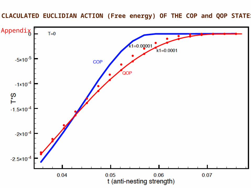
CLACULATED EUCLIDIAN ACTION (Free energy) OF THE COP and QOP STATES

Appendix

Appendix

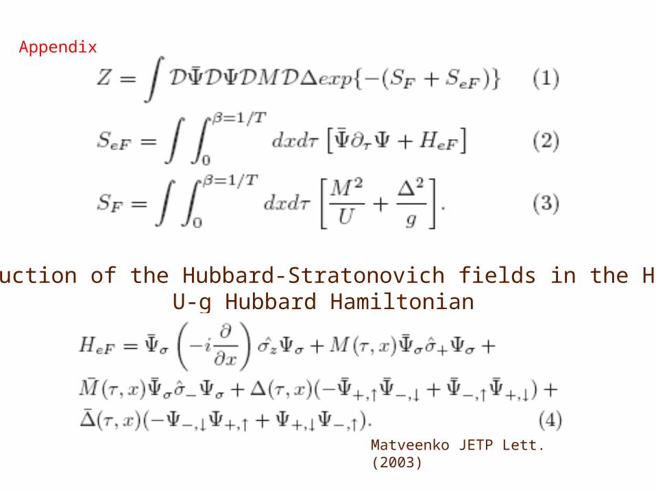
Introduction of the Hubbard-Stratonovich fields in the Hubbard U-g Hubbard Hamiltonian

Matveenko JETP Lett. (2003)

Appendix

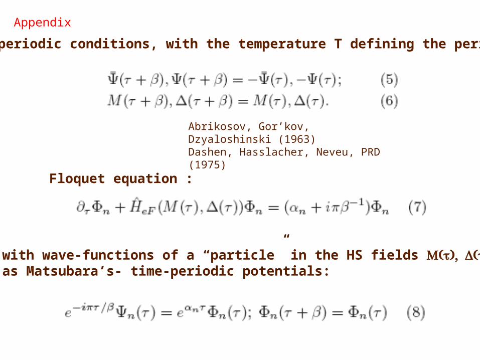
Abrikosov, Gor’kov, Dzyaloshinski (1963)Dashen, Hasslacher, Neveu, PRD (1975)

(anti)periodic conditions, with the temperature T defining the period β=T-1

Floquet equation :

with wave-functions of a “particle” in the HS fields τ Δτ as Matsubara’s- time-periodic potentials:

Appendix

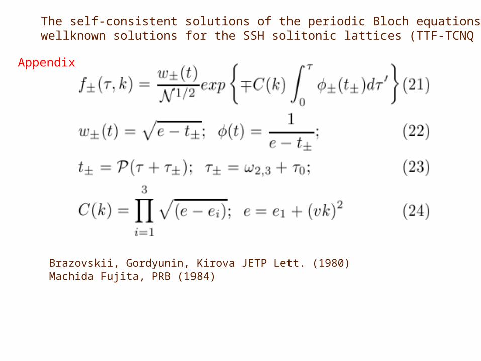
Brazovskii, Gordyunin, Kirova JETP Lett. (1980)Machida Fujita, PRB (1984)

The self-consistent solutions of the periodic Bloch equations are obtained using wellknown solutions for the SSH solitonic lattices (TTF-TCNQ theory):

Appendix

quantum order of fermions : broken matsubara time translations and quantum order fingerprints s.i....

Documents