quantum mechanics: notes - stargazinga classical mechanics of a point particle: review 67 b some...
TRANSCRIPT

Quantum Mechanics: Notes
Yi-Zen Chu
Contents
1 Basic Principles of Quantum Mechanics 2
2 Time Evolution in Quantum Mechanics 32.1 Properties of Evolution Operators . . . . . . . . . . . . . . . . . . . . . . . . . . 5
3 Heisenberg & Schrodinger Pictures:Time-Independent Hamiltonian 10
4 Interaction Picture 14
5 Poisson Brackets, Commutation Relations, & Momentum as the Generator ofTranslations 19
6 Non-Relativistic Quantum Mechanics 21
7 Hydrogen-like Atoms 227.1 Electric Dipole transitions . . . . . . . . . . . . . . . . . . . . . . . . . . . . . . 25
8 3D Rotation Symmetry in Quantum Systems 258.1 ‘Adding’ angular momentum . . . . . . . . . . . . . . . . . . . . . . . . . . . . . 288.2 Isospin symmetry . . . . . . . . . . . . . . . . . . . . . . . . . . . . . . . . . . . 31
9 Symmetry, Degeneracy & Conservation Laws 33
10 Spin and Statistics 3410.1 Spin Precession and Rotating Fermions . . . . . . . . . . . . . . . . . . . . . . . 3610.2 Atomic Structure/Periodic Table & Nuclear Structure . . . . . . . . . . . . . . . 37
11 Simple Harmonic Oscillator 3811.1 One Dimension . . . . . . . . . . . . . . . . . . . . . . . . . . . . . . . . . . . . 3811.2 Schrodinger vs Heisenberg . . . . . . . . . . . . . . . . . . . . . . . . . . . . . . 4311.3 Higher Dimensions . . . . . . . . . . . . . . . . . . . . . . . . . . . . . . . . . . 45
12 2-body Problem 48
1

13 Rigid Body Dynamics in 3D Space 4813.1 Classical . . . . . . . . . . . . . . . . . . . . . . . . . . . . . . . . . . . . . . . . 4813.2 Quantum . . . . . . . . . . . . . . . . . . . . . . . . . . . . . . . . . . . . . . . 52
14 Entanglement & Bell’s Inequalities: Spin-Half Systems; EPR Paradox 55
15 Path Integrals 5915.1 Example: Free Particle in Flat Euclidean Space . . . . . . . . . . . . . . . . . . 6115.2 Path Integrals From Time-Independent Hamiltonians . . . . . . . . . . . . . . . 64
15.2.1 General Properties . . . . . . . . . . . . . . . . . . . . . . . . . . . . . . 6915.2.2 Free Particle . . . . . . . . . . . . . . . . . . . . . . . . . . . . . . . . . . 7315.2.3 Simple Harmonic Oscillator . . . . . . . . . . . . . . . . . . . . . . . . . 73
16 Acknowledgments 81
A Classical Mechanics of a Point Particle: Review 81
B Some Identities 84
C Last update: March 31, 2020 84These notes on Quantum Mechanics currently follow no particular order. Please do feel free
to provide feedback, error reports, etc.
1 Basic Principles of Quantum Mechanics
Quantum Mechanics is the basic framework underlying the fundamental laws of Nature. Itsbasic principles are intimately tied to Linear Algebra.
Hilbert Space Given a physical system, its possible states are vectors in an abstractvector space, usually dubbed ‘Hilbert space’. This can be finite or infinite dimensional. Moreover,all information of the physical system are fully contained within the ket it corresponds to.
Observables as Hermitian Operators Many physical observables in quantum me-chanics – such as energy, position, momentum, spin, etc. – are described by Hermitian linearoperators. The possible outcomes of measuring these observables are the eigenvalues of theseHermitian operators.
To properly describe a quantum system usually means to find as many mutually commutingobservables as possible.
Born Rule Consider an observable A, with eigenstate |λ〉. When an experimentalisttries to measure A, the probability that the system described by |ψ〉 will be found in state |λ〉– and thereby yield λ as the observable – is given by
P (|ψ〉 → |λ〉) = |〈λ|ψ〉|2 (1.0.1)
provided both |ψ〉 and |λ〉 have been normalized to unit length.If λ refers to a continuous set of eigenvalues, then | 〈λ|ψ〉 |2 would instead be a probability
density – for example, | 〈~x|ψ〉 |2 is the probability per unit spatial volume for finding the quantumsystem at ~x, because |~x〉 is the position eigenstate infinitely sharply localized at ~x.
2

Because of this probabilistic interpretation of quantum mechanics, quantum states |ψ〉 arereally rays in a Hilbert space. If |ψ〉 describes the system at hand, the probability of finding itin the state |ψ〉 is unity by assumption. This only fixes its length-squared | 〈ψ|ψ〉 |2 = 1; thereis no other way to distinguish between eiδ |ψ〉 and |ψ〉, for real δ, and we are thus obliged toidentify all vectors differing only by an overall phase as corresponding to the same system.
Copenhagen The Copenhagen interpretation of quantum mechanics further states that,upon such a measurement, the original state |ψ〉 ‘collapses’ to |λ〉 if indeed the observable turnedout to be λ – at least for non-degenerate |λ〉. Suppose the system were degenerate, so that theeigen-subspace corresponding to the eigenvalue λ can be further labeled by say σ, we may denotethese states as |λ;σ〉. Now, if |ψ〉 is some superposition of these λ-states, namely
|λ′〉 ≡∑σ
Cσ |λ;σ〉 (Cσ ∈ C) (1.0.2)
plus other states with eigenvalues not equal to λ; then upon measuring A, if the experimentalistfinds λ, the state collapses instead to this |λ′〉:
|ψ〉 → |λ′〉√〈λ′|λ′〉
. (1.0.3)
Dynamics There is a ‘total energy’ operator, the Hamiltonian H, such that the time evo-lution of a state |ψ(t)〉 describing some physical system is governed by the Schrodinger equation:
i∂t |ψ(t)〉 = H |ψ(t)〉 , (1.0.4)
in units where ~ = 1.1 Physically speaking, quantum mechanics is really a framework; theactual physical content of a given quantum theory is encoded within its Hamiltonian. This isanalogous to Newton’s laws of mechanics; in particular, “force equals mass times acceleration”is the classical parallel to eq. (1.0.4) – the physics of Newton’s 2nd law is really specified by theactual form of the force law.
2 Time Evolution in Quantum Mechanics
Unitary Nature of Quantum Time Evolution In quantum mechanics, the physicalsystem is described by a state |ψ〉 in some Hilbert space. Suppose we identify some observableA. We know its eigenstates |λ〉 span the whole space, and therefore we may exploit thecompleteness relation I =
∑λ |λ〉 〈λ| to express
|ψ〉 =∑λ
|λ〉 〈λ|ψ〉 . (2.0.1)
The probability for finding the system a given state |λ′〉 is | 〈λ′|ψ〉 |2. On the other hand, theprobability to find it in any arbitrary state must be one, since these eigenstates span the whole
1Eq. (1.0.4) is the starting point for quantum dynamics. Often though – particularly in quantum field theory– one then quickly switches to the ‘Heisenberg picture’, where by choosing the analog of a rotating basis, thetime evolution is then transferred onto the operators.
3

space.
1 =∑λ
| 〈λ|ψ〉 |2 =∑λ
〈ψ|λ〉 〈λ|ψ〉 = 〈ψ|ψ〉 (2.0.2)
In other words, the state itself must have unit norm. Not only that, it must do so for all time.Otherwise, it would mean the probably of find it in any state is less than 1. (Where wouldit be, then?) As we see now the time evolution is unitary – probability is conserved – iff theHamiltonian is Hermitian.
The time-evolution equation carries Schrodinger’s name:
i∂t |ψ〉 = H |ψ〉 , (2.0.3)
−i∂t 〈ψ| = 〈ψ|H†. (2.0.4)
Consider now
∂t (〈ψ|ψ〉) = (∂t 〈ψ|) |ψ〉+ 〈ψ| (∂t |ψ〉) = i 〈ψ|H† |ψ〉 − i 〈ψ |H|ψ〉 (2.0.5)
= i 〈ψ|H† −H |ψ〉 . (2.0.6)
2If we want 〈ψ|ψ〉 = 1 to remain one for all time; its time derivative must be zero. Since thismust be true for any quantum state |ψ〉, we conclude
H = H†. (2.0.7)
On the other hand, if H = H† then the time derivative of 〈ψ|ψ〉 must be zero.Time Evolution Operator The time evolution operator U is the operator that obeys
the Schrodinger equation
i∂tU(t, t′) = HU(t, t′) (2.0.8)
and the boundary condition
U(t = t′) = I. (2.0.9)
Suppose we were given some state of a system at time t′, namely |ψ(t′)〉. Then the same physicalsystem at t > t′ can be gotten by acting U upon it:
|ψ(t)〉 = U(t, t′) |ψ(t′)〉 . (2.0.10)
That eq. (2.0.10) solves Schrodinger’s equation is because of eq. (2.0.8); while at t = t′, weutilize eq. (2.0.9) to check that |ψ(t)〉 → |ψ(t′)〉 is recovered.
Problem 2.1. Prove the following properties of the time-evolution operator:
U(t1, t2)U(t2, t3) = U(t1, t3) (2.0.11)
and
U(t1, t2)† = U(t2, t1); (2.0.12)
where t1,2,3 are arbitrary times.
2You might wonder why −i∂t 〈ψ| = 〈ψ|H†. Start with |ψ(t+ dt)〉 = |ψ(t)〉 − iHdt |ψ(t)〉+O((dt)2), which isequivalent to eq. (2.0.3). Then take the † on both sides to obtain 〈ψ(t+ dt)| = 〈ψ(t)|+ idt 〈ψ(t)|H† +O((dt)2);the ∂t 〈ψ| can be defined as the coefficient of dt.
4

Time-independent Hamiltonians & Stationary States Whenever the Hamiltoniandoes not depend on time, the time evolution operator is simply
U(t, t′) = exp (−iH(t− t′)) . (2.0.13)
It is easy to check that e−iH(t−t′) satisfies both equations eq. (2.0.8) and (2.0.9). Under thesecircumstances, if a quantum system is found in an energy eigenstate |En〉 at time t′, it willremain there for all times, since, according to eq. (2.0.10),
|ψ(t > t′)〉 = e−iH(t−t′) |En〉 = e−iEn(t−t′) |En〉 . (2.0.14)
2.1 Properties of Evolution Operators
In this section we will collect properties of evolution operators.Definition Given some initial/fixed time t′ and a Hermitian operator H – for our
purposes here in this section, it does not necessarily need to be the Hamiltonian – the definingequation of the evolution operator U is
i∂tU [t, t′] = H[t]U [t, t′], U [t = t′] = I. (2.1.1)
We shall assume H does not depend on time derivatives; in particular, since this is a first orderin time system, this means the solution to eq. (2.1.1) is unique. Taking the † on both sides alsohands us:
i∂tU†[t, t′] = −U †[t, t′]H[t], U †[t = t′] = I. (2.1.2)
Unitary The evolution operator defined by eq. (2.1.1) is unitary.Proof We wish to show that U †[t, t′]U [t, t′] = I. Using eq. (2.1.1), i.e., i∂tU = HU and
i∂tU† = −U †H, we see that the time evolution of the LHS is governed by:
i∂t(U †[t, t′]U [t, t′]
)= i∂tU
†[t, t′]U [t, t′] + U †[t, t′]i∂tU [t, t′] (2.1.3)
= −U †[t, t′]H[t]U [t, t′] + U †[t, t′]H[t]U [t, t′] = 0. (2.1.4)
Therefore, U †[t, t′]U [t, t′] is actually independent of t. To evaluate it for arbitrary t, therefore,we only need to do so at t = t′. The initial/boundary condition in eq. (2.1.1) says
U †[t = t′]U [t = t′] = I. (2.1.5)
Solution I The (unique) solution to eq. (2.1.1) is
U [t, t′] = I +∞∑`=1
(−i)`∫ t
t′dt`
∫ t`
t′dt`−1· · ·
∫ t3
t′dt2
∫ t2
t′dt1H[t`]H[t`−1] . . . H[t2]H[t1]. (2.1.6)
There is no restriction on whether t ≥ t′ or t < t′ here.
5

Proof The initial condition U [t = t′] = I is obeyed. Therefore, we need only to check thedifferential equation – i.e., Schrodinger’s equation – is satisfied:
i∂tU [t, t′] =∞∑`=1
(−i)`−1H[t]
∫ t
t′dt`−1
∫ t`−1
t′dt`−2· · ·
∫ t2
t′dt1H[t`−1] . . . H[t1]
= H[t]∞∑`=0
(−i)`∫ t
t′dt`
∫ t`
t′dt`−1· · ·
∫ t2
t′dt1H[t`] . . . H[t1]
= H[t]U [t, t′]
Note that the zeroth (` = 0) term of the sum on the second line is I.Solution II The (unique) solution to eq. (2.1.1) can also be written as
U [t, t′] = Θ 12[t− t′]T
exp
[−i∫ t
t′dt′′H[t′′]
]+ Θ 1
2[t′ − t]T
exp
[i
∫ t′
t
dt′′H[t′′]
], (2.1.7)
where T denotes time ordering, i.e., every operator within the . . . is to be arranged such thatoperators evaluated at later times sit to the left of operators evaluated at earlier times. Forexample,
TA[t1]B[t2] = Θ 12[t1 − t2]A[t1]B[t2] + Θ 1
2[t2 − t1]B[t2]A[t1],
and T denotes anti time ordering, i.e., every operator within the . . . is to be arranged suchthat operators evaluated at earlier times sit to the left of operators evaluated at later times. Forexample,
TA[t1]B[t2] = Θ 12[t2 − t1]A[t1]B[t2] + Θ 1
2[t1 − t2]B[t2]A[t1]. (2.1.8)
Here the step function is defined as
Θ 12[t− t′] = 1, if t > t′
Θ 12[t− t′] = 0, if t < t′
Θ 12[t− t′] =
1
2, if t = t′.
Also the (anti) time ordered exponential(s) in eq. (2.1.7) is formal – they are really defined byits Taylor expansion:
T
exp
[−i∫ t
t′dt′′H[t′′]
]≡ T
I +
∞∑`=1
(−i)`
`!
∫ t
t′dt`· · ·
∫ t
t′dt1H[t`] . . . H[t1]
, t ≥ t′,
(2.1.9)
and
T
exp
[i
∫ t′
t
dt′′H[t′′]
]≡ T
I +
∞∑`=1
i`
`!
∫ t′
t
dt`· · ·∫ t′
t
dt1H[t`] . . . H[t1]
, t < t′.
(2.1.10)
6
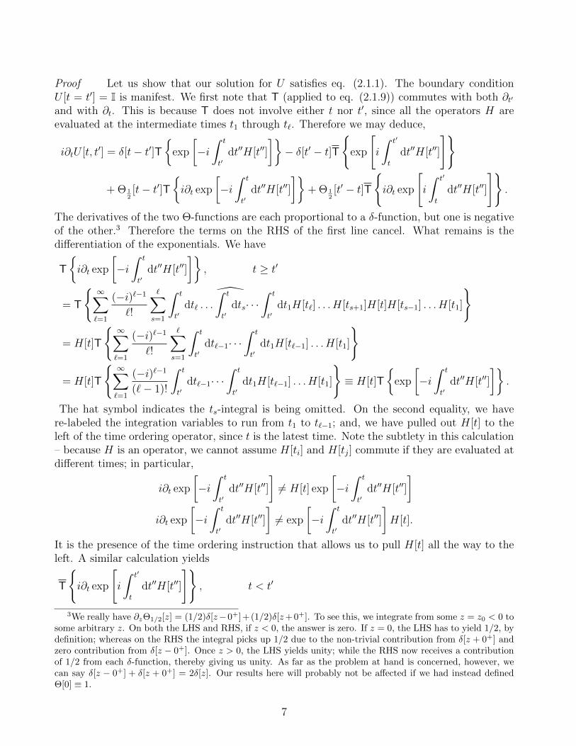
Proof Let us show that our solution for U satisfies eq. (2.1.1). The boundary conditionU [t = t′] = I is manifest. We first note that T (applied to eq. (2.1.9)) commutes with both ∂t′and with ∂t. This is because T does not involve either t nor t′, since all the operators H areevaluated at the intermediate times t1 through t`. Therefore we may deduce,
i∂tU [t, t′] = δ[t− t′]T
exp
[−i∫ t
t′dt′′H[t′′]
]− δ[t′ − t]T
exp
[i
∫ t′
t
dt′′H[t′′]
]
+ Θ 12[t− t′]T
i∂t exp
[−i∫ t
t′dt′′H[t′′]
]+ Θ 1
2[t′ − t]T
i∂t exp
[i
∫ t′
t
dt′′H[t′′]
].
The derivatives of the two Θ-functions are each proportional to a δ-function, but one is negativeof the other.3 Therefore the terms on the RHS of the first line cancel. What remains is thedifferentiation of the exponentials. We have
T
i∂t exp
[−i∫ t
t′dt′′H[t′′]
], t ≥ t′
= T
∞∑`=1
(−i)`−1
`!
∑s=1
∫ t
t′dt` . . .
∫ t
t′dts· · ·
∫ t
t′dt1H[t`] . . . H[ts+1]H[t]H[ts−1] . . . H[t1]
= H[t]T
∞∑`=1
(−i)`−1
`!
∑s=1
∫ t
t′dt`−1· · ·
∫ t
t′dt1H[t`−1] . . . H[t1]
= H[t]T
∞∑`=1
(−i)`−1
(`− 1)!
∫ t
t′dt`−1· · ·
∫ t
t′dt1H[t`−1] . . . H[t1]
≡ H[t]T
exp
[−i∫ t
t′dt′′H[t′′]
].
The hat symbol indicates the ts-integral is being omitted. On the second equality, we havere-labeled the integration variables to run from t1 to t`−1; and, we have pulled out H[t] to theleft of the time ordering operator, since t is the latest time. Note the subtlety in this calculation– because H is an operator, we cannot assume H[ti] and H[tj] commute if they are evaluated atdifferent times; in particular,
i∂t exp
[−i∫ t
t′dt′′H[t′′]
]6= H[t] exp
[−i∫ t
t′dt′′H[t′′]
]i∂t exp
[−i∫ t
t′dt′′H[t′′]
]6= exp
[−i∫ t
t′dt′′H[t′′]
]H[t].
It is the presence of the time ordering instruction that allows us to pull H[t] all the way to theleft. A similar calculation yields
T
i∂t exp
[i
∫ t′
t
dt′′H[t′′]
], t < t′
3We really have ∂zΘ1/2[z] = (1/2)δ[z−0+]+(1/2)δ[z+0+]. To see this, we integrate from some z = z0 < 0 tosome arbitrary z. On both the LHS and RHS, if z < 0, the answer is zero. If z = 0, the LHS has to yield 1/2, bydefinition; whereas on the RHS the integral picks up 1/2 due to the non-trivial contribution from δ[z + 0+] andzero contribution from δ[z − 0+]. Once z > 0, the LHS yields unity; while the RHS now receives a contributionof 1/2 from each δ-function, thereby giving us unity. As far as the problem at hand is concerned, however, wecan say δ[z − 0+] + δ[z + 0+] = 2δ[z]. Our results here will probably not be affected if we had instead definedΘ[0] ≡ 1.
7

= T
∞∑`=1
i`−1
`!
∑s=1
∫ t′
t
dt` . . .
∫ t′
t
dts· · ·∫ t′
t
dt1H[t`] . . . H[ts+1](−i2H[t])H[ts−1] . . . H[t1]
= H[t]T
∞∑`=1
i`−1
`!
∑s=1
∫ t′
t
dt`−1· · ·∫ t′
t
dt1H[t`−1] . . . H[t1]
= H[t]T
∞∑`=1
i`−1
(`− 1)!
∫ t′
t
dt`−1· · ·∫ t′
t
dt1H[t`−1] . . . H[t1]
≡ H[t]T
exp
[i
∫ t′
t
dt′′H[t′′]
].
This means we have proven our solution for U satisfies eq. (2.1.1).(Solution II)† We also have
U †[t, t′] = Θ 12[t− t′]T
exp
[i
∫ t
t′dt′′H[t′′]
]+ Θ 1
2[t′ − t]T
exp
[−i∫ t′
t
dt′′H[t′′]
], (2.1.11)
i.e.,
U †[t, t′] = U [t′, t]. (2.1.12)
Proof Simply take the Taylor series expansion in eq. (2.1.9) and take the † term by term.4
First, (−i)` is replaced with i` and vice versa. Second, for some arbitrary positive integer s, ifts > ts−1 > · · · > t2 > t1, then
(H[ts] . . . H[t1])† = H[t1] . . . H[ts].
That is, a time ordered product of operators become an anti time ordered product. Taking the †
on both sides once more shows an anti time ordered product of operators become a time orderedproduct.
Corollaries to Solution II The differential equation with respect to t′ is
i∂t′U [t, t′] = −U [t, t′]H[t′]. (2.1.13)
Therefore
i∂t′U†[t, t′] = H[t′]U †[t, t′]. (2.1.14)
Notice these equations with respect to t′ do not need to be imposed externally; they are aconsequence of the defining equations with respect to t (i.e., eq. (2.1.1)).
Proof Let us prove eq. (2.1.13) via a direct calculation. We have,
T
i∂t′ exp
[−i∫ t
t′dt′′H[t′′]
], t ≥ t′
= T
∞∑`=1
(−i)`−1
`!
∑s=1
∫ t
t′dt` . . .
∫ t
t′dts· · ·
∫ t
t′dt1H[t`] . . . H[ts+1](−H[t′])H[ts−1] . . . H[t1]
4Note: as long as the (anti) time ordered symbol is in place, the order of the operators within the . . . is
immaterial.
8

= −T
∞∑`=1
(−i)`−1
`!
∑s=1
∫ t
t′dt`−1· · ·
∫ t
t′dt1H[t`−1] . . . H[t1]
H[t′]
= −T
∞∑`=1
(−i)`−1
(`− 1)!
∫ t
t′dt`−1· · ·
∫ t
t′dt1H[t`−1] . . . H[t1]
H[t′] ≡ −T
exp
[−i∫ t
t′dt′′H[t′′]
]H[t′].
and
T
i∂t′ exp
[i
∫ t′
t
dt′′H[t′′]
], t < t′
= T
∞∑`=1
i`−1
`!
∑s=1
∫ t′
t
dt` . . .
∫ t′
t
dts· · ·∫ t′
t
dt1H[t`] . . . H[ts+1](i2H[t′])H[ts−1] . . . H[t1]
= −T
∞∑`=1
i`−1
`!
∑s=1
∫ t′
t
dt`−1· · ·∫ t′
t
dt1H[t`−1] . . . H[t1]
H[t′]
= −T
∞∑`=1
i`−1
(`− 1)!
∫ t′
t
dt`−1· · ·∫ t′
t
dt1H[t`−1] . . . H[t1]
H[t′] ≡ −T
exp
[i
∫ t′
t
dt′′H[t′′]
]H[t′].
A much simpler proof would be to start from the Schrodinger equation i∂tU [t, t′] = HU [t, t′],take the dagger on both sides, and employing eq. (2.1.12).
−i∂tU †[t, t′] = U †[t, t′]H, (2.1.15)
−i∂tU [t′, t] = U [t′, t]H. (2.1.16)
Group property The evolution operator obeys
U [t, t′′]U [t′′, t′] = U [t, t′], (2.1.17)
with no restriction on the relative chronologies of t, t′ and t′′.Proof We have to show that both sides obey the defining equations in eq. (2.1.1). It is
manifest that i∂tU = HU is obeyed and, as t → t′, the RHS tends to I. Thus, we merely haveto check the boundary condition that U [t, t′′]U [t′′, t′] tends to the identity when t→ t′: namely,U [t′, t′′]U [t′′, t′] = U †[t′′, t′]U [t′′, t′] = I, where eq. (2.1.12) was used in the first equality and theunitary property of U was employed in the second equality.
Operator insertion If we insert an operator Q in eq. (2.1.17):
U [t, t′]Q[t′]U [t′, t] = U †[t′, t]Q[t′]U [t′, t] = U [t, t′]Q[t′]U †[t, t′]
= Q[t′] +∞∑`=1
(−i)`∫ t
t′dt`
∫ t`
t′dt`−1· · ·
∫ t3
t′dt2
∫ t2
t′dt1
×[H[t`],
[H[t`−1],
[. . .[H[t2],
[H[t1], Q[t′]
]]. . .]]]
.
Proof As t → t′ we have the boundary condition U [t, t′]Q[t′]U [t′, t] → Q[t′]. This isobeyed on the RHS too. We may now check that both the LHS and RHS obeys the same first
9

order in time differential equation with respect to t. Differentiating LHS yields
i∂t(U [t, t′]Q[t′]U †[t, t′]
)= H[t]U [t, t′]Q[t′]U †[t, t′]− U [t, t′]Q[t′]U †[t, t′]H[t]
≡[H[t], U [t, t′]Q[t′]U †[t, t′]
].
Denote
R[t, t′] ≡ Q[t′] +∞∑`=1
(−i)`∫ t
t′dt`
∫ t`
t′dt`−1· · ·
∫ t3
t′dt2
∫ t2
t′dt1
[H[t`],
[H[t`−1],
[. . .[H[t1], Q[t′]
]. . .]]]
.
Differentiating the RHS gives us
i∂tR[t, t′] =∞∑`=1
(−i)`−1[H[t],
∫ t
t′dt`−1
∫ t`−1
t′dt`−2· · ·
∫ t3
t′dt2
∫ t2
t′dt1
[H[t`−1],
[. . .[H[t1], Q[t′]
]. . .]]]
=[H[t],R[t, t′]
]. (2.1.18)
3 Heisenberg & Schrodinger Pictures:
Time-Independent Hamiltonian
Just as choosing the right coordinates is often an important step in simplifying a given problem,the choice of the right basis in a given quantum mechanical problem can often provide thecrucial insights. Moreover, recall that the change-of-basis between two orthonormal basis isimplemented via a unitary transformation. In this section we will study the change-of-basisrelated to time-evolution itself, in the case where the Hamiltonian H is time-independent.
Schrodinger Picture If |ψ(t)〉 describes the physical state of a quantum system, theSchrodinger picture is defined as the basis where the Schrodinger equation is obeyed:
i∂t |ψ(t)〉 = H |ψ(t)〉 . (3.0.1)
If |ψ(t0)〉 is the state at time t0, you may verify through a direct calculation the solution to|ψ(t > t0)〉 is given by
|ψ(t ≥ t0)〉 = U(t, t0) |ψ(t0)〉 , (3.0.2)
U(t, t′) ≡ exp (−iH(t− t′)) , U(t = t′) = I. (3.0.3)
Eigen-spectrum Within the Schrodinger picture, the position, momentum and angular mo-mentum operators do not depend on time; and their eigenstates and values also do not dependon time. This statement also holds for any other time-independent observable A.
A |a〉 = a |a〉 : ∂t |a〉 = 0 if ∂tA = 0. (3.0.4)
If an observable A does not commute with the Hamiltonian H, then in general if a system attime t0 is found in one of its eigenstates |a〉, at a late time t > t0 it will no longer be the sameeigenstate. From eq. (3.0.2),
|ψ(t > t0)〉 = e−iH(t−t0) |a〉 (3.0.5)
10

is usually not proportional to |a〉 itself, for arbitrary |a〉, for it were then e−iH(t−t0) |a〉 = λa |a〉(for some eigenvalue λa) would be a simultaneous eigenket of both exp(−iH(t− t0)) and A andthus [H,A] = 0.
Heisenberg Picture The Heisenberg picture is usually defined using its relation to theSchrodinger picture. There is also a need to choose some time t0 where the two pictures coincide.
The motivation goes as follows, suppose |ψ(t)〉 is a physical state in the Schrodinger pictureand O is some (not necessarily Hermitian) time-independent operator. The time-dependentexpectation value of O with respect to this physical state is
〈ψ(t) |O|ψ(t)〉 . (3.0.6)
But using eq. (3.0.2),
〈ψ(t) |O|ψ(t)〉 =⟨ψ(t0)
∣∣U(t, t0)†OU(t, t0)∣∣ψ(t0)
⟩. (3.0.7)
Within the Heisenberg picture, physical states |ψ〉H are defined to be the ψ(t0) within theSchrodinger picture at time t0, namely
|ψ〉H ≡ |ψ(t0)〉 , (3.0.8)
and are therefore time-independent.Linear operators OH(t) in the Heisenberg picture are related to those in the Schrodinger
picture O through the change-of-basis implemented by the time evolution operator itself (cf.eq. (3.0.3)). Since U depends on time, this implies OH typically depends on time too:
OH(t) ≡ U(t, t0)†OU(t, t0). (3.0.9)
An exception occurs wheneverO commutes withH. For instance, wheneverH is time-independent,it commutes with itself for all times, and therefore
U †(t, t0)HU(t, t0) = e+iH(t−t0)He−iH(t−t0) = e+iH(t−t0)e−iH(t−t0)H = H. (3.0.10)
We highlight this important exception.
Whenever the Hamiltonian H is time independent, it takes the same form in boththe Heisenberg and Schrodinger pictures.
Returning to the defining Heisenberg picture equations (3.0.8) and (3.0.9), we see that eq. (3.0.7)may now be written as
〈ψ(t) |O|ψ(t)〉 = H 〈ψ |OH(t)|ψ〉H . (3.0.11)
Eigen-spectrum Within the Heisenberg picture, eq. (3.0.9) tells us that observables are
generically time-dependent. For example, whenever the position ~X, momentum ~P , and/or
angular momentum operators ~J do not commute with the Hamiltonian H, they become time-dependent in the Heisenberg picture.
~XH(t) = U(t, t0)† ~XU(t, t0), (3.0.12)
~PH(t) = U(t, t0)† ~PU(t, t0), (3.0.13)
~JH(t) = U(t, t0)† ~JU(t, t0). (3.0.14)
11

This in turn implies, since observables A are generically time-dependent, their eigen-statesbecome generically time dependent too:
AH(t) |a, t〉H = a |a, t〉H . (3.0.15)
Problem 3.1. Equations-of-Motion Whenever O does not commute with H, then com-puting U †OU may not be easy.5 An alternate perspective is to tackle the following first orderequation. Prove that
OH(t) = i [H,OH(t)] . (3.0.16)
If ~XH, ~PH and ~JH are the position, momentum and orbitary angular momentum operators of thesimple harmonic oscillator with Hamiltonian
H =1
2~P 2 +
ω2
2~X2, (3.0.17)
solve them in terms of their Schrodinger counterparts ~X, ~P and ~J .
Ehrenfest Theorem Suppose the Hamiltonian is the usual kinetic plus potential energy,namely
H =~P 2
2m+ V ( ~X). (3.0.18)
We will now see that Newton’s second law is recovered at the operator level, namely
m ~XH = −~∇V ( ~XH). (3.0.19)
To see this, we simply employ eq. (3.0.16) and[X i
(s), P(s)j
]= iδij ⇔ U(t, t0)†
[X i
(s), P(s)j
]U(t, t0) =
[X i
(H), P(H)j
]= iδij. (3.0.20)
Suppressing the subscript H, but working in the Heisenberg picture – the second derivative reads
X i = i[H, X i
]= i2
[H,[H,X i
]]= −
[~P 2
2m+ V,
[~P 2
2m,X i
]]= −(2m)−1
[~P 2
2m+ V, Pj
[Pj, X
i]
+[Pj, X
i]Pj
]= im−1
[V ( ~X), Pi
]= −m−1~∇V ( ~X). (3.0.21)
Problem 3.2. Anti-Time-Evolution If at arbitrary time t, the |a, t〉H is an eigenstate ofthe observable AH(t), show that
|a, t〉H = U(t, t0)† |a〉 . (3.0.22)
Namely, eigenkets in the Heisenberg picture are the anti-time-evolved Schrodinger picture ones.Explain why the eigenvalues do not depend on time, as long as the operator A in the Schrodingerpicture is time-independent.
5One may always write down an infinite series expansion using the Baker-Campbell-Hausdorff lemma.
12

The completeness relation of observables A in the Schrodinger picture reads∑a
|a〉 〈a| = I, A |a〉 = a |a〉 . (3.0.23)
In the Heisenberg picture, they read∑a
|a, t〉H H 〈a, t| = I, AH(t) |a, t〉H = a |a, t〉H . (3.0.24)
For instance, if ~X is the position operator and ~x is its eigenket,∫dD~x |~x, t〉H H 〈~x, t| = I. (3.0.25)
To demonstrate the validity of eq. (3.0.24), we employ eq. (3.0.22) followed by the completenessrelation in the Schrodinger picture.∑
a
|a, t〉H H 〈a, t| = U(t, t0)†∑a
|a〉 〈a|U(t, t0) = U(t, t0)†IU(t, t0) = I. (3.0.26)
Of course, we could also simply recognize eq. (3.0.9), with O = A here, as being a change-of-basis, which does not affect the Hermitian character of the operator in question.
Problem 3.3. Show that
H 〈~x, t| a, t〉H = 〈~x| a〉 . (3.0.27)
That is, the position-representation of some eigenket of an observable is picture-independent.
Problem 3.4. Energy Eigenket Expectation Value Explain why
〈E |O|E〉 = H 〈E, t? |OH(t)|E, t?〉H , (3.0.28)
where t? is an arbitrary time. In the Schrodinger picture, recall that, if the physical system isin the energy eigenstate |ψ(t0)〉 = |E〉, then 〈ψ(t) |O|ψ(t)〉 = 〈E |O|E〉; i.e., the time t in |ψ(t)〉is immaterial. This result in eq. (3.0.28) tells us the same statement holds in the Heisenbergpicture.
13

4 Interaction Picture
Motivation In many situations, the Hamiltonian H is the sum of an exactly solvable (or,at least, well understood) H0 and a complicated but ‘small’ perturbation H ′.
H = H0 +H ′ (4.0.1)
For instance, H0 might describe the hydrogen atom and H ′ its interaction with an externallyapplied electromagnetic field. We shall see how the interaction picture allows us to re-writeSchrodinger’s equation in such a way to implement perturbation theory in powers of H ′.
Time Evolution We will define the interaction picture in terms of the Schrodingerpicture. Denoting the former by the subscript ‘I’ and the latter by ‘s’, physical states are relatedvia
|ψ(t)〉I = U †0 |ψ(t)〉s , (4.0.2)
where U0 is the time evolution operator corresponding to H0, namely
i∂tU0(t, t0) = H0U0(t, t0) and U0(t = t0) = I. (4.0.3)
Referring to eq. (4.0.2), the t0 is therefore the time where the Schrodinger and interactionpictures coincide.
The linear operators are related via
OI = U †0OsU0. (4.0.4)
This is to preserve the form of the matrix element between arbitrary states |ψ1,2〉:
I 〈ψ1(t) |OI|ψ2(t)〉I = s
⟨ψ1(t)
∣∣∣U0U†0OsU0U
†0
∣∣∣ψ2(t)⟩
s(4.0.5)
= s 〈ψ1(t) |Os|ψ2(t)〉s . (4.0.6)
The eigenkets |a; t〉I of an observable AI within the interaction picture are related to itsSchrodinger picture counterparts |a; t〉s of an observable As through
|a; t〉I = U0(t, t0)† |a〉s ; (4.0.7)
because
AI |a; t〉I = U †0AsU0U†0 |a〉s (4.0.8)
= U †0As |a〉s = a · U †0 |a〉s (4.0.9)
= a |a; t〉I . (4.0.10)
Let us examine the time evolution of an interaction picture state. If, within the Schrodingerpicture,
i∂tU(t, t′) = HU(t, t′) = (H0 +H ′)U(t, t′) and U(t = t′) = I; (4.0.11)
14

then according to eq. (4.0.2),
|ψ(t)〉I = UI(t, t0) |ψ(t0)〉s , (4.0.12)
UI(t, t0) ≡ U0(t, t0)†U(t, t0). (4.0.13)
This UI is not the Schrodinger picture U re-expressed in interaction picture,6 but we are abusingnotation somewhat for technical convenience. In any case, UI does take a Schrodinger pictureinitial state and evolves it to an interaction picture state at time t. What is important is itsequations-of-motion.
iUI = −(iU0)†U + U0(iU) (4.0.14)
= U †0(−H0)U + U0HU (4.0.15)
= U †0(−H0 +H0 +H ′)U = U †0H′U0U
†0U (4.0.16)
= H ′IUI. (4.0.17)
In words: the UI obeys the Schrodinger equation, but with respect to the Hamiltonian H ′I writtenin the interaction picture.
Operator Equation Admitting Dyson Series As Solution Consider the operatorequation
A = BA, (4.0.18)
where the overdot denotes time derivative, and both A and B are operators. The solution is theDyson series
A(t) =
(I +
+∞∑`=1
∫ t
t0
ds`
∫ s`
t0
ds`−1· · ·∫ s3
t0
ds2
∫ s2
t0
ds1B(s`)B(s`−1) . . . B(s2)B(s1)
)A(t0).
(4.0.19)
Note that the ordering of these Bs and A(t0) are important, because they are operators. Fromeq. (4.0.14) and the initial condition UI(t = t0) = I, we may therefore solve the UI solely interms of H ′I.
UI(t, t0) =
(I +
+∞∑`=1
(−i)`∫ t
t0
ds`
∫ s`
t0
ds`−1· · ·∫ s3
t0
ds2
∫ s2
t0
ds1H′I(s`)H
′I(s`−1) . . . H ′I(s2)H ′I(s1)
).
(4.0.20)
Time-Dependent Perturbation Theory As an application of the interaction pictureformalism, let us now examine the following problem. We will assume H0 is a time-independentHermitian operator; whereas H ′ is a time-dependent one. As we shall witness, the interactionpicture physical ket may therefore be solved in terms of the eigenkets of H0, which obey
H0
∣∣En⟩s= En
∣∣En⟩s. (4.0.21)
6The interaction picture evolution operator, namely U†0 (t, t0)U(t, t0)U0(t, t0), does not in fact evolve the
initial state properly – i.e., |ψ(t)〉I 6= U†0 (t, t0)U(t, t0)U0(t, t0) |ψ(t0)〉I – because the state it acts on (namely,
|ψ(t0)〉I = |ψ(t0)〉s) is not evaluated at the same time as the operator itself.
15

From eq. (4.0.7) and the time-independence of the H0 to recall U0(t, t0) = exp(−iH0(t− t0)),∣∣En; t⟩
I= eiEn(t−t0)
∣∣En⟩s. (4.0.22)
The solution, according to eq. (4.0.20) inserted into eq. (4.0.12), is
|ψ(t)〉I (4.0.23)
=
(I +
+∞∑`=1
(−i)`∫ t
t0
ds`
∫ s`
t0
ds`−1· · ·∫ s3
t0
ds2
∫ s2
t0
ds1H′I(s`)H
′I(s`−1) . . . H ′I(s2)H ′I(s1)
)|ψ(t0)〉 .
Employing eq. (4.0.7)
U0 |a; t〉I = |a〉s and I 〈a; t| = s 〈a|U0; (4.0.24)
as well as |ψ(t)〉s = U(t, t0) |ψ(t0)〉, the quantum amplitude for finding the physical system inthe eigenstate
∣∣En⟩ at time t is given by
s
⟨En∣∣ψ(t)
⟩s
= I
⟨En; t
∣∣U0(t, t0)†U(t, t0)∣∣ψ(t0)
⟩(4.0.25)
= I
⟨En; t |UI(t, t0)|ψ(t0)
⟩= I
⟨En; t
∣∣ψ(t)⟩
I. (4.0.26)
First Order Time-Dependent PT To first order in H ′I, we may employ eq. (4.0.23) todeduce the quantum transition amplitude is
s
⟨En∣∣ψ(t)
⟩s
= I
⟨En; t
∣∣ψ(t)⟩
I(4.0.27)
= I
⟨En; t
∣∣ I− i ∫ t
t0
H ′I(s)ds+ . . . |ψ(t0)〉 (4.0.28)
In particular, if the physical system began at some eigenstate of H0, say
|ψ(t0)〉 =∣∣Ea⟩s
; (4.0.29)
then we see that the transition amplitude M(Ea → ~Eb) is provided by the expression
M(Ea → ~Eb) ≡ s
⟨En∣∣ψ(t)
⟩s
= I
⟨En; t
∣∣ψ(t)⟩
I(4.0.30)
= e−iEb(t−t0)
(δba − i
∫ t
t0
s
⟨Eb
∣∣∣U †0H ′s(s)U0
∣∣∣ Ea⟩s+ . . .
)(4.0.31)
= e−iEb(t−t0)
(δba − i
∫ t
t0
ei(Eb−Ea)(s−t0)s
⟨Eb |H ′s(s)| Ea
⟩s+ . . .
)(4.0.32)
If, furthermore, we are interested in nontrivial transitions (b 6= a); then the probability of sucha process is – up to first order in perturbation theory – given by∣∣∣M(
Ea → ~Eb;b6=at0→t
)∣∣∣2 ≈ ∣∣∣∣∫ t
t0
ei(Eb−Ea)ss
⟨Eb |H ′s(s)| Ea
⟩s
∣∣∣∣2 . (4.0.33)
16

Harmonic Perturbation & Fermi’s Golden Rule Consider a perturbation that is purelyharmonic, with positive frequency (ω > 0),
H ′(t) = −V0e−iωt − V †0 e+iωt. (4.0.34)
Here, V0 is an arbitrary but constant perturbation, whose eigenvalues we will assume are muchsmaller than those of H0.
For simplicity, let us now consider the case where the system began at some energy eigenstate∣∣Ea⟩ an infinitely long time ago, i.e., t0 → −∞; while the observation is made an infinitely longtime in the future, i.e., t→ +∞. Eq. (4.0.33) reads∣∣∣M(
Ea → ~Eb;b 6=at0→t
)∣∣∣2 (4.0.35)
≈∣∣∣∣∫
Rei(Eb−Ea)s
s
⟨Eb
∣∣∣V0e−iωs + V †0 e
+iωs∣∣∣ Ea⟩
s
∣∣∣∣2=∣∣∣ s
⟨Eb
∣∣∣V0(2π)δ(Ea − Eb + ω
)+ V †0 (2π)δ
(Ea − Eb − ω
)∣∣∣ Ea⟩s
∣∣∣2=∣∣(2π)δ
(Ea + ω − Eb
)s
⟨Eb |V0| Ea
⟩s
∣∣2 +∣∣∣(2π)δ
(Ea − ω − Eb
)s
⟨Eb
∣∣∣V †0 ∣∣∣ Ea⟩s
∣∣∣2 .In the last line, there are no cross terms, which would otherwise contain δ(Ea − Eb − ω)δ(Ea −Eb +ω), because it is not possible for the arguments to be simultaneously equal to zero; namely
Ea − Eb = ω = −ω (4.0.36)
cannot be true unless ω = 0. In fact, the two Dirac δ-functions correspond to
• Ea − ω = Eb: (Absorption) Ending up with a lower energy indicates an externalquanta of energy ω was absorbed.
• Ea+ω = Eb: (Emission) Ending up with a higher energy indicates an external quantaof energy ω was emitted.
Now, there is a mathematical issue with the last equality of eq. (4.0.35). It contains terms like((2π)δ
(Ea − Eb − ω
))2= (2π)δ
(Ea − Eb − ω
)· (2π)δ (0) and (4.0.37)(
(2π)δ(Ea − Eb + ω
))2= (2π)δ
(Ea − Eb + ω
)· (2π)δ (0) . (4.0.38)
The interpretation of the 2πδ(0) is as follows
((2π)δ
(Ea − Eb − ω
))2= (2π)δ
(Ea − Eb − ω
) ∫Rei(Ea−Eb−ω)sds (4.0.39)
= (2π)δ(Ea − Eb − ω
)limT→∞
∫ +T
−Tds (4.0.40)
= (2π)δ(Ea − Eb − ω
)· (∞-time duration); (4.0.41)
17

Dividing eq. (4.0.35) throughout by (2π)δ(0) then allows us to re-interpret the result as the rateper unit time of transitioning from Ea to Eb. This result is the celebrated Fermi’s Golden Rule:
Number of Ea → Eb transitions, with b 6= a
Total time≡
∣∣∣M(Ea → ~Eb;
b6=at0→t
)∣∣∣22πδ(0)
(4.0.42)
= (2π)δ(Ea − Eb − ω
) ∣∣s
⟨Eb |V0| Ea
⟩s
∣∣2 + (2π)δ(Ea − Eb + ω
) ∣∣∣ s
⟨Eb
∣∣∣V †0 ∣∣∣ Ea⟩s
∣∣∣2 . (4.0.43)
Rant I consider this derivation to be rather sloppy. Why should one expect first order PTto remain valid over an infinite time period? The original calculation for |M|2 is a probability– why are we allowed to re-interpret its infinite time limit as a transition rate (i.e., number oftransitions per unit time)? Unfortunately, most textbooks do not justify Fermi’s Golden Rulevery well; my lack of rigor may only be justified – rather unscientifically! – by blaming others:everyone else does (roughly) the same thing!Relation to Weinberg’s Discussion [1] Weinberg’s §6 stayed within the Schrodinger picture.
|ψ(t)〉s =∑n
∣∣En⟩s s
⟨En∣∣ψ(t)
⟩s
(4.0.44)
=∑n
∣∣En⟩s I
⟨En; t
∣∣ψ(t)⟩
I. (4.0.45)
Referring to equations (4.0.24) and (4.0.25), we see that
|ψ(t)〉s =∑n
e−iEn(t−t0)∣∣En⟩s s
⟨En |UI(t, t0)|ψ(t0)
⟩. (4.0.46)
Comparison with Weinberg’s eq. (6.1.4) reveals the identifications
En ↔ En(Weinberg) (4.0.47)
eiEat0∣∣Ea⟩s
↔ Ψn(Weinberg) (4.0.48)
s
⟨En |UI(t, t0)|ψ(t0)
⟩↔ cn(Weinberg). (4.0.49)
Problem 4.1. Show that this identification is consistent with Weinberg’s equation (6.1.5); i.e.,show that s
⟨En |UI(t, t0)|ψ(t0)
⟩obeys the same differential equation as Weinberg’s cn(t). Hint:
Remember that UI obeys the Schrodinger equation with respect to the perturbation H ′I, but inthe interaction picture.
18

5 Poisson Brackets, Commutation Relations, & Momen-
tum as the Generator of Translations
Consider an infinite D−dimensional flat space. In the Hilbert space spanned by the eigenkets|~x〉 of the position operator ~X, the translation operator is unitary and may be written as
T (~d) =
∫RD
dD~x∣∣∣~x+ ~d
⟩〈~x| (5.0.1)
= exp(−i~d · ~P
). (5.0.2)
Because T is unitary, the ‘momentum’ ~P is Hermitian. Strictly speaking, ~P is of dimensions1/[Length] – i.e., it is not really momentum. To produce an operator that is in fact of dimension[momentum] = [angular momentum]/[length], we need to multiply a dimensionful quantity κ to~P such that
[κ][~P ] = [momentum]. (5.0.3)
Because [~P ] = 1/[Length], we must have
[κ] = [angular momentum]. (5.0.4)
In Quantum Mechanics, this constant is nothing but ~:
~~P ≡ momentum. (5.0.5)
Why we would choose to do something like that, has to do with the analogy between the Poissonbrackets of classical mechanics and the commutator of quantum mechanics.Poisson bracket From §(A), we see that the generator of spatial translation in classicalmechanics is the momentum pi, in that
f (~q, ~p) , piPB =∂f
∂qi. (5.0.6)
The generator of time translation is the Hamilton H, in that
f (~q(t), ~p(t)) , HPB =d
dtf (~q(t), ~p(t)) . (5.0.7)
Quantum Dynamics In the Heisenberg picture, and assuming the Hamiltonian H is time-independent, an operator OH obeys the first order in time ODE:
OH =1
i~[OH, H] . (5.0.8)
Linear algebra |~x〉 If we assume that, for an arbitrary ket |ψ〉,
〈~x| f(~X, ~P
)|ψ〉 = f
(~x,−i~∇
)〈~x|ψ〉 . (5.0.9)
19

This amounts to assuming a certain operator ordering. For example, this would pan out if allthe position operators stand to the left and the momentum to the right; for e.g.,⟨
~x∣∣∣ ~X2 ~P 2
∣∣∣ψ⟩ = ~x2(−i)2∂i∂i 〈~x|ψ〉 . (5.0.10)
Let us now consider⟨~x∣∣∣[f ( ~X, ~P) , Pj]∣∣∣ψ⟩ = f
(~x,−i~∇
)〈~x |Pj|ψ〉 − (−)i~∇
⟨~x∣∣∣f ( ~X, ~P)∣∣∣ψ⟩ (5.0.11)
= −if(~x,−i~∇
)∂j 〈~x|ψ〉+ i~∇
(f(~X, ~P
)〈~x|ψ〉
)(5.0.12)
= i(~∇f(~X, ~P
))〈~x|ψ〉 . (5.0.13)
In other words, since |ψ〉 was arbitrary,
∂f(~X, ~P
)∂Xj
=1
i
[f(~X, ~P
), Pj
]. (5.0.14)
Notice there is a ~ in eq. (5.0.8) (I’ve deliberately restored it); but none in eq. (5.0.14).Comparison Identifying eq. (5.0.7) with eq. (5.0.8) (as well as f ↔ OH); and eq.
(5.0.6) with eq. (5.0.14) – we now see the following classical-quantum correspondence.
• The Poisson bracket ·, ·PB in classical mechanics should be identified with the commu-tator (i~)−1[·, ·] of quantum mechanics.
• The Hamiltonian in classical mechanics should be identified with the Hamiltonian in quan-tum mechanics.
• The momentum in classical mechanics ~P should be identified with the −i~~∇ in quantummechanics (within the position representation).
20

6 Non-Relativistic Quantum Mechanics
Total Energy From the previous section, we see that the momentum operator in QM isto be identified with the generator of translations in the following manner:
〈~x| ~P |ψ〉 = −i~~∇ 〈~x|ψ〉 . (6.0.1)
That, in turn, means that the square of the momentum is the (negative) Laplacian:
〈~x| ~P 2 |ψ〉 = −~2~∇2 〈~x|ψ〉 . (6.0.2)
Within the Hamiltonian formalism, the classical Hamiltonian H itself is usually kinetic pluspotential energy V (i.e., total energy). In the previous section, we have also identified the QM
Hamilton with the classical one. Since kinetic energy is ~P 2/(2m), we may therefore identify, innon-relativistic QM:
〈~x|H |ψ〉 = 〈~x|
(~P 2
2m+ V ( ~X)
)|ψ〉 (6.0.3)
=
(− ~2
2m~∇2 + V (~x)
)〈~x|ψ〉 . (6.0.4)
Schrodinger ’s equation (2.0.3) now takes the form:
i∂tψ(t, ~x) =
(− 1
2m~∇2 + V (~x)
)ψ(t, ~x), (6.0.5)
where ψ(t, ~x) ≡ 〈~x|ψ(t)〉 and ~ ≡ 1.Probability Current in NR QM In non-relativistic QM,
ρ ≡ |ψ(~x)|2 (6.0.6)
is the probability density of finding the particle at ~x. The associated (spatial) probability currentis
~J =i
2m
ψ~∇ψ∗ − ψ∗~∇ψ
. (6.0.7)
Altogether, they obey the conservation equation
∂ρ
∂t= −~∇ · ~J. (6.0.8)
This is perhaps best understood by integrating over some finite spatial volume D; applyingGauss’ theorem on the right hand side,
d
dt
∫D
ρ(t, ~x)dD~x = −∫∂D
~J(t, ~x) · dD−1~Σ. (6.0.9)
21

(The dD−1~Σ is the directed area element on the boundary of D, which I denote as ∂D.) Theinterpretation is, the rate of change of probability within D per unit time is accounted for bythe flux of the probability current through the boundary.
Let us turn to verifying eq. (6.0.8) using Schrodinger ’s equation (6.0.5).
ρ = (iψ)∗(iψ) + (iψ)∗(iψ) (6.0.10)
=(−(2m)−1~∇2 + V
)ψ∗ · (iψ)− iψ∗
(−(2m)−1~∇2 + V
)ψ (6.0.11)
= i(2m)−1(ψ∗~∇2ψ − ψ~∇2ψ∗
). (6.0.12)
On the other hand,
~∇ · ~J = i(2m)−1~∇ ·(ψ~∇ψ∗ − ψ∗~∇ψ
)(6.0.13)
= i(2m)−1(ψ~∇2ψ∗ − ψ∗~∇2ψ
)= −ρ. (6.0.14)
7 Hydrogen-like Atoms
The stationary-state Schrodinger equation describing an electron’s wavefunction ψ around aHydrogen-like atom is, in spherical coordinates (r, θ, φ),
〈~x |H|ψ〉 = E 〈~x|ψ〉 , (7.0.1)
− 1
2me
~∇2ψ − Ze2
rψ = − 1
2me
(1
r2∂r(r2∂rψ
)+
1
r2~∇S2ψ
)− Ze2
rψ = −Eψ. (7.0.2)
The first term on the left is the non-relativistic kinetic energy p2/(2me), where me is the electronmass. The −Ze2/r is the electric/Coulomb potential experienced by the electron orbiting arounda central nucleus with Z protons and e is the fundamental electric charge; and r the radius ofthe orbit. Moreover, we are going to be interested in bound states for now; so −E < 0.
We first perform a separation of variables,
ψ(r, θ, φ) = R(r)Y m` (θ, φ). (7.0.3)
Using the fact that Y m` is the eigenfunction of the Laplacian on the unit sphere, with eigenvalue
−`(`+ 1),
~∇S2Ym` = −`(`+ 1)Y m
` , (7.0.4)
we have
−R′′(r)
2me
− R′(r)
mer+
(E +
`(`+ 1)
2mer2− Z · e2
r
)R(r) = 0. (7.0.5)
Next, we re-scale
ρ ≡√
2meEr, ξ ≡√
2me
Ee2Z; (7.0.6)
22

to obtain
−R′′(ρ)− 2
ρR′(ρ) +
(1− ξ
ρ+`(`+ 1)
ρ2
)R(ρ) = 0. (7.0.7)
Next, we apply the ansatz
R(ρ) = ρ` exp(−ρ)F (ρ) (7.0.8)
to convert the above ODE into
F ′′(ρ) + 2
(`+ 1
ρ− 1
)F ′(ρ) +
ξ − 2`− 2
ρF (ρ) = 0. (7.0.9)
Let’s solve it via a power series
F (ρ) =+∞∑s=0
asρs. (7.0.10)
One would find that
+∞∑s=0
((s− 1)sasρ
s−2 + asρs−1(ξ − 2`− 2)− 2sasρ
s−1 + 2sasρs−2(`+ 1)
)= 0. (7.0.11)
The only s = 0 term is
s = 0 : a0(ξ − 2`− 2)ρ−1. (7.0.12)
By replacing s→ s+1 in the ρs−2 terms, we see that, for s ≥ 1, requiring that each independentpower of ρ to vanish implies
(2(1 + s+ `)− ξ)as = (1 + s)(s+ 2`+ 2)as+1. (7.0.13)
Following Weinberg [1] we make the following asymptotic argument. For large s, notice
as+1 =2(1 + s+ `)− ξ
(1 + s)(s+ 2`+ 2)as →
2
sas. (7.0.14)
As Weinberg argues, since as+1 and as have the same sign for large s, the infinite series isdominated by these large s terms as ρ→∞. Therefore we may approximate
as ≈2
sas−1 ≈
22
s(s− 1)as−2 ≈
2s
s!a0. (7.0.15)
Of course, once s is small enough, as+1/as is no longer 2/s; Weinberg asserts that one shouldinstead write
as ≈2s
(s+B)!C, (7.0.16)
23
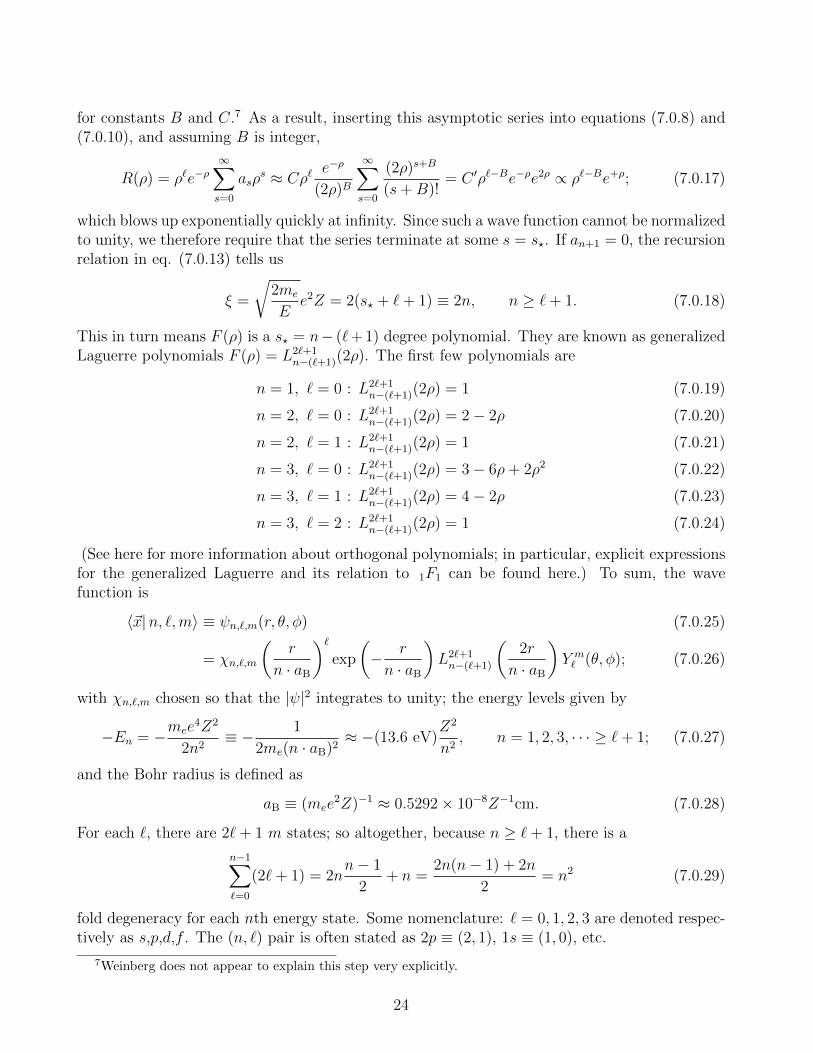
for constants B and C.7 As a result, inserting this asymptotic series into equations (7.0.8) and(7.0.10), and assuming B is integer,
R(ρ) = ρ`e−ρ∞∑s=0
asρs ≈ Cρ`
e−ρ
(2ρ)B
∞∑s=0
(2ρ)s+B
(s+B)!= C ′ρ`−Be−ρe2ρ ∝ ρ`−Be+ρ; (7.0.17)
which blows up exponentially quickly at infinity. Since such a wave function cannot be normalizedto unity, we therefore require that the series terminate at some s = s?. If an+1 = 0, the recursionrelation in eq. (7.0.13) tells us
ξ =
√2me
Ee2Z = 2(s? + `+ 1) ≡ 2n, n ≥ `+ 1. (7.0.18)
This in turn means F (ρ) is a s? = n− (`+ 1) degree polynomial. They are known as generalizedLaguerre polynomials F (ρ) = L2`+1
n−(`+1)(2ρ). The first few polynomials are
n = 1, ` = 0 : L2`+1n−(`+1)(2ρ) = 1 (7.0.19)
n = 2, ` = 0 : L2`+1n−(`+1)(2ρ) = 2− 2ρ (7.0.20)
n = 2, ` = 1 : L2`+1n−(`+1)(2ρ) = 1 (7.0.21)
n = 3, ` = 0 : L2`+1n−(`+1)(2ρ) = 3− 6ρ+ 2ρ2 (7.0.22)
n = 3, ` = 1 : L2`+1n−(`+1)(2ρ) = 4− 2ρ (7.0.23)
n = 3, ` = 2 : L2`+1n−(`+1)(2ρ) = 1 (7.0.24)
(See here for more information about orthogonal polynomials; in particular, explicit expressionsfor the generalized Laguerre and its relation to 1F1 can be found here.) To sum, the wavefunction is
〈~x|n, `,m〉 ≡ ψn,`,m(r, θ, φ) (7.0.25)
= χn,`,m
(r
n · aB
)`exp
(− r
n · aB
)L2`+1n−(`+1)
(2r
n · aB
)Y m` (θ, φ); (7.0.26)
with χn,`,m chosen so that the |ψ|2 integrates to unity; the energy levels given by
−En = −mee4Z2
2n2≡ − 1
2me(n · aB)2≈ −(13.6 eV)
Z2
n2, n = 1, 2, 3, · · · ≥ `+ 1; (7.0.27)
and the Bohr radius is defined as
aB ≡ (mee2Z)−1 ≈ 0.5292× 10⁻⁸Z−1cm. (7.0.28)
For each `, there are 2`+ 1 m states; so altogether, because n ≥ `+ 1, there is a
n−1∑`=0
(2`+ 1) = 2nn− 1
2+ n =
2n(n− 1) + 2n
2= n2 (7.0.29)
fold degeneracy for each nth energy state. Some nomenclature: ` = 0, 1, 2, 3 are denoted respec-tively as s,p,d,f . The (n, `) pair is often stated as 2p ≡ (2, 1), 1s ≡ (1, 0), etc.
7Weinberg does not appear to explain this step very explicitly.
24

Problem 7.1. Compute the normalization constants χn,`,m in eq. (7.0.26) for n = 1, 2 and` ≤ n− 1.
Problem 7.2. Confluent Hypergeometric Function The radial ODE in eq. (7.0.9)corresponds to the one for the confluent hypergeometric function – see here, for instance. Writedown the two linearly independent solutions and describe the relevant properties that leads oneto conclude F (ρ) = L2`+1
n+(`+1)(2ρ) for the Hydrogen-like atom.
7.1 Electric Dipole transitions
The electric dipole transition drives the dominant radiation from an atomic system. The tran-sition rate is [1]
Γ(α→ β) = 4(Ea − Eb)3∣∣∣⟨`,m;α
∣∣∣ ~D∣∣∣ `′,m′; β⟩∣∣∣2 , (7.1.1)
where the dipole operator itself is
~D =∑n
en ~Xn. (7.1.2)
This dipole approximation holds whenever the emitted photon’s wavelength is much larger thanthe size of the atomic system.
8 3D Rotation Symmetry in Quantum Systems
We define quantum dynamics to be rotationally symmetric whenever the Hamilton is a scalaroperator under rotations:
D(R)†HD(R) = H. (8.0.1)
Here, D(R) is the rotation operator. The equivalent but infinitesimal version is[H, J i
]= 0; (8.0.2)
where ~J is the total rotation generator.In particular, if H involves two or more distinct sets of vector operators – say, orbital angular
momentum Li and spin operators Si of a single particle – then the total rotation operator
must include generators acting on all relevant spaces. For example, if H involves ~L and ~S, thenthe total rotation generator is
~J = ~L+ ~S. (8.0.3)
The rotation operator itself, parametrized by the rotation angles θa, is
D(R(~θ)) = exp (−iθaJa) = exp (−iθa La + Sa) . (8.0.4)
25

If the Hamilton is a scalar operator it must itself be comprised of scalar operators
H = H(~L2, ~S2, ~L · ~S
). (8.0.5)
For example, we may have the following spherically symmetric Hamiltonian:
H =~P 2
2m+ α~L · ~S + V (| ~X|); (8.0.6)
which transforms as
D(R)†HD(R) =
(R ~P)2
2m+ α
(R~L)·(R~S)
+ V (|R ~X|) (8.0.7)
=~P 2
2m+ α~L · ~S + V (| ~X|) = H. (8.0.8)
If instead H describes N particles, where the ith particle has angular momentum and spinoperators ( (i)
~L, (i)~S), then we have
D(R(~θ)) = exp(−i~θ · ~J
); (8.0.9)
where the generator now reads
~J =N∑i=1
((i)~L+ (i)
~S). (8.0.10)
Energy Eigenstates & Addition of Angular Momentum The importance of rotationalsymmetry is clear from eq. (8.0.2): the Hamiltonian is mutually compatible with ~J2 and J3.[
H, ~J2]
= 0 =[H, J3
](8.0.11)
This is the primary reason why the addition of angular momentum is an important issue withinquantum mechanics. For instance, suppose the Hamiltonian describes a single particle withangular momentum ~L and spin operator ~S, namely H is given by eq. (8.0.5), then the energy
eigenstates are usually not simultaneous eigenstates of ~L2, ~S2, L3, S3 – i.e.,
|`,m1〉 ⊗ |s,m2〉 (8.0.12)
– where
~L2 |`,m1〉 = `(`+ 1) |`,m1〉 (8.0.13)
L3 |`,m1〉 = m1 |`,m1〉 . (8.0.14)
and
~S2 |s,m2〉 = s(s+ 1) |s,m2〉 (8.0.15)
S3 |s,m2〉 = m2 |s,m2〉 . (8.0.16)
26

The reason is, L3 and S3 generate, respectively, rotations about the 3−axis but only in theangular momentum and spin spaces; and not on the entire physical Hilbert space. As such, theHamiltonian may not remain invariant under such rotations, even if it is a scalar operator. Butinstead, we may certainly use the eigenstates of ~J2, J3, ~L2, ~S2,
~J2 |j m; ` s〉 = j(j + 1) |j m; ` s〉 (8.0.17)
J3 |j m; ` s〉 = m |j m; ` s〉 (8.0.18)
~L2 |j m; ` s〉 = `(`+ 1) |j m; ` s〉 (8.0.19)
~S2 |j m; ` s〉 = s(s+ 1) |j m; ` s〉 (8.0.20)
−j ≤m ≤ j. (8.0.21)
The j lie between |`− s| and `+ s.
j ∈ |`− s|, |`− s|+ 1, |`− s|+ 2, . . . , `+ s− 2, `+ s− 1, `+ s . (8.0.22)
Also observe that, by expanding out the right hand side of ~J2 = (~L+ ~S)2,
~L · ~S =1
2
(~J2 − ~L2 − ~S2
). (8.0.23)
Hence, the Hamiltonian in eq. (8.0.5) obeys
H(~L2, ~S2, ~L · ~S
)|j m; ` s〉
= H
(`(`+ 1), s(s+ 1),
1
2(j(j + 1)− `(`+ 1)− s(s+ 1)), . . .
)|j m; ` s〉 . (8.0.24)
Notation For an electron orbiting around a nucleus, its energy levels are labeled by apositive integer n > 1. To describe its state, the notation
n`j (8.0.25)
is used; except instead of using ` = 0, 1, 2, 3, · · · ≤ n− 1, we identify
s p d f g` 0 1 2 3 4
Table (8).
For example, when n = 1, ` = 0 and j = 1/2, we have 1s1/2. The n = 2 states allow for ` = 0, 1.In turn, when ` = 0, once again j = 1/2; which means we have 2s1/2. Whereas when ` = 1,j = 1/2, 3/2; this translates to 2p1/2 and 2p3/2.
Splitting of energy levels due to spin-orbit interaction If H only depends on~L2 and ~S2, then the energy levels of an electron would be degenerate with respect to the totalangular momentum j. Hence, the ~J · ~S = (1/2)( ~J2 − ~L2 − ~S2) in eq. (8.0.5) actually acts to‘split’ these otherwise degenerate energy levels. (For the hydrogen atom, the energies with thesame n and ` but different j are known as the fine structure. The smaller splits due to the samen and j but different ` are known as the Lamb shift.)
Problem 8.1. Suppose it is possible to simultaneously measure L3 and S3 of an electron in thestate 2p1/2. Explain what are the possible outcomes; and compute their respective probabilities.Hint: Weinberg [1] Table 4.1 contains the relevant Clebsch-Gordan coefficients. Also note:Weinberg’s Cj′j′′(j m;m′m′′) is equal to our 〈j′ m′, j′′ m′′| j m; j′j′′〉.
27

8.1 ‘Adding’ angular momentum
Let J i be the generator of rotations, i.e., acting on the entire quantum system at hand. Supposeit is composed of two rotation generators acting on different sectors of the quantum system:
J i ≡ J ′i + J ′′i. (8.1.1)
That is, the ~J ′ and ~J ′′ have eigenstates
~J ′2 |j1 m1, j2 m2〉 = j1(j1 + 1) |j1 m1, j2 m2〉 , (8.1.2)
~J ′′2 |j1 m1, j2 m2〉 = j2(j2 + 1) |j1 m1, j2 m2〉 ; (8.1.3)
and
J ′3 |j1 m1, j2 m2〉 = m1 |j1 m1, j2 m2〉 , (8.1.4)
J ′′3 |j1 m1, j2 m2〉 = m2 |j1 m1, j2 m2〉 . (8.1.5)
Suppose we wish to construct from these states the eigenstates of ~J2 and J3, which in turn obey
~J2 |j m; j′ j′′〉 = j(j + 1) |j m; j′ j′′〉 , (8.1.6)
J3 |j m; j′ j′′〉 = m |j m; j′ j′′〉 . (8.1.7)
We may do so once we know how to compute the Clebsch-Gordan coefficients
〈j1 m1, j2 m2| j m; j1 j2〉, (8.1.8)
because these angular momentum operators are Hermitian and therefore their eigenstates mustspan the Hilbert space.
|j m; j1 j2〉 =∑
m1+m2=m−j1≤m1≤+j1−j2≤m2≤+j2
|j1 m1, j2 m2〉 〈j1 m1, j2 m2| j m; j1 j2〉 . (8.1.9)
The rules for adding angular momentum (j1,m1) and (j2,m2) goes as follows.
• The total angular momentum j runs from |j1 − j2| to j1 + j2 in integer steps.
j ∈ |j1 − j2|, |j1 − j2|+ 1, . . . , j1 + j2 (8.1.10)
• The azimuthal number m must simply be the sum of the individual ones.
m = m1 +m2 (8.1.11)
As a quick check, one may see that |j1 m1, j2 m2〉 spans a (2j1 +1)(2j2 +1) dimensional space,since the ‘left’ sector is (2j1 + 1)-dimensional and the ‘right’ is (2j2 + 1)-dimensional. On theother hand, for a fixed j, the |j m; j1 j2〉 has m running from −j to +j in integer steps; henceaccording to the rules above, there are altogether (for j1 > j2, say)
j1+j2∑j=j1−j2
(2j + 1) = (2j1 + 1)(2j2 + 1) (8.1.12)
28

orthogonal states in total. (The same result would hold if j2 > j1.)A direct consequence of these angular momentum addition rules is that half-integer spin (i.e.,
fermionic) systems can only arise from “adding” odd number of fermionic subsystems. Whereasinteger spin (i.e., bosonic) systems may arise from “adding” even number of fermionic subsystemsor arbitrary number of bosonic ones.
Example: Atomic States We will have more to say about atomic states of electronsbound to some central nuclei, but because the electron has intrinsic spin−1/2, its total angularmomentum in such a system is half-integer j ± 1/2 if j denotes its orbital angular momentum.Namely, here
~J = ~L+ ~S, (8.1.13)
where the orbital angular momentum is the cross product between the position and linear mo-mentum operators, namely ~L ≡ ~X × ~P ; and ~S is the intrinsic-spin operator.
Example: Cooper pairs In superconductivity, electrons may pair up (aka Cooper orBCS pairs) and form bosons.
Example: Neutrons and Protons Neutrons are made up of one u and two d quarks,whereas the proton is made of two u and one d quark. Both n and p have spin−1/2, consistentwith the spin−1/2 character of the individual quarks. (Gluons are involved in the binding ofthe quarks to form the neutron and proton, but they have intrinsic spin−1.) Of course, they areonly 2 out of a plethora of QCD bound states that exist in Nature; see PDG for a comprehensivelisting.
Example: ‘Orbital’ angular momentum and spin-half Let us now consider takingthe tensor product
|`,m〉 ⊗∣∣∣∣12 ,±1
2
⟩; (8.1.14)
for integer ` = 0, 1, 2, . . . and −` ≤ m ≤ `. This can be viewed as simultaneously describing theorbital and intrinsic spin of a single electron bound to a central nucleus.` = 0 For ` = 0, the only possible total j is 1/2. Hence,∣∣∣∣j =
1
2m = ±1
2; 0
1
2
⟩= |0, 0〉 ⊗
∣∣∣∣12 ± 1
2
⟩. (8.1.15)
` ≥ 1 For non-zero `, eq. (??) says we must have j running from `− 1/2 to `+ 1/2:
j = `± 1
2. (8.1.16)
We start from the highest possible m value.∣∣∣∣j = `+1
2m = j; `
1
2
⟩= |`, `〉 ⊗
∣∣∣∣12 , 1
2
⟩. (8.1.17)
Applying the lowering operator s times, we have on the left hand side
(J−)s∣∣∣∣j = `+
1
2m = j; `
1
2
⟩= A
`+ 12
s
∣∣∣∣j = `+1
2m = j − s
⟩, (8.1.18)
29

where the constant A`+ 1
2s follows from repeated application of eq. (??)
A`+ 1
2s =
s−1∏i=0
√(2`+ 1− i)(i+ 1). (8.1.19)
Whereas on the right hand side, (J−)s = (J ′− + J ′′−)s may be expanded using the binomialtheorem since [J ′−, J ′′−] = 0. Altogether,
A`+ 1
2s
∣∣∣∣j = `+1
2m = j − s; ` 1
2
⟩=
s∑i=0
(s
i
)(J ′−)s−i |`, `〉 ⊗ (J ′′−)i
∣∣∣∣12 , 1
2
⟩. (8.1.20)
But (J ′′−)i∣∣1
212
⟩= 0 whenever i ≥ 2. This means there are only two terms in the sum, which
can of course be inferred from the fact that – since the azimuthal number for the spin-half sectorcan only take 2 values (±1/2) – for a fixed total azimuthal number m, there can only be twopossible solutions for the `−sector azimuthal number.
A`+ 1
2s
∣∣∣∣j = `+1
2m = j − s; ` 1
2
⟩(8.1.21)
= (J ′−)s |`, `〉 ⊗∣∣∣∣12 , 1
2
⟩+
s!
(s− 1)!
√(1
2+
1
2
)(1
2− 1
2+ 1
)(J ′−)s−1 |`, `〉 ⊗
∣∣∣∣12 ,−1
2
⟩= A`s |`, `− s〉 ⊗
∣∣∣∣12 , 1
2
⟩+ s · A`s−1 |`, `− s+ 1〉 ⊗
∣∣∣∣12 ,−1
2
⟩.
Here, the constants are
A`s =s−1∏i=0
√(2`− i)(i+ 1), (8.1.22)
A`s−1 =s−2∏i=0
√(2`− i)(i+ 1). (8.1.23)
Writing them out more explicitly,
√2`+ 1
√1√
2`√
2√
2`− 1√
3 . . .√
2`− (s− 2)√s
∣∣∣∣j = `+1
2m = j − s; ` 1
2
⟩(8.1.24)
=√
2`√
1√
2`− 1√
2√
2`− 2√
3 . . .√
2`− (s− 1)√s |`, `− s〉 ⊗
∣∣∣∣12 , 1
2
⟩+ (√s)2√
2`√
1√
2`− 1√
2√
2`− 2√
3 . . .√
2`− (s− 2)√s− 1 |`, `− s+ 1〉 ⊗
∣∣∣∣12 ,−1
2
⟩.
The factors√
2` . . .√
2`− (s− 2) and√
1 . . .√s are common throughout.
√2`+ 1
∣∣∣∣j = `+1
2m = j − s; ` 1
2
⟩=√
2`− (s− 1) |`, `− s〉 ⊗∣∣∣∣12 , 1
2
⟩+√s |`, `− s+ 1〉 ⊗
∣∣∣∣12 ,−1
2
⟩
30

We use the definition j − s = `+ (1/2)− s ≡ m to re-express s in terms of m.∣∣∣∣j = `+1
2m; `
1
2
⟩(8.1.25)
=1√
2√
2`+ 1
(√2`+ 2m+ 1
∣∣∣∣`,m− 1
2
⟩⊗∣∣∣∣12 , 1
2
⟩+√
2`− 2m+ 1
∣∣∣∣`,m+1
2
⟩⊗∣∣∣∣12 ,−1
2
⟩).
(Remember `± 1/2 is half-integer, since ` is integer; so the azimuthal number m± 1/2 itself isan integer.) For the states |j = `− (1/2) m〉, we will again see that there are only two termsin the superposition over the tensor product states. For a fixed m, |j = `− (1/2) m〉 must beperpendicular to |j = `+ (1/2) m〉. This allows us to write down its solution (up to an arbitraryphase) by inspecting eq. (8.1.25):∣∣∣∣j = `− 1
2m; `
1
2
⟩(8.1.26)
=eiδ`− 1
2
√2√
2`+ 1
(√2`− 2m+ 1
∣∣∣∣`,m− 1
2
⟩⊗∣∣∣∣12 , 1
2
⟩−√
2`+ 2m+ 1
∣∣∣∣`,m+1
2
⟩⊗∣∣∣∣12 ,−1
2
⟩).
8.2 Isospin symmetry
The idea of rotation symmetry can be carried over to ‘internal symmetries,’ where nuclei ofsimilar masses/energies are considered to be the ‘same’.
Neutrons and protons: Isospin One-Half The proton has a mass of 938.272 MeVand the neutron 939.565 MeV. Even though the former is electrically charged while the latter isnot, this new isospin symmetry would apply primarily to systems governed by the strong force.More specifically, we postulate that the strong interactions are approximately invariant under[
pn
]→ U
[pn
], (8.2.1)
where U is a 2× 2 unitary matrix. The U is simply the spin-1/2 representation of the rotationgroup. We have
U = exp (−iθaT a) , T a = σa/2 (8.2.2)[T a, T b
]= iεabcT c. (8.2.3)
We will regard the proton as the ‘spin-up’ state
T 3 |p〉 =1
2|p〉 ; (8.2.4)
and the neutron to be the ‘spin-down’ state
T 3 |n〉 = −1
2|n〉 . (8.2.5)
31

Other nuclei Just as the rotation group allow for different spins, we may assign an isospint to strong interaction states. For a given t and atomic weight A, the total electric charge obeys
Q = e
(A
2+ T 3
). (8.2.6)
As a check: the proton yields (A/2 + T 3) |p〉 = (1/2 + 1/2) |p〉 = +1 |p〉; while the neutron(A/2 + T 3) |n〉 = (1/2− 1/2) |n〉 = 0 |n〉.
Isospin t = 1 The ground states of 12B and 12N , together with an excited state of 12Chave the same spin and energies. They form an isospin 1 multiplet.
Pions (π±, π0) – where π± are positvely/negatively charged while π0 is neutral – also forman isospin 1 multiplet. They have nucleon number A = 0, so we have
T 3∣∣π±⟩ = ±1
∣∣π±⟩ , T 3∣∣π0⟩
= 0∣∣π0⟩. (8.2.7)
This is consistent with their electric charges.Isospin t = 3/2 The ∆++, ∆+, ∆0, and ∆− have isospin 3/2, spin 3/2 and masses
≈ 1240 MeV. They decay very rapidly, due to the strong interactions; and because they decayinto particles with nucleon number 1, these ∆s themselves are assigned A = 1. We may alsoidentify
T 3∣∣∆++
⟩=
3
2
∣∣∆++⟩, T 3
∣∣∆+⟩
=1
2
∣∣∆+⟩, (8.2.8)
T 3∣∣∆0⟩
= −1
2
∣∣∆0⟩, T 3
∣∣∆−⟩ = −3
2
∣∣∆−⟩ . (8.2.9)
Again, this identification is consistent with their respective charges (+2,+1, 0,−1). The ampli-tude of their decay, which must conserve isospin, according to the Wigner-Eckart theorem:
M(∆++ → π+ + p
)=
⟨1 1,
1
2
1
2; π+ p
∣∣∣∣ 3
2
3
2; 1
1
2; ∆++
⟩(8.2.10)
=
⟨1 1,
1
2
1
2
∣∣∣∣ 3
2
3
2; 1
1
2
⟩ ⟨1,
1
2; π+ p
∣∣∣∣ 3
2; 1
1
2; ∆++
⟩(8.2.11)
=
⟨1,
1
2; π+ p
∣∣∣∣ 3
2; 1
1
2; ∆++
⟩; (8.2.12)
M(∆+ → π+ + n
)=
⟨1 1,
1
2− 1
2; π+ n
∣∣∣∣ 3
2
1
2; 1
1
2; ∆+
⟩(8.2.13)
=
⟨1 1,
1
2− 1
2
∣∣∣∣ 3
2
1
2; 1
1
2
⟩ ⟨1,
1
2; π+ n
∣∣∣∣ 3
2; 1
1
2; ∆+
⟩(8.2.14)
=1√3
⟨1,
1
2; π+ n
∣∣∣∣ 3
2; 1
1
2; ∆+
⟩; (8.2.15)
M(∆+ → π0 + p
)=
⟨1 0,
1
2
1
2; π0 p
∣∣∣∣ 3
2
1
2; 1
1
2; ∆+
⟩(8.2.16)
=
⟨1 0,
1
2
1
2
∣∣∣∣ 3
2
1
2; 1
1
2
⟩ ⟨1,
1
2; π0 p
∣∣∣∣ 3
2; 1
1
2; ∆+
⟩(8.2.17)
=
√2
3
⟨1,
1
2; π0 p
∣∣∣∣ 3
2; 1
1
2; ∆+
⟩. (8.2.18)
32

By the Wigner-Eckart theorem, the⟨1,
1
2; π+ p
∣∣∣∣ 3
2; 1
1
2; ∆++
⟩,
⟨1,
1
2; π+ n
∣∣∣∣ 3
2; 1
1
2; ∆+
⟩,
⟨1,
1
2; π0 p
∣∣∣∣ 3
2; 1
1
2; ∆+
⟩(8.2.19)
no longer depends on the T 3−eigenvalues of the isospin states. But that means these reducedmatrix elements no longer distinguishes between ∆++ vs ∆+; nor between π+ vs π0; nor betweenp and n. Hence, we may denote⟨
1,1
2; π+ p
∣∣∣∣ 3
2; 1
1
2; ∆++
⟩=
⟨1,
1
2; π+ n
∣∣∣∣ 3
2; 1
1
2; ∆+
⟩=
⟨1,
1
2; π0 p
∣∣∣∣ 3
2; 1
1
2; ∆+
⟩≡M0
(8.2.20)
and deduce the ratio of the decay rates – which is proportional to the square of the amplitudes– is given by
Γ (∆+ → π+ + n)
Γ (∆++ → π+ + p)=
1
3, (8.2.21)
Γ (∆+ → π0 + p)
Γ (∆++ → π+ + p)=
2
3. (8.2.22)
Problem 8.2. Verify
Γ(∆− → π− + n) = Γ(∆++ → π+ + p) (8.2.23)
Γ(∆0 → π− + p) = Γ(∆+ → π+ + n) (8.2.24)
Γ(∆0 → π0 + n) = Γ(∆+ → π0 + p). (8.2.25)
9 Symmetry, Degeneracy & Conservation Laws
Symmetry & Degeneracy Since unitary operators may be associated with symmetrytransformations, we may now understand the connection between symmetry and degeneracy. Inparticular, if A is some Hermitian operator, and it forms mutually compatible observables withthe Hermitian generators T a of some unitary symmetry operator U(~ξ) = exp(−i~ξ · ~T ), thenA must commute with U as well. [
A,U(~ξ)]
= 0. (9.0.1)
But that implies, if |α〉 is an eigenket of A with eigenvalue α, namely
A |α〉 = α |α〉 , (9.0.2)
so must U |α〉 be. For, [A,U ] = 0 leads us to consider
[A,U ] |α〉 = 0, (9.0.3)
A(U |α〉) = UA |α〉 = α(U |α〉). (9.0.4)
33

If U |α〉 is not the same ket as |α〉 (up to an overall phase), then this corresponds to a degeneracy:
the physically distinct states U(~ξ) |α〉 and |α〉 both correspond to eigenkets of A with the sameeigenvalue α.
Symmetry & Conservation Laws Moreover, if the Hermitian operators T a gener-ate a symmetry transformation, and if they also commute with the Hamiltonian H, then theseobservables are conserved – at least whenever H is time independent. Specifically, if
[T a, H] = 0; (9.0.5)
then in the Heisenberg picture, if H is time independent, then eq. (3.0.16) says
dT aHdt
= 0. (9.0.6)
If |α〉 is an eigenket of T a, i.e., T a |α〉 = α |α〉, then it will remain an eigenket under timeevolution. If U(t, t0) = exp(−iH(t− t0)) is the time evolution operator, we may check
T a (U(t, t0) |α〉) = U(t, t0)T a |α〉 = α (U(t, t0) |α〉) . (9.0.7)
Of course, |α〉 may belong to a degenerate subspace; so U |α〉 may not be equal to |α〉 (up toa phase). Instead, this is linked to the above discussion regarding degeneracy and symmetry,which we may surmise as:
Under time evolution governed by a time independent Hamiltonian H, the eigen-ket of an observable T a would remain within its degenerate subspace if [T a, H] = 0.
10 Spin and Statistics
All electrons in Nature are the same; there is nothing to distinguish one electron from another– unlike macroscopic objects, you cannot for instance put a mark on one electron and put adifferent one on another, and use these marks to track their trajectories through spacetime. Thesame can be said about photons. In (perturbative) relativistic quantum field theory (QFT), thisis because all indistinguishable particles are vibrations of the same quantum field.
Furthermore, relativistic QFT informs us the N particle quantum state |ψ1ψ2 . . . ψN〉 is fullysymmetric
|ψ1 . . . ψi . . . ψj . . . ψN〉 = |ψ1 . . . ψj . . . ψi . . . ψN〉 (∀i 6= j) (Bosons) (10.0.1)
if these N particles are indistinguishable integer spin s ≥ 0 ones – photons, gluons, W± and Zhave spin−1 while the Higgs boson has spin 0.
Whereas, the N particle quantum state |ψ1ψ2 . . . ψN〉 is fully anti-symmetric
|ψ1 . . . ψi . . . ψj . . . ψN〉 = − |ψ1 . . . ψj . . . ψi . . . ψN〉 (∀i 6= j) (Fermions) (10.0.2)
if these N particles are indistinguishable half-integer spin ones (i.e., spin s = n+ 1/2, for n ≥ 0integer). Electrons, muons, taus, quarks, neutrinos all have spin−1/2.
Weinberg [1] explains, equations (10.0.1) and (10.0.2) holds for spatial dimensions greaterthan 2. In 2D space, when one swaps two particles in a N -indistinguishable-particle state, the
34
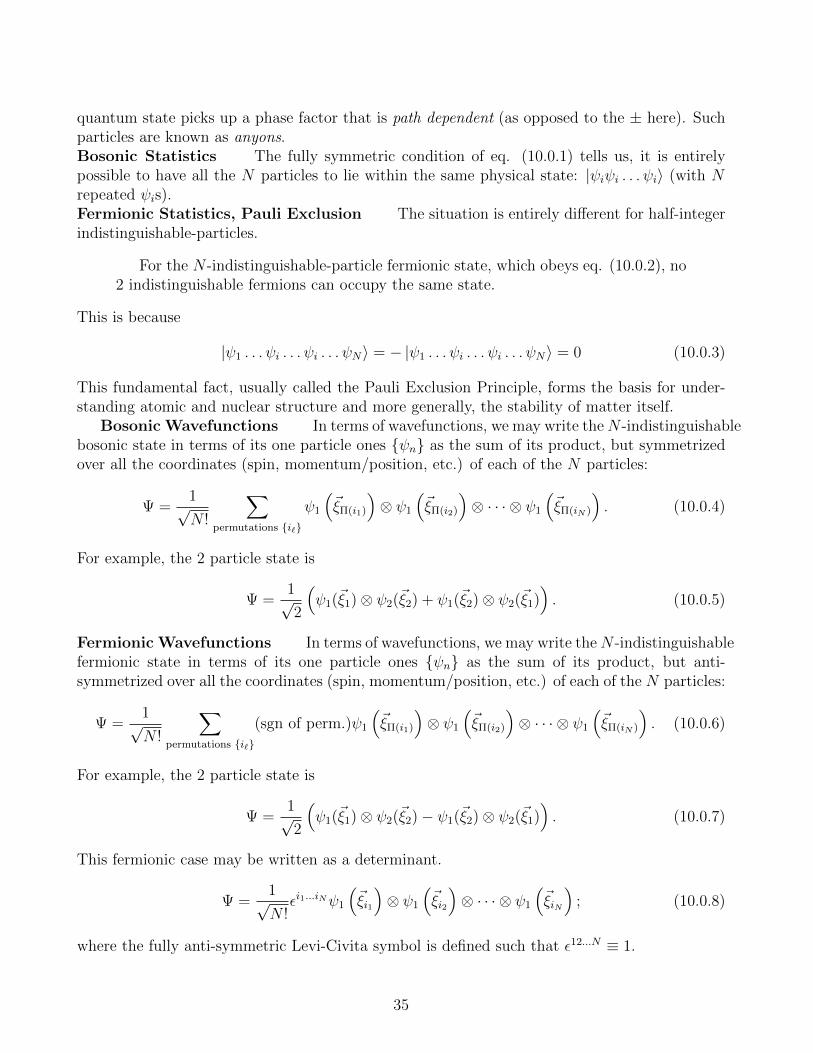
quantum state picks up a phase factor that is path dependent (as opposed to the ± here). Suchparticles are known as anyons.Bosonic Statistics The fully symmetric condition of eq. (10.0.1) tells us, it is entirelypossible to have all the N particles to lie within the same physical state: |ψiψi . . . ψi〉 (with Nrepeated ψis).Fermionic Statistics, Pauli Exclusion The situation is entirely different for half-integerindistinguishable-particles.
For the N -indistinguishable-particle fermionic state, which obeys eq. (10.0.2), no2 indistinguishable fermions can occupy the same state.
This is because
|ψ1 . . . ψi . . . ψi . . . ψN〉 = − |ψ1 . . . ψi . . . ψi . . . ψN〉 = 0 (10.0.3)
This fundamental fact, usually called the Pauli Exclusion Principle, forms the basis for under-standing atomic and nuclear structure and more generally, the stability of matter itself.
Bosonic Wavefunctions In terms of wavefunctions, we may write theN -indistinguishablebosonic state in terms of its one particle ones ψn as the sum of its product, but symmetrizedover all the coordinates (spin, momentum/position, etc.) of each of the N particles:
Ψ =1√N !
∑permutations i`
ψ1
(~ξΠ(i1)
)⊗ ψ1
(~ξΠ(i2)
)⊗ · · · ⊗ ψ1
(~ξΠ(iN )
). (10.0.4)
For example, the 2 particle state is
Ψ =1√2
(ψ1(~ξ1)⊗ ψ2(~ξ2) + ψ1(~ξ2)⊗ ψ2(~ξ1)
). (10.0.5)
Fermionic Wavefunctions In terms of wavefunctions, we may write theN -indistinguishablefermionic state in terms of its one particle ones ψn as the sum of its product, but anti-symmetrized over all the coordinates (spin, momentum/position, etc.) of each of the N particles:
Ψ =1√N !
∑permutations i`
(sgn of perm.)ψ1
(~ξΠ(i1)
)⊗ ψ1
(~ξΠ(i2)
)⊗ · · · ⊗ ψ1
(~ξΠ(iN )
). (10.0.6)
For example, the 2 particle state is
Ψ =1√2
(ψ1(~ξ1)⊗ ψ2(~ξ2)− ψ1(~ξ2)⊗ ψ2(~ξ1)
). (10.0.7)
This fermionic case may be written as a determinant.
Ψ =1√N !εi1...iNψ1
(~ξi1
)⊗ ψ1
(~ξi2
)⊗ · · · ⊗ ψ1
(~ξiN
); (10.0.8)
where the fully anti-symmetric Levi-Civita symbol is defined such that ε12...N ≡ 1.
35

10.1 Spin Precession and Rotating Fermions8Consider a spin-1/2 fermion with mass m. Let us consider its interaction with a magnetic field.Its Hamiltonian is given by, in units where ~ = 1 = c,
H = −gem~S · ~B; (10.1.1)
where ~S is the spin operator. The g is a particle-dependent constant; for e.g., Sakurai saysg ≈ 1.91 for the neutron.
If |±〉 are the eigenstates of ~S · ~B, namely
~S · ~B |±〉 = ±B2|±〉 , (10.1.2)
we have the stationary states
|E±(t)〉 = exp(−iHt) |±〉 = exp(ige
m(~S · ~B)t
)|±〉 (10.1.3)
= exp
(±igem
B
2t
)|±〉 . (10.1.4)
The factor of 1/2 occurring within the eigenvalue of ~S · ~B is due to the fermionic spin-1/2character of the particle. This same 1/2 is also responsible for multiplying the wavefunction by− upon a 2π rotation. For instance, if we rotate the spin eigenstates:
|±〉 → D(R(2π)) |±〉 ≡ exp(−i(2π)z · ~S) |±〉 (10.1.5)
|±〉 → exp(∓iπ) |±〉 = − |±〉 . (10.1.6)
Suppose we allow a fermion to propagate along two different paths, before recombining them toobserve the resulting interference pattern. Along one path we turn on a magnetic field over afinite region; and along the other we do not. If the initial state is prepared as a spin eigenstate(parallel to the ~B field); then, upon recombination, we must have
|±〉 → exp
(±igem
B
2T
)eiδ1 |±〉+ eiδ2 |±〉 (10.1.7)
= eiδ2 exp
(±igem
B
4T +
i
2(δ1 − δ2)
)×(
exp
(±igem
B
4T +
i
2(δ1 − δ2)
)+ exp
(∓igem
B
4T − i
2(δ1 − δ2)
))|±〉
= 2eiδ2 exp
(±igem
B
4T
)cos
(ge
m
B
4T + (δ1 − δ2)
)|±〉 . (10.1.8)
The T here is the time duration the particle spent inside the magnetic field. The spin−1/2character of the particle can be tested by testing the whether the change in magnetic field ∆Bwould cause a 2π phase shift in the interference pattern consistent with this result.
∆ϕ = 2π ⇔ ge
m
∆B
4T = 2π. (10.1.9)
8This section is based on Sakurai.
36

10.2 Atomic Structure/Periodic Table & Nuclear Structure
Electrons, neutrons and protons are fermions, obeying the Pauli exclusion principle. This playsa key role in the structure of atoms and nuclei.
For generic atomic number Z ≥ 1, to a decent approximation, the electrons move in aspherically symmetric central potential V (r). Near the nucleus, V (r) → −Ze2/r; whereasoutside the atom, V (r)→ −e2/r (i.e., screened by the other Z − 1 electrons). We may label thestates as follows
• Principal energy label n = 1, 2, 3, · · · ≥ 1.
• Orbital angular momentum ` ≥ 0; and ` ≤ n− 1.
• There are 2(2`+ 1) states for a fixed (n, `) pair, where 2 comes from the ±1/2 spin statesof the electron; and 2` + 1 coming from the range of L3 values. (This neglects spin-orbitinteractions.)
Unlike the hydrogen atom different ` but same n may not yield the same energy. As Weinbergexplains, oftentimes larger ` yields larger energies (for the same n), because the electron wavefunction goes as r` and hence spends less time near the origin. In order of increasing energy,i.e., E1 < E2 < · · · < E6 < E7,
Shell/E Level (n, `), Increasing in energy slightly → No. of states∑
2(2`+ 1)E1 1s = (1, 0) 2E2 2s = (2, 0), 2p = (2, 1) 2(1)+2(3)=8E3 3s = (3, 0), 3p = (3, 1) 2(1)+2(3)=8E4 4s = (4, 0), 3d = (3, 2), 4p = (4, 1) 2(1)+2(5)+2(3)=18E5 5s = (5, 0), 4d = (4, 2), 5p = (5, 1) 2(1)+2(5)+2(3)=18E6 6s = (6, 0), 4f = (4, 3), 5d = (5, 2), 6p = (6, 1) 2(1)+2(7)+2(5)+2(3)=32E7 7s = (7, 0), 5f = (5, 3), 7p = (7, 1), . . . . . .
Noble gases The chemically inert elements are those with their ’shells’ filled. These arehelium (Z = 2), neon (Z = 2+8 = 10), argon (Z = 2+8+8 = 18), krypton (Z = 2+8+8+18 =36, xenon (Z = 2 + 8 + 8 + 18 + 18 = 54), and radon (Z = 2 + 8 + 8 + 18 + 18 + 32 = 86).Alkaline metals Alkaline metals are those with one extra electron relative to the noblegases. This extra electron may be readily lost/roam easily throughout the metallic solid; thusmaking alkaline metals chemically reactive. These are lithium (Z = 2 + 1 = 3), sodium (Z =2 + 8 + 1 = 11), and potassium (Z = 2 + 8 + 8 + 1 = 19).Alkai Earths Alkali earths have two electrons more than noble gases: beryllium (Z =2 + 2 = 4), magnesium (Z = 2 + 8 + 2 = 12), and calcium (Z = 18 + 2 = 20).Halogens Halogens are elements with one fewer electron than the noble gases: fluorine(Z = 2 + 8− 1 = 9), chlorine (Z = 2 + 8 + 8− 1 = 17), bromine (Z = 2 + 8 + 8 + 18− 1 = 35).Oxygen & Sulfur Oxygen (Z = 10−2 = 9) and sulfur (Z = 18−2 = 16) have 2 electronsfewer than noble gases.
Nuclear Structure Inside the nucleus, we don’t have a central/core point-like charge.Instead it’s a bunch of protons and neutrons. If we do continue to approximate the potential as
37

a central one, i.e., V (r), and if we assume the origin is a stable point – we may Taylor expandit about the origin as follows:
V (r) = V0 + (ω2/2)r2 + . . . , ω2 ≡ V ′′(0). (10.2.1)
In other words, the nucleus near the origin should behave like a simple harmonic oscillator.Recall, for a fixed orbital angular momentum `, the 3D SHO oscillator energies go as
En,` = ω
(2n+ `+
3
2
), n = 0, 1, 2, . . . . (10.2.2)
Every adjacent energy level alternates between odd and even parity; so the ground state is evenparity, the first excited state is odd, and so on. This means odd ` shows up only for odd 2n+ `and even ` only for even 2n+ `.
Energy (relative to zero-point) ` No. of states∑
2(2`+ 1)0 s = 0 2ω p = 1 2(3)=62ω s = 0, d = 2 2(1)+2(5)=123ω p = 1, f = 3 2(3)+2(7)=20
The shell structure for nuclei is
Z = 2, 8, 20, 28, 50, 82, 126 (10.2.3)
where Z can refer to either protons or neutrons. For example, as Weinberg points out, 4He is‘doubly magic’ because it has Zp = 2 protons and Zn = 2 neutrons. This is why it is particularlystable; and is in turn why during the early universe nuclei heavier than 4He were not producedvery much. Other doubly magic nuclei are 16O and 40Ca; they are produced in stars morecopiously than their neighbors.
Note that our crude simple harmonic oscillator model can only explain the first 3 shells.According to Weinberg, as we move to the higher energy levels, not only does the potentialneeds to be modified, the spin-orbit ~S · ~L coupling becomes increasingly important. Remember,the total angular momentum j = `± 1/2. For ` = 3, that gives us j = 6/2± 1/2 = 5/2, 7/2.
11 Simple Harmonic Oscillator
11.1 One Dimension
The SHO system in 1D is defined by the Hamiltonian
H =1
2p2 +
1
2ω2x2. (11.1.1)
38

Energy Lower Bound To diagonalize this Hamiltonian, we first seek to “complete thesquare” in the following sense. Consider, for real α,(
1√2
(p− iαx)
)†(1√2
(p− iαx)
)=
1
2(p+ iαx) (p− iαx) (11.1.2)
=1
2
(p2 + α2x2
)+iα
2(xp− px) (11.1.3)
=1
2
(p2 + α2x2
)− α
2. (11.1.4)
Comparing the last line with eq. (11.1.1), we see that, by choosing α = ω,
H = ω
(1√2ω
(p− iωx)
)†(1√2ω
(p− iωx)
)+ω
2(11.1.5)
= ω
(a†a+
1
2
); (11.1.6)
where we have defined
a ≡ 1√2ω
(p− iωx) . (11.1.7)
We may immediately deduce
a† =1√2ω
(p+ iωx) . (11.1.8)
We may readily invert this relation to find
X = − i√2ω
(a† − a
)and P =
√ω
2
(a† + a
). (11.1.9)
At this point, we may infer from eq. (11.1.6) that there is a lower bound on the energy levelsof the SHO. If |E0〉 is the (unit norm) lowest energy eigenstate, and if we denote |Ψ〉 ≡ a |E0〉,then
〈E0 |H|E0〉 = E0 〈E0|E0〉 = E0 = ω
⟨E0
∣∣∣∣a†a+1
2
∣∣∣∣E0
⟩(11.1.10)
= ω
((a |E0〉)† (a |E0〉) +
1
2〈E0|E0〉
)(11.1.11)
= ω
(〈Ψ0|Ψ0〉+
1
2
)≥ ω
2. (11.1.12)
Raising & Lowering (aka “Ladder”) Operators The next step is to recognize the rolesof a and a† in equations (11.1.7) and (11.1.8), respectively, “lowering” and “raising” operators.[
a, a†]
=1
2ω[p− iωx, p+ iωx] (11.1.13)
= − iω2ω
([x, p]− [p, x]) (11.1.14)[a, a†
]= +1. (11.1.15)
39

Whereas
[H, a] = ω[a†a, a
]= ω
(a† [a, a] +
[a†, a
]a)
(11.1.16)
= ω[a†, a
]a = −ωa. (11.1.17)
Now [A,B]† = −[A†, B†], hence
−[H, a†
]= −ωa† (11.1.18)[
H, a†]
= ωa†. (11.1.19)
Now, if |En〉 is some energy eigenstate, a† |En〉 is an energy eigenstate with energy En+ω becauseof eq. (11.1.19):
H(a† |En〉
)=(Ha† − a†H + a†H
)|En〉 (11.1.20)
=([H, a†] + Ena
†) |En〉 =(ωa† + Ena
†) |En〉 (11.1.21)
= (En + ω)(a† |En〉
). (11.1.22)
Since a† |En〉 ∝ |En + ω〉, we must have (a†)† |En〉 = a†(a† |En〉) ∝ a† |En + ω〉 ∝ |En + 2ω〉; i.e.,in words: because each application of a† on an energy eigenstate yields an energy eigenstate withenergy +ω larger than the previous, ` ≥ 1 applications must yield
(a†)` |En〉 ∝ |En + `ω〉 . (11.1.23)
Likewise, if |En〉 is some energy eigenstate, a |En〉 is an energy eigenstate with energy En − ωbecause of eq. (11.1.17):
H (a |En〉) = (Ha− aH + aH) |En〉 (11.1.24)
= ([H, a] + Ena) |En〉 = (−ωa+ Ena) |En〉 (11.1.25)
= (En − ω) (a |En〉) . (11.1.26)
Iterating this reasoning ` times therefore hands us
a` |En〉 ∝ |En − `ω〉 . (11.1.27)
Since there is a lower bound on energy, however, this process cannot continue indefinitely. Sup-pose |E0〉 is the lowest energy eigenstate, because a |E0〉 cannot return a lower energy eigenstate,the only consistent answer is zero:
a |E0〉 = 0. (11.1.28)
Energies Recalling eq. (11.1.6), this means the lowest energy eigenstate must obey
E0 |E0〉 = ω
(a†a+
1
2
)|E0〉 =
ω
2|E0〉 ; (11.1.29)
i.e.,
E0 =ω
2. (11.1.30)
40

Every application of the raising operator adds ω to the energy level, we must have
En≥1 = ω
(n+
1
2
). (11.1.31)
Note that this discussion tells us there cannot be a separate infinite set of energy levels with alowest energy E0 + ε, where ε < E1−E0, where E0 is the lowest of all energies (by assumption).For, the lowering operator acting on it would again be zero, since E0 + ε−ω < E0. But then itsenergy is uniquely determined by ω(a†a+ (1/2)) |E0 + ε〉 = (ω/2) |E0 + ε〉.
Ground State Moreover, eq. (11.1.28) tells us
〈x |p− iωx|E0〉 = 0, (11.1.32)
−i∂x 〈x|E0〉 = iωx 〈x|E0〉 , (11.1.33)
∂x ln 〈x|E0〉 = −ωx, (11.1.34)
ln 〈x|E0〉 = −ω2x2 + constant, (11.1.35)
〈x|E0〉 = C exp(−ω
2x2), (11.1.36)
for some constant C. This constant may be fixed by demanding the wavefunction to have unitnorm. Taking C to be real,
〈E0|E0〉 = C2
∫ +∞
−∞e−ωx
2
dx = 1, (11.1.37)
C4
(∫ +∞
−∞e−ωx
2
dx
)2
= 1, (11.1.38)
C4
(∫R2
e−ω(x2+y2)dxdy
)= 1, (11.1.39)
C4
(2π
∫ +∞
0
e−ωρ2
ρdρ
)= 1, (11.1.40)
C4
(2π
−2ω
∫ +∞
0
∂
∂ρe−ωρ
2
dρ
)= 1, (11.1.41)
C4(πω
)= 1 ⇒ C =
(ωπ
) 14. (11.1.42)
To sum, up to an overall multiplicative phase, the non-degenerate ground state wavefunction is
〈x|E0〉 =(ωπ
) 14
exp(−ω
2x2), E0 =
ω
2. (11.1.43)
Excited States We already know from equations (11.1.8) and (11.1.23) that
〈x|En〉 ∝ (−i∂x + iωx)` 〈x|E0〉 . (11.1.44)
To normalize this state,((a†)` |E0〉
)† ((a†)` |E0〉
)=(a†(a†)`−1 |E0〉
)† ((a†)` |E0〉
)(11.1.45)
=((a†)`−1 |E0〉
)† (a(a†)` |E0〉
). (11.1.46)
41

Let us now prove the following statement:[a, (a†)`
]= ` · (a†)`−1. (11.1.47)
The ` = 1 case is simply the commutation relation [a, a†] = 1 in eq. (11.1.14). Assuming the(k > 1)th case is true, namely
[a, (a†)k
]= k · (a†)k−1,[
a, (a†)k+1]
= a†[a, (a†)k
]+[a, a†
](a†)k (11.1.48)
= a† · k · (a†)k−1 + (a†)k = (k + 1) · (a†)k+1. (11.1.49)
Returning to eq. (11.1.46), and keeping in mind eq. (11.1.28), we may now compute
a(a†)` |E0〉 =(a(a†)` − (a†)`a+ (a†)`a
)|E0〉 (11.1.50)
=[a, (a†)`
]|E0〉 = ` · (a†)`−1 |E0〉 ; (11.1.51)
and hence deduce that((a†)` |E0〉
)† ((a†)` |E0〉
)= ` ·
((a†)`−1 |E0〉
)† ((a†)`−1 |E0〉
)(11.1.52)
= `(`− 1) ·((a†)`−2 |E0〉
)† ((a†)`−2 |E0〉
)= . . . (11.1.53)
= `! 〈E0|E0〉 = `!. (11.1.54)
To sum: all unit norm excited states may be written as, for ` = 1, 2, 3, . . . ,
|E`≥1〉 =(a†)`√`!|E0〉 , E` = ω
(`+
1
2
). (11.1.55)
In the position representation,
〈x|E`〉 =(ω/π)1/4
√`!
(−i∂x − ωx√
2ω
)`exp
(−ω
2x2). (11.1.56)
Problem 11.1. Parity Explain why 〈−x|E`〉 = (−)` 〈x|E`〉.
Problem 11.2. Differential Equation for Excited States Guided by the result in eq.(11.1.56), we may infer that the excited state eigenfunction must take the following factorizedform:
〈x|E`〉 = Q`(ξ) 〈x|E0〉 , (11.1.57)
where ξ ≡√ωx. Show that Q`(ξ) obeys
Q′′` (ξ)− 2ξQ′`(ξ) + 2`Q`(ξ) = 0. (11.1.58)
By demanding that the ξ → ∞ limit yields a polynomial; and by comparing its highest powerwith that obtained with eq. (11.1.56), show that
Q`(ξ) =(ωπ
) 14
(i√2
)`H`(ξ)√`!, (11.1.59)
where H`(ξ) is the Hermite polynomial. Hint: The highest power of the Hermite polynomial canbe extracted from its power series in eq. 18.5.13 of NIST’s DLMF.
42

11.2 Schrodinger vs Heisenberg
Schrodinger Picture So far, we have been working within the Schrodinger picture where,if |ψ(t)〉s describes a physical system, it obeys the time dependent Schrodinger equation
i∂t |ψ(t)〉 = H |ψ(t)〉 , (11.2.1)
whose solution can be written in terms of the evolution operator
|ψ(t > t0)〉s = U(t, t0) |ψ(t0)〉s , (11.2.2)
where
U(t, t0) = exp(−iH(t− t0)); (11.2.3)
Most observables, such as the position and momentum operators, on the other hand, are time-independent. This means their eigenvectors are also time-independent.
Heisenberg Picture On the other hand, in the Heisenberg picture, we switch to a“rotating basis” of sorts, such that the state |ψ〉 describing the physical system no longer dependson time; but the operators such as position or momentum now do.
We will need to choose a time t0 where the two pictures coincide. The underlying motivationbehind the switching from Schrodinger to Heisenberg pictures is an alternate description of theexpectation value of some operator O. Starting in the Schrodinger picture,
s 〈ψ(t) |Os|ψ(t)〉 s = s
⟨ψ(t0)
∣∣e+iHs(t−t)Ose−iHs(t−t0)
∣∣ψ(t0)⟩
s ≡ H 〈ψ |OH|ψ〉 H; (11.2.4)
where the Heisenberg picture operator is
OH(t) ≡ e+iHs(t−t)Ose−iHs(t−t). (11.2.5)
We may obtain a first order differential equation for such a Heisenberg picture operator. As-suming its Schrodinger picture counterpart does not depend on time,
∂tOH(t) = i [HH, OH(t)] . (11.2.6)
Note that, for time independent Hamiltonians, their form is picture independent since theycommute at all times:
HH = eiHs(t−t0)Hse−iHs(t−t0) = eiHs(t−t0)e−iHs(t−t0)Hs = Hs. (11.2.7)
Also note that, the computation of commutators can be carried out in either picture; for operatorsA and B and denoting U(t, t0) ≡ exp(−iHs(t− t0)),
[AH, BH] = U(t, t0)†AsU(t, t0)U(t, t0)†BsU(t, t0)− U(t, t0)†BsU(t, t0)U(t, t0)†AsU(t, t0) (11.2.8)
= U(t, t0)† [As, Bs]U(t, t0). (11.2.9)
Spectra Since the Heisenberg operators depend on time, the observables now depend on timetoo. For example, the position operator is
XH(t) = e+iHs(t−t0)Xse−iHs(t−t0) (11.2.10)
43
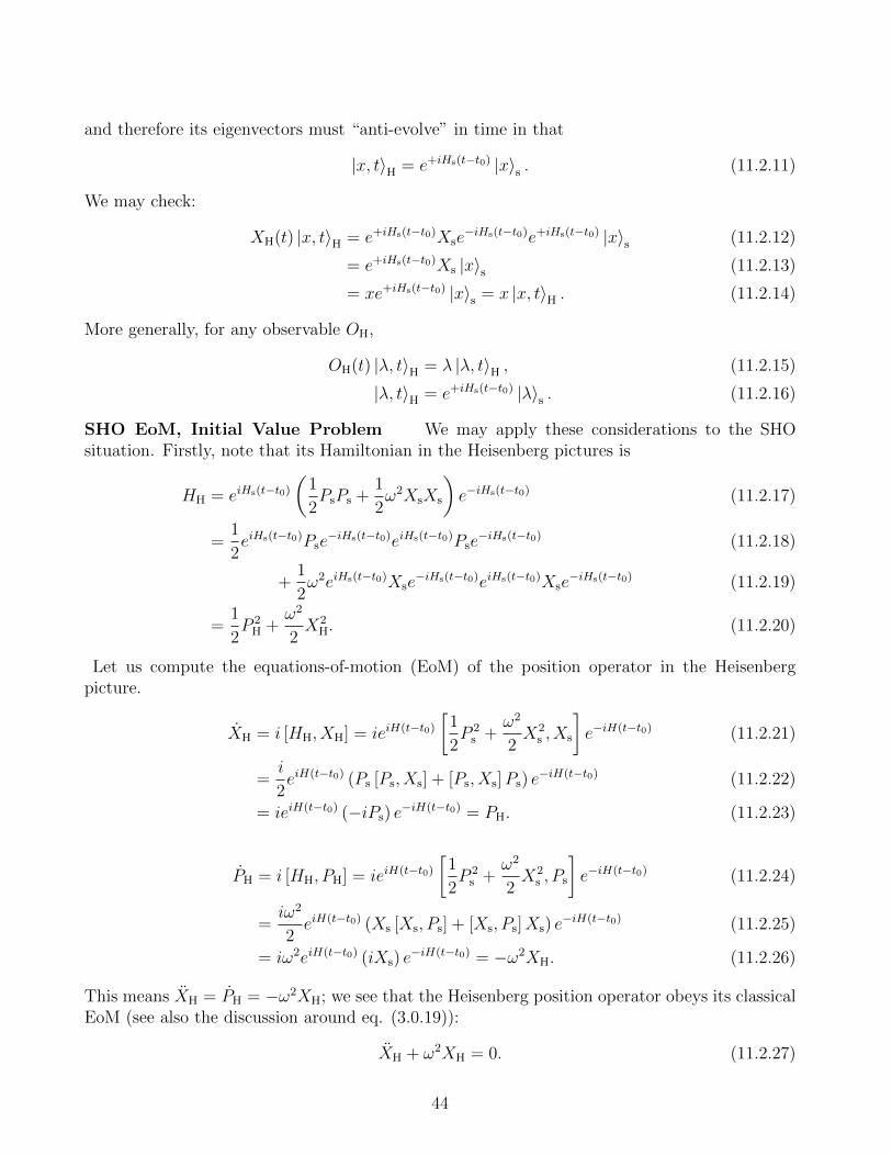
and therefore its eigenvectors must “anti-evolve” in time in that
|x, t〉H = e+iHs(t−t0) |x〉s . (11.2.11)
We may check:
XH(t) |x, t〉H = e+iHs(t−t0)Xse−iHs(t−t0)e+iHs(t−t0) |x〉s (11.2.12)
= e+iHs(t−t0)Xs |x〉s (11.2.13)
= xe+iHs(t−t0) |x〉s = x |x, t〉H . (11.2.14)
More generally, for any observable OH,
OH(t) |λ, t〉H = λ |λ, t〉H , (11.2.15)
|λ, t〉H = e+iHs(t−t0) |λ〉s . (11.2.16)
SHO EoM, Initial Value Problem We may apply these considerations to the SHOsituation. Firstly, note that its Hamiltonian in the Heisenberg pictures is
HH = eiHs(t−t0)
(1
2PsPs +
1
2ω2XsXs
)e−iHs(t−t0) (11.2.17)
=1
2eiHs(t−t0)Pse
−iHs(t−t0)eiHs(t−t0)Pse−iHs(t−t0) (11.2.18)
+1
2ω2eiHs(t−t0)Xse
−iHs(t−t0)eiHs(t−t0)Xse−iHs(t−t0) (11.2.19)
=1
2P 2
H +ω2
2X2
H. (11.2.20)
Let us compute the equations-of-motion (EoM) of the position operator in the Heisenbergpicture.
XH = i [HH, XH] = ieiH(t−t0)
[1
2P 2
s +ω2
2X2
s , Xs
]e−iH(t−t0) (11.2.21)
=i
2eiH(t−t0) (Ps [Ps, Xs] + [Ps, Xs]Ps) e
−iH(t−t0) (11.2.22)
= ieiH(t−t0) (−iPs) e−iH(t−t0) = PH. (11.2.23)
PH = i [HH, PH] = ieiH(t−t0)
[1
2P 2
s +ω2
2X2
s , Ps
]e−iH(t−t0) (11.2.24)
=iω2
2eiH(t−t0) (Xs [Xs, Ps] + [Xs, Ps]Xs) e
−iH(t−t0) (11.2.25)
= iω2eiH(t−t0) (iXs) e−iH(t−t0) = −ω2XH. (11.2.26)
This means XH = PH = −ω2XH; we see that the Heisenberg position operator obeys its classicalEoM (see also the discussion around eq. (3.0.19)):
XH + ω2XH = 0. (11.2.27)
44

Like its classical counterpart the solution may be written in terms of sine and cosine:
XH(t) = A cos (ω(t− t0)) +B sin (ω(t− t0)) ; (11.2.28)
except A and B are now operators. When t = t0 the sine vanishes and we must recover theSchrodinger picture position operator. This implies A = Xs. Whereas, since XH = PH =Aω sin(ω(t− t0)) +Bω cos(ω(t− t)), we must have when t = t0, B · ω = Ps. Altogether,
XH(t) = Xs cos (ω(t− t0)) +Ps
ωsin (ω(t− t0)) . (11.2.29)
This leads us to the following insight. Remember that the expectation value of some operatorO in the Heisenberg picture with respect to some physical state |ψ〉H = |ψ(t0)〉s is given by〈ψ0 |OH(t)|ψ0〉.
H 〈ψ|XH(t) |ψ〉 ,H = 〈ψ(t0)|Xs |ψ(t0)〉 cos (ω(t− t0))
+sin (ω(t− t0))
ω〈ψ(t0)|Ps |ψ(t0)〉 . (11.2.30)
At the level of expectation values, the Heisenberg picture position operator written in terms ofthe Schrodinger picture operators is simply the initial value formulation: 〈XH(t)〉 is the initial〈X〉 and 〈P 〉 (i.e., in the Schrodinger picture) evolved forward in time.
Problem 11.3. Show that eq. (11.2.29) may be expressed as
XH(t) =1√2ω
(α†eiω(t−t0) + αe−iω(t−t0)
), (11.2.31)
where α ≡ ia; with a being the lowering operator of equations (11.1.7), (11.1.8) and (11.1.9).In quantum field theory, each momentum mode of a given (linear) field operator obeys
something analogous to eq. (11.2.27); which in turn implies every momentum mode of thequantum field may be identified with eq. (11.2.31) – where, the raising/lowering operatorsbecome creation/destruction operators that create/destroy particles of the particular momentumat hand.
11.3 Higher Dimensions
The SHO in higher dimensions D > 1 is described by
H =1
2~P 2 +
ω2
2~X2. (11.3.1)
Spectrum Because this Hamiltonian is the sum of 1D ones, namely
H =1
2PiPi +
ω2
2X iX i, (11.3.2)
we may immediately take the tensor product of 1D SHO to diagonalize it:
|n1, . . . , nD〉 = |En1〉 ⊗ · · · ⊗ |EnD〉 , (11.3.3)
H |n1, . . . , nD〉 = En1,...,nD |n1, . . . , nD〉 = (En1 + . . . EnD) |n1, . . . , nD〉 (11.3.4)
= ω
(n1 + · · ·+ nD +
D
2
)|n1, . . . , nD〉 , (11.3.5)
45

where the n1, . . . , nD are a collection of non-negative integers. This is because, for a fixed i,(1
2PiPi +
ω2
2X iX i
)|n1, . . . , nD〉 (11.3.6)
=
(1
2PiPi +
ω2
2X iX i
)|En1〉 ⊗ · · · ⊗ |EnD〉 (11.3.7)
= |En1〉 ⊗ · · · ⊗(
1
2PiPi +
ω2
2X iX i
)|Eni〉 ⊗ · · · ⊗ |EnD〉 = Eni |n1, . . . , nD〉 . (11.3.8)
In the position representation, the corresponding unit norm energy wavefunction is
〈~x|n1, . . . , nD〉 =(ω/π)D/4√n1! . . . nD!
D∏i=1
(−i∂x − ωx√
2ω
)niexp
(−ω
2xixi
). (11.3.9)
Raising and Lowering Operators There are now D pairs of raising/lowering operators
ai =1√2ω
(Pi − iωX i
), (11.3.10)
a†i =1√2ω
(Pi + iωX i
). (11.3.11)
They obey [ai, a
†j
]= δij, [ai, aj] = 0 =
[a†i , a
†j
]; (11.3.12)
as well as
[H, ai] = −ωai and[H, a†i
]= +ωa†i . (11.3.13)
Parity Under parity ~x→ −~x, we have
〈−~x|n1, . . . , nD〉 = (−)n1+n2+···+nD 〈~x|n1, . . . , nD〉 . (11.3.14)
Three Dimensions We note that, because Ji and ~J2 commutes with the Hamiltonian, weexpect that the energy eigenstates 〈~x|n1, . . . , nD〉 can be built out of the former’s eigenstates.In 3D, this means we should be able to write
〈~x|n1, n2, n3〉 =∑`,m
χn1,n2,n3
`,m Rn1,n2,n3
`,m (r)Y m` (θ, φ). (11.3.15)
Examining eq. (11.3.9), we see that, for a fixed n1, n2, n3, the raising operators acting onthe Gaussian exp(−(ω/2)~x2) produces at most a degree n1 + n2 + n3 polynomial. Hence, themaximum ` in the above sum must be `max = n1 + n2 + n3. For each ` remember m runs overthe 2` + 1 values, from −` to +`. Whereas `min = 0; for example, (a†)2 exp(−(ω/2)x2) wouldproduce a constant term multiplying the gaussian. However, we have to remember eq. (11.3.14);
46

which in turn implies there must only even parity Y m` if N ≡ n1 + n2 + n3 were even and odd
parity Y m` if N were odd.
〈~x|n1, n2, n3〉 =N∑`=0` even
+∑m=−`
χn1,n2,n3
`,m Rn1,n2,n3
`,m (r)Y m` (θ, φ), Even N ≡ n1 + n2 + n3 (11.3.16)
=N∑`=1` odd
+∑m=−`
χn1,n2,n3
`,m Rn1,n2,n3
`,m (r)Y m` (θ, φ), Odd N ≡ n1 + n2 + n3. (11.3.17)
For even N this means there is 1 term for ` = 0; 2(2) + 1 for ` = 2; 2(4) + 1 for ` = 4; andaltogether
N/2∑k=0
(4k + 1) = 4N + 2
2
N
4+N + 2
2=
(N + 1)(N + 2)
2(11.3.18)
terms in the superposition of spherical harmonics to form eq. (11.3.9) of a fixed N .
Problem 11.4. Prove that, for odd N ≡ n1 + n2 + n3, there are also (N + 1)(N + 2)/2 termsin eq. (11.3.17).
Problem 11.5. N = 2 in 3D Write down all the wave functions 〈~x|N = 2, `,m〉, where
`(`+1) is the eigenvalue of ~J2 and −` ≤ m ≤ +` is that of J3, for a given energy ω(N+3/2).
Problem 11.6. Radial Wavefunction Let the energy eigenfunctions of the 3D SHO witheigenvalue E, namely 〈r, θ, φ|E〉, be
〈r, θ, φ|E〉 = R(√ωr)Y m
` (θ, φ) exp(−ω
2r2). (11.3.19)
Show that the radial wavefunction R obeys
R′′(ξ) +2
ξ(1− ξ2)R′(ξ)−
(3− 2E
ω+`(`+ 1)
ξ2
)R(ξ) = 0; (11.3.20)
where ξ ≡√ωr. Can you show the appropriate solutions are
R(ξ) = χn,` · ξ` 1F1
[−n, 3
2+ `, ξ2
]; (11.3.21)
where n is a non-negative integer and χn,` is a normalization constant. Explain why the energylevels are described by
E = ω
(2n+ `+
3
2
), n = 0, 1, 2, . . . . (11.3.22)
Using this energy eigenvalue result, and upon re-scaling R(ξ) = ξ`ρ(ξ2), show that ρ(ζ ≡ ξ2)satisfies the generalized Laguerre polynomial ODE
ζρ′′(ζ) +
(3
2+ `− ζ
)ρ′(ζ) + nρ(ζ) = 0. (11.3.23)
47

Hints: The ` = 0 case is already solved. Focus on ` > 0; and examine the r → 0 and r → ∞limits. You will find that one of the two linearly independent solutions, as r → 0, is notnormalizable. The other solution is not normalizable as r →∞ unless it becomes a polynomial.For this last step, you might need the fact that the Gamma function becomes singular at 0 andthe negative integers.
12 2-body Problem
Problem 12.1. In 2 body problems, where ~X1,2 refers to the positions and ~P1,2 to their corre-sponding momentum operators; show that the definitions
~R ≡ ~X1 − ~X2, (12.0.1)
~XCM ≡m1
~X1 +m2~X2
m1 +m2
(12.0.2)
and
~P ≡ ~P1 + ~P2 (12.0.3)
~ΠCM ≡ µ
(~P1
m1
−~P2
m2
), µ ≡ m1m2
m1 +m2
; (12.0.4)
lead to the position representations⟨~R, ~XCM
∣∣∣~P ∣∣∣ψ⟩ = −i∂ ~XCM
⟨~R, ~XCM
∣∣∣ψ⟩ , (12.0.5)⟨~R, ~XCM
∣∣∣~Π∣∣∣ψ⟩ = −i∂~R⟨~R, ~XCM
∣∣∣ψ⟩ . (12.0.6)
13 Rigid Body Dynamics in 3D Space
13.1 Classical
Setup By rigid body motion, I mean here a collection of point particles that are fixedin their positions relative to one another but may rotate as a whole around an arbitrary andpossibly time-dependent axis. Or a continuous material object that remains fixed in shapeand solid throughout its interior, but may rotate/change its orientation as a function of time.Quantitatively, if ~x(t) refers to a point within this rigid body, we say
xa(t) = Rab(t)xb, (13.1.1)
where Rab are components of a time-dependent rotation matrix; and xb are a set of time-independent coordinates that may be associated with that of the particle/location in questionbut relative to some frame co-rotating with the body itself.9
9More specifically, say at t = 0, we may view xa(t = 0) = Rab(t = 0)xb as the change-of-coordinates from theco-moving body frame coordinate system xa to the ‘ambient frame’ one xa.
48

Dynamics In reality, there must be some effective inter-particle potential that holdsthe body together; but within this rigid body assumption we may ignore it since all positions arefixed relative to the body-frame and whatever potential energy must become a constant in thislimit. Hence the dynamics must be entirely attributed to the kinetic energy, which we now seek.Focusing on the point particles case, we let the time-dependent coordinate of the nth particlebe denoted as ~x(n), such that
xa(n)(t) = Rab(t)xb(n). (13.1.2)
(Remember, the same rotation matrix Rab applies to all particles ~x(n) because they form arigid body.) Hence, if mn is the mass of the nth particle, its velocity is
xa(n)(t) = va(n) = Rab(t)xb(n); (13.1.3)
and total kinetic energy
K =1
2
∑n
mn~v2(n) (13.1.4)
=1
2
∑n
mnRap(t)Raq(t)xp(n)x
q(n) =
1
2NpqRapRaq; (13.1.5)
Nab ≡∑n
mnxa(n)x
b(n). (13.1.6)
We should be able to express this kinetic energy solely in terms of angular momentum variables,since the only motion under consideration is rotational. As a first step, we note that viewed asa matrix, the Rab obeys
RTR = I. (13.1.7)
Since this is true for all time, differentiating it once yields RTR+RTR = 0, which in turn implies
RTR = −RTR. (13.1.8)
On the other hand, since
RTR =(RTR
)T
, (13.1.9)
we see that RTR is an anti-symmetric matrix. In the 3D space we are in, this anti-symmetrymeans we may compute its dual:
Ωa =1
2εabc(RT)bfRfc; (13.1.10)
RfaRfb = εabcΩc. (13.1.11)
We may multiply both sides with Rib,
Ria = RibεabcΩc. (13.1.12)
49

Problem 13.1. Relation to vector calculus In vector calculus, we learn that the velocity~v(t) ≡ ~x(t) of some particle at ~x(t) due to rotation about some axis ω (where ω is a unit vector)with angular speed ω is given by
~x(t) = ~v(t) = ~ω(t)× ~x(t), ~ω ≡ ωω. (13.1.13)
Remember that xa(t) = Rab(t)xb and the cross product may be written in terms of the Levi-Civita tensor (in 3D flat space). Show that eq. (13.1.13) implies eq. (13.1.12) provided weidentify
~Ω = −~ω. (13.1.14)
Let us now express the kinetic energy in eq. (13.1.5) in terms of Ωa. Employing eq. (13.1.12),
K =1
2N ijRapεipqΩqRamεjmnΩn. (13.1.15)
Because of the orthogonality of the rotation matrices, RapRam = δpm.
K =1
2N ijεipqΩqεjpnΩn. (13.1.16)
Next we exploit the identity
εipqεjpn = δijδqn − δinδ
qj . (13.1.17)
to infer
K =1
2
(N iiδqn −Nnq
)ΩqΩn ≡ 1
2ΩqIqnΩn, (13.1.18)
Iab =∑n
mn
(xc(n)x
c(n)δ
ab − xa(n)xb(n)
). (13.1.19)
The Iab here is dubbed the moment-of-inertia tensor.
Problem 13.2. Compute the moment-of-intertia tensor (about the center-of-mass) for a tri-atomic system which we shall approximate as composed of 1 point mass m1 at
xa(1) = `(0, 0, 1); (13.1.20)
and 2 equal masses m2 at
xa(2±) =m1
m2
`
2(± tan(θ), 0,−1) . (13.1.21)
Verify that (0, 0, 0) is indeed the center-of-mass; and draw a figure to explain where these atomsare located.
50
Orbital angular momentum is
Ja(t) = εabc∑n
mnxb(n)(t)x
c(n)(t) (13.1.22)
= εabc∑n
mnRbp(t)xp(n)R
cq(t)xq(n) (13.1.23)
= εabc∑n
mnRbp(t)RcmεqmlΩlxp(n)x
q(n). (13.1.24)
From the co-factor expansion definition of the determinant, as well as the property of rotationmatrices that detR = 1,
εabcRapRbqRcl = εpql (13.1.25)
εcabRapRbq = Rclεpql. (13.1.26)
This in turn tells us
Ja(t) =∑n
mnRacεpmcεqmlΩlxp(n)x
q(n). (13.1.27)
Using eq. (13.1.17),
Ja(t) =∑n
mn(δpqδcl − δ
pl δcq)R
acΩlxp(n)xq(n) (13.1.28)
= Rac∑n
mn(xp(n)xp(n)δ
cl − xc(n)xl(n))Ω
l (13.1.29)
= RacIclΩl ≡ RacJ c. (13.1.30)
In matrix notation
J = RJ ⇔ RTJ = J . (13.1.31)
KE for invertible moment-of-inertia tensor We now notice that, if the moment-of-inertia tensor has an inverse, then
J a(I−1)abJ b = (IΩ)TI−1(IΩ) = ΩTII−1IΩ (13.1.32)
= ΩaIabΩb. (13.1.33)
Recalling the expression for the kinetic energy in eq. (13.1.18), we see that
K =1
2J a(I−1)abJ b. (13.1.34)
KE for non-invertible moment-of-inertia tensor Now, in a basis where Nab is diagonal,such that
Nab = diag(N1, N2, N3
); (13.1.35)
we have
Iab = diag(N2 +N3, N1 +N3, N1 +N2
). (13.1.36)
51

Problem 13.3. Starting from eq. (13.1.35), verify eq. (13.1.36).
We see that TrN =∑
nmn~x2(n) ≥ 0. This in turn says the sum of the eigenvalues of N are
always non-negative; in fact, all the eigenvalues are non-negative, i.e., N i ≥ 0. (Weinberg doesnot prove the latter assertion.) This in turn means, if Iab is non-invertible, since 2 out of the 3N is appear in every diagonal entry of Iab above, that means at least 2 out of 3 of them must bezero. This leaves only one non-zero component, which we shall simply denote at the 3rd:
Iab = diag(N3, N3, 0
), N1 = N2 = 0. (13.1.37)
In such a situation, we have
K =1
2Ω1I11Ω1 +
1
2Ω2I22Ω2 (13.1.38)
=1
2N3
(J 1)2
+(J 2)2
=1
2N3
~J 2 −
(J 3)2. (13.1.39)
13.2 Quantum
To quantize the rigid body dynamics, we shall treat the Rab as a 3 × 3 matrix of Hermitianoperators. We will assume they commute among themselves [Rab, Rpq] = 0; but not with thetime derivatives [Rab, Rpq] 6= 0. Moreover, the x(n)s – and, hence, the moment-of-inertia tensor– remain as numbers. This scheme will ensure the positions ~x(n)(t) commute among themselves;but not with their momentum.
We will in fact quantize the rigid body dynamics by appealing to the angular momentumalgebra: [
Ja, J b]
= iεabcJ c. (13.2.1)
Because position must transform as a 3-vector under rotation, we must also have[Ja, xb(n)
]= iεabcxc(n), (13.2.2)[
Ja, Rbd]xd(n) = iεabcRcdxd(n). (13.2.3)
But since these xd(n) are arbitrary, we deduce that the rotation operators are actually 3-vectors,for a fixed d: [
Ja, Rbd]
= iεabcRcd. (13.2.4)
In particular, when a = b, they commute with the angular momentum operators because theLevi-Civita is fully anti-symmetric. [
Ja, Rad]
= 0 (13.2.5)
This means when defining the J is as operators (cf. eq. (13.1.31)), namely
J a = J bRba, (13.2.6)
52

there is no operator-ordering ambiguity since the repeated index b means J bRba = RbaJ b. Thisallows us to write down the Hamiltonian of the rotator system immediately.
Hamiltonian for invertible moment-of-inertia tensor Because energy is entirelykinetic,
H =1
2J a(I−1)abJ b. (13.2.7)
Hamiltonian for non-invertible moment-of-inertia tensor In a basis where
Nab = diag(N1, N2, N3
); (13.2.8)
we have
Iab = diag(N2 +N3, N1 +N3, N1 +N2
). (13.2.9)
Setting N1 = N2 = 0,
Iab = diag(N3, N3, 0
). (13.2.10)
In turn,
H =1
2N3
(J 1)2
+(J 2)2
=1
2N3
~J 2 −
(J 3)2. (13.2.11)
Commutation Relations We now proceed to compute[Ja,J b
]=[Ja, J cRcb
]= [Ja, J c]Rcb + J c
[Ja, Rcb
](13.2.12)
= iεacdJdRcb + iεacdJ cRdb (13.2.13)
= iεacd(JdRcb − JdRcb). (13.2.14)
In other words [Ja,J b
]= 0. (13.2.15)
In particular, J3 and J 3 are compatible observables. Next,[J a,J b
]=[J a, J cRcb
]= [J a, J c]Rcb + J c
[J a, Rcb
](13.2.16)
=[J a, J cRcb
]= J c
[JeRea, Rcb
]= J c
[Je, Rcb
]Rea (13.2.17)
= iεecdJ cRdbRea = −iJ cRcdεabd. (13.2.18)
We have arrived at the commutation relations for the J s; they obey an angular-momentum-likeLie algebra: [
−J a,−J b]
= iεabc(−J c). (13.2.19)
Note, however, they are scalars under rotation because of eq. (13.2.15). On the other hand,because rotations are orthogonal transformations,
~J2 ≡ JaJa = J aJ a ≡ ~J 2. (13.2.20)
53

To sum: The ~J 2 = ~J2,J 3, J3 form a set of mutually compatible observables; with the Liealgebras of J is and −J is both obeying that of the 3D angular momenta. Their simultaneouseigenstates are
~J2 |J M K〉 = ~J 2 |J M K〉 = J(J + 1) |J M K〉 , (13.2.21)
J3 |J M K〉 = M |J M K〉 , and J 3 |J M K〉 = K |J M K〉 ; (13.2.22)
−J ≤M,K ≤ +J, M,K independent. (13.2.23)
Choosing a basis where Iab = diag(Ix, Iy, Iz) is diagonal,
H =(J x)2
2Ix+
(J y)2
2Iy+
(J z)2
2Iz(13.2.24)
= A ~J 2 +B(J z)2 + C((J x)2 − (J y)2
)(13.2.25)
A =1
4Ix+
1
4Iy, B =
1
2Iz− 1
4Ix− 1
4Iy, C =
1
4Ix− 1
4Iy(13.2.26)
Additionally,
(J x)2 − (J y)2 =1
2
(J +)2
+1
2
(J −)2
(13.2.27)
J ± ≡ J 1 ± iJ 2. (13.2.28)
Energy estimates From eq. (13.2.24) and the definition that I i ∼ (mass) × (inter-atomseparation distance)2, we may estimate the rotation energy levels of a molecule to go as
E ∼ (mNa2)−1, (13.2.29)
where mN is the typical mass of the nucleus (since that’s what dominates the mass of individualatoms) and a is the typical size of the molecule itself.
Problem 13.4. Explain why
~J 2 =∞∑J=1
∑−J≤M,K≤J
J(J + 1) |J M K〉 〈J M K| , (13.2.30)
(J 3)2 =∞∑J=1
∑−J≤M,K≤J
K2 |J M K〉 〈J M K| , (13.2.31)
(J ±)2 =∞∑J=1
∑−J≤M,K≤J
√J(J + 1)− (K ± 1)(K ± 2)
√J(J + 1)−K(K ± 1)
× |J M K ± 2〉 〈J M K| . (13.2.32)
Then use these results to diagonalize the Hamiltonian in eq. (13.2.24) for J = 1.
Problem 13.5. Toy model for triatomic molecule Find the rotational energy levels ofthe tri-atomic molecular system in Problem (13.2) for a state where ~J2 |J = 1〉 = ~J 2 |J = 1〉 =2 |J = 1〉.
Wavefunctions See Weinberg for now.
54

14 Entanglement & Bell’s Inequalities: Spin-Half Sys-
tems; EPR Paradox
One of the key features of quantum mechanics that distinguishes it from its classical counterpart,is the probabilistic character of its predictions. As we will now explore, the probabilistic characterof quantum mechanics is not mere randomness nor simply correlation – but entanglement. Weshall do so, following Sakurai and Napolitano [2], within the context of spin-half systems, whichinvolves the angular momentum generators
Si =σi
2. (14.0.1)
In the representation where σ3 is diagonal, the Pauli operators have the matrix representation
σ1 ≡[
0 11 0
], σ2 ≡
[0 −ii 0
], σ3 ≡
[1 00 −1
]. (14.0.2)
Suppose we begin with a spin-0 system, which then decays into two distinguishable spin-1/2particles. This means we may write our state as
∣∣0 0; 12
12
⟩and decompose it into the eigenstates
of the spin operators n · ~S ′ and n · ~S ′′ associated with the two decay products along the unitradial direction n.
n(θ, φ) ≡ (sin(θ) cos(φ), sin(θ) sin(φ), cos(θ)) (14.0.3)
From the rules of addition of angular momentum, we may express the decay through the equation∣∣∣∣0 0;1
2
1
2
⟩=
1√2
(|n+〉 ⊗ |n−〉 − |n−〉 ⊗ |n+〉) , (14.0.4)
where the first and second slots refers respectively to the first and second decay product. Wewill further suppose particle 1 and 2 flies off in opposite directions, so that we may measuretheir spins along some chosen directions, once they have become well separated in space. Thepossible outcomes of such a thought experiment would illustrate what quantum entanglementis, and why it is a distinct concept from mere correlations.
Problem 14.1. If |z, 1〉 ≡ |z+〉 and |z, 2〉 ≡ |z−〉 denotes the spin ‘up’ and ‘down’ states along
the z = (0, 0, 1) direction, verify that the eigenstates of n · ~S ≡ niSi are
ξ+A (n) ≡ 〈z,A| n+〉 =
(e−iφ cos (θ/2) , sin (θ/2)
)T(14.0.5)
and
ξ−A (n) ≡ 〈z,A| n−〉 =(−e−iφ sin (θ/2) , cos (θ/2)
)T; (14.0.6)
and that they obey the eigen-equation(n · ~S
)ξ± = ±1
2ξ±. (14.0.7)
55

According to equations (14.0.5) and (14.0.6),∑A=±
|z,A〉[e−iφ cos (θ/2) −e−iφ sin (θ/2)
sin (θ/2) cos (θ/2)
]A
B
≡∑A=±
|z,A〉UAB = |n,B〉 . (14.0.8)
Verify that the inverse relationship is
|z,+〉 = eiφ cos (θ/2) |n,+〉 − eiφ sin (θ/2) |n,−〉 , (14.0.9)
|z,−〉 = sin (θ/2) |n,+〉+ cos (θ/2) |n,−〉 . (14.0.10)
We will employ these results in the discussion on entanglement below.
Measurements Suppose the ~S · z of the first particle is measured, and it is found tobe +1/2. Then we know that the state of the system must be |z,+〉. If, now, the 2nd particle’s
S · n is measured. According to eq. (14.0.10),
|z,+〉 ⊗ |z,−〉 = sin (θ/2) |z,+〉 ⊗ |n,+〉+ cos (θ/2) |z,+〉 ⊗ |n,−〉 . (14.0.11)
That means the probability of obtaining +1/2 for the 2nd particle’s ~S · n is sin2(θ/2) and theprobability of −1/2 is cos2(θ/2).
On the other hand, if the first particle’s ~S · z were measured, and it were instead found tobe −1/2. Then according to eq. (14.0.9), the state becomes
|z,−〉 ⊗ |z,+〉 = eiφ cos (θ/2) |z,−〉 ⊗ |n,+〉 − eiφ sin (θ/2) |z,−〉 ⊗ |n,−〉 . (14.0.12)
If the ~S · ~n of the 2nd particle is then measured, the probability of obtaining +1/2 is cos2(θ/2)and −1/2 is sin2(θ/2).
Problem 14.2. Suppose we now have
n ≡ (sin θ cosφ, sin θ sinφ, cos θ) , (14.0.13)
n′ ≡ (sin θ′ cosφ′, sin θ′ sinφ′, cos θ′) . (14.0.14)
Use equations (14.0.9) and (14.0.10) to verify, the singlet state in eq. (14.0.4) can be expressedas∣∣∣∣0 0;
1
2
1
2
⟩=
1√2|n+〉 ⊗ |n′+〉 eiφ′
(ei(φ−φ
′) cos (θ/2) sin (θ′/2)− cos (θ′/2) sin (θ/2))
+1√2|n+〉 ⊗ |n′−〉 eiφ′
(ei(φ−φ
′) cos (θ/2) cos (θ′/2) + sin (θ′/2) sin (θ/2))
− 1√2|n−〉 ⊗ |n′+〉 eiφ
(ei(φ
′−φ) cos (θ/2) cos (θ′/2) + sin (θ′/2) sin (θ/2))
+1√2|n−〉 ⊗ |n′−〉 eiφ
(ei(φ
′−φ) cos (θ/2) sin (θ′/2)− cos (θ′/2) sin (θ/2)). (14.0.15)
Write down the probabilities P (n+, n′+), P (n+, n′−), P (n−, n′+), and P (n−, n′−). Since thecoordinate system is arbitrary, and since there are only two vectors in this problem, you mayassume they both lie on the (1, 3) plane; use this observation to show that all these probabilitiesdepend only on the angle θ between n and n′; namely, θ = arccos(n · n′).
56

Bell’s Inequality How does particle 2 ‘know’ what was being measured at particle 1?Once particle 1’s z · ~S is measured to be +1/2, for instance, then the z · ~S of particle 2 must turnout to be −1/2 – even if the time difference in the measurements of particles 1 and 2 were shorterthan the light crossing time between them. More generally, equations (14.0.11) and (14.0.12)indicate the probability of measuring ‘up’ or ’down’ for particle 2’s spin component along somedirection n′ depends (instaneously) on how it is oriented relative to the spin direction measuredfor particle 1. This apparent instant ’action-at-a-distance’ makes many physicists – includingEinstein himself – very uncomfortable, because it does not sit well with relativity.
Is it possible for a ’local’ theory to reproduce the predictions of quantum mechanics? Supposesuch a theory is able to produce seemingly probabilistic outcomes of spin, consistent with thepredictions of quantum mechanics. We will remain agnostic about the underlying mechanismof how it produces outcomes that appears random; but we will assume the outcome is alreadyfixed once the initial spin−0 particle decays. This is to ensure the theory is a ’local’ one:for, if the outcome were not already predetermined, it would mean the measurement processsomehow allows for a instantaneous influence-at-a-distance (for e.g., observing z+ for particle1 immediately causes z− for particle 2). As we shall see, this ‘Einstein locality principle’ leadsus to inequalities (named after its discoverer John Bell) involving the probabilities of obtainingvarious results that are in fact violated by quantum mechanics itself. In other words, there areobservable differences between such ‘local’ theories and quantum mechanics.
To see this, we need to consider three distinct detector orientations, which we shall denotea, b, and c. Such local theories, in order to be consistent with quantum mechanics, do notallow simultaneous measurements of spin along different directions. However, we shall assumethat particle 1 (and 2), when produced, will lead to definite outcomes for the spins measured
along a, b, and c. Let’s say out of a total N events, N1 produce particle 1 with the definiteoutcome a+, b+, c+ and particle 2 with definition outcome a−, b−, c−; N2 with a+, b+, c− anda−, b−, c+; etc – so that N =
∑iNi. (Note that the sum of particle 1 and 2’s spin components
must be zero; so we actually really only need to specify particle 1’s outcome.)
No. of events Decay Particle 1 Decay Particle 2
N1 a+, b+, c+ a−, b−, c−N2 a+, b+, c− a−, b−, c+N3 a+, b−, c+ a−, b+, c−N4 a+, b−, c− a−, b+, c+N5 a−, b+, c+ a+, b−, c−N6 a−, b+, c− a+, b−, c+N7 a−, b−, c+ a+, b+, c−N8 a−, b−, c− a+, b+, c+
We may see that the probability of obtaining spin up along a for particle 1; and spin up alongb for particle 2 is
P (a+ b+) =N3 +N4∑8
i=1Ni
≡ N3 +N4
N; (14.0.16)
57

while the probability for spin up along a for 1 and spin up along c for 2 is
P (a+ c+) =N2 +N4
N; (14.0.17)
and probability for spin up along c for 1 and b for 2 is
P (a+ c+) =N3 +N7
N. (14.0.18)
Since the Ni are non-negative, and hence N3 + N4 ≤ N2 + N3 + N4 + N7, this hands us anexample of Bell’s inequalities:
P (a+, b+) ≤ P (a+, c+) + P (c+, b+). (14.0.19)
See Sakurai [2] eq. (3.10.9), and the more detailed discussion that led up to it.
Problem 14.3. For simplicity, assume a, b and c all lie on the (1, 3) plane; and let θ1 denote the
angle between a and b and θ2 denote the angle between a and c. (Note: θ1 ∈ [0, π] and θ2 ∈ [0, π].)
Compute P (a+, b+), P (a+, c+), and P (c+, b+) in accordance to quantum mechanics, and figureout what region on the (θ1, θ2) Bell’s inequality is violated. Hint: See Problem (14.2).
Bonus: Can you find a Bell’s inequality different from that in eq. (14.0.19)? That is, find
probabilities for different set of observables (e.g., (a+, b−), (a−, b+), (c+, b−), etc.) that satisfytheir own inequalities. Does it get violated by quantum mechanics?
Correlation vs Quantum Entanglement Why did we have to examine the case wherethere are three distinct detector orientations? Suppose we had only examined the probabilityof obtaining P (a + b+), P (a + b−), P (a− b+), and P (a− b−). Let us again assume we had atheory that appears probabilistic but is local in the sense that, once the decay particles 1 and2 have been produced, their states are fixed. We may then draw a table of outcomes as we didbefore; where Ni∈1,2,3,4 is the number of events that yield the spin results of particles 1 and 2displayed in the corresponding 2nd and 3rd columns.
No. of events Decay Particle 1 Decay Particle 2 Probability Probability
N1 a+, b+ a−, b− P (a+, b−) P (b+, a−)
N2 a+, b− a−, b+ P (a+, b+) P (b−, a−)
N3 a−, b+ a+, b− P (a−, b−) P (b+, a+)
N4 a−, b− a+, b+ P (a−, b+) P (b−, a+)Table (14).
Because there are only 2 spin orientations considered here, we see that each possible outcomeis associated with a distinct probability. Contrast this with the 3 orientation case above, whereP (a + b+), P (a + c+), and P (c + b+) involved more than one Ni each. Therefore, in this 2detector orientations case, if the underlying theory is able to produce the same probabilitiesyou’ve computed in Problem (14.2), then it would be indistinguishable from quantum mechanics– as far as this simple system is concerned.
Problem 14.4. Identify the Ni∈1,2,3,4 in Table (14) with the probabilities computed in Problem(14.2).
Einstein–Podolsky–Rosen(-Bohm) Paradox & Causality What we have just wit-nessed is the entanglement between the spin properties of particle 1 and 2, produced upon thedecay of the original spin 0 object.
58

15 Path Integrals
Path integrals, sometimes also known as functional integrals, provide an alternate (but equiv-alent) formulation of quantum mechanics. This was pioneered by Richard Feynman as part ofhis PhD thesis.10 Path integration is usually not the most practical way to solve quantum me-chanical problems, but the perspective it offers is quite distinct from the Schrodinger-Heisenbergone – one no longer deals with operators and the recovery of classical mechanics follows almostimmediately from the stationary phase approximation. Also, in Quantum Field Theory (QFT),path integrals become an essential tool when dealing with the quantization of gauge theories.11
As we will demonstrate, the key object is the quantum mechanical amplitude for a particleto propagate from (t′, ~x′) to (t, ~x):
〈~x |U(t, t′)| ~x′〉 =
∫ ~x
~x′D~q∫D~p exp
[i
∫ t
t′
(~p(s) · ~q(s)−H (~q(s), ~p(s))
)ds
], (15.0.1)
where U is the unitary time-evolution operator which obeys Schrodinger’s equation
i∂tU(t, t′) = HU(t, t′) (15.0.2)
with the initial condition
U(t = t′) = I. (15.0.3)
The right hand side of eq. (15.0.1) is an integration over all possible trajectories ~q(s) – hence,path integration – that begins at (t′, ~x′) and ends at (t, ~x). The integration over ~p is unconstrained.The ~q is the position coordinate; ~p is its momentum; and H is the Hamiltonian of the dynamics.That the quantum mechanical amplitude is phrased as the sum over all possible paths, i.e.,Feynman’s formulation of quantum mechanics, is to be contrasted against the perspective of theusual Schrodinger’s wave function.
Problem 15.1. If K(t, ~x; t′, ~x′) is the quantum mechanical amplitude (aka path integral) from(t′, ~x′) to (t, ~x),
K(t, ~x; t′, ~x′) ≡ 〈~x |U(t, t′)| ~x′〉 ; (15.0.4)
explain why
(i∂t −H)G+(t, ~x; t′, ~x′) = iδ(t− t′)δ(D)(~x− ~x′), (15.0.5)
if
G+(t, ~x; t′, ~x′) ≡ Θ(t− t′)K(t, ~x; t′, ~x′). (15.0.6)
Here, Θ(z) = 1 for z > 0 and = 0 for z < 0.
10Norbert Wiener came up with the Euclidean version of the path integral before Feynman.11Some books dedicated to path integrals are: Feynman and Hibbs [3]; Schulman [4]; and Kleinert [5].
59

Lagrangian mechanics As is often the case, the H is quadratic in momentum; for e.g.,
H(~q, ~p) =~p2
2+ V (~q). (15.0.7)
12We may ‘complete-the-square’ within the exponent ~p · ~q −H,
~p · ~q − ~p2
2− V (~q) = −
(~p√2−√
2~q
2
)2
+ 2~q2
4− V (~q) (15.0.8)
= −
(~p√2−√
2~q
2
)2
+1
2~q2 − V (~q). (15.0.9)
The integration over ~p can be recognized as an overall multiplicative factor.
〈~x |U(t, t′)| ~x′〉 =
∫ ~x
~x′D~q∫D~p exp
[i
∫ t
t′
(~p(s) · ~q(s)− ~p2
2− V (~q)
)ds
](15.0.10)
=
∫ ~x
~x′D~q∫D
√
2
(~p√2−√
2~q
2
)
× exp
i ∫ t
t′
−( ~p√2−√
2~q
2
)2
+1
2~q2 − V (~q)
ds
(15.0.11)
= N∫ ~x
~x′D~q exp
[i
∫ t
t′
(1
2~q2(s)− V (~q(s))
)ds
]; (15.0.12)
where
N ≡∫D√
2~p′
exp
[−i∫ t
t′~p′2ds
]. (15.0.13)
In other words, in many cases of interest, the path integral reduces to one governed by theLagrangian of the dynamics of the particle.
〈~x |U(t, t′)| ~x′〉 = N∫ ~x
~x′D~q exp [iS] , (15.0.14)
S ≡∫ t
t′L(~q, ~q)
ds. (15.0.15)
In this sense, we have re-discovered Lagrangian mechanics from the Hamiltonian formulation ofquantum mechanics.
12We have deliberately set m = 1, because the same form of the Hamiltonian appears in relativistic QFT wherem does not appear like in the non-relativistic ~p2/(2m).
60

15.1 Example: Free Particle in Flat Euclidean Space
We will shortly begin to discuss in more detail what path integration really means. But let usfirst tackle the simplest such example: the free particle.
H(~q, ~p) =~p2
2m⇔ L(~q, ~q) =
m
2~q2 (15.1.1)
It is possible to evaluate the quantum mechanical amplitude directly. SinceH is time-independenthere, ⟨
~x
∣∣∣∣exp
[−i ~p
2
2m(t− t′)
]∣∣∣∣ ~x′⟩ =
∫dDk
(2π)D
⟨~x
∣∣∣∣exp
[−i ~p
2
2m(t− t′)
]∣∣∣∣~k⟩ 〈~k|~x′〉 (15.1.2)
=
∫dDk
(2π)Dexp
[−i~k2 t− t′
2m+ i~k · (~x− ~x′)
](15.1.3)
We can then complete the square
t− t′
2m~k2 − ~k · (~x− ~x′) =
√t− t′2m
~k − 1
2
√2m
t− t′(~x− ~x′)
2
− m
2(t− t′)(~x− ~x′)2 (15.1.4)
=t− t′
2m
~k − 1
2
2m
t− t′(~x− ~x′)
2
− m
2(t− t′)(~x− ~x′)2. (15.1.5)
And use analytic continuation of∫RD
dDz exp[−µ~z2] = (π/µ)D/2 (15.1.6)
to deduce, for t− t′ > 0 and m > 0,⟨~x
∣∣∣∣exp
[−i ~p
2
2m(t− t′)
]∣∣∣∣ ~x′⟩ = exp
[im
2(t− t′)(~x− ~x′)2
]e−i
π4D
(m
2π(t− t′)
)D/2; (15.1.7)
where the square root is the positive one.
Problem 15.2. Explain why, if ξ > 0,∫R
dz exp(±iξz2) = e±iπ4
√π
ξ, (15.1.8)
where the square root is the positive one. (Hint: this requires complex analysis and Jordan’slemma.) Why does this explain the phase factor e−iπD/4 in eq. (15.1.9)?
Now explain why, for arbitrary t− t′,⟨~x
∣∣∣∣exp
[−i ~p
2
2m(t− t′)
]∣∣∣∣ ~x′⟩ = exp
[im
2(t− t′)(~x− ~x′)2
]e−i
π4D·sgn[t−t′]
(m
2π|t− t′|
)D/2. (15.1.9)
The sgn[x] = +1 whenever x > 0; and sgn[x] = −1 whenever x < 0.
61

We may also start from the path integral itself.
N∫ ~x
~x′D exp
[i
∫ t
t′
m
2~q2ds
](15.1.10)
We will perform a change-of-variables
~q(s) = ~qc(s) + ~ξ(s) (15.1.11)
such that ~qc(s) obeys the ‘classical trajectory’
~qc(s) = 0, ~qc(t′) = ~x′, ~qc(t) = ~x. (15.1.12)
In fact, the solution is
~qc(s) = ~x′ +s− t′
t− t′(~x− ~x′). (15.1.13)
Since the ~q(s) in the path integral is defined to go from (t′, ~x′) to (t, ~x), that means the remainder~ξ has to be subject to the (Dirichlet) boundary conditions
~ξ(t′) = ~0 and ~ξ(t) = ~0. (15.1.14)
Let us focus on the action occurring within the path integral.
S =
∫ t
t′
m
2~q2ds =
∫ t
t′
m
2(~qc + ~ξ)2ds (15.1.15)
Using eq. (15.1.12),
S =
∫ t
t′
m
2~q2ds =
∫ t
t′
m
2
((~x− ~x′
t− t′
)2
+ 2~qc · ~ξ + ~ξ2
)ds (15.1.16)
=m
2
(~x− ~x′)2
t− t′+m
2
[2~qc · ~ξ
]tt′
+m
2
∫ t
t′
(−2~qc · ~ξ + ~ξ2
)ds. (15.1.17)
We have integrated-by-parts the second term within the integral because, according to the bound-ary conditions in eq. (15.1.14) obeyed by the ~ξ, the surface terms actually vanish. Moreover,
the classical ODE obeyed by ~qc (cf. eq. (15.1.12)) also eliminates the ~qc · ~ξ term.
S =m
2
(~x− ~x′)2
t− t′+m
2
∫ t
t′
~ξ2ds. (15.1.18)
To sum: the action occurring within the free particle path integral receives two contributions,one ‘classical’ portion (the first term on the RHS) due to a particle obeying constant accelerationmoving from (t′, ~x′) to (t, ~x); and another ‘quantum’ portion that propagates from (t′,~0) to (t,~0).Note that since ~qc is a fixed (i.e., classical) trajectory, it is a constant as far as the integrationover paths is concerned:
D~q = D~ξ. (15.1.19)
62

At this point, inserting eq. (15.1.18) into the right hand side of eq. (15.0.14), our path integralis ⟨
~x
∣∣∣∣exp
[−i ~p
2
2m(t− t′)
]∣∣∣∣ ~x′⟩ = N ′ exp
[im
2
(~x− ~x′)2
t− t′
](15.1.20)
N ′ ≡ N∫ ~0
~0
D~ξ exp
[im
2
∫ t
t′
~ξ2ds
]. (15.1.21)
We may in fact determine N ′ – without directly evaluating the⟨~0 |U |~0
⟩– up to an overall
multiplicative phase by recalling the transition amplitude may be regarded as the matrix elementof the unitary time evolution operator. In particular,
δ(D) (~x− ~y) =
∫RD
dD~x′⟨~x
∣∣∣∣exp
[−i ~p
2
2m(t− t′)
]∣∣∣∣ ~x′⟩⟨~y ∣∣∣∣exp
[−i ~p
2
2m(t− t′)
]∣∣∣∣ ~x′⟩ (15.1.22)
=
∫RD
dD~x′|N ′[t, t′]|2 exp
[im
2
(~x− ~x′)2 − (~y − ~x′)2
t− t′
](15.1.23)
= |N ′[t, t′]|2 exp
[im
2(t− t′)(~x2 − ~y2)
] ∫RD
dD~x′e−i(~x−~y)·~x′ mt−t′ . (15.1.24)
Recalling the integral representation of the Dirac delta-function, we arrive at
|N ′| =(
m
2π(t− t′)
)D/2. (15.1.25)
At this point, we gather from eq. (15.1.20),⟨~x
∣∣∣∣exp
[−i ~p
2
2m(t− t′)
]∣∣∣∣ ~x′⟩ = eiδ(t,t′)
(m
2π(t− t′)
)D/2exp
[im
2
(~x− ~x′)2
t− t′
](15.1.26)
Comparison between equations (15.1.9) and (15.1.26) allows us to see that the exponent exp(i m2(t−t′)(~x−
~x′)2) in the former comes entirely from the classical trajectory; and also lets us identify the phaseto be
exp(iδ(t, t′)) = e−iπ4D. (15.1.27)
Recall from eq. (15.0.14) that, up to an overall multiplicative factor,∫ ~0
~0
D~ξ exp
[im
2
∫ t
t′
~ξ2ds
]∝⟨~0 |U(t, t′)|~0
⟩(15.1.28)
=
⟨~0
∣∣∣∣exp
(−i ~p
2
2m(t− t′)
)∣∣∣∣~0′⟩ . (15.1.29)
This is of course what we did earlier, but now with ~x = ~x′ = ~0. In fact, we may re-write eq.(15.1.9) as⟨
~x
∣∣∣∣exp
[−i ~p
2
2m(t− t′)
]∣∣∣∣ ~x′⟩ = exp
[im
2(t− t′)(~x− ~x′)2
]⟨~0
∣∣∣∣exp
[−i ~p
2
2m(t− t′)
]∣∣∣∣~0⟩ ,⟨~0
∣∣∣∣exp
[−i ~p
2
2m(t− t′)
]∣∣∣∣~0⟩ = e−iπ4D
(m
2π(t− t′)
)D/2∝∫ ~0
~0
D~ξ exp
[im
2
∫ t
t′
~ξ2ds
]. (15.1.30)
63

15.2 Path Integrals From Time-Independent Hamiltonians
We now turn to a more systematic derivation of the path integral⟨~x∣∣∣e−iH(t−t′)
∣∣∣ ~x′⟩ =
∫ ~x
~x′D~q∫D~p exp
[i
∫ t
t′ds(~p · ~q −H [~p(s), ~q(s)]
)]. (15.2.1)
For technical simplicity we will assume H is time independent; we will also set the mass of theparticle to unity for technical convenience. The time independence of H means we may writethe quantum transition amplitude in eq. (15.2.1) as⟨
~x∣∣∣e−iH(t−t′)
∣∣∣ ~x′⟩ = limN→∞
⟨~x∣∣e−iH(δtN+δtN−1+···+δt2+δt1)
∣∣ ~x′⟩ , δt1 + · · ·+ δtN ≡ t− t′
= limN→∞
∫RD
dD~qN . . . dD~q2
⟨~x∣∣e−iHδtN ∣∣ ~qN⟩ ⟨~qN ∣∣e−iHδtN−1
∣∣ ~qN−1
⟩×⟨~qN−1
∣∣e−iHδtN−2∣∣ ~qN−2
⟩. . .⟨~q3
∣∣e−iHδt2∣∣ ~q2
⟩ ⟨~q2
∣∣e−iHδt1∣∣ ~x′⟩ . (15.2.2)
Now, we will assume that the position and momentum operators ( ~X and ~P ) within H has beenarranged such that ⟨
~q∣∣∣H ( ~X, ~P)∣∣∣~k⟩ = H
(~q,~k)〈~q|~k
⟩. (15.2.3)
This is not always true, but is certainly so for the common form of the Hamiltonian
H =1
2~P 2 + V ( ~X). (15.2.4)
With this assumption, and up to order δt,⟨~qi+1
∣∣e−iHδti∣∣ ~qi⟩=⟨~qi+1
∣∣∣1− iH ( ~X, ~P) δti +O(δt2)∣∣∣ ~qi⟩ (15.2.5)
=
∫dD~ki(2π)D
⟨~qi+1
∣∣∣1− iH ( ~X, ~P) δti +O(δt2)∣∣∣~ki⟩ ⟨~ki∣∣∣ ~qi⟩ (15.2.6)
=
∫dD~ki(2π)D
(1− iH
(~qi+1, ~ki
)δti +O(δt2)
)〈~qi+1|~ki
⟩ ⟨~ki
∣∣∣ ~qi⟩ (15.2.7)
=
∫dD~ki(2π)D
exp(i~ki (~qi+1 − ~qi)− iH
(~qi+1, ~ki
)δti
). (15.2.8)
This in turn implies eq. (15.2.2) turns into
⟨~x∣∣∣e−iH(t−t′)
∣∣∣ ~x′⟩ = limN→∞
∫RD
dD~qN . . . dD~q2
∫RD
dD~kN(2π)D
. . .dD~k1
(2π)D(15.2.9)
× ei~kN ·(~x−~qN )−iH(~x,~kN )δtN ei~kN−1·(~qN−~qN−1)−iH(~qN ,~kN−1)δtN−1
× ei~kN−2·(~qN−1−~qN−2)−iH(~qN−1,~kN−2)δtN−2 . . . ei~k1·(~q2−~x′)−iH(~q2,~k1)δt1
64

13This is what we mean by the path integration measures∫ ~x~x′D~q∫D~p in eq. (15.2.1). Notice
there is one more momentum than position integration, because there are no constraints on themomentum on the final/initial time slices.
Provided the operator ordering assumption in eq. (15.2.3) holds, the quantummechanical transition amplitude for a particle to propagate from ~x′ to ~x can be viewedas the limit of the continuous product over all times the exponential exp(i~p · ~q −H(~q, ~p)δt), integrated over all momentum and positions at each time slice – exceptthe end ~qs are held fixed at ~x′ and ~x.
Stationary Phase Approximation & Semi-Classical Limit For an ordinary integral,the Riemann–Lebesgue lemma tells us, if
f(x) ≡∫ b
a
exp(ixϕ(t))dt, (15.2.10)
where a and b are arbitrary real numbers and ϕ(t) is continuously differentiable and is notconstant over a finite region within the interval t ∈ [a, b]. Then
f(x→ +∞) = 0. (15.2.11)
We may understand this heuristically. As x→∞, the exponential oscillates wildly; and we mayin fact break the interval t ∈ [a, b] into small enough segments t ∈ [ti, ti+1] so that ϕ(t) is roughlya linear function of t in each of them and such that [ti, ti+1] corresponds exactly to one periodof exp(ixϕ(t)) ≈ exp(ix(a+ bt)). Then,∫ ti+1
ti
exp(ix(a+ bt))dt = 0 (15.2.12)
as x→ +∞. (This is also why there is a requirement that ϕ be non-constant everywhere withint ∈ [a, b]; otherwise the exponential will not oscillate there, and there is no period to integrateover to produce a zero result.)
General Formula In this limit as x → +∞, we may seek the leading behavior of thisintegral by searching for the point t0 such that
ϕ′(t0) = 0. (15.2.13)
For, in that region the ϕ is varies slower than first power in t, and∫ b
a
exp(ixϕ(t))dt =
∫ b
a
exp
(ix
ϕ(t0) +
1
2ϕ′′(t0)(t− t0)2 + . . .
)dt (15.2.14)
≈ eixϕ(t0)
∫R
exp(i(x/2)ϕ′′(t0)τ 2
)dτ. (15.2.15)
13There are subtleties related to this ‘time-slicing’ discretization approach to the path integral – see Kleinert [5]for more details. For example, the singular 1/r potential occurring within the Coulomb/Hydrogen-like problemyields more and more singular behavior at higher orders in δt.
65

Using the result in eq. (15.1.6) we see that this stationary phase approximation tells us
limx→+∞
∫ b
a
exp(ixϕ(t))dt ∼ exp[ixϕ(t0) + i
π
4sgn[ϕ′′(t0)]
]√ 2π
x|ϕ′′(t0)|, (15.2.16)
14One of the conceptual advantages of using the path integral in eq. (15.0.1) to discuss thequantum mechanical transition amplitude is the ease in which we may define the classical limit.A physical process is (semi-)classical when we may associate with it position ~q and momentum~p, such that the exponent in eq. (15.0.1) has magnitude much greater than unity, in units where~ ≡ 1: ∫ t
t′
(~p · ~q −H(~q, ~p)
)ds 1. (15.2.17)
When this criteria is filled, we may employ the stationary phase approximation to assert thatthe path integral is dominated by the stationary point, in the following sense. Let us consider
~x = ~Z + δ ~Z, (15.2.18)
~p = ~Π + δ~Π (15.2.19)
where δ ~Z and δ~Π are to be considered small perturbations relative to ~Z and ~Π respectively.Then,∫ t
t′
(~p · ~q −H(~q, ~p)
)ds =
∫ t
t′
(~Π · ~Z −H(~Z, ~Π)
)(15.2.20)
+ δ~Π ·(~Z − ∂H
∂~Π
)− δ ~Z ·
(~Π +
∂H
∂ ~Z
)+O
(δ ~Z2, δ~Π2, δ ~Zδ~Π
)ds+
[δ ~Z · ~Π
]s=ts=t′
.
We should view this step as the infinite dimensional version of the 1D one in eq. (15.2.14).Note that the last term is actually zero because of the boundary condition implied by the pathintegral in eq. (15.0.1), that ~Z(s = t) = ~x and ~Z(s = t′) = ~x′ – i.e., ~Z is fixed at the end points,
and thus δ ~Z vanishes there. At this point, we make the key observation: the stationary pointoccurs when the first order terms proportional to δ~Π and δ ~Z vanish. These yield the classicalHamilton’s equations:
~Z =∂H
∂~Πand ~Π = −∂H
∂ ~Z. (15.2.21)
Just as the dominant contribution to the integral in eq. (15.2.14) arises from the neighborhoodwhere ϕ′(t0) = 0, we see that the quantum mechanical amplitude for a particle to propagatefrom ~x′ to ~x is dominated by the classical solution – i.e., obeying Hamilton’s equations – subjectto the boundary conditions ~Z(t) = ~x and ~Z(t′) = ~x′.
14If there is no such t0 ∈ [a, b] such that ϕ′(t0) = 0, then f(x→ +∞) ∼ 1/x; i.e., the integral will decay morequickly than the case where a stationary point exists.
66

Quadratic-in-momentum & Lagrangian formulation The situation where H takesthe form in eq. (15.2.4) occurs frequently. If it holds, we may in fact ‘complete-the-square’ andobtain the Lagrangian formulation of the path integral⟨
~x∣∣∣e−iH(t−t′)
∣∣∣ ~x′⟩ = N∫ ~x
~x′D~q exp
[i
∫ t
t′dsL
(~q, ~q)]
, (15.2.22)
L(~q, ~q)
= ~p(~q) · ~q −H(~q, ~q). (15.2.23)
The first step is to recognize, if the Hamilton H does take the form in eq. (15.2.4) (this may
involve setting the mass to unity), then the exponential involving ~ki in eq. (15.2.9) can bewritten as
exp
(i
~ki ·
~qi+1 − ~qiδti
−~k2i
2− V (~qi+1)
δti
)(15.2.24)
= exp
(i
−1
2
(~ki −
~qi+1 − ~qiδti
)2
+(~qi+1 − ~qi)2
2δt2i− V (~qi+1)
δti
). (15.2.25)
Integrating over ~ki using eq. (15.1.6), and recognizing (~qi+1 − ~qi)/δti as the finite differenceapproximation of the velocity ~q(ti), we see that eq. (15.2.9) now reads
⟨~x∣∣∣e−iH(t−t′)
∣∣∣ ~x′⟩ = limN→∞
∫RD
dD~qN . . . dD~q2
N∏i=1
(e−i
πD4
(2πδti)D/2exp
(i
1
2~qi(ti)
2 − ~V (~qi)
δti
));
~qi(ti) ≡~qi+1 − ~qiδti
, ~q1 ≡ ~x′, and ~qN+1 ≡ ~x. (15.2.26)
(The square root is the positive one.) The shorthand for this expression is eq. (15.2.22).
Problem 15.3. Free Particle Path Integral Employ the result in eq. (15.2.26) toevaluate the path integral for the free particle, where V = 0. In other words, recover the resultin eq. (15.1.9). Hint: You may need to re-arrange the exponents; start integrating from ~q2, then~q3, etc.
Schrodinger’s Equation We may shift the final time t by an infinitesimal dt, andemploy the result in eq. (15.2.26) by treating the final time interval as δtN+1 ≡ dt.⟨~x∣∣∣e−iH(t+dt−t′)
∣∣∣ ~x′⟩= e−i
π4D
√1
2πdt
D ∫RD
dD~qN+1 exp
(i
(~x− ~qN+1)2
2dt− V (~x)dt
)⟨~qN+1
∣∣∣e−iH(t−t′)∣∣∣ ~x′⟩
= e−iπ4D
√1
2πdt
D ∫RD
dD~q′ exp
(i~q′2
2dt
)(1− iV (~x)dt+O(dt2)
) ⟨~q′ + ~x
∣∣∣e−iH(t−t′)∣∣∣ ~x′⟩
= e−iπ4D
√1
π
D ∫RD
dD~q′ exp(i~q′2) (
1− iV (~x)dt+O(dt2)) ⟨√
2dt~q′ + ~x∣∣∣e−iH(t−t′)
∣∣∣ ~x′⟩67

= e−iπ4D
√1
π
D ∫RD
dD~q′ exp(−(−i)~q′2
)(1− iV (~x)dt+O(dt))
×(
1 +√
2dt~q′ · ~∇~x +1
2(2dt)q′l1q′l2∂l1∂l2 +O(dt3/2)
)⟨~x∣∣∣e−iH(t−t′)
∣∣∣ ~x′⟩= e−i
π4D
√1
π
D ∫RD
dD~q′ exp(−(−i)~q′2
) (1 +√
2dt~q′ · ~∇~x + (dt)q′l1q′l2∂l1∂l2 − iV (~x)dt+O(dt3/2))
×⟨~x∣∣∣e−iH(t−t′)
∣∣∣ ~x′⟩ . (15.2.27)
We have ∫RD
dD~q′ exp(i~q′2)
=√πDe+iπD
4 . (15.2.28)
Additionally, because ei~q′2~q′ is odd in ~q′,∫
RDdD~q′ exp
(i~q′2)~q′ = 0; (15.2.29)
whereas ∫RD
dD~q′ exp(i~q′2)q′aq′b = Aδab; (15.2.30)
where A can be obtained by contracting both sides with respect to δab.∫RD
dD~q′ exp(i~q′2)~q′2 = A ·D (15.2.31)
−i∂λ∫RD
dD~q′ exp(iλ~q′2
)∣∣∣∣λ=1
= −i∂λ
√πi
λ
D∣∣∣∣∣λ=1
= D · A (15.2.32)
Therefore ∫RD
dD~q′ exp(i~q′2)q′aq′b = − i
D
(−D
2
)√πiDδab =
i
2
√πiDδab. (15.2.33)
Altogether, we now have⟨~x∣∣∣e−iH(t+dt−t′)
∣∣∣ ~x′⟩ =⟨~x∣∣∣e−iH(t−t′)
∣∣∣ ~x′⟩+ dt∂t
⟨~x∣∣∣e−iH(t−t′)
∣∣∣ ~x′⟩+O(dt2)
=
(1 + idt
1
2~∇2~x − V (~x)
+O(dt3/2)
)⟨~x∣∣∣e−iH(t−t′)
∣∣∣ ~x′⟩ . (15.2.34)
Equating the order dt terms on both sides, we obtain Schrodinger’s equation:
i∂t
⟨~x∣∣∣e−iH(t−t′)
∣∣∣ ~x′⟩ =
(−1
2~∇2~x + V (~x)
)⟨~x∣∣∣e−iH(t−t′)
∣∣∣ ~x′⟩ . (15.2.35)
In the other words, the path integral obeys the Schrodinger’s equation.
68

Heisenberg Picture Within the Heisenberg picture, recall that the position operator~XH(t) is time-dependent (unless it commutes with the Hamiltonian). Therefore, so are itseigenkets. According to eq. (3.0.22),
|~x, t〉H = U(t, t0)† |~x〉 . (15.2.36)
We see that the path integral in eq. (15.0.1) can be expressed as
H 〈~x, t| ~x′, t′〉H =
∫ ~x
~x′D~q∫D~p exp
[i
∫ t
t′
(~p · ~q −H(~q, ~p)
)ds
](15.2.37)
because
H 〈~x, t| ~x′, t′〉H =⟨~x∣∣U(t, t0)U(t′, t0)†
∣∣ ~x′⟩ (15.2.38)
= 〈~x |U(t, t0)U(t0, t′)| ~x′〉 = 〈~x |U(t, t′)| ~x′〉 . (15.2.39)
We have used the facts (cf. equations (2.0.11) and (2.0.12)) that
U(t1, t2)† = U(t2, t1) (15.2.40)
and
U(t1, t2)U(t2, t3) = U(t1, t3). (15.2.41)
Problem 15.4. What is∫dD~z
∫ ~x
~z
D~q exp
[i
∫ t
s
(1
2~q2 − V (~q)
)ds
] ∫ ~z
~x′D~q′ exp
[i
∫ s
t′
(1
2~q′2 − V (~q′)
)]? (15.2.42)
15.2.1 General Properties
Energy Eigenstates If we can perform the path integral exactly, this amounts to solving forthe energy eigenfunctions, as can be seen by inserting the completeness relation
∑n |En〉〈En| = I:
H 〈~x, t| ~x′, t′〉H = 〈~x |exp[−iH(t− t′)]| ~x′〉 (15.2.43)
=∑n
〈~x|En〉 〈En| ~x′〉 e−iEn(t−t′) (15.2.44)
H |En〉 = En |En〉 . (15.2.45)
Partition Function If we require that the particle start and end at the same point ~x =~x′ ≡ ~z, and then integrate over all space, we obtain the one-particle partition function:∫
dD~z H 〈~z, t| ~z, t′〉H =∑n
∫dD~z 〈En| ~z〉 〈~z|En〉 e−iEn(t−t′)
=∑n
e−iEn(t−t′). (15.2.46)
69

Green’s function and Determinants Assume for the moment that µ > 0, then consider∫ ∞0
dτe−µτ 〈~x |exp[−iHτ ]| ~x′〉 =∑n
〈~x|En〉 〈En| ~x′〉(e−iEnτ−µτ
−iEn − µ
)τ=∞
τ=0
(15.2.47)
=∑n
〈~x|En〉 〈En| ~x′〉µ+ iEn
(15.2.48)
We should be able to analytic continue the µ from real to “almost” purely imaginary µ →i(µ+ i0+), the 0+ ensuring convergence of the integral. Then we have
GF[~x, ~x′;µ] ≡ i
∫ ∞0
dτei(µ+i0+)τ 〈~x |exp[−iHτ ]| ~x′〉 (15.2.49)
=∑n
〈~x|En〉 〈En| ~x′〉En − µ− i0+
=
⟨~x
∣∣∣∣ 1
H − µ− i0+
∣∣∣∣ ~x′⟩ . (15.2.50)
Notice, when viewed as a complex function of µ, this object has simple poles at the energyeigenvalues µ = En − i0+. Furthermore, if H is the Hamiltonian in the position rep, we thenhave the Green’s function of the operator H − µ:
(H−µ)GF[~x, ~y;µ] =∑n
〈~x|En〉 〈En| ~x′〉 (15.2.51)
= δD[~x− ~x′]. (15.2.52)
Note that (En − ω)/(En − ω − i0+) = (En − ω)/(En − ω) + iπδ[En − ω](En − ω) = 1, becausezδ(z) = 0. In addition, if we trace over the positions and recall that the states |En〉 are of unitnorm, ∫
dDxGF[~x, ~x;µ] =∑n
1
En − µ− i0+≡ Tr
[1
H − µ
]. (15.2.53)
Operator Insertions If we ‘insert’ an operator OH(s) inside the transition amplitude
H 〈~x, t| ~x′, t′〉H, where t > s > t′, let us show that – provided O is diagonal in the positionrepresentation, namely
H
⟨~z, s
∣∣∣OH( ~X; s)∣∣∣ ~z′, s⟩
H= O (~z; s) δ(D) (~z − ~z′) , (15.2.54)
where the O on the right hand side takes the same form as that on the left except the positionoperator ~X has been replaced with ~z (or ~z′) – we have:
H 〈~x, t |OH(s)| ~x′, t′〉H =
∫ ~x
~x′D~q∫D~p O(s) exp
(i
∫ t
t′
~p · ~q −H[~p, ~q]
dτ
), (15.2.55)
t > s > t′. (15.2.56)
The analog of this object in Quantum Field Theory occurs frequently. Let us insert theHeisenberg-picture version of the completeness relation, i.e., eq. (3.0.24), on the left and rightof OH.
H 〈~x, t |OH(s)| ~x′, t′〉H
70
=
∫RD
dD~z
∫RD
dD~z′ H 〈~x, t| ~z, s〉H H 〈~z, s |OH(s)| ~z′, s〉H H 〈~z′, s| ~x′, t′〉H (15.2.57)
=
∫RD
dD~z
∫RD
dD~z′ H 〈~x, t| ~z, s〉H OH(~z; s)δ(D)(~z − ~z′) H 〈~z′, s| ~x′, t′〉H (15.2.58)
=
∫RD
dD~z H 〈~x, t| ~z, s〉H OH(~z; s) H 〈~z, s| ~x′, t′〉H . (15.2.59)
If we now exploit eq. (15.2.9),
H 〈~x, t |OH(s)| ~x′, t′〉H (15.2.60)
= limN→∞
∫RD
dD~qN . . . dD~q2
∫RD
dD~kN(2π)D
. . .dD~k1
(2π)D
× limN ′→∞
∫RD
dD~q′N ′ . . . dD~q′2
∫RD
dD~k′N ′
(2π)D. . .
dD~k′1(2π)D
×∫RD
dD~z O(~z; s)
× ei~kN ·(~x−~qN )−iH(~x,~kN )δtN ei~kN−1·(~qN−~qN−1)−iH(~qN ,~kN−1)δtN−1
× ei~kN−2·(~qN−1−~qN−2)−iH(~qN−1,~kN−2)δtN−2 . . . ei~k1·(~q2−~z)−iH(~q2,~k1)δt1
× ei~k′N′ ·(~z′−~q′N′ )−iH(~z′,~k′N′ )δt
′N′ei
~k′N′−1
·(~q′N′−~q
′N′−1
)−iH(~q′N′ ,
~k′N′−1
)δt′N′−1
× ei~k′N′−2
·(~q′N′−1
−~q′N′−2
)−iH(~q′N′−1
,~k′N′−2
)δt′N′−2 . . . ei
~k′1·(~q′2−~x′)−iH(~q′2,~k′1)δt′1
t− s ≡ δtN + · · ·+ δt1, s− t′ ≡ δt′N ′ + · · ·+ δt′1.
If O were simply the identity, we’d recover eq. (15.2.9). But with O present this merely meanswe’d have to, at the s-time-slice, also integrate over it. That is, eq. (15.2.60) is the continuumlimit of eq. (15.2.60).
Energy Eigenstates Expectation Values in Heisenberg Picture We may expressthe expectation value of some operator O with respect to an energy eigenket state in terms ofpath integrals. We will continue to assume eq. (15.2.54) holds; i.e., O is diagonal in the positionrepresentation. Specifically, keeping in mind eq. (15.2.55),
〈E |O|E〉 =
∫RD dD~x
∫RD dD~x′ 〈E| ~x〉 H 〈~x, t1 |OH(t)| ~x′, t2〉H 〈~x′|E〉
H 〈E, t1|E, t2〉H, (15.2.61)
H 〈E, t1|E, t2〉H =
∫RD
dD~x
∫RD
dD~x′ 〈E| ~x〉 H 〈~x, t1| ~x′, t2〉H 〈~x′|E〉 ; (15.2.62)
where t1,2 are arbitrary (as long as they are not equal to t) and the energy eigen-functions 〈~x|E〉are written in the Schrodinger picture. The situation in eq. (15.2.61) occurs frequently withinQFT, particularly when |E〉 refers to the vacuum state.
Using eq. (3.0.27), we begin with the numerator on the right hand side of eq. (15.2.61).∫RD
dD~x
∫RD
dD~x′ 〈E| ~x〉 H 〈~x, t1 |OH(t)| ~x′, t2〉H 〈~x′|E〉 (15.2.63)
=
∫RD
dD~x
∫RD
dD~x′ H 〈E, t1| ~x, t1〉 H H 〈~x, t1 |OH(t)| ~x′, t2〉H H 〈~x′, t2|E, t2〉 H (15.2.64)
71

Next we employ the Heisenberg-picture completeness relation in eq. (3.0.24).∫RD
dD~x
∫RD
dD~x′ 〈E| ~x〉 H 〈~x, t1 |OH(t)| ~x′, t2〉H 〈~x′|E〉 = H 〈E, t1 |OH(t)|E, t2〉 H (15.2.65)
Now, let us recall equations (3.0.9) and (3.0.22) to return to the Schrodinger picture.∫RD
dD~x
∫RD
dD~x′ 〈E| ~x〉 H 〈~x, t1 |OH(t)| ~x′, t2〉H 〈~x′|E〉 (15.2.66)
= 〈E| e−iE(t1−t0)eiE(t−t0)Oe−iE(t−t0)eiE(t2−t0) |E〉 (15.2.67)
= e−iE(t1−t2) 〈E|O |E〉 = 〈E| e−iE(t1−t0)eiE(t2−t0) |E〉 〈E|O |E〉 (15.2.68)
= H 〈E, t1|E, t2〉 H · 〈E|O |E〉 . (15.2.69)
Dividing both sides by H 〈E, t1|E, t2〉 H, we arrive at eq. (15.2.61). Moreover, when we setO = I on both sides, we have also recover the representation in eq. (15.2.62).
For time-independentH, the energy eigenstate expectation value of some operatorO in the Schrodinger picture can be expressed as a ratio of path integrals integratedagainst the energy-eigenfunctions at the initial and final times – with O inserted inthe numerator path integral.
Problem 15.5. Time-Ordered Products from Path Integrals Show that operatorinsertions within the path integral, namely∫ ~x
~x′D~q∫D~p exp
(i
∫ t
t′
~p · ~q −H[~q, ~p]
ds
)A(s)B(s′)C(s′′) . . . (15.2.70)
= H 〈~x, t |T AH(s)BH(s′)CH(s′′) . . . | ~x′, t′〉H ; (15.2.71)
where on the right hand side AH, BH, CH, . . . are arbitrary Heisenberg-picture operators diag-onal in the position representation; and A, B, C, . . . on the left-hand-side correspond to theircomplex-number counterparts; and t > (s, s′, s′′, . . . ) > t′. Whereas, T means the operatorswithin the curly brackets are arranged such that the ones with later times stand on the right.For instance, if s2 > s1, then
T AH(s1)BH(s2) = BH(s2)AH(s1); (15.2.72)
or, if s′′ > s > s′, then
T AH(s)BH(s′)CH(s′′) = CH(s′′)AH(s)BH(s′). (15.2.73)
Hint: Insert completeness relations using the position eigenkets in the Heisenberg-picture. Such“correlation functions” are central objects in QFT; for instance, through the Lehmann-Symanzik-Zimmermann reduction, one may obtain the quantum scattering amplitude of n particles.
72

15.2.2 Free Particle
We have already worked out the free particle path integral, so let us simply summarize thevarious representations here. From equations (15.1.3) and (15.1.9):⟨
~x
∣∣∣∣exp
[−i ~p
2
2m(t− t′)
]∣∣∣∣ ~x′⟩ =
∫ ~x
~x′D~q∫D~p exp
[i
∫ t
t′
(~p · ~q − ~p2
2
)ds
](15.2.74)
= N∫ ~x
~x′D~q exp
[i
∫ t
t′
m
2~q2ds
](15.2.75)
=
∫RD
dD~k
(2π)Dexp
[i~k · (~x− ~x′)− i
~k2
2m(t− t′)
](15.2.76)
= exp
[im
2(t− t′)(~x− ~x′)2
]e−i
πD4
sgn[t−t′](
m
2π|t− t′|
)D2
. (15.2.77)
15.2.3 Simple Harmonic Oscillator
In this section we are going to compute the path integral of the simple harmonic oscillator.Because the SHO Hamiltonian takes the form in eq. (15.2.4), with the potential being V (~q) =(ω2/2)~q2, we may thus start with the Lagrangian formulation in eq. (15.2.22):
KJ [t, t′; ~x, ~x′] ≡∫ ~x
~x′D~q exp [iS] ; (15.2.78)
where
S ≡∫ t
t′Lds; (15.2.79)
L ≡ 1
2
(~q[s]2 − ω2~q[s]2
). (15.2.80)
The strategy is as follows. Like the free particle case, we split the ~q into a classical ~qc andfluctuating piece ~ξ, so that
~q ≡ ~qc + ~ξ, (15.2.81)
D~q = D~ξ; (15.2.82)
with the boundary conditions
~qc[t′] = ~x′, ~qc[t] = ~x, ~ξ[t′] = ~ξ[t] = ~0. (15.2.83)
The Lagrangian now transforms into
L = L0 + ~qc · ~ξ − ω2~qc · ~ξ +1
2
(~ξ2 − ω2~ξ2
), (15.2.84)
L0 ≡1
2
(~q2c − ω2~q2
c
). (15.2.85)
73

The action now reads
S = S0 +[~ξ · ~qc
]tt′
+
∫ t
t′ds
− ~ξ ·
((d2
dt2+ ω2
)~qc
)+
1
2
(~ξ2 − ω2~ξ2
),
S0 ≡1
2
∫ t
t′
(~q2c − ω2~q2
c
)ds. (15.2.86)
We may demand that (d2
dt2+ ω2
)~qc = ~0. (15.2.87)
Problem 15.6. With the boundary conditions in eq. (15.2.83), verify that the solution to theclassical trajectory is
~qc[s] =~x sin [ω(s− t′)] + ~x′ sin [ω(t− s)]
sin [ω(t− t′)]; (15.2.88)
whenever the time elapsed is not a half-period, namely
ω(t− t′) 6= `π (for integer `). (15.2.89)
Next, show that the action now reads
S = Sc +
∫ t
t′ds
(1
2~ξ2 − ω2
2~ξ2
); (15.2.90)
where the classical contribution to the action is
Sc[~qc] =ω
2 sin [ω(t− t′)]((~x2 + ~x′2) cos [ω(t− t′)]− 2~x · ~x′
). (15.2.91)
Now, as long as t− t′ is not a half-period, eq. (15.2.89) is valid, our path integral now reads
K[t, t′; ~x, ~x′] = exp
[iω
2 sin [ω(t− t′)]((~x2 + ~x′2) cos [ω(t− t′)]− 2~x · ~x′
)]×∫ ~0
~0
D~ξ exp
[i
∫ t
t′ds
(1
2~ξ2 − ω2
2~ξ2
)]. (15.2.92)
Mode Sums & Functional Determinants We may now decompose ~ξ into a superpositionof the complete set of eigen-functions of (d/ds)2 + ω2, subject to the boundary condition in eq.
(15.2.83). Specifically, we may define the inner product of ~ξ1,2(s) to be⟨~ξ1
∣∣∣ ~ξ2
⟩≡∫ t
t′
~ξ1 · ~ξ2ds, (15.2.93)
~ξ1,2(s = t′) = ~0 = ~ξ1,2(s = t). (15.2.94)
74
In particular, the differential operator (d/ds)2 + ω2 is Hermitian∫ t
t′
(d2
ds2+ ω2
)~ξ1(s) · ~ξ2ds =
∫ t
t′
~ξ1(s) ·(
d2
ds2+ ω2
)~ξ2ds (15.2.95)
because the boundary terms vanishes by eq. (15.2.93).Moreover, the orthonormal eigenfunctions are
u`[s] =
√2
t− t′sin
[`π
t− t′(s− t′)
], (15.2.96)∫ t
t′um · unds = δmn, (15.2.97)(
d2
ds2+ ω2
)u` = −λ`u`, λ` ≡ ω2
`2
(π
ω(t− t′)
)2
− 1
. (15.2.98)
Since the eigen-functions of (d/ds)2 + ω2 must be complete,
~ξ =∞∑`=1
~Z`u`[s]. (15.2.99)
Note that u`[t] = u`[t′] = 0; and
(15.2.100)
Therefore,
1
2
∫ t
t′ds(~ξ2 − ω2~ξ2
)= −1
2
∞∑m,n=1
~Zm · ~Znδmn (−λn) =1
2
∞∑n=1
~Z2nλn; (15.2.101)
and
exp
[i
2
∫ t
t′
(~ξ2 − ω2~ξ2
)ds
]=
+∞∏`=1
exp
[i
2λ` ~Z
2`
]. (15.2.102)
We may now interpret, using eq. (15.2.98),∫ ~0
~0
D~ξ exp
[i
∫ t
t′ds
(1
2~ξ2 − ω2
2~ξ2
)]= N
+∞∏`=1
∫RD
dD ~Z` exp
[i
2λ` ~Z
2`
]
= N ′+∞∏`=1
eiDπ4
sgn[λ`]
∣∣∣∣∣ω2 −(
`π
t− t′
)2∣∣∣∣∣−D
2
(15.2.103)
Upon comparison with eq. (15.2.98), notice this ~0 → ~0 transition amplitude is proportional tothe −(D/2)th power of the product of the eigenvalues of the SHO operator (d/ds)2 +ω2 subject
to Dirichlet boundary conditions; this in turn is why the⟨~0 |U |~0
⟩is often dubbed a functional
75

determinant, since it is directly related to the determinant of the differential operator associatedwith the dynamics at hand.
det
(d2
ds2+ ω2
)≡∞∏`=1
(ω2 −
(`π
t− t′
)2)
(15.2.104)
∫ ~0
~0
D~ξ exp
[i
∫ t
t′ds
(1
2~ξ2 − ω2
2~ξ2
)]∝
det
(d2
ds2+ ω2
)−D2
. (15.2.105)
At this point, note that the pre-factors N and N ′ should not depend on ω, since it arises fromthe ambiguity of the integration measure D~ξ →
∏` dD ~Z`. We proceed as follows.
∫ ~0
~0
D~ξ exp
[i
∫ t
t′ds
(1
2~ξ2 − ω2
2~ξ2
)]= N ′
∞∏`′=1
(∣∣∣∣ `′πt− t′
∣∣∣∣−D e iDπ4 sgn[λ`′ ]
)+∞∏`=1
∣∣∣∣∣1−(ω(t− t′)
`π
)2∣∣∣∣∣−D
2
= N2[t− t′]∣∣∣∣ ω(t− t′)sin[ω(t− t′)]
∣∣∣∣D2 ,N2[t− t′] ≡ N ′
∞∏`′=1
(∣∣∣∣ `′πt− t′
∣∣∣∣−D e iDπ4 sgn[λ`′ ]
). (15.2.106)
We have utilized
sin z
z=∞∏`=1
(1− z2
(`π)2
). (15.2.107)
Let us observe that the sign of the eigenvalues in eq. (15.2.98),
λ` ≡ ω2
(π
ω(t− t′)
)2`2 −
(ω(t− t′)
π
)2, (15.2.108)
is controlled by the difference between the integer ` and ω(t − t′)/π (for t − t′ > 0). (Notethat, within classical dynamics, a full period t− t′ ≡ T of motion is determined by the equationωT = 2π; so t − t′ = π/ω is a half period.) When 0 < ω(t − t′)/π < 1, i.e., within the firsthalf-period, all the eigenvalues labeled by λ`|` = 1, 2, 3, . . . are positive and
N2[t− t′] ≡ N ′∞∏`′=1
(∣∣∣∣ `′πt− t′
∣∣∣∣−D e iDπ4). (15.2.109)
It is important to note that N2 depends on time but not on ω. This means we may determineits form by taking the ω → 0 limit,15 since it needs to recover the free particle case⟨
~x∣∣∣e−i(t−t′)~p2/2∣∣∣ ~x′⟩ =
∫RD
dD~k
(2π)Dei~k·(~x−~x′)e−i(t−t
′)~k2/2 (15.2.110)
15This is also why it is important to assume 0 < ω(t− t′) < π because, as we shall see, the other time intervals`π < ω(t− t′) < (`+ 1)π (for ` = 1, 2, 3, . . . ) are not continuously connected to the free particle ω = 0 case.
76

Denoting ~x− ~x′ ≡ ~R and t− t′ ≡ T , we first complete the square.
−T2
(~k − ~R
T
)2
− R2
T 2
= −T2
(~k2 − 2
T~k · ~R
)(15.2.111)
For T > 0, ⟨~x∣∣∣e−i(t−t′)~p2/2∣∣∣ ~x′⟩ = e
i2R2
T
∫RD
dD~k
(2π)De−i(t−t
′)~k2/2
= ei2R2
T
(e−i
π4
2π
√2π
|t− t′|
)D
. (15.2.112)
When ~x = ~x′ = ~0,
⟨~0∣∣∣e−i(t−t′)~p2/2∣∣∣~0⟩ =
(e−i
π4√
2π|t− t′|
)D
. (15.2.113)
and therefore, for 0 < ω(t− t′) < π, we have the result∫ ~0
~0
D~ξ exp
[i
∫ t
t′ds
(1
2~ξ2 − ω2
2~ξ2
)]= e−iD
π4
∣∣∣∣ 1
2π(t− t′)
∣∣∣∣D2 ∣∣∣∣ ω(t− t′)sin[ω(t− t′)]
∣∣∣∣D2 (15.2.114)
= e−iDπ4
∣∣∣∣ ω
2π sin[ω(t− t′)]
∣∣∣∣D2 . (15.2.115)
When the elapsed time t−t′ lies within the second half-period, 1 < ω(t−t′)/π < 2, then the firsteigenvalue λ1 in eq. (15.2.108) becomes negative whereas the rest of the λ`>1 remain positive.The overall amplitude N2 multiplying the SHO path integral in eq. (15.2.106) then reads
N2[t− t′] = N ′ ·
(∣∣∣∣ π
t− t′
∣∣∣∣−D e− iDπ4)·∞∏`′=2
(∣∣∣∣ `′πt− t′
∣∣∣∣−D e iDπ4)
(15.2.116)
= N ′∞∏`′=1
(∣∣∣∣ `′πt− t′
∣∣∣∣−D e iDπ4)e−i
π2D. (15.2.117)
The phase in the first factor has become e−i(πD)/4 = e+i(πD)/4e−i(πD)/2; and since N2 multipliesthe path integral, we see the quantum mechanical transition amplitude would therefore jumpby a phase e−i(πD/2) when the time elapsed t − t′ proceeds from the first to second half-period.In the third half-period, 2 < ω(t − t′)/π < 3, eq. (15.2.108) indicates both λ1 and λ2 are nownegative and
N2[t− t′] = N ′∞∏`′=1
(∣∣∣∣ `′πt− t′
∣∣∣∣−D e iDπ4)e−i2·
π2D. (15.2.118)
77

More generally, as t − t′ transitions from the `th half-period to the (` + 1)th one, the λ`+1
eigenvalue will flip sign from + to −, which in turn will cause a jump in the phase multiplyingthe path integral by e−i(πD/2). To sum, when
0 < ` <ω(t− t′)
π< `+ 1, (15.2.119)
the ~0 to ~0 path integral is∫ ~0
~0
D~ξ exp
[i
∫ t
t′ds
(1
2~ξ2 − ω2
2~ξ2
)]= e−i`
πD2 e−iD
π4
∣∣∣∣ ω
2π sin[ω(t− t′)]
∣∣∣∣D2 ; (15.2.120)
and eq. (15.2.92) becomes
K[t, t′; ~x, ~x′] = exp
[iω
2 sin [ω(t− t′)]((~x2 + ~x′2) cos [ω(t− t′)]− 2~x · ~x′
)]× e−i`
πD2 e−iD
π4
∣∣∣∣ ω
2π sin[ω(t− t′)]
∣∣∣∣D2 . (15.2.121)
Problem 15.7. SHO Path Integral & Classical Dynamics Recalling eq. (15.2.91), wemay write eq. (15.2.121) as∫ ~x
~x′D~q exp
[i
2
∫ t
t′
(~q2 − ω2~q2
)ds
]= e−i`
πD2 e−iD
π4
∣∣∣∣ ω
2π sin[ω(t− t′)]
∣∣∣∣D2 eiSc[~qc], (15.2.122)
` <ω(t− t′)
π< `+ 1. (15.2.123)
Show that, up to overall multiplicative phase factors, this result may be re-expressed as
H 〈~x, t| ~x′, t′〉H =
∫ ~x
~x′D~q exp
[i
2
∫ t
t′
(~q2 − ω2~q2
)ds
]=
(det
∂2Sc∂xa∂x′b
) 12
eiSc[~qc]. (15.2.124)
In other words – keeping in mind eq. (15.2.120) – the functional determinant⟨~0 |U |~0
⟩is also
directly related to the classical action differentiated with respect to the starting and endingpoints of motion. Eq. (15.2.124) is not a special feature of SHO dynamics, but a rather genericfeature of (the JWKB limit of) path integrals. The jump in the phase factors is also generic: itoccurs whenever one of the eigenvalues of the differential operator encoded in S flips sign.
Problem 15.8. One-particle Partition Function of SHO Recall that the energy levelsof the SHO are given by
En =
(n+
1
2
)ω (15.2.125)
in D = 1 dimension. First show that+∞∑`=1
e−i(t−t′)E` = (2i sin (ω(t− t′)/2))
−1. (15.2.126)
Then demonstrate that this is consistent with eq. (15.2.46), that the ‘trace’ of the path integralyields the one-particle partition function. Assume t− t′ is not a multiple of a half-period.
78

Half-Periods & Parity When ω(t− t′) = `π, we see the solution to path integral facesapparent infinities from all the occurrences of 1/ sin[ω(t− t′)] in eq. (15.2.121). This difficultlycan in turn be traced to the fact that the classical solution to the SHO – with boundary conditionsfixed – is no longer well defined. To see this, suppose ~x0 and ~x0 denote respectively the initialvelocity and position of the SHO at s = t′; then
~qc[s] =~x0
ωsin [ω(s− t′)] + ~x0 cos [ω(s− t′)] ,
(d2
ds2+ ω2
)~qc[s] = 0. (15.2.127)
At half-periods ω(s− t′) = `π, the dependence on the initial velocity drops out and
~qh[ω(s− t′) = `π] = ~x0(−)`. (15.2.128)
In other words, it is not possible to demand that, over the time duration t − t′ = `π/ω, a SHOparticle moves from ~x0 to some other ~x 6= (−)`~x0.
Let us see this from the path integral perspective. As we shall see, this result is intimatelyrelated to parity invariance of the SHO Hamiltonian. To begin, let us define in the Schrodingerpicture
P |~x〉 ≡ |−~x〉 . (15.2.129)
Note that, if ~X is the position operator, this is equivalent to
P−1 ~XP = − ~X. (15.2.130)
Also observe that
P 2 |~x〉 = P |−~x〉 = |~x〉 ⇒ P−1 = P. (15.2.131)
We may readily construct the symmetric and antisymmetric eigenstates of P as
|~x; +〉 ≡ |~x〉+ |−~x〉√2
and |~x;−〉 ≡ |~x〉 − |−~x〉√2
. (15.2.132)
How does the parity operator acts on the momentum eigenstates ∣∣∣~k⟩? We consider⟨
~k |P | ~x⟩
=⟨~k∣∣∣− ~x⟩ = χe−i
~k·(−~x) = χe−i(−~k)·~x =
⟨−~k∣∣∣ ~x⟩ . (15.2.133)
Since this is true for any |~x〉, we must have
P∣∣∣~k⟩ =
∣∣∣−~k⟩ ; (15.2.134)
and for momentum operator ~p
P~pP = −~p. (15.2.135)
79

Since the position and momentum operators transform in the same manner, and since the rais-ing/lowering operators are formed from their linear combinations, this implies the ~a and ~a† inequations (11.3.10) and (11.3.11) also transform as
P~aP = −~a, P~a†P = −~a†. (15.2.136)
We may use the fact that the ground state |E0〉 is even under parity16 to see that each higherstate would alternate between odd and even under parity. For instance, if (ai`)† is the raisingoperator in the `th spatial direction,
P (ai1)† . . . (ain)† |E0〉 = P (ai1)†P · P (ai2)†P . . . P (ain−1)†P · P (ain)†P 2 |E0〉= (−)n(ai1)† . . . (ain)†P |E0〉 = (−)n(ai1)† . . . (ain)† |E0〉 . (15.2.137)
For ω(t− t′) = `π, we may now analyze our path integral as follows
K[ω(t− t′) = `π; ~x, ~x′] = 〈~x| exp
[−i`π
ωHSHO
]|~x′〉 ,
=∞∑
n1,...,nD=0
〈~x|E~n〉 〈E~n| ~x′〉 exp
[−i`π
(n1 + · · ·+ nD +
D
2
)]
=1
iD·`
∞∑n1,...,nD=0
〈~x|E~n〉 〈E~n| ~x′〉 (−)(n1+···+nD)·`
=1
iD·`
∞∑n1,...,nD=0
〈~x|E~n〉⟨E~n∣∣P `∣∣ ~x′⟩
=1
iD·`
∞∑n1,...,nD=0
〈~x|E~n〉 〈E~n| (−)`~x′⟩. (15.2.138)
But the summation is now the completeness relation:
K[ω(t− t′) = `π; ~x, ~x′] =1
iD·`δ(D)
[~x− (−)`~x′
], (15.2.139)
where D is the number of space dimensions.Summary The transition amplitude for the SHO system
〈~x |exp [−i(t− t′)HSHO]| ~x′〉 =
∫ ~x
~x′D~q exp
[i
2
∫ t
t′
(~q2 − ω2~q2
)ds
](15.2.140)
is given by, for the first half-period,
〈~x |exp [−i(t− t′)HSHO]| ~x′〉 (15.2.141)
= e−iDπ4
∣∣∣∣ ω
2π sin[ω(t− t′)]
∣∣∣∣D2 exp
[iω
2 sin [ω(t− t′)]((~x2 + ~x′2) cos [ω(t− t′)]− 2~x · ~x′
)]≡ K0[t, t′; ~x, ~x′], 0 < t− t′ < π
ω; (15.2.142)
16Up to overall numerical/normalization constants, 〈~x|E0〉 ∝ exp[−ω~x2/2].
80

and for subsequent half-periods,
〈~x |exp [−i(t− t′)HSHO]| ~x′〉 =1
iDK0[t, t′; ~x, ~x′],
π
ω< t− t′ < 2π
ω, (15.2.143)
=1
i2DK0[t, t′; ~x, ~x′],
2π
ω< t− t′ < 3π
ω, (15.2.144)
=1
i3DK0[t, t′; ~x, ~x′],
3π
ω< t− t′ < 4π
ω, (15.2.145)
. . . . . . (15.2.146)
17When the time elapsed is exactly a multiple of a half-period, t − t′ = `π/ω and integer` = 1, 2, 3, . . . ,
〈~x |exp [−i(t− t′)HSHO]| ~x′〉 =1
iD·`δ(D)
[~x− (−)`~x′
]. (15.2.147)
16 Acknowledgments
A Classical Mechanics of a Point Particle: Review
In this section, I shall provide a review of the classical mechanics of point particles.Lagrangian Mechanics Let us start by assuming the variational principle, which is
encapsulated within the Lagrangian L. We shall suppose L only depends on the trajectory ~q(t)and its velocity ~q(t), but not on its higher time derivatives.
The extremum of the action leads to the Euler-Lagrange equations
∂L
∂qi=
d
dt
∂L
∂qi. (A.0.1)
Hamiltonian Dynamics The momentum conjugate to ~q is defined as
pi ≡∂L(~q, ~q)
∂qi. (A.0.2)
This eq. (A.0.2) will usually allow us to solve ~q in terms of ~q and ~p. In turn, the Hamiltonianis defined as
H(~q, ~p) = piqi(~q, ~p)− L (~q, ~p) . (A.0.3)
Note that, since we have switched variables from (~q, ~q) to (~q, ~p), we need to understand how thepartial derivatives in eq. (A.0.1) are altered. Viewed as a function of (~q, ~q),
δH(~q, ~q) = δpiqi + piδq
i −
(∂L(~q, ~q)
∂qi
)~q
δqi −
(∂L(~q, ~q)
∂qi
)~q
δqi
= δpiqi + piδq
i − d
dt
(∂L(~q, ~q)
∂qi
)~q
δqi − piδqi
= δpiqi − piδqi (A.0.4)
17These phase jumps are related to the Maslov-Morse indices; see [6] for a pedagogical discussion.
81

Whereas, when viewed as a function of (~q, ~p),
δH(~q, ~p) =
(∂H
∂qi
)~p
δqi +
(∂H
∂pi
)~q
δpi. (A.0.5)
Comparing the two expressions then hands us Hamilton’s equations:
qi =∂H(~q, ~p)
∂pi, (A.0.6)
pi = −∂H(~q, ~p)
∂qi. (A.0.7)
Poisson brackets & Hamiltonian flow The Poisson bracket between two functions (f, g)of (~q, ~p) is defined as
f, gPB ≡∂f(~q, ~p)
∂qi∂g(~q, ~p)
∂pi− ∂f(~q, ~p)
∂pi
∂g(~q, ~p)
∂qi. (A.0.8)
We now see that, using these Poisson brackets, that the Hamilton ‘generates’ time evolution:
f,HPB =∂f
∂qi∂H
∂pi− ∂f
∂pi∂H
∂qi
=∂f
∂qiqi +
∂f
∂pipi =
df (~q(t), ~p(t))
dt. (A.0.9)
Spatial translations & Momentum flow Using the Poisson brackets, we may also showthat momentum generates spatial displacements in that
f, p`PB =∂f
∂qi∂p`∂pi− ∂f
∂pi∂p`∂qi
=∂f
∂q`. (A.0.10)
Electromagnetism of Point Particles In Minkowski spacetime, the relativistic actionfor a point electric charge e is given by
S =
∫dt(−m√
1− ~v2 + e ~A · ~v − eφ). (A.0.11)
Here, m is its mass; ~v ≡ d~q/dt its spatial velocity; ~A is the vector potential; and φ ≡ A0 is theelectric potential (and also the zeroth component of the vector potential). In the non-relativisticlimit, we have
S =
∫dt(−m+ LEM +O(v4)
), (A.0.12)
where the Lagrangian is
LEM ≡m
2~v2 + e ~A · ~v − eφ. (A.0.13)
82

Problem A.1. Electromagnetic Hamiltonian Using the definition in eq. (A.0.2),namely
~p ≡ ∂LEM
∂~v, (A.0.14)
show that
~v =1
m
(~p− e ~A
). (A.0.15)
From this result, show that the HamiltonianHEM associated with the electromagnetic Lagrangianin eq. (A.0.13) is
HEM =1
2m
(~p− e ~A
)2
+ eφ. (A.0.16)
Eq. (A.0.16) is often the starting point of electromagnetism in the quantum mechanics.
We may check the consistency of the classical Hamiltonian in eq. (A.0.16) by computing itsHamilton’s equations. Applying eq. (A.0.6) recovers eq. (A.0.15); while employing eq. (A.0.7)yields
~p = −∂HEM
∂~q= − 1
m(pi − eAi) (−e)~∇~qAi − e~∇~qφ. (A.0.17)
Utilizing eq. (A.0.15) once again,
~p = evi~∇~qAi − e~∇~qφ (A.0.18)
d
dt
(m~v + e ~A(t, ~q)
)= evi~∇~qA
i − e~∇~qφ. (A.0.19)
Now, d ~A/dt = ∂t ~A+ va∂a ~A. Hence, we arrive at
mvi = e(vm∂iA
m − vm∂mAi − ∂tAi − ∂iφ). (A.0.20)
If we remember the relationship between the electric and magnetic fields with that of the vectorpotential, namely
Ei = −∂iφ− ∂tAi and Bi = εimn∂mAn, (A.0.21)
we recover the familiar Lorentz force law:
mvi = e(Ei + (~v × ~B)i
). (A.0.22)
Problem A.2. Use the result
εijkεkmn = δi[mδjn] (A.0.23)
to demonstrate that
(~v × ~B)i = vm∂iAm − vm∂mAi. (A.0.24)
This connects eq. (A.0.20) to eq. (A.0.22).
83

B Some Identities
For linear operators A, B, and C,
[AB,C] = A[B,C] + [A,C]B (B.0.1)
[A,B]† = −[A†, B†]. (B.0.2)
C Last update: March 31, 2020
References
[1] Steven Weinberg, “Lectures on Quantum Mechanics,” Cambridge University Press (2015),2nd Edition.
[2] J. J. Sakurai, Jim Napolitano, “Modern Quantum Mechanics,” Cambridge University Press;2nd edition (September 22, 2017)
[3] Richard P. Feynman , Albert R. Hibbs; Edited by Daniel F. Styer “Quantum Mechanicsand Path Integrals,” Dover Publications; Emended Editon edition (July 21, 2010)
[4] L. S. Schulman, “Techniques and Applications of Path Integration,” Dover Publications(December 27, 2005)
[5] H. Kleinert, “Path Integrals in Quantum Mechanics, Statistics, Polymer Physics, and Fi-nancial Markets,” World Scientific, Singapore, 2004
[6] P. A. Horvathy, “The Maslov correction in the semiclassical Feynman integral,” CentralEur. J. Phys. 9, 1 (2011) doi:10.2478/s11534-010-0055-3 [quant-ph/0702236].
84