Quantum-limited Localisation and Resolution in Three Dimensions

Ben Wang,1 Liang Xu,1 Jun-chi Li,1 and Lijian Zhang1, ∗

1National Laboratory of Solid State Microstructures and Colloge ofEngineering and Applied Sciences, Nanjing University, Nanjing 210093 China

(Dated: July 29, 2021)

As a method to extract information from optical systems, imaging can be viewed as a parameterestimation problem. The fundamental precision in locating one emitter or estimating the separationbetween two incoherent emitters is bounded below by the multiparameter quantum Cramer-Raobound (QCRB). Multiparameter QCRB gives an intrinsic bound in parameter estimation. Wedetermine the ultimate potential of quantum-limited imaging for improving the resolution of a far-field, diffraction-limited optical field within the paraxial approximation. We show that the quantumFisher information matrix (QFIm) about one emitter’s position is independent on the true value ofit. We calculate the QFIm of two unequal-brightness emitters’ relative positions and intensities, andthe results show that only when the relative intensity and centroids of two point sources includinglongitudinal and transverse direction are known exactly, the separation in different directions canbe estimated simultaneously with finite precision. Our results give the upper bounds on certainfar-field imaging technology and will find wide applications from microscopy to astrometry.

I. INTRODUCTION

Locating an emitter and estimating different emitters’relative positions precisely are key tasks in imaging prob-lems. The question of two-point resolution was first dis-cussed by Rayleigh [1, 2]. Rayleigh’s criterion states thattwo-point sources are resolvable when the maximum ofthe illuminance produced by one point coincides withthe first minimum of the illuminance produced by theother point. This criterion sets the limit of resolvingpower of optical systems [1]. Many methods are devel-opped to bypass this limit by converting resolving multi-emitter to locating single emitters. Deterministic super-resolution methods such as stimulated emission depletion(STED) microscopy [3], reversible saturable optical flu-orescence transitions (RESOLFT) microscopy [4], satu-rated structured illumination microscopy (SSIM) [5] uti-lize the fluorophores’ nonlinear response to excitation,which leads to individual emitting of emitters. Stochas-tic super-resolution methods such as stochastic optical re-construction microscopy (STORM) [6] and photo-activedlocalization microscopy (PALM) [7] utilize the differenttemporal behavior of light sources, which emit light atseparate times and thereby become resolvable in time.Therefore, localisation of a single emitter is also an es-sential and fundamental issue in imaging problems.

Imaging is, as its heart, a multiparameter problem [8].Targets’ localisation and resolution can be viewed as pa-rameter estimation problems. Positions of emitters aretreated as parameters encoded in quantum states. Theminimal error to estimate these parameters is boundedby Cramer-Rao lower bound (CRLB). To quantify theprecision, researchers utilize Fisher information (FI) as-sociated with CRLB.

Inspired by classical and quantum parameter estima-tion theory [9–19], Tsang and coworkers [23] reexaminedRayleigh’s criterion. If only intensity is measured in tra-

ditional imaging, the CRLB tends to infinite as the sep-aration between two point sources decreases, which iscalled Rayleigh curse. However, when the phase infor-mation is also taken into account, two incoherent pointsources can be resolved no matter how close the separa-tion is, which has been demonstrated in experiments [24–28]. If the centroid of the two emitters is also an un-known nuisance parameter, the precision to estimate theseparation will decrease. Measuring the centroid pre-cisely first can recover the lost precision due to mis-alignment between the measurement apparatus and thecentroid [23, 29]. Two-photon interference can be per-formed to estimate the centroid and separation at thesame time [30]. Further developments in this emergingfield have addressed the problem in estimating separationand centroid of two unequal brightness sources [31–33],locating more than two emitters [34], resolving the twoemitters in three dimensional space [35–39], with par-tial coherence [40–42] and complete coherence [43]. Inaddition, with the development of super-resolution mi-croscopy techniques mentioned above, the method to im-prove precision of locating a single emitter is also impor-tant. Efforts along this line include designing optimalpoint spread functions (PSF) [44, 45] and the quantum-limited longitudinal localisation of a single emitter [46].

In this work, we generalize the quantum-limited super-resolution theory to the localisation of a single emit-ter with symmetric PSF and resolution of two unequal-brightness emitters in three dimensional space with arbi-trary PSF. In the perspective of multiparameter estima-tion theory, we show that three Cartesian coordinates ofsingle emitter’s position (Fig. 1 (a)) can be estimated ina single measurement scheme. For two-emitter system,we consider the most general situation with five param-eters including relative intensity, centroids, and separa-tions in transverse and longitudinal direction, see Fig.1 (b). We show that only two separations can be mea-

arX

iv:2

012.

0508

9v2

[qu

ant-

ph]

28

Jul 2

021

2

FIG. 1. Schematic of one emitter with position (x0, y0, z0) (a)and schematic of two emitters with positions (x1, y1, z1) and(x2, y2, z2), and different intensities (q1, q2) (b).

sured simultaneously to attain the quantum limit for themost general situation. In some special cases, centriodsand separations can be estimated precisely at the sametime. Localisation and resolution in three dimensions areimportant in both microscopy and astrometry. Our the-oretical framework will be useful in these fields.

This paper is organised as follows: In Section II, weprovide a quantum mechanical description of the opticalsystem with one and two emitters; In Section III, we willreview the quantum estimation theory, the main methodto quantify the precision of localisation and resolution,and introduce the FI and quantum Fisher information(QFI). The specific expressions of QFI of localisation andresolution with some discussions will be provided in Sec-tion IV, and some analysis will be done about the results.Finally, we summarize all the results in Section V.

II. QUANTUM DESCRIPTION OFLOCALISATION AND RESOLUTION

We assume that the emitters are point-like sourcesand the electromagnetic wave emitted by the emittersis quasimonochromatic and paraxial, with (x, y) denot-ing the image-plane coordinates, z denoting the dis-tance from the emitters to the image-plane. The quasi-monochromatic paraxial wave Ψ(x−xe, y− ye, ze) obeysthe paraxial Helmholtz equation

∇2TΨ + 2k2Ψ + i2k

∂

∂zΨ = 0, (1)

where (xe, ye, ze) are unknown coordinates of the emit-ter with respect to the coordinate origin defined in theimage-plane and ∇2

T ≡ ∂2/∂x2 + ∂2/∂y2. From Eq. (1),

the generator of the displacement in direction z is G =12k∇

2T + k. The generators of the displacement in direc-

tion x and y are momentum operators px and py, which

are derivatives −i∂x and −i∂y. We have Ψ(x − xe, y −ye, ze) = exp(−iGze − ipxxe − ipyye)Ψ(x, y, 0). Then werewrite the above results with quantum formulation anddenote the PSF of the optical system Ψ(x, y, 0) = 〈x, y|Ψ〉with |x, y〉 = a†(x, y)|0〉. The quantum state of photonsfrom a single emitter is

|Ψ〉 = exp(−iGze − ipxxe − ipyye)|Ψ〉, (2)

and here, Ψ is the displaced wave function with respectto Ψ(x, y, 0).

For two incoherent point sources, without the loss ofgenerality, we only consider the displacement in x and zdirection. The quantum state is

ρ = q|Ψ1〉〈Ψ1|+ (1− q)|Ψ2〉〈Ψ2|, (3)

where |Ψ1,2〉 = exp(−iGz1,2 − ipxx1,2)|Ψ〉, and (x1, z1)(x2, z2) are coordinates of two incoherent light sources.Here, the relative intensity q is also an unknown param-eter. The density matrix ρ gives the normalized meanintensity

ρ(x) = q|Ψ(x− x1, z1)|2 + (1− q)|Ψ(x− x2, z2)|2. (4)

Eq. (3) and Eq. (4) can be reparameterized with thecentroids x0 ≡ (x1 + x2)/2, z0 ≡ (z1 + z2)/2 and separa-tions s ≡ x2 − x1, t ≡ z2 − z1. The parameter vector isθ ≡ (x0, dx, z0, dz, q)

T .

III. QUANTUM ESTIMATION THEORY

Localisation and resolution can be treated as the es-timation of the coordinates of emitters. In this section,we review the quantum and classical estimation theoryfor further analysis. The quantum states in both locali-sation and resolution problems are dependent on the pa-rameters to be estimated. Let the parameters be θ ≡{θ1, θ2, θ3, ...}T and we use θi to substitute the parame-ters in Eq. (2) and Eq. (3) for convenience. A quantummeasurement described by a positive operator-valuedmeasure (POVM) Πj with the outcome j is performedon the image plane to estimate θ, so that the probabil-ity distribution of the outcome is p(j|θ) = Tr[Πjρ(θ)].The estimators are θ ≡ {θ1, θ2, θ3, ...}T , which are thefunctions of measurement results. The precision of theestimates is quantified by the covariance matrix or meansquare error

Cov[θ] ≡∑j

p(j|θ)(θ − θ(j))T (θ − θ(j)), (5)

Cov(θ) is a positive symmetric matrix with diagonal ele-ment denoting the variances of each estimator. The non-diagonal elements denote the covariance between differ-ent estimators.

3

For unbiased estimators, the covariance matrix is lowerbounded by the Cramer-Rao bound

Cov[θ] ≥ 1

M[F (ρθ,Πj)]

−1, (6)

where M is the number of copies of the system to obtainthe estimators θ. F (ρθ,Πj) is the Fisher informationmatrix (FIm) defined by

[F (ρθ,Πj)]µν =∑j

1

p(j|θ)

∂p(j|θ)

∂θµ

∂p(j|θ)

∂θν, (7)

where µ and ν denote the row and column index of theFIm. Inequality in Eq. (6) means the matrix Cov[θ] −1M [F (ρθ,Πj)]

−1 is semi-positive definite matrix.Here, we give an example of FIm that the measurement

method is the intensity detection, projecting the quan-tum state into the eigenstates of the spatial coordinates.The elements of this POVM are {Πx,y = |x, y〉〈x, y|}, andthe FIm

F directµν =

∫ ∫1

p(x, y|θ)

∂p(x, y|θ)

∂θµ

∂p(x, y|θ)

∂θνdxdy, (8)

with p(x, y)=Tr(ρΠx,y).To get the ultimate precision, it is necessary to get the

bound which only depends on the quantum states ratherthan the measurement systems

Cov[θ] ≥ 1

M[F (ρθ,Πj)]

−1 ≥ 1

M[Q(ρθ)]−1, (9)

where the Q(ρθ) is the quantum Fisher information ma-trix (QFIm) which gives the maximum FIm. Its matrixelements are given by

[Q(ρθ)]µν =1

2Tr[ρθ{Lµ, Lν}], (10)

in which {·, ·} denotes anticommutator, and Lκ stands forthe symmetric logarithmic derivative (SLD) with respectto the parameter θκ, which satisfies the condition

∂κρθ =Lκρθ + ρθLκ

2. (11)

For multiparameter estimation problem, an essentialissue is the attainability of QCRB. If the system only hasa single parameter to be estimated, the optimal measure-ment is to project the quantum state onto the eigenstatesof the SLD [17], while this strategy is not suitable for mu-tiple parameters. If the SLD operators Lκ correspond-ing to the different parameters commute with each other([Lµ, Lν ] = 0), there exists a measurement which canmaximize the parameters’ estimation precision simulta-neously. If not, it does not imply this bound can not besaturated. As discussed in [10, 15, 16], a sufficient andnecessary condition for the saturability of the QCRB in

Eq. (9) is the satisfaction of weak commutativity condi-tion

Tr[ρθ[Lµ, Lν ]] = 0. (12)

We define the weak commutativity condition matrixΓ(ρθ), and [Γ(ρθ)]µν = 1

2i Tr[ρθ[Lµ, Lν ]].

IV. RESULTS

Our main results contain two parts. First, we showthe QFIm of locating an emitter with symmetric wavefunctions satisfying paraxial Helmholtz equation in threedimensional space. Second, we give the QFIm of twoincoherent point sources in which the parameters to beestimated include relative intensitiy, centroids and sepa-rations in both transverse and longitudinal direction.

A. QUANTUM LOCALISATION IN THREEDIMENSIONAL SPACE

In general, we assume that the wave function is sym-metric in transverse direction with respect to its center

Ψ(x, y, z) = Ψ(−x, y, z) = Ψ(x,−y, z). (13)

Considering the situation of a single emitter, the quan-tum state is a pure state in Eq. (2). The SLD can bewritten in the simple expression

Lκ = 2(|Ψ〉〈∂κΨ|+ |∂κΨ〉〈Ψ|), (14)

where |∂κΨ〉 = ∂|Ψ〉/∂θκ. Moreover, since ∂κ〈Ψ|Ψ〉 =〈∂κΨ|Ψ〉 + 〈Ψ|∂κΨ〉 = 0, QFIm can be written in theform

[Qloc(θ)]jk = 4 Re(〈∂jΨ|∂kΨ〉−〈∂jΨ|Ψ〉〈Ψ|∂kΨ〉), (15)

where Re denotes the real part. The specific forms of|∂κΨ〉 in this problem are

|∂xeΨ〉 = −ipx|Ψ〉,

|∂yeΨ〉 = −ipy|Ψ〉,|∂zeΨ〉 = −iG|Ψ〉,

(16)

because of the symmetry of the wave function in Eq. (13),〈Ψ|∂kΨ〉 = −〈Ψ|∂κ|Ψ〉 = 0 for any κ = x, y. The weakcommutativity condition is

[Γloc(θ)]jk = 4 Im(〈∂jΨ|∂kΨ〉 − 〈∂jΨ|Ψ〉〈Ψ|∂kΨ〉), (17)

where Im denotes the imaginary part. According to theEq. (15) and (16), we get the QFIm

Qloc = 4

p2x 0 00 p2y 00 0 g2z −G2

z

, (18)

4

with px =√〈Ψ|p2x|Ψ〉, py =

√〈Ψ|p2y|Ψ〉, gz =√

〈Ψ|G2|Ψ〉 and Gz = 〈Ψ|G|Ψ〉. The weak commuta-

tivity condition is satisfied since

Γloc =

0 0 00 0 00 0 0

. (19)

This result indicates that the 3D localisation problem iscompatible [16], i.e., we can perform a single measure-ment to estimate all the parameters simultaneously andattain the precision achieved by optimal measurement foreach parameter. If the generators for each parameterscommute with each other [Gi, Gj ] = 0, the weak commu-tativity condition is always satisfied. This is indeed thesituation for the generators px, py and G.

We take the Gaussian beam as an example, which isthe most common beam in practical experiments. Thepure state without displacement in Eq. (2) is

|Ψ〉 =

∫x,y

dxdy

√2

πw20

exp

(−x

2 + y2

w20

)|x, y〉, (20)

with w0 the waist radius. The shifted wave function is

Fish

er in

form

atio

n

Fish

er in

form

atio

n

Quantum and classical Fisher information

z z

QFI and CFI for QFI and CFI for or

FIG. 2. Quantum and classical Fisher information of locali-sation in three dimensional space. For the estimation of thetransverse coordinates of the emitter, the CFI coincides withthe QFI in the position z = 0, which indicates intensity mea-surement achieves QFI if the detector is put in the positionof waist. While for the estimation of the longitudinal coordi-nate, the detector needs to be put at the Rayleigh rangle toget the best precsion.

|Ψ〉 =

∫x,y

dxdy

√2

πw(ze)2exp

(− (x− xe)2 + (y − ye)2

w(ze)2

)exp

(−ikze −ik

(x− xe)2 + (y − ye)2

2R(ze)+ iζ(ze)

)|x, y〉,

(21)

with w(ze) = w0

√1+(ze/zr)2 , R(ze) = ze

[1+(zr/ze)

2]

and ζ(ze) = tan−1(ze/zr), where zr is the Rayleigh rangeof a Gaussian beam which equals to πw2

0/λ related to thewavelength λ.

The result of QFIm is

4

1w2

00 0

0 1w2

00

0 0 14z2r

. (22)

Considering the conventional intensity measurement, theclassical Fisher information (CFI), according to Eq. (8),is

Fµν =

∫x,y

dxdy1

I(x, y)

∂I(x, y)

∂θµ

∂I(x, y)

∂θν, (23)

with I(x, y) = |〈x, y|Ψ〉|2, the CFIs of three parametersare

Fxexe=

4z2rw2

0(z2 + z2r ),

Fyeye =4z2r

w20(z2 + z2r )

,

Fzeze =4z2

(z2 + z2r )2.

(24)

From these results, we can see that if only intensity mea-surement is applied when the detector is at the positionof waist, the CFIs for xe and ye equal to the QFIs, whilein z direction, the detector should be put at the Rayleighrange. Estimation of different parameters requires us toput the detector at different positions, which indicatesthat the intensity measurement is not the optimal mea-surement. The optimal measurement methods remain tobe explored. To improve the precision of estimation, wecan optimize the input state. Shaping the wave functionto change the PSFs of optical systems is also helpful here[39, 44, 47]. Another beam often used in experiments isLaguerre–Gauss (LG) beam. Recent work shows the pre-cision to estimate longitudinal position using LG beamis better than Gaussian beam [48]. We also calculate theQFI of transverse position of LG beam, and show theratio between the QFI of Gaussian beam and that of LGbeam in the table (I) with respect to the azimuthal modeindex p and radial index l. The results show using LGbeam to locate an emitter’s transverse position also hasa better performance than Gaussian.

B. QUANTUM LIMITED RESOLUTION INTHREE DIMENSIONS

Now we consider two incoherent point sources with thequantum state in Eq. (3). Different from single emitters,the quantun state is a mixed state, which implies Eq.

5

QFILG/QFIG p = 0 p = 1 p = 2 p = 3|l| = 0 1 3 5 7|l| = 1 2 4 6 8|l| = 2 3 5 7 9|l| = 3 4 6 8 10

TABLE I. Ratio between the QFI of Gaussian beam and thatof LG beam with respect to the azimuthal mode index pand radial index l. Here, we select p=0,1,2,3, and l=0,1,2,3.(p,l)=(0,0) is the Gaussian beam.

(15) can not be used here. we need a new method to cal-culate the QFIm. According to the definition of SLD inEq. (11), we find the quantum state ρ and its derivativeswhich is associated with SLDs are supported in the sub-space spanned by |ψ1〉, |ψ2〉, ∂x1

|ψ1〉, ∂z1 |ψ1〉, ∂x2|ψ1〉 and

∂z2 |ψ1〉. Thus, similar to [38], our analysis relies on theexpansion of the quantum state ρ in the non-orthogonalbut normalized basis,

{|Ψ1〉, |Ψ2〉, |Ψ3〉, |Ψ4〉, |Ψ5〉, |Ψ6〉}, (25)

where

|Ψ1〉 = exp(−iGz1 − ipx1)|Ψ〉, |Ψ2〉 = exp(−iGz2 − ipx2)|Ψ〉,

|Ψ3〉 =−ip exp(−iGz1 − ipx1)|Ψ〉

p, |Ψ4〉 =

−iG exp(−iGz1 − ipx1)|Ψ〉g

,

|Ψ5〉 =−ip exp(−iGz2 − ipx2)|Ψ〉

p, |Ψ6〉 =

−iG exp(−iGz2 − ipx2)|Ψ〉g

,

(26)

with p =√〈Ψ|p2|Ψ〉, g =

√〈Ψ|G2|Ψ〉. The relation be-

tween the representation of quantum states based on or-thogonal basis and non-orthogonal basis is linear trans-formation shown in appendix. The derivation of QFIm

and weak commutativity condition matrix is also shownin appendix. After a lengthy calculation, we get the twomatrices

Q =

Qx0x0 2p2(1− 2q) Qx0z0 0 4w∂sw

2p2(1− 2q) p2 0 0 0Qx0z0 0 Qz0z0 2

(g2 −G2

)(−1 + 2q) 4w∂tw

0 0 2(g2 −G2

)(−1 + 2q) g2 −G2 0

4w∂sw 0 4w∂tw 0 −1+w2

(−1+q)q

, (27)

Γ =

0 Γx0s Γx0z0 Γx0t 4∂sφ(−1 + 2q)w2

−Γx0s 0 Γsz0 0 −2∂sφw2

−Γx0z0 −Γsz0 0 Γz0t 4 (G + ∂tφ) (−1 + 2q)w2

−Γx0t 0 −Γz0t 0 −2 (G + ∂tφ)w2

−4∂sφ(−1 + 2q)w2 2∂sφw2 −4 (G + ∂tφ) (−1 + 2q)w2 2 (G + ∂tφ)w2 0

, (28)

6

whereweiφ = 〈Ψ1|Ψ2〉,G=〈Ψ|G|Ψ〉,

Qx0x0= 4

(p2 − 4 (∂sw)

2(1− q)q − 4 (∂sφ)

2(1− q)qw2

1− w2

),

Qx0z0 = 16∂sw∂tw(−1 + q)q − 16∂sφ (G + ∂tφ) (−1 + q)qw2

−1 + w2,

Qz0z0 =4(G2 − 4 (∂tw)

2(−1 + q)q −

(G2 − 4 (G− ∂tw + ∂tφ) (G + ∂tw + ∂tφ) q(1− q)

)w2)

−1 + w2+ 4g2,

Γx0s = −8∂sw∂sφ(−1 + q)qw3

−1 + w2,

Γx0z0 = −16 (−∂sφ∂tw + ∂sw (G + ∂tφ)) (−1 + q)q(−1 + 2q)w,

Γx0t = −8(−1 + q)qw

(∂sφ∂tw + ∂sw(G + ∂tφ)(−1 + w2)

)−1 + w2

,

Γsz0 = −8(−1 + q)qw

(∂sw (G + ∂tφ) + ∂sφ∂tw

(−1 + w2

))−1 + w2

,

Γz0t = −8∂tw (G + ∂tφ) (−1 + q)qw3

−1 + w2.

(29)

If the separation in longitudinal direction is zero andthe centroid in this direction is known, matrix in Eq. (27)reduces to a 3×3 matrix, same to the result of Ref. [31].If the wave function satisfies the equation

G + ∂tφ = 0, (30)the parameters z0, t and q can be estimated with theprecision given by QCRB simultaneously. In the mostgeneral case, for an arbitrary wave function, only theseparations in x and z directions satisfy the weak com-mutativity condition. Therefore, the QFIm becomes[

p2 00 g2 −G2

], (31)

in which each element is a constant. In brief, parame-ters on separations in x and z direction are compatible.In multiparameter estimation problem, the achievableprecision bound is Helovo Cramer-Rao bound (HCRB)[49, 50], denoted by ch. The discrepancy D betweenQCRB and HCRB which equals to ch − Tr(Q−1) isbounded by [51]

0 ≤ D ≤ Tr(Q−1)R, (32)with R :=

∥∥iΓQ−1∥∥∞, where ‖·‖∞ is the largest eigen-value of a matrix. The first inequality is saturated iff Eq.(12) is satisfied. R is a quantitative indicator of com-patibility in multiparameter estimation problems whosevalue is between 0 and 1 [51]. Eq. (32) shows that ifR equals to zero, HCRB equals to QCRB. Meanwhile,HCRB is at most twice QCRB [51, 52].

We take the Gaussian beam in Eq. (21) as an example.

We obtain p = 1w0

, g =√k2 + 2

k2w40− 2

w20, G = k − 1

kw20,

w =√

11+( t

2zr)2

exp(− kzrs2

t2+4z2r), φ = tan−1( t

2zr) − kt(1 +

s2

2t2+8z2r) and g2−G2 = 1/kw4

0. Condition (30) is satisfied

iff t = 0. Here, the value of R is shown in Fig. 3 withw0 = 100 µm, and wavelength λ = 0.5 µm. In Fig. 3 (a),the relative intensity is a constant q = 0.5, while in theother three pictures, relative intensity is also a parameterto be estimated. From these results, we find R is closeto zero in some regions, especially when the separationsin two directions are nearly zero.

When the separations in x and z direction is infinites-imal (far less than the wavelength), the QFIm QG andweak commutativity condition matrix ΓG of the Gaussianbeam become

lims,t→0

QG =

2kzr

k(1−2q)zr

0 0 0k(1−2q)zr

k2zr

0 0 0

0 0 1z2r

−1+2q2z2r

0

0 0 −1+2q2z2r

14z2r

0

0 0 0 0 0

, (33)

and

lims,t→0

ΓG =

0 0 0 0 00 0 0 0 00 0 0 0 00 0 0 0 00 0 0 0 0

, (34)

indicating that except the intensity, the other four pa-rameters can be estimated simultaneously and the opti-mal precision of each parameter is a constant. Differentintensities of the two emitters introduce the statisticalcorrelations between the separation and centroid in thesame direction. The parameters in different directionshave negligible correlation even though the intensities of

7

q=0.1

(μm)

(μm)

s

t

s

t

q=0.3

s (μm)

(μm)

t t

q=0.5(μm)

(μm)

s

(a) (b)

(c)

(μm)

(μm)

(d)

FIG. 3. Contour plot of R of two Gaussian incoherent beams model in three dimensions in the (t, s) plane. (a) Relative intensityis a constant and equals to 0.5. (b) Relative intensity is also a parameter to be estimated, here we set q = 0.1. (c) Similar to(b) while q = 0.3. (d) Similar to (b) while q = 0.5.

two point sources are different. Off-diagonal terms ofQFIm lead to the inequality, [Q(ρθ)−1]jj ≥ 1/Q(ρθ)jj ,which means the existence of off-diagonal terms reducethe precision to estimate each parameter. Meanwhile,different intensities and the separation in longitudinal di-rection arise the asymmetry of two point sources, whichreduces the precision to estimate the centroids in bothtransverse and longitudinal direction. Compared toRef.[38], our results analyse how different intensities af-fect the four parameters in transverse and longitudinaldirection, and here, relative intensity is also consideredas an unknown parameter to be estimated. These resultsmay find applications in sub-wavelength imaging.

V. CONCLUSION AND DISCUSSION

In summary, we give the general model and funda-mental limitation for the localisation of a single emitterand resolution of two emitters in three dimensional space.For one emitter, although the parameters in three direc-

tions are compatible with each other, the intensity detec-tion can not extract the maximal information of three-dimensional positions simultaneously. Optimal measure-ment methods remain to be explored.

For two emitters, there are five parameters includingthe relative intensity, separations and centroids in trans-verse and longitudinal direction of two emitters. We haveobtained the quantum-limited resolution via the QFIm.In the most general case that one do not have any priorinformation of these parameters, only separations in lon-gitudinal and transverse direction can be estimated si-multaneously to achieve the quantum-limited precision.More parameters can achieve the quantum-limited pre-cision under some special conditions like Eq. (30). Theexample of Gaussian beam shows that if and only if sep-aration in longitudinal direction is zero, one can estimateseparation, centroid in longitudinal direction and the rel-ative intensity with the quantum-limited precision. Theexample also shows that when the separations in two di-rections are much smaller than the wavelength, all of theelements in the QFIm are constants, which indicates that

8

separations and centroids in longitudinal and transversedirections can be estimated precisely with a single mea-surement scheme. Spatial-mode demultiplexing [24–26]or mode sorter [35] can be useful here.

We should note that our results is suitable not only forGaussian beams, but also for arbitrary symmetric wavefunctions satisfying paraxial Helmholtz equation. Ourresults give a fundamental bound of quantum limit in lo-calisation and resolution in the three dimensional spaceand will stimulate the development of new imaging meth-ods.

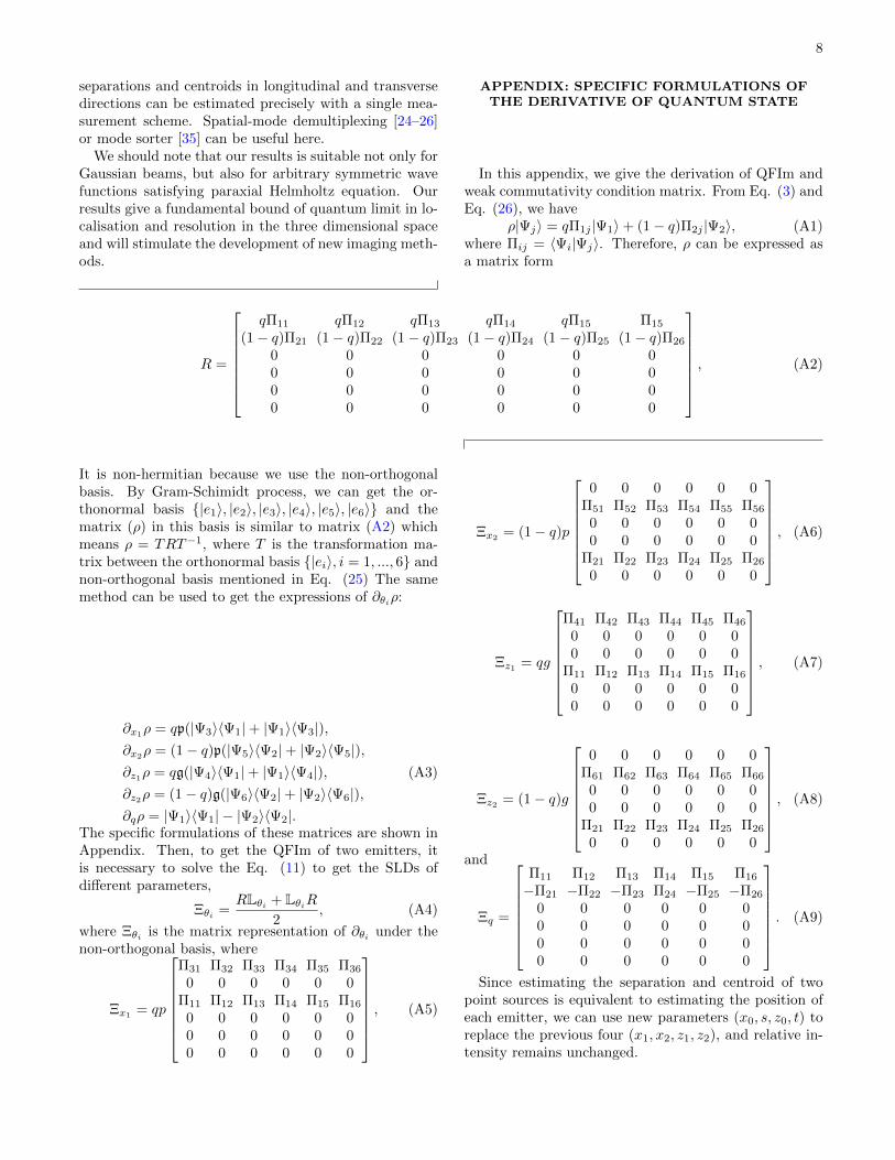
APPENDIX: SPECIFIC FORMULATIONS OFTHE DERIVATIVE OF QUANTUM STATE

In this appendix, we give the derivation of QFIm andweak commutativity condition matrix. From Eq. (3) andEq. (26), we have

ρ|Ψj〉 = qΠ1j |Ψ1〉+ (1− q)Π2j |Ψ2〉, (A1)where Πij = 〈Ψi|Ψj〉. Therefore, ρ can be expressed asa matrix form

R =

qΠ11 qΠ12 qΠ13 qΠ14 qΠ15 Π15

(1− q)Π21 (1− q)Π22 (1− q)Π23 (1− q)Π24 (1− q)Π25 (1− q)Π26

0 0 0 0 0 00 0 0 0 0 00 0 0 0 0 00 0 0 0 0 0

, (A2)

It is non-hermitian because we use the non-orthogonalbasis. By Gram-Schimidt process, we can get the or-thonormal basis {|e1〉, |e2〉, |e3〉, |e4〉, |e5〉, |e6〉} and thematrix (ρ) in this basis is similar to matrix (A2) whichmeans ρ = TRT−1, where T is the transformation ma-trix between the orthonormal basis {|ei〉, i = 1, ..., 6} andnon-orthogonal basis mentioned in Eq. (25) The samemethod can be used to get the expressions of ∂θiρ:

∂x1ρ = qp(|Ψ3〉〈Ψ1|+ |Ψ1〉〈Ψ3|),

∂x2ρ = (1− q)p(|Ψ5〉〈Ψ2|+ |Ψ2〉〈Ψ5|),

∂z1ρ = qg(|Ψ4〉〈Ψ1|+ |Ψ1〉〈Ψ4|),∂z2ρ = (1− q)g(|Ψ6〉〈Ψ2|+ |Ψ2〉〈Ψ6|),∂qρ = |Ψ1〉〈Ψ1| − |Ψ2〉〈Ψ2|.

(A3)

The specific formulations of these matrices are shown inAppendix. Then, to get the QFIm of two emitters, itis necessary to solve the Eq. (11) to get the SLDs ofdifferent parameters,

Ξθi =RLθi + LθiR

2, (A4)

where Ξθi is the matrix representation of ∂θi under thenon-orthogonal basis, where

Ξx1= qp

Π31 Π32 Π33 Π34 Π35 Π36

0 0 0 0 0 0Π11 Π12 Π13 Π14 Π15 Π16

0 0 0 0 0 00 0 0 0 0 00 0 0 0 0 0

, (A5)

Ξx2= (1− q)p

0 0 0 0 0 0

Π51 Π52 Π53 Π54 Π55 Π56

0 0 0 0 0 00 0 0 0 0 0

Π21 Π22 Π23 Π24 Π25 Π26

0 0 0 0 0 0

, (A6)

Ξz1 = qg

Π41 Π42 Π43 Π44 Π45 Π46

0 0 0 0 0 00 0 0 0 0 0

Π11 Π12 Π13 Π14 Π15 Π16

0 0 0 0 0 00 0 0 0 0 0

, (A7)

Ξz2 = (1− q)g

0 0 0 0 0 0

Π61 Π62 Π63 Π64 Π65 Π66

0 0 0 0 0 00 0 0 0 0 0

Π21 Π22 Π23 Π24 Π25 Π26

0 0 0 0 0 0

, (A8)

and

Ξq =

Π11 Π12 Π13 Π14 Π15 Π16

−Π21 −Π22 −Π23 Π24 −Π25 −Π26

0 0 0 0 0 00 0 0 0 0 00 0 0 0 0 00 0 0 0 0 0

. (A9)

Since estimating the separation and centroid of twopoint sources is equivalent to estimating the position ofeach emitter, we can use new parameters (x0, s, z0, t) toreplace the previous four (x1, x2, z1, z2), and relative in-tensity remains unchanged.

9

θ1 = x0 =x2 + x1

2, θ2 = s = x2 − x1,

θ3 = z0 =z2 + z1

2, θ4 = t = z2 − z1,

θ5 = q.

(A10)

The relation between the SLDs of the new parameterswith respect to the old ones can be written as

Lx0

LsLz0LtLq

=

1 1 0 0 0− 1

212 0 0 0

0 0 1 1 00 0 − 1

212 0

0 0 0 0 1

Lx1

Lx2

Lz1Lz2Lq

. (A11)

Now, we take the SLD of x0 as an example to show therelation in Eq. (A11). The parameter x0 has the samegenerator p with x1 and x2. According to Eq. (3) and Eq.(26), ∂x1

ρ = iq [|Ψ1〉〈Ψ1|, p], ∂x2ρ = i(1− q) [|Ψ2〉〈Ψ2|, p]

and

|Ψ1〉 = exp(−iGz1 − ipx1

)|Ψ〉

= exp(−iGz1 − ip(x0 −

s

2))|Ψ〉,

|Ψ2〉 = exp(−iGz2 − ipx2

)|Ψ〉

= exp(−iGz2 − ip(x0 +

s

2))|Ψ〉.

(A12)

So ∂x0|Ψ1〉 = ∂x1

|Ψ1〉 and ∂x0|Ψ2〉 = ∂x2

|Ψ2〉, then wecan get

∂x0ρ = i [ρ, p] = ∂x1

ρ+ ∂x2ρ. (A13)

From the definition of SLD Eq. (11) and Eq. (A13), wecan show that

Lx0 = Lx1+ Lx2

. (1)

The other relations of SLDs can be derived in a similarway.

Next, QFIm and weak commutativity condition matrixcan be derivated from Eq. (10) and Eq. (12)

[Q (ρ)]µν + i [Γ (ρ)]µν = Tr [ρLµLν ] , (A14)where

Tr [ρLµLν ] = Tr[TRT−1TLµT−1TLνT−1]

= Tr[RLµLν ].(A15)

Note added. we are aware of the related independentwork in [55].

Funding. This work was supported by the Na-tional Key Research and Development Program of China(Grant Nos. 2017YFA0303703 and 2018YFA030602) andthe National Natural Science Foundation of China (GrantNos. 91836303, 61975077, 61490711 and 11690032) andFundamental Research Funds for the CentralUniversities(Grant No. 020214380068).

Disclosures. The authors declare no conflicts of in-terest.

∗ lijian.zhang@nju.edu.cn[1] Max Born and Emil Wolf. Principles of optics, 7th (ex-

panded) edition. United Kingdom: Press Syndicate of theUniversity of Cambridge, 461, 1999.

[2] Lord Rayleigh. Xxxi. investigations in optics, with specialreference to the spectroscope. The London, Edinburgh,and Dublin Philosophical Magazine and Journal of Sci-ence, 8(49):261–274, 1879.

[3] Stefan W. Hell and Jan Wichmann. Breaking the diffrac-tion resolution limit by stimulated emission: stimulated-emission-depletion fluorescence microscopy. Opt. Lett.,19(11):780–782, Jun 1994.

[4] Rainer Heintzmann, Thomas M. Jovin, and ChristophCremer. Saturated patterned excitation microscopy—aconcept for optical resolution improvement. J. Opt. Soc.Am. A, 19(8):1599–1609, Aug 2002.

[5] Mats G. L. Gustafsson. Nonlinear structured-illumination microscopy: Wide-field fluorescence imagingwith theoretically unlimited resolution. Proceedings ofthe National Academy of Sciences, 102(37):13081–13086,2005.

[6] Michael J. Rust, Mark Bates, and Xiaowei Zhuang. Sub-diffraction-limit imaging by stochastic optical reconstruc-tion microscopy (storm). Nature Methods, 3(10):793–796,2006.

[7] Eric Betzig, George H. Patterson, Rachid Sougrat,O. Wolf Lindwasser, Scott Olenych, Juan S. Bonifacino,Michael W. Davidson, Jennifer Lippincott-Schwartz, andHarald F. Hess. Imaging intracellular fluorescent proteinsat nanometer resolution. Science, 313(5793):1642–1645,2006.

[8] L. A. Howard, G. G. Gillett, M. E. Pearce, R. A. Abra-hao, T. J. Weinhold, P. Kok, and A. G. White. Optimalimaging of remote bodies using quantum detectors. Phys.Rev. Lett., 123:143604, Sep 2019.

[9] Magdalena Szczykulska, Tillmann Baumgratz, and Ani-mesh Datta. Multi-parameter quantum metrology. Ad-vances in Physics: X, 1(4):621–639, 2016.

[10] K Matsumoto. A new approach to the cramer-rao-typebound of the pure-state model. Journal of Physics A:Mathematical and General, 35(13):3111–3123, mar 2002.

[11] Luca Pezze, Mario A. Ciampini, Nicolo Spagnolo, Pe-ter C. Humphreys, Animesh Datta, Ian A. Walmsley,Marco Barbieri, Fabio Sciarrino, and Augusto Smerzi.Optimal measurements for simultaneous quantum esti-mation of multiple phases. Phys. Rev. Lett., 119:130504,Sep 2017.

[12] O. Pinel, P. Jian, N. Treps, C. Fabre, and D. Braun.Quantum parameter estimation using general single-mode gaussian states. Phys. Rev. A, 88:040102, Oct 2013.

[13] Mihai D Vidrighin, Gaia Donati, Marco G Genoni, Xian-Min Jin, W Steven Kolthammer, MS Kim, AnimeshDatta, Marco Barbieri, and Ian A Walmsley. Joint esti-mation of phase and phase diffusion for quantum metrol-ogy. Nature communications, 5:3532, 2014.

[14] Peter C. Humphreys, Marco Barbieri, Animesh Datta,and Ian A. Walmsley. Quantum enhanced multiple phase

10

estimation. Phys. Rev. Lett., 111:070403, Aug 2013.[15] Philip J. D. Crowley, Animesh Datta, Marco Barbieri,

and I. A. Walmsley. Tradeoff in simultaneous quantum-limited phase and loss estimation in interferometry. Phys.Rev. A, 89:023845, Feb 2014.

[16] Sammy Ragy, Marcin Jarzyna, and Rafa l Demkowicz-Dobrzanski. Compatibility in multiparameter quantummetrology. Phys. Rev. A, 94:052108, Nov 2016.

[17] Samuel L. Braunstein and Carlton M. Caves. Statisticaldistance and the geometry of quantum states. Phys. Rev.Lett., 72:3439–3443, May 1994.

[18] Vittorio Giovannetti, Seth Lloyd, and Lorenzo Mac-cone. Advances in quantum metrology. Nature photonics,5(4):222, 2011.

[19] Vittorio Giovannetti, Seth Lloyd, and Lorenzo Maccone.Quantum metrology. Phys. Rev. Lett., 96:010401, Jan2006.

[20] Jing Liu, Haidong Yuan, Xiao-Ming Lu, and XiaoguangWang. Quantum fisher information matrix and multipa-rameter estimation. Journal of Physics A: Mathematicaland Theoretical, 53(2):023001, dec 2019.

[21] Haidong Yuan and Chi-Hang Fred Fung. Quantummetrology matrix. Phys. Rev. A, 96:012310, Jul 2017.

[22] Yu Chen and Haidong Yuan. Maximal quantum fisher in-formation matrix. New Journal of Physics, 19(6):063023,jun 2017.

[23] Mankei Tsang, Ranjith Nair, and Xiao-Ming Lu. Quan-tum theory of superresolution for two incoherent opticalpoint sources. Phys. Rev. X, 6:031033, Aug 2016.

[24] Martin Paur, Bohumil Stoklasa, Zdenek Hradil, Luis L.Sanchez-Soto, and Jaroslav Rehacek. Achieving the ul-timate optical resolution. Optica, 3(10):1144–1147, Oct2016.

[25] Mankei Tsang. Subdiffraction incoherent optical imag-ing via spatial-mode demultiplexing: Semiclassical treat-ment. Phys. Rev. A, 97:023830, Feb 2018.

[26] Mankei Tsang. Subdiffraction incoherent optical imag-ing via spatial-mode demultiplexing. New Journal ofPhysics, 19(2):023054, feb 2017.

[27] Weng-Kian Tham, Hugo Ferretti, and Aephraim M.Steinberg. Beating rayleigh’s curse by imaging usingphase information. Phys. Rev. Lett., 118:070801, Feb2017.

[28] Kent A G Bonsma-Fisher, Weng-Kian Tham, Hugo Fer-retti, and Aephraim M Steinberg. Realistic sub-rayleighimaging with phase-sensitive measurements. New Jour-nal of Physics, 21(9):093010, sep 2019.

[29] Michael R Grace, Zachary Dutton, Amit Ashok, andSaikat Guha. Approaching quantum limited super-resolution imaging without prior knowledge of the objectlocation. arXiv preprint arXiv:1908.01996, 2019.

[30] Micha l Parniak, Sebastian Borowka, Kajetan Boroszko,Wojciech Wasilewski, Konrad Banaszek, and Rafa lDemkowicz-Dobrzanski. Beating the rayleigh limit usingtwo-photon interference. Phys. Rev. Lett., 121:250503,Dec 2018.

[31] J. Rehacek, Z. Hradil, B. Stoklasa, M. Paur, J. Grover,A. Krzic, and L. L. Sanchez-Soto. Multiparameter quan-tum metrology of incoherent point sources: Towards real-istic superresolution. Phys. Rev. A, 96:062107, Dec 2017.

[32] J. Rehacek, Z. Hradil, D. Koutny, J. Grover, A. Krzic,and L. L. Sanchez-Soto. Optimal measurements for quan-tum spatial superresolution. Phys. Rev. A, 98:012103, Jul2018.

[33] Sudhakar Prasad. Quantum limited super-resolution ofan unequal-brightness source pair in three dimensions.Physica Scripta, 95(5):054004, mar 2020.

[34] Evangelia Bisketzi, Dominic Branford, and AnimeshDatta. Quantum limits of localisation microscopy. NewJournal of Physics, 21(12):123032, dec 2019.

[35] Yiyu Zhou, Jing Yang, Jeremy D. Hassett, Seyed Mo-hammad Hashemi Rafsanjani, Mohammad Mirhosseini,A. Nick Vamivakas, Andrew N. Jordan, Zhimin Shi, andRobert W. Boyd. Quantum-limited estimation of the ax-ial separation of two incoherent point sources. Optica,6(5):534–541, May 2019.

[36] Zhixian Yu and Sudhakar Prasad. Quantum limited su-perresolution of an incoherent source pair in three dimen-sions. Phys. Rev. Lett., 121:180504, Oct 2018.

[37] Sudhakar Prasad and Zhixian Yu. Quantum-limited su-perlocalization and superresolution of a source pair inthree dimensions. Phys. Rev. A, 99:022116, Feb 2019.

[38] Carmine Napoli, Samanta Piano, Richard Leach, Ger-ardo Adesso, and Tommaso Tufarelli. Towards superres-olution surface metrology: Quantum estimation of angu-lar and axial separations. Phys. Rev. Lett., 122:140505,Apr 2019.

[39] Mikael P. Backlund, Yoav Shechtman, and Ronald L.Walsworth. Fundamental precision bounds for three-dimensional optical localization microscopy with poissonstatistics. Phys. Rev. Lett., 121:023904, Jul 2018.

[40] Walker Larson and Bahaa E. A. Saleh. Resurgence ofrayleigh’s curse in the presence of partial coherence. Op-tica, 5(11):1382–1389, Nov 2018.

[41] Mankei Tsang and Ranjith Nair. Resurgence of rayleigh’scurse in the presence of partial coherence: comment. Op-tica, 6(4):400–401, Apr 2019.

[42] Walker Larson and Bahaa E. A. Saleh. Resurgence ofrayleigh’s curse in the presence of partial coherence: re-ply. Optica, 6(4):402–403, Apr 2019.

[43] Zdenek Hradil, Jaroslav Rehacek, Luis Sanchez-Soto, andBerthold-Georg Englert. Quantum fisher informationwith coherence. Optica, 6(11):1437–1440, Nov 2019.

[44] Yoav Shechtman, Steffen J. Sahl, Adam S. Backer, andW. E. Moerner. Optimal point spread function designfor 3d imaging. Phys. Rev. Lett., 113:133902, Sep 2014.

[45] Elias Nehme, Boris Ferdman, Lucien E Weiss, Tal Naor,Daniel Freedman, Tomer Michaeli, and Yoav Shechtman.Learning an optimal psf-pair for ultra-dense 3d localiza-tion microscopy. arXiv preprint arXiv:2009.14303, 2020.

[46] J. Rehacek, M. Paur, B. Stoklasa, D. Koutny, Z. Hradil,and L. L. Sanchez-Soto. Intensity-based axial localizationat the quantum limit. Phys. Rev. Lett., 123:193601, Nov2019.

[47] Martin Paur, Bohumil Stoklasa, Jai Grover, AndrejKrzic, Luis L. Sanchez-Soto, Zdenek Hradil, and JaroslavRehacek. Tempering rayleigh’s curse with psf shaping.Optica, 5(10):1177–1180, Oct 2018.

[48] D Koutny, Z Hradil, J Rehacek, and L L Sanchez-Soto.Axial superlocalization with vortex beams. Quantum Sci-ence and Technology, 6(2):025021, mar 2021.

[49] Carl W Helstrom and Carl W Helstrom. Quantum de-tection and estimation theory, volume 3. Academic pressNew York, 1976.

[50] Alexander S Holevo. Probabilistic and statistical aspectsof quantum theory, volume 1. Springer Science & Busi-ness Media, 2011.

[51] Angelo Carollo, Bernardo Spagnolo, Alexander A

11

Dubkov, and Davide Valenti. On quantumness in multi-parameter quantum estimation. Journal of StatisticalMechanics: Theory and Experiment, 2019(9):094010, sep2019.

[52] Mankei Tsang, Francesco Albarelli, and Animesh Datta.Quantum semiparametric estimation. Phys. Rev. X,10:031023, Jul 2020.

[53] Chandan Datta, Marcin Jarzyna, Yink Loong Len, Karol Lukanowski, Jan Ko lodynski, and Konrad Banaszek.Sub-rayleigh resolution of incoherent sources by array ho-

modyning. arXiv preprint arXiv:2005.08693, 2020.[54] Yink Loong Len, Chandan Datta, MichaA,Parniak, and

Konrad Banaszek. Resolution limits of spatial mode de-multiplexing with noisy detection. International Journalof Quantum Information, 18(01):1941015, 2020.

[55] Lukas J Fiderer, Tommaso Tufarelli, Samanta Piano, andGerardo Adesso. General expressions for the quantumfisher information matrix with applications to discretequantum imaging. arXiv preprint arXiv:2012.01572,2020.