quantum field theory - university of cambridge · 2016-10-12 · there are many reasons to study...

Cambrige Part III MathsMichaelmas 2015

Quantum Field Theory

based on a course given by written up byMalcolm Perry Josh Kirklin

Please send errors and suggestions to [email protected].

Contents1 Introduction 2

1.1 Why study QFT? . . . . . . . . . . . . . . . . . . . . . . . . . . . . . . . . . . . . . 21.2 Special relativity . . . . . . . . . . . . . . . . . . . . . . . . . . . . . . . . . . . . . 21.3 Quantum mechanics . . . . . . . . . . . . . . . . . . . . . . . . . . . . . . . . . . . 5

2 Scalar Fields 62.1 Classical scalar fields . . . . . . . . . . . . . . . . . . . . . . . . . . . . . . . . . . . 62.2 Quantisation . . . . . . . . . . . . . . . . . . . . . . . . . . . . . . . . . . . . . . . 72.3 Plane wave expansion . . . . . . . . . . . . . . . . . . . . . . . . . . . . . . . . . . 92.4 The quantum Hamiltonian . . . . . . . . . . . . . . . . . . . . . . . . . . . . . . . . 112.5 Heisenberg picture . . . . . . . . . . . . . . . . . . . . . . . . . . . . . . . . . . . . 132.6 The Feynman propagator . . . . . . . . . . . . . . . . . . . . . . . . . . . . . . . . 142.7 Consistency with causality . . . . . . . . . . . . . . . . . . . . . . . . . . . . . . . . 17

3 Spinor Fields 193.1 Dirac equation . . . . . . . . . . . . . . . . . . . . . . . . . . . . . . . . . . . . . . 193.2 Plane wave spinors . . . . . . . . . . . . . . . . . . . . . . . . . . . . . . . . . . . . 223.3 Quantise that sucker . . . . . . . . . . . . . . . . . . . . . . . . . . . . . . . . . . . 243.4 Hamiltonian operator . . . . . . . . . . . . . . . . . . . . . . . . . . . . . . . . . . 273.5 Dirac current . . . . . . . . . . . . . . . . . . . . . . . . . . . . . . . . . . . . . . . 273.6 Propagator for the Dirac field . . . . . . . . . . . . . . . . . . . . . . . . . . . . . . 28

4 Maxwell Field 294.1 Gauge invariance . . . . . . . . . . . . . . . . . . . . . . . . . . . . . . . . . . . . . 304.2 Quantisation . . . . . . . . . . . . . . . . . . . . . . . . . . . . . . . . . . . . . . . 31

5 Path Integrals and Interaction 345.1 Quantum mechanics . . . . . . . . . . . . . . . . . . . . . . . . . . . . . . . . . . . 345.2 Fields . . . . . . . . . . . . . . . . . . . . . . . . . . . . . . . . . . . . . . . . . . . 365.3 Interaction . . . . . . . . . . . . . . . . . . . . . . . . . . . . . . . . . . . . . . . . 385.4 φ3 theory . . . . . . . . . . . . . . . . . . . . . . . . . . . . . . . . . . . . . . . . . 38

– 1 –

[email protected]

1 Introduction 1 Introduction

5.5 φ4 theory . . . . . . . . . . . . . . . . . . . . . . . . . . . . . . . . . . . . . . . . . 425.6 Higher loops . . . . . . . . . . . . . . . . . . . . . . . . . . . . . . . . . . . . . . . . 445.7 Free fermions . . . . . . . . . . . . . . . . . . . . . . . . . . . . . . . . . . . . . . . 455.8 Quantum electrodynamics . . . . . . . . . . . . . . . . . . . . . . . . . . . . . . . . 485.9 Complete Feynman rules . . . . . . . . . . . . . . . . . . . . . . . . . . . . . . . . . 48

1 IntroductionIn these notes we will use natural units: ~ = c = 1, [L] = [T ] = [M ]−1.

1.1 Why study QFT?There are many reasons to study Quantum Field Theory.

• QFT provides a way to unify special relativity with quantum mechanics.

• Using QFT, we can understand what spin is and how it works. For example we can deducethe reason why bosons have Bose-Einstein statistics, and fermions have Fermi-Dirac statistics.

• QFT enables us to explain why particles exist, and furthermore why they can morph intodifferent forms over time. In other words, we can analyse the reactions between variousspecies of particle, for example electron positron annihilation: e+e− → 2γ.

• The “Rayleigh-Jeans catastrophe” is a problem that arises in dealing with the electromagneticfield. In simple terms the problem is that a certain law predicts divergences at high energies.With QFT we can solve this problem and other more general ultraviolet divergences.

• QFT provides a theoretical framework for describing and studying all fundamental processes1.The best theory for our world that we have today is the Standard Model, which has experi-mentally been found to accurately describe electromagnetic, weak and strong interactions tofive decimal places.

1.2 Special relativity

Definition. Minkowski spacetime R3,1 is a four-dimensional space equipped with the Minkowskimetric η = diag(−1, 1, 1, 1).

The geometry of Minkowski spacetime is described by its line element:

ds2 = ηab dxa dxb = −dt2 + dx2 + dy2 + dz2

In rough terms, ds is the “distance” between the infinitesimally close points (t, x, y, z) and (t +dt , x+ dx , y + dy , z + dz).Vectors in Minkowski space can be classified into five different types, depending on their relation tothe lightcone, i.e. the locus of all points xa with ηabx

axb = x · x = |x|2 = 0.

1Except of course for gravitation. For that we require something else; String Theory for instance.

– 2 –

1 Introduction 1.2 Special relativity

1

2

3

4

5

1. Future directed null vectors.

2. Past directed null vectors.

3. Future directed timelike vectors.

4. Past directed timelike vectors.

5. Spacelike vectors.

Definition. A Lorentz transformation is a transformation x → x′ = Λx between inertialframes such that ΛᵀηΛ = η. We say that Λ preserves the Minkowski metric.

Example. Suppose one wants to transform a rest frame to one moving at velocity v in the(positive) x-direction. Then we can use the following Lorentz transformation:

t→ t′ = t− vx√1− v2

x→ x′ = x− vt√1− v2

y → y′ = y

z → z′ = z

The set of all Lorentz transformations equipped with matrix multiplication form a group which wecall the Lorentz group SO(3, 1):

• Matrix multiplication is associative.

• Suppose Λ,Λ′ ∈ SO(3, 1). Then ΛΛ′ᵀηΛΛ′ = Λ′ᵀΛᵀηΛΛ′ = Λ′ᵀηΛ′ = η, so ΛΛ′ ∈ SO(3, 1),i.e. SO(3, 1) is closed.

• The matrix identity 1 is an element of SO(3, 1).

• Suppose Λ ∈ SO(3, 1). Then taking the determinant of both sides of ΛᵀηΛ = η we obtain−(det Λ)2 = −1, so det Λ 6= 0 i.e. Λ is invertible. Moreover, if we left-multiply by Λᵀ−1 andright-multiply by Λ−1 we obtain η = Λᵀ−1ηΛ−1, so Λ−1 ∈ SO(3, 1).

The Lorentz group contains spatial rotations. For example, a rotation of θ about the x-axis is givenby:

Λ =

1

cos θ − sin θsin θ cos θ

1

More generally, a rotation of θ about the direction given by a 3D unit vector ni can be written:

Λ =(

1R

)where Rij = cos θδij + ninj(1− cos θ)− εijknk sin θ

– 3 –

1 Introduction 1.2 Special relativity

A Lorentz boost is a shift in velocity between frames. The Lorentz boost with velocity shift givenby a 3D vector vi can be written:

Λ =(

γ −γvi−γvj δij + γ2

1+γ vivj

)where γ = (1− vivi)−

12

Definition. A proper Lorentz transformation Λ has det Λ = 1. An improper Lorentz transfor-mation Λ has det Λ = −1.

Proper Lorentz transformations are continuously connected to the identity. Under a proper Lorentztransformation, the type (i.e. spacelike, future directed timelike, etc) of a vector is invariant. Bothrotations and boosts are proper.There are two types of improper Lorentz transformations:

• Parity transformation: ~x→ −~x.

• Time reversal: t→ −t.

Time reversal maps

futurepast

directed vectors to

past

future

directed vectors.

The action of a Lorentz transform on spacetime co-ordinates is to take xa → xa = Λabxb, but otherobjects transform in other ways.

Definition. An X-valued scalar field is a field in spacetime S : R3,1 → X that is invariantunder Lorentz transformations:

S(x)→ S(x) = S(Λx)

Definition. An X-valued covariant vector field is a set of fields in spacetime V a : R3,1 → Xthat transform just like co-ordinates under Lorentz transforms:

V a(x)→ V a(x) = ΛabV b(Λx)

In this course we will deal usually with fields that are R or C-valued.Two vector fields can be combined into a scalar field by taking their inner product.A useful convention is to swap the positions of indices upstairs or downstairs using the metric η.E.g. Wa = ηabW

b where W b is a covariant vector. Wa is a contravariant vector and is dual to W b.We also define ηab = (η−1)ab.In index notation, we have for any Lorentz transformation Λ:

ΛacΛbdηab = ηcd

Now pre-multiply by the inverse of Λ:

(Λ−1)ceΛac︸︷︷︸=δae

ηab = (Λ−1)ceηcd =⇒ Λbdηeb = (Λ−1)ceηcd

– 4 –

1 Introduction 1.3 Quantum mechanics

Now post-multiply by an η:

Λbdηebηdf = (Λ−1)ceηcdηdf = (Λ−1)fe

So, since we are adopting the convention that any index can be raised or lowered using η, we have:

(Λ−1)fe = Λ fe i.e. Λ−1 = Λᵀ

We can deduce how a contravariant tensor transforms:

Wa → Wa = ηabWb = ηabΛbcW c = ηabη

bdΛ ed ηecW

c = Λ ea We

Definition. An X-valued tensor field of rank (n,m) is a set of fields T a1...anb1...bm

: R3,1 → Xthat transform with n covariant indices and m contravariant indices, i.e.:

T a1...b1...

(x)→ T c1...d1...

(x) = Λc1a1 · · ·Λ

b1d1· · ·T a1...

b1...(Λx)

Definition. A symmetry of Minkowski spacetime is a transformation that leaves the lineelement invariant. The group of symmetries of Minkowski spacetime is called the Poincaregroup.

The Poincare group includes Lorentz transformations as well as spacetime translations. In fact it isa 10-dimensional group:

• 3 spatial rotations

• 3 Lorentz boosts

• 3 spatial translations

• 1 time translation

These 10 transformations correspond to the 10 Killing vectors of Minkowski space.In Minkowski space in Cartesian coordinates the differential operators ∂a = ∂

∂xa map tensors oftype (n,m) to tensors of type (n,m+ 1).

1.3 Quantum mechanicsWhen we quantise a classical theory, we convert classical observables into Hermitian operators. Forexample for a one particle system, we have an energy operator E = i ∂∂t and a momentum operator~p = −i∇. Classically, energy and spatial momentum are combined into 4-momentum p given by:

pa = (energy, spatial momentum) or equivalently pa = (−energy, spatial momentum)

Thus we can define a 4-momentum operator pa = −i∂a. In non-relativistic quantum mechanics, piand xj obey the Heisenberg algebra:

[pi, xj ] = −iδjiTo make this relativistic, we simply include time coordinates, so we take pi → pa and xj → pb:

[pa, xb] = −iδba (or [pa, xb] = −iηab etc.)

– 5 –

2 Scalar Fields 2 Scalar Fields

Classically, we define the angular momentum with Li = (~x× ~y)i = εijkxjpk. But now we encounterproblems in translating to relativistic quantum mechanics. Classically, the ordering of xj , pk doesnot matter, but quantumly the ordering of xj , pk does. Furthermore, εijk is a 3D alternating symbol,which does not fit with our 4D Minkowski spacetime. The way we get around these problems is toinstead think of angular momentum as an antisymmetric tensor Lij = xipj − xjpi, or in relativisticform Lab = xapb − paxb. Note that xa and pb only don’t commute if a = b, and because Lab isantisymmetric, we need not worry about that case. So after quantisation we obtain:

Lab = −ixa∂b + ixb∂a

It is not hard to show that:

[Lab, Lcd] = i(Ladηbc − Lacηbd − Lbdηac + Lbcηad)

This is exactly the bracket structure for the Lie algebra of the Lorentz group L(SO(3, 1)), so thisshows that Lab forms a representation of L(SO(3, 1)).

2 Scalar Fields2.1 Classical scalar fieldsConsider fields φ(x, t) that are eigenstates of the momentum operator −i∂a. It is easy to see thatthese are the plane wave states φ = eikax

a with eigenvalue ka. If ka is a physical momentum, as itshould be, then it is a contravariant vector. Thus kaxa is a scalar and so is φ.Fourier transforms give a way of moving between spatial co-ordinates and relativistic momenta,φ(x)→ φ(p):

φ(p) =∫

d4xφ(x)e−ipaxa

where d4x = d3x dt =∏a dxa and the integral is taken over all of spacetime. This has an exact

inverse φ(p)→ φ(x):φ(x) = 1

(2π)4

∫d4p φ(p)eipaxa

where d4p = d3p dp0 = d3pdE =∏a dpa and the integral is taken over all 4-momenta.

The Fourier transform of a plane wave state is given by a delta function:∫d4x eikbx

be−ipax

a =∫

d4x ei(k0−p0)t+i(~k−~p)·~x = (2π)4δ(4)(k − p)

In special relativity, the rest mass m of a particle is given by papa = −E2 + p2 = −m2. If we writethis in terms of the momentum operator, we obtain the Klein-Gordon equation:

(− +m2)φ = 0

where = ηab∂a∂b = ∂2

∂t2 −∇2 is the relativistic d’Alembertian or wave operator. We will want the

Klein-Gordon equation to be the equation of motion for our field, so it is natural to ask: is there aLagrangian action to to reproduce it? The answer is yes, and the action is the Klein-Gordon action:

I =∫

d4x

(−1

2ηab∂aφ∂bφ−

12m

2φ2)

– 6 –

2 Scalar Fields 2.2 Quantisation

To verify that this is the case, let’s vary I with regard to φ:

δI =∫

d4x(−ηab∂a δφ ∂aφ−m2φ δφ

)=∫

d4x(ηab∂a∂bφ−m2φ

)︸︷︷︸

Klein-Gordon

δφ+∫

dΣa (δφ ∂aφ)︸︷︷︸boundary term

where we reach the second line by partial integration. In this course we will assume that all fieldsgo to zero sufficiently quickly as we approach infinity, so the boundary term vanishes. Thus, sinceδφ is arbitrary, in order to satisfy δI = 0 we must have ηab∂a∂bφ−m2φ = 0, i.e. the Klein-Gordonequation must hold.

2.2 QuantisationLets summarise how classical dynamics progresses through the Hamiltonian formalism to quantummechanics. In normal classical dynamics we have a (usually finite) set of generalised coordinates qi,labelled by i. We define the generalised momenta πi congugate to each coordinate qi by:

πi = ∂L

∂qi

We can solve this equation for qi as a function of the πj and qk. We then define the Hamiltonian by:

H(πi, qi) =∑i

πiqi(πj , qk)− L

Given any observable X(π, q), its time evolution is given by:

X = X,HP

where the braced quantity is the Poisson bracket, defined by:

X,Y P =∑i

∂X

∂qi

∂Y

∂πi− ∂X

∂πi

∂Y

∂qi

Note that we have qi, πjP = δij .To quantise, we must “deform” the classical system by replacing q, π and other observables byHermitian operators, and by replacing all Poisson brackets by a commutator:

X,Y P → −i[X, Y ]

For example, qi, πjP = δij becomes [qi, πj ] = i~δij .Now return to the scalar field.

Definition. The functional derivative δFδf of a functional F [f ] is defined in the following way:

δF [f(x)]δf(y) = ∂

∂εF [f(x) + εδ(x− y)]

∣∣∣∣ε=0

where the delta function has the appropriate dimensionality.

– 7 –

2 Scalar Fields 2.2 Quantisation

Functional derivatives follow all of the normal rules of derivatives (e.g. the chain rule and productrule).For example, for the Klein-Gordon action we have:

δI

δφ(x) = ηab∂a∂bφ(x)−m2φ(x)

We view the action I as an integral over all time of a Lagrangian L(φ, φ):

I =∫

dt L(φ, φ) where L(φ, φ) =∫

d3x

(12 φ

2 − 12(∇φ)2 − 1

2m2φ2

)In field theory, we have an infinite continuum of generalised co-ordinates φ(x) labelled by pointsin space x. In order to account for this, to produce a Hamiltonian formalism we use functionalderivatives instead of partial derivatives.

Definition. The momentum conjugate to a particular field φ(x) with a Lagrangian L is givenby:

π(x) = δL

δφ(x)

For a scalar field obeying the Klein-Gordon equation, we have π(x) = φ(x). The Hamiltonian H isgiven by:

H =∫

d3xπ(x)φ(x)− L

For a scalar field obeying the Klein-Gordon equation, this becomes:

H =∫

d3xπ(x)φ(x)− 12 φ

2 + 12(∇φ)2 + 1

2m2φ2

=∫

d3x12π

2 + 12(∇φ)2 + 1

2m2φ2

The Poisson bracket also adapts to include functional derivatives and integrals. For any observableO(x)−O(φ(x), π(x)), we have:

O(x) = O,HP (x)

=∫

d3zδO(x)δφ(z)

δH

δπ(z) −δO(x)δπ(z)

δH

δφ(z)

For example:

φ(x) = φ(x), HP =∫

d3zδφ(x)δφ(z)︸︷︷︸

=δ(3)(x−z)

=∫

d3yπ(y)δ(3)(y−z)=π(z)︷︸︸︷δH

δπ(z) −δφ(x)δπ(z)︸︷︷︸

=0

δH

δφ(z)

=∫

d3z δ(3)(x− z)π(z)

= π(x)

– 8 –

2 Scalar Fields 2.3 Plane wave expansion

as expected. We can also now calculate π:

π(x) = π(x), HP =∫

d3zδπ(x)δφ(z)︸︷︷︸

=0

δH

δπ(z) −δπ(x)δπ(z)︸︷︷︸

=δ(3)(x−z)

=∫

d3ym2φ(x)δ(3)(x−z)+∇φ(x)·∇δ(3)(x−z)=m2φ(z)−∇2φ(z)︷︸︸︷δH

δφ(z)

=∫

d3z δ(3)(x− z)(−m2φ(z) +∇2φ(z)

= −m2φ(x) +∇2φ(x)

So our Hamiltonian equations of motion are φ = π and π = −m2φ+∇2φ. Combining these, wehave φ = π = −m2φ+∇2φ, or written another way φ−m2φ = 0 i.e. we recover the Klein-Gordonequation.So let’s now quantise the scalar field. We replace φ(x), π(x) with operators φ(x), π(x). These arenot wavefunctions - they are operators labelled by a position in space. In the classical case we have:

φ(x), π(y) = δ(3)(x− z), φ(x), φ(y)P = π(x), φ(y)P = 0

so we translate this into a set of commutation relation:

[φ(x), π(y)] = iδ(3)(x− y), [φ(x), φ(y)] = [π(x), π(y)] = 0 (∗)

From now on we will drop the hats in notation; whether we are referring to quantum operators orclassical variables should be obvious from context.Recall that in quantum physics we can take one of two viewpoints:

Schrodinger picture: States are time-dependent, and operators are time-independent.

Heisenberg picture: States are time-independent, and operators are time-dependent.

We can move between these two pictures by using a unitary transformation, the time evolutionoperator e−iHt where H = i ∂∂t . Let |s〉 be a state and O an operator, and let subscripts S and Hdenote the Schrodinger and Heisenberg pictures respectively. Then we have:

|s(t)〉S = e−iHt |s〉HOS = e−iHtOHe+iHt

Note that (∗) are Schrodinger picture equations, since φ and π appear to be time-independent. Fornow, we will continue to initially work in the Schrodinger picture.

2.3 Plane wave expansionLets expand the operator φ(x) in terms of a plane wave basis:

φ(x) =∑

pape

ip·x + a†pe−ip·x

Here the ap are operators. We have chosen the coefficient of e−ip·x to be a†p in order to keep φ(x)Hermitian.p is a continuous variable and so the sum

∑p really ought to be some kind of integral. We have

some freedom of choice here in the measure we use for this integral. This is not a problem, as any

– 9 –

2 Scalar Fields 2.3 Plane wave expansion

differences in measure would result in correspondingly different definitions of the operators ap - theresulting expressions for φ(x) and other quantities would be equivalent. The most common choiceis the following: ∑

p=∫ d3p

(2π)31

2Ep(∗)

where Ep =√

p2 +m2 = the energy of something with momentum p. This is a Lorentz invariantexpression. To see this, examine the following quantity:∫

d4p δ(4)(papa +m2)θ(p0)f(p)

where θ is the Heaviside step function f is some function of 4-momentum pa. papa is a scalar quantityand so is definitely Lorentz invariant. The sign of p0 is preserved under a Lorentz transformation,so θ(p0) is Lorentz invariant. Therefore this expression is Lorentz invariant. We will need thefollowing fact2: ∫

dx δ(g(x))f(x) =∑

x s.t. g(x)=0f(x)/|g′(x)|

Using this, we have:∫d4p δ(4)(papa +m2)θ(p0)f(p) =

∫d3pdp0 δ(−p02 + p2 +m2)θ(p0)f(p0,p)

=∫

d3p1

2Epf(p0 = Ep,p)

So we see that (∗) is indeed a Lorentz invariant measure, as asserted.Therefore, we have:

φ(x) =∫ d3p

(2π)31

2Ep

(ape


)TODO and:

π(x) =∫ d3p

(2π)3−i2(ape

ip·x − a†pe−ip·x)

Recall [π(x), φ(x′)] = −iδ(3)(x− x′). What does this tell us about the ap? We have:

[π(x), φ(x′)] =∫ d3p d3q

(2π)6−i2

12Eq

[ape

ip·x + a†pe−ip·x, ape


]To make sense of this, it helps to multiply both sides by e−ik·xe−il·x′ and integrate over all x andx′. On the left hand side we have:∫

d3x′ d3x e−ik·xe−il·x′ [π(x), φ(x′)] =

∫d3x′ d3x e−ik·xe−il·x

′(−i)δ(3)(x− x′)

=∫

d3x e−ik·xe−il·x(−i)

= −i(2π)3δ(3)(k + l)

2Which is valid so long as g′(x) 6= 0 when g(x) = 0.

– 10 –

2 Scalar Fields 2.4 The quantum Hamiltonian

We also have:

RHS =∫ d3p d3q

(2π)6−i(2π)6

21

2Eq

([ap, aq]δ(3)(k− p)δ(3)(k− p) + [ap, a

†q]δ(3)(k− p)δ(3)(k + p)

− [a†p, aq]δ(3)(k + p)δ(3)(k− p)− [a†p, a†q]δ(3)(k + p)δ(3)(k + p))

= −i4El

([ak, al] + [ak, a

†−l]− [a†−k, al]− [a†−k, a

†−l])

So, equating the left hand and right hand sides yields:

−i(2π)3δ(3)(k + l) = −i4El

([ak, al] + [ak, a

†−l]− [a†−k, al]− [a†−k, a

†−l])

(∗)

Investigating [π(x), π(x′)] = 0 and [φ(x), φ(x′)] = 0 in the same way gives rise to similar expressions,respectively:

0 = [ak, al] + [ak, a†−l] + [a†−k, al] + [a†−k, a

†−l]

0 = [ak, al]− [ak, a†−l]− [a†−k, al] + [a†−k, a

†−l]

If we take the Hermitian conjugate of (∗) and relabel k→ −l, l→ −k, then we obtain the following:

i(2π)3δ(3)(k + l) = i

4El

(−[a†−k, a

†−l] + [ak, a

†−l]− [a†−k, al] + [ak, al]

)We have four independent equations for four commutators, which we can solve. Doing so obtainsthe following:

[ak, a†l ] = (2π)32Ekδ

(3)(k− l) and [ak, al] = 0

Comparing to the creation and annihilation operators for the simple harmonic oscillator, we seethat for each value of k we have the commutation rules for a simple harmonic oscillator, and eachis independent of all the others.A crucial assumption for the simple harmonic oscillator is the existence of the ground state |0〉 suchthat a |0〉 = 0 where a is the annihilation operator. The ground state is unique. Similarly here wedefine the unique vacuum state |0〉 to be the one that is annihilated by all ak, i.e. ak |0〉 = 0.For the simple harmonic oscillator, we define the first excited state |1〉 = a† |0〉, and the nthexcited state |n〉 = a†n |0〉. Similarly here: a†k |0〉 is a state with momentum k, energy Ek, and isinterpreted3 as a one-particle state of energy Ek, but we can have multiparticle states also:

|n1, p1;n2, p2; . . .〉 =(∏

i

(a†ki)ni

)|0〉

This state has ni particles with momentum ki for some set of is. Note that [a†k, a†l ] = 0 implies

that the interchange of two identical particles leaves a state invariant, so we have Bose-Einsteinstatistics.

2.4 The quantum HamiltonianClassically, we deduced the following Hamiltonian for the scalar field:

H =∫

d3x12π

2 + 12(∇φ)2 + 1

2m2φ2

3Note that we are not worried about normalisation here.

– 11 –

2 Scalar Fields 2.4 The quantum Hamiltonian

To find the quantum Hamiltonian operator, we substitute the operators φ, π into the above. Forthe first term, we have:∫

d3x12π

2 =∫

d3x12

[∫ d3p

(2π)3−i2(ape

ip·x − a†pe−ip·x)]2

=∫

d3xd3p d3q

(2π)6−18(ape

ip·x − a†pe−ip·x)(aqe

iq·x − a†qe−iq·x)

=∫ d3p

(2π)3−18(apa−p − a†pap − apa

†p + a†pa

†−p

)Similarly, we can deduce:∫

d3x12(∇φ)2 =

∫ d3p

(2π)3p2

8E2p

(apa−p + a†pap + apa

†p + a†pa

†−p

)and: ∫

d3x12m

2φ2 =∫ d3p

(2π)3m2

8E2p

(apa−p + a†pap + apa

†p + a†pa

†−p

)So we have:

H =∫ d3p

(2π)31

8E2p

[ (−E2

p + p2 +m2)

︸︷︷︸=0

(apa−p + a†pa

†−p

)+(E2

p + p2 +m2)

︸︷︷︸=2E2

p

(a†pap + apa

†p

)]

=∫ d3p

(2π)314(a†pap + apa

†p

)A natural question to ask is: what is the energy of the vacuum as given by this Hamiltonian? Wehave:

H |0〉 =∫ d3p

(2π)314(a†pap + apa

†p

)|0〉

=∫ d3p

(2π)314(2a†pap + [ap, a

†p])|0〉

=∫

d3p12Ep︸︷︷︸

divergent

δ(3)(0)︸︷︷︸undefined

This result is obviously nonsensical. There are a few ways we can attempt to deal with it:

1. Ignore it.

2. Find some way of “cancelling” this divergence, for example by using supersymmetry.

3. Carry out some string theoretic witchcraft.

We will choose option 1.

Definition. Let C be a composition of creation and annihilation operators. The normalordering :C: is defined as C but with all creators applied after all annihilators, regardless ofcommutation relations.

– 12 –

2 Scalar Fields 2.5 Heisenberg picture

Example. If C = aa†aaa†a†a, then :C: = a†a†a†aaaa.

The normal ordered Hamiltonian operator is:

:H: =∫ d3p

(2π)31

2EpEpa

†pap

The normal ordered Hamiltonian has the following nice property:

:H: |n1, p1;n2, p2; . . .〉 =∑i

niEi |n1, p1;n2, p2; . . .〉

In what follows we will take H = :H:.

2.5 Heisenberg pictureUp to this point we have been working in the Schrodinger picture, but this is not what we ultimatelywant. We have been referring to space coordinates, but really to keep in touch with special relativitywe want to be able to include time. For that, we move to the Heisenberg picture.In the Schrodinger picture we have [φS(x), πS(x′)] = iδ(3)(x−x′). The commutator is not so simplein general in the Heisenberg picture:

[φH(x, t), πH(x′, t′)] = eiHtφS(x)eiH(t′−t)πS(x′)e−iHt′ − eiHt′πS(x′)eiH(t−t′)φS(x)e−iHt

One situation where it is simple is for t = t′, the so-called equal time commutator:

[φH(x, t), πH(x′, t)] = eiHt[φS(x), πS(x′)]e−iHt

= ieiHtδ(3)(x− x′)e−iHt

= iδ(3)(x− x′)

Let’s evaluate the field operator in the Heisenberg picture:

φH(x, t) =∫ d3p

(2π)31

2EpeiHt

(ape


)e−iHt

We use a trick to evaluate eiHtape−iHt. Consider f(λ) = eλHape

−λH . We have:

f ′(λ) = eλHHape−λH − eλHapHe

λH = eλH [H, ap]e−λH

Also:

[H, ap] =∫ d3q

(2π)31

2Eq[Eqa

†qaq, ap]

=∫ d3q

(2π)31

2EqEq[a†q, ap]aq

= −∫ d3q

(2π)31

2EqEqaq(2π)3δ(3)(p− q)

= −Epap

– 13 –

2 Scalar Fields 2.6 The Feynman propagator

So f ′(λ) = −Epf(λ). Using the initial condition f(0) = ap, we can solve this equation: f(λ) =e−λEpap. Therefore:

eiHtape−iHt = f(−it) = e−iEptap

Taking the Hermitian conjugate, we obtain:

eiHta†pe−iHt = eiEpta†p

Thus:

φH(x, t) =∫ d3p

(2π)31

2Ep

(ape−iEpt+ip·x + a†pe

iEp−ip·x)

=∫ d3p

(2π)31

2Ep

(ape

ipaxa + a†pe−ipaxa

)This is both Lorentz invariant and Hermitian. Furthermore, eipaxa is a solution of the Klein-Gordonequation, so the Heisenberg field operator obeys the Klein-Gordon equation.We can now also easily deduce the field momentum operator:

πH = φH = i

∫ d3p

(2π)31

2EpEp(−ape

ipaxa + a†pe−ipaxa

)What is the physical meaning of φH? That is, what does the state φH(x, t) |0〉 represent?

φH(x, t) |0〉 =∫ d3p

(2π)31

2Epa†pe−ipaxa |0〉

At first glance this looks to be just a complicated superposition of momentum eigenstates, but it hasa deeper meaning. In the momentum representation, the position operator is given by xa = i ∂

∂pa.

Let’s act on our state with this operator:

xaφH(x, t) |0〉 =∫ d3p

(2π)31

2Epa†pi

∂

∂pae−ipax

a |0〉 =∫ d3p

(2π)31

2Epa†px

ae−ipaxa |0〉 = xaφH(x, t) |0〉

So φH(x, t) |0〉 is an eigenstate of position. It is a one particle state localised at (x, t). Hence wecan deduce that φH(x, t) creates a particle at (x, t).From now on, unless stated otherwise, we will write φ(x) = φH(x, t), where x is the spacetimeposition (x, t), and similarly for other field operators.

2.6 The Feynman propagatorWe’ve seen that φ(x) |0〉 is the state for a particle at x. We can deduce that 〈0|φ(y)φ(x)|0〉 oughtto be the amplitude for a particle at x to propagate to y. However in order to satisfy causality,this is only be non-zero if y0 > x0. Therefore if we want an expression for a particle to propagatebetween two arbitrary points in spacetime x and y, we need to write:

〈0|φ(x)φ(y)|0〉 θ(x0 − y0) + 〈0|φ(y)φ(x)|0〉 θ(y0 − x0)

A shorthand way to write this is:〈0|Tφ(x)φ(y)|0〉

– 14 –


where T is the time ordering operator, which ensures that whatever it acts on has its time ordereddecreasing from left to right. This is called the Feynman propagator and can also be written as∆F (x, y). Let’s evaluate the Feyman propagator explicitly:

∆F (x, y) =∫ d3p

(2π)3d3q

(2π)31

4EpEq

(θ(x0 − y0) 〈0|

(ape

ip·x + ape−ip·x

)(aqe

iq·y + aqe−iq·y

)|0〉

+ θ(y0 − x0) 〈0|(aqe

iq·x + aqe−iq·x

)(ape

ip·y + ape−ip·y

)|0〉)

=∫ d3p

(2π)3d3q

(2π)31

4EpEq

(θ(x0 − y0) 〈0|[ap, a

†q]|0〉 eip·x−iq·y + θ(x0 − y0) 〈0|[aq, a

†p]|0〉 eiq·y−ip·x

)

=∫ d3p

(2π)31

2Ep

(θ(x0 − y0)eip·(x−y) + θ(y0 − x0)e−ip·(x−y)

)where for the second equality we use the fact that ap |0〉 = 0 to substitute in the commutators.

It is possible to rewrite this in the following 4-d covariant way, which we will show shortly:

∆F = −i∫ d4p

(2π)41

p2 +m2 − iεeip·(x−y) (∗)

The presence of the iε is known as the Feynman iε prescription. After evaluating the integral, wetake the limit as ε→ 0. This means that we can always assume that ε > 0 is small compared toanything. Without the Feynman prescription, the integral would diverge.Now we will show that (∗) really does give the Feynman propagator. We do so by evaluating thep0 integral as a contour on a complex plane. We can write:

∆F = −i∫ d3p

(2π)3dp0

2π1

Ep − p0 − iε1

Ep + p0 − iεe−ip

0(x0−y0)+ip·(x−y)

So there are two poles, both of order 1, at p0 = ±(Ep − iε), and furthermore they have respectiveresidues (remembering ε→ 0):

−i∫ d3p

(2π)31

2π1

−2Epe−iEp(x0−y0)+ip·(x−y) = − 1

2πi

∫ d3p

(2π)31

2Epeip·(x−y)

and−i∫ d3p

(2π)31

2π1

2EpeiEp(x0−y0)+ip·(x−y) = 1

2πi

∫ d3p

(2π)31

2Epe−ip·(x−y)

where for the final equality we have relabelled p→ −p.Suppose x0 > y0. Then as p → i∞, the integrand blows up, but as p → −i∞, the integrandvanishes. Therefore in this case we integrate by closing the contour in the lower half plane:

Re p0

Im p0

p0 = Ep − iε

p0 = −Ep + iε

– 15 –


The contour contains the pole at p0 = Ep − iε, so we make use of the residue theorem to write:

∆F = −i∫ d4p

(2π)41

p2 +m2 − iεeip·(x−y)

= −2πi×− 12πi

∫ d3p

(2π)31

2Epeip·(x−y)

=∫ d3p

(2π)31

2Epeip·(x−y)

Similarly, suppose x0 < y0. This time, as p → −i∞ the integral blows up, but as p → ∞ theintegral vanishes, so we close in the upper half plane:

Re p0

Im p0

p0 = Ep − iε

p0 = −Ep + iε

This time, the contour contains the pole at p0 = −Ep + iε, and in addition the contour is integratedin the opposite direction, so we have:

∆F = −i∫ d4p

(2π)41

p2 +m2 − iεeip·(x−y)

= 2πi× 12πi

∫ d3p

(2π)31

2Epe−ip·(x−y)

=∫ d3p

(2π)31

2Epe−ip·(x−y)

Therefore we have shown:

∆F =

∫ d3p

(2π)31

2Epeip·(x−y) if x0 > y0∫ d3p

(2π)31

2Epe−ip·(x−y) if x0 < y0

=∫ d3p

(2π)31

2Ep

(θ(x0 − y0)eip·(x−y) + θ(y0 − x0)e−ip·(x−y)

)which is our original expression for ∆F , as required.(∗) gives us ∆F as an integral in terms of x− y. It is possible to evaluate this integral to obtain afunction of x− y, but the result can only be written in terms of Bessel functions, and we choosenot to do this.

– 16 –

2 Scalar Fields 2.7 Consistency with causality

Suppose we act on ∆F with the Klein-Gordon operator:

(− +m2)∆F (x, y) = −i∫ d4p

(2π)41

p2 +m2 − iε(− +m2)eip·(x−y)

= −i∫ d4p

(2π)41

p2 +m2 − iε(p2 +m2)︸︷︷︸

these cancel (ε→0)

eip·(x−y)

= − i

(2π)4

∫d4p eip·(x−y)

= −iδ(4)(x− y)

So ∆F is a Green’s function for the Klein-Gordon operator.

2.7 Consistency with causalitySuppose that x and y are timelike separated, and in particular that x is to the future of y. We canalways choose a frame where x = (t, 0) and y = (0, 0). Let’s evaluate the Feynman propagator forthis case:

∆F (x, y) = 〈0|Tφ(x)φ(y)|0〉= 〈0|φ(x)φ(y)|0〉

=∫ d3p

(2π)31

2Epeip·(x−y)

=∫ d3p

(2π)31

2Epe−iEpt

We evaluate this by using spherical polar coordinates in 3-momentum space.

=∫p2 sin θ dp dθ dφ

(2π3)1

2Epe−iEpt

Ep = (p2 +m2)12 doesn’t depend on angle, so we have:

=∫ ∞

0

p2 dp4π2

1Ep

e−iEpt

Now change variables to E = (p2 +m2)12 , dE = pdp

E .

=∫ ∞m

E dE4π2

1Ee−iEt(E2 −m2)

12

=∫ ∞m

e−iEt(E2 −m2)12

∼ e−imt for large t

The expression does not die off as t becomes large.What if x and y are spacelike separated? We can choose a reference frame where y = (0, 0) andx = (0,x). Let r = |x|. We have:

〈0|φ(x)φ(y)|0〉 =∫ d3p

(2π)31

2(p2 +m2)12eip·x

– 17 –

2 Scalar Fields 2.7 Consistency with causality

We pick spherical polar coordinates for p such that the angle between x and p is θ.

=∫p2 dp(2π)3

sin θ dθ dφ2(p2 +m2)

12eipr cos θ

=∫

p2 dp sin θ dθ8π2(p2 +m2)

12eipr cos θ

=∫ ∞

0

p2 dp8π2(p2 +m2)

12

[eipr cos θ

−ipr

]π0

= i

r

∫ ∞0

p dp8π2(p2 +m2)

12

(e−ipr − eipr)

= i

2r

∫ ∞−∞

p dp8π2(p2 +m2)

12

(e−ipr − eipr)

= − ir

∫ ∞−∞

p dp8π2(p2 +m2)

12eipr

To evaluate this we use a contour integral in the complex p-plane. The integrand involves a squareroot, so we must have a branch cut. There are poles at p = ±im. We choose the following branchcut and contour:

Re p

Im p

p = im

p = −im

Evaluating the integral at all parts of the contour, we obtain:

〈0|φ(x)φ(y)|0〉 = 1r

∫ ∞m

p dp(p2 −m2)

12e−pr

This is not simple to evaluate analytically, but we can make approximations4 and find that asr → ∞, this dies off as 1

re−mr. So at spacelike separations, the Feynman propagator dies off

exponentially but is not zero; this is quantum tunneling.

4Namely that the integral is dominated by the region where p ≈ m.

– 18 –

3 Spinor Fields 3 Spinor Fields

3 Spinor Fields3.1 Dirac equationRecall the Schodinger equation:

iψ = Hψ

Our aim in this section is to generalise the Schrodinger equation to relativistic situations. We dothis by introducing the Dirac equation:

(−iγa∂a +m)ψ = 0

• ψ is actually a collection of four different fields: a spinor. It is distinct from a vector, as ittransforms differently under Lorentz transformations. Sometimes we will attach a “Diracindex”, labelling which field we are referring to, for clarity: ψα.

• The γa are a set of spinor endomorphisms, with a being a spacetime index. We can writethese as matrices and attach Dorac indices if we want to: (γa)αβ . They have been introducedin order to soak up the spacetime index in the partial derivative ∂a.

We will take the γa to be constant. Suppose we act on the Dirac equation with (iγb∂b +m):

(iγb∂b +m)(−iγa∂a +m)ψ = 0

=⇒ (γaγb∂a∂b +m2)ψ = 0

Definition. The anticommutator of A and B is A,B = AB +BA.

Note that ∂a∂b is symmetric in a and b, so we can write:(12γa, γb

∂a∂b +m2

)ψ = 0

One thing we want to have is that this replicates the Klein-Gordon equation. We do this byimposing the following condition on the gamma matrices:

γa, γb

= −2ηab

The gamma matrices are said to be a Clifford algebra. The smallest such objects that can obey thiscondition are 4× 4 matrices, which is why spinors have four components. There are infinitely manydifferent choices for the γa. We will list a few useful common ones.Recall the Pauli matrices:

σ1 =(

0 11 0

), σ2 =

(0 −ii 0

), σ3 =

(1 00 −1

), σiσj = δij + iεijkσk

Chiral representation :

γ0 =(

0 1

1 0

), γi =

(0 σi

−σi 0

)

This will be the representation we use the most.

– 19 –

3 Spinor Fields 3.1 Dirac equation

Dirac representation :

γ0 =(1 00 −1

), γi =

(0 σi

−σi 0

)

Majorana representation :

γ0 =(

0 σ2

σ2 0

), γ1 =

(iσ3 00 −iσ3

), γ2 =

(0 −σ2

σ2 0

), γ3 =

(−iσ1 0

0 iσ1

)

This representation can be useful because all γ matrices are imaginary.

Note that in each representation γ0 is Hermitian, while γi is anti-Hermitian. This is a result of ourchoice of signature −+++.We can make 16 linearly independent matrices using the γa:

1 γa γab = 12 [γa, γb] γabc = γ[a)γbγc] γabcd = γ[aγbγcγd]

# matrices: 1 4 6 4 1

These form a basis for the space of all complex 4× 4 matrices.

Definition. γ5 is defined to be the matrix given by:

γ5 = 124εabcdγ

abcd

We can invert this to obtain γabcd = iεabcdγ5.

Example. In the chiral representation, we have:

γ5 =(1 00 −1

)

It is possible to check that, regardless of the choice of representation, γ52 = 1. In our conventions,γ5 is Hermitian, so its eigenvalues are ±1. Also, γ5 commutes with γa, i.e. γa, γ5 = 0.

Definition. If a spinor ψ has ψ5ψ = ±ψ then it is said to have positivenegative chirality.

Let P± = 12(1± γ5). P± are projection operators that decompose any spinor ψ into its positive and

negative chirality pieces:

γ5P±ψ = 12γ

5(1± γ5) = 12(γ5 ± 1)ψ = ±P±ψ

P± are indeed projection operators since:

P 2± = 1

4(1± γ5)(1± γ5) = 14(1± 2γ5 + γ52) = 1

2(1± γ5) = P±

– 20 –

3 Spinor Fields 3.1 Dirac equation

Furthermore this decomposition into negative and positive chirality pieces is an orthogonal one:

P±P∓ = 14(1± γ5)(1∓ γ5) = 1

4(1− γ52) = 0

The following is an easy to verify representation independent identity:

γa† = γ0γaγ0

So we can find the Hermitian conjugate of a gamma matrix fairly easily. To do the same for itstranspose, we will need to define something new. The charge conjugation matrix C is defined by

γaᵀ = −CγaC−1,

and obeysC = −Cᵀ = −C† = −C−1.

In the chiral representation, we have

C =(ε 00 −ε

)where ε =

(0 1−1 0

).

A spinor is recognised by how it transforms under the Lorentz group. A certain Lorentz transfor-mation is defined by ωab = −ωba, a set of 6 real variables. A spinor ψ then transforms as

ψ → ψ′ = exp(iωabL

ab)ψ,

where Lab are the generators of the Lorentz group in the spinor representation, obeying

[Lab, Lcd] = i(−Ladηbc + Lbdηac + Lacηbd − Lbcηad).

The Lab are built out of the Dirac matrices in the spinor representation as

Lab = − i2γab = − i4[γa, γb].

Note that Lab = L−ab. Under an infinitesimal Lorentz transformation (ωab small), we have

δψ = iωab

(− i2

)γabψ = 1

2ωabγabψ = 1

2ωabγaγbψ,

since ωab is antisymmetric.A question worth asking is: how do we construct scalar quantities from spinors? Suppose we havea pair of spinors ψ, χ. Our first attempt might be A = ψ†χ. Is this a scalar? To find out, let’s lookat how A changes. We have

δA = δψ†χ+ ψ†δχ

= 12ωab

((γaγbψ)†χ+ ψ†γaγbχ

)= 1

2ωabψ†(γb†γa† + γaγb

)χ

= 12ωabψ

†(γ0γbγ0γ0γaγ0 + γaγb

)χ

= 12ωabψ

†(−γ0γaγbγ0 + γaγb

)χ.

– 21 –

3 Spinor Fields 3.2 Plane wave spinors

Suppose ωab has only spacelike non-zero components i, j (this is a pure rotation). Then

δA = 12ωijψ

†(−γ0γiγjγ0 + γiγj

)χ

= 12ωijψ

†(−γ0γ0γiγj + γiγj

)χ

= 0,

so this is looking like a scalar so far. Now consider a pure Lorentz boost ωab, i.e. one with onlynon-vanishing ω0i. Then

δA = ω0iψ†(−γ0γ0γiγ0 + γ0γi

)χ

= ω0iψ†(−γiγ0 + γ0γi

)χ

= 2ω0iψ†γ0γiχ 6= 0.

Hence, we see that A cannot be a Lorentz scalar. This problem has come about from the signatureof spacetime, so we invent Dirac conjugation. The Dirac conjugate of a spinor ψ is given by

ψ = ψ†γ0.

It transforms asδψ = δψ†γ0 = −1

2ψ†γ0γaγbγ0γ0ωab = −1

2ψγaγbωab.

Now look at S = ψχ. We have

δS = δψχ+ ψδχ = −12ψγ

aγbωabχ+ 12ψγ

aγbωabχ = 0,

so S is a Lorentz scalar.

3.2 Plane wave spinorsWe will now focus on plane wave spinors, i.e. those of the form

ψ = u(p)eip·x,

where u(p) is a spinor. The Dirac equation reads

(γapa +m)u(p) = 0.

Take m 6= 0 and look in the rest frame. We have pa = (m, 0, 0, 0), pa = (−m, 0, 0, 0), so we havem(−γ0 + 1)u(p) = 0, or in the chiral representation(

1 −1−1 1

)u(p) = 0.

There are two solutions to this equation, given by

u+(p) =√m

1010

, u−(p) =√m

0101

.– 22 –

3 Spinor Fields 3.2 Plane wave spinors

We identify these solutions as particles of momentum p. The factor of√m is a conventional

normalisation.To examine the spin of these particles, we will use the Pauli-Lubanski spin vector, defined as

Sa = −12ε

abcdLbcUd,

where Ud is the 4-velocity. Let’s calculate the z component. In the rest frame of the particle, theonly non-zero component of the 4-velocity is ut = −1, so we have

Sz = −εzxytLxyut

= −(−1)−i2 γxγy(−1)

= i

2

(0 σx−σx 0

)(0 σy−σy 0

)

= i

2

(−σxσy 0

0 −σxσy

)

= 12

(σz 00 σz

)

= 12

1−1

1−1

.Hence Szu± = ±1

2u±, so these are spin 12 particles, and ± refers to the projection of the spin

in the z-direction. Usually these spinors are written as us(p), where s is the spin and p is the4-momentum. It is an exercise to show that

(S2x + S2

y + S2z )us(p) = 3

4us(p),

which is exactly what is expected of a an object of spin 12 .

us(p) are part of positive frequency solutions to the Dirac equation, but we also have negativefrequency solutions, given by ψ = v(p)e−ip·x. Substituting this into the Dirac equation and lookingat the rest frame in the Chiral representation, we have(

1 1

1 1

)v(p) = 0.

There are again two solutions, given by

v+(p) =√m

010−1

, v−(p) =√m

−1010

.We identify these as antiparticles. They are eigenstates of Sz with eigenvalue ∓1

2 . If one acts withthe momentum operator, one gets eigenvalue −pa, which points in the backwards time direction, sotheir actual spins are ±1

2 .

– 23 –

3 Spinor Fields 3.3 Quantise that sucker

All of these expressions for us(p) and vs(p) are dependent on both representation and frame. Wecan construct scalars that are Lorentz invariant, e.g. the following are easily verifiable:

usus′ = 2mδss′vsvs′ = −2mδss′usvs′ = 0vsus′ = 0

We can find u, v for arbitrary momenta in a couple of different ways. The first is to take the restframe result and perform a Lorentz transformation, to obtain exp

(ωabL

ab)

(u or v). The second wayis to solve the Dirac equation for arbitrary p. This is usually messy, but it is easy if p is in thez-direction. Consider pa = (E, 0, 0, pz). The Dirac equation for us(p) then reads

(−γ0E + γzpz +m1)us(p),

or in the chiral representationm 0 pz − E 00 m 0 −pz − E

−pz − E 0 m 00 pz − E 0 m

us(p) = 0.

From this we can easily verify that

u+(p) =

√E − pz

0√E − pz

0

, u−(p) =

0√

E − pz0√

E − pz

.Similarly, we have

v+(p) =

0√

E − pz0

−√E − pz

, v−(p) =

−√E − pz0√

E − pz0

.In the rest frame we have

∑s

us(p)us(p) = m

1 0 1 00 1 0 11 0 1 00 1 0 1

= m1 +mγ0.

This ought to be Lorentz covariant, so it can only involve m and pa linearly, and the gamma matrices.Hence if we make this covariant, it is really m1− paγa. Similarly

∑s vs(p)vs(p) = −m1− paγa.

3.3 Quantise that suckerThe action for the Dirac equation is given by

I =∫

d4x (iψγa∂aψ −mψψ).

– 24 –


When we vary this action, we will treat ψ and ψ as independent variables. Varying with regard toψ, we just obtain the Dirac equation. To vary with regard to ψ, we must first integrate the actionby parts:

I =∫

d4x (−i∂aψγaψ −mψψ).

If we now vary with regard to ψ, take Hermitian conjugates, and multiply by γ0, we once again getthe Dirac equation.To find the momentum conjugate to ψ, we write the action as

I =∫

d4x (iψγi∂iψ + iψγ0ψ −mψψ).

The momentum is thenδI

δψ= πψ = iψ = iψ†.

We will now proceed to quantise that sucker in the Heisenberg picture.The equal time commutators are simple. The Poisson bracket is Field(x),Momentum(x′)P =δ(x−x′). We promote the field and momentum to operators. Up until not we have been promotingthe Poisson bracket to a commutator, but in this case this does not work (essentially because thesystem is described by a first order differential operator). Instead, we will promote the Poissonbracket to an anticommutator, writing Field(x),Momentum(x′) = −iδ(x− x′). We thus have

ψ(x), ψ†(x′) = −δ(x− x′).

Note that ψ is a spinor (column vector), and ψ† is a hermitian conjugate spinor (row vector), sothe right hand side is a 4× 4 matrix. We are implicitly including a factor of 1. We also have atequal times

ψ(x), ψ(x′) = 0 = ψ†(x), ψ†(x′).

We now expand the Dirac field ψ(x) in terms of the plane wave solutions found above, writing

ψ(x) =∫ d3p

(2π)31

2Ep

∑s

(bs(p)us(p)eip·x + d†s(p)vs(p)e−ip·x

).

Here bs(p) and ds(p) are operators.Now contemplate the following.∫

d3x e−ip·xus(p)γ0ψ(x, t) =∫

d3x e−ip·xus(p)γ0∫ d3q

(2π)31

2Eq

∑s′

(bs′(q)us′(q)eiq·x + d†s′(q)vs′(q)e

−iq·x)

Do the x-integral (setting t = 0).

=∫ d3q

(2π)31

2Equs(p)γ0∑

s′

(bs′(q)us′(q)δ(p− q) + d†s′(q)vs′(q)δ(p+ q)

)

Now do the q-integral.

= 12Ep

us(p)γ0∑s′

(bs′(p)us′(p) + d†s′(−p)vs′(−p)

)

– 25 –


This is Lorentz invariant, so try Ep = m. We complete the integral using previous results about uand v.

= bs(p)

We can do similar integrals for the other operators. To summarise, we obtain:

bs(p) =∫

d3x e−ip·xus(p)γ0ψ(x)

b†s(p) =∫

d3x eip·xψ(x)γ0us(p)

ds(p) =∫

d3x eip·xvs(p)γ0ψ(x)

d†s(p) =∫

d3x e−ip·xψ(x)γ0vs(p)

Finding the algebra of these operators is now fairly simple.

bs(p), b†s′(q) =∫

d3x e−ip·xus(p)γ0ψ(x),∫

d3x′ eiq·x′ψ(x′)γ0us′(q)

=∫

d3x e−ip·xus(p)γ0∫

d3x′ eiq·x′ ψ(x), ψ(x′)︸︷︷︸

=γ0δ(x−x′)

γ0us′(q)

=∫

d3x e−ip·xus(p)γ0us′(q)eiq·x

= (2π)3us(p)γ0us′(q)δ(p− q)= (2π)3δ(p− q) · 2Epδss′

Similarly,ds(p), d†s′(q) = (2π)3δ(p− q) · 2Epδss′ ,

and all other relations are 0.Consider a Fermionic oscillator, i.e. a vacuum state |0〉 and annihilation and creation operatorsb, b† satisfying b, b† = 1, b2 = b†

2 = 0, and b |0〉 = 0. Let |1〉 = b† |0〉. We have b† |1〉 = 0 andb |1〉 = |0〉. Hence there are only 2 distinct states, occupied and unoccupied (as expected from theexclusion principle). We define the number operator N = b†b. We have N |0〉 = 0 and N |1〉 = |1〉,as we would expect.We do the same thing for the Dirac field. We assume that there is a vacuum state |0〉 such that

bs(p) |0〉 = ds(p) |0〉 = 0.

A general state is thereforeb†+(p) . . . d†+(p′) . . . |0〉 .

Only one excitation is allowed in a particular state, so we have Fermi-Dirac statistics. Consider atwo particle state

b†+(p)b†+(q) |0〉 = −b†+(q)b†+p |0〉 .

This state is antisymmetric under p↔ q.

– 26 –

3 Spinor Fields 3.4 Hamiltonian operator

3.4 Hamiltonian operatorThe Hamiltonian operator is given by

H =∫

d3xπψ − L

=∫

d3x iψγ0ψ − (ψiγa∂aψ −mψψ)

=∫

d3x− iψγi∂iψ +mψψ

=∫

d3x iψγ0∂0ψ for solutions of the Dirac equation.

If we substitute in the plane wave expansion of ψ, we get two factors of Ep, one from uγ0v, andone from differentiating ψ. We end up with

H =∑s

∫ d3p

(2π)3︸︷︷︸sum over all states

Ep(

number operator for b particles︷︸︸︷b†s(p)bs(p)−ds(p)d†s(p)).

If we anticommute the d operators, we obtain

H =∑S

∫ d3p

(2π)31

2EpEp(b†s(p)bs(p) +

number operator for d particles︷︸︸︷d†s(p)ds(p)− (2π)3 · 2Epδ(0)︸︷︷︸

infinite constant

).

The infinite constant is the “same” as for the Klein-Gordon equation. There are a couple of solutionsto the problem of its presence.

1. Ignore it. Define a normal ordering operation

H =∑s

∫d3x iψγ0∂0ψ →

∑s

∫d3x i :ψγ0∂0ψ:,

without worrying about anticommutation rules, but taking proper account of the signs.

2. Since bosons and fermions have opposite signs for the vacuum energy, make a choice of bosonsand fermions in the real world cancel out. This is supersymmetry.

Note that the Hamiltonian is positive.

H =∑

states(Energy)× (Number) ≥ 0

If this were not true, one could mine energy from the vacuum. Hence this is really a condition forstability.

3.5 Dirac current

Definition. The Dirac current is defined as

Ja = ψγaψ.

– 27 –

3 Spinor Fields 3.6 Propagator for the Dirac field

The Dirac current is conserved if the Dirac equation holds:

∂aJa = (∂aψ)γaψ + ψγa∂aψ = imψψ − imψψ = 0.

Consider two spacelike surfaces at times t+ > t−.

t−

t+

ta

ta

Gauss’ theorem tells us ∫t+J0 d3x−

∫t−J0 d3x =

∫∂0J

0 d3x dt ,

provided nothing funny happens at spatial infinity. In general, this says∫Jana d3(coords) =

∫∂aJ

a d4x = 0.

Hence we have ∫t+J0 d3x =

∫t−J0 d3x .

Defining charge Q =∫t=const ψγ

0ψ d3x, we see that this means that Q is conserved. In terms of thecreation and annihilation operators, it can be shown that

Q =∑s

∫ d3p

(2π)31

2Ep(b†s(p)bs(p)− d†s(p)ds(p)).

In other words, Q gives the number of particles minus the number of antiparticles. (If Ja were theelectric current, then this would show that particles have opposite charge to antiparticles.)

3.6 Propagator for the Dirac fieldConsider the following 4× 4 matrix:

〈0|Tψ(x)ψ(y)|0〉 = θ(x0 − y0) 〈0|ψ(x)ψ(y)|0〉 − θ(y0 − x0) 〈0|ψ(y)ψ(x)|0〉

We have

θ(x0 − y0) 〈0|ψ(x)ψ(y)|0〉 =∑s,s′

θ(x0 − y0)∫ d3p

(2π)3d3p

(2π)31

4EpEq〈0|bs(p)b†s′(q)|0〉 e

ip·x−q·yus(p)us′(q)

=∑s

θ(x0 − y0)∫ d3p

(2π)31

2Epeip·(x−y)us(p)us(p)

= θ(x0 − y0)∫ d3p

(2π)31

2Epeip·(x−y)(m− γapa).

– 28 –

4 Maxwell Field

Thus the excitations that propagate forward in time are the b excitations. Similarly

−θ(y0 − x0) 〈0|ψ(y)ψ(x)|0〉 = −θ(y0 − x0)∫ d3p

(2π)31Epe−ip·(x−y)(/p+m),

so

〈0|Tψ(x)ψ(y)|0〉 = θ(x0−y0)∫ d3p

(2π)31

2Epeip·(x−y)(m−γapa)−θ(y0−x0)

∫ d3p

(2π)31Epe−ip·(x−y)(/p+m).

We can turn this expression into an integral over d4p in the same was as for the Klein-Gordon field.We obtain

〈0|Tψ(x)ψ(y)|0〉 = −i∫ d4p

(2π)4 eip·(x−y) m− /p

p2 +m2 − iε.

This integral is done by looking for the poles in the p0-plane, and closing in either the top or bottomhalf plane dpending on the sign of x0 − y0. Then the residue of the poles at p0 = ±Ep ∓ iε givesthe prior result.Note that 〈0|Tψψ|0〉 is a Green’s function for the Dirac operator:

(−iγbδb +m) 〈0|Tψ(x)ψ(y)|0〉 = −i(−iγbδb +m)∫ d4p

(2π)4 eip·(x−y) m− /p

p2 +m2 − iε

= −i∫ d4p

(2π)4 eip·(x−y) (−iγbipb +m)(m− γapa)

p2 +m2 − iε

= −i∫ d4p

(2π)4 eip·(x−y) p2 +m2

p2 +m2 − iε︸︷︷︸→1

= −i∫ d4p

(2π)4 eip·(x−y)

= −iδ(4)(x− y)

4 Maxwell FieldThe Maxwell field Aa describes electromagnetism and photons. The action is

I =∫

d4x− 14FabF

ab + JaAa,

where Fab = ∂aAb − ∂bAa. The equations of motion come from the variation of Aa. We have

δI =∫

d4x− 12F

ab(∂aδAb − ∂bδAa) + JaδAa

=∫

d4x− F ab∂aδAb + JbδAb

=∫

d4x (∂aF ab + Jb)δAb,

so δI vanishes if partialaF ab = −Jb. These are two of Maxwell’s equations. The remaining twoMaxwell equations come from the Bianchi identity ∂[aFbc] = 0 (and in fact this identity impliesthat Aa exists, in a simply connected domain).

– 29 –

4 Maxwell Field 4.1 Gauge invariance

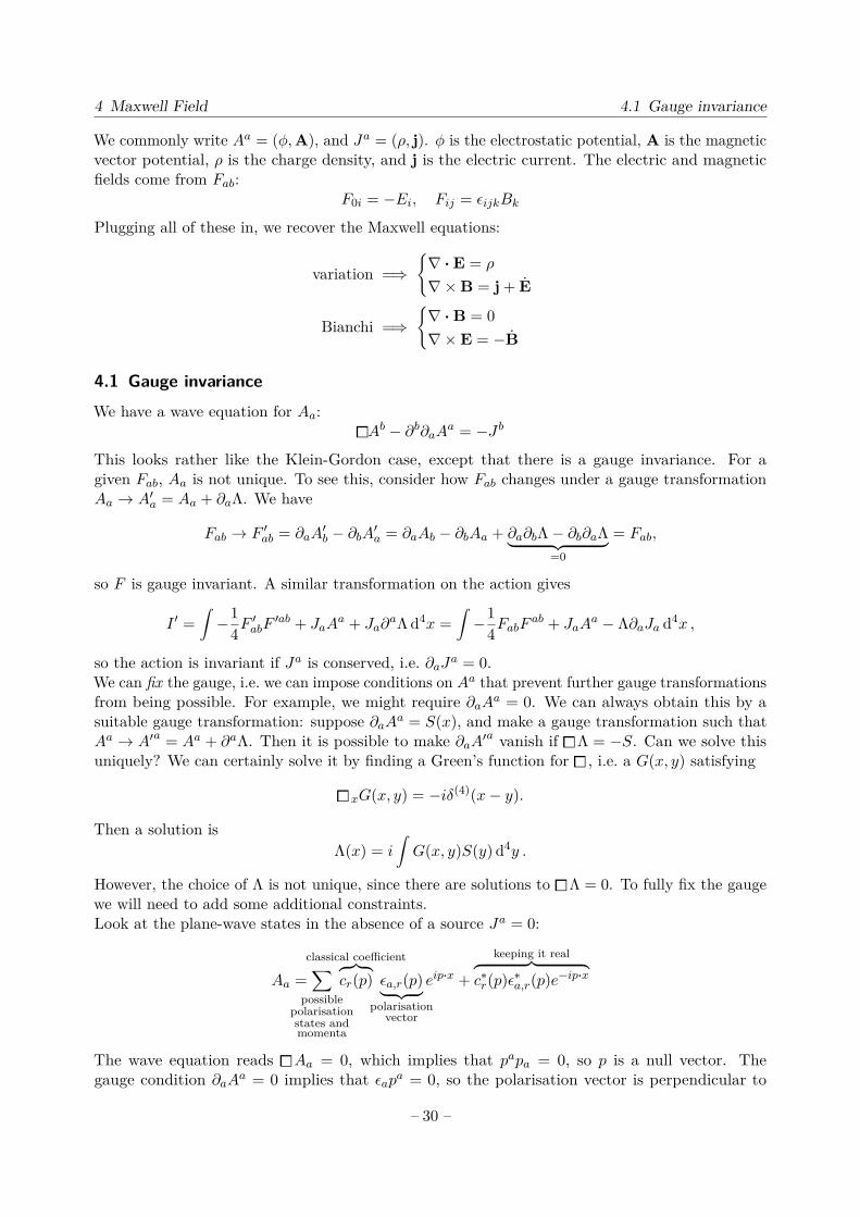
We commonly write Aa = (φ,A), and Ja = (ρ, j). φ is the electrostatic potential, A is the magneticvector potential, ρ is the charge density, and j is the electric current. The electric and magneticfields come from Fab:

F0i = −Ei, Fij = εijkBk

Plugging all of these in, we recover the Maxwell equations:

variation =⇒∇ ·E = ρ

∇×B = j + E

Bianchi =⇒∇ ·B = 0∇×E = −B

4.1 Gauge invarianceWe have a wave equation for Aa:

Ab − ∂b∂aAa = −Jb

This looks rather like the Klein-Gordon case, except that there is a gauge invariance. For agiven Fab, Aa is not unique. To see this, consider how Fab changes under a gauge transformationAa → A′a = Aa + ∂aΛ. We have

Fab → F ′ab = ∂aA′b − ∂bA′a = ∂aAb − ∂bAa + ∂a∂bΛ− ∂b∂aΛ︸︷︷︸

=0

= Fab,

so F is gauge invariant. A similar transformation on the action gives

I ′ =∫−1

4F′abF

′ab + JaAa + Ja∂

aΛ d4x =∫−1

4FabFab + JaA

a − Λ∂aJa d4x ,

so the action is invariant if Ja is conserved, i.e. ∂aJa = 0.We can fix the gauge, i.e. we can impose conditions on Aa that prevent further gauge transformationsfrom being possible. For example, we might require ∂aAa = 0. We can always obtain this by asuitable gauge transformation: suppose ∂aAa = S(x), and make a gauge transformation such thatAa → A′a = Aa + ∂aΛ. Then it is possible to make ∂aA′a vanish if Λ = −S. Can we solve thisuniquely? We can certainly solve it by finding a Green’s function for , i.e. a G(x, y) satisfying

xG(x, y) = −iδ(4)(x− y).

Then a solution isΛ(x) = i

∫G(x, y)S(y) d4y .

However, the choice of Λ is not unique, since there are solutions to Λ = 0. To fully fix the gaugewe will need to add some additional constraints.Look at the plane-wave states in the absence of a source Ja = 0:

Aa =∑

possiblepolarisationstates andmomenta

classical coefficient︷︸︸︷cr(p) εa,r(p)︸︷︷︸

polarisationvector

eip·x +

keeping it real︷︸︸︷c∗r(p)ε∗a,r(p)e−ip·x

The wave equation reads Aa = 0, which implies that papa = 0, so p is a null vector. Thegauge condition ∂aA

a = 0 implies that εapa = 0, so the polarisation vector is perpendicular to

– 30 –

4 Maxwell Field 4.2 Quantisation

the momentum. Consider now a gauge transformation Aa → A′a = Aa + ∂aΛ, and suppose thatΛ = f(p)eip·x is a plane wave. Then we have ∂aΛ = ipaf(p)eip·x, so

A′a = Aa + ipaf(p)eip·x ∼ cεaeip·x + ipaf(p)eip·x ∼ c′ε′aeip·x.

By an appropriate choice of f(p), one can make any single component of the polarisation vectorzero. Thus we can enforce the gauge condition A0 = 0, and this uses up all of the gauge degrees offreedom.The gauge choice A0 = 0 and ∂aA

a = 0 is known as the Coulomb gauge. In this gauge we canchoose the polarisation vector to have ε0 = 0, i.e. to be entirely spatial, ψa = (0, ε). We choose anormalisation of ε such that εaεa = εiε

i = 1.To see clearly the significance of ε, choose pa to represent a plane wave in the positive z-direction,so pa = (pz, 0, 0, pz), where pz > 0. Since εapa = ε · p = 0, a plane polarisation basis is

ε(x) a = (0, 1, 0, 0), ε(y) a = (0, 0, 1, 0).

The electric field E = −∇φ− A is parallel to A, so in the coulomb gauge, the polarisation vectoris parallel to the electric field.A sometimes more useful basis for the polarisation vectors is that of circular polarisation:

ε(+) a = 1√2

(0, 1,−i, 0), ε(−) a = 1√2

(0, 1, i, 0)

The sign ± corresponds to the electric field rotating anticlockwiseclockwise to the direction of travel of the

wave. This basis has some nice properties. In addition to the momenta being perpendicular to thepolarisation, we now also have orthogonality

ε∗r(p) · εr′(p) = δrr′ ,

and completeness ∑r

ε∗r,i(p)εr,j(p) = δij − δi3δj3.

In a more 3D covariant way (so for more p than just those in the positive z-direction), thecompleteness property takes the form∑

r

ε∗r,i(p)εr,j(p) = δij −pipj|p|2 .

4.2 QuantisationAs usual, to quantise we first start from the action. Decomposing things into space and time, wehave

I =∫

d3x dt− 12 F0iF

0i︸︷︷︸only place where there are time derivatives

−14FijF

ij

=∫

d3x dt = 12(∂0Ai − ∂iA0)(∂0Ai − ∂iA0)− 1

4FijFij .

There is no term involving A0 (this kind of thing always happens in theores with gauge invariance).The momentum conjugate to Ai is

πi = Ai − ∂iA0,

– 31 –


which is the electric field negated. The Hamiltonian is

H =∫

d3xπiAi − L

=∫

d3xπi(πi + ∂iA0)− 12E

2 + 12B

2

=∫

d3x12E

2 − Ei∂iA0 + 12B

2

=∫

d3x12E

2 +A0(∂iEi) + 12B

2.

We want to pick a gauge such that A0 = 0, so this must be true for all times. To make this work,one must choose ∂iEi = 0 — this is Gauss’ law.Now as before we expand A in a plane wave basis, with the classical coefficients promoted tooperators ar(p):

A =∑r

∫ d3p

(2π)31

2Ep

(ar(p)ε∗r(p)eip·x + a†r(p)εr(p)e−ip·x

)The corresponding momentum operator is

π =∑r

∫ d3p

(2π)31

2Ep

(i(−Ep)ar(p)ε∗r(p)eip·x + i(Ep)a†r(p)εr(p)e−ip·x

)= −i

∑r

∫ d3p

(2π)312(ar(p)ε∗r(p)eip·x − a†r(p)εr(p)e−ip·x

).

Now we can compute the equal time commutators. This looks straightforward, but ∂iEi = ∂iπi = 0

causes trouble. We could try to set

[Ai(x, t), πj(x′, t)] = iδijδ(3)(x− x′),

but this would be wrong, since acting with ∂(x) i gives zero on the left hand side, but a non-zeroquantity on the right hand side. Instead we define Pij = δij − ∂i∂j

∂2 , and set

[Ai(x, t), πj(x′, t)] = iPijδ(3)(x− x′).

Acting with partial derivatives now gives consistent results.It is worth clarifying what is meant by 1

∂2 . We want ∂2φ = f ⇐⇒ φ = 1∂2φ. There are two ways

we can ensure this. The first is to use the Green’s function defined by ∂2G(x, x′) = ∂(3)(x− x′).Then φ =

∫dy G(x, y)f(y) satisfies ∂2φ = f . The second way is to use Fourier transforms. Under

a Fourier transform we have ∂2φ→ −k2φ(k), so we can say 1∂2φ→ − 1

k2φ; this definition is thenequivalent to the first.Pij is a projection operator:

PijPjk =(δij −

∂i∂j∂2

)(δjk −

∂j∂k∂2

)= δik − 2∂i∂j

∂2 + ∂i∂j∂j∂k∂2∂2

= δik −∂i∂j∂2 = Pik.

The effect of Pij is thus to project out the unphysical part of the phase space.

– 32 –


We will use the notation f↔∂g = f∂g − (∂f)g. It can be shown that the a operators take the form

ar(p) = iεr(p) ·∫

d3x e−ip·x↔∂0A(x),

a†r(p) = −iε∗r(p) ·∫

d3x eip·x↔∂0A(x).

This can then be used to find the commutation rules for a, a†:

[ar(p), a†r′(q)] = (2π)32Epδrr′δ(4)(p− q)

[ar(p), ar′(q)] = [a†r(p), a†r′(q)] = 0

Thus a and a† can be interpreted as the creation and annihilation operators for particles ofmomentum p and polarisation r (like the Klein-Gordon field). We define the vacuum state |0〉 byar′(p) |0〉 = 0 for all r and p.We can find the normal ordered Hamiltonian to be

:H: =∑r

∫ d3p

(2π)31

2EpEpa

†r(p)ar(p).

The expectation value of this gives the energy of a given state, so we can interpret the particles asquanta of the electromagnetic field, i.e. photons.The propagator

∆ij = 〈0|TAi(x, t)Aj(y, t′)|0〉

is the amplitude for creation of a particle at y, t′ and annihilation at x, t (or vice versa, when timeordered). Let’s look at the t > t′ case. We have

∆ij =∑r,r′

∫ d3p

(2π)3d3p

(2π)31

4EpEq〈0|ε∗i,r(p)ar(p)eip·x εj,r′(q)a

†r′(q)e

−iq·y|0〉

=∑r,r′

∫ d3p

(2π)3d3p

(2π)31

4EpEqei(p·x−q·y)ε∗i,r(p)εj,r′(q) (2π)32Epδ(p− q)δrr′︸︷︷︸

from commutator

=∫ d3p

(2π)31

2Epeip·(x−y)∑

r

ε∗i,r(p)εj,r(p)︸︷︷︸=δij−

pipj

p2

,

so for x0 > y0 one finds exactly the Klein-Gordon field, apart from a factor of δij − pipjp2 . As before,

we can rewrite the propagator as a 4D integral:

∆ij = i

∫ d4p

(2π4)eip·(x−y) 1

p2 − iε

(δij −

pipjp2 − iε

)Acting on this with the d’Alembertian operator, we obtain

∆ij = i

∫ d4p

(2π)4 eip·(x−y) −p2

p2 − iε

(δij −

pipjp2 − iε

)= −i

∫ d4p

(2π)4 eip·(x−y)

(δij −

pipjp2 − iε

)

– 33 –

5 Path Integrals and Interaction 5 Path Integrals and Interaction

(this is just a Fourier transform under which pi → −i∂i)

= −i(δij −

∂i∂j∂2

)δ(4)(x− y),

so ∆ij is a Green’s function, but projected onto the subspace of objects annihilated by ∂i∂j .Now suppose we reintroduce a source term, so that we wish to solve Ai = Ji, δiJi = 0. Then wehave

Ai(x) =∫

d4y i∆ij(x− y)Jj(y),

and this automatically satisfies ∂iAi = 0.Return briefly to the Dirac action

I =∫

d4xψ(−iγ · ∂ +m)ψ.

For a particle in an electromagnetic field Aa, one can replace ∂a → ∂a− iqAa, where q is the chargeon the field (or particle). The action then becomes

I =∫

d4xψ(−iγ · (∂ − iqAa) +m)ψ.

This involves terms like ψψA.

5 Path Integrals and Interaction5.1 Quantum mechanicsConsider a particle of mass m moving in a potential V (x) in one space dimension. The Hamiltonianis H = p2

2m + V (x). Suppose the particle starts at position xi and time ti. We can calculate theamplitude to be at xf and tf as

〈xf , tf |xi, ti〉 = 〈xf |e−iHT |xi〉 in the Schrodinger picture,

where T = tf − ti. We can divide T into N steps, let ∆t = T/N , and take the limit as N →∞:

〈xf |e−iHT |xi〉 =∫ ∏

dx 〈xf |e−iH∆t|xN−1〉 . . . 〈x2|e−iH∆t|x1〉〈x1|e−iH∆t|xi〉

This works because |x〉 form a complete set, so∫

dx |x〉〈x| = 1. This integral just requires evaluationof 〈x′|e−iH∆t|x〉.In quantum mechanics we have position eigenstates |x〉 and momentum eigenstates |p〉, and theirscalar products are 〈p|x〉 = 1√

2πeipx. Thus we have

⟨x′∣∣e−iH∆t∣∣x⟩ =

⟨x′∣∣ei∆t

[p22m+V (x)

]∣∣x⟩=∫

dp⟨x′∣∣ei∆t

[p22m+V (x)

]∣∣p⟩ 〈p|x〉(O(∆t2) terms are negligible in the limit ∆t→ 0)

=∫

dp e−∆tV (x′)e−i∆tp2/2m ⟨x′∣∣p⟩ 〈p|x〉

=∫

dp e−∆tV (x′)e−i∆tp2/2m 1

2πeip(x′−x).

– 34 –

5 Path Integrals and Interaction 5.1 Quantum mechanics

In the limit as N →∞,∆t→ 0, we have x′ − x ≈ x∆t. Thus we have

〈xf , tf |xi, ti〉 =∫ ∏

i

dxi∏j

dpj e−i∆tp2j/2m−i∆tV (xi) 1

2πeipj xi∆t

(now exchange∏e... for e

∑...)

=∫ ∏

i

dxi dpi2π e−i

∑(p2i /2m+V (xi)−pxi)∆t.

In the limit that N →∞, the sum over integrals becomes its own kind of integral. We use D[x, p]to mean integrate over all x and all p at each instant of time. Then we have

〈xf |e−iHT |xi〉 =∫

D[x, p] e−i∫

dt(p2/2m+V−px)

=∫

D[x, p] e−i∫

dt(H−px).

This is a phase space path integral. We integrate over all of phase space at each instant of time. Itis possible to integrate out the momenta from this expression; at each moment in time, one gets∫ dp

2πe−ip2/2m+ipx =

∫ ∞−∞

dp2πe

− i2m (p−xm)2

eimx2/2

= (phase) 12π√π · 2meimx2/2.

Thus we have

〈xf , tf |xi, ti〉 = (phase)∫

Dx(m

2π

)N/2ei∫

dt(mx2

2 −V)

(up to normalisation)

=∫

Dx ei∫

dt(mx2

2 −V)

=∫

Dx ei∫

dtL,

where L is the Lagrangian. The exponent is just the action multiplied by i, so we have

〈xf , tf |xi, ti〉 = N

∫Dx eiS .

This is a coordinate space path integral. It is an integral over all possible paths, weighted byeiS . Note that the paths can be non-smooth and even non-continuous, because each x-integral isindependent of all others. Quantum mechanically, we interpret this as the particle exploring allpossible parts of space.One might protest about the apparently infinite normalisation factor. The resolution of thisdifficulty is to calculate normalisation some other way, for example using

1 =∫〈xi, ti|xf , tf 〉〈xf , tf |xi, ti〉 dxf .

This is easy to calculate for a free particle (in which case there is no normalisation possible), andfor a simple harmonic oscillator.

– 35 –

5 Path Integrals and Interaction 5.2 Fields

5.2 FieldsWe now extrapolate the above to field theory. A real free scalar field φ has Lagrangian

L = −12(∂φ)2 − 1

2m2φ2.

We can view φ as being dependent on all points in spacetime. Then the path integral for the scalarfield is given by ∫

D[φ] ei∫Ld4x.

The integral is taken over all spacetime points, and is weighted by eiS , where S =∫L d4x is the

action for the field theory.Consider now adding a source to our theory, so that the action takes the form

I =∫

d4x−12(∂φ)2 − 1

2m2φ2︸︷︷︸

free scalar field

+ iJφ︸︷︷︸source term

=∫

d4x12φ( −m2)φ+ iJφ.

The equations of motion are nowLφ = iJ(x),

where L = − +m2 is the Klein-Gordon operator. We use L−1 as a shorthand for the Green’sfunction expression of the operator L:

φ(x) = iL−1J = i

∫G(x, x′)J(x′) d4x where LG = δ(4)(x− x′)

We define the following path integral, where the 0 subscript indicates that we are working with afree field:

Z0(J) =∫

Dφ ei∫Ld4x

=∫

Dφ ei∫− 1

2φLφ+iJφd4x

=∫ ∏

x

dφ(x)∏x

e−i2φLφ−Jφ

(this integral can be done since it is a Gaussian integral)

=∫ ∏

x

dφ(x)∏x

e−i2 (φ−iJL−1)L(φ−iL−1J)e−

i2JL

−1J

(define φ = φ− iJL−1)

=∫

Dφ exp(i

∫d4x− 1

2 φLφ−12JL

−1J

)Note that since JL−1 is independent of φ, we have Dφ = Dφ. Thus we can write

Z0(J) = Z0(0) exp(− i2

∫d4xJL−1J

)= Z0(0) exp

(− i2

∫d4x d4x′ J(x)G(x, x′)J(x′)

).

– 36 –

5 Path Integrals and Interaction 5.2 Fields

Now look at the functional derivatives of Z0(J) with regard to J . We haveδZ0(J)δJ(w) = Z0(0) exp

(− i2

∫d4x d4x′ J(x)G(x, x′)J(x′)

)(− i

2

∫d4x′′ d4x′′′G(x′′, x′′′)J(x′′′)δ(x′′ − w)

− i

2

∫d4x′′ d4x′′′ J(x′′)G(x′′, x′′′)δ(x′′′ − w)

)= Z0(0) exp(. . .)

(−i∫

d4x d4x′G(x, x′)δ(x− w)J(x′))

= Z0(0) exp(. . .)(−i∫

d4x′G(w, x′)J(x′)).

Also,δ2Z0(J)

δJ(w)δJ(z) = Z0(0) exp(. . .)(−∫

d4x′′G(z, x′′)J(x′′)∫

d4x′G(w, x′)J(x′)− i∫

d4x′G(w, x′)δ(x′ − z))

= Z0(0) exp(. . .)(−∫

d4x′′G(z, x′′)J(x′′)∫

d4x′G(w, x′)J(x′)− iG(w, z)).

Now put J = 0. We obtain

1Z0(0)

δ2Z0(J)δJ(w)δJ(z)

∣∣∣∣∣J=0

= −iG(w, z) = ∆F (w − z) = 〈0|Tφ(w)φ(z)|0〉 .

It is an exercise to show that1

Z0(0)δ4Z0(J)

δJ(w)δJ(z)δJ(s)δJ(t)

∣∣∣∣∣J=0

= ∆F (w−z)∆F (s−t)+∆F (z−t)∆F (w−s)+∆F (w−t)∆F (z−s).

In general, we have1

Z0(0)δ(odd)Z0(J)

δJ(z1) . . . δJ(zn)

∣∣∣∣∣J=0

= 0.

The even case is known as Wick’s theorem:1

Z0(0)δ(even)Z0(J)

δJ(z1) . . . δJ(zn)

∣∣∣∣∣J=0

=∑all

possiblepairings

∆F (zk1 − zk2)∆F (zk3 − zk4) . . .︸︷︷︸n2 terms

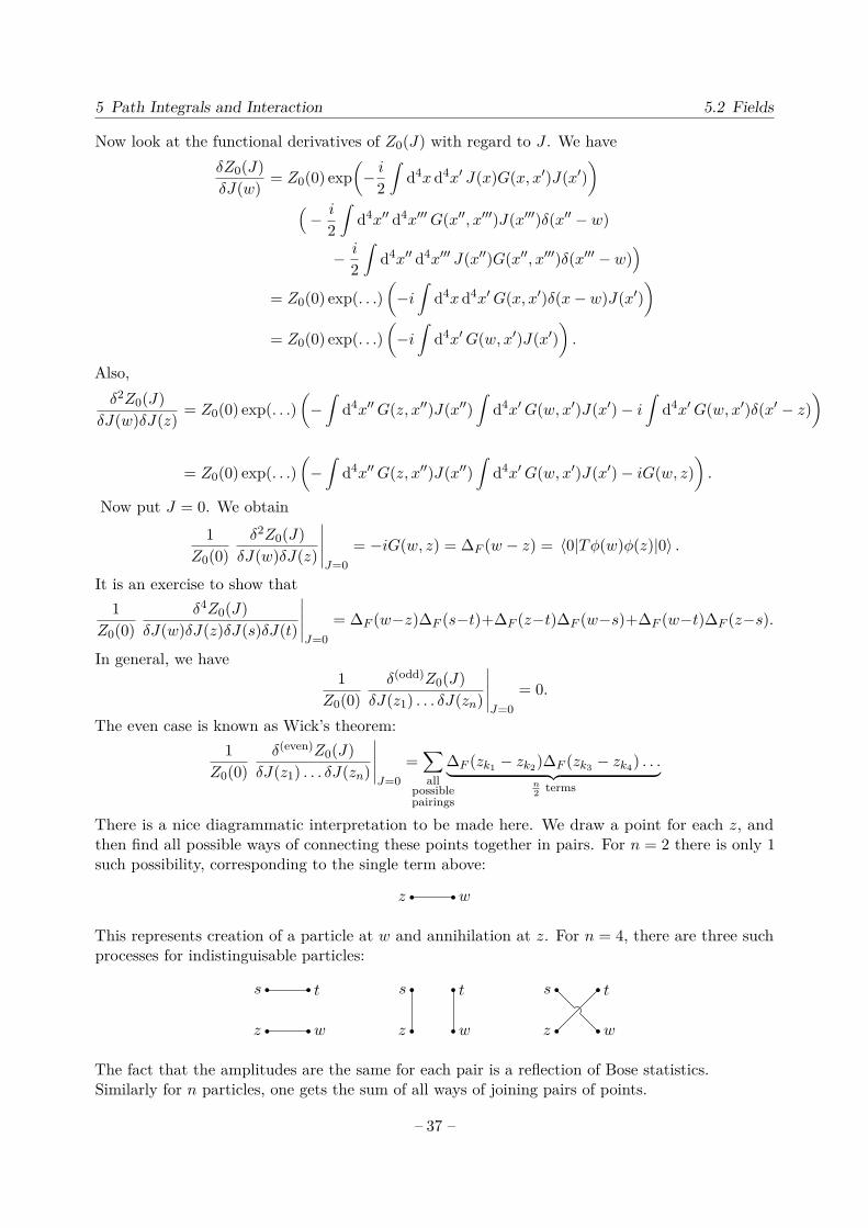
There is a nice diagrammatic interpretation to be made here. We draw a point for each z, andthen find all possible ways of connecting these points together in pairs. For n = 2 there is only 1such possibility, corresponding to the single term above:

z w

This represents creation of a particle at w and annihilation at z. For n = 4, there are three suchprocesses for indistinguisable particles:

z w

s t

z w

s t

z w

s t

The fact that the amplitudes are the same for each pair is a reflection of Bose statistics.Similarly for n particles, one gets the sum of all ways of joining pairs of points.

– 37 –

5 Path Integrals and Interaction 5.3 Interaction

5.3 InteractionThe only allowed interaction terms (for reasons) are of the form LI = −λφ4

4! or +gφ3

3! . The fullLagrangian is

L = −12(∂φ)2 − 1

2m2φ2 + LI + iJφ.

The resultant equations of motion (setting J = 0) are

( −m2)φ = gφ2

2 or − λφ3

6 .

These are non-linear equations for which general analytic solutions do not exist. Even if we couldsolve these equations, the solutions could not be linearly superposed. Therefore we will treat thesecases with perturbation theory, expanding in powers of g or λ.We have

Z1(J) =∫

Dφ ei∫L0+LId4x =

∫Dφ ei

∫LId4xei

∫L0d4x.

Note that − δδJ(x) acting on ei

∫L0 d4x gives φ(x)ei

∫L0 d4x. Hence we can replace ei

∫LI [φ(x)] d4x

by ei∫LI(− δδJ(x)

)d4x in the above expression. We obtain

Z1(J) =∫

Dφ ei∫LI(− δδJ(x)

)d4xei∫L0d4x = e

i∫LI(− δδJ(x)

)d4xZ0(J).

Thus we have (up to normalisation)

Z1(J) ∼ exp(i

∫LI(− δ

δJ(x)

))exp

(12

∫d4x d4y J(x)∆F (x− y)J(y)

)︸︷︷︸

∼Z0

. (∗)

5.4 φ3 theory

Let’s set LI = gφ3

3! and evaluate (∗). We have

Z1(J) =∞∑V=0

[∫d4x

(− δ

δJ(x)

)3]V gV iV

V !(3!)V ×∞∑P=0

[∫d4y d4z J(y)∆F (y − z)J(z)

]P 1P !

12P .

Note that this is an asymptotic series, but not a convergent one. Each term in the series will be∼ gV JE∆P

F , where E = 2P − 3V . We organise the expansion in powers of E and V .The diagrammatic analogy continues here. We will start with the diagrams, and then explain howthey relate to the series expansion for Z1(J). For each E, V, P , we draw all possible graphs with Vvertices, P internal lines, and E external lines. Internal vertices must be trivalent.At E = 0, V = 2, P = 3 we have:

E = 0, V = 4, P = 6:

– 38 –

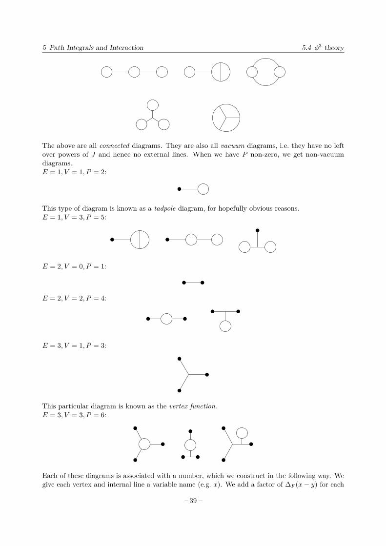
5 Path Integrals and Interaction 5.4 φ3 theory

The above are all connected diagrams. They are also all vacuum diagrams, i.e. they have no leftover powers of J and hence no external lines. When we have P non-zero, we get non-vacuumdiagrams.E = 1, V = 1, P = 2:

This type of diagram is known as a tadpole diagram, for hopefully obvious reasons.E = 1, V = 3, P = 5:

E = 2, V = 0, P = 1:

E = 2, V = 2, P = 4:

E = 3, V = 1, P = 3:

This particular diagram is known as the vertex function.E = 3, V = 3, P = 6:

Each of these diagrams is associated with a number, which we construct in the following way. Wegive each vertex and internal line a variable name (e.g. x). We add a factor of ∆F (x− y) for each

– 39 –


internal line, where x and y are the vertices it connects. We put in an integral∫

d4x g for eachvertex and

∫d4xJ(x) for each external line. We multiply by a phase factor iP−2V , and finally

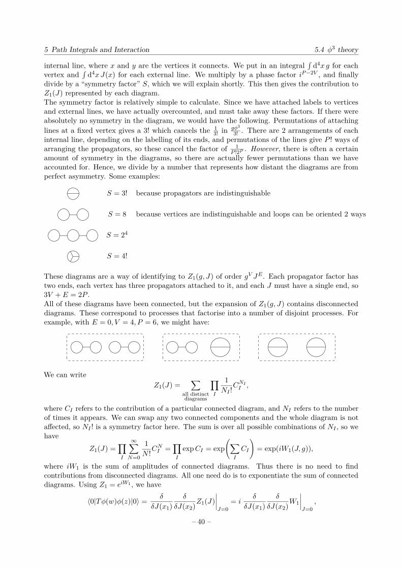
divide by a “symmetry factor” S, which we will explain shortly. This then gives the contribution toZ1(J) represented by each diagram.The symmetry factor is relatively simple to calculate. Since we have attached labels to verticesand external lines, we have actually overcounted, and must take away these factors. If there wereabsolutely no symmetry in the diagram, we would have the following. Permutations of attachinglines at a fixed vertex gives a 3! which cancels the 1

3! in gφ3

3! . There are 2 arrangements of eachinternal line, depending on the labelling of its ends, and permutations of the lines give P ! ways ofarranging the propagators, so these cancel the factor of 1

P !2P . However, there is often a certainamount of symmetry in the diagrams, so there are actually fewer permutations than we haveaccounted for. Hence, we divide by a number that represents how distant the diagrams are fromperfect asymmetry. Some examples:

S = 3! because propagators are indistinguishable

S = 8 because vertices are indistinguishable and loops can be oriented 2 ways

S = 24

S = 4!

These diagrams are a way of identifying to Z1(g, J) of order gV JE . Each propagator factor hastwo ends, each vertex has three propagators attached to it, and each J must have a single end, so3V + E = 2P .All of these diagrams have been connected, but the expansion of Z1(g, J) contains disconnecteddiagrams. These correspond to processes that factorise into a number of disjoint processes. Forexample, with E = 0, V = 4, P = 6, we might have:

We can writeZ1(J) =

∑all distinctdiagrams

∏I

1NI !

CNII ,

where CI refers to the contribution of a particular connected diagram, and NI refers to the numberof times it appears. We can swap any two connected components and the whole diagram is notaffected, so NI ! is a symmetry factor here. The sum is over all possible combinations of NI , so wehave

Z1(J) =∏I

∞∑N=0

1N !C

NI =

∏I

expCI = exp(∑

I

CI

)= exp(iW1(J, g)),

where iW1 is the sum of amplitudes of connected diagrams. Thus there is no need to findcontributions from disconnected diagrams. All one need do is to exponentiate the sum of connecteddiagrams. Using Z1 = eiW1 , we have

〈0|Tφ(w)φ(z)|0〉 = δ

δJ(x1)δ

δJ(x2)Z1(J)∣∣∣∣J=0

= iδ

δJ(x1)δ

δJ(x2)W1

∣∣∣∣J=0

,

– 40 –


and we can also calculate

〈0|Tφ(x1)φ(x2)φ(x3)φ(x4)|0〉 = [iδ1δ2δ3δ4W − δ1δ2Wδ3δ4W − δ1δ3Wδ2δ4W − δ1δ4Wδ2δ3W ] .

Consider now the amplitude for four particle interactions to order g2, with two particles in thepast and two particles in the future. If we label each external line (particle), then there are threepossible diagrams:

1

2

1′

2′

k1

k2

k′1

k′2k = k1 + k2

2 2′

1 1′

k2

k′2

k1

k′1

k = k1 − k′1

1

2′2

1′k1

k2

k′1

k′2

k = k1 − k′2

Rather than treat these amplitudes as functions of spacetime, we instead look at their Fouriertransforms and label the particle states by their momenta. To do this we must translate thecomputational rules into momentum space. In coordinate space one has to integrate over allposition in spacetime of each vertex. We have

〈f |i〉 = ig2∫ d4k

(2π)41

k2 +m2 − iε[(2π)4δ4(k1 + k2 − k)(2π)4δ4(k′1 + k′2 − k)

+ (2π)4δ4(k1 − k′1 − k)(2π)4δ4(k2 − k′2 − k)+ (2π)4δ4(k1 − k′2 − k)(2π)4δ4(k′1 − k2 − k)

]= ig2(2π)4 δ4(k1 + k2 − k′1 − k′2)︸︷︷︸

momentum conservation

T,

whereT = 1

(k1 + k2)2 +m2 − iε+ 1

(k1 − k′1)2 +m2 − iε+ 1

(k1 − k′2)2 +m2 − iεis the transfer matrix for this process. This is tree-level scattering (no loops).The rules for calculating these amplitudes with diagrams for a given theory are known as itsFeynman rules. To summarise, the momentum space Feynman rules are:

1. Draw all diagrams to the appropriate order.

2. Label each ingoing and outgoing line with its momentum.

– 41 –


3. Conserve momentum at each vertex, so add a factor (2π)4δ(4)(k1 + k2 + k3).

4. For each internal line, add a factor of the Feynman propagator −ik2+m2−iε .

5. For each vertex, add a factor of ig.

6. For each undetermined momentum, integrate∫ d4k

(2π)4 .

7. Divide by the symmetry factor.

8. Add all terms to get the transfer matrix.

5.5 φ4 theory

If we have LI = −λφ4

4! , then the Feynman rules are exactly the same, except vertices must now be4-valent, and come with a factor of −iλ. Let’s calculate the transfer matrix for the scattering fromtwo particles to two particles, to order λ2. We have the following diagrams:

k1

k′2k2

k′1 k1

k − k1 + k2

k′1

k2

k

k′2

We ignore other diagrams for now. Using the Feynman rules, this translates to

iT = λ+ −λ2

2

∫ d4k

(2π)4−i

k2 +m2 − iε−i

(k − l)2 +m2 − iε,

where l = k1 + k2. Set m2 = 0 (so a massless field), The O(λ2) part

f(s = l2) = iλ2

2

∫ d4k

(2π)41k2

1(k − l)2

is a divergent integral, so we will need to regularise it in some fashion.A commonly used identity for transforming integrals of this form is the so-called “Feynmanparameter formula”:

1xy

=∫ 1

0dα 1

(αx+ (1− α)y)2

Using this with x = (k − l)2 and y = k2, we have

f(s) = iλ2

2

∫ d4k

(2π)4

∫ 1

0dα 1

[α(k − l)2 + (1− α)k2]2

= iλ2

2

∫ d4k

(2π)4

∫ 1

0dα 1

[k2 − 2αk · l + αl2]2

= iλ2

2

∫ d4k

(2π)4

∫ 1

0dα 1

[(k − αl)2 + α(1− α)l2]2

– 42 –


(now shift the origin of the momentum integral)

= iλ2

2

∫ d4k

(2π)4

∫ 1

0dα 1

[k2 + α(1− α)l2]2 .

We will use Pauli-Villars regularisation: we introduce a cut-off for large momenta. Note that∫

d4k

is an integral over all momenta, with d4k = d3k dk0, and k2 = −k02 + k2. The (ignored here)factors of iε amount to saying that the integration over k0 is along the imaginary axis. Hence wecan rotate the k0 contour, setting k0 → ik0. Now we have k2 = k02 + k2. We get

f(s) = λ2

2

∫ d4k

(2π)4

∫ 1

0dα 1

[k2 + α(1− α)l2]2

where k is now in real space, and k2 is Euclidean. Introduce polar coordinates in momentum space,so that d4k → k3 dk dΩk, where dΩk is the volume element of the unit 3-sphere. Nothing dependson the direction of k, so

∫dΩk = 2π2. Hence we have

f(s) = λ2

16π2

∫ Λ

0k3 dk

∫ 1

0dα 1

[k2 + α(1− α)l2]2 .

We integrate only up to |k| = Λ — this is the momentum cut-off of the Pauli-Villars regularisation.We write A =

√α(1− α)l2. We have

f(s) = λ2

16π2

∫ Λ

0k3 dk

∫ 1

0dα 1

[k2 +A2]2

(now rescale k → z = k/A)

= λ2

16π2

∫ 1

0dα∫ Λ/A

0z3 dz 1

(z2 + 1)2

(set z = sinh θ)

= λ2

16π2

∫ 1

0dα∫ Λ/A

0

sinh3 θ cosh θ dθcosh4 θ

= λ2

16π2

∫ 1

0dα∫ Λ/A

0tanh3 θ dθ

= λ2

16π2

∫ 1

0dα[log cosh θ − 1

2 tanh2 θ

]z=Λ/A

0

= λ2

16π2

∫ 1

0dα[

12 log

(1 + z2

)− z2

2(1 + z2)

]Λ/A

0

= λ2

16π2

∫ 1

0dα[

12 log

(1 + Λ2

A2

)− Λ2/A2

2(1 + Λ2/A2)

]

= λ2

32π2

∫ 1

0dα[log(

Λ2

A2

)+ log

(1 + A2

Λ2

)− 1

1 +A2/Λ2

](now assume the cutoff is large, i.e. Λ2 A2)

≈ λ2

32π2

∫ 1

0dα[log(Λ2)− log

(l2α(1− α)

)− 1

]= λ2

32π2

[α log Λ2

l2− α logα+ (1− α) log(1− α)− 1− α

]1

0

= λ2

32π2 log Λ2

l2+ constant.

– 43 –

5 Path Integrals and Interaction 5.6 Higher loops

Observe that although the regularised amplitude is finite, we really want to take the limit as Λto∞,since we are supposed to integrate over all momenta.So the amplitude for 2 particles to go to 2 particles, for the case s = l2, is given by

iT (s) = λ+ λ2

32π2 log Λ2

s+ (constant).

The input into the theory is a coupling constant λ, and an incoming energy parametrised by s, butT depends on Λ, so this looks like it might be nonsense. To get around this, we write λR = T (s0):this is the renormalised coupling constant. In an actual experiment, we measure the amplitude atsome energy. Consider the amplitude T (s0) and compare it to T (s1). We have

T (s1)− T (s0) = λ2

32π2 log(s1s0

),

so the difference between the amplitudes is finite. We have

λR = λ+ λ2

32π2 log Λ2

s0.

Inverting this series, we obtain

λ ≈ λR −λ2R

32π2 log Λ2

s0.

Hence we can find

T (s1) = λ+ λ2

32π2 log Λ2

s1

= λR −λ2R

32π2 log Λ2

s0+ λ2

R

32π2 log Λ2

s1+O(λ3

R)

≈ λR −λ2R

32π2 log s1s0.

We choose λR to be finite. Since Λ→∞, this means we must have λ→∞. So the output is: givenamplitudes at some energy scale, you can calculate amplitudes at another energy scale.The justification of this method is that it (sometimes) works.There are only two other things that can be renormalised: the masses of particles, and the overallnormalisation of the fields (wavefunction renormalisation).The 1-loop diagrams that we did not consider above only add a constant for fixed external momentato the amplitudes, so they do not change differences in amplitudes.

5.6 Higher loopsThere are contributions to the amplitude with more loops:

+ + + + . . .

If we include powers of ~, then an L-loop diagram contributes a term to the amplitude of order ~L.Note that the amplitude as a power series expansion in powers of the coupling constant is usuallyasymptotic. If we write T =

∑λnTn, then this series becomes useless when n ∼ 1

λ .

– 44 –

5 Path Integrals and Interaction 5.7 Free fermions

Suppose we have a Feynman diagram with φN interactions that has P propagators, E externallines, V vertices, and L loops (i.e. the number of undetermined momenta in the diagram). Sinceeach propagator has 2 ends, we can write E + 2P = NV . Also, the momenta are constrained byconservation at each vertex and for the overall diagram, so the number of undetermined momentais L = P − V + 1. If we were to evaluate the Feynman diagram, with a momentum cutoff Λ, wewould get something that looked like

(momentum)4L︸︷︷︸d4p

for loops

1(momentum)2P︸︷︷︸

propagators

∼ Λ4L−2P .

We call this exponent D = 4L − 2P the primitive degree of divergence (if D ≥ 0). We haveD = 4(P − V + 1) − 2P = 2P − 4V − 4. For D = 0, as Λ → ∞ we encounter a logarithmicdivergence log Λ2, as in the previous section. For higher D we get faster divergences. For exampleD = 2 leads to a quadratic divergence. If D < 0, then the contribution to the amplitude vanishesas Λ→∞.In a general diagram, D = 2P − 4V + 4 = NV − 4V + 4−E = V (N − 4) + 4−E. So from this wecan more or less see that arbitrary interactions are impossible. For N ≤ 4, there are only a finitenumber of different types of divergence: we say this theory is renormalisable. For N ≥ 5, there arean infinite number of types of divergence. Such a theory is nonrenormalisable, and do not exist asQFTs.

5.7 Free fermionsIf we add a source term to the Dirac action, we have

S =∫

d4xψ(iγa∂a −m)ψ + ηψ + ψη,

where η is a spinor.ψ and ψ are anticommuting objects. We have

ψ ∼ beip·x + d†e−ip·x,

where b and d are anticommuting objects, so br(p), bs(q) = 0 and so on.In the path integral for the scalar field, we treated φ and J as functions which reproduced whatcame from the operators. We do the same here, treating ψ and ψ as anticommuting functions. Theyare Grassman variables, anticommuting with each other, but commuting with ordinary numbers.A set of anticommuting objects ψi, i = 1, . . . , N obey

ψi, ψj = ψiψj + ψjψi = 0.

ψi could be the value of a field at some point in spacetime, in which case this is an infinite set, orthis could just be a finite collection of variables.The partition function for the Dirac action reads

Z0(η, η) =∫

DψDψ ei∫

d4xψ(iγ·∂−m)ψ+ηψ+ψη.

If we recall that ψ is the generalised coordinate and ψ is the generalised momentum, we see thatthis is an integral over all phase space. The exponent in the integral is the same as H − p · q (thisholds for theories with only one time derivative).

– 45 –


Consider a situation where N = 1, with one anticommuting object ψ. Since ψ2 = 0, any functionof ψ can be written

f(ψ) = a+ bψ.

If f is commuting, then a is a complex number, and b is anticommuting, and we also have f = a−ψb.If f is anticommuting, then a is anticommuting, and b is a complex number.Anticommuting and commuting functions form a graded algebra. For a given f we define

εf =

0 commuting1 anticommuting

.

(We sometimes call an object with εf = 0 Grassman even, and an object with εf = 0 Grassmanodd.) Then we use a graded commutator

[f, g]± = fg ± (−)εf εggf = 0.

Note that the ordering of variables is important when doing things such as derivatives. Supposef(ψ) = a+ bψ is even. We define ∂

∂ψ to act on the right on whatever it finds, so we have

∂f

∂ψ= ∂

∂ψ(a+ bψ) = ∂

∂ψ(−ψb) = −b.

Integration of these functions is defined by analogy with integrating a real variable from −∞ to ∞.Take any (even) function of a real variable f(x). Then as long as f(x) is appropriately bounded(so that

∫∞−∞ f(x) dx exists), then integration has two notable properties. These are linearity∫ ∞

−∞Cf(x) dx = C

∫ ∞−∞

f(x) dx

and translation symmetry ∫ ∞−∞

f(x+ y) dx =∫ ∞−∞

f(x) dx .

In order to replicate these properties for integration of Grassman variables, we must set (up to aconstant multiple): ∫

dψ 1 = 0 and∫

dψ ψ = 1.

We have chosen this normalisation so that integration for odd quantities is the same as differentiationon the left.Now consider N > 1 and suppose we have a collection of odd variables ψi, i = 1, . . . , N , obeting[ψi, ψj ]+ = δij . Any function of these variables can be Taylor expanded as

f(ψ) = a+ biψi + 12cijψiψj + 1

6dijkψiψjψk + · · ·+ d1N !εij...Nψ1 . . . ψN .

Each coefficient in this expansion is completely antisymmetric. Note that Taylor expansions of ψalways stop for finite N .Integration follows as above. Now we have

∫dψi ψj = δij . Note that in the following integral, the

only term that survives is the last one:∫dψN dψN1 . . . dψ2 dψ1︸︷︷︸

dNψ

f(ψ) = d

– 46 –


Under a change of variables ψi = Jijψ′j , we have

f(ψ) = a = biJijψ′j + · · ·+ d

N ! Jii′Jjj′ . . . JNN ′εij...N︸︷︷︸

=det(J)εi′j′...N′

ψi′ . . . ψN ′ ,

and so the integral changes in the following way:∫dNψ f(ψ) = (detJ)−1

∫dNψ′ f(ψ)

Note that the Jacobian factor in the change of variables comes with exponent −1 for Grassmanodd variables, rather than +1 for ordinary commuting variables.We are now ready to calculate the free Dirac path integral. Write D = iγ · ∂ − m, the Diracoperator. We have

Z0(η, η) =∫

DψDψ ei∫

d4x(ψDψ+ψη+ηψ)

=∫

DψDψ ei∫

d4x((ψ+ηD−1)D(ψ+D−1η)−ηD−1η)

(now change variables ψ → ψ −D−1η = ψ′, and note det J = 1)

=∫

Dψ′Dψ′ exp(i

∫d4xψ

′Dψ′

)︸︷︷︸

independent of η

exp(−i∫

d4x ηD−1η

).

Therefore we can write

Z0(η, η) = N exp(−i∫

d4x d4y η(x)D−1(x, y)η(y)),

where N is some normalisation factor, and D−1(x, y) is a Green’s function for the Dirac operator.Note that (treating η and η as independent) we have

δ

δη(y)

∫d4x η(x)ψ(x) + ψ(x)η(x) =

∫d4x δ(x− y)ψ(x) = ψ(y)

andδ

δη(y)

∫d4x η(x)ψ(x) + ψ(x)η(x) =

∫d4x− ψ(x)δ(x− y) = −ψ(y).

Hence we have

〈0|Tψα(x)ψβ(y)|0〉 = 1i

δ

δη(x) iδ

δη(y)Z0(η, η)∣∣∣∣η,η=0

= iSF (x, y),

where SF is the propagator for the Dirac field.If we split the Lagrangian into (free terms) + (interactions), we get an interaction Lagrangian whichlooks like

Z1 ∼∫

DψDψ . . . ei∫L0+LI(ψ,ψ)d4x

∼ exp(iLI

(iδ

δη,−i δ

δη

))Z0(η, η).

Following this through, we can reproduce the perturbation series for theories with fermions. Wecan follow the same procedure as for bozons to fully develop a set of Feynam rules for fermions.

– 47 –

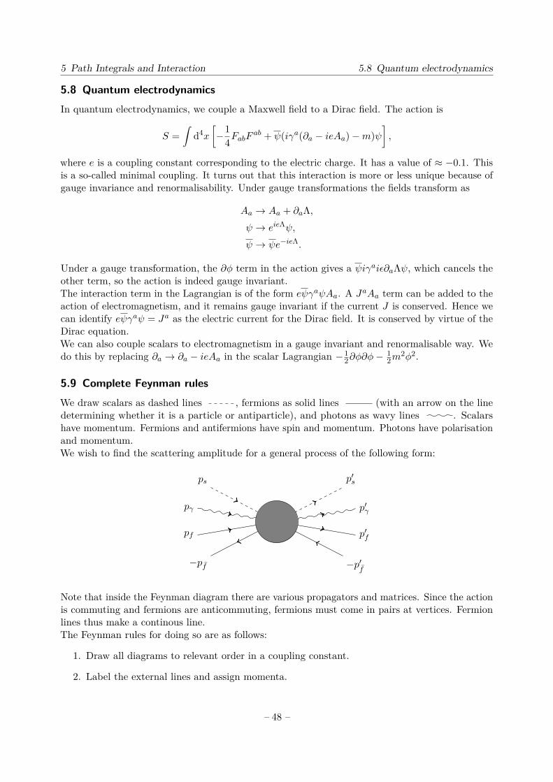
5 Path Integrals and Interaction 5.8 Quantum electrodynamics

5.8 Quantum electrodynamicsIn quantum electrodynamics, we couple a Maxwell field to a Dirac field. The action is

S =∫

d4x

[−1

4FabFab + ψ(iγa(∂a − ieAa)−m)ψ

],

where e is a coupling constant corresponding to the electric charge. It has a value of ≈ −0.1. Thisis a so-called minimal coupling. It turns out that this interaction is more or less unique because ofgauge invariance and renormalisability. Under gauge transformations the fields transform as

Aa → Aa + ∂aΛ,ψ → eieΛψ,

ψ → ψe−ieΛ.

Under a gauge transformation, the ∂φ term in the action gives a ψiγaiε∂aΛψ, which cancels theother term, so the action is indeed gauge invariant.The interaction term in the Lagrangian is of the form eψγaψAa. A JaAa term can be added to theaction of electromagnetism, and it remains gauge invariant if the current J is conserved. Hence wecan identify eψγaψ = Ja as the electric current for the Dirac field. It is conserved by virtue of theDirac equation.We can also couple scalars to electromagnetism in a gauge invariant and renormalisable way. Wedo this by replacing ∂a → ∂a − ieAa in the scalar Lagrangian −1

2∂φ∂φ−12m

2φ2.

5.9 Complete Feynman rulesWe draw scalars as dashed lines , fermions as solid lines (with an arrow on the linedetermining whether it is a particle or antiparticle), and photons as wavy lines . Scalarshave momentum. Fermions and antifermions have spin and momentum. Photons have polarisationand momentum.We wish to find the scattering amplitude for a general process of the following form:

ps p′s

pγ p′γ

pf p′f

−pf −p′f

Note that inside the Feynman diagram there are various propagators and matrices. Since the actionis commuting and fermions are anticommuting, fermions must come in pairs at vertices. Fermionlines thus make a continous line.The Feynman rules for doing so are as follows:

1. Draw all diagrams to relevant order in a coupling constant.

2. Label the external lines and assign momenta.

– 48 –

5 Path Integrals and Interaction 5.9 Complete Feynman rules

3. Label each internal line with the appropriate wavefunction:

Field Incoming Outgoing

Fermion us(pf ) us(p′f )Antifermion vs(pf ) vs(p′f )Scalar 1 1Photon ε∗λ(pγ) εγ(p′γ)

4. Add a propagator for each internal line:

Field Propagator

Fermion −i(−/k +m)k2 +m2 − iε

Scalar −ik2 +m2 − iε

Photon −iηab

k2 − iε

5. Determine the symmetry factor and divide by it.

6. Integrate over all undetermined momenta with ±∫ d4k

(2π)4 , where + is for scalars and photons,and − is for fermions.

7. Add all diagrams to give the total amplitude but in a way that is antisymmetric over anyoutgoing fermions.

As an example consider electron positron annihilation e+e− → γγ to order e2. We have thefollowing diagrams:

e−

e+

γ

γ

−p2, s2

p1, s1

k′2, λ2

k′1, λ1

p1 − k′1

e−

e+

γ

γ

−p2, s2

p1, s1

k′1, λ1

k′2, λ2

p1 − k′2

Mandelstam variables are often used to find how these diagrams deal with momenta. The Mandel-stam variables are

s = −(p1 + p2)2 (measure of left to right momentum),t = −(p1 − k′1)2 (measure of momentum transfer in first diagram),u = −(p1 − k′2)2 (measure of momentum transfer in second diagram).

Note that since s+ t+u = 2m2, where m2 is the sum of the masses squared for all external particles,two of these variables fully determine the third.Using the above Feynman rules we can then determine the transfer matrix (i.e. the amplitudemodulo momentum conservation):

T = e2εaλ1(k′1)εbλ2(k′2)vs2(p2)[γb

−(/p1 − /k′1) +m

(p1 − k′1)2 +m2 − iεγa + γa

−(/p1 − /k′2) +m

(p1 − k′2)2 +m2 − iεγb

]us1(p1)

– 49 –

5 Path Integrals and Interaction 5.9 Complete Feynman rules

**Non-examinable** In terms of Mandelstam variables, we have

14∑spins

∑λ1,λ2

|T |2 = e4[ Φtt

(m2 − t)2︸︷︷︸first diagram

+ Φtu + φut(m2 − u)(m2 − t)︸︷︷︸interference cross term

+ Φuu

(m2 − u)2︸︷︷︸second diagram

],

where

Φtt = 2(tu−m2(3t+ u)−m4),Φuu = 2(tu−m2(3u+ t)−m4),

Φut = Φtu = 2m2(s− 4m2).

It is then an exercise in arithmetic to calculate the scattering cross section with

dσdΩ = 1

64π2s|T |2.

Fin

– 50 –

quantum field theory - university of cambridge · 2016-10-12 · there are many reasons to study...

Documents