quantum entanglement and its detection with few …outline 1 introduction 2 nonlocality, bell...

Quantum entanglement and its detection withfew measurements

Géza TóthUPV-EHU and IKERBASQUE, Bilbao

3 December, 2009, 10:30-12:00Aula Magna, Facultad de Físicas, Universidad Complutense

1 / 77

Outline

1 Introduction2 Nonlocality, Bell inequalities and hidden variable models

1 Einstein-Podolsky-Rosen (EPR) paradox2 Bipartite nonlocality3 Multipartite nonlocality4 Connection to other areas of physics: Wigner functions

3 Entanglement, entanglement witnesses1 Bipartite quantum entanglement2 Many-body entanglement3 Entanglement detection in a system of few particles4 Entanglement detection in many-body experiments

2 / 77

Outline




3 / 77

Introduction

Rapid development of quantum engineering and quantumcontrol:

Few particles (< 10), creation of interesting quantum states invarious physical systems, such as trapped ions, photonicsystems, or molecules controlled by nuclear magneticresonance (NMR).

Large scale (e.g., 105 particles) systems, for example, opticallattices of cold two-state atoms and cold atomic clouds.

These experiments are possible due to novel technologiesdeveloped in the last ten years.

Quantum information science and the theory of entanglementhelps identifying the quantum states that are highlynonclassical.

4 / 77

Outline




5 / 77

EPR paradox

Quantum mechanics is very different from classical physics.

There are qualitatively new and counterintuitive two-body andmany-body phenomena.

One of the earliest study was in

6 / 77

EPR paradox II

The paper considered two particles in a singlet state

|Ψsinglet〉 =1√

2(|01〉 − |10〉).

Let us call the two parties A and B (Alice and Bob).

Some simple measurement scenarios:

Alice Bobz = +1 z = −1z = −1 z = +1x = +1 z = ±1

7 / 77

EPR paradox III

How does Bob’s particle know, what Alice measured? Is not itaction at a distance? )

The outcome is random in some cases. We should be able todetermine the outcome of the measurement.

Maybe, we just do not have enough information. There can besofar unknown elements of reality that determine themeasurement outcome.

8 / 77

Outline




9 / 77

Bell inequalities

30 years later appeared a paper that formulated the EPRparadox in a qualitative way.

10 / 77

Local hidden variable (LHV) models

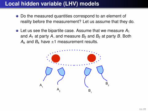
Do the measured quantities correspond to an element ofreality before the measurement? Let us assume that they do.

Let us see the bipartite case. Assume that we measure A1

and A1 at party A , and measure B2 and B2 at party B . BothAk and Bk have ±1 measurement results.

A1

A2 B

1

B2

11 / 77

Local hidden variable (LHV) models II

Ak and Bk are quantum mechanically incompatible.

Let us assume that all the four measurement outcomes existbefore the measurement.

The idea is that at each measurement k , there area1,k , a2,k , b1,k , b2,k available.

We expect a measurement record like the following:k a1,k a2,k b1,k b2,k

1 +1 −1 +1 +12 −1 +1 +1 −13 +1 +1 −1 +14 −1 −1 +1 −15 +1 +1 +1 −16 −1 −1 −1 +1... ... ... ... ...

Red color indicatesthe measured values.

12 / 77

Local hidden variable (LHV) models III

The correlations can be obtained as

〈AmBn〉 =1M

M∑k=1

am,k bn,k .

Here, k is the hidden variable.

Usual formula, with λ as a hidden variable

f(am, bn) =

∫fm,λ(am)gn,λ(bn)dλ

Here f ’s and g′s are probability density functions.

In words: all two-variable probability distributions can be givenas a sum of product distributions.

13 / 77

Bipartite nonlocality

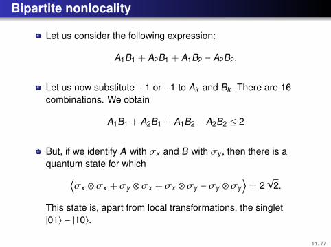
Let us consider the following expression:

A1B1 + A2B1 + A1B2 − A2B2.

Let us now substitute +1 or −1 to Ak and Bk . There are 16combinations. We obtain

A1B1 + A2B1 + A1B2 − A2B2 ≤ 2

But, if we identify A with σx and B with σy , then there is aquantum state for which⟨

σx ⊗ σx + σy ⊗ σx + σx ⊗ σy − σy ⊗ σy

⟩= 2√

2.

This state is, apart from local transformations, the singlet|01〉 − |10〉.

14 / 77

Bipartite nonlocality II

The real measurement record is the following:k a1,k a2,k b1,k b2,k

1 +1 ... +1 ...

2 −1 ... ... −13 ... +1 −1 ...

4 −1 ... +1 ...

5 ... +1 ... −16 −1 ... −1 ...

... ... ... ... ...

Red color indicatesthe measured values.

The correlations can be obtained as

〈AmBn〉 =1

|Mm,n |

∑k∈Mm,n

am,k bn,k ,

whereMm,n contains the indices corresponding to measuringAm and Bn. This is the reason that correlations do not fit anLHV model.

15 / 77

Bipartite nonlocality III

DefinitionBell inequalities are inequalities with correlation terms that areconstructed to exclude LHV models. They have the form

〈B〉 ≤ const.,

where B is the Bell operator.

One of the first one was the CHSH inequality,

A1B1 + A2B1 + A1B2 − A2B2 ≤ 2.

DefinitionThe visibility of a Bell inequality is defined as

V(B) =maxΨ 〈B〉Ψ

maxLHVB.

16 / 77

Convex sets: Correlations compatible with LHVmodels

The points corresponding to correlations fulfilling Bellinequalities are within a polytope. Extreme points havecorrelations ±1.

+1

-1

+1-1

⟨ A1B2 ⟩

⟨ A1 B1 ⟩

⟨ A2 B1 ⟩=1

⟨ A2 B2 ⟩=1

17 / 77

Outline




18 / 77

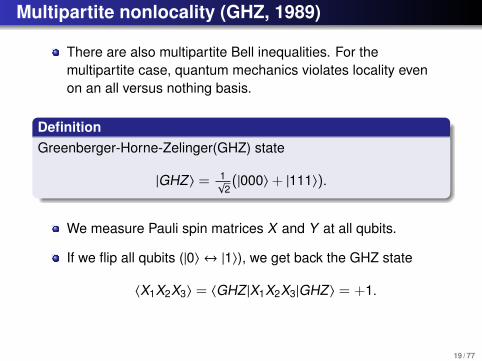
Multipartite nonlocality (GHZ, 1989)

There are also multipartite Bell inequalities. For themultipartite case, quantum mechanics violates locality evenon an all versus nothing basis.

DefinitionGreenberger-Horne-Zelinger(GHZ) state

|GHZ〉 = 1√2

(|000〉+ |111〉).

We measure Pauli spin matrices X and Y at all qubits.

If we flip all qubits (|0〉 ↔ |1〉), we get back the GHZ state

〈X1X2X3〉 = 〈GHZ |X1X2X3|GHZ〉 = +1.

19 / 77

Multipartite nonlocality (GHZ, 1989) II

If we flip one qubit (|0〉 ↔ |1〉) and apply flip+phase shift forthe other two, we get back the GHZ state

〈X1Y2Y3〉 = 〈GHZ |X1Y2Y3|GHZ〉 = −1.

We also have 〈Y1X2Y3〉 = 〈Y1Y2X3〉 = −1.

Based on common sense we would expect

X1X2X3 = (Y1Y2X3)(Y1X2Y3)(X1Y2Y3) = −1(wrong)

However, this is wrong. 〈X1X2X3〉 = +1 for the GHZ state.

Not only statistical contradiction. All experiments contradictthe assumption of an LHV model.[D. M. Greenberger, M. Horne, and A. Zeilinger, 1989.]

20 / 77

Mermin’s inequality (N.D. Mermin, PRL 1990)

For N qubits, the Mermin inequality is given by∑π

〈X1X2X3X4X5 · · · XN〉 −∑π

〈Y1Y2X3X4X5 · · · XN〉

+∑π

〈Y1Y2Y3Y4X5 · · · XN〉 − ... + ... ≤ LMermin,

where∑π represents the sum of all possible permutations of the

qubits that give distinct terms.

LMermin is the maximum for local states. It is defined as

LMermin =

{2N/2 for even N,2(N−1)/2 for odd N.

The quantum maximum is 2N−1.

21 / 77

Mermin’s inequality II

The visibility is increases exponentially with the number ofqubits:

VMermin =

{2N/2−1 for even N,2N/2−1/2 for odd N.

22 / 77

Ardehali’s inequality (M. Ardehali, PRA 1992)

DefinitionThe Ardehali inequality

〈(A (+)1 − A (−)

1 )(−

∑π

X2X3X4X5 · ·XN +∑π

Y2Y3X4X5 · ·XN

−∑π

Y2Y3Y4Y5X6 · ·XN + ... − ...)〉

+〈(A (+)1 + A (−)

1 )(∑

π

Y2X3X4X5 · ·XN −∑π

Y2Y3Y4X5 · ·XN

+∑π

X2Y3Y4Y5Y6X7 · ·XN − ... + ...)〉 ≤ LArdehali,

where A (±)1 are operators corresponding to measuring the first spin

along directions corresponding to the quantum operatorsA (±)

1 = (∓X1 − Y1)/√

2.

23 / 77

Ardehali’s inequality II

The Ardehali’s inequality is again maximally violated by theGHZ state.

The constant is

LArdehali =

{2N/2 for even N,2(N+1)/2 for odd N.

The quantum maximum is 2N−1 ×√

2 = 2N−1/2.

The visibility increases exponentially with the number ofqubits:

VArdehali =

{2N/2−1/2 for even N,2N/2−1 for odd N.

Remember:

VMermin =

{2N/2−1 for even N,2N/2−1/2 for odd N.

24 / 77

Bell inequalities with full correlation terms

DefinitionA full correlation term contains a variable for each spin.

X1Y2X3Y4 is a full correlation term

X1Y213X4 is not.

Among inequalities with full correlations terms, for any N, theMermin-Ardehali construction has the largest violationpossible.

The full set of such Bell inequalities can be written downconcisely in the form of a single nonlinear inequality. [R.F.Werner,

M.Wolf, PRA 2001; M. Zukowski, C. Brukner, PRL 2002.]

There are multi-qubit pure entangled states that do not violateany of these Bell inequalities. [M. Zukowski et al., PRL 2002.]

25 / 77

Not full correlation terms

It has been shown that such inequalities can detect any pureentangled multi-qubit state.[S. Popescu, D. Rohrlich, PLA 1992.]

Inequalities of this type can be constructed such that they aremaximally violated by cluster states and graph states. Inparticular, for the four-qubit cluster state this inequality lookslike

〈X112X3Z4〉+ 〈Z1Y2Y3Z4〉+ 〈X112Y3Y4〉 − 〈Z1Y2X3Y4〉 ≤ 2.

On all of the qubits two operators are measured except for thesecond qubit for which only Y2 is measured.

For a large class of graph states, e.g., for linear cluster states,it is possible to construct two-setting Bell inequalities thathave a visibility increasing exponentially with N. [O. Gühne et al., PRL

2005; G. Tóth et al., PRA 2006.]

26 / 77

Experiment

Figure: One of the two observer stations. All alignments andadjustments were pure local operations that did not rely on a commonsource or on communication between the observers.

[Figure from G. Weihs et al., Phys. Rev. Lett. 81 5039 (1998).]

27 / 77

Experiment II

0

200

400

600

800

1000 A+0/B–0 A+1/B–0

-100 -50 0 50 1000

200

400

600

800

Bias Voltage (Alice) [V]

A+0/B+0 A+1/B+0

Coi

ncid

ence

s in

5s

-0,50! -0,25! 0,00! 0,25! 0,50!Analyzer Rotation Angle

Figure: Four out of sixteen coincidence rates between various detectionchannels as functions of bias voltage (analyzer rotation angle) on Alice’smodulator. A+1/B−0 for example are the coincidences between Alice’s“+” detector with switch having been in position “1” and Bob’s “−”detector with switch position “0”. The difference in height can beexplained by different efficiencies of the detectors.

[Figure from G. Weihs et al., Phys. Rev. Lett. 81 5039 (1998).]

28 / 77

Outline




29 / 77

Wigner functions and LHV models

Is there a connection between other areas of physics andlocal hidden variable models?

Yes. For example, a surprising connection can be seen withWigner functions.

Wigner functions W(x, p) are defined for a single bosonicmodel such that

⟨(xmpn)sym

⟩=

∫xmpnW(x, p)dxdp.

The Wigner function is a quasi-probability distribution. That is∫W(x, p)dxdp = 1,

but W(x, p) can also be negative.

If W(x, p) ≥ 0 for all x and p, then it is a real probabilitydistribution.

30 / 77


Is there a connection between other areas of physics andlocal hidden variable models?Yes. For example, a surprising connection can be seen withWigner functions.


⟨(xmpn)sym

⟩=

∫xmpnW(x, p)dxdp.



If W(x, p) ≥ 0 for all x and p, then it is a real probabilitydistribution.

30 / 77


Is there a connection between other areas of physics andlocal hidden variable models?Yes. For example, a surprising connection can be seen withWigner functions.


⟨(xmpn)sym

⟩=

∫xmpnW(x, p)dxdp.



If W(x, p) ≥ 0 for all x and p, then it is a real probabilitydistribution. 30 / 77

Wigner functions and LHV models II

If W(x, p) ≥ 0 for all x and p, then it behaves as if there werea joint probability of the type

P(x0 ≤ x ≤ x0+dx, p0 ≤ p ≤ p0+dp) = W(x0, p0)dxdp (Wrong.)

In reality, this is not the case. If we measure x, to ask aboutthe value of p does not make sense, and vice versa.

If W(x, p) ≥ 0 for all x and p, then there is something like aLHV model for x and p. (However, note that they aremeasured on the same particle.)

31 / 77

Outline




32 / 77

What is new in a quantum system compared to itsclassical counterpart?

Let us compare a classical bit to a quantum bit (qubit)A classical bit is either in state "0" or in state "1".A qubit (two-state system) can be in a superposition of the two.

|Ψ〉 = c0|0〉+ c1|1〉,

where c0 and c1 are complex numbers. It is usual to use theshorthand notation, write

|Ψ〉 =

(c0

c1

),

and call |Ψ〉 the state vector.

To describe a quantum system one needs more degrees offreedom.

33 / 77

Two qubits

Let us consider a two-qubit system. Naively, one could thinkthat

|Ψ1〉 = c0|0〉+ c1|1〉,

|Ψ2〉 = d0|0〉+ d1|1〉,

However, the correct picture is that the two-qubit system isdescribed by

|Ψ12〉 = K0|00〉+ K1|01〉+ K2|10〉+ K3|11〉

where K ’s are complex constants.

Note that the number of the degrees of freedom in the secondcase is larger.

34 / 77

Two qubits II

The naive picture assumes that the two systems are in acertain quantum state independently of the other system.

There are quantum states like that, for example,

|Ψ1〉 = 1√2|0〉+ 1√

2|1〉,

|Ψ2〉 = 1√2|0〉+ 1√

2|1〉,

corresponds to

|Ψ12〉 = |Ψ1〉 ⊗ |Ψ2〉

=(

1√2|0〉+ 1√

2|1〉) ⊗ ( 1√

2|0〉+ 1√

2|1〉

)= 1

4

(|00〉+ |01〉+ |10〉+ |11〉

).

These are the product states that are examples of separablestates.

States that cannot be written in this product form are theentangled states.

35 / 77

Mixed states

So far we were talking about pure quantum states.

In a real experiment quantum states are mixed. Such statescan be described by a density matrix

ρ =∑

k

pk |Ψk 〉(|Ψk 〉)† =

∑k

pk |Ψk 〉〈Ψk |,

where∑

k pk = 1 and pk ≥ 0.

DefinitionA mixed state is separable if it can be written as the convexcombination of product states

ρ =∑

k

pkρ(1)k ⊗ ρ

(2)k .

Otherwise the state is entangled. [R. Werner, Phys. Rev. A 1989.]

36 / 77

Convexity

Properties of density matrices

ρ = ρ†,

Tr(ρ) = 1,

ρ ≥ 0.

Mixing two systems:

ρ′ = pρ1 + (1 − p)ρ2.

The set of density matrices is convex. If ρ1 and ρ2 are densitymatrices then ρ′ is also a density matrix.

The set of density matrices corresponding to separable statesis also convex. If ρ1 and ρ2 are separable density matricesthen ρ′ is also a separable density matrix.

37 / 77

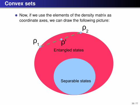
Convex sets

Now, if we use the elements of the density matrix ascoordinate axes, we can draw the following picture:

Separable states

Entangled states

ρ1

ρ2

ρ'

38 / 77

Convex sets II

A more correct figure is the following:

All quantum states (convex set)

Boundary: Densitymatrices with lessthan full rank

Boundary: Densitymatrices with lessthan full rank

Not only curved boundaries

Non-full rank density matrices have a zero eigenvalue. For atwo-state system, the pure states are on the boundary. 39 / 77

Convex sets III

A more correct figure for both sets is the following:

Pure product statesare at the boundaryof both sets

Separable states

All quantum states

40 / 77

Entanglement cannot be created locally

Remember: The definition of a separable state is

ρ =∑

k

pkρ(1)k ⊗ ρ

(2)k .

DefinitionLocal Operation and Classical Communications (LOCC):

Single-party unitaries,

Single party von Neumann measurements,

Single party POVM measurements,

We are even allowed to carry out measurement on party 1and depending on the result, perform some other operation onparty 2 ("Classical Communication").

LOCC and entanglement

It is not possible to create entangled states from separable states,with LOCC.

41 / 77

Entanglement is a resource

In short: Starting from a separable state, we cannot createentanglement without real two-party quantum dynamics.

In some cases such dynamics is impossible. For example, ifwe talk about particles very far away from each other.

Then, we can transform entangled states to other entangledstates, but cannot start from separable states and obtainentangled states.

Thus, entangled states are a resource in this case.

42 / 77

Why is entanglement important?

Can be used for quantum information processing protocols,quantum teleportation or quantum cryptography.

Important for quantum algorithms such as prime factoring orsearch.

Can also be used in quantum metrology (i.e., atomic clocks).

Entanglement is a natural goal for experiments.

43 / 77

Entanglement distillation

From many entangled particle pairs we want to create fewerstrongly entangled pairs with LOCC.

Strongly entangled

Strongly entangled

Entangled

Entangled

Entangled

Entangled

44 / 77

Entanglement of distillation and entanglement offormation

For the case of two-qibit, typically the aim is to create singletsthat are maximally entangled states.

|Ψsinglet〉 =1√

2(|01〉 − |10〉).

DefinitionThe entanglement of distillation a quantum state is characterizedby determining, how many singlets can be distilled from it byLOCC.

One can ask the opposite question. How many singlets areneeded to construct a quantum state. item

DefinitionThe entanglement of formation a quantum state is characterizedby determining, how many singlets are needed to form the state byLOCC. 45 / 77

Entanglement of distillation and entanglement offormation II

For pure states, the entanglement of formation equals the vonNeumann entropy of the reduced state

EF = −Tr(ρ1 log2 ρ1).

In general, the entanglement of formation is not smaller thanthe entanglement of distillation

EF ≥ ED .

DefinitionThere are entangled quantum states, that need singlets to createthem, but no singlets can be distilled by LOCC. These are calledbound entangled states.

46 / 77

Entanglement criteria

How to decide whether a quantum state with a given densitymatrix is entangled?

For pure states it is simple. A pure state is entangled if it is nota product state.

A mixed state is entangled if it cannot be written as

ρ =∑

k

pkρ(1)k ⊗ ρ

(2)k .

But how can we find out whether a quantum state can bedecomposed like that?

47 / 77

The positivity of the partial transpose (PPT) criterion

DefinitionFor a separable state %, the partial transpose is always positivesemidefinite

%T1 ≥ 0.

If a state does not have a positive semidefinite partial transpose,then it is entangled. [A. Peres, PRL 1996; Horodecki et al., PLA 1997.]

Partial transpose means transposing according to one of thetwo subsystems.

For separable states

(T ⊗ 1)% = %T1 =∑

k

pk (%(1)k )T ⊗ %

(2)k ≥ 0.

48 / 77

The positivity of the partial transpose (PPT) criterionII

How to obtain the partial transpose of a general densitymatrix? Example: 3 × 3 case.

Strongly entangled

Strongly entangled

EntangledEntangled

Entangled

Entangled

ϱ=

00 01 02 10 11 12 20 21 22

00

01

02

10

11

12

20

21

22

49 / 77

PPT entangled states are bound entangled

The PPT criterion detects all entangled states for 2 × 2 and2 × 3 systems.

For larger systems, it does not detect all entangled states.E.g., for 3x3 systems there are PPT entangled states.

It can be shown that no entanglement can be distilled fromthem, thus they are bound entangled.

50 / 77

The Computable Cross Norm-Realignment Criterion

DefinitionLet us consider a quantum state %, with a Schmidt decomposition

% =∑

k

λk G(A)k ⊗ G(B)

k ,

where Tr(G(l)m G(l)

n ) = δmn and λk ≥ 0. If % is separable then∑k λk ≤ 1.

[O. Rudolph, Quant. Inf. Proc. 2005; K. Chen and L.A. Wu, Quant. Inf. Comp. 2003.]

Proof. For product states the Schmidt decomposition of thedensity matrix is

%product = |ΨA 〉〈ΨA | ⊗ |ΨB〉〈ΨB |.

51 / 77

The Computable Cross Norm-Realignment Criterion II

For mixed states, we have to use that∑k

λk

defines a norm for quantum states that is convex.

Other definition of CCNR criterion is based on a "realignment"of the density matrix.

52 / 77

Entanglement detection with uncertainty relations

We have a bipartite system and the following operatorsA1 and B1 act on the first party.

A2 and B2 act on the second party.

If for quantum states

(∆Ak )2 + (∆Bk )2 ≥ c,

then for separable states we have

(∆A1 + A2)2 + (∆B1 + B2)2 ≥ 2c.

[ H.F. Hofmann and S. Takeuchi PRA 2003; O. Gühne, PRL 2004. ]

53 / 77

Entanglement detection with uncertainty relations II

Proof: For product states

|Ψ〉 = |Ψ1〉 ⊗ |Ψ2〉

we have

(∆(A1 + A2))2 + (∆(B1 + B2))2 =

(∆A1)2Ψ1

+ (∆B1)2Ψ1

+ (∆A2)2Ψ2

+ (∆B2)2Ψ2≥ 2c.

Separable states are mixtures of pure states. Due to convexitythis bound is also valid for separable states.

Simple example for two-mode systems

(∆(x1 + x2))2 + (∆(p1 − p2))2 ≥ 2.

54 / 77

Entanglement detection with a single nonlocalmeasurement: Entanglement witnesses

An operator W is an entanglement witness if〈W〉 = Tr(Wρ) < 0 only for entangled states.[Horodecki et al., Phys. Lett. A 223, 8 (1996); Terhal, quant-ph/9810091; Lewenstein, Phys. Rev. A 62, 052310

(2000).]

55 / 77

Entanglement vs. Nonlocality

All states that violate a Bell inequality are entangled.

Equivalently, separable states do not violate any Bellinequality.

However, there are entangled states that do not violate anyBell inequality. [R.F. Werner, PRA 1989.]

It is conjectured by Peres that every PPT state is local. Sofarno counterexamples have been found.

56 / 77

Entanglement vs. Nonlocality

The relations of the various convex sets look like as follows

Nonlocal entangled states

NPT ent. local states

Separable states

PPT ent. states

57 / 77

Outline




58 / 77

Many-body quantum systems

An N-qubit mixed state is separable if it can be written as

ρ =∑

k

pkρ(1)k ⊗ ρ

(2)k ⊗ ρ

(3)k ⊗ ... ⊗ ρ

(N)k .

Otherwise the state is entangled.

A bipartite quantum state is either separable or entangled.The multipartite case is more complicated.

We have to distinguish between quantum states in which onlysome of the qubits are entangled from those in which all thequbits are entangled.

Biseparable states are the states that might be entangled butthey are separable with respect to some partition. States thatare not biseparable are called genuine multipartite entangled.

59 / 77

Genuine multipartite entanglement

Let us see two entangled states of four qubits:

|GHZ4〉 = 1√2

(|0000〉+ |1111〉),

|ΨB〉 = 1√2

(|0000〉+ |0011〉) = 1√2|00〉 ⊗ (|00〉+ |11〉).

The first state is genuine multipartite entangled, the secondstate is biseparable.

60 / 77

Convex sets for the multi-qubit case

The idea also works for the multi-qubit case: A state isbiseparable if it can be composed by mixing pure bisparablestates.

Genuine multipartite entangled states

Separable states

Biseparable states

61 / 77

Outline




62 / 77

Detection of entanglement

Many quantum engineering/quantum control experimentshave two main steps:

Creation of an entangled quantum state,Detection its entanglement.

Thus entanglement detection is one of the most importantsubjects in this field.

Examples of quantum control experiments:Nuclear spin of atoms in a molecule (NMR): ≤ 10 qubitsParametric down-conversion and post-selection: ≤ 10 qubitsTrapped ion experiments: ≤ 8 qubits

63 / 77

Entanglement detection with tomography

Determine the density matrix and apply an entanglementcriterion.

For N qubits the density matrix has 2N × 2N complexelements, and has 22N − 1 real degrees of freedom.

10 qubits→ ∼ 1 million measuremets20 qubits→ ∼ 1012 measuremets

Surprise: Above modest system sizes full tomography is notpossible. One has to find methods for entanglement detectionthat are feasible even without knowing the quantum state.

64 / 77

Entanglement detection with a single nonlocalmeasurement: Entanglement witnesses

An operator W is an entanglement witness if〈W〉 = Tr(Wρ) < 0 only for entangled states.[Horodecki et al., Phys. Lett. A 223, 8 (1996); Terhal, quant-ph/9810091; Lewenstein, Phys. Rev. A 62, 052310

(2000).]

Separable states

Entangled states

Quantum states detected by the witness

65 / 77

Entanglement detection with local measurements

Example:

WGHZ :=121 − |GHZ〉〈GHZ |

is a witness, where |GHZ〉 := (|000..00〉+ |111..11〉)/√

2.WGHZ detects entanglement in the vicinity of GHZ states.

Problem: Only local measurements are possible. With localmeasurements, operators of the type 〈A (1)B(2)C(3)C(4)〉 canbe measured.

A B C D

Qubit #1

Qubit #2

Qubit #3

Qubit #4

66 / 77

Entanglement detection with local measurements II

All operators must be decomposed into the sum of locallymeasurable terms and these terms must be measuredindividually.

For example,

|GHZ3〉〈GHZ3| =18

(1 + σ(1)z σ

(2)z + σ

(1)z σ

(3)z + σ

(2)z σ

(3)z )

+14σ

(1)x σ

(2)x σ

(3)x )

−116

(σ(1)x + σ

(1)y )(σ

(2)x + σ

(2)y )(σ

(3)x + σ

(3)y )

−116

(σ(1)x − σ

(1)y )(σ

(2)x − σ

(2)y )(σ

(3)x − σ

(3)y ).

[O. Gühne és P. Hyllus, Int. J. Theor. Phys. 42, 1001-1013 (2003). M. Bourennane et al., Phys. Rev. Lett. 92

087902 (2004).]

As N increases, the number of terms increases exponentially.

67 / 77

Solution: Entanglement witnesses designed fordetection with few measurements

Alternative witness with easy decomposition

W ′GHZ := 31 − 2

[σ

(1)x σ

(2)x · · · σ

(N−1)x σ

(N)x

2+

N∏k=2

σ(k)z σ

(k+1)z + 1

2

].

Note that W ′GHZ ≥ 2WGHZ . [GT and O. Gühne, Phys. Rev. Lett. 94, 060501 (2005).]

The number of local measurements does not increases withN.

σx

σx σ

xσx

σz

σz σ

zσz

1.

2.

68 / 77

Example: An experiment

Creation of a four-qubit cluster state with photons and itsdetection [Figure from Kiesel, C. Schmid, U. Weber, GT, O. Gühne, R. Ursin, and H. Weinfurter, Phys.

Rev. Lett. 95, 210502; See also GT and O. Gühne, Phys. Rev. Lett. 94, 060501 (2005).]

PDBS

a

b'

PBS

c'

UV pulses

type IISPDC

BBO

HWP

M

F

PDBS PDBS

QWP

T = 1/3T = 1H

V

T = 1/3T = 1H

V

1

2 3T = 1

T = 1/3H

V

d

C-Phase Gate

cb

69 / 77

Outline




70 / 77

Very many particles

Typically we cannot address the particles individually.

Expected to occur often in future experiments.

For spin-12 particles, we can measure the collective angular

momentum operators:

Jl := 12

N∑k=1

σ(k)l ,

where l = x, y, z and σ(k)l a Pauli spin matrices.

We can also measure the (∆Jl)2 := 〈J2

l 〉 − 〈Jl〉2 variances.

71 / 77

Spin squeezing I.

Uncertainty relation for the spin coordinates:

(∆Jx)2(∆Jy)2 ≥ 14 |〈Jz〉|

2.

If (∆Jx)2 is smaller than the standard quantum limit 12 |〈Jz〉|

then the state is called spin squeezed.[ M. Kitagawa and M. Ueda, Phys. Rev. A 47, 5138 (1993).]

Application: Quantum metrology.

Jz is large

Variance of Jx is small

z

yx

72 / 77

Spin squeezing II.

Spin squeezing experiment with 107 atoms: [J. Hald, J. L. Sørensen, C.

Schori, and E. S. Polzik, Phys. Rev. Lett. 83, 1319 (1999)]

Spin squeezing criterion for the detection of quantumentanglement

(∆Jx)2

〈Jy〉2 + 〈Jz〉

2≥

1N.

If a quantum state violates this criterion then it is entangled.[A. Sørensen et al., Nature 409, 63 (2001).]

73 / 77

Generalized spin squeezing criteria

Criterion 1. For separable states we have

〈J2x 〉+ 〈J2

y 〉 ≤N4

(N + 1).

This detects entangled states close to symmetric Dicke states〈Jz〉 = 0. E.g., for N = 4-re this state is

1√6

(|0011〉+ |0101〉+ |1001〉+ |0110〉+ |1010〉+ |1100〉).[GT, J. Opt. Soc. Am. B 24, 275 (2007); N. Kiesel et al., Phys. Rev. Lett. 98, 063604 (2007).]

Criterion 2. For separable states

(∆Jx)2 + (∆Jy)2 + (∆Jz)2 ≥ N/2.

The left hand side is zero for the ground state of a Heisenbergchain. [GT, Phys. Rev. A 69, 052327 (2004).]

Criterion 3. For symmetric separable states1 − 4〈Jm〉

2/N2 ≤ 4(∆Jm)2/N. [J. Korbicz et al. Phys. Rev. Lett. 95, 120502 (2005).]

How could we find all such criteria?74 / 77

Complete set of generalized spin squeezinginequalities

Let us assume that for a system we know only

J := (〈Jx〉, 〈Jy〉, 〈Jz〉),

K := (〈J2x 〉, 〈J

2y 〉, 〈J

2z 〉).

Then any state violating the following inequalities is entangled

〈J2x 〉+ 〈J2

y 〉+ 〈J2z 〉 ≤ N(N + 2)/4,

(∆Jx)2 + (∆Jy)2 + (∆Jz)2 ≥ N/2,

〈J2k 〉+ 〈J2

l 〉 − N/2 ≤ (N − 1)(∆Jm)2,

(N − 1)[(∆Jk )2 + (∆Jl)

2]≥ 〈J2

m〉+ N(N − 2)/4,

where k , l,m takes all the possible permutations of x, y, z.[GT, C. Knapp, O. Gühne, és H.J. Briegel, Phys. Rev. Lett. 2007.]

75 / 77

The polytope

The previous inequalities, for fixed 〈Jx/y/z〉, describe apolytope in the 〈J2

x/y/z〉 space.

Separable states correspond to points inside the polytope.Note: Convexity comes up again!

For 〈J〉 = 0 and N = 6 the polytope is the following:

05

10

0

5

10

0

5

10

⟨ J2y ⟩

⟨ J2x ⟩

⟨ J2 z ⟩

Az

Ay

Ax

Bx

Bz

By

S

76 / 77

Conclusions

We discussed Bell inequalities and local hidden variablemodels

We discussed separability and entanglement.

We also discussed entanglement criteria and entanglementdetection in experiments.

For further information please see my home page:

http://optics.szfki.kfki.hu/∼toth

and the review

O. Gühne and G. Tóth, Physics Reports 474, 1-75 (2009).

*** THANK YOU ***

77 / 77

http://www.szfki.kfki.hu/~toth

quantum entanglement and its detection with few …outline 1 introduction 2 nonlocality, bell...

Documents