quantum chemistry for spectroscopy { a tale of...
TRANSCRIPT
Quantum Chemistry for Spectroscopy – A Tale of
Three Spins (S = 0, 12, and 1)
by
Bryan Matthew Wong
Submitted to the Department of Chemistryin partial fulfillment of the requirements for the degree of
Doctor of Philosophy
at the
MASSACHUSETTS INSTITUTE OF TECHNOLOGY
May 2007
c© Massachusetts Institute of Technology 2007. All rights reserved.
Author . . . . . . . . . . . . . . . . . . . . . . . . . . . . . . . . . . . . . . . . . . . . . . . . . . . . . . . . . . . . . .Department of Chemistry
May 18, 2007
Certified by. . . . . . . . . . . . . . . . . . . . . . . . . . . . . . . . . . . . . . . . . . . . . . . . . . . . . . . . . .Robert W. Field
Haslam and Dewey Professor of ChemistryThesis Supervisor
Accepted by . . . . . . . . . . . . . . . . . . . . . . . . . . . . . . . . . . . . . . . . . . . . . . . . . . . . . . . . .Robert W. Field
Chairman, Department Committee on Graduate Students

This doctoral thesis has been examined by a Committee of the Department of
Chemistry that included
Professor Jianshu Cao
(Chairperson)
Professor Troy Van Voorhis
Professor Robert W. Field
(Thesis Supervisor)
2

Quantum Chemistry for Spectroscopy – A Tale of Three
Spins (S = 0, 12, and 1)
by
Bryan Matthew Wong
Submitted to the Department of Chemistryon May 18, 2007, in partial fulfillment of the
requirements for the degree ofDoctor of Philosophy
Abstract
Three special topics in the field of molecular spectrocopy are investigated using avariety of computational techniques. First, large-amplitude vibrational motions onground-state singlet (S0) potential energy surfaces are analyzed for both the acety-lene/vinylidene and the HCN/HNC isomerization systems. Electronic properties suchas electric dipole moments and nuclear quadrupole coupling constants are used asdiagnostic markers of progress along the isomerization path. Second, the topic ofelectronically excited triplet states and their relevance to doorway-mediated intersys-tem crossing for acetylene is considered. A new diabatic characterization of the thirdtriplet electronic state, T3, enables a vibrational analysis of data obtained from currentand past experiments. The last part of this thesis reviews the techniques and ideasof electron-molecule collisions relevant to Rydberg states of diatomic molecules. Pre-viously developed and current methods of treating the excited Rydberg electron areevaluated and extended. Each of these three topics in molecular spectroscopy is stud-ied using ab initio approaches coupled with experimental observations or chemicallyintuitive models. The unique combination of quantum chemistry and spectroscopystimulates further developments in both theory and experiment.
Thesis Supervisor: Robert W. FieldTitle: Haslam and Dewey Professor of Chemistry
3

4

Acknowledgments
It is a pleasure to thank those people who have helped me with various aspects of this
thesis. First and foremost, I want to express my gratitude to Prof. Robert W. Field
for devoting an enormous investment of time and patience to teaching me about the
spectroscopy of small molecules. I would like to thank Bob for constantly reminding
me that there is often simplicity behind every complexity. His invaluable view and
intuition has improved this work in many ways.
In addition, several colleagues have provided support in both professional and
personal capacities. Adam H. Steeves deserves recognition for writing most of the J.
Phys. Chem. B manuscript on large-amplitude motions of S0 acetylene. Additionally,
Dr. Hans A. Bechtel was always available to explain and provide the HCN/HNC
nuclear quadrupole coupling constants measured from his experiments. I also owe
both Adam and Hans a non-research related acknowledgement for helping me “find
Aerosmith” (on two separate occasions) for my computer. I acknowledge Dr. Ryan
L. Thom and Prof. John F. Stanton for teaching me about excited states of triplet
acetylene. I would also like to thank John for several helpful lessons (in the great state
of Texas) on obtaining diabatic parameters from quantum chemistry calculations.
Dr. Serhan N. Altunata and Dr. Stephen L. Coy deserve credit for introducing
me to electron-molecule scattering techniques. I thank Serhan for explaining the
methodological subtleties of scattering theory to me whenever I required his help. I
am grateful to Kyle L. Bittinger for extremely qualified help with writing programs
in perl. An advantage of working in the Field group is the variety of science that
I learned, and I would like to thank all the other group members at M.I.T. during
my stay. I would like to express particular thanks to Dr. Kate L. Bechtel and
Samuel H. Lipoff for their support during and after my thesis defense. Sam organized
the celebration after my thesis defense, and Kate wore the M.I.T. beaver mascot
costume during my entire thesis defense (it gets very hot in that furry costume).
Their encouragement is greatly appreciated.
My last few years at M.I.T. were particularly difficult, and it is appropriate to
5

express my gratitude to those who prayed for me and gave me invaluable advice. Dr.
Sumathy Raman, Dr. Oleg A. Mazyar, and Dr. Andrei A. Golosov all helped me fig-
ure out what I should do during these years and what my future plans should be after
my time at M.I.T. I am grateful that they also remain close scientific collaborators.
Finally, the completion of my education at M.I.T. would not have been possible with-
out my family. Although they did not help me with the scientific details of singlet,
triplet, or Rydberg states, they did something far better. They constantly prayed for
me and supported me, even when I did not have confidence in myself. Extra special
thanks goes to Mom, Dad, and my sister, Bonnie.
6

To my family: Mom, Dad, and Bonnie
7

8

Contents
1 Introduction 23
1.1 Motivation . . . . . . . . . . . . . . . . . . . . . . . . . . . . . . . . . 23
1.2 Outline . . . . . . . . . . . . . . . . . . . . . . . . . . . . . . . . . . . 24
2 One-Dimensional Molecular Hamiltonians 29
2.1 Introduction . . . . . . . . . . . . . . . . . . . . . . . . . . . . . . . . 29
2.2 Hamiltonian . . . . . . . . . . . . . . . . . . . . . . . . . . . . . . . . 31
2.3 Eckart Reduced Inertias . . . . . . . . . . . . . . . . . . . . . . . . . 35
2.4 Pitzer Reduced Inertias . . . . . . . . . . . . . . . . . . . . . . . . . . 37
2.5 Examples and Applications . . . . . . . . . . . . . . . . . . . . . . . 39
2.6 Conclusion . . . . . . . . . . . . . . . . . . . . . . . . . . . . . . . . . 46
3 Electronic Signatures of Large-Amplitude Motion in S0 Acetylene 49
3.1 Introduction . . . . . . . . . . . . . . . . . . . . . . . . . . . . . . . . 49
3.2 Hamiltonian . . . . . . . . . . . . . . . . . . . . . . . . . . . . . . . . 52
3.3 Ab Initio Calculations . . . . . . . . . . . . . . . . . . . . . . . . . . 55
3.4 Dipole Moments in the Unsymmetrized Local Mode Basis . . . . . . . 60
3.5 Local Bending in the Polyad Model . . . . . . . . . . . . . . . . . . . 62
3.6 Results . . . . . . . . . . . . . . . . . . . . . . . . . . . . . . . . . . . 62
3.7 Evolution of the Dipole Moment . . . . . . . . . . . . . . . . . . . . . 64
3.8 Assignment of Large-Amplitude Local Bender States . . . . . . . . . 67
3.9 Conclusions . . . . . . . . . . . . . . . . . . . . . . . . . . . . . . . . 70
9

4 The Hyperfine Structure of HCN and HNC 71
4.1 Introduction . . . . . . . . . . . . . . . . . . . . . . . . . . . . . . . . 71
4.2 Quadrupole Coupling Constants of Nuclei . . . . . . . . . . . . . . . 73
4.3 Application to the HCN HNC Isomerization System . . . . . . . . 75
4.4 Results for HCN and HNC . . . . . . . . . . . . . . . . . . . . . . . . 78
4.5 Conclusion . . . . . . . . . . . . . . . . . . . . . . . . . . . . . . . . . 83
5 Valence-Excited States of Triplet Acetylene 85
5.1 Introduction . . . . . . . . . . . . . . . . . . . . . . . . . . . . . . . . 85
5.2 Previous Studies on Triplet Acetylene . . . . . . . . . . . . . . . . . . 87
5.3 A New Ab Initio Study of the T3 Surface . . . . . . . . . . . . . . . . 90
5.4 A Brief Digression on Adiabatic and Diabatic Representations . . . . 92
5.5 The T2/T3 Vibronic Model . . . . . . . . . . . . . . . . . . . . . . . . 96
5.6 S1/T3 Vibrational Overlap Integrals . . . . . . . . . . . . . . . . . . . 99
5.7 Results for T3 Acetylene . . . . . . . . . . . . . . . . . . . . . . . . . 105
5.8 Conclusion . . . . . . . . . . . . . . . . . . . . . . . . . . . . . . . . . 109
6 Computational Techniques for Electron-Molecule Scattering 111
6.1 Introduction . . . . . . . . . . . . . . . . . . . . . . . . . . . . . . . . 111
6.2 Variational Derivation of the K matrix . . . . . . . . . . . . . . . . . 115
6.3 Numerical Evaluation of Integrals . . . . . . . . . . . . . . . . . . . . 120
6.4 Representing the Continuum Functions . . . . . . . . . . . . . . . . . 122
6.5 Additional Computational Details . . . . . . . . . . . . . . . . . . . . 124
6.6 Test Calculations on the 1sσg4pσu1Σ+
u State of H2 . . . . . . . . . . 126
6.7 Conclusion . . . . . . . . . . . . . . . . . . . . . . . . . . . . . . . . . 128
7 Developments in Electron Scattering for Polar Molecules 131
7.1 Introduction . . . . . . . . . . . . . . . . . . . . . . . . . . . . . . . . 131
7.2 The Electron Scattering Equations . . . . . . . . . . . . . . . . . . . 133
7.3 A Partial Differential Equation Approach . . . . . . . . . . . . . . . . 135
7.4 Boundary Conditions Adapted for Long Range Dipoles . . . . . . . . 139
10

7.5 The Finite Element Approach . . . . . . . . . . . . . . . . . . . . . . 145
7.6 Extracting the K matrix . . . . . . . . . . . . . . . . . . . . . . . . . 150
7.7 Conclusion . . . . . . . . . . . . . . . . . . . . . . . . . . . . . . . . . 151
8 Conclusion 153
8.1 Summary . . . . . . . . . . . . . . . . . . . . . . . . . . . . . . . . . 153
8.2 Future Directions . . . . . . . . . . . . . . . . . . . . . . . . . . . . . 154
A Expansion of the Internal Coordinate Hamiltonian 157
B Computer Codes for Calculating Vibrational Overlap Integrals 165
B.1 overlap integral.m . . . . . . . . . . . . . . . . . . . . . . . . . . . . . 165
B.2 make overlap table.m . . . . . . . . . . . . . . . . . . . . . . . . . . . 169
B.3 load acetylene data.m . . . . . . . . . . . . . . . . . . . . . . . . . . 171
B.4 b matrix acetylene.m . . . . . . . . . . . . . . . . . . . . . . . . . . . 176
C Analytical Expressions for One- and Two-Electron Integrals in K
matrix Calculations 179
C.1 General Expansion of Cartesian Gaussian Orbitals . . . . . . . . . . . 179
C.2 Overlap Integrals . . . . . . . . . . . . . . . . . . . . . . . . . . . . . 181
C.3 Kinetic Energy Integrals . . . . . . . . . . . . . . . . . . . . . . . . . 183
C.4 Nuclear Attraction Integrals . . . . . . . . . . . . . . . . . . . . . . . 183
C.5 Electron Repulsion Integrals . . . . . . . . . . . . . . . . . . . . . . . 185
11

12

List of Figures
2-1 Eckart effective inertias (Eq. (2.12)) for six molecules displaying in-
ternal rotation compared with those calculated from Pitzer’s formulae
(Eq. (2.19)). . . . . . . . . . . . . . . . . . . . . . . . . . . . . . . . . 42
2-2 The lowest 2,500 eigenvalues for the torsional motion of 1,2-dichloroethane.
The eigenvalues obtained from the instantaneous Eckart inertias are
considerably larger than those obtained from a constant-valued Pitzer
inertia at the trans geometry. . . . . . . . . . . . . . . . . . . . . . . 43
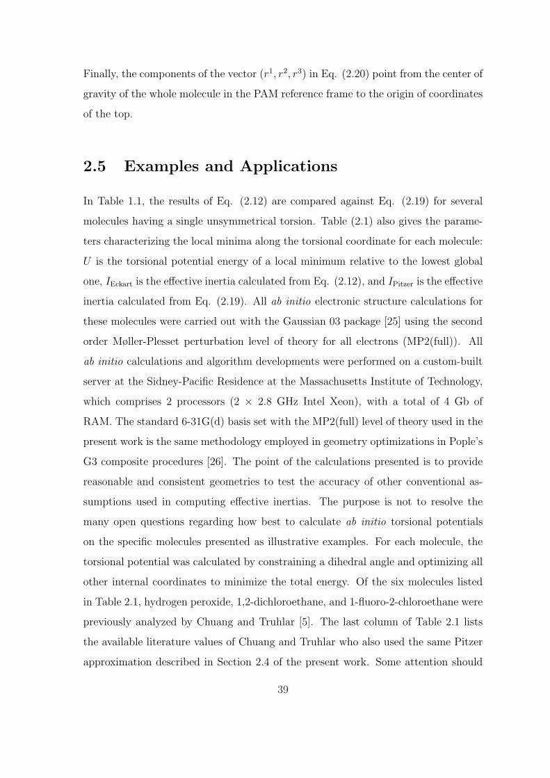
2-3 (a) Relaxed torsional potential and energies for 1,2-dichloroethane ob-
tained at the MP2(full)/6-31G(d) level of theory. Each of the tor-
sional eigenvalues is associated with symmetric (red-colored) and anti-
symmetric (green-colored) torsional states. (b) Torsionally averaged
Eckart inertias, 〈IEckart〉, for the lowest 150 torsional states of 1,2-
dichloroethane. The broken line indicates the numerical value of IPitzer
= 16.37 amu A2 calculated at the trans global minimum. . . . . . . . 44
2-4 Reduced moment of inertia calculated by the Powell dogleg algorithm
for the HCC bending motion of acetylene. The effective inertia in-
creases rapidly near 110 when the rightmost hydrogen moves in con-
cert with the leftmost hydrogen to form vinylidene. . . . . . . . . . . 45
13

3-1 (a) One-dimensional relaxed potential for the acetylene-vinylidene iso-
merization as a function of the HCC valence bend angle. A transi-
tion state structure is labeled by the number 2, and local minima are
denoted by numbers 3 and 4. (b) Spatial positions of the acetylene
coordinates color-coded to match their corresponding location on the
one-dimensional potential. The rightmost hydrogen retraces its path
near the transition state but moves in concert with the leftmost hydro-
gen in the red-colored post transition state 2 regions. . . . . . . . . . 50
3-2 Dipole moments computed for relaxed geometries as a function of (a)
fixed HCC local bend angle and (b) fixed local C–H stretch distance.
In Figure 3-2 (a), the schematic diagrams of the bending motion show
that when the local bend is excited, the b-axis dipole moment must
change sign at θ = 0. Conversely, the a-axis dipole moment is sym-
metric about θ = 0 since the active hydrogen is always placed at iden-
tical horizontal distances along the a-axis during the (symmetric) local
bending motion. In Figure 3-2 (b), the broken line indicates the nu-
merical value of the dipole moment for the CCH equilibrium geometry.
The dipole moments for Figures 3-2 (a) and (b) were obtained from
the CCSD/aug-cc-pVTZ and MR-AQCC/aug-cc-pVQZ levels of the-
ory, respectively. . . . . . . . . . . . . . . . . . . . . . . . . . . . . . 58
3-3 Experimentally derived polyad frequencies for a local CCH bending
motion compared with one-dimensional ab initio calculations. The fre-
quencies obtained from the polyad model and the ab initio calculations
intersect near 18 quanta of Nbend. Adam H. Steeves is acknowledged
for providing the polyad frequencies. . . . . . . . . . . . . . . . . . . 64
14
3-4 Vibrationally averaged ab initio dipole moments computed (a) for a
local C–H stretch and (b) for a local bend. Since the b-axis dipole
moment for the local bend is antisymmetric with respect to the equi-
librium bend angle, its vibrational average is exactly zero, and only
the vibrational average for the a-axis dipole is displayed. The bottom
axis of Figure 3-4 (b) is numbered according to the vibrational level
in the fully permutational symmetric isomerization path, and the top
axis labels only the symmetric vibrational levels. Both averaged dipole
moments are reported relative to the lowest vibrational quantum state. 65
4-1 Dipole moment as a function of the Jacobi angle (defined in Figure 4-3)
along an isomerization path from HCN (0) to HNC (180). Dipole mo-
ments were calculated at the CCSD(full) level with the aug-cc-pCVTZ
basis. . . . . . . . . . . . . . . . . . . . . . . . . . . . . . . . . . . . . 72
4-2 (a)–(c) Nuclear shapes and nuclear electric quadrupole moments. . . . 75
4-3 Jacobi coordinates for the HNC molecule. . . . . . . . . . . . . . . . 76
4-4 Dependence of the nuclear quadrupole coupling constant (eQq)N on a
relaxed HCN HNC isomerization path. . . . . . . . . . . . . . . . 77
4-5 Dependence of the nuclear quadrupole coupling constant (eQq)D on a
relaxed DC15N D15NC isomerization path. The arrows along the
horizontal axis indicate molecular geometries where (1) the D atom is
directly over the C atom (θ = 60), (2) the D atom is over the C–N
midpoint (θ = 90), and (3) the D atom is directly over the N atom
(θ = 117). . . . . . . . . . . . . . . . . . . . . . . . . . . . . . . . . . 78
4-6 (a) One-dimensional relaxed potential for the HCN HNC isomeriza-
tion as a function of the Jacobi angle. The transition state structure is
labeled by the number 2, and HCN/HNC minima are denoted by num-
bers 1 and 3, respectively. (b) Spatial positions of the the HCN/HNC
atoms color-coded to match their corresponding location on the one-
dimensional potential. . . . . . . . . . . . . . . . . . . . . . . . . . . 79
15

4-7 (a) The 50 lowest vibrational eigenvalues for the HCN HNC po-
tential obtained at the CCSD(T)/aug-cc-pVQZ level of theory. Each
of the eigenvalues is associated with either HCN (green-colored) or
HNC (red-colored) localization. (b) Vibrationally averaged nuclear
quadrupole coupling constants for the lowest 50 vibrational states of
HCN (green)/HNC (red) energy. . . . . . . . . . . . . . . . . . . . . . 80
4-8 Calculated and experimental (l = 0) vibrational frequencies for HCN
and HNC. The lines were fitted using a least squares method which
yields ab initio slopes of 710.8 cm−1/(HCN bend quantum) and 492.1
cm−1/(HNC bend quantum) and experimental slopes of 685.6 cm−1/(HCN
bend quantum) and 468.4 cm−1/(HNC bend quantum). . . . . . . . . 81
4-9 Calculated and experimental (l = 0) nuclear quadrupole coupling con-
stants for HCN and HNC. The lines were fitted using a least squares
method which yields ab initio slopes of -0.062 MHz/(HCN bend quan-
tum) and -0.157 MHz/(HNC bend quantum) and experimental slopes
of -0.075 MHz/(HCN bend quantum) and -0.118 MHz/(HNC bend
quantum). Dr. Hans A. Bechtel is acknowledged for providing the
experimental quadrupole coupling constants. . . . . . . . . . . . . . . 82
5-1 Highest occupied molecular orbital for the S11Au trans state of acetylene. 86
5-2 Potential energy curves for cis−trans bending calculated at the EOM-
CCSD level with the cc-pVTZ basis. The first excited electronic states
are stabilized by bending out of linearity. . . . . . . . . . . . . . . . . 87
5-3 Zeeman anticrossing spectra for the ν ′3 = 0− 3 vibrational levels of the
A 1Au state. An increase in the number of anticrossings is observed
with increasing excitation of the ν ′3 mode. Figures reproduced from
Ref. [1]. . . . . . . . . . . . . . . . . . . . . . . . . . . . . . . . . . . 88
5-4 The ν3 (ag) trans-bending normal mode for the A 1Au state of acety-
lene. The harmonic vibrational frequency was calculated at the EOM-
CCSD level with the cc-pVQZ basis. . . . . . . . . . . . . . . . . . . 89
16
5-5 (a) Potential energy curves as a function of the HCCH torsion and (b)
intersection of the T2/T3 surfaces as a function of the HCCH and CCH
angles under a C2 symmetry restriction. Energies for both figures were
calculated at the EOM-CCSD level with the cc-pVTZ basis. . . . . . 90
5-6 Highest occupied molecular orbital for the lowest stationary point on
T3 (3B). The geometry parameters for this C2 symmetry stationary
point are listed in Table 5.1. . . . . . . . . . . . . . . . . . . . . . . . 91
5-7 (a) The ν6 antisymmetric CCH bending normal mode for T3 acetylene
(∠H1C1C2 = θeq −∆θ, ∠H2C2C1 = θeq + ∆θ) and (b) adiabatic T2/T3
surfaces as a function of the HCCH torsional angle and CCH asymmet-
ric bend angle. The T2/T3 energies were obtained at the EOM-CCSD
level with the cc-pVTZ basis. The stationary point on T3 is unstable
against increasing ∆θ. . . . . . . . . . . . . . . . . . . . . . . . . . . 92
5-8 Representative adiabatic and diabatic potential energy curves as a
function of the normal coordinate q. The solid adiabatic curves are
separated by an energy difference of ∆ at q = 0, but the dotted dia-
batic curves are allowed to intersect. . . . . . . . . . . . . . . . . . . 93
5-9 (a)–(d) Adiabatic potential energy curves (Eq. (5.2)) as a function of
the normal coordinate q. All potential curves have identical values of
∆, ω1, and ω2. As the vibronic coupling parameter λ is increased, the
curves are better approximated in the diabatic representation. . . . . 94
5-10 Diabatic potential energy curves represented in the new basis of Eq.
(5.4). . . . . . . . . . . . . . . . . . . . . . . . . . . . . . . . . . . . . 95
5-11 (a)–(f) Diabatized vibrational normal modes for the T33B state. . . . 106
17

6-1 (a) Schematic picture of an excited Rydberg state with high angular
momentum, l. When an electron occupies a large Rydberg orbital,
the nuclear and electronic motions are largely separable. (b) Depiction
of a Rydberg state with low angular momentum. When the Rydberg
electron penetrates the ion core, it can exchange energy and angular
momentum with the nuclei. . . . . . . . . . . . . . . . . . . . . . . . 112
6-2 Schematic diagram of a molecule enclosed by a notional sphere of ra-
dius R. Exchange between the scattered and atomic electrons is only
important within the sphere. The bound wavefunctions centered on
nuclei ZA and ZB (only two nuclei are shown for clarity) have negligi-
ble amplitude outside the sphere. . . . . . . . . . . . . . . . . . . . . 113
6-3 (a)–(b) Analytical continuum functions fl(k, r) and(1− e−λrl+1
)gl(k, r)
with l = 1 (crosses). Each of the continuum functions are fit by a lin-
ear combination of 9 single-centered Gaussian functions (full curves)
for E = −0.03125 Hartrees. . . . . . . . . . . . . . . . . . . . . . . . 123
6-4 Potential energy curves for the H+2 ion ground state and the 1sσg4pσu
1Σ+u state of H2. Energies for the H+
2 ion were calculated at the ROHF
level with the 6-31G basis, and the solid energy curve is the result of
a high level ab initio calculation by Staszewska et al. [2]. The blue
data points were obtained from the two-electron K matrix calculation
described in this work. . . . . . . . . . . . . . . . . . . . . . . . . . . 127
7-1 CCSD(full) cc-pCVTZ electric dipole moments for the CaF+ ion com-
pared with those obtained from the effective potential of Ref. [3]. Both
the CCSD(full) and effective potential dipoles agree with each other
near the equilibrium internuclear distance (R = 3.54 Bohrs), but con-
siderable deviations are observed for small and large R. Dr. Stephen
L. Coy is acknowledged for providing the dipole moments from the
effective potential. . . . . . . . . . . . . . . . . . . . . . . . . . . . . 132
18

7-2 Coordinate system for a CaF+ ion used throughout Chapter 7. The
CaF+ ion is aligned along the z-axis with the origin at its center of
mass. The orientation of the z-axis is defined such that the dipole
moment points towards the positive z-axis. . . . . . . . . . . . . . . . 137
7-3 Values of leff (leff + 1), obtained from Eq. (7.27) as a function of the
dipole moment. The solid lines are eigenvalues for m = 0. The dashed
and dotted lines correspond to m = 1 and 2, respectively. For suffi-
ciently strong dipole moments, leff (leff + 1) will become negative. . . . 141
7-4 Angular plots of Re (Θ(θ)Φ(φ)) evaluated for a 8.6863 Debye dipole
at the origin. The negative z-axis corresponds to the position of a
negative partial charge. Figure 7-4 (a) depicts a 4sσ orbital which is
strongly polarized away from the negative charge, and (b) depicts a
4fφ orbital which resembles a hydrogenic orbital. . . . . . . . . . . . 142
7-5 Optimal values of α(rc) as a function of energy for a l = 1 Coulomb
potential. The circles at E > 0 were determined by integrating Eq.
(7.36) using the boundary conditions in Eqs. (7.37)–(7.38). The solid
curve is a spline fit to the circles only which smoothly extrapolates to
E < 0. . . . . . . . . . . . . . . . . . . . . . . . . . . . . . . . . . . . 144
7-6 (a) Deviations between a numerically calculated l = 2 Coulomb phase
β(E)/π and its analytical value ν − l. The dashed curve was obtained
using a WKB boundary condition to approximate α(rc) at the mini-
mum of the effective potential [4]. The solid curve was obtained from
the extrapolated boundary condition described in this chapter. (b)
Magnified plot of Figure 7-6 (a). . . . . . . . . . . . . . . . . . . . . . 145
19

7-7 (a) Four piecewise linear basis functions (solid lines) for the one-dimensional
finite element method. A linear combination of them is shown as a
broken line. (b) Piecewise linear basis functions in two dimensions. A
triangular mesh is plotted in the xy-plane, and the linear combination
of basis functions is plotted above it. (For the curious reader, Figure
7-7 (b) depicts a solution to the Helmholtz’s differential equation for
waves reflecting off a 0.1 × 0.1 square in the center.) . . . . . . . . . 146
7-8 (a) Boundary conditions for integrating Eqs. (7.22)–(7.23) using a
sparse finite element mesh. (b) A more refined version of the triangular
mesh shown in Figure 7-8 (a). . . . . . . . . . . . . . . . . . . . . . . 149
8-1 Preliminary six-dimensional ab initio calculations of dipole matrix ele-
ments for S0 acetylene. The dipole matrix elements are largest for the
lowest members of a pure-bending polyad. Prof. Hua Guo is acknowl-
edged for preparing this figure. . . . . . . . . . . . . . . . . . . . . . . 155
8-2 Individual points angularly distributed around the center of mass of
the CaF+ ion. A negative point charge is placed sequentially at each
of these points in order to compute the interaction energy with the
polarizable ion. Due to the cylindrical symmetry, only the angular
points from 0 ≤ θ ≤ π are unique. . . . . . . . . . . . . . . . . . . . . 155
20
List of Tables
2.1 Effective moments of inertia obtained from aEq. (2.12), bEq. (2.19),
and cRef. [5]. . . . . . . . . . . . . . . . . . . . . . . . . . . . . . . . 40
3.1 (a)–(c): Energy splittings between lowest members of the g+ and u+
polyads and calculated dipole moments for Nbend = 14 − 26. All en-
ergies and energy differences reported are in units of cm−1. Energies
denoted by an asterisk are not well-described in the local mode basis
using the Hose-Taylor criterion. The increase in dipole moment is ac-
companied by decreasing energy differences between the g+ and u+
polyads. Adam H. Steeves is acknowledged for preparing this table. . 68
4.1 Calculated and experimental (l = 0) vibrational frequencies for HCN
and HNC. . . . . . . . . . . . . . . . . . . . . . . . . . . . . . . . . . 81
4.2 Calculated and experimental (l = 0) nuclear quadrupole coupling con-
stants for HCN and HNC. Dr. Hans A. Bechtel is acknowledged for
providing the experimental quadrupole coupling constants. . . . . . . 82
5.1 Optimized geometries at the diabatic T3 C2 minimum. . . . . . . . . 98
5.2 Ab initio adiabatic coupling parameters between T3 and T2 with dia-
batic frequencies of T3. . . . . . . . . . . . . . . . . . . . . . . . . . . 99
5.3 Computed and experimental S1 vibrational frequencies. Harmonic fre-
quencies were calculated at the EOM-CCSD level with the cc-pVQZ
basis. . . . . . . . . . . . . . . . . . . . . . . . . . . . . . . . . . . . . 100
21

5.4 The T matrix for the T33B state determined from an ab initio normal
modes analysis and Eq. (5.40). . . . . . . . . . . . . . . . . . . . . . 106
5.5 Computed diabatic T33B vibrational frequencies. Vibrational descrip-
tions were based on the T matrix elements (Table (5.4)), and harmonic
frequencies were calculated at the EOM-CCSD level with the cc-pVQZ
basis. . . . . . . . . . . . . . . . . . . . . . . . . . . . . . . . . . . . . 106
5.6 T33B vibrational levels predicted to lie in the vicinity of S1 3ν3. Five
of the overlap integrals are rigorously zero by symmetry. . . . . . . . 107
5.7 Numerical a-axis Coriolis coefficients for T33B, calculated from an ab
initio normal modes analysis. . . . . . . . . . . . . . . . . . . . . . . 108
5.8 Calculated a-axis vibration-rotation interaction coefficients for T33B. 109
6.1 Optimized Gaussian exponents and coefficients for representing contin-
uum functions with l = 1 and E = −0.03125 Hartrees. All exponents,
αi, are in units of Bohr−2. . . . . . . . . . . . . . . . . . . . . . . . . 124
22
Chapter 1
Introduction
1.1 Motivation
The formulation of quantum mechanics is one of the greatest scientific achievements
of the human intellect. Inspired by experimental problems in blackbody radiation,
the photoelectric effect, and atomic structure, the ideas of quantum mechanics were
first developed in the early twentieth century. (It is interesting that quantum physics
started not with a breakdown of Maxwell’s or Newton’s laws a priori but with a need
to explain complex experimental phenomena.) Since then, each decade has demon-
strated the power of quantum theory to illuminate questions in physics, astronomy,
chemistry, and the biological sciences.
Quantum theory has made rapid progress in these fields, particularly in chemistry,
because of its power to reduce complicated problems to a set of rules and procedures.
However, therein lies a potential pitfall in using quantum mechanics: it is possible to
develop increasingly sophisticated approaches and methods but lose sight of its prac-
tical value. Consequently, the presented thesis is an endeavor to describe the practical
applications of using quantum mechanical methods for understanding complex molec-
ular spectra. While the compilation of spectroscopic data within the last few decades
has been enormous, the process of interpreting the available spectra or extracting
the various sources of spectroscopic contributions has not been as complete. The
surprisingly rich information available from molecular spectra is hidden by its great
23

complexity. As one moves farther away from the simple picture of vibrational normal
modes or the naıve transitions between discrete hydrogenic levels, the more difficult
it becomes to understand a molecule’s underlying dynamics. (The Nobel Laureate
Francis Crick once described the interpretation of complicated biomolecular spectra
as being “like trying to determine the structure of a piano by listening to the sound
it made while being dropped down a flight of stairs.”) Fortunately, this complicated
situation is the merging ground of experimentalists and theoreticians. On one hand,
theoreticians need experimental results to refine incomplete theories; on the other,
experimentalists need theoreticians to help disentangle experimental data.
The close connection to spectroscopic experiments is a key concept in this thesis,
and as the first part of the title suggests, the principle of using “quantum chemistry
for spectroscopy” has guided this effort. Although this thesis does not involve any
experimental work originating from the author whatsoever, any formal theories that
are not connected to measurable experimental quantities are avoided or referenced
elsewhere. This choice of presentation is not to undermine the rigorous aspects of
quantum chemistry, but rather to reinforce it by comparing their results to real spec-
troscopic experiments. For this same reason, the presented thesis is highly problem-
driven and, as the second part of the title implies, consists of three distinct parts
corresponding to the three types of experiments currently performed in the research
group of Prof. Robert W. Field. Each of the three parts is self-contained, completely
independent of one another, and may actually be read in any order.
1.2 Outline
The first part of the thesis, Chapters 2-4, describes large-amplitude vibrational mo-
tion on ground-state singlet (S0) potential energy surfaces. The fundamental goal
of this part is to develop the diagnostics and interpretive concepts needed to reveal
and understand how large-amplitude motions are encoded in the vibration-rotation
energy level structure of small, gas-phase, combustion-relevant polyatomic molecules.
Specific topics in this first section are as follows:
24
• Chapter 2 introduces a simple yet accurate method for separating a large-
amplitude, low-frequency internal motion from all of the other normal modes in
a molecule. Numerical results are presented for several molecules possessing in-
ternal large-amplitude motions. These results are compared with those obtained
from approximate analytic formulas in the current literature. The techniques
in this chapter illustrate most of the ideas that are essential to handle the more
complicated situations in the following two chapters.
• Chapter 3 utilizes a one-dimensional local bend model introduced in Chapter
2 to describe the variation of electronic properties of acetylene in excited vi-
brational levels. Calculations on the S0 potential energy surface predict an
approximately linear dependence of the electric dipole moment on the num-
ber of quanta in either the local bending or local stretching excitation. The
use of a one-dimensional model for the local bend is justified by comparison
to an effective Hamiltonian model which reveals the same decoupling of the
large-amplitude bending from other degrees of freedom.
• Chapter 4 outlines preliminary work on the use of nuclear quadrupole hyperfine
structure to detect the onset of delocalization on the S0 HCN HNC potential
energy surface. Unlike the electric dipole moment, µ, where the experimental
observable is the magnitude, |µ|, and not its sign (|µ| is approximately the
same for both HCN and HNC), a hyperfine calculation can determine in which
potential well the vibrational wavefunction is localized. A preview of hyperfine
calculations applied to the isotopically substituted species DC15N and D15NC
is presented to illustrate the striking differences from their non-deuterated 14N
isotopomers.
The next part of the thesis, Chapter 5, describes singlet-triplet interactions in
acetylene as part of a larger effort to understand intersystem crossing in metastable
electronically excited states. Intersystem crossing in acetylene proceeds through a
“doorway” state which has been assigned as a low-lying vibrational level of the third
triplet electronic state, T3. Characterization of this specific T3 state is an impor-
25
tant step for preparing future experimental approaches in acetylene photophysics and
dynamics.
• Chapter 5 reports a new ab initio study of the acetylene T3 potential energy
surface which clarifies the nature of its energy minimum. A unique feature of this
chapter is the unconventional combination of non-adiabatic quantum chemistry
with previous spectroscopic assignments to assign spectra. The results of this
calculation enable tentative assignments of two vibrational levels as possible
candidates for the T3 “doorway” state. This new characterization resolves some
of the existing controversies concerning this state and allows a unification of
current and past experimental measurements.
The last part of the thesis, Chapters 6-7, introduces the basic techniques and ideas
of electron-molecule collisions relevant to Rydberg states. The exchange of energy be-
tween electronic and nuclear motions in Rydberg states is one of the most fundamental
mechanisms for electron/nuclear interactions. In contrast to the techniques used in
the previous chapters, the tools of quantum chemistry generalize poorly for highly
excited Rydberg states. On the other hand, experimental Rydberg spectra have an
enormous array of closely spaced resonances that are capable of unambiguous spec-
troscopic assignment. This seems paradoxical at first glance, but as a Rydberg state
becomes highly excited, the more it acquires the character of a perturbed hydrogenic
state. Consequently, its associated structure is expected to become more regular and
predictable. Of course, the world of Rydberg states is not as simple as it may seem.
The temporary excitation of the ion core by the Rydberg electron accounts for many
classes of “anomalous” (but non-dissociative) observations. In order to study this
“simple” two-electron process, one must combine the mature techniques of quantum
chemistry with scattering theory.
• Chapter 6 contains a detailed discussion of first attempts to formulate and use a
new ab initio electron-molecule scattering theory. Based on an early variational
derivation of a scattering matrix (which embodies all the information of the
26

scattering process), the approach taken in this chapter is to incorporate analyt-
ical scattering wavefunctions into the numerical algorithms of current quantum
chemistry programs. A simple test model system (the 1sσg4pσu1Σ+
u H2 Ryd-
berg state) is also presented to illustrate the current progress and developments
with this approach.
• Chapter 7 continues with the examination of Rydberg states by presenting the
working equations for electron scattering using a finite element approach. The
goal of this chapter is to present an alternative method for describing electron-
molecule scattering which does not suffer from the linear dependence problems
associated with the approaches used in Chapter 6. The necessary equations are
presented and gradually generalized for highly polar molecules. It should also
be noted that the techniques presented in this chapter are very preliminary and
their development is still in progress.
Finally, Chapter 8 concludes this thesis by summarizing its findings and consid-
ering the possible continuations of this work. The appendices at the end of this
thesis consist of lengthy derivations or computer codes as a reference for the reader.
The appendices have been placed at the end to avoid interrupting the main flow of
arguments.
In passing and as previously noted, each of the three parts of this thesis is self-
contained and may actually be read in any order. For this reason, it may come as
no surprise that the actual sequence in which this work was performed is not the
same as the order listed in the table of contents. For the curious reader, the actual
chronological order in which the work written in this thesis was completed is as
follows: Chapter 6 – Summer 2005, Chapter 2 – Winter 2005, Chapter 3 – Spring
2006, Chapter 5 – Winter 2006, Chapter 7 – Spring 2007, and Chapter 4 – Spring
2007.
27

28

Chapter 2
One-Dimensional Molecular
Hamiltonians
This chapter describes a method used to reduce the full Watson Hamiltonian [6] to
an effective one-dimensional form. The majority of the work in this chapter resulted
from a collaboration with Dr. Ryan L. Thom and was published as an article in the
Journal of Physical Chemistry A [7].
2.1 Introduction
The theoretical study of many topics in molecular spectroscopy is based on the exis-
tence of a complete Hamiltonian. Although the Hamiltonian for a system of Nn nuclei
and Ne electrons can be easily written in rectilinear Cartesian coordinates, the re-
sulting Schrodinger equation is still too complicated to allow an exact solution. Even
within the Born-Oppenheimer approximation, a full solution of the nuclear motions
alone in large molecules (of more than about a dozen atoms) is difficult. As a result,
the conventional approach to computing spectroscopic quantities involves the assump-
tion that the quantum mechanical energies are a sum of four separate contributions
corresponding to electronic, vibrational, rotational, and translational motions. Since
a complete set of molecular energy levels is rarely available, this independent normal-
mode approximation is practical and sometimes reasonable. However, in many cases
29
a molecule may contain several low-frequency modes which are not well approximated
as small-amplitude harmonic oscillations. Common examples of these floppy modes
include anharmonic bending modes which involve rather large changes in the angle
between two bonds [8]. Uncertainties in how to treat large-amplitude curvilinear
motions can give rise to significant errors in spectroscopic calculations.
When a large-amplitude curvilinear motion is present, the nuclear Hamiltonian
cannot be separated to quadratic order in both the kinetic and potential energy.
In addition, one frequently finds that the bond lengths and angles are functions
of the large-amplitude coordinate. As a result, the vibrational frequencies of the
small-amplitude modes also vary with the large-amplitude coordinate [9]. This raises
complex issues about how one should rigorously define the normal coordinates and
separate them from the large-amplitude curvilinear coordinate as well as from the
external rotation of the molecule. In many cases there will be more than one large-
amplitude mode, and these will all be coupled together as well as to all of the normal
modes. The present chapter focuses on the calculation of molecular parameters where
only one large-amplitude motion is coupled to the other vibrational modes and to the
overall external rotation in molecules. Large asymmetric molecules with internal
rotations are presented as “toy models,” but the formalism developed in this work is
applicable to any large-amplitude motion. The next chapter employs these methods
to show how changes in dipole moments along a large-amplitude bending coordinate
provide a method to identify particular vibrational levels via the Stark effect [10].
In the following sections, a rigorous but practical method is introduced to cast the
Watson Hamiltonian into an effective one-dimensional form. The only major difficulty
in deriving this tractable representation is due to the introduction of a non-uniformly
rotating reference frame. The orientation of this reference frame is specified subject
to the constraint that the angular momentum of the nuclei as viewed in this frame
is minimized – a condition met by the Eckart [11] condition. The introduction of a
rotating frame does not result in any complexities when computing the scalar potential
energy function, but the transformation of the nuclear kinetic energy operator to this
non-uniformly rotating frame can be a difficult problem. This change in coordinates
30
results in an effective one-dimensional inertia which is described in section 2.2. Several
examples of molecules in which the coupling between the large-amplitude motion and
overall rotation is complex are presented in section 2.5. Numerical comparisons with
other models that describe alternative methods of separating these couplings are also
provided. The errors introduced by these other models are analyzed to identify which
cases require a higher level treatment.
2.2 Hamiltonian
The theory of the internal coordinate path Hamiltonian is expressed in terms of a sin-
gle large-amplitude coordinate, s, its conjugate momentum, ps (= −i~∂/∂s), and the
coordinates Qk (k = 1, 2, . . . , 3N − 7) and momenta Pk (= −i~∂/∂Qk) of the orthog-
onal small-amplitude vibrational modes. A detailed method for solving this Hamil-
tonian using a variational method is described by Tew et al. [12] Their formulation
is closely related to the reaction path Hamiltonian of Miller, Handy, and Adams [13],
with the exception that the internal coordinate path lies on or above the minimum
energy path. One of the simplest algorithms to computationally define the minimum
energy path is to optimize a saddle point on the potential energy surface and follow
the negative gradient of the energy in mass-weighted Cartesian coordinates. However,
as Tew et al. have stated, this algorithm is not a numerically sound technique. If
the reaction path is not followed with small enough steps, one may not be able to
locate the minima accurately at the end of the path. Furthermore, near the saddle
point, the optimized geometries may be inaccurate since the first step away from this
starting point is necessarily along a vector that does not include any curvature.
The internal coordinate path Hamiltonian used by Tew et al. removes many of
these problems by parametrizing a path with a single internal coordinate such as a
bond length, a valence bend angle, or in the case of internal rotations, a dihedral angle.
The internal coordinate path is defined by keeping a single internal coordinate fixed
and minimizing the energy with respect to the other 3N − 7 degrees of freedom. An
internal coordinate is always well-defined at any point on the path and guarantees a
31
continuous variation with no numerical complexity. Since the path is parametrized by
an internal coordinate and does not follow the mass-weighted gradient, the internal
coordinate path Hamiltonian is invariant under atomic isotope substitution within
the molecule. All that remains to define the path is the rotational orientation of
the molecular geometries along the internal coordinate parametrization. This section
demonstrates that the effective inertias for large-amplitude motions should only be
calculated in a molecule-fixed axis system in which the coupling is minimized between
the motion along the path and the rotations of the molecule.
The quantum mechanical nuclear kinetic energy operator [12] is given by
T = 12
4∑
d,e=1
µ1/4(Πd − πd
)µdeµ
−1/2(Πe − πe
)µ1/4 + 1
2
3N−7∑
k=1
µ1/4Pkµ−1/2Pkµ
1/4. (2.1)
Π and π are four-component operators given by
Π =(Jx, Jy, Jz, ps
),
π =3N−7∑
k,l=1
(Bkl,x (s) , Bkl,y (s) , Bkl,z (s) , Bkl,s (s)) QkPl,(2.2)
where Jx, Jy, and Jz are the components of the total angular momentum operator,
and Bkl,x, Bkl,y, Bkl,z, and Bkl,s are matrices that are functions of the large-amplitude
curvilinear coordinate s. One also requires the following definitions.
µde (s,Q) =4∑
a,b=1
(I0 + b)−1da I0ab (I0 + b)−1
be ,
µ (s,Q) = det (µde) .
(2.3)
In the following definitions, i and αβγ denote the ith atom and the xyz Cartesian
components respectively. The augmented 4 × 4 symmetric inertia tensor I0 is
I0 (s) =
I0αβ (s) I0αs (s)
I0sβ (s) I0ss (s)
(2.4)
32
where I0αβ are the elements of the ordinary 3 × 3 Cartesian inertia tensor along the
path. The other terms I0αs (= I0sα) and I0ss are given by
I0αs (s) = I0sα (s) =N∑
i=1
3∑
β,γ=1
εαβγaiβ (s) a′iγ (s),
I0ss (s) =N∑
i=1
3∑α=1
a′iα (s) a′iα (s),
(2.5)
where εαβγ is the Levi-Civita antisymmetric tensor. The vectors ai
(= m
1/2i ri
)are
the mass-weighted Cartesian coordinates of the ith atom at a point on the path s
with respect to a molecule-fixed axis system, and a′i = dai/ds. All that remains is
to define B and b; in the following discussion, it is shown that it is not necessary to
know the explicit forms of these matrices beyond the facts that B is a function of s,
and b is a 4 × 4 matrix which is merely linear in Qk:
B (s) =3N−7∑
k=1
Qkbk (s). (2.6)
The exact kinetic energy operator in the full 3N coordinates is too complicated to
work with directly, and it is necessary to use various approximations to the Hamilto-
nian that are manageable and physically insightful. The effective moment of inertia
matrix depends weakly on the small-amplitude coordinates Qk [14]. Expanding µde
in the vibrational normal coordinates and retaining the first term that depends only
on s gives
µde (s,Q) =4∑
a,b=1
(I0 + b)−1da I0ab (I0 + b)−1
be ≈ I−10de (s) . (2.7)
Substituting Eq. (2.7) into Eq. (2.1), and after significant operator algebra (see
Appendix A), the approximate kinetic energy operator is given by
T = 12
4∑
d,e=1
µde
(Πd − πd
)(Πe − πe
)+ 1
2
4∑
d=1
(psµsd)(Πd − πd
)
+ 12µ1/4
(psµssµ
−1/2(psµ
1/4))
+ 12
3N−7∑
k=1
P 2k ,
(2.8)
33

where the operator ps operates only within the parentheses in Eq. (2.8); that is, the
next to last term in Eq. (2.8) is a scalar pseudopotential term. Since the “vibrational
angular momentum” terms, πa, are linear in the small-amplitude coordinates, Qk,
neglecting their contribution to the kinetic energy gives
T = 12
4∑
d,e=1
µdeΠdΠe+12
4∑
d=1
(psµsd) Πd+ 12µ1/4
(psµssµ
−1/2(psµ
1/4))
+ 12
3N−7∑
k=1
P 2k . (2.9)
To remove the terms that couple the total angular momentum with the large-amplitude
momentum, one must choose molecule-fixed axes such that µαs = µsα = 0. In other
words, if the molecule-fixed axes are chosen such that I0αs = I0sα = 0, the effective
inverse moment of inertia matrix µ is block diagonal, and the kinetic energy operator
becomes
T = 12
3∑
d,e=1
µdeΠdΠe + 12psµssps + 1
2µ1/4
(psµssµ
−1/2(psµ
1/4))
+ 12
3N−7∑
k=1
P 2k . (2.10)
Eq. (2.10) implicitly requires numerical enforcement of the Eckart conditions
N∑i=1
ai (s)× a′i (s) = 0. (2.11)
Once the Eckart conditions are satisfied, the effective inverse inertia for the large-
amplitude coordinate is given by
µss (s) =
(N∑
i=1
a′i (s) · a′i (s))−1
. (2.12)
From this expression, one recognizes that µss = I−10ss is Wilson’s [15] G matrix-element
for the large-amplitude curvilinear coordinate. The following section describes the
computational procedure for calculating this quantity.
34

2.3 Eckart Reduced Inertias
First the molecular geometries are optimized using a quantum chemistry computa-
tional method while holding a selected internal coordinate, s, fixed. All conformers
of the molecule are translated to a reference frame where the origin is at the center
of mass. These molecular geometries are then rotated to a reference frame using the
internal axis method (IAM) [16]. In the IAM, the axis about which the top executes
internal rotation is chosen parallel to one of the coordinate axes. This reference frame
is just an intermediate frame that is computationally convenient in order to compute
the Eckart axes later.
The torsional angle dependence of all the mass-weighted Cartesian coordinates
of the ith atom in the IAM frame (aiξ, aiη, aiζ) is fit to a Fourier series. The corre-
sponding mass-weighted Cartesian coordinates of the ith atom in the Eckart frame
are denoted by (aix, aiy, aiz). The orientation of the Eckart axis system relative to the
IAM frame can always be expressed in terms of the Euler angles [15]
aix
aiy
aiz
=
λxξ λxη λxζ
λyξ λyη λyζ
λzξ λzη λzζ
aiξ
aiη
aiζ
, (2.13)
where λατ is the direction cosine (which is a function of the Euler angles θ, φ, and χ) of
the Eckart α-axis relative to the IAM τ -axis. Using a finite difference approximation
for a′i (s) gives
a′i (sj) ≈ ai (sj+1)− ai (sj)
sj+1 − sj
. (2.14)
If the internal coordinate path steps are sufficiently small, the error in estimating
a′i (s) will also be small. To minimize these numerical errors, a Fourier interpolation
scheme is used to estimate the mass-weighted Cartesian coordinates at several points
between each optimized geometry in the IAM frame. Substituting the finite difference
approximation into Eq. (2.11) reduces the Eckart equations to
35

N∑i=1
ai (sj)× ai (sj+1) = 0. (2.15)
The three components of this vector equation are
N∑i=1
[aix (sj) aiy (sj+1)− aiy (sj) aix (sj+1)] = 0,
N∑i=1
[aiy (sj) aiz (sj+1)− aiz (sj) aiy (sj+1)] = 0,
N∑i=1
[aiz (sj) aix (sj+1)− aix (sj) aiz (sj+1)] = 0.
(2.16)
The initial geometry in the Eckart frame, defined as the point sj=0, is rotated to an
orientation which diagonalizes the inertia tensor. In order to determine the other
rotated coordinates at points sj+1, Eqs. (2.16) are written in terms of the direction
cosines which are functions of the Euler angles θ, φ, and χ. The Cartesian coordinates
at points sj+1 in the Eckart frame can be expressed in terms of the coordinates at
points sj+1 in the corresponding IAM frame using Eq. (2.13). Therefore,
[xξ] λyξ + [xη] λyη + [xζ] λyζ − [yξ] λxξ − [yη] λxη − [yζ] λxζ = 0,
[yξ] λzξ + [yη] λzη + [yζ] λzζ − [zξ] λyξ − [zη] λyη − [zζ] λyζ = 0,
[zξ] λxξ + [zη] λxη + [zζ] λxζ − [xξ] λzξ − [xη] λzη − [xζ] λzζ = 0,
(2.17)
where
[ατ ] =N∑
i=1
aiα (sj) aiτ (sj+1), (2.18)
with α = x, y, or z, and τ = ξ, η, or ζ. The λατ in Eq. (2.17) are the direction cosine
matrix elements evaluated at the j + 1 point. The geometry aiα (sj) in the Eckart
frame and the geometry aiτ (sj+1) in the IAM frame are known quantities, so Eq.
(2.17) is a set of three simultaneous transcendental equations involving only the three
Euler angles. This nonlinear system of equations is solved using the Powell dogleg
method [17]. This system of equations is highly nonlinear and can require several
36

function evaluations to reach convergence. In a computer program available via the
Internet [18], analytical Jacobians have been implemented in the dogleg method to
maximize computational efficiency. This system of transcendental equations is solved
iteratively with initial guesses of the Euler angles at point sj+1 taken from the known
Euler angles at point sj. After this procedure is carried out for all the geometries
(aiξ, aiη, aiζ), a finite difference approximation can be used to obtain(a′ix, a
′iy, a
′iz
)in
the Eckart frame, and one has all the information needed to calculate the effective
inertia in Eq. (2.12).
2.4 Pitzer Reduced Inertias
The conventional approach to computing the effective reduced inertias for internal
rotations is through the use of approximate analytical formulae [19, 20, 21]. Pitzer and
co-workers have developed several expressions for reduced moments of inertia which
approximately separate the coupling of internal rotation from the overall external
rotation of a molecule. As recommended by Pitzer, these protocols are only highly
accurate when the moments of inertia for overall rotation are independent of the
coordinates of internal rotation [20] (for example, any molecule with rigid symmetrical
tops like ethane). However, for molecules with one or more asymmetric internal rotors,
the external inertia tensor does depend strongly on the internal rotation coordinate,
and the Pitzer approximation is less accurate. Section 2.5 gives examples where
the conventional Pitzer scheme for estimating the effective inertia can have large
differences from inertias obtained by imposing Eckart conditions within the internal
coordinate path Hamiltonian formalism. In certain extreme situations, the rotation of
one asymmetric rotor from a trans to a gauche conformation in a massive alkane, for
example, can significantly change the principal axes of inertia. Furthermore, Pitzer
also argued that if cross terms in the potential energy between internal rotation
and vibration are significant, the method of reduced inertias itself may be a crude
approximation [20].
The method of calculating the effective moment of inertia with Pitzer’s formulas
37
is well-known [5, 19, 20, 21, 22] and only a brief review of the method is given in this
section. Pitzer’s expression for the reduced moment of inertia for a single internal
rotation is given by
I = A−∑
i
[(αiyU)
2
M+
(βi)2
Ii
], (2.19)
where
βi = αizA− αixB − αiyC + U(αi−1,yri+1 − αi+1,yri−1
). (2.20)
The superscripts i− 1 and i + 1 are cyclic indices such that if i = 1, i− 1 = 3, and if
i = 3, i + 1 = 1. The array
α1x α2x α3x
α1y α2y α3y
α1z α2z α3z
(2.21)
is the direction cosines between the axes of the rotating top (x, y, z) and the axes
of the whole molecule (1, 2, 3). The internal rotation axis is taken as the z-axis of
the top, and the x-axis passes through the top’s center of mass. The axes of the
whole molecule are those which pass through the center of mass and diagonalize the
inertia tensor. All of Pitzer’s expressions are based on the kinetic energy expression of
Kassel [23] and Crawford [24], which uses a principal axis method (cutely abbreviated
as PAM) [16] for molecular-fixed axes. It should be noted that these and the following
expressions give the same results whether one includes or does not include atoms on
the axis of rotation as part of the top. The following quantities are defined only with
respect to the coordinate system of the top, which is composed of the ith atom with
mass mi
A =∑
i
mi
(x2
i + y2i
),
B =∑
i
mixizi,
C =∑
i
miyizi,
U =∑
i
mixi.
(2.22)
38
Finally, the components of the vector (r1, r2, r3) in Eq. (2.20) point from the center of
gravity of the whole molecule in the PAM reference frame to the origin of coordinates
of the top.
2.5 Examples and Applications
In Table 1.1, the results of Eq. (2.12) are compared against Eq. (2.19) for several
molecules having a single unsymmetrical torsion. Table (2.1) also gives the parame-
ters characterizing the local minima along the torsional coordinate for each molecule:
U is the torsional potential energy of a local minimum relative to the lowest global
one, IEckart is the effective inertia calculated from Eq. (2.12), and IPitzer is the effective
inertia calculated from Eq. (2.19). All ab initio electronic structure calculations for
these molecules were carried out with the Gaussian 03 package [25] using the second
order Møller-Plesset perturbation level of theory for all electrons (MP2(full)). All
ab initio calculations and algorithm developments were performed on a custom-built
server at the Sidney-Pacific Residence at the Massachusetts Institute of Technology,
which comprises 2 processors (2 × 2.8 GHz Intel Xeon), with a total of 4 Gb of
RAM. The standard 6-31G(d) basis set with the MP2(full) level of theory used in the
present work is the same methodology employed in geometry optimizations in Pople’s
G3 composite procedures [26]. The point of the calculations presented is to provide
reasonable and consistent geometries to test the accuracy of other conventional as-
sumptions used in computing effective inertias. The purpose is not to resolve the
many open questions regarding how best to calculate ab initio torsional potentials
on the specific molecules presented as illustrative examples. For each molecule, the
torsional potential was calculated by constraining a dihedral angle and optimizing all
other internal coordinates to minimize the total energy. Of the six molecules listed
in Table 2.1, hydrogen peroxide, 1,2-dichloroethane, and 1-fluoro-2-chloroethane were
previously analyzed by Chuang and Truhlar [5]. The last column of Table 2.1 lists
the available literature values of Chuang and Truhlar who also used the same Pitzer
approximation described in Section 2.4 of the present work. Some attention should
39

Torsional Angle U IaEckart Ib
Pitzer IcPitzer
(degrees) (cm-1) (amu A2) (amu A2) (amu A2)HO–OHMinimum 1 121.2 0 0.4373 0.4357 0.3951
OHC–CHOMinimum 1 180.0 0 4.445 4.985 —Minimum 2 0.0 1505 2.818 3.021 —
H2CHC–CHCH2
Minimum 1 180.0 0 5.338 6.236 —Minimum 2 37.8 936.8 3.460 4.589 —
FH2C–CH2FMinimum 1 69.0 0 9.390 8.749 —Minimum 2 180.0 74.83 8.490 8.910 —
ClH2C–CH2FMinimum 1 180.0 0 11.05 11.55 18.37Minimum 2 65.9 164.9 11.34 11.59 25.28
ClH2C–CH2ClMinimum 1 180.0 0 15.76 16.37 17.56Minimum 2 68.2 531.7 15.15 17.84 207.8
Table 2.1: Effective moments of inertia obtained from aEq. (2.12), bEq. (2.19), andcRef. [5].
be drawn to the large deviation of their results from the calculations presented here,
especially for the case of 1,2-dichloroethane, ClH2C–CH2Cl. Extensive theoretical
[27, 28, 29, 30] and a few experimental [31, 32] studies have already been carried out
on this asymmetric torsional motion. One of the first studies on 1,2-dichloroethane
in the current literature is the finite-difference-boundary-value treatment by Chung-
Phillips [28]. Her analysis includes an ab initio calculation of the relaxed geometries
and torsional potential performed at the HF/6-31G* level of theory. Using the HF/6-
31G* adiabatic potential energy curve, Chung-Phillips calculated one trans minimum
and two equivalent gauche minima with IPitzer values of 16.46 amu A2 and 17.93 amu
A2 respectively. Although the Hartree-Fock method used in her work is not quanti-
tatively accurate, her two values of IPitzer are still in extraordinary agreement with
our calculations in Table 2.1. More recently, Ayala and Schlegel have revisited the
calculation of IPitzer for 1,2-dichloroethane and found in Section III of their work that
the reduced moment of inertia increases only by a factor of 2 (in contrast to Chuang
40

and Truhlar’s factor of 12) as the twist angle is varied [27]. One of the latest studies
on 1,2-dichloroethane torsional motion is from the work of Hnizdo and coworkers who
have used the Pitzer formalism to estimate entropies of internal rotation via Monte
Carlo simulations [30]. In Figure 2 of their work, they have plotted the variation of
I1/2Pitzer as a function of the torsional angle, and they obtain results which are in excel-
lent agreement with Figure 2-1 (f) of the present work. The good consistency of the
reported results with respect to these three literature values supports the tabulated
values, and the method used here for calculating IPitzer appears to be well-justified.
Figure 2-1 compares the Eckart and Pitzer effective inertias for the six molecules
listed in Table 2.1. For each figure, both the Eckart and Pitzer inertias were calcu-
lated using the same molecular geometries on a regular grid of 10 increments for
the torsional angle. An interesting feature of these figures is that both methods
yield similar results for H2O2, but the differences between the two methods become
more significant as the rotating top becomes more asymmetric. Among these cal-
culations, considerable quantitative and qualitative discrepancies are seen between
the two methods for 1,3-butadiene. The torsional potential energy surface of 1,3-
butadiene has a local minimum near 40 corresponding to a gauche configuration. At
this value of the torsional angle, the Eckart effective inertia also has a minimum, but
this feature is absent in the Pitzer calculations. For the asymmetric torsions studied,
it is apparent the Eckart effective inertias show more structure and variation as a
function of torsional angle than the corresponding Pitzer inertias.
To demonstrate the effects of using the Eckart and Pitzer formalisms on dynam-
ical properties, a converged set of eigenvalues and eigenvectors are calculated for
1,2-dichloroethane utilizing the one-dimensional kinetic energy operator given by the
first three terms of Eq. (2.10). Figure 2-2 compares the lowest 2,500 torsional energies
evaluated (1) using the instantaneous Eckart inertias displayed in Figure 2-1 (f), and
(2) using only the constant value of the Pitzer inertia at the global trans minimum.
Both methods give eigenvalues close to each other for torsional quanta less than 50,
but the eigenvalues obtained from the instantaneous Eckart calculations are generally
much larger than the results derived from the constant Pitzer inertia. The differences
41

Figure 2-1: Eckart effective inertias (Eq. (2.12)) for six molecules displaying internalrotation compared with those calculated from Pitzer’s formulae (Eq. (2.19)).
42

Figure 2-2: The lowest 2,500 eigenvalues for the torsional motion of 1,2-dichloroethane. The eigenvalues obtained from the instantaneous Eckart inertias areconsiderably larger than those obtained from a constant-valued Pitzer inertia at thetrans geometry.
between the two methods are even more pronounced when the number of torsional
quanta becomes greater than 100, and after 2,500 quanta of the torsion is reached,
the Eckart eigenvalues are larger than the Pitzer eigenvalues by more than 272,000
cm−1. This discrepancy can be simply understood realizing that the allowed eigenval-
ues for free rotation in one dimension are Em = m2~2/2I with m = 0,±1,±2, . . . For
1,2-dichloroethane at the simple MP2 level of theory, this free rotation limit is only
reached when the number of torsional quanta exceeds 90 and the eigenvalues become
doubly degenerate as shown in Figure 2-3 (a). Below the free rotation limit, the
torsional wavefunctions have distinct, nondegenerate energies corresponding to alter-
nating symmetric (red-colored) and antisymmetric (green-colored) torsional states.
Figure 2-3 (b) shows the 150 lowest torsionally averaged Eckart inertias, 〈IEckart〉,of 1,2-dichloroethane obtained by evaluating the instantaneous Eckart inertias in Fig-
ure 2-1 (f) averaged over each of the torsional wavefunctions. The averaged Eckart
inertias are also color-coded to match their symmetric (red)/antisymmetric (green)
energy levels in Figure 2-3 (a). The dotted horizontal line is the numerical value for
the Pitzer effective inertia evaluated at the trans global minimum. For n < 5, 〈IEckart〉does not vary appreciably from 15.76 amu A2 since the torsional wavefunction is lo-
43
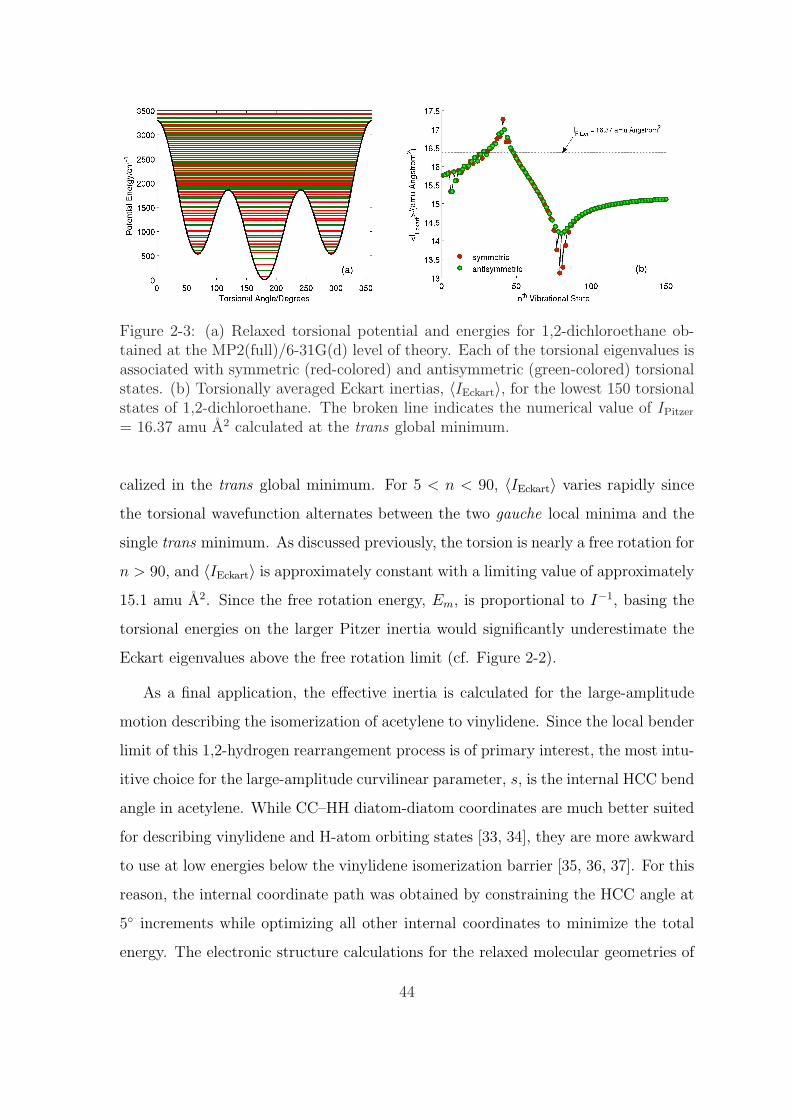
Figure 2-3: (a) Relaxed torsional potential and energies for 1,2-dichloroethane ob-tained at the MP2(full)/6-31G(d) level of theory. Each of the torsional eigenvalues isassociated with symmetric (red-colored) and antisymmetric (green-colored) torsionalstates. (b) Torsionally averaged Eckart inertias, 〈IEckart〉, for the lowest 150 torsionalstates of 1,2-dichloroethane. The broken line indicates the numerical value of IPitzer
= 16.37 amu A2 calculated at the trans global minimum.
calized in the trans global minimum. For 5 < n < 90, 〈IEckart〉 varies rapidly since
the torsional wavefunction alternates between the two gauche local minima and the
single trans minimum. As discussed previously, the torsion is nearly a free rotation for
n > 90, and 〈IEckart〉 is approximately constant with a limiting value of approximately
15.1 amu A2. Since the free rotation energy, Em, is proportional to I−1, basing the
torsional energies on the larger Pitzer inertia would significantly underestimate the
Eckart eigenvalues above the free rotation limit (cf. Figure 2-2).
As a final application, the effective inertia is calculated for the large-amplitude
motion describing the isomerization of acetylene to vinylidene. Since the local bender
limit of this 1,2-hydrogen rearrangement process is of primary interest, the most intu-
itive choice for the large-amplitude curvilinear parameter, s, is the internal HCC bend
angle in acetylene. While CC–HH diatom-diatom coordinates are much better suited
for describing vinylidene and H-atom orbiting states [33, 34], they are more awkward
to use at low energies below the vinylidene isomerization barrier [35, 36, 37]. For this
reason, the internal coordinate path was obtained by constraining the HCC angle at
5 increments while optimizing all other internal coordinates to minimize the total
energy. The electronic structure calculations for the relaxed molecular geometries of
44
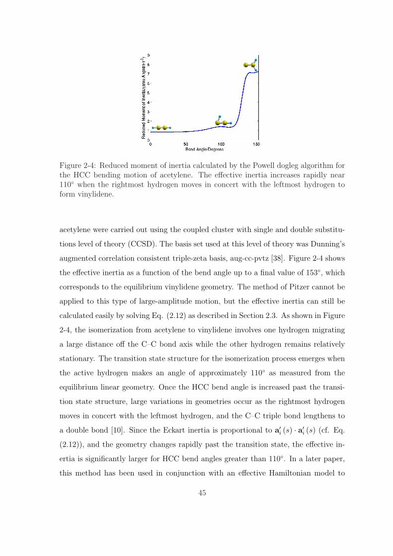
Figure 2-4: Reduced moment of inertia calculated by the Powell dogleg algorithm forthe HCC bending motion of acetylene. The effective inertia increases rapidly near110 when the rightmost hydrogen moves in concert with the leftmost hydrogen toform vinylidene.
acetylene were carried out using the coupled cluster with single and double substitu-
tions level of theory (CCSD). The basis set used at this level of theory was Dunning’s
augmented correlation consistent triple-zeta basis, aug-cc-pvtz [38]. Figure 2-4 shows
the effective inertia as a function of the bend angle up to a final value of 153, which
corresponds to the equilibrium vinylidene geometry. The method of Pitzer cannot be
applied to this type of large-amplitude motion, but the effective inertia can still be
calculated easily by solving Eq. (2.12) as described in Section 2.3. As shown in Figure
2-4, the isomerization from acetylene to vinylidene involves one hydrogen migrating
a large distance off the C–C bond axis while the other hydrogen remains relatively
stationary. The transition state structure for the isomerization process emerges when
the active hydrogen makes an angle of approximately 110 as measured from the
equilibrium linear geometry. Once the HCC bend angle is increased past the transi-
tion state structure, large variations in geometries occur as the rightmost hydrogen
moves in concert with the leftmost hydrogen, and the C–C triple bond lengthens to
a double bond [10]. Since the Eckart inertia is proportional to a′i (s) · a′i (s) (cf. Eq.
(2.12)), and the geometry changes rapidly past the transition state, the effective in-
ertia is significantly larger for HCC bend angles greater than 110. In a later paper,
this method has been used in conjunction with an effective Hamiltonian model to
45
describe the Stark effect as a diagnostic tool for assigning excited vibrational states
[10].
2.6 Conclusion
This chapter has presented a method by which accurate inertias for internal rotations
and other large-amplitude motions may be calculated by rigorously separating this
large-amplitude motion from the external rotation. It was shown that the conven-
tional Pitzer scheme for estimating the effective inertia can have large differences from
the Eckart method, which minimizes the couplings of torsions to rotations. The dis-
crepancies are mostly due to more accurate numerical minimization methods presently
available and are not meant to imply a criticism of Pitzer’s earlier work, whose ap-
proximate analytical formulae were pioneering at the time they were proposed. The
source of error in Pitzer’s inertia is apparent if one remembers that the Pitzer method
is inherently based on a coordinate system used from PAM. If the rotating top has
an axis of symmetry, the principal axes of the molecule do not change significantly as
the torsional angle is varied. However, if both the rotating top and the frame of the
molecule are heavy and asymmetric, the cross terms, which represent the interactions
between the two kinds of rotation (cf. Eq. (2.9)), are much larger in PAM/Pitzer’s
method than in the Eckart frame. In order to correct this inadequacy, it is neces-
sary to go beyond approximate analytical formulae to pursue numerical methods of
minimizing these couplings.
It was also shown that the Eckart method is general and applies to other large-
amplitude motions such as large variations in angle bends. In a one-dimensional
description of the acetylene/vinylidene isomerization, the procedure is essential since
it minimizes several of the coupling terms between the large-amplitude bend and
the overall rotation. This is particularly important since the relaxed geometries that
describe the 1,2-hydrogen rearrangement do not change uniformly along the isomer-
ization path. A user-friendly code for computing the Eckart inertia as a function of
the torsional angle is available [18]. These computer programs automatically solve
46

the nonlinear set of equations in Eq. (2.17) and output the reduced inertias as a
function of the torsional angle. All of the examples presented in Table 2.1 are also
available as sample inputs for these codes. The Eckart method described in Section
2.3 is recommended as an alternative to the conventional Pitzer method, particularly
for molecules with asymmetric internal rotors.
47

48

Chapter 3
Electronic Signatures of
Large-Amplitude Motion in S0
Acetylene
The primary objective of this chapter is to illustrate the use of electronic properties
to identify vibrationally excited states of S0 acetylene. The majority of the work in
this chapter resulted from a collaboration with Adam H. Steeves and was published
as an article in the Journal of Physical Chemistry B [10].
3.1 Introduction
The acetylene (H–C≡C–H) vinylidene (H2C=C:) isomerization on the ground elec-
tronic potential energy surface exemplifies one of the simplest bond-breaking processes
in polyatomic molecules. Numerous spectroscopic studies have been carried out on
acetylene [39, 40, 41, 42, 43], with the intent to observe the acetylene vinylidene
isomerization and to confirm theoretical calculations [33, 34, 35, 44, 45, 46, 47]. One
of the most recent studies on the spectroscopy of acetylene is that of Jacobson and
coworkers [39, 40, 48] who measured S1 → S0 dispersed fluorescence spectra, which
sample vibrational energy levels on the S0 surface in the energy region up to 15,000
cm−1. The excited vibrational states in this energy region lie close to the vinylidene
49
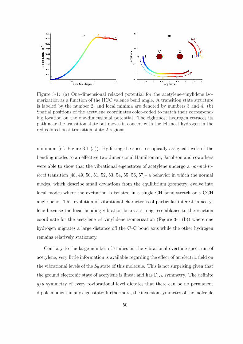
Figure 3-1: (a) One-dimensional relaxed potential for the acetylene-vinylidene iso-merization as a function of the HCC valence bend angle. A transition state structureis labeled by the number 2, and local minima are denoted by numbers 3 and 4. (b)Spatial positions of the acetylene coordinates color-coded to match their correspond-ing location on the one-dimensional potential. The rightmost hydrogen retraces itspath near the transition state but moves in concert with the leftmost hydrogen in thered-colored post transition state 2 regions.
minimum (cf. Figure 3-1 (a)). By fitting the spectroscopically assigned levels of the
bending modes to an effective two-dimensional Hamiltonian, Jacobson and coworkers
were able to show that the vibrational eigenstates of acetylene undergo a normal-to-
local transition [48, 49, 50, 51, 52, 53, 54, 55, 56, 57]– a behavior in which the normal
modes, which describe small deviations from the equilibrium geometry, evolve into
local modes where the excitation is isolated in a single CH bond-stretch or a CCH
angle-bend. This evolution of vibrational character is of particular interest in acety-
lene because the local bending vibration bears a strong resemblance to the reaction
coordinate for the acetylene vinylidene isomerization (Figure 3-1 (b)) where one
hydrogen migrates a large distance off the C–C bond axis while the other hydrogen
remains relatively stationary.
Contrary to the large number of studies on the vibrational overtone spectrum of
acetylene, very little information is available regarding the effect of an electric field on
the vibrational levels of the S0 state of this molecule. This is not surprising given that
the ground electronic state of acetylene is linear and has D∞h symmetry. The definite
g/u symmetry of every rovibrational level dictates that there can be no permanent
dipole moment in any eigenstate; furthermore, the inversion symmetry of the molecule
50

restricts the action of the dipole operator to off-diagonal in the vibrational quantum
numbers (see Section 3.4). That is, there is no permanent electric dipole moment
in acetylene that can lead to a pure rotational transition. Despite the absence of
a permanent vibrational dipole moment, Barnes et al. have analyzed electric field-
induced perturbations in ν1 + 3ν3 and ν2 + 3ν3 bands of acetylene at fields up to
300 kV/cm [58, 59]. In both cases, the primary effect of the electric field is to mix
the optically bright vibrational state with a near-degenerate optically dark level that
differs from the bright level by exchanging one quantum of excitation in the symmetric
C–H stretching mode (ν1, g) for one quantum of excitation in the antisymmetric C–H
stretching mode (ν3, u), or vice versa. The electric dipole moment function of S0
acetylene has also been studied by breaking the inversion symmetry through isotopic
substitution. Muenter and Laurie first observed the pure rotational transitions of
acetylene-d in the ground vibrational state [60]. Matsumura et al. subsequently
measured states excited in the CCH and CCD bending vibrations and determined
the variation of the dipole moment with excitation in these modes to be 0.046 and
-0.0336 D/quanta respectively [61].
In light of these spectroscopic and other theoretical results [62], it was proposed
that changes in electronic structure can be used as a universal marker to distinguish
the unique local mode vibrational states from the vast majority of normal vibra-
tional eigenstates. In any given energy region, the majority of vibrational states have
excitation energy distributed among many small-amplitude, strongly-coupled modes
[63]. Because the vibrational energy is distributed throughout the molecule, rather
than being directed along one particular large-amplitude coordinate, the average elec-
tronic structure does not significantly deviate from that of the equilibrium nuclear
configuration. However, for a large-amplitude, local motion, changes in the relative
orientations of functional groups in a molecule can cause large changes in the electric
dipole moment. The electronic wavefunction is even more severely deformed in the
case of chemical isomerization in which bonds are broken and new bonds formed,
thereby altering the global electronic structure. Therefore, the measured magnitude
of the electric dipole moment can be experimentally used as a measure of progress
51
along the reaction coordinate.
The following sections utilize the one-dimensional reaction path-like Hamilto-
nian developed in Chapter 2 to put the predictions of these dipole moments on
a quantitative basis. This reduced form of the full seven-dimensional vibrational
Hamiltonian is suitable for calculations of vibrationally averaged dipole moments of
both local stretching and local bending modes. Although multidimensional poten-
tial energy surfaces of acetylene can presently be calculated with excellent accuracy
[33, 34, 36, 64, 65], physical insight can be obtained from an effective, one-dimensional
ab initio calculation. The present approach to this enormous reduction in phase space
dimension is based on the observation that the spectroscopic fitting Hamiltonian, Heff,
exhibits extremely stable, one-dimensional, pure local bending motions. Therefore, a
Hamiltonian parametrized by a single internal coordinate is used in which the relevant
large-amplitude motion is decoupled from the other degrees of freedom. Numerical
comparisons with other models and experimental data allow the assessment of the
physical relevance of this reduction.
3.2 Hamiltonian
The theory of the internal coordinate path Hamiltonian and its variational solution
has been described by Tew et al. [12] Their parametrization of a large-amplitude
motion with a single internal coordinate is based on the work of Hougen, Bunker, and
Johns, who were the first workers to include large-amplitude motion in their semi-
rigid bender model [8]. Other workers, such as Szalay, have extended this approach to
account for non-rigid effects of large-amplitude internal motion in general molecules
[66]. The formulation of Tew et al. is closely related to the reaction path Hamiltonian
introduced by Miller, Handy, and Adams [13] with the exception that the internal
coordinate path need not be exactly parallel to the minimum energy path. When
defining a path to parametrize a large-amplitude motion, it should be remembered
that the minimum energy path is defined as the steepest descent path from a transition
state toward reactants or products [67, 68]. More rigorously, the minimum energy
52
path can be expressed by the solution of the differential equation
dx
ds= − ∇V
|∇V | , (3.1)
where x is a 3N component vector of mass-weighted Cartesian coordinates, s is the
path length, and V is the potential energy of N nuclear displacement vectors. When
the minimum energy path is located in mass-weighted coordinates as written in Eq.
(3.1), it is called an intrinsic reaction coordinate [67, 68]. Since the minimum energy
path by definition follows the gradient vector of the potential energy, the potential
energy at any point on the path can be expanded in terms of the normal coordinates
Qk up to second order:
V = V0 (s) + 12
3N−7∑
k=1
ω2k (s) Q2
k, (3.2)
where ω2k (s) are the 3N − 7 eigenvalues of a projected force constant matrix.
In order to define a minimum energy path, one commences by optimizing a saddle
point on the potential energy surface and then follows the negative gradient of the
energy in mass-weighted Cartesian coordinates. However, as Tew et al. have stated,
this algorithm is not a numerically sound technique. If insufficiently small steps are
taken along the reaction path, one may be unable to locate the minimum accurately
at the end of the path. Furthermore, near the saddle point, the optimized geometries
may be inaccurate since the first step away from this starting point is along a vector
defined without reference to any curvature. The internal coordinate path Hamiltonian
used in this work removes many of these problems by parametrizing a path with
a single internal coordinate such as a bond length or a valence bend angle. This
parametrization guarantees a continuous variation with no numerical complexity since
the internal coordinate is a geometric variable and is always well-defined at any point
on the path. However, since this path is obtained by scanning relaxed points on the
potential surface with a user-chosen internal coordinate, the gradient vector of the
molecular potential energy has not necessarily been followed. Whereas the minimum
energy path potential energy has no term linear in Qk, the internal coordinate path
53

potential must have a linear term:
V = V0 (s) +3N−7∑
k=1
gk (s) Qk + 12
3N−7∑
k=1
ω2k (s) Q2
k, (3.3)
where s is a conveniently chosen geometric variable such as an angle, a bond length,
or a combination of angles and bond lengths used to parametrize the large-amplitude
path. For many cases, the true reaction coordinate can be approximated by a single
internal coordinate, and the gradient gk will be small if the internal coordinate is
approximately in the same direction as s. In other words, neglecting this gradient
term is equivalent to ignoring the minor off-diagonal matrix elements of gk (s) Qk in
the small-amplitude harmonic quantum numbers.
In the present work the internal coordinate path method is used with an ap-
proximate treatment for the other small-amplitude modes. The approximate ex-
pressions and their numerical evaluations have already been reported in Chapter
2. This approach is briefly reviewed here, and only the slight modifications used
in the present work will be described in detail. The theory of the internal coor-
dinate path Hamiltonian for an N -atom molecule is expressed in terms of a single
large-amplitude coordinate, s , its conjugate momentum, ps (= −i~∂/∂s), and the
coordinates Q = Q1, Q2, . . . , Q3N−7 and momenta P =
P1, P2, . . . , P3N−7
=
−i~ ∂/∂Q1, ∂/∂Q2, . . . , ∂/∂Q3N−7 of the orthogonal small-amplitude vibrational
modes. The full quantum mechanical kinetic energy operator in these coordinates
is given by
T = 12
4∑
d,e=1
µ1/4(Πd − πd
)µdeµ
−1/2(Πe − πe
)µ1/4 + 1
2
3N−7∑
k=1
µ1/4Pkµ−1/2Pkµ
1/4. (3.4)
Π and π are four-component operators given by
Π =(Jx, Jy, Jz, ps
),
π =3N−7∑
k,l=1
(Bkl,x (s) , Bkl,y (s) , Bkl,z (s) , Bkl,s (s)) QkPl,(3.5)
54
where Jx, Jy, and Jz are the components of the total angular momentum operator,
and Bkl,x, Bkl,y, Bkl,z, and Bkl,s are the “Coriolis coupling” matrices [12] that are
functions of the large-amplitude coordinate, s. The symmetric tensor, µde, and its
determinant, µ, are also functions of the internal coordinate, s.
As reported previously [7], the following approximations allow for the computation
to be manageable: (1) the effective inertia tensor depends weakly on Q, and only the
terms that depend on s are retained; (2) the “vibrational angular momentum” terms,
πα, are linear in the small-amplitude coordinates, Q, and their contribution to the
kinetic energy is neglected; (3) numerically enforcing the Eckart conditions minimizes
many of the coupling terms in Eq. (3.1). It follows from these approximations that
the kinetic energy operator for total angular momentum J = 0 can be written in the
following form (cf. Eq. 10 of Ref. [7]):
T = 12psI
−10ssps + 1
2µ1/4
(psI
−10ssµ
−1/2(psµ
1/4))
+ 12
3N−7∑
k=1
P 2k , (3.6)
where the scalar terms I−10ss and µ are given by
I−10ss (s) =
(N∑
i=1
a′i (s) · a′i (s))−1
, (3.7)
µ (s) = I−10ss · det
(I−10
). (3.8)
The vectors ai
(= m
1/2i ri
)are the mass-weighted Cartesian coordinates of the ith
atom at a point on the path s with respect to the Eckart axis system, and a′i = dai/ds.
Finally, the operator ps operates only within the parentheses in Eq. (3.6); that is,
the next to last term in Eq. (3.6) is a scalar term.
3.3 Ab Initio Calculations
All ab initio electronic structure calculations for the acetylene-vinylidene isomeriza-
tion were carried out with the Gaussian 03 package [25]. Extensive theoretical studies
55
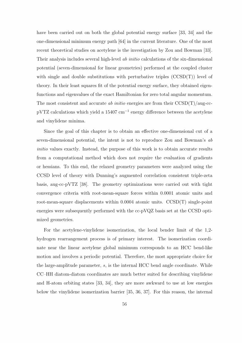
have been carried out on both the global potential energy surface [33, 34] and the
one-dimensional minimum energy path [64] in the current literature. One of the most
recent theoretical studies on acetylene is the investigation by Zou and Bowman [33].
Their analysis includes several high-level ab initio calculations of the six-dimensional
potential (seven-dimensional for linear geometries) performed at the coupled cluster
with single and double substitutions with perturbative triples (CCSD(T)) level of
theory. In their least squares fit of the potential energy surface, they obtained eigen-
functions and eigenvalues of the exact Hamiltonian for zero total angular momentum.
The most consistent and accurate ab initio energies are from their CCSD(T)/aug-cc-
pVTZ calculations which yield a 15407 cm−1 energy difference between the acetylene
and vinylidene minima.
Since the goal of this chapter is to obtain an effective one-dimensional cut of a
seven-dimensional potential, the intent is not to reproduce Zou and Bowman’s ab
initio values exactly. Instead, the purpose of this work is to obtain accurate results
from a computational method which does not require the evaluation of gradients
or hessians. To this end, the relaxed geometry parameters were analyzed using the
CCSD level of theory with Dunning’s augmented correlation consistent triple-zeta
basis, aug-cc-pVTZ [38]. The geometry optimizations were carried out with tight
convergence criteria with root-mean-square forces within 0.0001 atomic units and
root-mean-square displacements within 0.0004 atomic units. CCSD(T) single-point
energies were subsequently performed with the cc-pVQZ basis set at the CCSD opti-
mized geometries.
For the acetylene-vinylidene isomerization, the local bender limit of the 1,2-
hydrogen rearrangement process is of primary interest. The isomerization coordi-
nate near the linear acetylene global minimum corresponds to an HCC bend-like
motion and involves a periodic potential. Therefore, the most appropriate choice for
the large-amplitude parameter, s, is the internal HCC bend angle coordinate. While
CC–HH diatom-diatom coordinates are much better suited for describing vinylidene
and H-atom orbiting states [33, 34], they are more awkward to use at low energies
below the vinylidene isomerization barrier [35, 36, 37]. For this reason, the internal
56
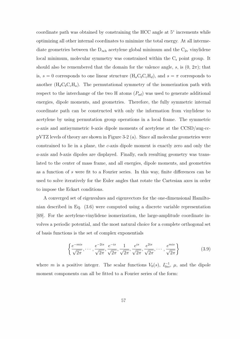
coordinate path was obtained by constraining the HCC angle at 5 increments while
optimizing all other internal coordinates to minimize the total energy. At all interme-
diate geometries between the D∞h acetylene global minimum and the C2v vinylidene
local minimum, molecular symmetry was constrained within the Cs point group. It
should also be remembered that the domain for the valence angle, s, is (0, 2π); that
is, s = 0 corresponds to one linear structure (HaCbCcHd), and s = π corresponds to
another (HdCbCcHa). The permutational symmetry of the isomerization path with
respect to the interchange of the two H atoms (Pad) was used to generate additional
energies, dipole moments, and geometries. Therefore, the fully symmetric internal
coordinate path can be constructed with only the information from vinylidene to
acetylene by using permutation group operations in a local frame. The symmetric
a-axis and antisymmetric b-axis dipole moments of acetylene at the CCSD/aug-cc-
pVTZ levels of theory are shown in Figure 3-2 (a). Since all molecular geometries were
constrained to lie in a plane, the c-axis dipole moment is exactly zero and only the
a-axis and b-axis dipoles are displayed. Finally, each resulting geometry was trans-
lated to the center of mass frame, and all energies, dipole moments, and geometries
as a function of s were fit to a Fourier series. In this way, finite differences can be
used to solve iteratively for the Euler angles that rotate the Cartesian axes in order
to impose the Eckart conditions.
A converged set of eigenvalues and eigenvectors for the one-dimensional Hamilto-
nian described in Eq. (3.6) were computed using a discrete variable representation
[69]. For the acetylene-vinylidene isomerization, the large-amplitude coordinate in-
volves a periodic potential, and the most natural choice for a complete orthogonal set
of basis functions is the set of complex exponentials
e−mis
√2π
, · · · ,e−2is
√2π
,e−is
√2π
,1√2π
,eis
√2π
,e2is
√2π
, · · · ,emis
√2π
(3.9)
where m is a positive integer. The scalar functions V0(s), I−10ss, µ, and the dipole
moment components can all be fitted to a Fourier series of the form:
57

Figure 3-2: Dipole moments computed for relaxed geometries as a function of (a)fixed HCC local bend angle and (b) fixed local C–H stretch distance. In Figure 3-2(a), the schematic diagrams of the bending motion show that when the local bend isexcited, the b-axis dipole moment must change sign at θ = 0. Conversely, the a-axisdipole moment is symmetric about θ = 0 since the active hydrogen is always placed atidentical horizontal distances along the a-axis during the (symmetric) local bendingmotion. In Figure 3-2 (b), the broken line indicates the numerical value of the dipolemoment for the CCH equilibrium geometry. The dipole moments for Figures 3-2 (a)and (b) were obtained from the CCSD/aug-cc-pVTZ and MR-AQCC/aug-cc-pVQZlevels of theory, respectively.
f (s) =a0
2+
[(N−1)/2]∑j=1
aj cos (js) +
[(N−1)/2]∑j=1
bj sin (js), (3.10)
where N is the number of discrete data points to be fitted, and the square brackets
[(N − 1)/2], denote the largest integer less than or equal to (N − 1)/2. The nonvan-
ishing matrix elements of Eq. (3.10), Fk,k′ = 〈k| f (s) |k′〉, in the ordered basis listed
in Eq. (3.9) are
Fk,k =a0
2,
Fk,k+l =al + ibl
2,
Fk+l,k = F ∗k,k+l =
al − ibl
2,
(3.11)
Since the maximum value of l is max (j) = [(N − 1) /2], the structure of F is an
N -diagonal, (2m + 1)× (2m + 1) Hermitian matrix. The matrix representation of ps
is a (2m + 1)× (2m + 1) diagonal matrix with [−m~, · · · ,−2~,−~, 0, ~, 2~, · · · ,m~]
along the diagonal. Using Eqs. (3.10) and (3.11) the kinetic energy, potential energy,
58
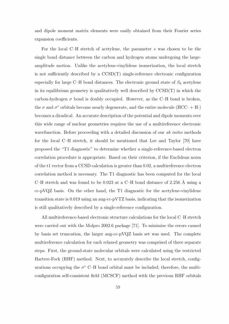
and dipole moment matrix elements were easily obtained from their Fourier series
expansion coefficients.
For the local C–H stretch of acetylene, the parameter s was chosen to be the
single bond distance between the carbon and hydrogen atoms undergoing the large-
amplitude motion. Unlike the acetylene-vinylidene isomerization, the local stretch
is not sufficiently described by a CCSD(T) single-reference electronic configuration
especially for large C–H bond distances. The electronic ground state of S0 acetylene
in its equilibrium geometry is qualitatively well described by CCSD(T) in which the
carbon-hydrogen σ bond is doubly occupied. However, as the C–H bond is broken,
the σ and σ∗ orbitals become nearly degenerate, and the entire molecule (HCC· + H·)becomes a diradical. An accurate description of the potential and dipole moments over
this wide range of nuclear geometries requires the use of a multireference electronic
wavefunction. Before proceeding with a detailed discussion of our ab initio methods
for the local C–H stretch, it should be mentioned that Lee and Taylor [70] have
proposed the “T1 diagnostic” to determine whether a single-reference-based electron
correlation procedure is appropriate. Based on their criterion, if the Euclidean norm
of the t1 vector from a CCSD calculation is greater than 0.02, a multireference electron
correlation method is necessary. The T1 diagnostic has been computed for the local
C–H stretch and was found to be 0.023 at a C–H bond distance of 2.256 A using a
cc-pVQZ basis. On the other hand, the T1 diagnostic for the acetylene-vinylidene
transition state is 0.019 using an aug-cc-pVTZ basis, indicating that the isomerization
is still qualitatively described by a single-reference configuration.
All multireference-based electronic structure calculations for the local C–H stretch
were carried out with the Molpro 2002.6 package [71]. To minimize the errors caused
by basis set truncation, the larger aug-cc-pVQZ basis set was used. The complete
multireference calculation for each relaxed geometry was comprised of three separate
steps. First, the ground-state molecular orbitals were calculated using the restricted
Hartree-Fock (RHF) method. Next, to accurately describe the local stretch, config-
urations occupying the σ∗ C–H bond orbital must be included; therefore, the multi-
configuration self-consistent field (MCSCF) method with the previous RHF orbitals
59
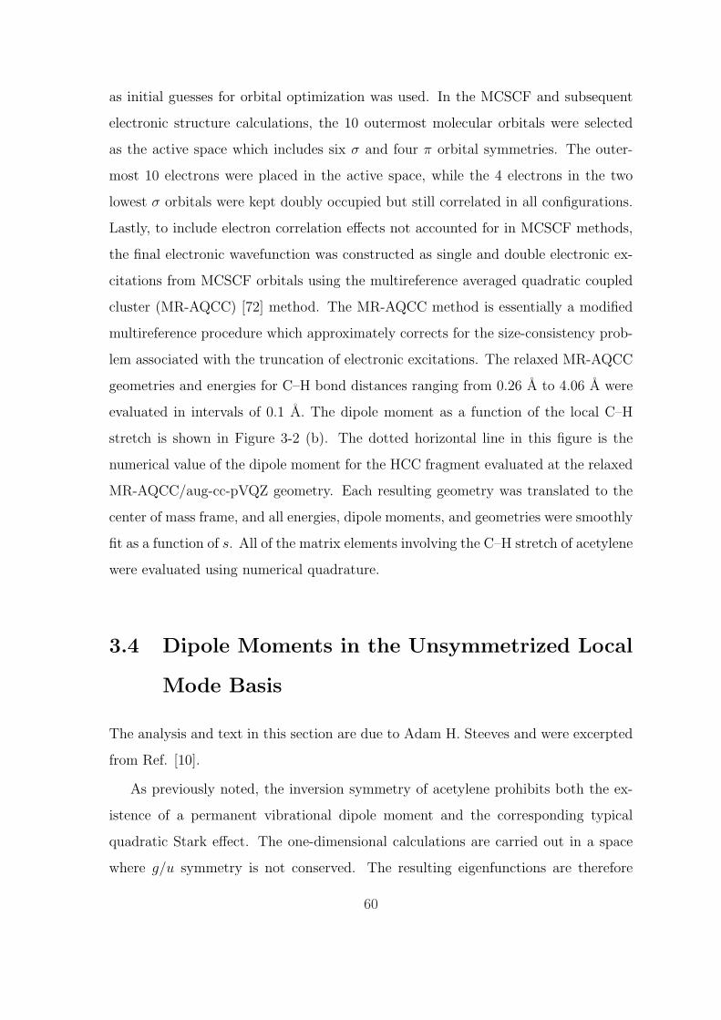
as initial guesses for orbital optimization was used. In the MCSCF and subsequent
electronic structure calculations, the 10 outermost molecular orbitals were selected
as the active space which includes six σ and four π orbital symmetries. The outer-
most 10 electrons were placed in the active space, while the 4 electrons in the two
lowest σ orbitals were kept doubly occupied but still correlated in all configurations.
Lastly, to include electron correlation effects not accounted for in MCSCF methods,
the final electronic wavefunction was constructed as single and double electronic ex-
citations from MCSCF orbitals using the multireference averaged quadratic coupled
cluster (MR-AQCC) [72] method. The MR-AQCC method is essentially a modified
multireference procedure which approximately corrects for the size-consistency prob-
lem associated with the truncation of electronic excitations. The relaxed MR-AQCC
geometries and energies for C–H bond distances ranging from 0.26 A to 4.06 A were
evaluated in intervals of 0.1 A. The dipole moment as a function of the local C–H
stretch is shown in Figure 3-2 (b). The dotted horizontal line in this figure is the
numerical value of the dipole moment for the HCC fragment evaluated at the relaxed
MR-AQCC/aug-cc-pVQZ geometry. Each resulting geometry was translated to the
center of mass frame, and all energies, dipole moments, and geometries were smoothly
fit as a function of s. All of the matrix elements involving the C–H stretch of acetylene
were evaluated using numerical quadrature.
3.4 Dipole Moments in the Unsymmetrized Local
Mode Basis
The analysis and text in this section are due to Adam H. Steeves and were excerpted
from Ref. [10].
As previously noted, the inversion symmetry of acetylene prohibits both the ex-
istence of a permanent vibrational dipole moment and the corresponding typical
quadratic Stark effect. The one-dimensional calculations are carried out in a space
where g/u symmetry is not conserved. The resulting eigenfunctions are therefore
60

not eigenfunctions of the inversion operator and may possess permanent vibrational
dipole moments. In order to make the comparison with experiment, one must consider
the local-mode interpretation of the electric field induced perturbation investigated
by Barnes et al. and demonstrate how the local mode limit of vibrational character
leads to an effective dipole of the g/u components.
The matrix element connecting the optically bright and dark field-free eigenstates
is an off-diagonal (in vibration) element of the electric dipole operator, or a transition
dipole moment, 〈04+|µ |04−〉. The local mode notation can be expressed in terms of
the left and right oscillators,
|04±〉 =1√2
[|04〉 ± |40〉] , (3.12)
where the notation on the right hand side of Eq. (3.12) indicates an unsymmetrized
basis state |υleftυright〉. The dipole matrix element can be re-expressed in the unsym-
metrized basis as:
〈04+|µ |04−〉 =1
2[〈04|µ |04〉 − 〈40|µ |40〉] . (3.13)
Since, by symmetry, the two diagonal elements of the dipole operator in the unsym-
metrized basis are of the same magnitude but of opposite sign,
〈04|µ |04〉 = −〈40|µ |40〉 , (3.14)
the perturbation matrix element in the symmetrized basis can be expressed as a
diagonal matrix element in the left/right basis:
〈04+|µ |04−〉 = 〈04|µ |04〉 . (3.15)
The transition dipole moment between the vibrational levels that make up the lo-
cal mode pair can therefore be interpreted as a permanent vibrational dipole moment
of an unsymmetrized state excited only in the right (or left) oscillator. Because the
61

+/- (g/u) components have been brought into near degeneracy, each rovibrational
level now interacts with the rotational levels differing in J by one that belong to the
other member of the local mode pair, through the dipole operator. The inversion
symmetry has therefore been effectively broken because the physical consequences of
the near degeneracy in the local mode limit are essentially identical to breaking the
symmetry of the molecule through other means, e.g. isotopic substitution. That is,
when the molecule is excited to a vibrational level that is in the local mode limit,
it will exhibit regular quadratic Stark shifts, and it will be possible to excite “pure
rotational” transitions.
3.5 Local Bending in the Polyad Model
The polyad model is a multi-resonant effective Hamiltonian fitted to an extensive set
of spectroscopic data [48, 73, 74, 75, 76]. Although the local bending levels are not
directly observed by any of the spectroscopic techniques and therefore not included
in the fit, they emerge naturally from the effective Hamiltonian model. The local
mode basis for bending levels is more complicated than that for the stretching levels
because each CCH oscillator is treated as an isotropic two-dimensional harmonic
oscillator and therefore is characterized by a vibrational angular momentum. In the
symmetrized local mode basis, a state is labeled∣∣∣υ`A
A , υ`BB
⟩g/u±
L, where `A/B refers
to the vibrational angular momenta associated with the left or right local bending
mode. While the extreme local bender levels are denoted |N0bend, 0
0〉g/u±L , the higher
lying levels are formed by removing one quantum of vibration from the highly excited
oscillator and placing it in the less excited oscillator, e.g.∣∣(Nbend − 1)1 , 1−1
⟩g/u±L ,
∣∣(Nbend − 2)0 , 20⟩g/u±L , etc.
3.6 Results
The local-bending behavior that emerges from the polyad model represents a reduc-
tion to one dimension of the full spectroscopic effective Hamiltonian. The spectro-
62

scopic fitting Hamiltonian itself is dimensionally reduced from 7 to 3 by the speci-
fication of Nstretch, Nbend, `, and g/u symmetry (7 – 1 (Nstretch) – 1 (Nres = Nbend)
– 1 (` = 0) – 1 (g/u) = 3). Similarly, the internal coordinate path treatment of
the vibrational level structure reduces the ab initio potential energy surface to one
dimension.
The agreement between the frequencies calculated from the one-dimensional ab
initio model and the experimentally determined effective Hamiltonian model is gen-
erally good (< 20 cm−1) in the region where the local-bender is believed to be an
accurate description of the lowest members of each polyad (Figure 3-3). For the pur-
pose of comparison with the one-dimensional calculations, the frequency of the local
bending vibration was determined from the polyad model by calculating the energy
difference between the lowest members of successive gerade pure-bending polyads with
even values of Nbend, 0+g and dividing by two. Near 18 quanta of Nbend, the frequen-
cies calculated from the polyad model and those calculated from the one-dimensional
cut through an ab initio potential pass through each other. The close match between
the vibrational frequencies supports the assertion that both models describe the same
class of essentially one-dimensional large-amplitude motion. This agreement is par-
ticularly notable since the two calculations arise from drastic reductions in dimension
of two very different (empirical vs. ab initio) Hamiltonians.
As anticipated from knowledge of the evolution of the vibrational character,
the agreement between the two Hamiltonians occurs over a limited range. Below
Nbend = 10, the disagreement between the two models reaches 50 cm−1, which is
not surprising because the lowest members of the pure-bending polyads are well-
described in the normal mode rather than the local mode basis. Above 22 quanta of
local bending, the ab initio frequency decreases rapidly, to values below 600 cm−1,
as the bending vibration starts to sample the barrier to isomerization (by tunneling
through this barrier), and the approximately stationary hydrogen abruptly starts to
migrate off axis to its vinylidene position. This behavior is not captured by the polyad
model (because there is nothing barrier-related in the spectroscopic Heff), in which
the vibrational frequency continues to decrease at a relatively constant rate.
63
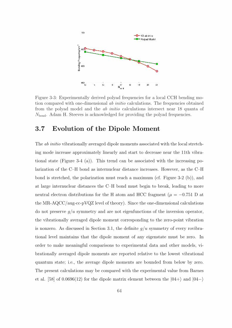
Figure 3-3: Experimentally derived polyad frequencies for a local CCH bending mo-tion compared with one-dimensional ab initio calculations. The frequencies obtainedfrom the polyad model and the ab initio calculations intersect near 18 quanta ofNbend. Adam H. Steeves is acknowledged for providing the polyad frequencies.
3.7 Evolution of the Dipole Moment
The ab initio vibrationally averaged dipole moments associated with the local stretch-
ing mode increase approximately linearly and start to decrease near the 11th vibra-
tional state (Figure 3-4 (a)). This trend can be associated with the increasing po-
larization of the C–H bond as internuclear distance increases. However, as the C–H
bond is stretched, the polarization must reach a maximum (cf. Figure 3-2 (b)), and
at large internuclear distances the C–H bond must begin to break, leading to more
neutral electron distributions for the H atom and HCC fragment (µ = −0.751 D at
the MR-AQCC/aug-cc-pVQZ level of theory). Since the one-dimensional calculations
do not preserve g/u symmetry and are not eigenfunctions of the inversion operator,
the vibrationally averaged dipole moment corresponding to the zero-point vibration
is nonzero. As discussed in Section 3.1, the definite g/u symmetry of every rovibra-
tional level maintains that the dipole moment of any eigenstate must be zero. In
order to make meaningful comparisons to experimental data and other models, vi-
brationally averaged dipole moments are reported relative to the lowest vibrational
quantum state; i.e., the average dipole moments are bounded from below by zero.
The present calculations may be compared with the experimental value from Barnes
et al. [58] of 0.0696(12) for the dipole matrix element between the |04+〉 and |04−〉
64

Figure 3-4: Vibrationally averaged ab initio dipole moments computed (a) for a localC–H stretch and (b) for a local bend. Since the b-axis dipole moment for the local bendis antisymmetric with respect to the equilibrium bend angle, its vibrational average isexactly zero, and only the vibrational average for the a-axis dipole is displayed. Thebottom axis of Figure 3-4 (b) is numbered according to the vibrational level in thefully permutational symmetric isomerization path, and the top axis labels only thesymmetric vibrational levels. Both averaged dipole moments are reported relative tothe lowest vibrational quantum state.
local mode stretching states. The calculated value of 0.0966 D is quite reasonable
for the one-dimensional model. Some of this discrepancy is due to the fact that the
acetylene stretching system, at this level of excitation, is in the intermediate case
between the pure normal and pure local mode limits [52]. Experimental evidence
that the local mode limit has not been reached is provided by the non-zero difference
in vibrational excitation energies between the g and u states. The difference in ener-
gies has been measured to be 4.133(16) cm−1. The one-dimensional model will only
apply to the pure local mode limit, while excitation of the other C–H bond oscillator
must lead to a partial cancellation of the dipole due to its large-amplitude motion.
The experimental value embodies this partial cancellation, while the one-dimensional
model does not.
Figure 3-4 (b) shows the vibrationally averaged dipole moments for the full per-
mutationally symmetric isomerization path with respect to the interchange of the
two H atoms. The bottom axis of Figure 3-4 (b) is numbered according to the vi-
brational quantum numbers in this symmetric HaCbCcHd HdCbCcHa double-well
potential. Because of this symmetry, the lowest average dipole moments come in
pairs corresponding to nuclear permutational splittings between symmetric and anti-
65

symmetric vibrational states. Throughout this chapter the numbering scheme at the
top axis of Figure 3-4 (b) is used in which only the symmetric vibrational states in
the one-dimensional bending model are labeled. It can be seen that the vibrationally
averaged dipole moments obey a nearly linear trend up to 22 quanta of vibrational
excitation, increasing approximately 0.053 D per quantum of excitation (the slope
was determined using a least squares method on the lowest 10 data points). As in
the case of the C–H stretching, the calculated value overestimates the value available
from experiment. The value of the slope obtained from the relatively low energy ex-
cited states of acetylene-d by Matsumura et al. [61], 0.046 D is, in a manner similar
to that of the C–H stretching modes, not reflective of the pure CCH bending motion.
Examination of the normal mode eigenvectors, obtained from an FG matrix analysis
based on the force constants of Strey and Mills [77], reveals that significant CCD
bending motion occurs in the nominally CCH bending mode, ν5. The calculated
dipole moment variation, in the linear region, is qualitatively due to the diminishing
projection of the C–H bond dipole on the C–C bond axis, leading to an imbalance
of the bond dipoles of the two C–H fragments. In the same energy region where the
vibrational frequency begins to decrease rapidly, the dipole moment increases more
quickly due to increased sampling of the isomerization barrier (3.33 D) and mixing
with the vinylidene configuration (2.35 D).
The υ = 25 excited vibrational level identified in the calculation clearly deviates
from the smooth linear trend of the lower-lying states. This level is associated with
the zero-point level of S0 vinylidene. Near the υ = 25 vibrational level, the averaged
dipole moments begin to change abruptly since the vibrational wavefunction begins
to sample both the acetylene and vinylidene minima. Above this energy, the dipole
moment oscillates between acetylene-localized states and values more typical of the
isomerization transition state before approaching a constant value of 2.0 D at high
local excitation.
66

3.8 Assignment of Large-Amplitude Local Bender
States
The analysis and text in this section are due to Adam H. Steeves and were excerpted
from Ref. [10].
Although the extreme local bender levels have been the primary focus of this
chapter, those that lie at the bottom of each pure-bending polyad, it is important
to note that the other members of pure-bending polyads can be described in the
local mode basis. Examination of the eigenfunctions obtained from the polyad model
reveals a transition at approximately 14 quanta of bending vibration, at which point
the lowest member of each pure-bending polyad is best described by a local CCH
bending motion [48]. This qualitative change in vibrational character is accompanied
by a decreasing energy difference between the lowest members of the 0+g and 0+
u
polyads. At Nbend = 10, this energy difference is > 10 cm−1, but it rapidly decreases
to < 10−3 cm−1 by Nbend = 14, and < 10−7 cm−1 by Nbend = 22. In Table 3.1
(a)–(c) the energy splittings between the lowest members of the g+ and u+ polyads
are compared for Nbend = 14 − 26. These lowest extreme local bender levels form
a local mode pair, and the transition dipole that couples them can be viewed as a
permanent vibrational dipole moment, as in the case of the acetylene C–H stretching
levels discussed in Section 3.7.
The ability to equate the one-dimensional calculation of the dipole moment with
the dipole created by imbalance in excitation of oscillators can be used for other
predictions. It enables the assignment of dipole moments to any basis state in the
local mode limit and therefore allows the calculation of the dipole moment for each
eigenstate based on the eigenvectors in the local mode basis. Predictions of the
dipole moments for the three lowest energy eigenstates of the Nbend = 14 − 26
polyads are found in Table 3.1 (a)–(c). Predictions are made in the same man-
ner as for the stretching case by neglecting the vibrational angular momentum, i.e.
µ (|142, 2−2〉L) = µ (|140, 20〉L). These lowest eigenstates are assigned to the local
mode states as |N0bend, 0
0〉g+L ,
∣∣(Nbend − 1)1 , 1−1⟩g+
L , and∣∣(Nbend − 2)0 , 20
⟩g+
L respec-
67

Nbend E(|N0
bend, 00〉g+L
)E(g+)− E(u+) µ (D)
14 8972.1 −1× 10⁻⁴ 0.8516 10236.9 −3× 10⁻⁵ 1.0218 11485.0 −4× 10⁻⁶ 1.2020 12717.4 −4× 10⁻⁷ 1.3622 13934.9 −4× 10⁻⁸ 1.5524 15137.9 −1× 10⁻⁹ 1.7726 16327.1 3× 10⁻¹⁰ 2.28
Nbend E(∣∣(Nbend − 1)1 , 1−1
⟩g+
L
)E(g+)− E(u+) µ (D)
14 9070.0∗ −9 —16 10352.4∗ −4× 10⁻² —18 11605.7 6× 10⁻⁵ 1.0120 12844.8 7× 10⁻⁵ 1.1822 14070.2 8× 10⁻⁶ 1.3624 15289.9 3× 10⁻⁷ 1.5426 16480.1 −8× 10⁻⁸ 1.76
Nbend E(∣∣(Nbend − 2)0 , 20
⟩g+
L
)E(g+)− E(u+) µ (D)
14 9037.0∗ −4× 10⁻² —16 10315.6 3× 10⁻³ 0.7818 11574.7 2× 10⁻⁴ 0.9320 12815.7 −8× 10⁻⁶ 1.0722 14040.2 −2× 10⁻⁶ 1.2024 15249.3 −1× 10⁻⁷ 1.3926 16443.9 1× 10⁻⁸ 1.54
Table 3.1: (a)–(c): Energy splittings between lowest members of the g+ and u+polyads and calculated dipole moments for Nbend = 14− 26. All energies and energydifferences reported are in units of cm−1. Energies denoted by an asterisk are notwell-described in the local mode basis using the Hose-Taylor criterion. The increasein dipole moment is accompanied by decreasing energy differences between the g+and u+ polyads. Adam H. Steeves is acknowledged for preparing this table.
68

tively, although only the lowest energy state in the Nbend = 14 polyad can be as-
signed based on the Hose-Taylor criterion [78]. As one moves towards the center
of each polyad, the local mode model describes each eigenstate less well. That is,
the eigenstates contain larger contributions from several local mode basis states, in-
cluding those with smaller differences in excitation between the two oscillators. This
trend causes the dipole moment to decrease faster than linearly inside a given polyad,
although at high excitation (Nbend ∼ 22) all of the listed states are described well by
the local mode basis.
The shape of the a-axis dipole moment function strongly resembles that of the
potential energy surface. The maximum value of the a-axis dipole is reached near
the transition state of the isomerization reaction, before the approximately station-
ary hydrogen begins to move off axis to form vinylidene. The near transition state
configuration represents the largest distortion of the electronic wavefunction. This is
ideal for performing high-resolution experiments because the larger dipole moments
are more readily observable via laser Stark spectroscopy. Even more useful is the
ability to identify particular vibrational levels based on the predictions of variation in
electronic structure. While electronic signatures of only two one-dimensional motions
have been described, vibrational states that do not consist of these special motions
are expected to be highly dynamically mixed. The ergodic nature of the highly mixed
vibrational levels imply that they will remain essentially silent to Stark effect mea-
surements, except in the case of accidental near degeneracies. The large-amplitude
states will be the only states with significant, regular Stark activity.
In addition, the dipole moments will help assign members of the |Nbend, 0〉g/u±L ,
|Nbend − 1, 1〉g/u±L , |Nbend − 2, 2〉g/u±
L , etc. family of states. This information is essen-
tial because once the energies of such assigned states are obtained from spectra, the
one-dimensional local mode potential can be experimentally refined. The relative en-
ergies of the|Nbend, 0〉g/u±
L , |Nbend − 1, 1〉g/u±L , |Nbend − 2, 2〉g/u±
L
and|Nbend + 1, 0〉g/u±
L |Nbend, 1〉g/u±L , |Nbend − 1, 2〉g/u±
L
etc. groups of local mode states,
supplemented by measured dipole moments, provide direct experimental characteri-
zation of the reaction coordinate near the barrier maximum.
69

3.9 Conclusions
A one-dimensional reduction of the full seven-dimensional ab initio S0 potential en-
ergy surface of C2H2 was explored, and it was found that it strongly resembles the
one-dimensional, local bending reduction of the empirical spectroscopic pure-bend ef-
fective Hamiltonian. These reductions in dimension occur when the large-amplitude
motion decouples from the other nuclear motions as a result of anharmonic detun-
ing from resonance. A comparison between the computed frequencies of the one-
dimensional ab initio potential and those of the spectroscopic effective Hamiltonian,
the parameters of which are refined against experimental data, exhibits good agree-
ment for the local bending motion. The results of Section 3.6 strongly indicate reduc-
tion of both ab initio and spectroscopic Hamiltonians to the same one-dimensional
potential even though the two Hamiltonians are derived from completely different
formalisms. This is particularly noteworthy since the spectroscopic effective Hamil-
tonian does not explicitly specify the displacement coordinates of the stable, one-
dimensional, localized, motion, but this one-dimensional path is explicitly defined
in the reaction path Hamiltonian. More importantly, the large-amplitude local vi-
brations which lead to changes in the electronic properties of acetylene, permits a
transition dipole between the two nearly degenerate g/u eigenstates associated with
the local mode. This near-degeneracy of the local mode pair, which indicates that the
g/u symmetry is ready to be broken, is a hallmark of local mode behavior. The large
changes in dipole moments along the local bending coordinate provide a method to
identify particular vibrational levels via the Stark effect. The dipole moment values
computed from the ab initio one-dimensional potential will be useful in distinguishing
extreme local mode states from the vastly more strongly mixed isoenergetic states.
70
Chapter 4
The Hyperfine Structure of HCN
and HNC
This chapter describes ongoing work pertaining to the nuclear quadrupole hyperfine
structures of HCN, HNC, and their isotopomers. The majority of the work in this
chapter resulted from a collaboration with Dr. Hans A. Bechtel.
4.1 Introduction
Similar to the acetylene vinylidene system described in Chapter 3, the primary
objective for studying the HCN HNC isomerization is to observe vibrational states
proximal to a barrier maximum. These highly excited vibrational states have am-
plitude localized along the minimum energy isomerization path and therefore reveal
features of the potential energy surface that control intramolecular dynamics. As
in the acetylene vinylidene isomerization, the magnitude of the electric dipole
moment is also an effective diagnostic for identifying delocalized states between the
HCN and HNC regions of the potential. Indeed, Bowman et al. [62] have already
performed three dimensional ab initio calculations on the dipole moment and showed
that isomerizing vibrational states possess significantly smaller dipole moments than
localized HCN or HNC states. Figure 4-1 depicts the electric dipole moment along
an optimized HCN HNC isomerization path. At the endpoints of this path, the
71

Figure 4-1: Dipole moment as a function of the Jacobi angle (defined in Figure 4-3)along an isomerization path from HCN (0) to HNC (180). Dipole moments werecalculated at the CCSD(full) level with the aug-cc-pCVTZ basis.
HCN and HNC dipoles are nearly equal in magnitude but opposite in sign, with the
dipole moment function changing sign near the transition state. Since delocalized
isomerization states sample both HCN and HNC configurations, their vibrationally
averaged dipoles are nearly zero. Consequently, Stark effect measurements of dipole
moments in vibrationally excited states are direct experimental observables related
to the extent of delocalization.
Another electronic property useful in identifying isomerization states is nuclear
quadrupole hyperfine interactions. Hyperfine structure originates from the nuclear
quadrupole moment of a (spherically asymmetric) nucleus interacting with the elec-
tric field gradient due to the electronic wavefunction. For both HCN and HNC,
only the 14N nitrogen nucleus possesses a nuclear quadrupole moment, and the nu-
clear quadrupole coupling constants are highly sensitive to which isomer is measured.
Qualitatively, the change in nuclear quadrupole hyperfine structure for HCN/HNC
is due to variations in the distances and angles between atoms bonded with the 14N
nucleus. Consequently, hyperfine structure measurements provide another probe to
identify the onset of delocalization.
In this chapter, the results of recent and new ab initio nuclear quadrupole hy-
perfine calculations are presented to complement the current experimental data on
the HCN HNC system. The following section begins with a brief description of
72
nuclear quadrupole structure, and the subsequent sections provide a detailed account
of the computational steps involved in obtaining the current results. Comparisons
to available experimental data are provided throughout, and preliminary hyperfine
calculations applied to the isotopically substituted species DC15N and D15NC are also
presented.
4.2 Quadrupole Coupling Constants of Nuclei
In a molecule, the electric field gradient qJ at the site of a nucleus J is given by
the second derivatives of the potential V with respect to the Cartesian coordinates.
Accordingly, qJ is a symmetric second rank tensor with Cartesian components qxx,J =
∂2V/∂x2, qxy,J = ∂2V/∂x∂y, etc. Given the electronic wavefunction, ψ, the electric
field gradient component at a particular nucleus J , qxy,J , is given by a sum of nuclear
and electronic terms [79]:
qxy,J = qnuclxy,J + qelec
xy,J
= e∑
I 6=J
ZI (3xIJyIJ − r2IJ)
r5IJ
− e 〈ψ|∑
i
3xiJyiJ − r2iJ
r5iJ
|ψ〉(4.1)
where e is the charge of an electron, ZI is the charge on nucleus I, and i labels the
electrons. The first term adds a positive contribution from all the other nuclei in
the molecule, and the second term is the negative contribution from the electrons
i. The coordinate system in which the Cartesian form of the tensor is diagonal is
called the principal axis system. From Eq. (4.1), the Cartesian tensor is traceless
(qxx + qyy + qzz = 0), and therefore, only two components are independent in the
principal axis system. These two independent components are conventionally taken
to be qzz and the asymmetry parameter, η = (qxx − qyy) /qzz [79]. The principal
component, qzz, follows from simplification of Eq. (4.1):
73
qzz,J = e∑
I 6=J
ZI (3z2IJ − r2
IJ)
r5IJ
− e 〈ψ|∑
i
3z2IJ − r2
iJ
r5iJ
|ψ〉
= e∑
I 6=J
ZI (3 cos2 θI − 1)
r3IJ
− e 〈ψ|∑
i
3 cos2 θi − 1
r3iJ
|ψ〉(4.2)
where θI and θi are the angles between the z axis and nucleus I and electron i,
respectively.
The quantity determined from experimental data is the nuclear quadrupole cou-
pling constant χzz, which is usually measured in units of MHz and directly propor-
tional to qzz:
χzz = eQqzz/h (4.3)
where e is the charge of an electron, h is Planck’s constant, and Q is the scalar
quadrupole moment of the nucleus. The nuclear electric quadrupole moment is usually
defined as [80, 81, 82]:
Q =
∫∫∫ρr2
(3 cos2 θ − 1
)dτ (4.4)
where ρ is the (positive) nuclear charge density, and the integral is taken over the
volume of the nucleus. The coordinate system is such that the origin is at the center
of mass of the nucleus and the z axis (θ is the angle between r and this axis) is taken
along the spin axis of the nucleus. The nuclear quadrupole moment qualitatively
describes the spheroidal shape of positive nuclear charge, and only nuclei with spin
I ≥ 1 have nonzero nuclear electric quadrupole moments. The magnitude and sign
of the nuclear quadrupole moment indicates the shape of the atomic nucleus. For
example, a zero value of eQ indicates a spherically symmetric charge distribution and
no quadrupole moment (Figure 4-2 (a)). A positive sign indicates that the asymmetric
distribution of protons is such that there is an elongation along the body z axis, and
a prolate spheroid results (Figure 4-2 (b)). Finally if the asymmetric distribution of
protons is such that a flattening of the nucleus along the x and y axes occurs, an
oblate spheroid is produced (Figure 4-2 (c)). Since the nuclear quadrupole coupling
74

Figure 4-2: (a)–(c) Nuclear shapes and nuclear electric quadrupole moments.
constant, χ, is directly related to the asphericity of the electronic density at the probe
nucleus, the prediction of χ allows an estimation of the pπ and pσ bonding within
the molecule.
4.3 Application to the HCN HNC Isomeriza-
tion System
From the second term in Eq. (4.2), the calculation of nuclear quadrupole coupling
constants involves an expectation value of the electric field gradient at the nucleus.
Due to the dependence on the electronic environment close to the nucleus of interest,
an accurate calculation of quadrupole coupling constants puts strict demands on the
basis set and, to a lesser degree, the level of electron correlation. Unlike the ab
initio calculations for acetylene described in Chapter 3, the correlation consistent
basis sets of Dunning and coworkers [38] are not suited for accurate calculations of
quadrupole coupling constants. As it is the region close to the nucleus of interest that
needs to be accurately described, the use of large core-valence basis sets is necessary.
Furthermore, the inclusion of diffuse functions in the basis set is essential to correctly
calculate the dependence of the nuclear quadrupole couplings on large changes in
geometry, such as a hydrogen atom migration.
For the HCN HNC isomerization, all electric field gradients at the 14N nucleus
were obtained from analytical gradient expressions at the CCSD(full) level with all
the core orbitals correlated (analytical evaluation of CCSD(T) electric field gradients
is presently not available). All geometry optimizations and electric field gradients
75

Figure 4-3: Jacobi coordinates for the HNC molecule.
utilized the augmented core-valence triple zeta basis set (aug-cc-pCVTZ) for the C
and N atoms, and a normal aug-cc-pVTZ basis set for the H atom was used. The use
of core-valence functions provided a significant improvement on the (eQq)N couplings
for HCN and particularly for the HNC minimum (0.2229 MHz with aug-cc-pVTZ vs.
0.3366 MHz with aug-cc-pCVTZ). The one-dimensional HCN HNC quadrupole
coupling constants were calculated by choosing a grid of 24 values of the Jacobi
angles between the HCN (θ = 0) and HNC (θ = π) isomers and optimizing all other
internal coordinates to minimize the total energy. The Jacobi coordinates used in the
present work are shown in Figure 4-3, where R is the distance of the H atom from the
center of mass of the CN fragment, r is the C-N distance, and θ is the angle between
the two Jacobi vectors R and r.
Figure 4-4 shows the principal component of the quadrupole coupling constant
tensor, (eQq)N, along the optimized isomerization path from HCN to HNC. For HCN,
the (not vibrationally averaged) quadrupole coupling constant is large and negative,
(eQq)N = −4.72 MHz, whereas for HNC, it is small and positive (eQq)N = 0.34 MHz.
The most recent ab initio calculations by Pd and Chandra [83] on HNC also predict
a small nuclear quadrupole coupling constant, -313 kHz ≥ (eQq)N ≥ -288 kHz, but
of the wrong sign. Unlike the dipole moment, µ, where the experimental observable
is the magnitude, |µ|, and not its sign (|µ| ∼ 3 Debye for both HCN and HNC), a
hyperfine splitting measurement can determine in which potential well the vibrational
wavefunction is localized.
The hyperfine structures of DC15N and D15NC, on the other hand, are slightly
more complicated. In these deuterated isotopomers, only the deuteron has a quadrupole
moment (ID = 1) while both the 15N and 12C nuclei do not (I15N = I12C = 1/2). Figure
76

Figure 4-4: Dependence of the nuclear quadrupole coupling constant (eQq)N on arelaxed HCN HNC isomerization path.
4-5 shows the quadrupole coupling constant (eQq)D along the relaxed isomerization
path from DC15N to D15NC. In contrast to the HCN HNC isomerization, the
quadrupole coupling constants for both DC15N and D15NC are small, positive, and
nearly equal: (eQq)DC15N = 0.22 MHz and (eQq)D15NC = 0.29 MHz. Figure 4-5 also
shows the quadrupole coupling constant, (eQq)D, possesses a local maximum in the
vicinity of the isomerization transition state. The striking differences between Figures
4-4 and 4-5 can be explained in terms of the chemical environment experienced by the
quadrupolar nucleus. The quadrupole coupling, eQq, reflects the anisotropy of the
molecular electric field at the position of the probe nucleus. Therefore, if the nucleus
is located in a highly symmetric chemical environment, the electric field gradient is
small. Near the transition state, the deuteron is positioned close to the center of the
C15N bond and experiences a fairly symmetrical field (the electronegativities of both
C and N are fairly equal), and the electric field gradient is nearly zero as shown in
Figure 4-5. Consequently, a plot of (eQq)D as a function of Jacobi angle is nearly
symmetrical about the transition state point. In contrast, the 14N probe nucleus in
the HCN HNC system is bound to two atoms when the molecule is only localized
in the HNC well; when the isomerization is localized in the HCN well, the 14N nu-
cleus is found on the periphery of the molecule where the molecular fields are highly
anisotropic and field gradients are large ((eQq)N = −4.72 MHz).
77
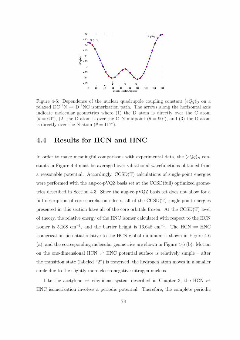
Figure 4-5: Dependence of the nuclear quadrupole coupling constant (eQq)D on arelaxed DC15N D15NC isomerization path. The arrows along the horizontal axisindicate molecular geometries where (1) the D atom is directly over the C atom(θ = 60), (2) the D atom is over the C–N midpoint (θ = 90), and (3) the D atomis directly over the N atom (θ = 117).
4.4 Results for HCN and HNC
In order to make meaningful comparisons with experimental data, the (eQq)N con-
stants in Figure 4-4 must be averaged over vibrational wavefunctions obtained from
a reasonable potential. Accordingly, CCSD(T) calculations of single-point energies
were performed with the aug-cc-pVQZ basis set at the CCSD(full) optimized geome-
tries described in Section 4.3. Since the aug-cc-pVQZ basis set does not allow for a
full description of core correlation effects, all of the CCSD(T) single-point energies
presented in this section have all of the core orbitals frozen. At the CCSD(T) level
of theory, the relative energy of the HNC isomer calculated with respect to the HCN
isomer is 5,168 cm−1, and the barrier height is 16,648 cm−1. The HCN HNC
isomerization potential relative to the HCN global minimum is shown in Figure 4-6
(a), and the corresponding molecular geometries are shown in Figure 4-6 (b). Motion
on the one-dimensional HCN HNC potential surface is relatively simple – after
the transition state (labeled “2”) is traversed, the hydrogen atom moves in a smaller
circle due to the slightly more electronegative nitrogen nucleus.
Like the acetylene vinylidene system described in Chapter 3, the HCN HNC isomerization involves a periodic potential. Therefore, the complete periodic
78
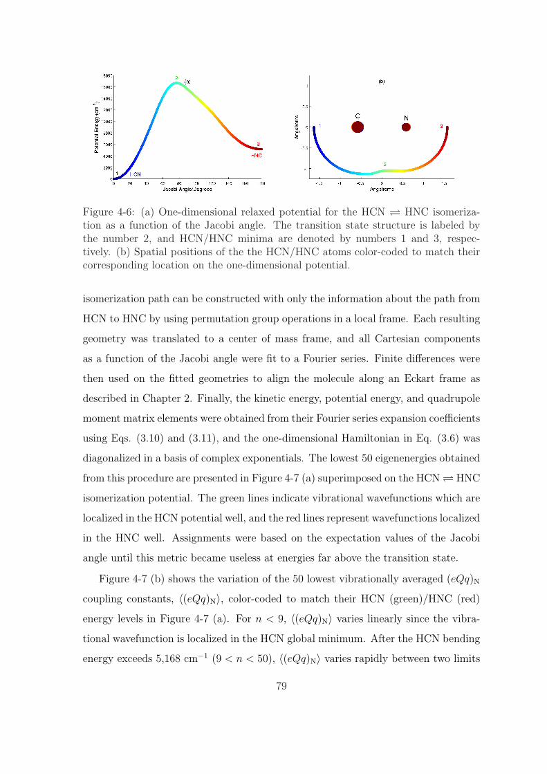
Figure 4-6: (a) One-dimensional relaxed potential for the HCN HNC isomeriza-tion as a function of the Jacobi angle. The transition state structure is labeled bythe number 2, and HCN/HNC minima are denoted by numbers 1 and 3, respec-tively. (b) Spatial positions of the the HCN/HNC atoms color-coded to match theircorresponding location on the one-dimensional potential.
isomerization path can be constructed with only the information about the path from
HCN to HNC by using permutation group operations in a local frame. Each resulting
geometry was translated to a center of mass frame, and all Cartesian components
as a function of the Jacobi angle were fit to a Fourier series. Finite differences were
then used on the fitted geometries to align the molecule along an Eckart frame as
described in Chapter 2. Finally, the kinetic energy, potential energy, and quadrupole
moment matrix elements were obtained from their Fourier series expansion coefficients
using Eqs. (3.10) and (3.11), and the one-dimensional Hamiltonian in Eq. (3.6) was
diagonalized in a basis of complex exponentials. The lowest 50 eigenenergies obtained
from this procedure are presented in Figure 4-7 (a) superimposed on the HCN HNC
isomerization potential. The green lines indicate vibrational wavefunctions which are
localized in the HCN potential well, and the red lines represent wavefunctions localized
in the HNC well. Assignments were based on the expectation values of the Jacobi
angle until this metric became useless at energies far above the transition state.
Figure 4-7 (b) shows the variation of the 50 lowest vibrationally averaged (eQq)N
coupling constants, 〈(eQq)N〉, color-coded to match their HCN (green)/HNC (red)
energy levels in Figure 4-7 (a). For n < 9, 〈(eQq)N〉 varies linearly since the vibra-
tional wavefunction is localized in the HCN global minimum. After the HCN bending
energy exceeds 5,168 cm−1 (9 < n < 50), 〈(eQq)N〉 varies rapidly between two limits
79

Figure 4-7: (a) The 50 lowest vibrational eigenvalues for the HCN HNC potentialobtained at the CCSD(T)/aug-cc-pVQZ level of theory. Each of the eigenvalues isassociated with either HCN (green-colored) or HNC (red-colored) localization. (b)Vibrationally averaged nuclear quadrupole coupling constants for the lowest 50 vi-brational states of HCN (green)/HNC (red) energy.
since the vibrational wavefunction alternates its localization between the local HNC
minimum and the global HCN minimum. Once the bending energy surpasses 16,648
cm−1 (n > 50), the hydrogen migration becomes nearly a free rotation and 〈(eQq)N〉is approximately constant with a limiting value of approximately -4.5 MHz. Figure
4-8 and Table 4.1 compare bending frequencies between the one-dimensional ab initio
model and the experimentally determined (l = 0) frequencies for both HCN and HNC
[84, 85]. Only the experimental frequencies for even quanta in the bend are presented
since vibrations with odd quanta are currently not available. The agreement between
the frequencies is good, and both the HCN and HNC data obey a linear trend with
710.8 cm−1/(HCN bend quantum) and 492.1 cm−1/(HNC bend quantum) respectively
(the experimental data gives smaller slopes of 685.6 cm−1/(HCN bend quantum) and
468.4 cm−1/(HNC bend quantum)). Similarly, Figure 4-9 and Table 4.2 present the
dependence of the vibrationally averaged (eQq)N values as a function of vibrational
excitation for both HCN and HNC. Experimental quadrupole coupling constants were
taken from both Bechtel et al. [86] and experiments currently in progress. The vibra-
tionally averaged quadrupole coupling constants also obey a nearly linear trend with
-0.062 MHz/(HCN bend quantum) and -0.157 MHz/(HNC bend quantum). These
values are in fair agreement with the experimental findings of Bechtel and coworkers
who measure coupling constants of -0.075 MHz/(HCN bend quantum) and -0.118
80
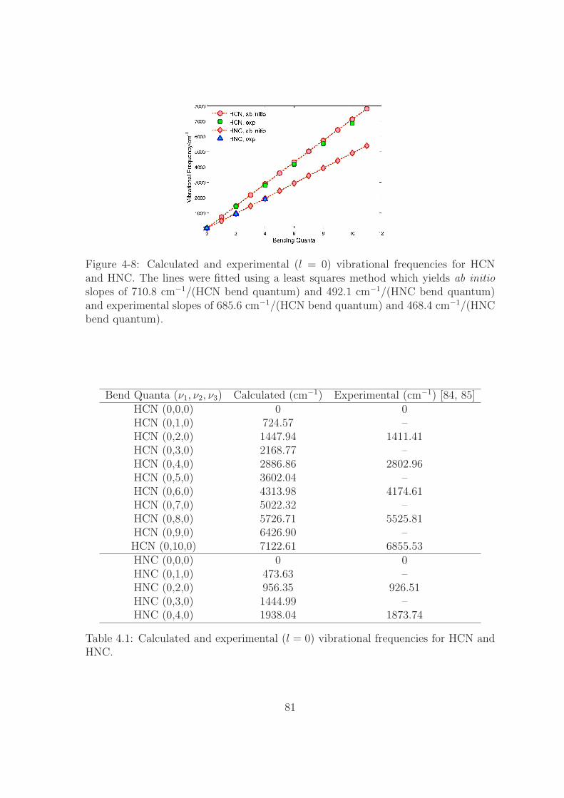
Figure 4-8: Calculated and experimental (l = 0) vibrational frequencies for HCNand HNC. The lines were fitted using a least squares method which yields ab initioslopes of 710.8 cm−1/(HCN bend quantum) and 492.1 cm−1/(HNC bend quantum)and experimental slopes of 685.6 cm−1/(HCN bend quantum) and 468.4 cm−1/(HNCbend quantum).
Bend Quanta (ν1, ν2, ν3) Calculated (cm−1) Experimental (cm−1) [84, 85]HCN (0,0,0) 0 0HCN (0,1,0) 724.57 –HCN (0,2,0) 1447.94 1411.41HCN (0,3,0) 2168.77 –HCN (0,4,0) 2886.86 2802.96HCN (0,5,0) 3602.04 –HCN (0,6,0) 4313.98 4174.61HCN (0,7,0) 5022.32 –HCN (0,8,0) 5726.71 5525.81HCN (0,9,0) 6426.90 –HCN (0,10,0) 7122.61 6855.53HNC (0,0,0) 0 0HNC (0,1,0) 473.63 –HNC (0,2,0) 956.35 926.51HNC (0,3,0) 1444.99 –HNC (0,4,0) 1938.04 1873.74
Table 4.1: Calculated and experimental (l = 0) vibrational frequencies for HCN andHNC.
81

Figure 4-9: Calculated and experimental (l = 0) nuclear quadrupole coupling con-stants for HCN and HNC. The lines were fitted using a least squares method whichyields ab initio slopes of -0.062 MHz/(HCN bend quantum) and -0.157 MHz/(HNCbend quantum) and experimental slopes of -0.075 MHz/(HCN bend quantum) and-0.118 MHz/(HNC bend quantum). Dr. Hans A. Bechtel is acknowledged for provid-ing the experimental quadrupole coupling constants.
Bend Quanta (ν1, ν2, ν3) Calculated (MHz) Experimental (MHz) [86]HCN (0,0,0) -4.7545 -4.7084HCN (0,1,0) -4.8223 –HCN (0,2,0) -4.8887 -4.8966HCN (0,3,0) -4.9543 –HCN (0,4,0) -5.0189 -5.0699HCN (0,5,0) -5.0822 –HCN (0,6,0) -5.1444 -5.2175HCN (0,7,0) -5.2054 –HCN (0,8,0) -5.2654 -5.3485HCN (0,9,0) -5.3242 –HCN (0,10,0) -5.3818 -5.4579HNC (0,0,0) 0.2607 0.2641HNC (0,1,0) 0.1094 –HNC (0,2,0) -0.0418 0.0000HNC (0,3,0) -0.1933 –HNC (0,4,0) -0.3459 -0.2066
Table 4.2: Calculated and experimental (l = 0) nuclear quadrupole coupling con-stants for HCN and HNC. Dr. Hans A. Bechtel is acknowledged for providing theexperimental quadrupole coupling constants.
82

MHz/(HNC bend quantum). Further studies on higher vibrational states and hyper-
fine measurements on other isotopomers are currently in progress.
4.5 Conclusion
This chapter has demonstrated that the hyperfine structures of HCN and HNC are
considerably different and can be used as a sensitive probe for the onset of isomer-
ization. In particular, it was shown that the calculated nuclear quadrupole coupling
constants at the CCSD(full) level change significantly, even with minor changes in
the geometry. Consequently, comparisons with the available experimental data indi-
cate that it is not sufficient to study only the HCN/HNC minima, and vibrational
averaging of the entire isomerization path is necessary.
In addition, to obtain quantitative agreement with experiment, it appears that
large core valence basis sets are necessary to describe the electric field gradients at the
nuclei of interest. Using these basis sets for the DC15N and C15NC isotopomers, small
coupling constants were calculated, which arise from the nearly symmetrical chemical
environment experienced by the deuteron nucleus during the isomerization process.
On the other hand, the large 14N quadrupole coupling constant, in the vicinity of
the HCN potential well, makes it an ideal system for millimeter wave spectroscopic
studies. Furthermore, the direct comparison between vibrationally averaged (eQq)N
values with available experimental data demonstrates that the nuclear quadrupole
couplings can be adequately predicted by ab initio quantum chemical methods. It is
clear, however, that it may be necessary to consider the anharmonic couplings to the
other modes in order to obtain better estimates of vibrationally averaged quantities.
83

84
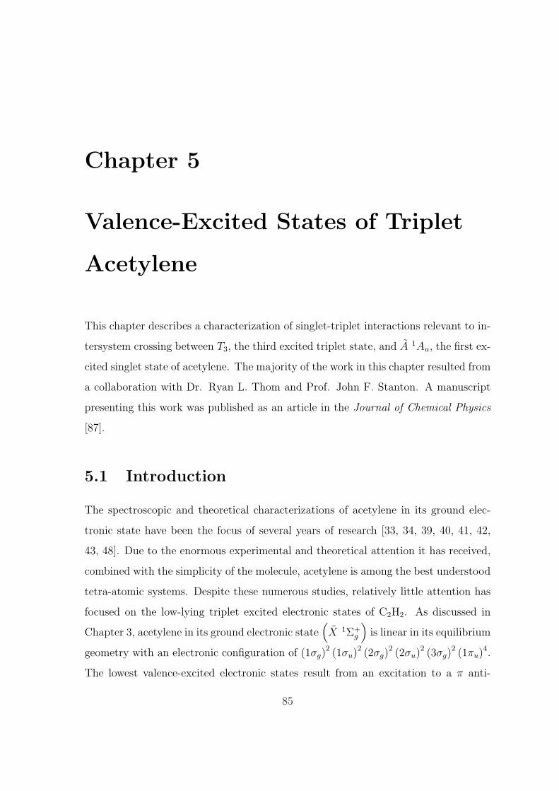
Chapter 5
Valence-Excited States of Triplet
Acetylene
This chapter describes a characterization of singlet-triplet interactions relevant to in-
tersystem crossing between T3, the third excited triplet state, and A 1Au, the first ex-
cited singlet state of acetylene. The majority of the work in this chapter resulted from
a collaboration with Dr. Ryan L. Thom and Prof. John F. Stanton. A manuscript
presenting this work was published as an article in the Journal of Chemical Physics
[87].
5.1 Introduction
The spectroscopic and theoretical characterizations of acetylene in its ground elec-
tronic state have been the focus of several years of research [33, 34, 39, 40, 41, 42,
43, 48]. Due to the enormous experimental and theoretical attention it has received,
combined with the simplicity of the molecule, acetylene is among the best understood
tetra-atomic systems. Despite these numerous studies, relatively little attention has
focused on the low-lying triplet excited electronic states of C2H2. As discussed in
Chapter 3, acetylene in its ground electronic state(X 1Σ+
g
)is linear in its equilibrium
geometry with an electronic configuration of (1σg)2 (1σu)
2 (2σg)2 (2σu)
2 (3σg)2 (1πu)
4.
The lowest valence-excited electronic states result from an excitation to a π anti-
85

Figure 5-1: Highest occupied molecular orbital for the S11Au trans state of acetylene.
bonding orbital within the π4 → π3π∗ manifold. As a result, these orbital excitations
in acetylene are stabilized by having both CCH bond angles bend out of linearity. For
example, the first excited singlet state of acetylene(A 1Au
)is trans bent, and Figure
5-1 depicts the highest occupied molecular orbital for this optimized geometry. Fig-
ure 5-2 shows the potential energy surfaces for several low-lying acetylene electronic
states, all constrained to planar geometry and plotted as a function of the CCH bend
coordinate. From Figure 5-2, the first triplet potential surface (T1) possesses stable
minima in both trans- and cis-bent geometries, denoted by 3Bu and 3B2 respectively.
The second triplet state (T2) also supports both trans- and cis- minima (3Bu and
3B2 respectively) with the cis stationary point being more stable. The stationary
points on the T3 surface are not well characterized but play an important role for
interpreting the Zeeman anticrossing (ZAC) measurements by Dupre and coworkers
[1, 88, 89, 90], described further in Section 5.2.
In this chapter, a new ab initio study of the acetylene T3 potential surface is
reported, which clarifies the nature of its energy minimum. The resulting equilibrium
geometries and diabatic force constants enable an analysis of interactions between
T3 vibrational levels which are energetically near the 3ν3 vibrational level on the S1
excited singlet state. The following sections describe theoretical assignments and
comparisons with experimental data to resolve some of the existing controversies
concerning the photophysics of this T3 state.
86
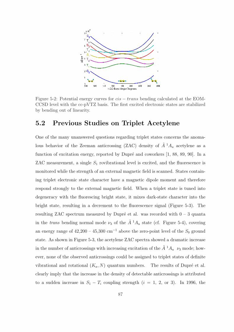
Figure 5-2: Potential energy curves for cis− trans bending calculated at the EOM-CCSD level with the cc-pVTZ basis. The first excited electronic states are stabilizedby bending out of linearity.
5.2 Previous Studies on Triplet Acetylene
One of the many unanswered questions regarding triplet states concerns the anoma-
lous behavior of the Zeeman anticrossing (ZAC) density of A 1Au acetylene as a
function of excitation energy, reported by Dupre and coworkers [1, 88, 89, 90]. In a
ZAC measurement, a single S1 rovibrational level is excited, and the fluorescence is
monitored while the strength of an external magnetic field is scanned. States contain-
ing triplet electronic state character have a magnetic dipole moment and therefore
respond strongly to the external magnetic field. When a triplet state is tuned into
degeneracy with the fluorescing bright state, it mixes dark-state character into the
bright state, resulting in a decrement to the fluorescence signal (Figure 5-3). The
resulting ZAC spectrum measured by Dupre et al. was recorded with 0 – 3 quanta
in the trans bending normal mode ν3 of the A 1Au state (cf. Figure 5-4), covering
an energy range of 42,200 – 45,300 cm−1 above the zero-point level of the S0 ground
state. As shown in Figure 5-3, the acetylene ZAC spectra showed a dramatic increase
in the number of anticrossings with increasing excitation of the A 1Au ν3 mode; how-
ever, none of the observed anticrossings could be assigned to triplet states of definite
vibrational and rotational (Ka, N) quantum numbers. The results of Dupre et al.
clearly imply that the increase in the density of detectable anticrossings is attributed
to a sudden increase in S1 − Ti coupling strength (i = 1, 2, or 3). In 1996, the
87
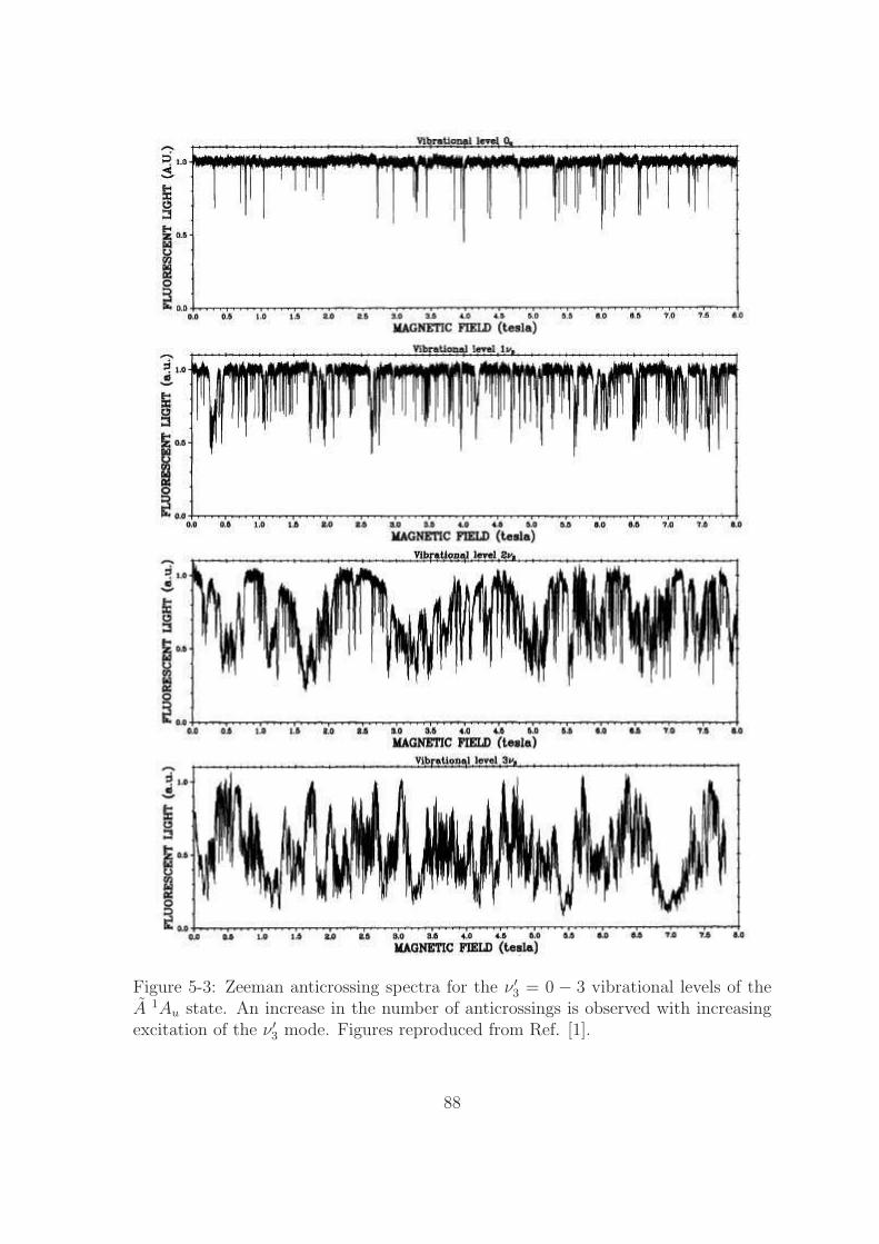
Figure 5-3: Zeeman anticrossing spectra for the ν ′3 = 0 − 3 vibrational levels of theA 1Au state. An increase in the number of anticrossings is observed with increasingexcitation of the ν ′3 mode. Figures reproduced from Ref. [1].
88

Figure 5-4: The ν3 (ag) trans-bending normal mode for the A 1Au state of acetylene.The harmonic vibrational frequency was calculated at the EOM-CCSD level with thecc-pVQZ basis.
anomalous ZAC density was partially addressed in the work by Vacek et al. [91] and
Sherrill et al. [92] who concluded that the T1 and T2 states are not candidates for
the triplet coupling state since they are energetically too low and outside the experi-
mental ZAC window. Consequently, several studies [93, 94, 95] have focused on the
third triplet electronic state (T3) as the most likely candidate for providing the special
“doorway” to coupling with the 3ν3 vibrational level of S1. One of the most extensive
analyses attempting to assign the triplet perturbers of S1 3ν3 is the work by Mishra
and coworkers [96] who simultaneously recorded ultraviolet laser-induced fluorescence
(UV-LIF) and surface electron ejection by laser excited metastables (SEELEM) spec-
tra in the 45,300 cm−1 region. One of the key results of that work is the identification
of a rotational series of triplet levels which were fitted using a deperturbation model.
In contrast to the several experimental studies in the literature, ab initio electronic
structure calculations have been slow in characterizing the location and nature of the
minimum of the T3 potential energy surface. Cui et al. [97, 98] were only able to
locate a transition state (saddle point), with one imaginary normal-mode frequency
along an antisymmetric CCH bending coordinate (see Figures 5-7 (a)–(b)). More
recently, Ventura et al. [99] performed extended multireference electron correlation
calculations on all four of the lowest-lying acetylene triplet potential energy surfaces.
These authors were the first researchers to report a genuine minimum (no imaginary
frequencies) belonging to the T3 surface. Although Ventura et al. give an optimized
geometry for this equilibrium structure (which has a similar geometry to the saddle
89
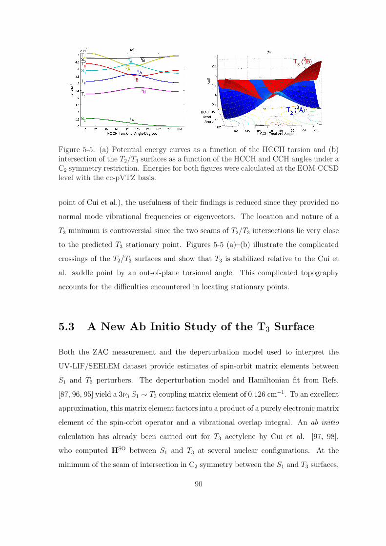
Figure 5-5: (a) Potential energy curves as a function of the HCCH torsion and (b)intersection of the T2/T3 surfaces as a function of the HCCH and CCH angles under aC2 symmetry restriction. Energies for both figures were calculated at the EOM-CCSDlevel with the cc-pVTZ basis.
point of Cui et al.), the usefulness of their findings is reduced since they provided no
normal mode vibrational frequencies or eigenvectors. The location and nature of a
T3 minimum is controversial since the two seams of T2/T3 intersections lie very close
to the predicted T3 stationary point. Figures 5-5 (a)–(b) illustrate the complicated
crossings of the T2/T3 surfaces and show that T3 is stabilized relative to the Cui et
al. saddle point by an out-of-plane torsional angle. This complicated topography
accounts for the difficulties encountered in locating stationary points.
5.3 A New Ab Initio Study of the T3 Surface
Both the ZAC measurement and the deperturbation model used to interpret the
UV-LIF/SEELEM dataset provide estimates of spin-orbit matrix elements between
S1 and T3 perturbers. The deperturbation model and Hamiltonian fit from Refs.
[87, 96, 95] yield a 3ν3 S1 ∼ T3 coupling matrix element of 0.126 cm−1. To an excellent
approximation, this matrix element factors into a product of a purely electronic matrix
element of the spin-orbit operator and a vibrational overlap integral. An ab initio
calculation has already been carried out for T3 acetylene by Cui et al. [97, 98],
who computed HSO between S1 and T3 at several nuclear configurations. At the
minimum of the seam of intersection in C2 symmetry between the S1 and T3 surfaces,
90
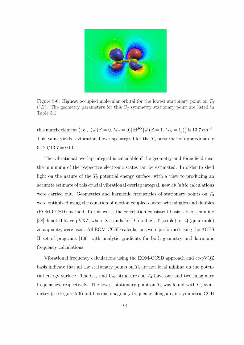
Figure 5-6: Highest occupied molecular orbital for the lowest stationary point on T3
(3B). The geometry parameters for this C2 symmetry stationary point are listed inTable 5.1.
this matrix element(i.e., 〈Ψ (S = 0,MS = 0)|HSO |Ψ (S = 1, MS = 1)〉) is 13.7 cm−1.
This value yields a vibrational overlap integral for the T3 perturber of approximately
0.126/13.7 = 0.01.
The vibrational overlap integral is calculable if the geometry and force field near
the minimum of the respective electronic states can be estimated. In order to shed
light on the nature of the T3 potential energy surface, with a view to producing an
accurate estimate of this crucial vibrational overlap integral, new ab initio calculations
were carried out. Geometries and harmonic frequencies of stationary points on T3
were optimized using the equation of motion coupled cluster with singles and doubles
(EOM-CCSD) method. In this work, the correlation-consistent basis sets of Dunning
[38] denoted by cc-pVXZ, where X stands for D (double), T (triple), or Q (quadruple)
zeta quality, were used. All EOM-CCSD calculations were performed using the ACES
II set of programs [100] with analytic gradients for both geometry and harmonic
frequency calculations.
Vibrational frequency calculations using the EOM-CCSD approach and cc-pVQZ
basis indicate that all the stationary points on T3 are not local minima on the poten-
tial energy surface. The C2h and C2v structures on T3 have one and two imaginary
frequencies, respectively. The lowest stationary point on T3 was found with C2 sym-
metry (see Figure 5-6) but has one imaginary frequency along an antisymmetric CCH
91

Figure 5-7: (a) The ν6 antisymmetric CCH bending normal mode for T3 acetylene(∠H1C1C2 = θeq −∆θ, ∠H2C2C1 = θeq + ∆θ) and (b) adiabatic T2/T3 surfaces as afunction of the HCCH torsional angle and CCH asymmetric bend angle. The T2/T3
energies were obtained at the EOM-CCSD level with the cc-pVTZ basis. The sta-tionary point on T3 is unstable against increasing ∆θ.
bending coordinate. In addition, it was found that both T2 and T3 cross at a geom-
etry which is very close to this T3 C2 point. In Figures 5-7 (a)–(b), the effect of
antisymmetric bending on T2 and T3 is shown. Near the T3 C2 stationary point, the
energy decreases on antisymmetric bending for the lower state (T3) and increases for
the upper one (T2). The small energy difference between T2 and T3 in Figure 5-7
(b) clearly shows that these two states are better described as coupled surfaces in a
diabatic representation.
5.4 A Brief Digression on Adiabatic and Diabatic
Representations
Before proceeding with a detailed analysis of the T2/T3 diabatization, it is helpful to
first consider a simple example of a model Hamiltonian which contains vibrational-
electronic (vibronic) couplings between electronic states with the vibrational normal
modes. One way to visualize the adiabatic and diabatic states is to look at a one-
dimensional slice of Figure 5-7 (b) along the asymmetric bending coordinate. In
Figure 5-8, the solid lines represent two typical potential energy curves for different
adiabatic electronic states that one would obtain from a quantum chemistry ap-
92
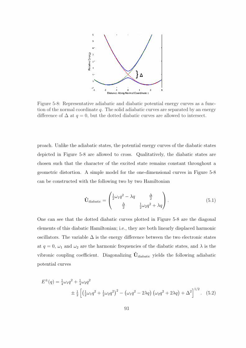
Figure 5-8: Representative adiabatic and diabatic potential energy curves as a func-tion of the normal coordinate q. The solid adiabatic curves are separated by an energydifference of ∆ at q = 0, but the dotted diabatic curves are allowed to intersect.
proach. Unlike the adiabatic states, the potential energy curves of the diabatic states
depicted in Figure 5-8 are allowed to cross. Qualitatively, the diabatic states are
chosen such that the character of the excited state remains constant throughout a
geometric distortion. A simple model for the one-dimensional curves in Figure 5-8
can be constructed with the following two by two Hamiltonian
Udiabatic =
12ω1q
2 − λq ∆2
∆2
12ω2q
2 + λq
. (5.1)
One can see that the dotted diabatic curves plotted in Figure 5-8 are the diagonal
elements of this diabatic Hamiltonian; i.e., they are both linearly displaced harmonic
oscillators. The variable ∆ is the energy difference between the two electronic states
at q = 0, ω1 and ω2 are the harmonic frequencies of the diabatic states, and λ is the
vibronic coupling coefficient. Diagonalizing Udiabatic yields the following adiabatic
potential curves
E±(q) = 14ω1q
2 + 14ω2q
2
± 12
[(12ω1q
2 + 12ω2q
2)2 − (
ω1q2 − 2λq
) (ω2q
2 + 2λq)
+ ∆2]1/2
. (5.2)
93
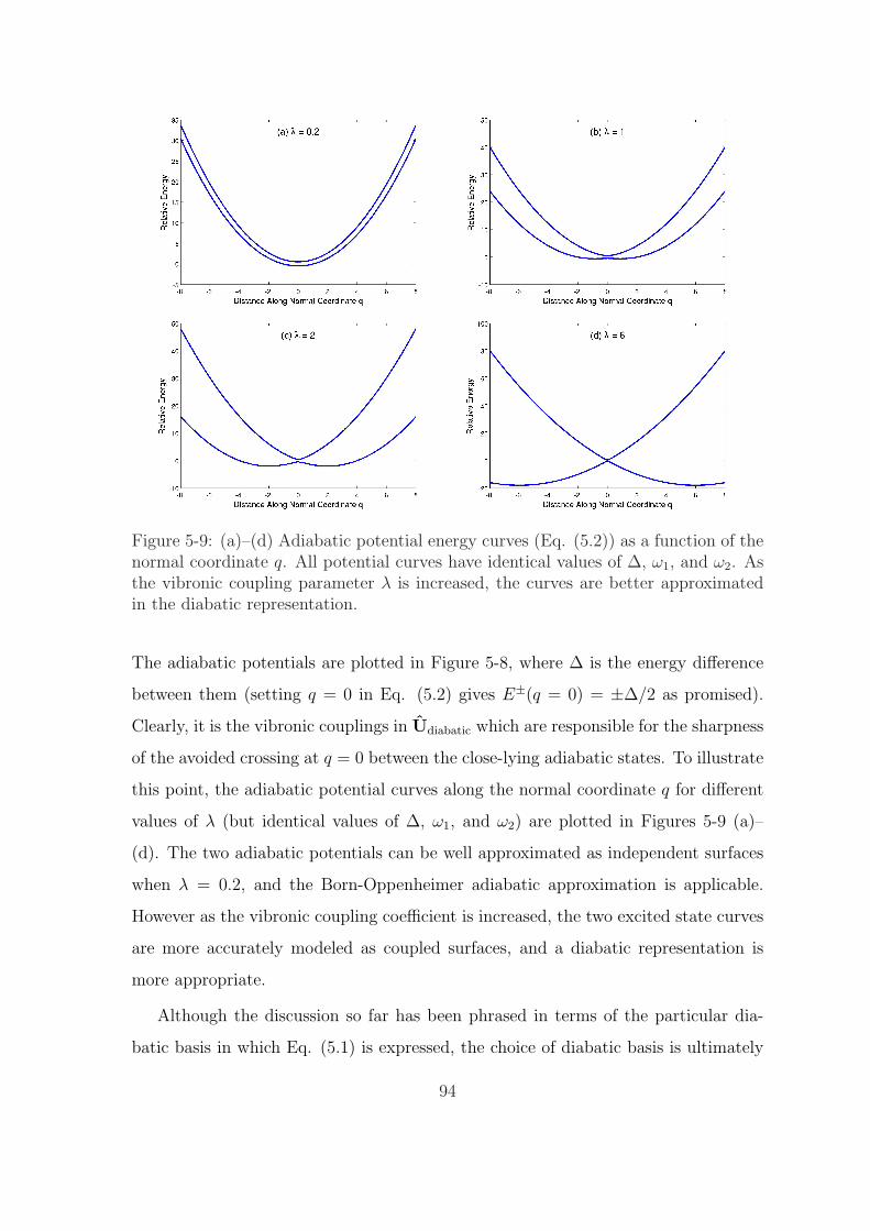
Figure 5-9: (a)–(d) Adiabatic potential energy curves (Eq. (5.2)) as a function of thenormal coordinate q. All potential curves have identical values of ∆, ω1, and ω2. Asthe vibronic coupling parameter λ is increased, the curves are better approximatedin the diabatic representation.
The adiabatic potentials are plotted in Figure 5-8, where ∆ is the energy difference
between them (setting q = 0 in Eq. (5.2) gives E±(q = 0) = ±∆/2 as promised).
Clearly, it is the vibronic couplings in Udiabatic which are responsible for the sharpness
of the avoided crossing at q = 0 between the close-lying adiabatic states. To illustrate
this point, the adiabatic potential curves along the normal coordinate q for different
values of λ (but identical values of ∆, ω1, and ω2) are plotted in Figures 5-9 (a)–
(d). The two adiabatic potentials can be well approximated as independent surfaces
when λ = 0.2, and the Born-Oppenheimer adiabatic approximation is applicable.
However as the vibronic coupling coefficient is increased, the two excited state curves
are more accurately modeled as coupled surfaces, and a diabatic representation is
more appropriate.
Although the discussion so far has been phrased in terms of the particular dia-
batic basis in which Eq. (5.1) is expressed, the choice of diabatic basis is ultimately
94

Figure 5-10: Diabatic potential energy curves represented in the new basis of Eq.(5.4).
immaterial. For example, consider another diabatic basis that is obtained from the
previous basis by the unitary matrix
S =1√2
1 1
1 −1
. (5.3)
The Hamiltonian in this new diabatic basis is obtained by performing the same unitary
transformation on the old Hamiltonian
Unewdiabatic = S−1UdiabaticS
=
ω1+ω2
4q2 + ∆
2ω1−ω2
4q2 − λq
ω1−ω2
4q2 − λq ω1+ω2
4q2 − ∆
2
.
(5.4)
Once again, the new diabatic states are the diagonal elements of Unewdiabatic which are
plotted in Figure 5-10. Although the new diabatic states look considerably different
than the curves plotted in Figure 5-8, diagonalization of Unewdiabatic still yields the same
adiabatic potential curves depicted in Figure 5-8 and also mathematically expressed
in Eq. (5.2) (the adiabatic potentials must be the same since the eigenvalues are
invariant under a unitary transformation). Evidently, the old diabatic basis states
shown in Figure 5-8 are equally as valid as the new diabatic basis states in Figure
5-10 since they both preserve the same adiabatic eigenvalues. The only criterion for
the diabatic states is that they preserve their character upon geometric distortion, a
95

behavior which is still clearly demonstrated in Figure 5-10. Consequently, the choice
of a diabatic basis is completely arbitrary and not unique; in practice, the basis which
is chosen is usually the one in which the electronic states can be computed with the
least amount of effort. In the next section,the diabatic basis in which Eq. (5.4) is
expressed will be utilized to obtain the (non-imaginary) diabatic frequencies of T2/T3
acetylene.
5.5 The T2/T3 Vibronic Model
To treat the interactions between T2 and T3, a two-dimensional diabatic model was
used in which the T3 and T2 electronic states are coupled by the two nontotally
symmetric modes, ν5 (antisymmetric CC stretch) and ν6 (antisymmetric CCH bend)
(see Figures 5-11 (e)–(f)). To estimate the adiabatic couplings, the diabatic electronic
Hamiltonian matrix U is written in the basis spanned by φ1 and φ2, which are the
diabatic wavefunctions associated with T3 and T2, respectively. Within the harmonic
approximation, the diabatic potential energy curves U11 and U22 expressed in the
dimensionless normal coordinates q = (ω/~)1/2Q are given by
U11 = 〈φ1|U |φ1〉 =1
2ω5q
25 +
1
2ω6q
26, (5.5)
U22 = 〈φ2|U |φ2〉 =1
2ω5q
25 +
1
2ω6q
26 + ∆, (5.6)
where ∆ is the vertical excitation energy between the T3 and T2 states at the reference
C2 saddle point on the T3 surface. In Eq. (5.5), mode ν5 is assumed to have the
same diabatic frequency (ω5) on the T3 and T2 diabatic surfaces [101, 102]. This
assumption is quite reasonable given that the potential energy surfaces for T2 and T3
are symmetrical about the plane ∠HCC = θeq = 137 in Figure 5-7 (b) (i.e., the local
minima on the lower surface have the same curvature). Similarly, mode ν6 is assumed
to have the same diabatic frequency (ω6) on the T3 and T2 diabatic surfaces. By
choosing ω5 (or ω6) to have the same frequency on the T3 and T2 diabatic surfaces,
the diabatic frequencies obtained from the basis in which Eq. (5.4) is expressed
96
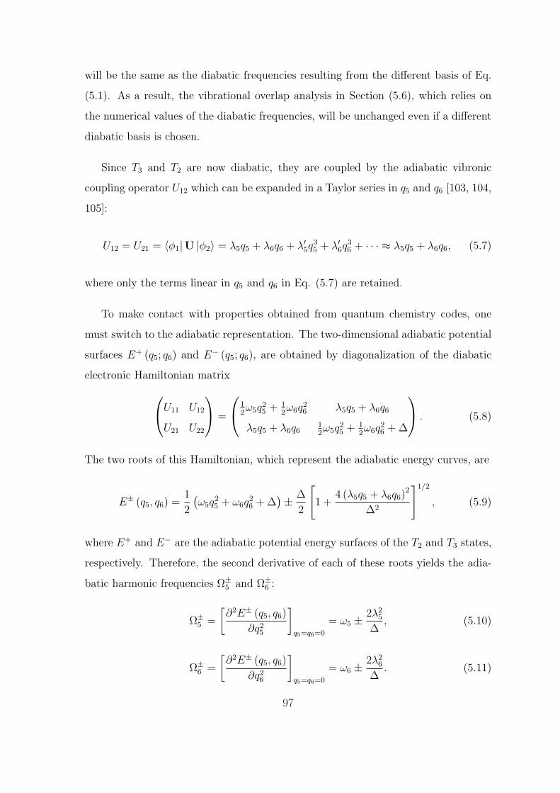
will be the same as the diabatic frequencies resulting from the different basis of Eq.
(5.1). As a result, the vibrational overlap analysis in Section (5.6), which relies on
the numerical values of the diabatic frequencies, will be unchanged even if a different
diabatic basis is chosen.
Since T3 and T2 are now diabatic, they are coupled by the adiabatic vibronic
coupling operator U12 which can be expanded in a Taylor series in q5 and q6 [103, 104,
105]:
U12 = U21 = 〈φ1|U |φ2〉 = λ5q5 + λ6q6 + λ′5q35 + λ′6q
36 + · · · ≈ λ5q5 + λ6q6, (5.7)
where only the terms linear in q5 and q6 in Eq. (5.7) are retained.
To make contact with properties obtained from quantum chemistry codes, one
must switch to the adiabatic representation. The two-dimensional adiabatic potential
surfaces E+ (q5; q6) and E− (q5; q6), are obtained by diagonalization of the diabatic
electronic Hamiltonian matrix
U11 U12
U21 U22
=
12ω5q
25 + 1
2ω6q
26 λ5q5 + λ6q6
λ5q5 + λ6q612ω5q
25 + 1
2ω6q
26 + ∆
. (5.8)
The two roots of this Hamiltonian, which represent the adiabatic energy curves, are
E± (q5, q6) =1
2
(ω5q
25 + ω6q
26 + ∆
)± ∆
2
[1 +
4 (λ5q5 + λ6q6)2
∆2
]1/2
, (5.9)
where E+ and E− are the adiabatic potential energy surfaces of the T2 and T3 states,
respectively. Therefore, the second derivative of each of these roots yields the adia-
batic harmonic frequencies Ω±5 and Ω±
6 :
Ω±5 =
[∂2E± (q5, q6)
∂q25
]
q5=q6=0
= ω5 ± 2λ25
∆, (5.10)
Ω±6 =
[∂2E± (q5, q6)
∂q26
]
q5=q6=0
= ω6 ± 2λ26
∆. (5.11)
97
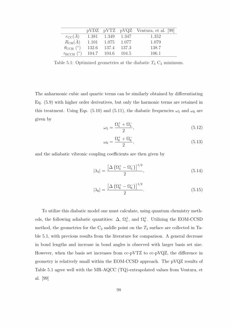
pVDZ pVTZ pVQZ Ventura, et al. [99]
rCC(A) 1.381 1.349 1.347 1.352RCH(A) 1.101 1.075 1.077 1.079θCCH () 132.6 137.4 137.3 138.7τHCCH () 104.7 104.6 104.5 106.1
Table 5.1: Optimized geometries at the diabatic T3 C2 minimum.
The anharmonic cubic and quartic terms can be similarly obtained by differentiating
Eq. (5.9) with higher order derivatives, but only the harmonic terms are retained in
this treatment. Using Eqs. (5.10) and (5.11), the diabatic frequencies ω5 and ω6 are
given by
ω5 =Ω+
5 + Ω−5
2, (5.12)
ω6 =Ω+
6 + Ω−6
2, (5.13)
and the adiabatic vibronic coupling coefficients are then given by
|λ5| =[∆
(Ω+
5 − Ω−5
)]1/2
2, (5.14)
|λ6| =[∆
(Ω+
6 − Ω−6
)]1/2
2. (5.15)
To utilize this diabatic model one must calculate, using quantum chemistry meth-
ods, the following adiabatic quantities: ∆, Ω±5 , and Ω±
6 . Utilizing the EOM-CCSD
method, the geometries for the C2 saddle point on the T3 surface are collected in Ta-
ble 5.1, with previous results from the literature for comparison. A general decrease
in bond lengths and increase in bond angles is observed with larger basis set size.
However, when the basis set increases from cc-pVTZ to cc-pVQZ, the difference in
geometry is relatively small within the EOM-CCSD approach. The pVQZ results of
Table 5.1 agree well with the MR-AQCC (TQ)-extrapolated values from Ventura, et
al. [99]
98

pVDZ pVTZ pVQZ∆ (eV) 0.0461 0.0296 0.0281|λ5| (eV) 0.0308 0.0226 0.0220|λ6| (eV) 1.101 1.075 1.024ω5 (cm−1) 2965.0 3041.7 3036.5ω6 (cm−1) 474.6 370.4 397.6
Table 5.2: Ab initio adiabatic coupling parameters between T3 and T2 with diabaticfrequencies of T3.
5.6 S1/T3 Vibrational Overlap Integrals
The computed parameters for the adiabatic vibronic couplings between T3 and T2
were obtained using Eqs. (5.14) and (5.15), and are listed in Table 5.2. The diabatic
frequencies of T3, ω5 and ω6, (rescaled to conventional mass-weighted normal coordi-
nates) are also listed. Within all basis sets, the ν6 mode, which corresponds to the
antisymmetric CCH bend, provides the stronger coupling between T3 and T2.
Now the non-imaginary harmonic frequencies and force constants about the di-
abatized T3 minimum can be used to compute vibrational overlap integrals with S1
3ν3. In order to minimize errors and maintain consistency within the calculation, the
harmonic frequencies and force constants for S1 were recomputed within the EOM-
CCSD approach. Table 5.3 lists the normal modes and calculated frequencies for S1
(It is worth mentioning that the EOM-CCSD approach is not strictly appropriate
for calculating S1 properties because of the multireference character of the reference
ground state wavefunction. This is reflected in the calculated ν4 frequency of 641.5
cm−1 which is noticeably smaller than 765 cm−1 obtained from experiment. The S1
vibrational frequencies obtained using other approaches are currently being investi-
gated by Prof. John F. Stanton and Bryan M. Wong.) The calculation also establishes
an electronic energy separation (S1 − T3) of 0.0012211 Hartree = 270 cm−1 using the
cc-pVQZ basis.
The vibrational overlap integrals between T3 and S1 3ν3 can be calculated within
the harmonic oscillator approximation using the multidimensional generating function
formalism developed by Sharp and Rosenstock [108] and extended by several other
authors [109, 110]. The original manuscript by Sharp and Rosenstock, it should
99
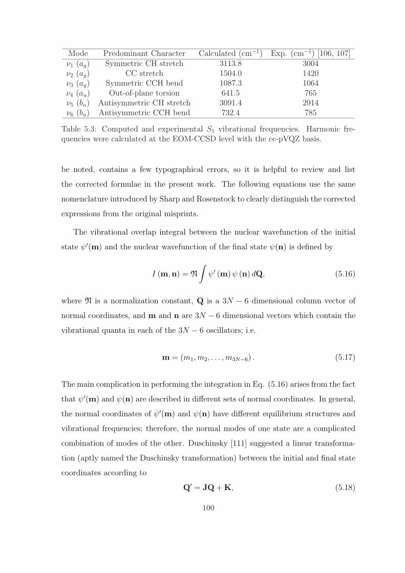
Mode Predominant Character Calculated (cm−1) Exp. (cm−1) [106, 107]ν1 (ag) Symmetric CH stretch 3113.8 3004ν2 (ag) CC stretch 1504.0 1420ν3 (ag) Symmetric CCH bend 1087.3 1064ν4 (au) Out-of-plane torsion 641.5 765ν5 (bu) Antisymmetric CH stretch 3091.4 2914ν6 (bu) Antisymmetric CCH bend 732.4 785
Table 5.3: Computed and experimental S1 vibrational frequencies. Harmonic fre-quencies were calculated at the EOM-CCSD level with the cc-pVQZ basis.
be noted, contains a few typographical errors, so it is helpful to review and list
the corrected formulae in the present work. The following equations use the same
nomenclature introduced by Sharp and Rosenstock to clearly distinguish the corrected
expressions from the original misprints.
The vibrational overlap integral between the nuclear wavefunction of the initial
state ψ′(m) and the nuclear wavefunction of the final state ψ(n) is defined by
I (m,n) = N
∫ψ′ (m) ψ (n) dQ, (5.16)
where N is a normalization constant, Q is a 3N − 6 dimensional column vector of
normal coordinates, and m and n are 3N − 6 dimensional vectors which contain the
vibrational quanta in each of the 3N − 6 oscillators; i.e.
m = (m1,m2, . . . , m3N−6) . (5.17)
The main complication in performing the integration in Eq. (5.16) arises from the fact
that ψ′(m) and ψ(n) are described in different sets of normal coordinates. In general,
the normal coordinates of ψ′(m) and ψ(n) have different equilibrium structures and
vibrational frequencies; therefore, the normal modes of one state are a complicated
combination of modes of the other. Duschinsky [111] suggested a linear transforma-
tion (aptly named the Duschinsky transformation) between the initial and final state
coordinates according to
Q′ = JQ + K, (5.18)
100

where the Duschinsky rotation matrix J describes the projection of the normal coor-
dinate basis vectors of the initial state onto those of the final state, and K relates the
difference in molecular geometry between initial and final states
J = (L′)−1L, (5.19)
K = (L′)−1R, (5.20)
In Eqs. (5.19)–(5.20) L is the matrix which relates the normal mode coordinates
Q to the 3N − 6 dimensional column vector of internal displacement coordinates S;
i.e. bond lengths, bond angles, and torsional angles measured with respect to the
equilibrium reference configuration:
S = LQ. (5.21)
In Eq. (5.20), R is the 3N − 6 dimensional vector whose components are the changes
in equilibrium position from the initial to the final states R = Req −R′eq. A lengthy
derivation by Sharp and Rosenstock yields the desired vibrational overlap integrals,
I(m,n), as coefficients in the power series
∑m
∑n
TmUn (2m2n/m!n!)1/2 I (m,n) =
I0 exp(T†AT + T†B + U†CU + U†D + U†ET
). (5.22)
A misprint occurs in Eq. (22) of Ref. [108] where the root of the fraction in the
left hand side of the equation is missing. The corrected version is printed above.
Eq. (5.22) is written in the extremely compact notation of Ref. [108] which requires
further explanation. The shorthand notation introduced by Sharp and Rosenstock is
m! =3N−6∏i=1
mi!, (5.23)
101
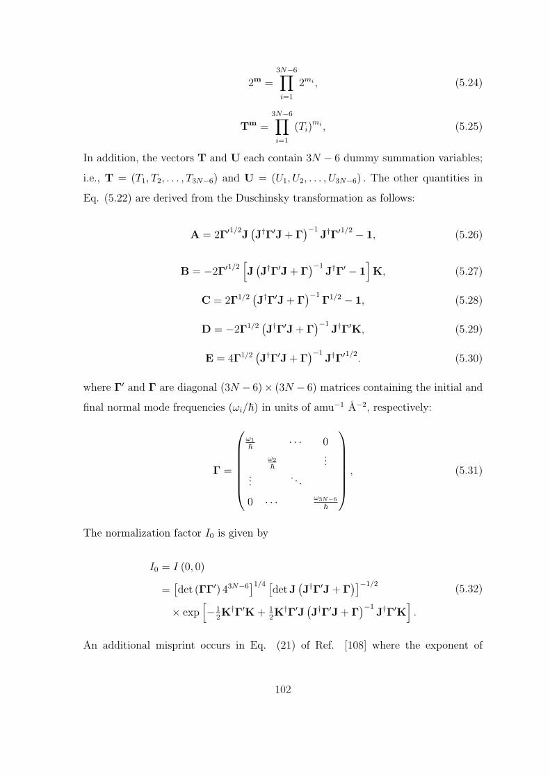
2m =3N−6∏i=1
2mi , (5.24)
Tm =3N−6∏i=1
(Ti)mi , (5.25)
In addition, the vectors T and U each contain 3N − 6 dummy summation variables;
i.e., T = (T1, T2, . . . , T3N−6) and U = (U1, U2, . . . , U3N−6) . The other quantities in
Eq. (5.22) are derived from the Duschinsky transformation as follows:
A = 2Γ′1/2J
(J†Γ′J + Γ
)−1J†Γ′1/2 − 1, (5.26)
B = −2Γ′1/2[J
(J†Γ′J + Γ
)−1J†Γ′ − 1
]K, (5.27)
C = 2Γ1/2(J†Γ′J + Γ
)−1Γ1/2 − 1, (5.28)
D = −2Γ1/2(J†Γ′J + Γ
)−1J†Γ′K, (5.29)
E = 4Γ1/2(J†Γ′J + Γ
)−1J†Γ′1/2
. (5.30)
where Γ′ and Γ are diagonal (3N − 6)× (3N − 6) matrices containing the initial and
final normal mode frequencies (ωi/~) in units of amu−1 A−2, respectively:
Γ =
ω1
~ · · · 0
ω2
~...
.... . .
0 · · · ω3N−6
~
, (5.31)
The normalization factor I0 is given by
I0 = I (0, 0)
=[det (ΓΓ′) 43N−6
]1/4 [detJ
(J†Γ′J + Γ
)]−1/2
× exp[−1
2K†Γ′K + 1
2K†Γ′J
(J†Γ′J + Γ
)−1J†Γ′K
].
(5.32)
An additional misprint occurs in Eq. (21) of Ref. [108] where the exponent of
102

det (ΓΓ′) is incorrect. The corrected version is given by Eq. (5.32) above.
Eq. (5.32) is the main result of Sharp and Rosenstock: to calculate an overlap
integral, I(m,n), the respective sets of quantum numbers m and n are substituted in
Eq. (5.32), and the coefficients of terms at the left and right hand sides with identical
powers of the dummy variables U and T are compared. Unfortunately, the complexity
of the occurring expressions grows rapidly with increasing quantum numbers, and the
procedure of expanding and comparing both sides of Eq. (5.32) becomes extremely
tedious. For the present study of S1/T3 vibrational overlaps, a computer algebra
system was used to obtain the overlap integrals directly by differentiating the Sharp
and Rosenstock generating function with respect to the dummy variables T and U:
I (m,n) = I0 (2m2nm!n!)−1/2
×3N−6∏i=1
∂mi
∂Tmii
∂ni
∂Unii
exp(T†AT + T†B + U†CU + U†D + U†ET
)∣∣∣∣∣T=U=0
. (5.33)
Eq. (5.33) follows directly from the power series definition of I(m,n) expressed
in Eq. (5.32). In a computer program available via the Internet [112], the symbolic
differentiation method has been implemented to calculate vibrational overlap integrals
given L′, L, R′eq, Req, m, and n as inputs for any general molecule. The user-
friendly code and sample inputs for the present S1/T3 study are further documented
in Appendix B.
All that remains is to describe how one may obtain the L matrix found in Eqs.
(5.19)–(5.20). From the FG method of Wilson, Decius, and Cross, [15] the L matrix
is the transformation which simultaneously diagonalizes the G (internal coordinate
momentum coupling) and F (internal coordinate force constant) matrices:
L†G−1L = 1, (5.34)
L†FL = ~2Γ2. (5.35)
The L matrix naturally emerges from a normal mode analysis when the Wilson F
103

matrix is expressed in internal coordinates (i.e. force constants corresponding to
motions directed along valence coordinates). However, the F matrix is not a quantity
which is conventionally computed from ab initio computer codes. Instead, a 3N×3N
Hessian matrix, Fcart, which includes the second partial derivatives of the potential
V with respect to mass-weighted Cartesian displacement of the atoms is produced:
(Fcart)ij =1
(mimj)1/2
∂2V
∂ξi∂ξj
, (5.36)
where ξ1, ξ2, ξ3, . . . , ξ3N are the displacements in Cartesian coordinates ∆x1, ∆y1,
∆z1, . . . , ∆zN , and mi is the mass of the atom to which ξi refers. This 3N × 3N Hes-
sian matrix is usually expressed in a basis where the six zero frequency coordinates
(three translational and three rotational coordinates) have already been projected out.
The diagonalization of the projected Fcart matrix produces 3N − 6, 3N -dimensional
eigenvectors which describe each normal coordinate in terms of mass-weighted Carte-
sian nuclear displacements. These 3N − 6 eigenvectors can be combined to form the
3N × (3N − 6) l matrix:
lik =∂m
1/2i ξi
∂Qk
. (5.37)
Therefore, the L matrix can be obtained from the equation
L = BM−1/2l, (5.38)
where M is a diagonal 3N × 3N matrix of atom masses mi, and B is a (3N −6) × 3N matrix which relates the internal coordinates St to the nuclear Cartesian
displacements:
Btk =∂St
∂ξk
(5.39)
The B matrix is solely dependent on the equilibrium geometry, and its elements
are derived in Eqs. (3), (5)–(7), and (21)–(24) in Section 4-1 of Ref. [15] for bond
stretching, valence angle bending, and torsion respectively (the sets of elements Btk
are denoted by the vector quantities stα in Ref. [15]). The computer source codes,
104

also documented in Appendix B, automatically calculate the B and L matrices in
internal coordinates for acetylene given the equilibrium geometries and l matrices in
Cartesian coordinates.
5.7 Results for T3 Acetylene
The L matrix described in Section 5.6 describes the relative contributions of each
internal coordinate motion to each of the normal mode coordinates. The same in-
formation is expressed more clearly by the orthogonal matrix T (not to be confused
with the vector T in Eqs. (5.22) and (5.25)) defined by
T = G−1/2L (5.40)
where G is the traditional Wilson’s G matrix (effective inverse mass matrix) whose
elements are defined by
Gtt′ =3N∑i=1
1
mi
BtiBt′i (5.41)
The T matrix for the T33B stationary point is presented in Table 5.4, and Table 5.5
lists the symmetries, dominant characters, and frequencies as determined from the ab
initio and T matrix analysis. It is important to note that the mode ordering in Table
5.5 for T3 is different than the mode ordering in Table 5.3 for the S1 state (i.e., ν2
labels a torsional motion in T3 but labels a CC stretch in the S1 state). The normal
mode vibrations for the T33B stationary point are also shown in Figure 5-11. It is
interesting to note in Table 5.4 that both ν2 and ν3 involve a strong mixing between
the HCCH torsion and CC stretch modes. Of the two, the higher frequency ν2 mode
contains the larger percentage of torsional vibration.
Table 5.6 lists the T3 vibrational states, the harmonic energies of which are pre-
dicted to fall within approximately 100 cm−1 of S1 3ν3, along with their calculated
overlaps with S1 3ν3. In addition to the vibrational overlap measurement for the
S1 ∼ T3 perturbation discussed earlier in Section 5.3, the magnitude of the vibra-
tionally averaged rotational constant, Aν , is also an important quantity to consider
105

ν1 ν2 ν3 ν4 ν5 ν6
RC1C2 0.1130 0.5203 0.8454 0.0416 0.0000 0.0000rC1H1 -0.7023 0.0583 0.0576 0.0074 -0.6978 0.1146rC2H2 -0.7023 0.0583 0.0576 0.0074 0.6978 -0.1146θH1C1C2 -0.0017 0.0875 -0.0191 -0.7014 -0.1146 -0.6978θH2C2C1 -0.0017 0.0875 -0.0191 -0.7014 0.1146 0.6978τH1C1C2H2 -0.0279 -0.8409 0.5271 -0.1191 0.0000 0.0000
Table 5.4: The T matrix for the T33B state determined from an ab initio normal
modes analysis and Eq. (5.40).
Mode Predominant Character Calculated (cm−1)ν1 (a) Symmetric CH stretch 3225.88ν2 (a) Torsion 1626.90ν3 (a) CC stretch 1411.96ν4 (a) Symmetric CCH bend 653.04ν5 (b) Antisymmetric CH stretch 3036.48ν6 (b) Antisymmetric CCH bend 397.56
Table 5.5: Computed diabatic T33B vibrational frequencies. Vibrational descriptions
were based on the T matrix elements (Table (5.4)), and harmonic frequencies werecalculated at the EOM-CCSD level with the cc-pVQZ basis.
Figure 5-11: (a)–(f) Diabatized vibrational normal modes for the T33B state.
106

Vibrational Level E − E (3ν3) (cm−1) 〈ψ|S1 3ν3〉 Aν (cm−1)ν2 + 2ν4 + ν6 -108 0 24.62
ν3 + 3ν4 -68 0.12 28.82ν3 + 5ν6 -39 0 11.254ν4 + 2ν6 -32 -0.062 26.86ν5 + ν6 -5 -0.0037 19.19ν4 + 7ν6 -3 0 9.29
ν2 + ν3 + ν6 -3 0 20.05ν2 + ν4 + 3ν6 +34 0 18.09
2ν3 + ν4 +38 0.015 24.25ν3 + 2ν4 + 2ν6 +74 0.011 22.29
3ν4 + 4ν6 +110 0.017 20.33
Table 5.6: T33B vibrational levels predicted to lie in the vicinity of S1 3ν3. Five of
the overlap integrals are rigorously zero by symmetry.
for assigning T3 levels nearly degenerate with S1 levels. In order to estimate Aν for
T3, a second-order perturbative treatment can be used which gives the vibrational
dependence of Aν by the power series
Aν = Ae −∑
r
αAr (νr + 1/2) + · · · . (5.42)
Using the optimized geometry parameters in Table 5.1, the equilibrium A rotational
constant, Ae, is 19.95 cm−1. The result for αAr in the harmonic limit is [113]
−αAr =
2A20
ωr
[∑
ξ
3(aAξ
r
)2
4Iξ,ξ
+∑
s 6=r
(ζαr,s
)2 (3ω2r + ω2
s)
ω2r − ω2
s
], (5.43)
where
aαβr =
(∂Iαβ
∂Qr
)
e
=∑
γ,δ,ε
2εαγεεβδε
∑i
m1/2i riγliδ,r, (5.44)
The variables εαγε and εβδε are the conventional Levi-Civita antisymmetric tensors,
and the constants denoted ζαr,s are the Coriolis coefficients that define the compo-
nents of vibrational angular momentum in terms of the normal coordinates and their
conjugate momenta:
πα =∑r,s
ζαr,sQrPs. (5.45)
107
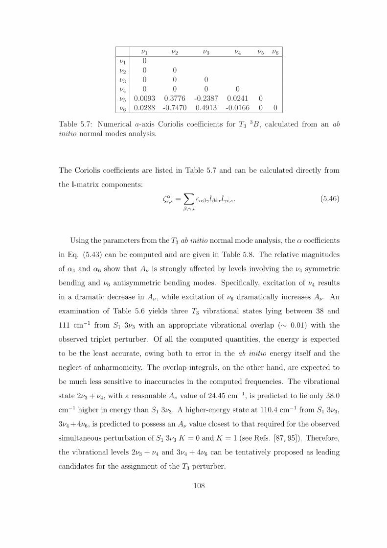
ν1 ν2 ν3 ν4 ν5 ν6
ν1 0ν2 0 0ν3 0 0 0ν4 0 0 0 0ν5 0.0093 0.3776 -0.2387 0.0241 0ν6 0.0288 -0.7470 0.4913 -0.0166 0 0
Table 5.7: Numerical a-axis Coriolis coefficients for T33B, calculated from an ab
initio normal modes analysis.
The Coriolis coefficients are listed in Table 5.7 and can be calculated directly from
the l-matrix components:
ζαr,s =
∑
β,γ,i
εαβγlβi,rlγi,s. (5.46)
Using the parameters from the T3 ab initio normal mode analysis, the α coefficients
in Eq. (5.43) can be computed and are given in Table 5.8. The relative magnitudes
of α4 and α6 show that Aν is strongly affected by levels involving the ν4 symmetric
bending and ν6 antisymmetric bending modes. Specifically, excitation of ν4 results
in a dramatic decrease in Aν , while excitation of ν6 dramatically increases Aν . An
examination of Table 5.6 yields three T3 vibrational states lying between 38 and
111 cm−1 from S1 3ν3 with an appropriate vibrational overlap (∼ 0.01) with the
observed triplet perturber. Of all the computed quantities, the energy is expected
to be the least accurate, owing both to error in the ab initio energy itself and the
neglect of anharmonicity. The overlap integrals, on the other hand, are expected to
be much less sensitive to inaccuracies in the computed frequencies. The vibrational
state 2ν3 + ν4, with a reasonable Aν value of 24.45 cm−1, is predicted to lie only 38.0
cm−1 higher in energy than S1 3ν3. A higher-energy state at 110.4 cm−1 from S1 3ν3,
3ν4 +4ν6, is predicted to possess an Aν value closest to that required for the observed
simultaneous perturbation of S1 3ν3 K = 0 and K = 1 (see Refs. [87, 95]). Therefore,
the vibrational levels 2ν3 + ν4 and 3ν4 + 4ν6 can be tentatively proposed as leading
candidates for the assignment of the T3 perturber.
108
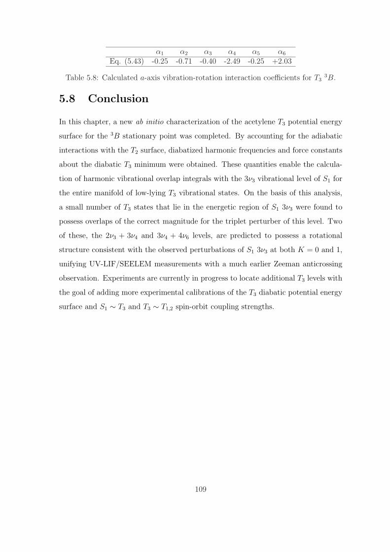
α1 α2 α3 α4 α5 α6
Eq. (5.43) -0.25 -0.71 -0.40 -2.49 -0.25 +2.03
Table 5.8: Calculated a-axis vibration-rotation interaction coefficients for T33B.
5.8 Conclusion
In this chapter, a new ab initio characterization of the acetylene T3 potential energy
surface for the 3B stationary point was completed. By accounting for the adiabatic
interactions with the T2 surface, diabatized harmonic frequencies and force constants
about the diabatic T3 minimum were obtained. These quantities enable the calcula-
tion of harmonic vibrational overlap integrals with the 3ν3 vibrational level of S1 for
the entire manifold of low-lying T3 vibrational states. On the basis of this analysis,
a small number of T3 states that lie in the energetic region of S1 3ν3 were found to
possess overlaps of the correct magnitude for the triplet perturber of this level. Two
of these, the 2ν3 + 3ν4 and 3ν4 + 4ν6 levels, are predicted to possess a rotational
structure consistent with the observed perturbations of S1 3ν3 at both K = 0 and 1,
unifying UV-LIF/SEELEM measurements with a much earlier Zeeman anticrossing
observation. Experiments are currently in progress to locate additional T3 levels with
the goal of adding more experimental calibrations of the T3 diabatic potential energy
surface and S1 ∼ T3 and T3 ∼ T1,2 spin-orbit coupling strengths.
109

110
Chapter 6
Computational Techniques for
Electron-Molecule Scattering
This chapter presents a first and early attempt to formulate a new ab initio electron-
molecule scattering theory relevant to molecular Rydberg states. The majority of the
work in this chapter resulted from a collaboration with Dr. Serhan N. Altunata, and
certain sections were published in an article in the Journal of Chemical Physics [114].
6.1 Introduction
Molecular Rydberg states, in which one electron has been excited into a large-radius
hydrogenic-like orbital, possess several unique properties compared to conventional
ground state molecules. When an electron has been excited into an orbital with a
large mean radius, the electron can be considered to be moving independently of the
non-point charge nature of the molecular ion core. Consequently, the electron-ionic
core system has the general character of a hydrogenic system where an uncorrelated
Rydberg electron only experiences the positive charge of the core (Figure 6-1 (a)).
Accordingly, the energy of the electron-ionic core system follows the Rydberg formula
and can be expressed as a sum of two terms:
E(ν+, N+, n, l, ml
)= I
(ν+, N+
)− RH
(n− µl)2 , (6.1)
111
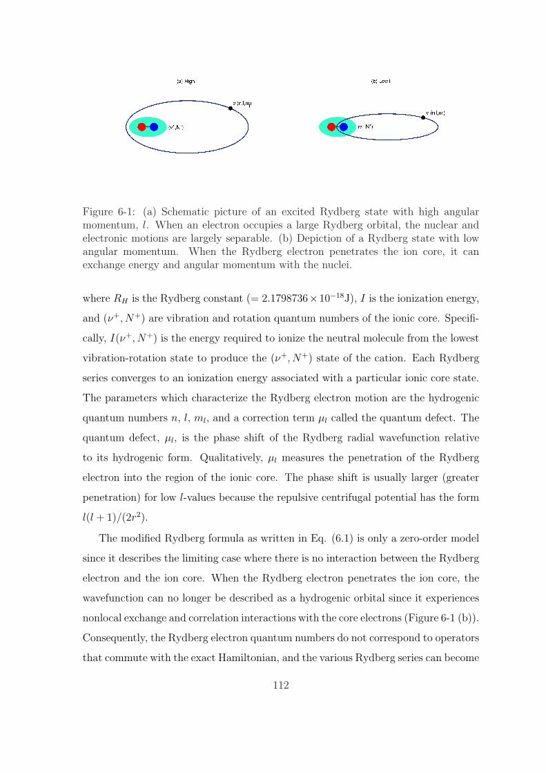
Figure 6-1: (a) Schematic picture of an excited Rydberg state with high angularmomentum, l. When an electron occupies a large Rydberg orbital, the nuclear andelectronic motions are largely separable. (b) Depiction of a Rydberg state with lowangular momentum. When the Rydberg electron penetrates the ion core, it canexchange energy and angular momentum with the nuclei.
where RH is the Rydberg constant (= 2.1798736×10⁻¹⁸J), I is the ionization energy,
and (ν+, N+) are vibration and rotation quantum numbers of the ionic core. Specifi-
cally, I(ν+, N+) is the energy required to ionize the neutral molecule from the lowest
vibration-rotation state to produce the (ν+, N+) state of the cation. Each Rydberg
series converges to an ionization energy associated with a particular ionic core state.
The parameters which characterize the Rydberg electron motion are the hydrogenic
quantum numbers n, l, ml, and a correction term µl called the quantum defect. The
quantum defect, µl, is the phase shift of the Rydberg radial wavefunction relative
to its hydrogenic form. Qualitatively, µl measures the penetration of the Rydberg
electron into the region of the ionic core. The phase shift is usually larger (greater
penetration) for low l-values because the repulsive centrifugal potential has the form
l(l + 1)/(2r2).
The modified Rydberg formula as written in Eq. (6.1) is only a zero-order model
since it describes the limiting case where there is no interaction between the Rydberg
electron and the ion core. When the Rydberg electron penetrates the ion core, the
wavefunction can no longer be described as a hydrogenic orbital since it experiences
nonlocal exchange and correlation interactions with the core electrons (Figure 6-1 (b)).
Consequently, the Rydberg electron quantum numbers do not correspond to operators
that commute with the exact Hamiltonian, and the various Rydberg series can become
112

Figure 6-2: Schematic diagram of a molecule enclosed by a notional sphere of radiusR. Exchange between the scattered and atomic electrons is only important withinthe sphere. The bound wavefunctions centered on nuclei ZA and ZB (only two nucleiare shown for clarity) have negligible amplitude outside the sphere.
mixed. This mixing of Rydberg series can be associated with the semiclassical picture
of a Rydberg electron following a classical trajectory into the core region, exchanging
energy and angular momentum, and emerging with different quantum numbers while
simultaneously causing a change in the core quantum numbers. Rigorously describing
this inelastic process in a quantum mechanical scattering framework is the principal
task of multichannel quantum defect theory (MQDT).
The scattering formalism of MQDT was originally introduced by Seaton [115, 116]
and was extended for molecular systems by Fano [117], Jungen [118], and Greene [119].
Quantum defect theory begins with the simple idea that each Rydberg series and its
associated ionization continuum forms a single “channel” labeled by the quantum
numbers of the Rydberg electron and the ion core. In other words, a channel de-
scribes an initial or final state of the scattering process. In contrast to calculations of
bound-state wavefunctions, MQDT methods partition the configuration space of the
scattering electron into two regions separated by a notional spherical boundary with
radius r = R. An illustration of the division of configuration space is shown in Figure
6-2. The sphere is centered at the center of mass of the molecular target. The radius,
R, of this sphere is chosen large enough to approximately enclose the molecular charge
cloud. In the internal region, r < R, electron exchange and inter-electron correlation
are significant, and the combination of the target molecule and the scattered electron
113

acts similarly to a bound state. Conversely, in the external region, r > R, electron
exchange is negligible, and the scattered electron moves in the coulombic potential
of the target molecule. Specifically, the long range radial solution for the scattered
electron must satisfy the differential equation:
[−1
2
d2
dr2+
l (l + 1)
2r2− Z
r+ V (r)
]ψ (r) =
k2
2ψ (r) , r > R, (6.2)
where the energy E = k2/2 is specified in advance, and V may include higher mul-
tipolar terms present in some problems. For arbitrary positive or negative energy,
quantum defect theory is based on the analytical properties of the regular and irregu-
lar solutions of Eq. (6.2), denoted by f(k, r) and g(k, r) respectively. These scattering
or continuum functions are centered about the center of mass of the molecular target
and must have significant amplitude on the spherical boundary. Their presence ac-
counts for the escape of the scattered electron to the external region and yields the
correct asymptotic behavior of the collision wavefunctions. The general wavefunction
can therefore be expressed by the superposition of f(k, r) and g(k, r) in terms of the
scattering reaction matrix K [120]:
Ψ =∑
j
Y (j)∑
i
|i〉 [fi (k, r) δij − gi (k, r) Kij], (6.3)
where i and j represent particular channels, and Y (j) is the wavefunction of the ion
core multiplied by the angular parts of the Rydberg electron wavefunction. The
off-diagonal matrix elements of K represent the strength of the mixing between the
various channels. As shown by Seaton [115, 116], one can define the matrix
µij =1
πtan−1(Kij), (6.4)
where µij are the elements of the quantum defect matrix. The matrix elements µij are
the multichannel analogue of the one-dimensional quantum defect in Eq. (6.1). It is
important to point out that the K matrix is valid both below and above any ionization
threshold, and the MQDT treatment is able to treat both ionization continua and
114
bound Rydberg states within a single formalism.
The following sections outline a recent and an early attempt to derive and calcu-
late a multi-electron reaction matrix, K, based on a variational formalism. It is not
the intent of this chapter to give an exhaustive review of the derivation or to include
the numerous calculations which have been carried out with this method. Such infor-
mation can be found in Refs. [114, 121] and also in Appendix C. The purpose of this
chapter is to provide a pedagogical exposition of the technical aspects of the method,
and the expert reader should refer to Chapter 6 of Ref. [121] for a complete deriva-
tion of the multi-electron K matrix. This chapter concludes with the calculation of
the single channel reaction matrix for the 1sσg4pσu1Σ+
u Rydberg state of H2 as an
example and first test of the theory.
6.2 Variational Derivation of the K matrix
The basic concept of the multichannel K matrix theory derived in Ref. [121] is most
easily illustrated by the simple one channel scattering of a spinless particle by a
spherically symmetric potential V (r). Only the one channel situation is considered
in this chapter since this significantly simplifies the derivation and notation of Ref.
[121]; furthermore, the more technical aspects of the multichannel case are already
explained in Ref. [121], so presenting the full theoretical details would be unnecessary.
All of the derivations in this section are presented to give a clear explanation and to
highlight the analogies with the multichannel case.
The single channel radial Schrodinger equation in atomic units can be written as
Lu (r) = 0, (6.5)
with
L = −1
2
d2
dr2+ V (r)− k2
2, (6.6)
where limr→∞
V (r) = 0 and the energy E = k2/2. From the definition of L one can
115

define the function L:
L =
∫ ∞
0
u∗ (r) Lu (r) dr. (6.7)
The boundary conditions assumed for u(r) are
u (0) = 0, (6.8)
limr→∞
u (r) = f (kr) + Kg (kr) , (6.9)
where f and g are two linearly independent solutions of the radial Schrodinger equa-
tion, and the coefficient of the latter is the K matrix which is just a 1× 1 matrix in
this one channel case.
When u(r) is an exact solution of the radial Schrodinger equation, the functional Lvanishes. The change in the functional L as the exact u(r) is varied can be examined
by replacing u(r) by a trial solution, ut(r), satisfying the same boundary conditions
specified by Eqs. (6.8)–(6.9). Specifically, ut(r) is defined by
δu (r) = ut (r)− u (r) , (6.10)
with the boundary conditions
δu (0) = 0, (6.11)
limr→∞
δu (r) = δKg (kr) . (6.12)
Carrying out the variation of L gives
δL =
∫ ∞
0
[u∗ (r) + δu∗ (r)] L [u (r) + δu (r)] dr
=
∫ ∞
0
u∗ (r) Lδu (r) dr +
∫ ∞
0
δu∗ (r) Lδu (r) dr.
(6.13)
where the last step follows from the definition that u(r) is an exact solution to the
Schrodinger equation, Lu(r) = 0. The first term in Eq. (6.13) can be expanded by
using integration by parts twice:
116
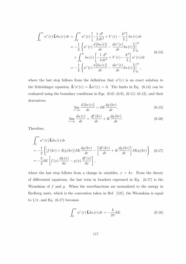
∫ ∞
0
u∗ (r) Lδu (r) dr =
∫ ∞
0
u∗ (r)
[−1
2
d2
dr2+ V (r)− k2
2
]δu (r) dr
= −1
2
u∗ (r)
d [δu (r)]
dr− du∗ (r)
drδu (r)
∣∣∣∣∞
0
+
∫ ∞
0
δu (r)
[−1
2
d2
dr2+ V (r)− k2
2
]u∗ (r) dr
= −1
2
u∗ (r)
d [δu (r)]
dr− du∗ (r)
drδu (r)
∣∣∣∣∞
0
,
(6.14)
where the last step follows from the definition that u∗(r) is an exact solution to
the Schrodinger equation, L∗u∗(r) = Lu∗(r) = 0. The limits in Eq. (6.14) can be
evaluated using the boundary conditions in Eqs. (6.8)–(6.9), (6.11)–(6.12), and their
derivatives:
limr→∞
d [δu (r)]
dr= δK
dg (kr)
dr, (6.15)
limr→∞
du (r)
dr=
df (kr)
dr+ K
dg (kr)
dr. (6.16)
Therefore,
∫ ∞
0
u∗ (r) Lδu (r) dr
= −1
2
[f (kr) + Kg (kr)] δK
dg (kr)
dr−
[df (kr)
dr+ K
dg (kr)
dr
]δKg (kr)
= −k
2δK
[f (x)
dg (x)
dx− g (x)
df (x)
dx
],
(6.17)
where the last step follows from a change in variables, x = kr. From the theory
of differential equations, the last term in brackets expressed in Eq. (6.17) is the
Wronskian of f and g. When the wavefunctions are normalized to the energy in
Rydberg units, which is the convention taken in Ref. [121], the Wronskian is equal
to 1/π, and Eq. (6.17) becomes
∫ ∞
0
u∗ (r) Lδu (r) dr = − k
2πδK. (6.18)
117

Substituting Eq. (6.18) in Eq. (6.13) gives
δL = − k
2πδK +
∫ ∞
0
δu∗ (r) Lδu (r) dr. (6.19)
Eq. (6.19) expresses the exact value of K in terms of the approximate value of
the functional L and a term which is second order in the error in the wavefunction.
Setting δL = 0 and substituting Eq. (6.10) in Eq. (6.19) gives
K = Kt +2π
k
∫ ∞
0
u∗t (r) Lut (r) dr, (6.20)
where the label “t” refers to a trial state or matrix. Eq. (6.20) can be solved explicitly
for a trial wavefunction that contains the linear trial coefficients ci. The strategy is
to choose a trial function of the form
ut (r) = f (k, r) + Kg (k, r) +n∑
i=1
ciφi (r), (6.21)
where φi(r) are a set of unspecified, real, square-integrable energy independent
basis functions. In order to keep the same notation as the work presented in Ref.
[121], Eq. (6.21) can be expressed more compactly by relabeling the basis functions
f(k, r), g(k, r), and φi(r) into a single set φi(r), i = 0, . . . , n + 1 with φ0 = f(k, r),
φ1 = g(k, r), and c1 = K. Using this convention, Eq. (6.21) becomes
ut (r) = φ0 (r) +n+1∑i=1
ciφi (r), (6.22)
Substituting ut(r) into the variational expression of Eq. (6.20) gives (after some
manipulation):
K =2π
k
[∫ ∞
0
φ∗0 (r) Lφ0 (r) dr+n+1∑i=1
c∗i
∫ ∞
0
φ∗i (r) Lφ0 (r) dr
+n+1∑i=1
ci
∫ ∞
0
φ∗0 (r) Lφi (r) dr +n+1∑i,j=1
c∗i cj
∫ ∞
0
φ∗i (r) Lφj (r) dr
] (6.23)
118
or in matrix notation
K =2π
k
(m00 + c†m0 + m0
†c + c†mc), (6.24)
with
m00 =
∫ ∞
0
φ∗0 (r) Lφ0 (r) dr, (6.25)
(m0)i =
∫ ∞
0
φ∗i (r) Lφ0 (r) dr, (6.26)
(m)ij =
∫ ∞
0
φ∗i (r) Lφj (r) dr, (6.27)
and c is a column vector of the n + 1 linear trial coefficients ci. Eqs. (6.25)–(6.27)
define the free-free 1 × 1 matrix m00, the bound-free N × 1 matrix m0, and the
bound-bound N × N matrix m. An optimization of Eq. (6.24) with respect to the
expansion coefficients c is determined from the condition:
∂K
∂ci
= 0, i = 1, . . . , n + 1, (6.28)
The result of this condition on Eq. (6.24) gives
c = −m−1m0, (6.29)
Substituting this result into Eq. (6.24) finally yields
K =2π
k
[m00 +
(−m−1m0
)†m0 + m0
† (−m−1m0
)
+(−m−1m0
)†m
(−m−1m0
)]
=2π
k
(m00 −m0
†m−1m0
).
(6.30)
This single channel equation is completely analogous to the generalized multi-
channel K matrix expression in Eq. (6.2.73) of Ref. [121] which is given by
Kvar = 2πB0−1
(m00 −m10
†m11−1m10
)B0
−1. (6.31)
119
The additional matrix B0 in the multichannel case arises from the normalization of
the f(k, r) and g(k, r) functions with the ion core molecular basis. In the multichannel
case, the matrices m00, m10, and m11 are no longer integrals between one-electron
functions; instead they represent an integration between antisymmetrized products
of bound N -electron ion core orbitals, Θ, and the free scattered electron, φ0 or φ1.
For example, the elements of m00 are defined as
(m00)pq =
∫
r1···rN+1<R
A
[Θ∗
pφ∗0,p
]L A [Θqφ0,q] dr1 · · · drN+1, (6.32)
where the multidimensional integration is always confined within the spherical volume
of radius R (cf. Figure 6-2). In Eq. (6.32), A is the antisymmetrizing operator, and
the indices p and q represent all the quantum numbers needed to represent the internal
state of the ion core target. The matrices m10 and m11 are defined similarly.
6.3 Numerical Evaluation of Integrals
The variational form of the K matrix is reduced to the evaluation of matrix elements
that can be classified as either free-free, bound-free, or bound-bound, depending on
whether two, one, or zero scattering basis functions appear in the integrals. However,
since the integration is carried out over the finite volume of the K matrix sphere, the
computation of the one- and two-electron integrals is significantly more difficult than
their infinite-volume counterparts. Slater-type orbitals have been used in previous
work [122, 123] for atomic and diatomic systems, but their applicability to general
scattering problems incurs the enormous computational cost of numerical evaluation
of Hamiltonian matrix elements. For polyatomic molecular systems, several atom-
centered basis functions must be used, and the computation becomes prohibitively
time consuming if numerical algorithms are implemented. Consequently, Cartesian
Gaussian-type functions and linear combinations of Gaussians have become widely
used as bound state basis set orbitals in molecular scattering theory [124]. Although
it is relatively easy to describe the bound state target orbitals with Gaussian-type
120

functions, the choice of the continuum basis set is more difficult. The continuum basis
must be a good approximation to the f(k, r) and g(k, r) functions, which are both
oscillatory and have significant amplitude on the K matrix sphere. Fortunately, a
basis set of orthogonal continuum functions can be replaced by a fit to several diffuse
Gaussian-type functions (described further in the following section). This approach
reduces the problem of multidimensional numerical integration to a sum of Gaussian
integrals; however, the remaining complication is the non-trivial computation of the
individual matrix elements over a finite volume. These matrix elements, or integrals,
must be evaluated accurately and efficiently in order to obtain reliable theoretical
predictions for ab initio calculations of generic molecular systems.
It should be mentioned that the efficient evaluation of molecular integrals for
bound-state calculations has been a topic of many studies for as long as 50 years [125,
126, 127, 128, 129]. Most notably, the high efficiency of the Head-Gordon and Pople
algorithm has allowed current programs to evaluate two-electron integrals dynamically
in computer memory as needed [130]. To capitalize on the high efficiency of these
algorithms, the most practical modification needed to incorporate existing electronic
structure programs into the K matrix calculation is to subtract the contribution from
the outer region of the K matrix sphere from the integrals calculated over all space.
In the present work, the PSI 3.2.2 software package was used to generate the integrals
over all space for up to k-type (l = 9) angular momentum basis sets [131]. Since it
is assumed that the bound target basis functions have negligible amplitude outside
the K matrix sphere, the only matrix elements which need to be modified in the
PSI 3.2.2 output are those integrations involving two or more continuum orbitals.
Morgan, Gillan, Tennyson, and Chen have briefly discussed how one might proceed
to evaluate the continuum integrations in Ref. [124], but they did not present a full
derivation. Closed form analytic expressions for the one- and two-electron integrals of
Cartesian Gaussian orbitals outside the K matrix sphere are given in Ref. [114] and
Appendix C. These integrals, which are (cutely) called “tail integrals,” are evaluated
as finite summations over standard functions; hence, the results are accurate within
computer precision.
121
6.4 Representing the Continuum Functions
With the completion of an efficient and accurate integral program, all of the necessary
routines to calculate the K matrix can be carried out on a computer. The calculation
commences with the computation of occupied and virtual orbitals of the target ion
using standard quantum chemistry techniques. During early testing of the present
work, it was sufficient to use a single Hartree Fock configuration representation of
the lowest electronic state of the molecule. The self consistent field program from the
PSI 3.2.2 suite solves the Hartree Fock procedure and provides the orbital expansion
coefficients. Next, a customized routine solves the differential equation in Eq. (6.2)
for the numerical continuum basis functions fl(k, r) and gl(k, r) with the energy E =
k2/2, and angular momentum l specified in advance by the user. Each of the radial
continuum basis functions are then fit to a linear combination of Gaussians of the
form∑
i
cirl exp
(−αir2). (6.33)
Since each of the continuum basis functions is a solution to the partial wave dif-
ferential equation (cf. Eq. (6.2)), the angular momentum quantum number l, by
definition, is conserved. Consequently, both fl(k, r) and gl(k, r) must be fit to Gaus-
sians all sharing the same center, which is usually taken as the center of mass of the
molecule. In this way, each of the Gaussians which comprise the linear combination
can be multiplied by the same spherical harmonic in order for the entire expansion
to still be an eigenfunction of L. Fitting the radial continuum basis functions by
a set of Gaussians is extremely difficult since one must represent a large number of
nodes with nodeless Gaussian functions expanded about a single center (see Figures
6-3 (a)–(b)). The procedure used to obtain the Gaussian exponents was performed
by numerically minimizing the function
Fl (α1, . . . , αn) =∑
k
[n∑i
cirlk exp
(−αir2k
)− φl (rk)
]2
. (6.34)
The radial coordinate rk spans a dense grid of points over which the continuum
122

Figure 6-3: (a)–(b) Analytical continuum functions fl(k, r) and(1− e−λrl+1
)gl(k, r)
with l = 1 (crosses). Each of the continuum functions are fit by a linear combinationof 9 single-centered Gaussian functions (full curves) for E = −0.03125 Hartrees.
function φl (= fl(r, k) or gl(r, k)) is to be fitted. This minimization is highly nonlinear
and makes the final fit very sensitive to the initial guess of exponents. In the present
work, it was empirically found that a geometric series of the form [132]
αi = 0.016× 1.39i, i = 1, 2, 3, . . . , n, (6.35)
was found to provide initial guesses which significantly minimized computer time
for both fl(k, r) and gl(k, r). Using these starting exponents, the coefficients ci are
determined by an automated least squares fit to φl using the grid points rk. Next,
the minimum of Fl (α1, . . . , αn), using the n αi as variational parameters, is obtained
using a Powell dogleg algorithm very similar to the methods described in Chapter
2. After this procedure is carried out, the coefficients ci are updated by fitting to φl
using the new exponents. The Powell dogleg method to update the αi exponents is
then repeated using the new coefficients ci and old αi exponents as initial guesses.
The cyclic process of using the least squares fit for ci and the Powell dogleg method
for αi is repeated until convergence is reached.
The quality of the Gaussian basis sets for representing fl(k, r) and gl(k, r) each
with l = 1 and energy E = −0.03125 Hartrees can be seen in Figures 6-3 (a)–(b). The
gl(k, r) function, which must be regular at r = 0 for a practical numerical implementa-
tion, is multiplied by the cut-off function(1− e−λrl+1
)which removes the singularity
123

fl(k, r) fl(k, r)(1− e−λrl+1
)gl(k, r)
(1− e−λrl+1
)gl(k, r)
i αi exponents ci coefficients αi exponents ci coefficients1 0.015982 0.32159 0.021174 -1.572932 0.024189 -2.83213 0.029195 8.055893 0.033825 9.04025 0.040072 -20.382744 0.046443 -17.42405 0.054798 35.546475 0.063458 24.42726 0.074561 -47.011956 0.086156 -25.62546 0.100944 48.256377 0.116873 19.94605 0.136341 -37.512218 0.158115 -10.25389 0.184532 20.046719 0.217796 2.74745 0.254361 -5.99542
Table 6.1: Optimized Gaussian exponents and coefficients for representing continuumfunctions with l = 1 and E = −0.03125 Hartrees. All exponents, αi, are in units ofBohr−2.
at the origin and approaches unity for large r. The curves labeled with crosses rep-
resent the actual continuum functions, and the full curves are their approximations
by a linear combination of 9 single center Gaussians. Table 6.1 gives the Gaussian
exponents αi and coefficients ci for the fits to the continuum functions. From the
figures, the difference between the continuum functions and their approximations is
hardly noticeable.
6.5 Additional Computational Details
After a numerical fit representing the continuum bases is achieved, the spherical
harmonic Gaussians in Eq. (6.33) are converted to their Cartesian Gaussian coun-
terparts using Eq. (C.36) in Appendix C. This additional step is necessary since all
the one- and two-electron “tail integrals” are most easily computed in a Cartesian
Gaussian basis. It is important to note at this point that all the bound and con-
tinuum functions should be constructed to be orthogonal since this greatly simplifies
the evaluation of the Hamiltonian matrix elements. Therefore, a customized module
reads a set of bound molecular orbital expansion coefficients, a pair of continuum
functions, and generates an orthogonal orbital set using a Schmidt orthogonalization
procedure. This results in the continuum orbitals picking up bound orbital compo-
124

nents – a feature that can cause practical linear dependence problems at the four
index transformation stage if the coefficients produced are large [133].
Next, all the one- and two-electron integrals for the scattering calculation are gen-
erated using a highly vectorized code which evaluates the “tail integral” expressions in
Appendix C. The most computationally expensive step in the scattering calculation
is the evaluation of the two-electron integrals:
〈ij|kl〉 =
∫ ∫χ∗i (r1) χj (r1)
1
|r1 − r2|χ∗k (r2) χl (r2) dr1dr2. (6.36)
As written, the computation of the two-electron matrix elements would require n4
six-dimensional integrals, where n is the number of atomic centered functions. This
is exceedingly expensive in terms of computer time even for small molecules. Since all
of the orbitals are real (this is only true for ml = 0 scattering states, which is the only
case studied in the next section), the complex conjugation has no effect, and orbitals
i and j or k and l can be interchanged to obtain the same integral. Furthermore, the
orbitals associated with electron 1 can be swapped with those associated with electron
2. Therefore, the two-electron integrals have approximately eightfold symmetry:
〈ij|kl〉 = 〈ji|kl〉= 〈ij|lk〉= 〈ji|lk〉= 〈kl|ij〉= 〈lk|ij〉= 〈kl|ji〉= 〈lk|ji〉 .
(6.37)
The approximately eightfold symmetry saves significant computer time since only
about one in eight of the two-electron integrals are unique and must be computed (the
exact number of unique two-electron integrals is actually n (n + 1) (2 + n (n + 1)) /8).
Once these atomic integrals are available, a four index transformation program
125

multiplies them by combinations of molecular orbital coefficients:
〈st|uv〉 =∑
i,j,k,l
ciscjt 〈ij|kl〉 ckuclv, (6.38)
where cjt are the atomic function coefficients, i, j, k, l are atomic centered functions,
and s, t, u, v are molecular orbitals. The two-electron integral transformation as
written in Eq. (6.38) requires n8 arithmetic operations where n is the number of
atomic centered functions. Using the summation restructuring scheme of Yoshimine
[134], the integral transformation was reduced to n5 arithmetic operations in the
current codes. After this computationally expensive step, another module generates
configuration state functions with the appropriate spin and symmetries for the system
under study. Finally, the Hamiltonian matrix elements are evaluated, and the m00,
m10, and m11 matrices are formed to complete the calculation of the K matrix.
6.6 Test Calculations on the 1sσg4pσu1Σ+
u State of
H2
As a simple and first test of the variational K matrix theory, calculations were carried
out on the 1sσg4pσu1Σ+
u Rydberg state for the two-electron H2 molecule. Only a
single channel was included in the calculation, and the one-electron ion core was
approximated as a single Slater determinant. Accordingly, the ion core was calculated
at the restricted open shell Hartree Fock (ROHF) level with the standard 6-31G basis
set [135]. All bound type configurations (φi in Eq. (6.21)) were obtained by placing an
additional electron in the lowest three σu virtual orbitals of the ion core. In this way,
configurations of the form 1sσgnpσu were generated to finally construct an overall
state with 1Σu symmetry.
Next, the two-electron reaction matrix K was generated as a function of energy
by calculating the m00, m10, and m11 matrices over a grid of energy points. Using
the definition in Eq. (6.4), the quantum defects were produced from the K matrix
and subsequently used in Eq. (6.1) to determine the potential energy curve for the
126

Figure 6-4: Potential energy curves for the H+2 ion ground state and the 1sσg4pσu
1Σ+u state of H2. Energies for the H+
2 ion were calculated at the ROHF level withthe 6-31G basis, and the solid energy curve is the result of a high level ab initiocalculation by Staszewska et al. [2]. The blue data points were obtained from thetwo-electron K matrix calculation described in this work.
1sσg4pσu1Σ+
u electronic state of H2. In Figure 6-4, the results of this work are
compared to the high level calculation reported by Staszewska et al. in Ref. [2]. Good
agreement between this work and the previous high-level calculation is observed in
the vicinity of the equilibrium internuclear distance; however, the deviations become
more significant at larger internuclear distances. It seems reasonable to expect these
deviations since the ROHF wavefunction is a poor approximation for large electronic
distances [135].
It should be mentioned at this point that additional test calculations on H2 were
subsequently performed using basis sets of triple zeta quality. These larger basis sets
generate more σu virtual orbitals of the ion core which must be orthogonalized to
the continuum functions. Consequently, severe problems of linear dependence were
encountered due to the increased number of target wavefunctions which must be
orthogonalized to the continuum basis. Several authors have also reported serious
problems with linear dependence for electron collisions with polyatomic molecules
[133, 136, 137, 138, 139, 140, 141]. It may be possible to use the results of the
Schmidt procedure to remove functions from the basis, but tests with the existing
codes showed that this did not work well. Until this complicated issue is addressed in
the current methods, one cannot be completely definitive about the simple calculation
127
presented in Figure 6-4 (or even possibly, the methodology involved). Nevertheless,
the approaches described in this chapter and in Ref. [121] are a useful guide for future
calculations aimed at incorporating scattering theories with conventional bound state
methods.
6.7 Conclusion
This chapter has described a large and complex software package which was initially
used to carry out ab initio calculations on electron scattering by molecular targets.
All of the programs in this package were based on a variational determination of
the K matrix which embodies the information on the scattering process. The most
computationally intensive step in the scattering calculation is the computation of
coulomb and exchange integrals within a finite spherical volume. Rather than modify
highly efficient codes for molecular integral evaluation, subtracting the outer or tail
regions permits the evaluation of Hamiltonian matrix elements within the required
finite spherical volume. Thus, the implementation of the current approach, exploiting
current bound-state software packages, is straightforward and practical. Furthermore,
the proposed scheme of using single center Gaussian functions to represent the con-
tinuum electron fits conveniently within the framework developed in this work. A
detailed numerical analysis of the nonlinear fit to Gaussians and the final compu-
tation of the K matrix for the 1sσg4pσu1Σ+
u state of H2 provide a first test of the
approximations and expressions.
Inherent in all computer packages of this type is the need to extend it to larger
and more complicated molecular targets. However, difficulties in further development
of this program suite arise due to linear dependence problems between the target and
continuum wavefunctions. As discussed in the previous sections, the use of larger
basis sets for the ion target lead to significant overlap with the continuum functions,
resulting in noninvertible overlap matrices or unusually large coefficients at the four
index transformation stage. This is not surprising since single-centered continuum
functions are a fairly crude approximation for molecules possessing anisotropic po-
128

tentials (such as large dipoles or polar polyatomic targets). Numerically solving for
the continuum functions directly (as opposed to a nonlinear fit and subsequent or-
thogonalization) from a multi-electron potential may solve the current difficulties.
The use of finite element numerical functions to represent the continuum for polar
molecules is an ongoing work and the subject of the next chapter.
129

130

Chapter 7
Developments in Electron
Scattering for Polar Molecules
This chapter outlines preliminary work on an electron-molecule scattering approach
for Rydberg states of highly polar diatomics. The majority of the work presented in
this chapter is currently in progress and still in development.
7.1 Introduction
Electronic structure calculations to determine excited state potential energy curves
for heavy atom systems are difficult. Due to the large number of inner shell electrons
which can give rise to numerous interactions, applying the standard quantum chem-
istry methods to these systems is sometimes not feasible. As discussed in the previous
chapter, the tools of conventional quantum chemistry mostly rely on variational ap-
proaches that minimize variables (usually the total energy) subject to constraints,
and therefore generalize poorly to highly excited states. Not surprisingly, it is only
within the last twenty years that techniques for excited state calculations have begun
to achieve the same accuracy as their ground state counterparts [142, 143, 144, 145].
Unfortunately, this type of accuracy usually comes with great computational expense.
One of the many examples where ab initio calculations have progressed slowly is
the prediction of the electronic spectrum for the alkaline earth halides. The alkaline
131
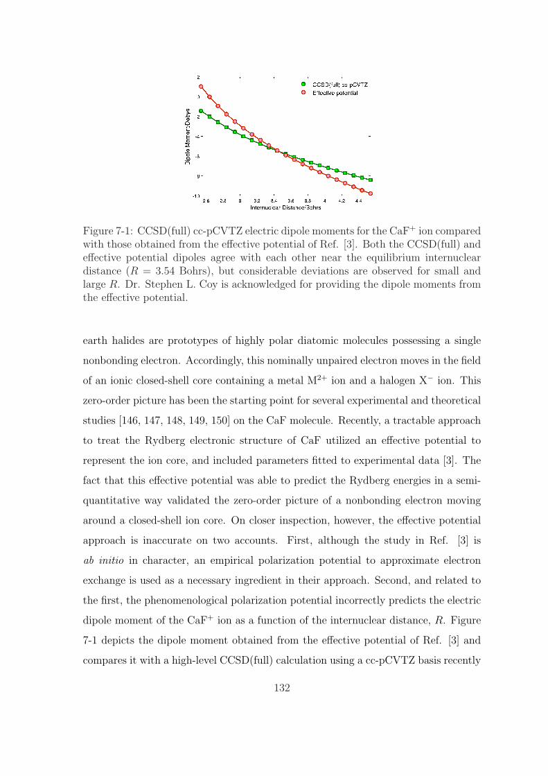
Figure 7-1: CCSD(full) cc-pCVTZ electric dipole moments for the CaF+ ion comparedwith those obtained from the effective potential of Ref. [3]. Both the CCSD(full) andeffective potential dipoles agree with each other near the equilibrium internucleardistance (R = 3.54 Bohrs), but considerable deviations are observed for small andlarge R. Dr. Stephen L. Coy is acknowledged for providing the dipole moments fromthe effective potential.
earth halides are prototypes of highly polar diatomic molecules possessing a single
nonbonding electron. Accordingly, this nominally unpaired electron moves in the field
of an ionic closed-shell core containing a metal M2+ ion and a halogen X− ion. This
zero-order picture has been the starting point for several experimental and theoretical
studies [146, 147, 148, 149, 150] on the CaF molecule. Recently, a tractable approach
to treat the Rydberg electronic structure of CaF utilized an effective potential to
represent the ion core, and included parameters fitted to experimental data [3]. The
fact that this effective potential was able to predict the Rydberg energies in a semi-
quantitative way validated the zero-order picture of a nonbonding electron moving
around a closed-shell ion core. On closer inspection, however, the effective potential
approach is inaccurate on two accounts. First, although the study in Ref. [3] is
ab initio in character, an empirical polarization potential to approximate electron
exchange is used as a necessary ingredient in their approach. Second, and related to
the first, the phenomenological polarization potential incorrectly predicts the electric
dipole moment of the CaF+ ion as a function of the internuclear distance, R. Figure
7-1 depicts the dipole moment obtained from the effective potential of Ref. [3] and
compares it with a high-level CCSD(full) calculation using a cc-pCVTZ basis recently
132
published for the Ca atom [151]. An inspection of the dipole moment reveals that
the effective potential is not quantitatively accurate in the small or large R limit.
The natural solution to this problem is to re-solve the MQDT equations using
a multi-electron ab initio approach. By invoking the rigorous methods of quantum
chemical techniques, it is possible to fix the incorrect dipole dependence on internu-
clear distance and also eliminate any empirical parameters at the same time. The fol-
lowing sections describe preliminary and ongoing steps to incorporate multi-electron
methods within an MQDT approach.
7.2 The Electron Scattering Equations
The full Hamiltonian for the scattering of an electron by a non-rotating diatomic
molecule is given by
H = Hion (r1, . . . , rN−1) + Vint (r1, . . . , rN)− 1
2∇2
rN. (7.1)
where the scattered electron is denoted by the subscript N , and the diatomic ion has
N − 1 electrons with positions ri and 2 nuclei with positions Ri and charge Zi:
Hion = −1
2
N−1∑i=1
∇2ri− 1
2
2∑i=1
∇2Ri−
N−1∑i=1
2∑j=1
Zj
|ri −Rj| +2∑
i>j
ZiZj
|Ri −Rj|
+N−1∑i>j
1
|ri − rj| .(7.2)
The term Vint is given by
Vint = −2∑
i=1
Zi
|rN −Ri| +N−1∑i=1
1
|rN − ri| . (7.3)
In the fixed-nuclei approximation, the electronic problem can be treated alone, and
the ion wavefunctions, Φγ (x1, . . . ,xN−1, R), satisfy
(Hion − Eγ
)Φγ (x1, . . . ,xN−1, R) = 0, (7.4)
133
where the x coordinate includes both space and spin, and R is the internuclear dis-
tance. The subscript γ represents the set of quantum numbers that fully describe an
eigenstate of the ion. The total wavefunction Ψ (x1, . . . ,xN , R) can be expanded in
terms of the ion eigenfunctions:
Ψ (x1, . . . ,xN , R) = A∑
γ
Φγ (x1, . . . ,xN−1, R) Fγ (xN), (7.5)
where A is the antisymmetrizing operator and Fγ (xN) is the scattered electron func-
tion. The sum over γ allows different configurations of the target ion and scattered
electron to contribute. When only the ground state wavefunction in this expansion
is retained (which is the only case considered in this chapter), the static exchange
approximation is obtained:
Ψ (x1, . . . ,xN , R) = AΦ (x1, . . . ,xN−1, R) F (xN) . (7.6)
Since only closed shell ions are treated in this chapter, one can reduce Eq. (7.5) further
by assuming the ion wavefunction, Φ (x1, . . . ,xN−1, R), is known in the Hartree-Fock
approximation to be a single determinant:
Φ (x1, . . . ,xN−1, R) =1√
(N − 1)!|U1 (x1) · · ·UN−1 (xN−1)| , (7.7)
where the Ui (x1) are single-electron ion orbital functions. Substituting Eq. (7.7) into
Eq. (7.6) and using the properties of Slater determinants [135], one can show that
F (r) satisfies the integro-differential equation
[−1
2∇2 − 1
2k2 + Vs (r)
]F (r) =
Nocc∑α=1
[∫U∗
α (s)1
|r− s|F (s) ds
]Uα (r) , (7.8)
where the static potential Vs (r) is
Vs (r) =Nocc∑α=1
∫U∗
α (s)1
|r− s|Uα (s) ds +2∑
i=1
Zi
|r−Ri| , (7.9)
134

and1
2k2 = E − E0, (7.10)
with E0 being the ground state energy of the ion.
Eqs. (7.8)–(7.9) treat the evaluation of the scattered electron function within the
framework of the static exchange approximation. Specifically, the local and nonlocal
interactions of the scattered electron with the ion core are included, but correlation is
completely neglected. The neglected correlation terms can be included approximately
by adding a polarization potential to Vs of the form
Vpol = − 1
2r4(α0 + α2P2 (cos θ)) , (7.11)
where α0 and α2 are the totally symmetric and nontotally symmetric components of
the polarizability tensor which can be calculated using ab initio electronic structure
codes. The additional Vpol term approximately accounts for any contribution coming
from the distortion of the ion orbitials due to the perturbative effect of the impinging
electron.
7.3 A Partial Differential Equation Approach
The single-electron ion orbital functions, Uα (r), can be obtained from conventional
electronic structure programs in a basis set of Cartesian Gaussians. On the other
hand, the evaluation of the continuum function F (r) as a function of k in Eq. (7.8) is
more difficult. As discussed in Chapter 6, F (r), oscillates significantly as a function
of radial distance and does not even approach 0 as r → ∞ when the scattered
electron energy exceeds the ionization energy. Consequently, Gaussian-type basis
sets are not well-suited to approximate the free-particle wavefunction F (r) at large
distances. Furthermore, some diatomics have highly polar ionic cores, which imply
that the continuum function F (r) has some multi-center character; therefore, the
nonlinear fits by single-center Gaussians discussed in Chapter 6 are not applicable.
For these reasons, a partial differential equation (PDE) approach adapted to diatomics
135

is currently being used to solve Eq. (7.8). The necessary equations and methods are
described in the present and following sections.
The integro-differential expression in Eq. (7.9) can be implemented in a PDE
solver by rewriting it as
[−1
2∇2 − 1
2k2 + Vs (r)
]F (r) =
Nocc∑α=1
Wα (r) Uα (r), (7.12)
where Wα (r) is the exchange integral
Wα (r) =
∫U∗
α (s)1
|r− s|F (s) ds, α = 1, . . . , Nocc. (7.13)
A useful property to remember is that the Coulomb potential is the Green’s function
of the Laplacian:
∇2r
1
|r− s| = −4πδ (r− s) . (7.14)
Therefore, when Wα (r) is acted upon by the ∇2 operator, one obtains
∇2rWα (r) =
∫U∗
α (s)∇2r
1
|r− s|F (s) ds
=
∫U∗
α (s) [−4πδ (r− s)] F (s) ds
= −4πU∗α (r) F (r) , α = 1, . . . , Nocc.
(7.15)
Thus, Eq. (7.12) combined with Eq. (7.15) is a system of Nocc + 1 coupled, three-
dimensional PDE’s for the scattering function F (r) and the exchange kernels Wα (r).
It is important to note that this set of equations has no integral terms but must be
solved simultaneously. If this PDE approach is confined to diatomic systems, the
cylindrical symmetry can be used to reduce the dimensionality of the PDE system.
For example, Figure 7-2 shows the coordinate system for a CaF+ ion aligned along
the z-axis. The origin of the coordinate system is located at the center of mass of the
CaF+ ion, and the orientation of the diatomic is chosen such that the dipole moment
points towards the positive z-axis. Since m is a good quantum number, the azimuthal
dependence is exactly separable in this coordinate system, and one can write:
136

Figure 7-2: Coordinate system for a CaF+ ion used throughout Chapter 7. The CaF+
ion is aligned along the z-axis with the origin at its center of mass. The orientation ofthe z-axis is defined such that the dipole moment points towards the positive z-axis.
F (m) (r) =f (m) (v)
r√
1− η2
eimφ
√2π
, (7.16)
and
Uα (r) =uα (v)
r√
1− η2
eimαφ
√2π
, (7.17)
where η = cos θ, and the vector v has two components given by v = (r, η). The
azimuthal quantum numbers m and mα are restricted to integer values, i.e., 0 for σ
orbitals, ±1 for π orbitals, ±2 for δ orbitals, etc.
The Laplacian in the (r, η, φ) coordinates is given by
∇2 =1
r2
∂
∂r
(r2 ∂
∂r
)+
1
r2
∂
∂η
[(1− η2
) ∂
∂η
]+
1
r2 (1− η2)
∂2
∂φ2. (7.18)
Substituting this form of the Laplacian in Eq. (7.12) and using the definition in Eq.
(7.17) gives, after significant manipulation,
137

(1
2
[1√
1− η2
∂2
∂r2f (m) (v) +
f (m) (v)
r2 (1− η2)3/2+
√1− η2
r2
∂2
∂η2f (m) (v)
− m2f (m) (v)
r2 (1− η2)3/2
]+
1
2
k2f (m) (v)√1− η2
)eimφ
= V (v)f (m) (v)√
1− η2eimφ −
Nocc∑α=1
W (m)α (r)
uα (v)√1− η2
eimαφ.
(7.19)
Substituting Eqs. (7.16) and (7.17) in Eq. (7.15) gives
∇2rW
(m)α (r) = −2
u∗α (v) f (m) (v)
r2 (1− η2)ei(m−mα)φ, α = 1, . . . , Nocc. (7.20)
One can also use cylindrical symmetry to define the following:
W (m)α (r) =
w(m)α (v)
r√
1− η2ei(m−mα)φ. (7.21)
Substituting this definition in Eqs. (7.19)–(7.20), and after even more manipulation,
one finally obtains
∂2
∂r2
f (m) (v)
1− η2+
(1−m2) f (m) (v)
r2 (1− η2)2 +∂2
∂η2
f (m) (v)
r2+
k2f (m) (v)
1− η2
= 2V (v)f (m) (v)
1− η2−
Nocc∑α=1
2w(m)α (v) uα (v)
r (1− η2)3/2,
(7.22)
and
∂2
∂r2
w(m)α (v)
1− η2+
[1− (m−mα)2] w
(m)α (v)
r2 (1− η2)2 +∂2
∂η2
w(m)α (v)
r2
= −2u∗α (v) f (m) (v)
r (1− η2)3/2, α = 1, . . . , Nocc.
(7.23)
Therefore, by exploiting the cylindrical symmetry, the original Nocc+1 coupled, three-
dimensional PDE’s have been reduced to a system of Nocc+1 coupled, two-dimensional
PDE’s in Eqs. (7.22)–(7.23).
138

7.4 Boundary Conditions Adapted for Long Range
Dipoles
The basic principle of the MQDT method, as mentioned in Chapter 6, maintains that
the asymptotic behavior of F (r) in Eq. (7.16) must be represented by a superposition
of the regular and irregular solutions, f(E, r) and g(E, r), of the Schrodinger equation.
Once these two outer region functions are known, they can be smoothly matched
to the continuum function, F (r), inside the K matrix sphere. Consequently, the
MQDT method relies on an accurate knowledge of the f(E, r) and g(E, r) base pairs
for arbitrary positive or negative energy. However, since the diatomics considered in
this chapter have large electric dipole moments, one must additionally consider the
long-range effect of the dipole field on the f(E, r) and g(E, r) functions. Following
the example of Yoo and Greene [4], to improve convergence issues, it is necessary to
modify the conventional f(E, r) and g(E, r) functions for the dipole interaction.
In the asymptotic limit, r À R, a multipole expansion can be performed to
obtain the potential of the ion in powers of 1/r. Using the coordinate system defined
in Figure 7-2, the first two terms in the multipole expansion yield [152]
V = −1
r− |µ| cos θ
r2, (7.24)
where |µ| is the magnitude of the dipole moment and θ is the polar angle from the
z-axis. Therefore, the Schrodinger equation for the Rydberg electron in the large r
limit is (−1
2∇2 − 1
r− |µ| cos θ
r2− E
)F (r, θ, φ) = 0, r À R. (7.25)
When the Laplacian is expressed in spherical coordinates, the solution to Eq. (7.25)
is still exactly separable in the form:
F (r, θ, φ) = R (r) Θ (θ) Φ (φ) . (7.26)
After some effort, one obtains separate angular and radial equations:
139
1
sin θ
d
dθ
(sin θ
dΘ (θ)
dθ
)+
[leff (leff + 1) + 2 |µ| cos θ − m2
sin2 θ
]Θ (θ) = 0, (7.27)
and
1
r2
d
dr
(r2dR (r)
dr
)+
2
rR (r)− leff (leff + 1)
r2R (r) + 2ER (r) = 0, (7.28)
where m is the same integer value as specified in Eq. (7.16), and leff (leff + 1) is the
separation constant
Both Eqs. (7.27) and (7.28) are solved simultaneously in two steps. First, the
eigenvalues, −leff (leff + 1) , and the eigenfunctions, Θ(θ), of Eq. (7.27) are found for
a given value of E and m. Once the eigenvalue −leff (leff + 1) is obtained, Eq. (7.28)
can be integrated numerically, and depending on the boundary conditions imposed,
the regular solution, f(E, r), or the irregular solution, g(E, r), will be obtained. Eq.
(7.27) is solved efficiently by expanding Θ(θ)Φ(φ) in terms of spherical harmonics:
Θ (θ) Φ (φ) =∞∑
k=m
fmk Y m
k (θ, φ). (7.29)
Using properties of the spherical harmonics and the Wigner 3j symbols, the eigenval-
ues −leff (leff + 1) and coefficients fmk can be obtained by diagonalizing a symmetric
tridiagonal matrix, F, with elements given by [153]:
Fi,i = −i (i + 1) , (7.30)
Fi,i+1 = Fi+1,i = 2 |µ|[(i + m + 1) (i−m + 1)
(2i + 1) (2i + 3)
]1/2
, (7.31)
which are modified from the original expressions of Ref. [153] to follow the specific
form of Eq. (7.27). Since the eigenvalues −leff (leff + 1) depend on both |µ| and m,
leff is not an integer in general. Actually, for sufficiently strong dipole moments,
leff (leff + 1) may become negative, and therefore, leff will be imaginary. For example,
140
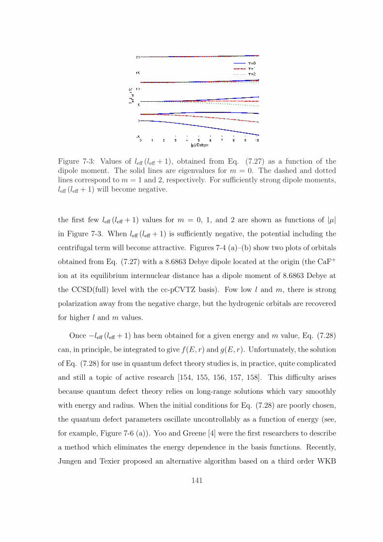
Figure 7-3: Values of leff (leff + 1), obtained from Eq. (7.27) as a function of thedipole moment. The solid lines are eigenvalues for m = 0. The dashed and dottedlines correspond to m = 1 and 2, respectively. For sufficiently strong dipole moments,leff (leff + 1) will become negative.
the first few leff (leff + 1) values for m = 0, 1, and 2 are shown as functions of |µ|in Figure 7-3. When leff (leff + 1) is sufficiently negative, the potential including the
centrifugal term will become attractive. Figures 7-4 (a)–(b) show two plots of orbitals
obtained from Eq. (7.27) with a 8.6863 Debye dipole located at the origin (the CaF+
ion at its equilibrium internuclear distance has a dipole moment of 8.6863 Debye at
the CCSD(full) level with the cc-pCVTZ basis). Fow low l and m, there is strong
polarization away from the negative charge, but the hydrogenic orbitals are recovered
for higher l and m values.
Once −leff (leff + 1) has been obtained for a given energy and m value, Eq. (7.28)
can, in principle, be integrated to give f(E, r) and g(E, r). Unfortunately, the solution
of Eq. (7.28) for use in quantum defect theory studies is, in practice, quite complicated
and still a topic of active research [154, 155, 156, 157, 158]. This difficulty arises
because quantum defect theory relies on long-range solutions which vary smoothly
with energy and radius. When the initial conditions for Eq. (7.28) are poorly chosen,
the quantum defect parameters oscillate uncontrollably as a function of energy (see,
for example, Figure 7-6 (a)). Yoo and Greene [4] were the first researchers to describe
a method which eliminates the energy dependence in the basis functions. Recently,
Jungen and Texier proposed an alternative algorithm based on a third order WKB
141
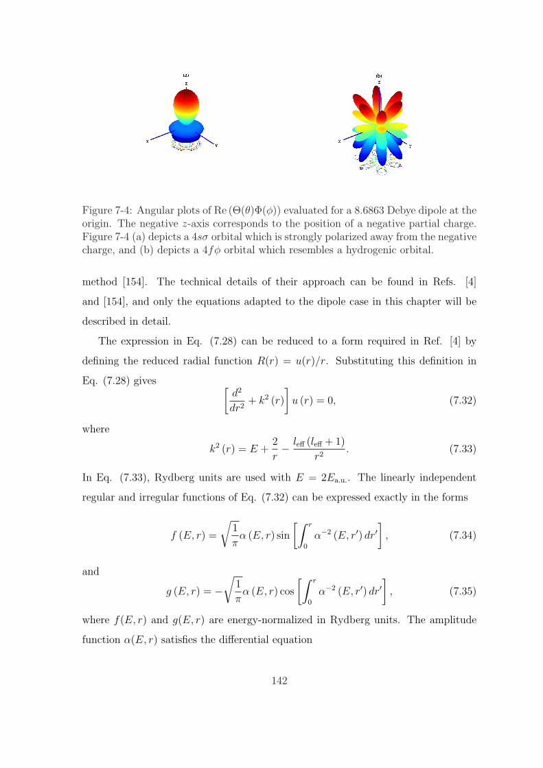
Figure 7-4: Angular plots of Re (Θ(θ)Φ(φ)) evaluated for a 8.6863 Debye dipole at theorigin. The negative z-axis corresponds to the position of a negative partial charge.Figure 7-4 (a) depicts a 4sσ orbital which is strongly polarized away from the negativecharge, and (b) depicts a 4fφ orbital which resembles a hydrogenic orbital.
method [154]. The technical details of their approach can be found in Refs. [4]
and [154], and only the equations adapted to the dipole case in this chapter will be
described in detail.
The expression in Eq. (7.28) can be reduced to a form required in Ref. [4] by
defining the reduced radial function R(r) = u(r)/r. Substituting this definition in
Eq. (7.28) gives [d2
dr2+ k2 (r)
]u (r) = 0, (7.32)
where
k2 (r) = E +2
r− leff (leff + 1)
r2. (7.33)
In Eq. (7.33), Rydberg units are used with E = 2Ea.u.. The linearly independent
regular and irregular functions of Eq. (7.32) can be expressed exactly in the forms
f (E, r) =
√1
πα (E, r) sin
[∫ r
0
α−2 (E, r′) dr′]
, (7.34)
and
g (E, r) = −√
1
πα (E, r) cos
[∫ r
0
α−2 (E, r′) dr′]
, (7.35)
where f(E, r) and g(E, r) are energy-normalized in Rydberg units. The amplitude
function α(E, r) satisfies the differential equation
142

d2α (r)
dr2+ k2 (r) α (r) = α−3 (r) . (7.36)
Therefore, obtaining f(E, r) and g(E, r) amounts to solving Eq. (7.36) and substitut-
ing the result into the definitions in Eqs. (7.34)–(7.35). It is important to note that
the solution of Eq.(7.36) in itself does not guarantee that the energy dependences will
be minimized. Their purpose in Ref. [4] is to provide the boundary conditions α (rc)
and α′ (rc) at a radius rc, which minimizes the oscillations as a function of energy.
The solution proposed by Yoo and Greene is to choose rc at the potential minimum
or at a small radius if the potential has no minimum. After a lengthy derivation,
the numerical values of α (rc) and α′ (rc) can be obtained by integrating Eq. (7.36)
inward from a large radius, rf , (around 1000 Bohrs) using the boundary conditions:
α (rf ) = k−1/2 (rf ) , E > 0, (7.37)
α′ (rf ) =d
dr
[k−1/2 (r)
]rf
, E > 0. (7.38)
This procedure is carried out at several values of E > 0, and the data points are
fitted and extrapolated to negative energies below threshold. Figure 7-5 illustrates
this procedure for a Coulomb potential with l = 1. The values of α(rc) are determined
at positive energies using Eqs. (7.37)–(7.38), and are fitted to a spline which smoothly
extrapolates to negative energies. A similar procedure is used for α′(rc).
Once this procedure is finished, one has all the necessary boundary conditions to
integrate Eq. (7.36) smoothly for arbitrary energy. The accuracy of this procedure is
best illustrated by plotting the “accumulated phase” β(E)/π defined by
β (E) /π =1
π
∫ ∞
0
α−2 (E, r) dr. (7.39)
The oscillations of β(E) qualitatively measure the energy-dependence of the basis
functions f(E, r) and g(E, r) (see Eqs. (7.34)–(7.35)). When the basis functions
f(E, r) and g(E, r) are strongly energy-dependent, this translates into large oscil-
lations in β(E), which one would like to diminish as much as possible. Figures
143

Figure 7-5: Optimal values of α(rc) as a function of energy for a l = 1 Coulombpotential. The circles at E > 0 were determined by integrating Eq. (7.36) using theboundary conditions in Eqs. (7.37)–(7.38). The solid curve is a spline fit to the circlesonly which smoothly extrapolates to E < 0.
7-6 (a)–(b) show plots of β(E) as a function of energy for a pure l = 2 Coulomb
potential. The accumulated phase β(E)/π is analytically known for the Coulomb
potential and is given by βCoulomb(E)/π = ν − l = (−E)−1/2 − l in Rydberg units
[4]. Therefore, by plotting the deviation from the analytically known accumulated
phase, β(E)/π − (ν − l), one can compare the quality of various numerical methods.
Figure 7-6 (a) shows deviations, β(E)/π − (ν − l), calculated from the extrapolation
procedure described previously (full curves) and using a zero-order WKB approxima-
tion for α(rc) and α′(rc) described in Ref. [4] (broken curves). At the energies ν = n
with n an integer, the deviation for both methods is exactly zero, as they must be
since these are true bound state eigenvalues of the Coulomb potential (E = −1/n2).
However, it is apparent in Figure 7-6 (a) that the deviations are very small for the ex-
trapolation procedure in comparison to the larger oscillations obtained with a WKB
method. In fact, the oscillations from the extrapolation procedure are unnoticeable
in Figure 7-6 (a), and one must magnify the vertical scale by an order of magnitude
to observe them in Figure 7-6 (b). Therefore, by enforcing these optimal boundary
conditions in Eq. (7.36), the functions f(E, r) and g(E, r) can be obtained as smooth
and weakly-dependent functions of the energy. For these reasons, the extrapolation
procedure described here (along with the solution to Eq. (7.27)) is currently be-
144

Figure 7-6: (a) Deviations between a numerically calculated l = 2 Coulomb phaseβ(E)/π and its analytical value ν − l. The dashed curve was obtained using a WKBboundary condition to approximate α(rc) at the minimum of the effective potential[4]. The solid curve was obtained from the extrapolated boundary condition describedin this chapter. (b) Magnified plot of Figure 7-6 (a).
ing used to obtain an optimal set of continuum functions incorporating the dipole
interaction.
7.5 The Finite Element Approach
Now that the PDE’s are specified (Section 7.3) and their boundary conditions known
(Section 7.4), one can finally discuss their numerical solution. The coupled, two-
dimensional system of PDE’s in Eqs. (7.22)–(7.23) subject to the complicated bound-
ary conditions of Section 7.4 are most easily solved using finite element methods. The
central idea of the finite element method is the use of simple basis sets which are lo-
calized only within small regions. Therefore, by using many “elements” over which
the basis functions are defined, it is possible to reproduce very complex features of the
differential equation solution. This basic idea is most easily understood in the follow-
ing one-dimensional example. The simplest basis sets in one dimension are piecewise
linear functions Fk whose value is 1 at xk and 0 at every xj where j 6= k; i.e.,
Fk(x) =
x−xk−1
xk−xk−1, if x ∈ [xk−1, xk],
xk+1−x
xk+1−xk, if x ∈ [xk, xk+1],
0, otherwise.
(7.40)
145
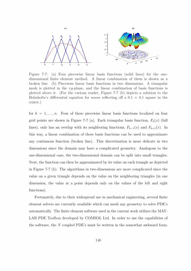
Figure 7-7: (a) Four piecewise linear basis functions (solid lines) for the one-dimensional finite element method. A linear combination of them is shown as abroken line. (b) Piecewise linear basis functions in two dimensions. A triangularmesh is plotted in the xy-plane, and the linear combination of basis functions isplotted above it. (For the curious reader, Figure 7-7 (b) depicts a solution to theHelmholtz’s differential equation for waves reflecting off a 0.1 × 0.1 square in thecenter.)
for k = 1, . . . , n. Four of these piecewise linear basis functions localized on four
grid points are shown in Figure 7-7 (a). Each triangular basis function, Fk(x) (full
lines), only has an overlap with its neighboring functions, Fk−1(x) and Fk+1(x). In
this way, a linear combination of these basis functions can be used to approximate
any continuous function (broken line). This discretization is more delicate in two
dimensions since the domain may have a complicated geometry. Analogous to the
one-dimensional case, the two-dimensional domain can be split into small triangles.
Next, the function can then be approximated by its value on each triangle as depicted
in Figure 7-7 (b). The algorithms in two-dimensions are more complicated since the
value on a given triangle depends on the value on the neighboring triangles (in one
dimension, the value at a point depends only on the values of the left and right
functions).
Fortunately, due to their widespread use in mechanical engineering, several finite
element solvers are currently available which can mesh any geometry to solve PDE’s
automatically. The finite element software used in the current work utilizes the MAT-
LAB PDE Toolbox developed by COMSOL Ltd. In order to use the capabilities of
the software, the N coupled PDE’s must be written in the somewhat awkward form:
146

−∇ · (c⊗∇u) + au = f , (7.41)
where c is an N -by-N -by-2-by-2 tensor. In the notation of the MATLAB PDE Tool-
box, the expression ∇ · (c⊗∇u) refers to the N × 1 matrix with (i, 1)-component
N∑j=1
(∂
∂xci,j,1,1
∂
∂x+
∂
∂xci,j,1,2
∂
∂y+
∂
∂yci,j,2,1
∂
∂x+
∂
∂yci,j,2,2
∂
∂y
)uj. (7.42)
The variable, a, denotes an N × N matrix, and both u and f are column vectors
of length N . For the special case of the electron scattering PDE’s specified in Eqs.
(7.22)–(7.23), the c tensor is diagonal with elements
ci,j,k,l = −δi,j
11−η2 0
0 1r2
, (7.43)
and a is given by the symmetric (Nocc + 1)× (Nocc + 1) matrix
a =
1−m2
r2(1−η2)2+ k2−2V (v)
1−η2
2u1(v)
r(1−η2)3/2
2u2(v)
r(1−η2)3/2 · · · 2uNocc (v)
r(1−η2)3/2
2u1(v)
r(1−η2)3/2
1−(m−m1)2
r2(1−η2)20 · · · 0
2u2(v)
r(1−η2)3/2 0 1−(m−m2)2
r2(1−η2)2· · · 0
......
.... . .
...
2uNocc (v)
r(1−η2)3/2 0 0 · · · 1−(m−mNocc)2
r2(1−η2)2
. (7.44)
In addition, u is the (Nocc + 1) column vector given by
u =
f (m) (v)
w(m)1 (v)
w(m)2 (v)
...
w(m)Nocc
(v)
, (7.45)
and f is a (Nocc + 1) column vector of zeros.
147
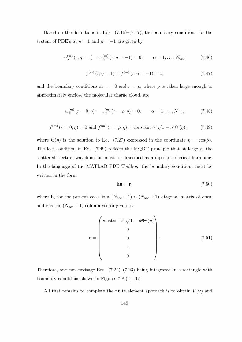
Based on the definitions in Eqs. (7.16)–(7.17), the boundary conditions for the
system of PDE’s at η = 1 and η = −1 are given by
w(m)α (r, η = 1) = w(m)
α (r, η = −1) = 0, α = 1, . . . , Nocc, (7.46)
f (m) (r, η = 1) = f (m) (r, η = −1) = 0, (7.47)
and the boundary conditions at r = 0 and r = ρ, where ρ is taken large enough to
approximately enclose the molecular charge cloud, are
w(m)α (r = 0, η) = w(m)
α (r = ρ, η) = 0, α = 1, . . . , Nocc, (7.48)
f (m) (r = 0, η) = 0 and f (m) (r = ρ, η) = constant×√
1− η2Θ (η) , (7.49)
where Θ(η) is the solution to Eq. (7.27) expressed in the coordinate η = cos(θ).
The last condition in Eq. (7.49) reflects the MQDT principle that at large r, the
scattered electron wavefunction must be described as a dipolar spherical harmonic.
In the language of the MATLAB PDE Toolbox, the boundary conditions must be
written in the form
hu = r, (7.50)
where h, for the present case, is a (Nocc + 1) × (Nocc + 1) diagonal matrix of ones,
and r is the (Nocc + 1) column vector given by
r =
constant×√
1− η2Θ (η)
0
0...
0
. (7.51)
Therefore, one can envisage Eqs. (7.22)–(7.23) being integrated in a rectangle with
boundary conditions shown in Figures 7-8 (a)–(b).
All that remains to complete the finite element approach is to obtain V (v) and
148

Figure 7-8: (a) Boundary conditions for integrating Eqs. (7.22)–(7.23) using a sparsefinite element mesh. (b) A more refined version of the triangular mesh shown inFigure 7-8 (a).
u(v). It is important to note that the entire derivation in Section 7.3 relies on
expressing both V (v) and u(v) in terms of cylindrically symmetric functions with the
form f(r, η)eimφ. Unfortunately, none of the widely used quantum chemistry codes
use complex-valued basis functions to express the bound orbitals u(v). Instead, these
programs perform calculations with Cartesian Gaussians of the form
xlAym
A znAe−αr2
A , (7.52)
where xA, yA, and zA are the components of a position vector rA relative to A
(rA = r − A), and l, m, and n are integers. Without going into further details here,
one must transform the Cartesian orbitals u(v) to pure cylindrical functions using
the properties of the spherical harmonics. The procedure for obtaining V (v) is to
convert both terms in Eq. (7.9) to pure cylindrical functions. The second term in
Eq. (7.9) is easily converted:
2∑i=1
Zi
|r−Ri| =2∑
i=1
Zi√r2 − 2zirη + z2
j
. (7.53)
The integral term in Eq. (7.9) can be calculated analytically using Cartesian Gaus-
sians [126], and the final result, which is a function of the scattered electron coordinate
r, can be converted to pure cylindrical functions as in Eq. (7.53).
149

7.6 Extracting the K matrix
Since the Θl(θ) solutions of Eq. (7.27) form a complete set, the finite element solu-
tions, f(m)l (v), can be expanded as
f(m)l (v)
r√
1− η2=
f(m)l (r, θ)
r sin θ=
∑
l′f
(m)l′ (r) Θl′ (θ), (7.54)
where f(m)l (v) denotes a particular solution from the finite element method with the
boundary condition f(m)l (r = ρ, η) = constant×
√1− η2Θl (η). In Eq. (7.54), f
(m)l′ (r)
is only a function of r. Multiplying both sides of Eq. (7.54) by Θl(θ) sin θ gives
f(m)l (r, θ) Θl (θ)
r=
∑
l′f
(m)l′ (r) Θl′ (θ) Θl (θ) sin θ. (7.55)
Since the solutions to Eq. (7.27), Θl(θ), are also orthogonal with the weighting
function sin θ, both sides of Eq. (7.55) can be integrated to give
f(m)l (r) =
∫ π
0
f(m)l (r, θ) Θl (θ)
rdθ. (7.56)
The MQDT method gives an additional equation for f(m)l (r, θ):
f(m)l (v)
r√
1− η2=
f(m)l (r, θ)
r sin θ
=∑
l′
[Al,l′
fl′ (E, r)
r+ Bl,l′
gl′ (E, r)
r
]Θl′ (θ), r À R,
(7.57)
where the scattering reaction matrix K, is given by
K = A−1B. (7.58)
Comparing Eqs. (7.54) and (7.57) gives
f(m)l′ (r) = Al,l′
fl′ (E, r)
r+ Bl,l′
gl′ (E, r)
r, r À R. (7.59)
150

Substituting the result of Eq. (7.56) in Eq. (7.59) gives
∫ π
0
f(m)l (r, θ) Θl (θ)dθ = Al,l′fl′ (E, r) + Bl,l′gl′ (E, r) , r À R. (7.60)
The continuum functions fl(E, r) and gl(E, r) can be calculated using the methods
described in Section 7.4. The integral on the left hand side of Eq. (7.60) can also
be computed once the solution f(m)l (r, θ) is obtained from the finite element method.
Therefore, to determine the matrix elements Al,l′ and Bl,l′ (and hence K), one can
choose two large values of r, such as r = ρ and r = ρ−∆r, and evaluate Eq. (7.60).
For a given value of l, this procedure results in two equations with two unknowns
which can be solved simultaneously to obtain Al,l′ and Bl,l′ . The remaining matrix
elements Al,l′ and Bl,l′ can be obtained by re-solving the finite element equations for
different values of l and performing the previously described procedure. This finally
completes the method for determining the K matrix from a multi-electron approach.
7.7 Conclusion
This chapter has thoroughly described a procedure to obtain the reaction matrix
K for electron scattering in highly polar diatomics. The technique makes use of
transforming an integro-differential equation to a system of two-dimensional PDE’s
which have no integral terms. A numerical method to reduce the energy-dependent
oscillations and dipole interactions of the continuum functions is also presented for use
in the current study. The resulting equations and boundary conditions are particularly
suited for widely available finite element solvers. Finally, the methods outlined in this
chapter are currently in the finishing stages of completion and further applications
are forthcoming.
151

152

Chapter 8
Conclusion
8.1 Summary
The physical properties of three very different chemical systems have been considered
in this thesis: (1) large-amplitude vibrations on ground-state singlet surfaces, (2) the
photophysics of electronically excited triplet states germane to doorway-mediated
intersystem crossing, and (3) electron-molecule collisions of Rydberg states. On a
practical level, each of these separate chemical systems requires a completely differ-
ent computational approach to describe their complicated nature. On a conceptual
level, however, these studies share a common philosophical framework: all of these
examples are closely connected to experimental observables or have some connection
to chemically intuitive models. For example, Chapters 2–4 illustrate the intuitive
idea that when a large-amplitude motion alters a molecular geometry, the electronic
structure of the molecule changes as well. This change in electronic structure conveys
barrier-relevant information to the spectroscopist. Chapter 5 demonstrates the use of
a simple two-dimensional model to decouple two electronically excited triplet states.
This simple but powerful model suggests a plausible vibrational assignment in the
dense forest of other nearly degenerate vibrational states. Chapters 6–7, which seem
to address the most complicated of all the systems presented here, are actually based
on the simplest idea: Rydberg states can be described as hydrogenic orbitals because
scattering is a localized process. The strong electron-nuclear interactions occur during
153

a short period of time and are confined to a limited region of space. It is these local-
ized interactions which alter a Rydberg electron’s global trajectory in free space and
provide a mechanism for energy exchange between the Rydberg electron and the ion
core. The simple intuitive models coupled with the rigorous theoretical approaches
presented in these studies make them useful tools for further developments in both
theory and experiment.
8.2 Future Directions
Although this thesis has utilized the rigorous tools of quantum chemistry to describe
various spectroscopic properties, it would be deceptive to state that these studies
are now complete. For instance, the one-dimensional dipole moments presented in
Chapter 3 provide insight into the local-bending dipoles but do not capture any
dependencies on other anharmonic or Coriolis couplings. For this reason, the one-
dimensional dipole moments of vibrationally excited acetylene are currently being
compared with full-dimensional ab initio calculations from Prof. Hua Guo at the
University of New Mexico (Figure 8-1). Similar to the one-dimensional calculation,
the preliminary full-dimensional calculations show exceptionally large dipole moments
for the lowest members of a pure-bending polyad.
On a more practical note, the vibrationally excited levels of S0 acetylene must be
experimentally accessed through stimulated emission pumping (SEP) from selected
vibrational levels of the trans-bent S1 excited state of acetylene (cf. Figure 5-1). Con-
sequently, a comprehensive understanding of the anharmonic and Coriolis couplings
on the S1 surface is necessary to experimentally locate special eigenstates that can
serve as “local-bender plucks” for S0 local-bender states. The characterization of the
acetylene S1 surface is an ongoing collaboration with Prof. John F. Stanton at the
University of Texas at Austin.
Finally, the techniques outlined in Chapter 7 are in their final stages of develop-
ment and would be the first ab initio (as opposed to an effective potential) MQDT
study on the CaF molecule. A less ambitious approach to this problem is to refine
154
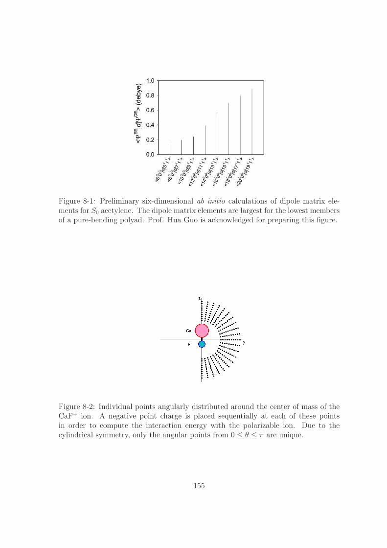
Figure 8-1: Preliminary six-dimensional ab initio calculations of dipole matrix ele-ments for S0 acetylene. The dipole matrix elements are largest for the lowest membersof a pure-bending polyad. Prof. Hua Guo is acknowledged for preparing this figure.
Figure 8-2: Individual points angularly distributed around the center of mass of theCaF+ ion. A negative point charge is placed sequentially at each of these pointsin order to compute the interaction energy with the polarizable ion. Due to thecylindrical symmetry, only the angular points from 0 ≤ θ ≤ π are unique.
155

the parameters in the effective potential using ab initio calculations and re-calculate
the MQDT equations with this new effective potential. The strategy is to adjust the
parameters to fit ab initio energies of point charges angularly distributed around the
CaF+ ion (Figure 8-2). Once this fit is finished, these parameters can be modified and
compared with experimental data. This approach of refining the effective potential
is an ongoing collaboration with Dr. Stephen L. Coy.
156

Appendix A
Expansion of the Internal
Coordinate Hamiltonian
This appendix contains a detailed derivation of Eq. (2.8) in Chapter 2.
The quantum mechanical kinetic energy operator for the motion of the nuclei is
given by
T = 12
4∑
d,e=1
µ1/4(Πd − πd
)µdeµ
−1/2(Πe − πe
)µ1/4+ 1
2
3N−7∑
k=1
µ1/4Pkµ−1/2Pkµ
1/4. (A.1)
This expression can be expanded into the following form:
T = 12µ1/4
3∑
d,e=1
(Πd − πd
)µdeµ
−1/2(Πe − πe
)µ1/4
+ 12µ1/4
3∑
d=1
(Πd − πd
)µdsµ
−1/2 (ps − πs) µ1/4
+ 12µ1/4
3∑
d=1
(ps − πs) µsdµ−1/2
(Πd − πd
)µ1/4
+ 12µ1/4 (ps − πs) µssµ
−1/2 (ps − πs) µ1/4 + 12µ1/4
3N−7∑
k=1
Pkµ−1/2Pkµ
1/4,
(A.2)
where the variable “s” has been used in place of the subscript “4” for notational
convenience in the previous expression. If µde and µ are expanded in the vibrational
157

normal coordinates and only the first term depending on s is retained (cf. Eq. (2.7)),
then µde and µ are solely functions of s, and the following commutation properties
hold:
[Πa, µde
]=
[Πa, µ
]= 0, (a = 1, 2, 3) and (d, e = 1, 2, 3, 4) , (A.3)
[πa, µde] = [πa, µ] = 0, (a = 1, 2, 3, 4) and (d, e = 1, 2, 3, 4) , (A.4)
[Pk, µ
]= 0, (A.5)
[µde, µ] = 0, (d, e = 1, 2, 3, 4) . (A.6)
Using these commutation rules in Eq. (A.2) gives
T = 12
3∑
d,e=1
µde
(Πd − πd
)(Πe − πe
)
+ 12µ−1/4
3∑
d=1
µds
(Πd − πd
)(ps − πs) µ1/4
+ 12µ1/4
3∑
d=1
(ps − πs) µsdµ−1/4
(Πd − πd
)
+ 12µ1/4 (ps − πs) µssµ
−1/2 (ps − πs) µ1/4 + 12
3N−7∑
k=1
P 2k .
(A.7)
The notation of Eq. (A.7) can be condensed further by defining the operators
Ja = Πa − πa, (a = 1, 2, 3) , (A.8)
Js = ps − πs, (A.9)
which obey the commutation rules
[Ja, Js
]= 0, (a = 1, 2, 3) , (A.10)
[Ja, µde
]=
[Ja, µ
]= 0, (a = 1, 2, 3) and (d, e = 1, 2, 3, 4) . (A.11)
158
Using definitions (A.8)–(A.9), Eq. (A.7) can be rearranged in the following form
T = 12
3∑
d,e=1
µdeJdJe + 12µ−1/4
3∑
d=1
µdsJdJsµ1/4 + 1
2µ1/4
3∑
d=1
Jsµsdµ−1/4Jd
+ 12µ1/4Jsµssµ
−1/2Jsµ1/4 + 1
2
3N−7∑
k=1
P 2k .
(A.12)
Since Js does not commute with µde or µ, Eq. (A.12) can be written in terms of
commutators between Js, µde, and µ,
T = 12
3∑
d,e=1
µdeJdJe + 12µ−1/4
3∑
d=1
µdsJd
([Js, µ
1/4]
+ µ1/4Js
)
+ 12µ1/4
3∑
d=1
([Js, µsdµ
−1/4]
+ µsdµ−1/4Js
)Jd
+ 12µ1/4Jsµssµ
−1/2Jsµ1/4 + 1
2
3N−7∑
k=1
P 2k .
(A.13)
Using commutator Eqs. (A.10)–(A.11) in Eq. (A.13) gives
T = 12
3∑
d,e=1
µdeJdJe + 12µ−1/4
3∑
d=1
µds
[Js, µ
1/4]Jd + 1
2
3∑
d=1
µdsJdJs
+ 12µ1/4
3∑
d=1
[Js, µsdµ
−1/4]Jd + 1
2
3∑
d=1
µsdJsJd
+ 12µ1/4Jsµssµ
−1/2Jsµ1/4 + 1
2
3N−7∑
k=1
P 2k .
(A.14)
The second commutator in Eq. (A.14) can be simplified using the commutation
identity [A, BC
]=
[A, B
]C + B
[A, C
]. (A.15)
159

Therefore,
T = 12
3∑
d,e=1
µdeJdJe + 12
3∑
d=1
µdsJdJs + 12
3∑
d=1
µsdJsJd
+ 12µ−1/4
3∑
d=1
µds
[Js, µ
1/4]Jd + 1
2µ1/4
3∑
d=1
[Js, µsd
]µ−1/4Jd
+ 12µ1/4
3∑
d=1
µsd
[Js, µ
−1/4]Jd + 1
2µ1/4Jsµssµ
−1/2Jsµ1/4 + 1
2
3N−7∑
k=1
P 2k .
(A.16)
The second to last term in Eq. (A.16) can be expanded in the following form:
12µ1/4Jsµssµ
−1/2Jsµ1/4
= 12µ1/4Jsµssµ
−1/2([
Js, µ1/4
]+ µ1/4Js
)
= 12µ1/4Jsµssµ
−1/2[Js, µ
1/4]
+ 12µ1/4Jsµssµ
−1/4Js
= 12µ1/4
([Js, µssµ
−1/2[Js, µ
1/4]]
+ µssµ−1/2
[Js, µ
1/4]Js
)
+ 12µ1/4
([Js, µssµ
−1/4]
+ µssµ−1/4Js
)Js
= 12µ1/4
[Js, µssµ
−1/2[Js, µ
1/4]]
+ 12µssµ
−1/4[Js, µ
1/4]Js
+ 12µ1/4
[Js, µssµ
−1/4]Js + 1
2µssJsJs
= 12µ1/4
[Js, µssµ
−1/2[Js, µ
1/4]]
+ 12µssµ
−1/4[Js, µ
1/4]Js
+ 12µ1/4
[Js, µss
]µ−1/4Js + 1
2µ1/4µss
[Js, µ
−1/4]Js + 1
2µssJsJs.
(A.17)
Substituting Eq. (A.17) in Eq. (A.16) and collecting terms gives
T = 12
4∑
d,e=1
µdeJdJe + 12µ−1/4
4∑
d=1
µds
[Js, µ
1/4]Jd
+ 12µ1/4
4∑
d=1
[Js, µsd
]µ−1/4Jd + 1
2µ1/4
4∑
d=1
µsd
[Js, µ
−1/4]Jd
+ 12µ1/4
[Js, µssµ
−1/2[Js, µ
1/4]]
+ 12
3N−7∑
k=1
P 2k .
(A.18)
The second term in Eq. (A.18) can be rearranged using the commutation identity in
160
Eq. (A.15)
12µ−1/4
4∑
d=1
µds
[Js, µ
1/4]Jd
= 12
4∑
d=1
µdsµ−1/4
[Js, µ
1/4]Jd
= 12
4∑
d=1
µds
[Js, 1
]Jd − 1
2
4∑
d=1
µds
[Js, µ
−1/4]µ1/4Jd
= −12
4∑
d=1
µds
[Js, µ
−1/4]µ1/4Jd.
(A.19)
Substituting Eq. (A.19) in Eq. (A.18) gives
T = 12
4∑
d,e=1
µdeJdJe − 12
4∑
d=1
µds
[Js, µ
−1/4]µ1/4Jd
+ 12µ1/4
4∑
d=1
[Js, µsd
]µ−1/4Jd + 1
2µ1/4
4∑
d=1
µsd
[Js, µ
−1/4]Jd
+ 12µ1/4
[Js, µssµ
−1/2[Js, µ
1/4]]
+ 12
3N−7∑
k=1
P 2k .
(A.20)
The commutators in Eq. (A.20) can be significantly simplified using Eq. (A.9) and
commutator Eq. (A.4). For example,
[Js, µ
]= [ps − πs, µ]
= [ps, µ]− [πs, µ]
= [ps, µ] .
(A.21)
Commutators involving µsd and other functions of µ are similar. Re-expressing Eq.
(A.20) in terms of the original operators defined in Eqs. (A.8)–(A.9) gives
161
T = 12
4∑
d,e=1
µde
(Πd − πd
)(Πe − πe
)− 1
2
4∑
d=1
µds
[ps, µ
−1/4]µ1/4
(Πd − πd
)
+ 12µ1/4
4∑
d=1
[ps, µsd] µ−1/4
(Πd − πd
)
+ 12µ1/4
4∑
d=1
µsd
[ps, µ
−1/4] (
Πd − πd
)+ 1
2µ1/4
[ps, µssµ
−1/2[ps, µ
1/4]]
+ 12
3N−7∑
k=1
P 2k .
(A.22)
To simplify Eq. (A.22) even further one must remember that ps = −i~∂/∂s is a
differential operator, and commutators such as[ps, µ
−1/4]
can be written as
[ps, µ
−1/4]
= psµ−1/4 − µ−1/4ps
=(psµ
−1/4)
+ µ−1/4ps − µ−1/4ps
=(psµ
−1/4),
(A.23)
where the product rule was used in the second step since ps is an operator which
operates on some function to the right; that is, the operator ps operates only within
the parentheses. Therefore, remembering the previous convention, one can replace all
the commutators in Eq. (A.22) with parentheses:
T = 12
4∑
d,e=1
µde
(Πd − πd
)(Πe − πe
)− 1
2
4∑
d=1
µds
(ps, µ
−1/4)µ1/4
(Πd − πd
)
+ 12µ1/4
4∑
d=1
(ps, µsd) µ−1/4(Πd − πd
)
+ 12µ1/4
4∑
d=1
µsd
(ps, µ
−1/4) (
Πd − πd
)+ 1
2µ1/4
(ps, µssµ
−1/2(ps, µ
1/4))
+ 12
3N−7∑
k=1
P 2k .
(A.24)
Since the tensor µde is symmetric, µds = µsd. Furthermore, since the quantities within
162

parentheses in Eq. (A.24) are solely functions of s, they commute with µ, and the
second and fourth terms of Eq. (A.24) cancel. Simplifying Eq. (A.24) finally yields
T = 12
4∑
d,e=1
µde
(Πd − πd
)(Πe − πe
)+ 1
2
4∑
d=1
(psµsd)(Πd − πd
)
+ 12µ1/4
(psµssµ
−1/2(psµ
1/4))
+ 12
3N−7∑
k=1
P 2k ,
(A.25)
which is Eq. (2.8) in Chapter 2 as promised.
163

164
Appendix B
Computer Codes for Calculating
Vibrational Overlap Integrals
This appendix contains source codes for calculating the vibrational overlap integrals
described in Chapter 5. The MATLAB m-file overlap integral.m can calculate vi-
brational overlap integrals for any general molecule given L′, L, R′eq, Req, m, and
n as inputs. The m-file make overlap table.m demonstrates how to use over-
lap integral.m by generating Table 5.6 as a sample output. The m-files
b matrix acetylene.m and load acetylene data.m are specific to acetylene and
are required by make overlap table.m to run correctly. All files in this appendix
are available via the Internet [112] and were successfully tested on MATLAB Version
7.3 with the Symbolic Math Toolbox.
B.1 overlap integral.m
1 function overlap=overlap_integral(L_prime,L,R_eq_prime,R_eq,...
omega_prime,omega,m,n)
%
% This function (overlap_integral.m) calculates the vibrational
% overlap integral between two nuclear wavefunctions using the
% formalism developed by Sharp and Rosenstock (J. Chem. Phys.,
% 41:3453, 1964). This function requires the MATLAB Symbolic
165
% Toolbox in order to run correctly and needs the following data
% as inputs:
10 %
% L_prime: (3N-6)x(3N-6) L matrix of the initial vibrational
% state. The L matrix relates the normal mode coordinates to the
% internal displacement coordinates and is defined in Eq. (9) of
% Sharp and Rosenstock.
%
% L: (3N-6)x(3N-6) L matrix of the final vibrational state. See
% description for L_prime.
%
% R_eq_prime: (3N-6)x1 column vector whose components are the
20 % equilibrium internal coordinates of the initial state. The
% ordering of the (3N-6) components must correspond with the
% (3N-6) rows of L_prime.
%
% R_eq: (3N-6)x1 column vector whose components are the
% equilibrium internal coordinates of the final state. The
% ordering of the (3N-6) components must correspond with the
% (3N-6) rows of L.
%
% omega_prime: 1x(3N-6) row vector whose components are the
30 % normal mode frequencies of the initial state. The frequencies
% must be in units of (omega_prime/hbar): amu^(-1)*Angstrom^(-2).
% The ordering of the (3N-6) components must correspond with the
% (3N-6) columns of L_prime.
%
% omega: 1x(3N-6) row vector whose components are the normal mode
% frequencies of the final state. The frequencies must be in
% units of (omega/hbar): amu^(-1)*Angstrom^(-2). The ordering of
% the (3N-6) components must correspond with the (3N-6) columns
% of L.
40 %
% m: 1x(3N-6) row vector whose components are the vibrational
% quanta in each of the (3N-6) oscillators of the initial state.
% The ordering of the (3N-6) components must correspond with the
% (3N-6) columns of omega_prime.
%
% n: 1x(3N-6) row vector whose components are the vibrational
% quanta in each of the (3N-6) oscillators of the final state.
% The ordering of the (3N-6) components must correspond with the
% (3N-6) columns of omega.
50R=R_eq-R_eq_prime; % Eq. (8) of Sharp and Rosenstock
166

J=inv(L_prime)*L; % Eq. (11) of Sharp and Rosenstock
K=inv(L_prime)*R; % Eq. (11) of Sharp and Rosenstock
gamma_prime=diag(omega_prime);
% (3N-6)x(3N-6) diagonal matrix of initial frequencies
gamma=diag(omega);
% (3N-6)x(3N-6) diagonal matrix of final frequencies
60Z=J’*gamma_prime*J+gamma;
% This quantity appears several times in Eqs. (21a) - (21e) of
% Sharp and Rosenstock. This variable is computed here once to
% save some computer time and simplify the following lines of
% code.
A=2*sqrt(gamma_prime)*J*inv(Z)*J’*sqrt(gamma_prime)...
-eye(length(omega));
% Eq. (21a) of Sharp and Rosenstock
70 B=-2*sqrt(gamma_prime)*(J*inv(Z)*J’*gamma_prime...
-eye(length(omega)))*K;
% Eq. (21b) of Sharp and Rosenstock
C=2*sqrt(gamma)*inv(Z)*sqrt(gamma)-eye(length(omega));
% Eq. (21c) of Sharp and Rosenstock
D=-2*sqrt(gamma)*inv(Z)*J’*gamma_prime*K;
% Eq. (21d) of Sharp and Rosenstock
E=4*sqrt(gamma)*inv(Z)*J’*sqrt(gamma_prime);
% Eq. (21e) of Sharp and Rosenstock
80 for i=1:length(m)
T(i,1)=sym([’t’ num2str(i)],’real’);
% initialize the T vector (Eq. (22) of Sharp and Rosenstock))
% with (3N-6) dummy symbolic variables
U(i,1)=sym([’u’ num2str(i)],’real’);
% initialize the U vector (Eq. (22) of Sharp and Rosenstock))
% with (3N-6) dummy symbolic variables
90 end
f=exp(T’*A*T+T’*B+U’*C*U+U’*D+U’*E*T);
% generating function from the right hand side of Eq. (22) of
% Sharp and Rosenstock
for i=1:length(m)
167
f=diff(f,T(i),m(i));
f=subs(f,T(i),0);
100 % take the m(i)-order derivative of the generating function
% with respect to each of the (3N-6) dummy variables in T
f=diff(f,U(i),n(i));
f=subs(f,U(i),0);
% take the n(i)-order derivative of the generating function
% with respect to each of the (3N-6) dummy variables in U
end
110 f=f/sqrt(prod(2.^(m+n).*factorial(m).*factorial(n)));
% divide the generating function with the left hand side of Eq.
% (22) of Sharp and Rosenstock
I_0=2^(length(m)/2)*det(gamma*gamma_prime)^(1/4)...
/sqrt(det(J*Z))*exp(-1/2*K’*gamma_prime*K+1/2*K’...
*gamma_prime*J*inv(Z)*J’*gamma_prime*K);
% normalization factor for the overlap integral (Eq. (21) of
% Sharp and Rosenstock). This variable is the corrected version
% of Eq. (21) in Sharp and Rosenstock which contains a misprint.
120overlap=I_0*f;
% overlap integral
168

B.2 make overlap table.m
1 function make_overlap_table
% This function (make_overlap_table.m) demonstrates how to use
% the MATLAB m-files load_acetylene_data.m, b_matrix_acetylene.m,
% and overlap_integral.m by generating Table V taken from (R. L.
% Thom, B. M. Wong, R. W. Field, and J. F. Stanton. J. Chem.
% Phys., 126:184307, 2007).
[L_internal_s1,L_internal_t3,R_eq_s1,R_eq_t3,omega_s1,...
10 omega_t3]=load_acetylene_data;
% load data for the S1 and T3 states of acetylene
m_s1=[0 0 3 0 0 0];
% 3 quanta in mode v3 for the S1 state of acetylene. Since the
% harmonic frequencies of S1 (outputted by load_acetylene_data.m)
% are in ascending numerical order, the components of m_s1
% correspond to the mode numbering scheme: [v4,v6,v3,v2,v5,v1].
n_t3_matrix=[1,2,0,1,0,0;
20 0,3,1,0,0,0;
5,0,1,0,0,0;
2,4,0,0,0,0;
1,0,0,0,1,0;
7,1,0,0,0,0;
1,0,1,1,0,0;
3,1,0,1,0,0;
0,1,2,0,0,0;
2,2,1,0,0,0;
4,3,0,0,0,0];
30 % matrix of vibrational quantum numbers for T3 which fall within
% approximately 100 cm^(-1) of 3v3 S1. Since the harmonic
% frequencies of T3 (outputted by load_acetylene_data.m) are in
% ascending numerical order, the columns of n_t3 correspond to
% the mode numbering scheme: [v6,v4,v3,v2,v5,v1].
for i=1:length(n_t3_matrix(:,1))
overlap(i)=overlap_integral(L_internal_s1,L_internal_t3,...
R_eq_s1,R_eq_t3,omega_s1,omega_t3,m_s1,n_t3_matrix(i,:));
40 % calculate the overlap integral between 3v3 S1 and each of
% the rows of n_t3_matrix
169

end
disp(’--------------------------------------------’)
disp(’ Vibrational Level Overlap with S1 3v3’)
disp(’ (v1 v2 v3 v4 v5 v6)’)
disp(’--------------------------------------------’)
50 fprintf(1, ’ %2.0f %2.0f %2.0f %2.0f %2.0f %2.0f %16.4f \n’,...
[n_t3_matrix(:,[6,4,3,2,5,1])’;overlap])
disp(’--------------------------------------------’)
% display the vibrational quantum numbers and overlaps in a table
170
B.3 load acetylene data.m
1 function [L_internal_s1,L_internal_t3,R_eq_s1,R_eq_t3,...
omega_s1,omega_t3]=load_acetylene_data
%
% This function (load_acetylene_data.m) processes and outputs the
% data needed by overlap_integral.m to calculate vibrational
% overlap integrals between the S1 and T3 states of acetylene.
% This function requires the MATLAB m-file b_matrix_acetylene.m
% in order to run correctly and outputs the following data:
%
10 % L_internal_s1: 6x6 L matrix for the S1 state of acetylene
% (atoms labeled by H3-C1-C2-H4, where H3 is bonded to C1, and H4
% is bonded to C2). The ordering of the 6 rows correspond to the
% following internal coordinates: (1) C2-C1 bond distance, (2)
% H3-C1 bond distance, (3) H4-C2 bond distance, (4) H3-C1-C2
% angle, (5) H4-C2-C1 angle, and (6) H3-C1-C2-H4 torsional angle.
%
% L_internal_t3: 6x6 L matrix for the T3 state of acetylene. The
% atom labels and the internal coordinate ordering are the same
% as the rows which comprise L_internal_s1.
20 %
% R_eq_s1: 6x1 column vector whose components are the equilibrium
% internal coordinates of the S1 state. The ordering of the 6
% components correspond to the 6 rows of L_internal_s1.
%
% R_eq_t3: 6x1 column vector whose components are the equilibrium
% internal coordinates of the T3 state. The ordering of the 6
% components correspond to the 6 rows of L_internal_t3.
%
% omega_s1: 1x6 row vector containing the harmonic frequencies of
30 % S1 (in ascending order) in units of amu^(-1)*Angtroms^(-2)
%
% omega_t3: 1x6 row vector containing the harmonic frequencies of
% T3 (in ascending order) in units of amu^(-1)*Angtroms^(-2)
hbar=1.05457266e-34;
amu=1.6605402e-27;
lightspeed=299792458e2;
angstrom=0.529177249;
40 conversion=lightspeed/hbar*amu*1e-20;
171
m_C=12; % mass of carbon in amus
m_H=1.007825035; % mass of hydrogen in amus
zmat_s1=angstrom*[1.2563457714 0.2243278705 0.0000000000
-1.2563457714 -0.2243278705 0.0000000000
2.6953689580 -1.2450027117 0.0000000000
-2.6953689580 1.2450027117 0.0000000000];
% Cartesian coordinates of the S1 state in Angstroms. The rows in
50 % zmat_s1 correspond to the atoms C1, C2, H3, and H4 where H3 is
% bonded to C1, and H4 is bonded to C2.
zmat_t3=angstrom*[1.2639239709 0.1462769266 -0.0654251864
-1.2639239709 -0.1462769266 -0.0654251864
2.8768155828 -0.7652103906 0.7790064839
-2.8768155828 0.7652103906 0.7790064839];
% Cartesian coordinates of the T3 state in Angstroms. The rows in
% zmat_t3 correspond to the atoms C1, C2, H3, and H4 where H3 is
% bonded to C1, and H4 is bonded to C2.
60N=length(zmat_s1(:,1)); % number of atoms
e12_s1=zmat_s1(2,:)-zmat_s1(1,:);
R_eq_s1(1,1)=norm(e12_s1); % C2-C1 bond length for S1
e12_s1=e12_s1/R_eq_s1(1,1); % unit vector from C1 to C2 for S1
e21_s1=-e12_s1; % unit vector from C2 to C1 for S1
e13_s1=zmat_s1(3,:)-zmat_s1(1,:);
R_eq_s1(2,1)=norm(e13_s1); % H3-C1 bond length for S1
70 e13_s1=e13_s1/R_eq_s1(2,1); % unit vector from C1 to H3 for S1
e31_s1=-e13_s1; % unit vector from H3 to C1 for S1
e24_s1=zmat_s1(4,:)-zmat_s1(2,:);
R_eq_s1(3,1)=norm(e24_s1); % H4-C2 bond length for S1
e24_s1=e24_s1/R_eq_s1(3,1); % unit vector from C2 to H4 for S1
R_eq_s1(4,1)=acos(dot(e13_s1,e12_s1));
% H3-C1-C2 angle in radians for S1
R_eq_s1(5,1)=acos(dot(e21_s1,e24_s1));
80 % H4-C2-C1 angle in radians for S1
R_eq_s1(6,1)=acos(dot(cross(e31_s1,e12_s1),...
cross(e12_s1,e24_s1))/(sin(R_eq_s1(4,1))*sin(R_eq_s1(5,1))));
% H3-C1-C2-H4 torsional angle in radians for S1
e12_t3=zmat_t3(2,:)-zmat_t3(1,:);
172

R_eq_t3(1,1)=norm(e12_t3); % C2-C1 bond length for T3
e12_t3=e12_t3/R_eq_t3(1,1); % unit vector from C1 to C2 for T3
e21_t3=-e12_t3; % unit vector from C2 to C1 for T3
90e13_t3=zmat_t3(3,:)-zmat_t3(1,:);
R_eq_t3(2,1)=norm(e13_t3); % H3-C1 bond length for T3
e13_t3=e13_t3/R_eq_t3(2,1); % unit vector from C1 to H3 for T3
e31_t3=-e13_t3; % unit vector from H3 to C1 for T3
e24_t3=zmat_t3(4,:)-zmat_t3(2,:);
R_eq_t3(3,1)=norm(e24_t3); % H4-C2 bond length for T3
e24_t3=e24_t3/R_eq_t3(3,1); % unit vector from C2 to H4 for T3
100 R_eq_t3(4,1)=acos(dot(e13_t3,e12_t3));
% H3-C1-C2 angle in radians for T3
R_eq_t3(5,1)=acos(dot(e21_t3,e24_t3));
% H4-C2-C1 angle in radians for T3
R_eq_t3(6,1)=acos(dot(cross(e31_t3,e12_t3),...
cross(e12_t3,e24_t3))/(sin(R_eq_t3(4,1))*sin(R_eq_t3(5,1))));
% H3-C1-C2-H4 torsional angle in radians for T3
omega_s1_cm=[641.5243555793 732.4065268561 1087.2531708330 ...
110 1503.9932895188 3091.3722518386 3113.8218266995];
omega_s1=conversion*omega_s1_cm;
% harmonic frequencies of S1 in amu^(-1) Angtroms^(-2)
omega_t3_cm=[397.5591668938 653.0417221433 1411.9585215773 ...
1626.8956207661 3036.4846162879 3225.8838136171];
omega_t3=conversion*omega_t3_cm;
% harmonic frequencies of T3 in amu^(-1) Angtroms^(-2)
L_cart_s1=[0.0000000000 0.0000000000 0.1968227203
120 0.0000000000 0.0000000000 0.1968227203
0.0000000000 0.0000000000 -0.6791618487
0.0000000000 0.0000000000 -0.6791618487
0.1356965875 0.1425679465 0.0000000000
0.1356965875 0.1425679465 0.0000000000
-0.4682383473 -0.4919488458 0.0000000000
-0.4682383473 -0.4919488458 0.0000000000
0.0620248472 0.3805824000 0.0000000000
-0.0620248472 -0.3805824000 0.0000000000
-0.4490122073 -0.3869082486 0.0000000000
130 0.4490122073 0.3869082486 0.0000000000
0.6756377137 0.0839708460 0.0000000000
173
-0.6756377137 -0.0839708460 0.0000000000
0.1888498906 -0.0282541255 0.0000000000
-0.1888498906 0.0282541255 0.0000000000
0.1425679465 -0.1356965875 0.0000000000
0.1425679465 -0.1356965875 0.0000000000
-0.4919488458 0.4682383473 0.0000000000
-0.4919488458 0.4682383473 0.0000000000
0.1704280896 -0.1223824165 0.0000000000
140 -0.1704280896 0.1223824165 0.0000000000
-0.4850244785 0.4698170555 0.0000000000
0.4850244785 -0.4698170555 0.0000000000];
% mass weighted Cartesian normal mode eigenvector l matrix for
% S1; this is from the standard output of ACES II which outputs
% this matrix in 3 columns corresponding to x, y, and z
L_cart_t3=[0.0869087881 0.1318727780 -0.2712668339
0.0869087881 0.1318727780 0.2712668339
-0.2998898354 -0.4550438058 0.3232212234
150 -0.2998898354 -0.4550438058 -0.3232212234
0.0845920890 0.2869702881 -0.1107145827
-0.0845920890 -0.2869702881 -0.1107145827
-0.3900441432 -0.3164640929 0.3820347598
0.3900441432 0.3164640929 0.3820347598
0.5610259535 0.1842498836 0.0714344622
-0.5610259535 -0.1842498836 0.0714344622
0.1814546585 -0.2291594167 -0.2464937041
-0.1814546585 0.2291594167 -0.2464937041
0.3684818408 -0.1988277097 -0.1241176044
160 -0.3684818408 0.1988277097 -0.1241176044
0.1164649336 0.3351008493 0.4282835920
-0.1164649336 -0.3351008493 0.4282835920
0.1739955891 -0.0658689303 0.0342824442
0.1739955891 -0.0658689303 -0.0342824442
-0.6003939268 0.2272891279 -0.2282067440
-0.6003939268 0.2272891279 0.2282067440
0.1943913023 -0.0785119452 0.0772877889
-0.1943913023 0.0785119452 0.0772877889
-0.5394169319 0.2966135359 -0.2666913529
170 0.5394169319 -0.2966135359 -0.2666913529];
% mass weighted Cartesian normal mode eigenvector l matrix for
% T3; this is from the standard output of ACES II which outputs
% this matrix in 3 columns corresponding to x, y, and z
L_cart_s1=reshape(L_cart_s1’,[3*N,3*N-6]);
% reshape the S1 l matrix to the standard 3N x (3N-6) size
174

L_cart_t3=reshape(L_cart_t3’,[3*N,3*N-6]);
% reshape the T3 l matrix to the standard 3N x (3N-6) size
180 inv_sqrt_M=diag(kron(1./sqrt([m_C,m_C,m_H,m_H]),ones(1,3)));
% diagonal 3N x 3N matrix containing the reciprocal square roots
% of the atom masses
B_s1=b_matrix_acetylene(zmat_s1); % B matrix for S1
B_t3=b_matrix_acetylene(zmat_t3); % B matrix for T3
L_internal_s1=B_s1*inv_sqrt_M*L_cart_s1; % L matrix for S1
L_internal_t3=B_t3*inv_sqrt_M*L_cart_t3; % L matrix for T3
175

B.4 b matrix acetylene.m
1 function B=b_matrix_acetylene(zmat)
%
% This function (b_matrix_acetylene.m) processes and outputs the
% B matrix for acetylene. Expressions for the B matrix elements
% were taken from Section 4-1 of (E. B. Wilson Jr., J. C. Decius,
% and P. C. Cross. Molecular Vibrations: The Theory of Infrared
% and Raman Vibrational Spectra. Dover Publications: New York,
% 1955). This function only requires the z matrix (zmat) in
% Cartesian coordinates. The rows in zmat must correspond to the
10 % atoms C1, C2, H3, and H4 where H3 is bonded to C1, and H4 is
% bonded to C2.
%
% The 6 rows of the outputted B matrix correspond to the
% following internal coordinates: (1) C2-C1 bond distance, (2)
% H3-C1 bond distance, (3) H4-C2 bond distance, (4) H3-C1-C2
% angle, (5) H4-C2-C1 angle, and (6) H3-C1-C2-H4 torsional angle.
N=length(zmat(:,1));
% initialize N to be the number of atoms
20B=zeros(3*N-6,3*N);
% initialize (3N-6)x(3N) B matrix with zeros
e12=zmat(2,:)-zmat(1,:);
e12=e12/norm(e12); % unit vector from C1 to C2
e21=-e12; % unit vector from C2 to C1
B(1,1:6)=[e21,e12];
% first row of B matrix (Eq. (3) from Wilson et. al)
30e13=zmat(3,:)-zmat(1,:);
e13=e13/norm(e13); % unit vector from C1 to H3
e31=-e13; % unit vector from H3 to C1
B(2,[1:3,7:9])=[e31,e13];
% second row of B matrix (Eq. (3) from Wilson et. al)
e24=zmat(4,:)-zmat(2,:);
e24=e24/norm(e24); % unit vector from C2 to H4
40 e42=-e24; % unit vector from H4 to C2
176

B(3,[4:6,10:12])=[e42,e24];
% third row of B matrix (Eq. (3) from Wilson et. al)
r13=norm(zmat(3,:)-zmat(1,:)); % H3-C1 bond length
r12=norm(zmat(2,:)-zmat(1,:)); % C1-C2 bond length
phi=acos(dot(e13,e12)); % H3-C1-C2 angle in radians
B(4,1:9)=[((r13-r12*cos(phi))*e13...
50 +(r12-r13*cos(phi))*e12)/(r13*r12*sin(phi)),...
(cos(phi)*e12-e13)/(r12*sin(phi)),...
(cos(phi)*e13-e12)/(r13*sin(phi))];
% fourth row of B matrix (Eqs. (5)-(7) from Wilson et. al)
r21=norm(zmat(1,:)-zmat(2,:)); % C1-C2 bond length
r24=norm(zmat(4,:)-zmat(2,:)); % H4-C2 bond length
phi=acos(dot(e21,e24)); % H4-C2-C1 angle in radians
B(5,[1:6,10:12])=[(cos(phi)*e21-e24)/(r21*sin(phi)),...
60 ((r21-r24*cos(phi))*e21...
+(r24-r21*cos(phi))*e24)/(r21*r24*sin(phi)),...
(cos(phi)*e24-e21)/(r24*sin(phi))];
% fifth row of B matrix (Eqs. (5)-(7) from Wilson et. al)
r31=r13; % C1-H3 bond length
r42=r24; % C2-H4 bond length
phi1=acos(dot(e13,e12)); % H3-C1-C2 angle in radians
phi2=acos(dot(e21,e24)); % H4-C2-C1 angle in radians
70 B(6,:)=[(r12-r31*cos(phi1))/(r12*r31*sin(phi1))...
*cross(e31,e12)/sin(phi1)+cos(phi2)/(r12*sin(phi2))...
*cross(e42,e21)/sin(phi2),...
(r21-r42*cos(phi2))/(r21*r42*sin(phi2))...
*cross(e42,e21)/sin(phi2)+cos(phi1)/(r21*sin(phi1))...
*cross(e31,e12)/sin(phi1),...
-cross(e31,e12)/(r31*(sin(phi1))^2),...
-cross(e42,e21)/(r42*(sin(phi2))^2)];
% sixth row of B matrix (Eqs. (21)-(24) from Wilson et. al)
177

178

Appendix C
Analytical Expressions for One-
and Two-Electron Integrals in K
matrix Calculations
This appendix contains closed-form analytical expressions for one- and two-electron
integrals between Cartesian Gaussians outside a finite spherical region of space. The
majority of the work in this appendix resulted from a collaboration with Dr. Serhan
N. Altunata and was published as an article in the Journal of Chemical Physics [114].
C.1 General Expansion of Cartesian Gaussian Or-
bitals
A general unnormalized Cartesian Gaussian Orbital (CGO) centered at point RP =
(XP , YP , ZP ) is given by
χP (p, q, r, a) = xpP yq
P zrP e−ar2
P , (C.1)
where xP , yP , and zP are Cartesian components relative to the point RP where
rP = (xP , yP , zP ) = (x − XP , y − YP , z − ZP ), and p, q, and r are integers greater
179
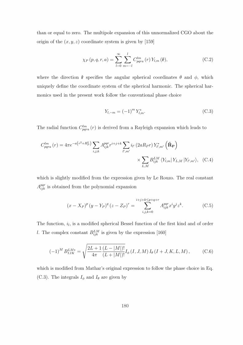
than or equal to zero. The multipole expansion of this unnormalized CGO about the
origin of the (x, y, z) coordinate system is given by [159]
χP (p, q, r, a) =∞∑
l=0
l∑
m=−l
C lmpqra (r) Yl,m (r), (C.2)
where the direction r specifies the angular spherical coordinates θ and φ, which
uniquely define the coordinate system of the spherical harmonic. The spherical har-
monics used in the present work follow the conventional phase choice
Yl,−m = (−1)m Y ∗l,m. (C.3)
The radial function C lmpqra (r) is derived from a Rayleigh expansion which leads to
C lmpqra (r) = 4πe−a(r2+R2
P )∑
i,j,k
Apqrijk ri+j+k
∑
l′,m′il′ (2aRP r) Y ∗
l′,m′
(RP
)
×∑L,M
BLMijk 〈Yl,m|YL,M |Yl′,m′〉, (C.4)
which is slightly modified from the expression given by Le Rouzo. The real constant
Apqrijk is obtained from the polynomial expansion
(x−XP )p (y − YP )q (z − ZP )r =
i+j+k≤p+q+r∑
i,j,k=0
Apqrijk xiyjzk. (C.5)
The function, il, is a modified spherical Bessel function of the first kind and of order
l. The complex constant BLMijk is given by the expression [160]
(−1)M BLM∗IJK =
√2L + 1
4π
(L− |M |)!(L + |M |)!Iφ (I, J,M) Iθ (I + J,K, L, M) , (C.6)
which is modified from Mathar’s original expression to follow the phase choice in Eq.
(C.3). The integrals Iφ and Iθ are given by
180
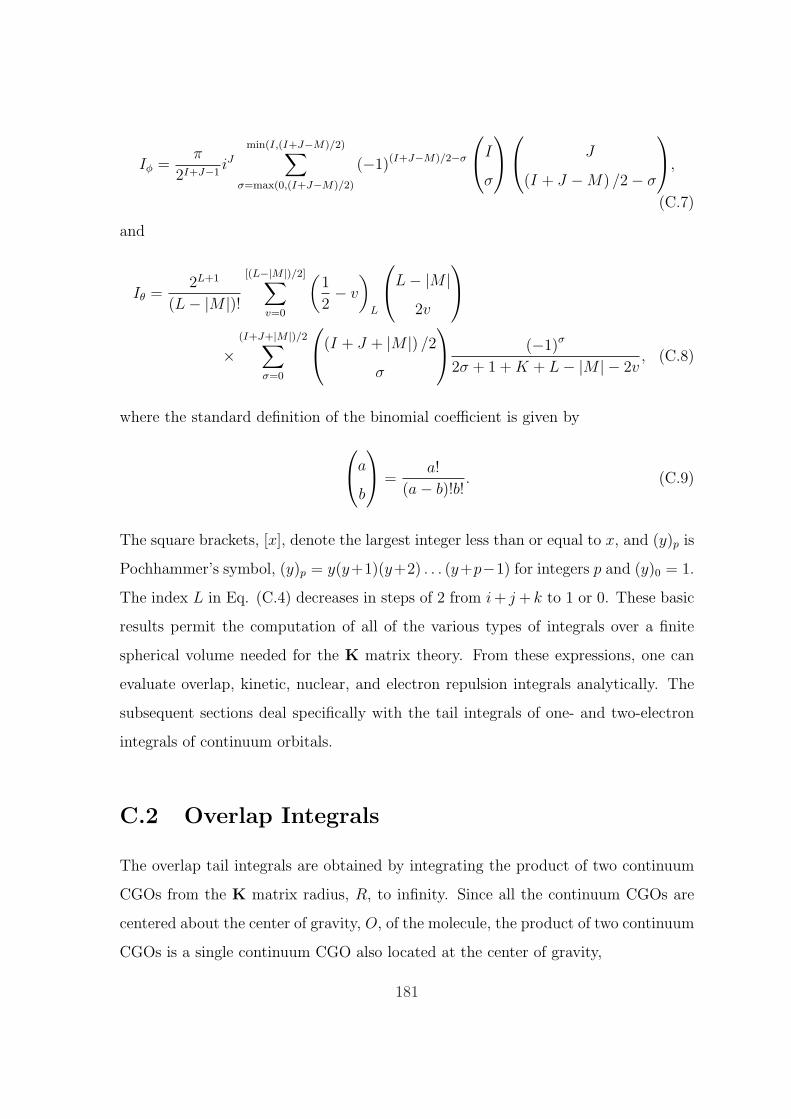
Iφ =π
2I+J−1iJ
min(I,(I+J−M)/2)∑
σ=max(0,(I+J−M)/2)
(−1)(I+J−M)/2−σ
I
σ
J
(I + J −M) /2− σ
,
(C.7)
and
Iθ =2L+1
(L− |M |)![(L−|M |)/2]∑
v=0
(1
2− v
)
L
L− |M |
2v
×(I+J+|M |)/2∑
σ=0
(I + J + |M |) /2
σ
(−1)σ
2σ + 1 + K + L− |M | − 2v, (C.8)
where the standard definition of the binomial coefficient is given by
a
b
=
a!
(a− b)!b!. (C.9)
The square brackets, [x], denote the largest integer less than or equal to x, and (y)p is
Pochhammer’s symbol, (y)p = y(y+1)(y+2) . . . (y+p−1) for integers p and (y)0 = 1.
The index L in Eq. (C.4) decreases in steps of 2 from i + j + k to 1 or 0. These basic
results permit the computation of all of the various types of integrals over a finite
spherical volume needed for the K matrix theory. From these expressions, one can
evaluate overlap, kinetic, nuclear, and electron repulsion integrals analytically. The
subsequent sections deal specifically with the tail integrals of one- and two-electron
integrals of continuum orbitals.
C.2 Overlap Integrals
The overlap tail integrals are obtained by integrating the product of two continuum
CGOs from the K matrix radius, R, to infinity. Since all the continuum CGOs are
centered about the center of gravity, O, of the molecule, the product of two continuum
CGOs is a single continuum CGO also located at the center of gravity,
181
χi,O (pi, qi, ri, ai) χj,O (pj, qj, rj, aj) = xpyqzre−ar2
, (C.10)
where p = pi + pj, q = qi + qj, r = ri + rj, and a = ai + aj. Since the product of
the two continuum CGOs is a Gaussian located at the center of gravity, RP = 0, the
following relations hold for this special case,
Apqrijk = δi,pδj,qδk,r, (C.11)
il (0) = δl,0. (C.12)
Therefore, the expression for the radial function reduces to the following
C lmpqra (r) = 4πe−ar2
rp+q+rY ∗0,0 (0)
∑L,M
BLMpqr 〈Yl,m|YL,M |Y0,0〉
= e−ar2
rp+q+r∑L,M
BLMpqr 〈Yl,m| YL,M〉
= e−ar2
rp+q+rBlmpqr.
(C.13)
The calculation of the overlap tail integral involves the integration of Eq. (C.2) from
R to infinity with the radial function given by Eq. (C.13)
Stail =∞∑
l=0
l∑
m=−l
∫ r=∞
r=R
e−ar2
rp+q+rBlmpqrYl,m (r) dr. (C.14)
After integration over the angular variables, one obtains
Stail =√
4πB00pqr
∫ ∞
R
rp+q+r+2e−ar2
dr
=√
πB00pqr
Γ [1/2 (p + q + r) + 3/2, aR2]
a1/2(p+q+r)+3/2.
(C.15)
182

C.3 Kinetic Energy Integrals
The kinetic energy tail integrals are defined by
KEtail = −1
2
∫ r=∞
r=R
χi,O (pi, qi, ri, ai)∇2χj,O (pj, qj, rj, aj) dr. (C.16)
The action of the kinetic energy operator on a continuum CGO centered about the
center of gravity O is given by
−1
2∇2
(xpyqzre−ar2
)= a [2 (p + q + r) + 3] xpyqzre−ar2
− 2a2[xp+2yqzr + xpyq+2zr + xpyqzr+2
]e−ar2
− 1
2
[p (p− 1) xp−2yqzr + q (q − 1) xpyq−2zr
+r (r − 1) xpyqzr−2]e−ar2
.
(C.17)
Let S (p, q, r, a) denote the overlap tail integral between χi (pi, qi, ri, ai) and
χj (pj, qj, rj, aj) where p = pi + pj, q = qi + qj, r = ri + rj, and a = ai + aj.
The kinetic energy tail integral is given by the sum of seven overlap tail integrals:
KEtail = aj [2 (pj + qj + rj) + 3] S (p, q, r, a)
− 2a2j [S (p + 2, q, r, a) + S (p, q + 2, r, a) + S (p, q, r + 2, a)]
− 1
2[pj (pj − 1) S (p− 2, q, r, a) + qj (qj − 1) S (p, q − 2, r, a)
+rj (rj − 1) S (p, q, r − 2, a)] ,
(C.18)
where the closed analytical forms for the seven different S integrals can be found from
Eq. (C.15).
C.4 Nuclear Attraction Integrals
For a nucleus centered about the point rC = (xC , yC , zC), the nuclear attraction tail
integral is given by
183
NAItail =
∫ r=∞
r=R
χi,O (pi, qi, ri, ai)1
|r− rC|χj,O (pj, qj, rj, aj) dr. (C.19)
Using Eqs. (C.10) and (C.13), the number of Gaussians involved in the integration
is reduced to one, and Eq. (C.19) takes the form
NAItail =∞∑
l=0
l∑
m=−l
Blmpqr
∫ r=∞
r=R
rp+q+re−ar2
Yl,m (r)1
|r− rC|dr. (C.20)
where p = pi + pj, q = qi + qj, r = ri + rj, and a = ai + aj. The Coulomb term can
be expressed using the well-known multipolar expansion,
1
|r− rC| = 4π∞∑
l=0
l∑
m=−l
1
2l + 1
rl<
rl+1>
Y ∗l,m (r) Yl,m (rc). (C.21)
Since the integration of Eq. (C.20) is from R to infinity and the K matrix radius
encloses all the nuclei, thus r> = r and r< = rC ; after integration over the angular
variables, one obtains
NAItail = 4π∞∑
l=0
l∑
m=−l
1
2l + 1rlCYl,m (rc) Blm
pqr
∫ ∞
R
rp+q+r−l+1e−ar2
dr. (C.22)
Since the index l in Eq. (C.22) decreases by steps of 2 from p + q + r to 1 or 0, the
exponent of r in the integral is always positive. Therefore
NAItail = 2π
p+q+r∑
l=0,1
l∑
m=−l
1
2l + 1rlCYl,m (rc) Blm
pqr
Γ [1/2 (p + q + r − l) + 1, aR2]
a1/2(p+q+r−l)+1,
rC 6= 0. (C.23)
Note that the original sum in Eq. (C.20) is finite because it is limited by the coefficient
Blmijk in Eq. (C.23). However, Eq. (C.23) is not applicable when a continuum CGO
is centered about a nucleus located at the center of gravity of the molecule (i.e., this
occurs in the equilibrium linear geometries of CO2 or NO+2 ). In this special case, the
184
Coulomb term is simply 1/r, and Eq. (C.20) reduces to
NAItail =∞∑
l=0
l∑
m=−l
Blmpqr
∫ r=∞
r=R
rp+q+r−1e−ar2
Yl,m (r) dr. (C.24)
After integration over the angular variables, one obtains
NAItail =√
4πB00pqr
∫ ∞
R
rp+q+r+1e−ar2
dr
=√
4πB00pqr
Γ [1/2 (p + q + r) + 1, aR2]
a1/2(p+q+r)+1, rC = 0.
(C.25)
C.5 Electron Repulsion Integrals
A general electron repulsion integral, evaluated over all space is given by
ERI =
∫ ∫χi,A1 (pi, qi, ri, ai) χj,B1 (pj, qj, rj, aj)
1
|r1 − r2|× χk,C2 (pk, qk, rk, ak) χl,D2 (pl, ql, rl, al) dr1dr2, (C.26)
where χi,Pn is the ith unnormalized Cartesian Gaussian Orbital (CGO) for electron
n centered at point Rn,P = (Xn,P , Yn,P , Zn,P ). Since only one electron can occupy a
continuum orbital in K matrix theory, only the two-electron tail integrals where either
χi and χj are continuum orbitals or χk and χl are continuum orbitals are required.
The latter integral is given by
ERI =
∫ ∫χi,A1 (pi, qi, ri, ai) χj,B1 (pj, qj, rj, aj)
1
|r1 − r2|× χk,O2 (pk, qk, rk, ak) χl,O2 (pl, ql, rl, al) dr1dr2, (C.27)
where χi,A1 and χj,B1 are nucleus-centered CGOs, and χk,O2 and χl,O2 are continuum
CGOs located at the center of gravity. By definition, this integral over all space can
be expanded as
185
ERI =
∫ r1=R
r1=0
∫ r2=R
r2=0
χi,A1χj,B11
|r1 − r2|χk,O2χl,O2dr1dr2
+
∫ r1=R
r1=0
∫ r2=∞
r2=R
χi,A1χj,B11
|r1 − r2|χk,O2χl,O2dr1dr2
+
∫ r1=∞
r1=R
∫ r2=R
r2=0
χi,A1χj,B11
|r1 − r2|χk,O2χl,O2dr1dr2
+
∫ r1=∞
r1=R
∫ r2=∞
r2=R
χi,A1χj,B11
|r1 − r2|χk,O2χl,O2dr1dr2.
(C.28)
However, only the tail integral is required. If the nucleus-centered CGOs are assumed
to have negligible contribution outside the K matrix radius, the only contribution to
the tail integral is
ERItail =
∫ r1=R
r1=0
∫ r2=∞
r2=R
χi,A1 (pi, qi, ri, ai) χj,B1 (pj, qj, rj, aj)1
|r1 − r2|χk,O2 (pk, qk, rk, ak) χl,O2 (pl, ql, rl, al) dr1dr2. (C.29)
Using the multipolar expansion,
1
|r1 − r2| = 4π∞∑
l=0
l∑
m=−l
1
2l + 1
rl<
rl+1>
Y ∗l,m (r1) Yl,m (r2)
= 4π∞∑
l=0
l∑
m=−l
1
2l + 1
1
r2l+1>
rl1Y
∗l,m (r1) rl
2Yl,m (r2).
(C.30)
From Eq. (C.29) one can identify r> = r2 and r< = r1; therefore,
ERItail
= 4π∞∑
l′=0
l′∑
m′=−l′
1
2l′ + 1
[∫ r1=R
r1=0
rl′1 Y ∗
l′,m′ (r1) χi,A1 (pi, qi, ri, ai) χj,B1 (pj, qj, rj, aj) dr1
×∫ r2=∞
r2=R
1
rl′+12
Yl′,m′ (r2) χk,O2 (pk, qk, rk, ak) χl,O2 (pl, ql, rl, al) dr2
]. (C.31)
186

Since the nucleus-centered CGOs are assumed to have negligible amplitude outside
the K matrix radius, the range of integration over r1 can be extended to all space
ERItail
= 4π∞∑
l′=0
l′∑
m′=−l′
1
2l′ + 1
[∫ r1=∞
r1=0
rl′1 Y ∗
l′,m′ (r1) χi,A1 (pi, qi, ri, ai) χj,B1 (pj, qj, rj, aj) dr1
×∫ r2=∞
r2=R
1
rl′+12
Yl′,m′ (r2) χk,O2 (pk, qk, rk, ak) χl,O2 (pl, ql, rl, al) dr2
]. (C.32)
First, consider the integration over r2. Using Eqs. (C.10) and (C.13), the number of
Gaussians involved in this integration is reduced to one and
∫ r2=∞
r2=R
1
rl′+12
Yl′,m′ (r2) χk,O2 (pk, qk, rk, ak) χl,O2 (pl, ql, rl, al) dr2
=∞∑
l′′=0
l′′∑
m′′=−l′′Bl′′m′′
pqr
∫ r2=∞
r2=R
rp+q+r−l′−12 e−ar2
2Yl′,m′ (r2) Yl′′,m′′ (r2) dr2, (C.33)
where p = pk + pl, q = qk + ql, r = rk + rl, and a = ak + al. After integration over the
angular variables, one obtains
∫ r2=∞
r2=R
1
rl′+12
Yl′,m′ (r2) χk,O2 (pk, qk, rk, ak) χl,O2 (pl, ql, rl, al) dr2
= Bl′m′∗pqr
∫ ∞
R
rp+q+r−l′+12 e−ar2
2dr2
= Bl′m′∗pqr
Γ [1/2 (p + q + r − l′) + 1, aR2]
2a1/2(p+q+r−l′)+1.
(C.34)
Now consider the integration over r1. Since the range of integration is over all space,
it is easiest to calculate this integral using Cartesian coordinates. The transformation
from Cartesian functions to spherical harmonic functions [161] is given by
rlYl,m (r) =∑
lx+ly+lz=l
c (l, m, lx, ly, lz) xlxylyzlz , (C.35)
where the complex constant c (l, m, lx, ly, lz) for unnormalized CGOs with m > 0 is
given by
187

c (l, m, lx, ly, lz)
= (−1)m
√(2l + 1) (l − |m|)!
4π (l + |m|)!1
2ll!
×(l−|m|)/2∑
i=0
l
i
i
(lx + ly − |m|) /2
(−1)i (2l − 2i)!
(l − |m| − 2i)!
×(lx+ly−|m|)/2∑
k=0
(lx + ly − |m|) /2
k
|m|
lx − 2k
(−1)(|m|−lx+2k)/2 ,
(C.36)
which is modified from Schlegel and Frisch’s original normalized expression to follow
the phase choice for m > 0. The transformation to Cartesian functions for m < 0 is
obtained using the phase choice given in Eq. (C.3).
The following identity will be very helpful in simplifying all further calculations:
χi,A (0, 0, 0, ai) χj,B (0, 0, 0, aj) = e−air2Ae−ajr2
B
= e−aiaj(A−B)2
ai+aj e−(ai+aj)r2P ,
(C.37)
where
rP = r−P = r− aiA + ajB
ai + aj
. (C.38)
It is also helpful to express Eq. (C.35) in terms of the Cartesian components of rP:
rlYl,m (r) =∑
lx+ly+lz=l
c (l, m, lx, ly, lz) (xP + Px)lx (yP + Py)
ly (zP + Pz)lz , (C.39)
where xP = x − Px, yP = y − Py, and zP = z − Pz. Using Eqs. (C.37) and (C.39),
the integral over r1 is given by
188

∫ r1=∞
r1=0
rl′1 Y ∗
l′,m′ (r1) χi,A1 (pi, qi, ri, ai) χj,B1 (pj, qj, rj, aj) dr1
= e−aiaj(A1−B1)2
ai+aj
∑
lx+ly+lz=l′c∗ (l′,m′, lx, ly, lz)
×∫ ∞
−∞
∫ ∞
−∞
∫ ∞
−∞(xP1 + P1x)
lx (yP1 + P1y)ly (zP1 + P1z)
lz
× xpi
A1yqi
A1zriA1x
pj
B1yqj
B1zrj
B1e−(ai+aj)x
2P1e−(ai+aj)y
2P1e−(ai+aj)z
2P1dx1dy1dz1.
(C.40)
The analysis is simpler if the other Cartesian components are also expressed in terms
of rP. For example,
xA1 = x− A1x = (x− P1x) + (P1x − A1x) = xP1 + PA1x, (C.41)
where PA1x ≡ P1x − A1x. Therefore
∫ r1=∞
r1=0
rl′1 Y ∗
l′,m′ (r1) χi,A1 (pi, qi, ri, ai) χj,B1 (pj, qj, rj, aj) dr1
= e−aiaj(A1−B1)2
ai+aj
∑
lx+ly+lz=l′c∗ (l′,m′, lx, ly, lz)
×∫ ∞
−∞
∫ ∞
−∞
∫ ∞
−∞(xP1 + P1x)
lx (yP1 + P1y)ly (zP1 + P1z)
lz
× (xP1 + PA1x)pi (yP1 + PA1y)
qi (zP1 + PA1z)ri
× (xP1 + PB1x)pj (yP1 + PB1y)
qj (zP1 + PB1z)rj
× e−(ai+aj)x2P1e−(ai+aj)y
2P1e−(ai+aj)z
2P1dx1dy1dz1.
(C.42)
The notation of Eq. (C.42) can be condensed further and rewritten as
189

∫ r1=∞
r1=0
rl′1 Y ∗
l′,m′ (r1) χi,A1 (pi, qi, ri, ai) χj,B1 (pj, qj, rj, aj) dr1
= e−aiaj(A1−B1)2
ai+aj
∑
lx+ly+lz=l′c∗ (l′,m′, lx, ly, lz)
×∫ ∞
−∞
∫ ∞
−∞
∫ ∞
−∞
lx+pi+pj∑α=0
fα (lx, pi, pj, P1x, PA1x, PB1x) xαP1e
−(ai+aj)x2P1
×ly+qi+qj∑
β=0
fβ (ly, qi, qj, P1y, PA1y, PB1y) yβP1e
−(ai+aj)y2P1
×lz+ri+rj∑
γ=0
fγ (lz, ri, rj, P1z, PA1z, PB1z) zγP1e
−(ai+aj)z2P1dx1dy1dz1,
(C.43)
where fα (lx, pi, pj, P1x, PA1x, PB1x) is the coefficient of xαP1 in the expansion
(xP1 + P1x)lx (xP1 + PA1x)
pi (xP1 + PB1x)pj . This coefficient is given by
fα (lx, pi, pj, P1x, PA1x, PB1x)
=a+b+c=α∑
a=0,lx
∑
b=0,pi
∑c=0,pj
P1lx−ax
lx
a
PA1pi−b
x
pi
b
PB1pj−c
x
pj
c
. (C.44)
Expressions for the other Cartesian components are similar. By symmetry, only the
even powers of xP1, yP1, and zP1 give nonzero contributions to the integral. The
following integral is useful
∫ ∞
−∞x2ne−αx2
dx =(2n− 1)!!
(2α)n
√π
α, (C.45)
where n is a positive integer. The integral over r1 becomes
190
∫ r1=∞
r1=0
rl′1 Y ∗
l′,m′ (r1) χi,A1 (pi, qi, ri, ai) χj,B1 (pj, qj, rj, aj) dr1
=
(π
ai + aj
)3/2
e−aiaj(A1−B1)2
ai+aj
∑
lx+ly+lz=l′c∗ (l′,m′, lx, ly, lz)
×[(lx+pi+pj)/2]∑
α=0
f2α (lx, pi, pj, P1x, PA1x, PB1x)(2α− 1)!!
[2 (ai + aj)]α
×[(ly+qi+qj)/2]∑
β=0
f2β (ly, qi, qj, P1y, PA1y, PB1y)(2β − 1)!!
[2 (ai + aj)]β
×[(lz+ri+rj)/2]∑
γ=0
f2γ (lz, ri, rj, P1z, PA1z, PB1z)(2γ − 1)!!
[2 (ai + aj)]γ .
(C.46)
Note that Eq. (C.32) is finite because it is limited by the coefficient Blmijk in Eq.
(C.34). Thus, the electron repulsion tail integral is given by summations over the
product of Eqs. (C.34) and (C.46).
191

192
Bibliography
[1] P. Dupre, R. Jost, M. Lombardi, P. G. Green, E. Abramson, and R. W. Field.
Chem. Phys., 152:293, 1991.
[2] G. Staszewska and L. Wolniewicz. J. Mol. Spectrosc., 212:208, 2002.
[3] M. Arif, Ch. Jungen, and A. L. Roche. J. Chem. Phys., 106:4102, 1997.
[4] B. Yoo and C. H. Greene. Phys. Rev. A, 34:1635, 1986.
[5] Y. Chuang and D. G. Truhlar. J. Chem. Phys., 112:1221, 2000.
[6] J. K. G. Watson. Mol. Phys., 15:479, 1968.
[7] B. M. Wong, R. L. Thom, and R. W. Field. J. Phys. Chem. A, 110:7406, 2006.
[8] J. T. Hougen, P. R. Bunker, and J. W. C. Johns. J. Mol Spectrosc., 34:136,
1970.
[9] D. P. Tew, N. C. Handy, and S. Carter. Mol. Phys., 99:393, 2001.
[10] B. M. Wong, A. H. Steeves, and R. W. Field. J. Phys. Chem. B, 110:18912,
2006.
[11] C. Eckart. Phys. Rev., 47:552, 1935.
[12] D. P. Tew, N. C. Handy, S. Carter, S. Irle, and J. Bowman. Mol. Phys., 101:3513,
2003.
[13] W. H. Miller, N. C. Handy, and J. E. Adams. J. Chem. Phys., 72:99, 1980.
193
[14] K. N. Rao and C. W. Mathews. Molecular Spectroscopy: Modern Research.
Academic Press: New York, 1972.
[15] E. B. Wilson Jr., J. C. Decius, and P. C. Cross. Molecular Vibrations: The
Theory of Infrared and Raman Vibrational Spectra. Dover Publications: New
York, 1955.
[16] C. C. Lin and J. D. Swalen. Rev. Mod. Phys., 31:841, 1959.
[17] P. Rabinowitz. Numerical Methods for Nonlinear Algebraic Equations. Gordon
and Breach Science Publishers: New York, 1970.
[18] http://www.mathworks.com/matlabcentral/fileexchange
/loadFile.do?objectId=14240&objectType=FILE.
[19] K. S. Pitzer and W. D. Gwinn. J. Chem. Phys., 10:428, 1942.
[20] K. S. Pitzer. J. Chem. Phys., 14:239, 1946.
[21] K. S. Pitzer and J. E. Kilpatrick. J. Chem. Phys., 17:1064, 1949.
[22] A. L. L. East and L. Radom. J. Chem. Phys., 106:6655, 1997.
[23] L. S. Kassel. J. Chem. Phys., 4:276, 1936.
[24] B. L. Crawford Jr. J. Chem. Phys., 8:273, 1940.
[25] M. J. Frisch, G. W. Trucks, H. B. Schlegel, G. E. Scuseria, M. A. Robb, J. R.
Cheeseman, J. A. Montgomery, Jr., T. Vreven, K. N. Kudin, J. C. Burant, J. M.
Millam, S. S. Iyengar, J. Tomasi, V. Barone, B. Mennucci, M. Cossi, G. Scal-
mani, N. Rega, G. A. Petersson, H. Nakatsuji, M. Hada, M. Ehara, K. Toy-
ota, R. Fukuda, J. Hasegawa, M. Ishida, T. Nakajima, Y. Honda, O. Kitao,
H. Nakai, M. Klene, X. Li, J. E. Knox, H. P. Hratchian, J. B. Cross, V. Bakken,
C. Adamo, J. Jaramillo, R. Gomperts, R. E. Stratmann, O. Yazyev, A. J.
Austin, R. Cammi, C. Pomelli, J. W. Ochterski, P. Y. Ayala, K. Morokuma,
G. A. Voth, P. Salvador, J. J. Dannenberg, V. G. Zakrzewski, S. Dapprich, A. D.
194

Daniels, M. C. Strain, O. Farkas, D. K. Malick, A. D. Rabuck, K. Raghavachari,
J. B. Foresman, J. V. Ortiz, Q. Cui, A. G. Baboul, S. Clifford, J. Cioslowski,
B. B. Stefanov, G. Liu, A. Liashenko, P. Piskorz, I. Komaromi, R. L. Martin,
D. J. Fox, T. Keith, M. A. Al-Laham, C. Y. Peng, A. Nanayakkara, M. Chal-
lacombe, P. M. W. Gill, B. Johnson, W. Chen, M. W. Wong, C. Gonzalez, and
J. A. Pople. Gaussian 03, Revision D.01. Gaussian, Inc., Wallingford, CT, 2004.
[26] L. A. Curtiss, K. Raghavachari, P. C. Redfern, V. Rassolov, and J. A. Pople.
J. Chem. Phys., 109:7764, 1998.
[27] P. Y. Ayala and H. B. Schlegel. J. Chem. Phys., 108:2314, 1998.
[28] A. Chung-Phillips. J. Comput. Chem., 13:874, 1992.
[29] Y. El Youssoufi, M. Herman, and J. Lievin. Mol. Phys., 94:461, 1998.
[30] V. Hnizdo, A. Fedorowicz, H. Singh, and E. Demchuk. J. Comput. Chem.,
24:1172, 2003.
[31] Y. El Youssoufi, R. Georges, J. Lievin, and M. Herman. J. Mol. Spectrosc.,
186:239, 1997.
[32] Y. El Youssoufi, J. Lievin, J. Vander Auwera, and M. Herman. Mol. Phys.,
94:473, 1998.
[33] S. Zou and J. M. Bowman. Chem. Phys. Lett., 368:421, 2003.
[34] S. Zou, J. M. Bowman, and A. Brown. J. Chem. Phys., 118:10012, 2003.
[35] L. Liu and J. T. Muckerman. J. Chem. Phys., 107:3402, 1997.
[36] D. Xu, G. Li, D. Xie, and H. Guo. Chem. Phys. Lett., 365:480, 2002.
[37] D. Xu, R. Chen, and H. Guo. J. Chem. Phys., 118:7273, 2003.
[38] R. A. Kendall, T. H. Dunning Jr., and R. J. Harrison. J. Chem. Phys., 96:6796,
1992.
195

[39] M. P. Jacobson, J. P. O’Brien, R. J. Silbey, and R. W. Field. J. Chem. Phys.,
109:121, 1998.
[40] M. P. Jacobson, J. P. O’Brien, and R. W. Field. J. Chem. Phys., 109:3831,
1998.
[41] Matthew Paul Jacobson. Spectroscopic Patterns Encode Unimolecular Dynam-
ics. PhD thesis, Massachusetts Institute of Technology, 1999.
[42] Michelle Lee Silva. Spectroscopic Investigations of the X and A State Dynamics
of 13C2H2. PhD thesis, Massachusetts Institute of Technology, 2002.
[43] Zicheng Duan. Spectroscopic Study of the Acetylene Species. PhD thesis, Mas-
sachusetts Institute of Technology, 2003.
[44] R. L. Hayes, E. Fattal, N. Govind, and E. Carter. J. Am. Chem. Soc., 123:641,
2001.
[45] J. A. Bentley, R. E. Wyatt, M. Menou, and C. Leforestier. J. Chem. Phys.,
97:4255, 1992.
[46] J. F. Stanton and J. Gauss. J. Chem. Phys., 110:6079, 1999.
[47] J. F. Stanton and J. Gauss. J. Chem. Phys., 110:1831, 1999.
[48] M. P. Jacobson, R. J. Silbey, and R. W. Field. J. Chem. Phys., 110:845, 1999.
[49] L. Halonen, M. S. Child, and S. Carter. Mol. Phys., 47:1097, 1982.
[50] L. Halonen. Adv. Chem. Phys., 104:41, 1998.
[51] S. F. Yang, L. Halonen, and A. Campargue. Mol. Phys., 99:1303, 2001.
[52] G. J. Scherer, K. K. Lehmann, and W. Klemperer. J. Chem. Phys., 78:2817,
1983.
[53] K. K. Lehmann. J. Chem. Phys., 96:8117, 1992.
196

[54] R. Prosmiti and S. C. Farantos. J. Chem. Phys., 103:3299, 1995.
[55] R. Prosmiti and S. C. Farantos. J. Chem. Phys., 118:8275, 2003.
[56] J. P. Rose and M. E. Kellman. J. Chem. Phys., 105:10743, 1996.
[57] E. L. Sibert and A. B. McCoy. J. Chem. Phys., 105:469, 1996.
[58] J. A. Barnes, T. E. Gough, and M. Stoer. Chem. Phys. Lett., 237:437, 1995.
[59] J. A. Barnes, T. E. Gough, and M. Stoer. J. Chem. Phys., 114:4490, 2001.
[60] J. S. Muenter and V. W. Laurie. J. Am. Chem. Soc., 86:3901, 1964.
[61] K. Matsumura, T. Tanaka, Y. Endo, S. Saito, and E. Hirota. J. Phys. Chem.,
84:1793, 1980.
[62] J. M. Bowman, S. Irle, K. Morokuma, and A. Wodtke. J. Chem. Phys.,
114:7923, 2001.
[63] C. Jung, H. S. Taylor, and M. P. Jacobson. J. Phys. Chem. A, 105:681, 2001.
[64] S. Rainer and H. Koppel. J. Chem. Phys., 115:7907, 2001.
[65] M. Bittner and H. Koppel. Phys. Chem. Chem. Phys., 5:4604, 2003.
[66] V. Szalay. J. Mol. Spectrosc., 128:24, 1988.
[67] K. Fukui. J. Phys. Chem., 74:4161, 1970.
[68] K. Fukui. Acc. Chem. Chem. Phys., 14:363, 1981.
[69] Z. Bacic and J. C. Light. J. Chem. Phys., 85:4594, 1986.
[70] T. J. Lee and P. R. Taylor. Int. J. Quantum Chem., page 199, 1989.
[71] H.-J. Werner, P. J. Knowles, R. Lindh, F. R. Manby, M. Schutz, P. Celani,
T. Korona, G. Rauhut, R. D. Amos, A. Bernhardsson, A. Berning, D. L. Cooper,
M. J. O. Deegan, A. J. Dobbyn, F. Eckert, C. Hampel, G. Hetzer, A. W. Lloyd,
197

S. J. McNicholas, W. Meyer, M. E. Mura, A. Nicklass, P. Palmieri, R. Pitzer,
U. Schumann, H. Stoll, A. J. Stone, R. Tarroni, and T. Thorsteinsson. Molpro,
version 2002.6, a package of ab initio programs. See http://www.molpro.net,
Cardiff, UK, 2002.
[72] P. G. Szalay and R. J. Bartlett. Chem. Phys. Lett., 214:481, 1993.
[73] M. I. El Idrissi, J. Lievin, A. Campargue, and M. Herman. J. Chem. Phys.,
110:2074, 1999.
[74] K. Hoshina, A. Iwasaki, K. Yamanouchi, M. P. Jacobson, and R. W. Field. J.
Chem. Phys., 114:7424, 2001.
[75] M. A. Temsamani and M. Herman. J. Chem. Phys., 102:6371, 1995.
[76] M. A. Temsamani, M. Herman, S. A. B. Solina, J. P. O’Brien, and R. W. Field.
J. Chem. Phys., 105:11357, 1996.
[77] G. Strey and I. M. Mills. J. Mol. Spectrosc., 59:103, 1976.
[78] G. Hose and H. S. Taylor. J. Chem. Phys., 76:5356, 1982.
[79] P. L. Cummins, G. B. Bacskay, and N. S. Hush. J. Phys. Chem., 89:2151, 1985.
[80] H. B. G. Casimir. Archives du Musee Teyler (III), 8:201, 1936.
[81] B. T. Feld and W. E. Lamb Jr. Phys. Rev., 67:15, 1945.
[82] E. H. Rhoderick. Nature, 160:255, 1947.
[83] R. Pd and P. Chandra. J. Chem. Phys., 114:7450, 2001.
[84] A. G. Maki, G. Ch. Mellau, S. Klee, M. Winnewisser, and W. Quapp. J. Mol
Spectrosc., 202:67, 2000.
[85] A. G. Maki and G. Ch. Mellau. J. Mol Spectrosc., 206:47, 2001.
[86] H. A. Bechtel, A. H. Steeves, and R. W. Field. ApJ., 649:L53, 2006.
198

[87] R. L. Thom, B. M. Wong, R. W. Field, and J. F. Stanton. J. Chem. Phys.,
126:184307, 2007.
[88] P. Dupre and P. G. Green. Chem. Phys. Lett., 212:555, 1993.
[89] P. Dupre, P. G. Green, and R. W. Field. Chem. Phys., 196:211, 1995.
[90] P. Dupre. Chem. Phys., 196:239, 1995.
[91] G. Vacek, C. D. Sherrill, Y. Yamaguchi, and H. F. Schaefer III. J. Chem. Phys.,
104:1774, 1996.
[92] C. D. Sherrill, G. Vacek, Y. Yamaguchi, H. F. Schaefer III, J. F. Stanton, and
J. Gauss. J. Chem. Phys., 104:8507, 1996.
[93] Selen Altunata. Intersystem Crossing in Acetylene: A Mechanistic Study. PhD
thesis, Massachusetts Institute of Technology, 2001.
[94] Kevin Laughton Cunningham. The Surface Ejection of Electrons by Laser Ex-
cited Metastables Spectroscopy of Acetylene. PhD thesis, Massachusetts Insti-
tute of Technology, 2000.
[95] Ryan L. Thom. Spectroscopic Investigations of Intersystem Crossing and Triplet
State Structure in Acetylene. PhD thesis, Massachusetts Institute of Technology,
2006.
[96] A. P. Mishra, R. L. Thom, and R. W. Field. J. Mol. Spectrosc., 228:565, 2004.
[97] Q. Cui, K. Morokuma, and J. F. Stanton. Chem. Phys. Lett., 263:46, 1996.
[98] Q. Cui and K. Morokuma. Chem. Phys. Lett., 272:319, 1997.
[99] E. Ventura, M. Dallos, and H. Lischka. J. Chem. Phys., 118:1702, 2003.
[100] J. F. Stanton, J. Gauss, J. D. Watts, P. G. Szalay, and R. J. Bartlett. Aces2,
mainz-austin-budapest version, a quantum-chemical program package for high-
level calculations of energies and properties. See http://www.aces2.de.
199
[101] G. Orlandi and F. Zerbetto. J. Chem. Phys., 91:4238, 1987.
[102] G. Orlandi, F. Zerbetto, and M. Z. Zgierski. Chem. Rev., 91:867, 1991.
[103] H. C. Longuet-Higgins. Adv. Spectrosc., 2:42, 1961.
[104] R. L. Fulton and M. Gouterman. J. Chem. Phys., 35:1059, 1961.
[105] W. H. Henneker, A. P. Penner, W. Siebrand, and M. Z. Zgierski. J. Chem.
Phys., 69:1884, 1978.
[106] A. J. Merer, N. Yamakita, S. Tsuchiya, J. F. Stanton, Z. Duan, and R. W.
Field. Mol. Phys., 101:663, 2003.
[107] J. D. Tobiason, A. L. Utz, E. L. Sibert III, and F. F. Crim. J. Chem. Phys.,
99:5762, 1993.
[108] T. E. Sharp and H. M. Rosenstock. J. Chem. Phys., 41:3453, 1964.
[109] P. T. Ruhoff and M. A. Ratner. Int. J. Quant. Chem., 77:383, 2000.
[110] A. Toniolo and M. Persico. Int. J. Quant. Chem., 22:969, 2001.
[111] F. Duschinski. Acta Physikochim. URSS, 7:551, 1937.
[112] http://www.mathworks.com/matlabcentral/fileexchange
/loadFile.do?objectId=14992&objectType=FILE.
[113] I. M. Mills. Molecular Spectroscopy: Modern Research. Academic Press, 1972.
[114] B. M. Wong, S. N. Altunata, and R. W. Field. J. Chem. Phys., 124:014106,
2006.
[115] M. J. Seaton. Proc. Phys. Soc., 88:801, 1966.
[116] M. J. Seaton. Rep. Prog. Phys., 46:167, 1983.
[117] U. Fano. Phys. Rev. A, 2:353, 1970.
200
[118] Ch. Jungen. Molecular Applications of Quantum Defect Theory. IOP Publish-
ing: Bristol, 1996.
[119] C. H. Greene, A. R. P Rau, and U. Fano. Phys. Rev. A, 26:2441, 1982.
[120] S. Ross. An MQDT primer. In AIP Conference Proceedings No. 225, 1991.
[121] Serhan N. Altunata. Generalized Quantum Defect Methods in Quantum Chem-
istry. PhD thesis, Massachusetts Institute of Technology, 2006.
[122] P. G. Burke, I. Mackey, and I. Shimamura. J. Phys. B, 10:2497, 1977.
[123] S. E. Branchett and J. Tennyson. Phys. Rev. Lett., 64:2889, 1990.
[124] L. A. Morgan, C. J. Gillan, J. Tennyson, and X. Chen. J. Phys. B, 30:4087,
1997.
[125] S. F. Boys. Proc. R. Soc. London, Ser. A, 200:542, 1950.
[126] H. Taketa, S. Huzinaga, and K. O-ohata. J. Phys. Soc. Jpn., 21:2313, 1966.
[127] E. F. Valeev and H. F. Schaefer III. J. Chem. Phys., 113:3990, 2000.
[128] E. F. Valeev and C. L. Janssen. J. Chem. Phys., 121:1214, 2004.
[129] T. D. Crawford, S. S. Wesolowski, E. F. Valeev, R. A. King, M. L. Leininger,
and H. F. Schaefer III. Chemistry for the 21st Century. Wiley-VCH: Weinheim,
2001.
[130] M. Head-Gordon and J. A. Pople. J. Chem. Phys., 89:5777, 1988.
[131] T. D. Crawford, C. D. Sherrill, E. F. Valeev, J. T. Fermann, R. A. King, M. L.
Leininger, S. T. Brown, C. L. Janssen, E. T. Seidl, J. P. Kenny, and W. D.
Allen. J. Comput. Chem., 28:1610, 2007.
[132] A. Faure, J. D. Gorfinkiel, L. A. Morgan, and J. Tennyson. Comput. Phys.
Commun., 114:224, 2002.
201

[133] W. M. Huo and F. A. Gianturco. Computational Methods for Electron-Molecule
Collisions. Plenum Press: New York, 1995.
[134] M. Yoshimine. J. Comput. Phys., 11:449, 1969.
[135] A. Szabo and N. S. Ostlund. Modern Quantum Chemistry: Introduction to
Advanced Electronic Structure Theory. Dover Publications: New York, 1996.
[136] C. J. Noble, P. G. Burke, and S. Salvini. J. Phys. B, 15:3779, 1982.
[137] J. Tennyson, C. J. Noble, and S. Salvini. J. Phys. B, 17:905, 1984.
[138] J. Tennyson, C. J. Noble, and S. Salvini. J. Phys. B, 29:6185, 1984.
[139] P. G. Burke, C. J. Noble, and P. Scott. Proc. R. Soc. Lond. A, 410:289, 1987.
[140] J. Tennyson, P. G. Burke, and K. A. Berrington. Comput. Phys. Commun.,
47:207, 1987.
[141] J. Tennyson. J. Phys. B, 29:1817, 1996.
[142] H. J. Monkhorst. Int. J. Quantum Chem. Sym., 11:421, 1977.
[143] S. Ghosh and D. Mukherjee. Proc. Indian Acad. Sci., 93:947, 1984.
[144] J. Geertsen, M. Rittby, and R. J. Bartlett. Chem. Phys. Lett., 164:57, 1989.
[145] H. Koch and P. Jørgensen. J. Chem. Phys., 93:3333, 1990.
[146] J. Verges, C. Effantin, A. Bernard, A. Topouzkhanian, A. R. Allouche,
J. D’Incan, and R. F. Barrow. J. Phys. B, 26:279, 1993.
[147] A. Bernard, C. Effantin, E. Andrianavalona, J. Verges, and R. F. Barrow. J.
Mol. Spectrosc., 152:174, 1992.
[148] J. E. Murphy, J. M. Berg, A. J. Merer, N. A. Harris, and R. W. Field. Phys.
Rev. Lett., 65:1861, 1990.
[149] Z. J. Jakubek and R. W. Field. Phys. Rev. Lett., 72:2167, 1994.
202
[150] N. A. Harris and Ch. Jungen. Phys. Rev. Lett., 70:2549, 1993.
[151] M. A. Iron, M. Oren, and J. M. L. Martin. Mol. Phys., 101:1345, 2003.
[152] D. J. Griffiths. Introduction to Electrodynamics. Prentice Hall: New Jersey,
1989.
[153] M. Aubert, N. Bessis, and G. Bessis. Phys. Rev. A, 10:51, 1974.
[154] Ch. Jungen and F. Texier. J. Phys. B, 33:2495, 2000.
[155] A. Matzkin. Phys. Rev. A, 63:012103, 2001.
[156] K. E. Thylwe and H. J. Korsch. J. Phys. A, 34:3497, 2001.
[157] M. Hiyama and M. S. Child. J. Phys. B, 34:3935, 2001.
[158] A. Matzkin and M. Lombardi. Phys. Rev. E, 66:037702, 2002.
[159] H. Le Rouzo. Int. J. Quant. Chem., 64:647, 1997.
[160] R. J. Mathar. Int. J. Quant. Chem., 90:227, 2002.
[161] H. Schlegel and M. J. Frisch. Int. J. Quant. Chem., 54:83, 1995.
203

Curriculum Vitae
BIRTH DATE: August 3, 1979.
EDUCATION: Rice University, B.S. (2001);Massachusetts Institute of Technology, Ph.D. (2007).
PUBLICATIONS:
Bryan M. Wong, Maria M. Fadri, and Sumathy Raman. “Thermodynamic Calcu-lations for Molecules with Asymmetric Internal Rotors II – Application to the 1,2-Dihaloethanes.” Journal of Computational Chemistry, 28, in press, (2007).
Ryan L. Thom, Bryan M. Wong, Robert W. Field, and John F. Stanton. “Stud-ies of Intersystem Crossing Dynamics in Acetylene.” Journal of Chemical Physics,126, 184307-1–184307-7, (2007).
Bryan M. Wong and Sumathy Raman. “Thermodynamic Calculations for Moleculeswith Asymmetric Internal Rotors – Application to the 1,3-Butadiene.” Journal ofComputational Chemistry, 28, 759–766, (2007).
Bryan M. Wong, Adam H. Steeves, and Robert W. Field. “Electronic Signaturesof Large Amplitude Motions: Dipole Moments of Vibrationally Excited Local-Bendand Local-Stretch States of S0 Acetylene.” Journal of Physical Chemistry B, 110,18912–18920, (2006).
Bryan M. Wong, Ryan L. Thom, and Robert W. Field. “Accurate Inertias for Large-Amplitude Motions: Improvements on Prevailing Approximations.”Journal of Phys-ical Chemistry A, 110, 7406–7413, (2006).
Bryan M. Wong, Serhan N. Altunata, and Robert W. Field. “Analytical Calcula-tions of Molecular Integrals for Multielectron R-Matrix Methods.” Journal of Chem-ical Physics, 124, 014106-1–014106-9, (2006).
INTERESTS: Alumni interviewer for Rice University admissions; Classical violin-ist; Enjoys New England clam chowder; Has a sister who once won a strawberryeating contest in Illinois.
204