Lecture – 4

TITLE: Quantization of radiation and matter: Wave-Particle duality

Objectives

In this lecture, we will discuss the development of quantization of matter and light.

We will understand the need for quantum mechanics for describing the light matter interaction in the

microscopic level.

We will find the microscopic region where the wave particle duality is valid and application of

uncertainty principle in this regard.

We also find the development of famous Schrodinger equation to describe the quantization of

energy levels of atoms.

Page-1

In the last two lectures, we have gone through the chronological development of thoughts to understand

the matter (atom & molecules) and the radiation (light).

The motion of the matter in macroscopic domain (dimension 410 cm ) and the nature of light

as wave are completely described by Classical Physics.

In classical Physics,

(i) The events around us can be observed and directly measured with instruments.

(ii) There is a close link between our perception and the explanation.

(iii) For any dynamical physical system its state can be determined with the knowledge of its initial

state.

(iv) The matter (macroscopic quantity) is treated as localized entity with the state having defined

positions and velocities at any instant of time. So, the matter is having “particle nature” and

follows the Newtonian Mechanics.

(v) Radiation/light is treated as classical electromagnetic wave developed by Maxwell. This is the

kind of wave nature of light.

Page-2

Maxwell’s Equations are:

0

0 0 0

'

0

'

'

E Gauss s Law

B

BE Faraday s Law

t

EB J Ampere s Law

t

Equation – 4.1

where, E & B are the electric and magnetic field components;

is the charge density;

0 & 0 are the permeability and permittivity of the free space respectively;

and 0 0 2

1

c

In free space, i.e. no charge and current, Maxwell’s equations become,

2

0 ;

10 ;

BE E

t

EB B

c t

Equation – 4.2

Page-3

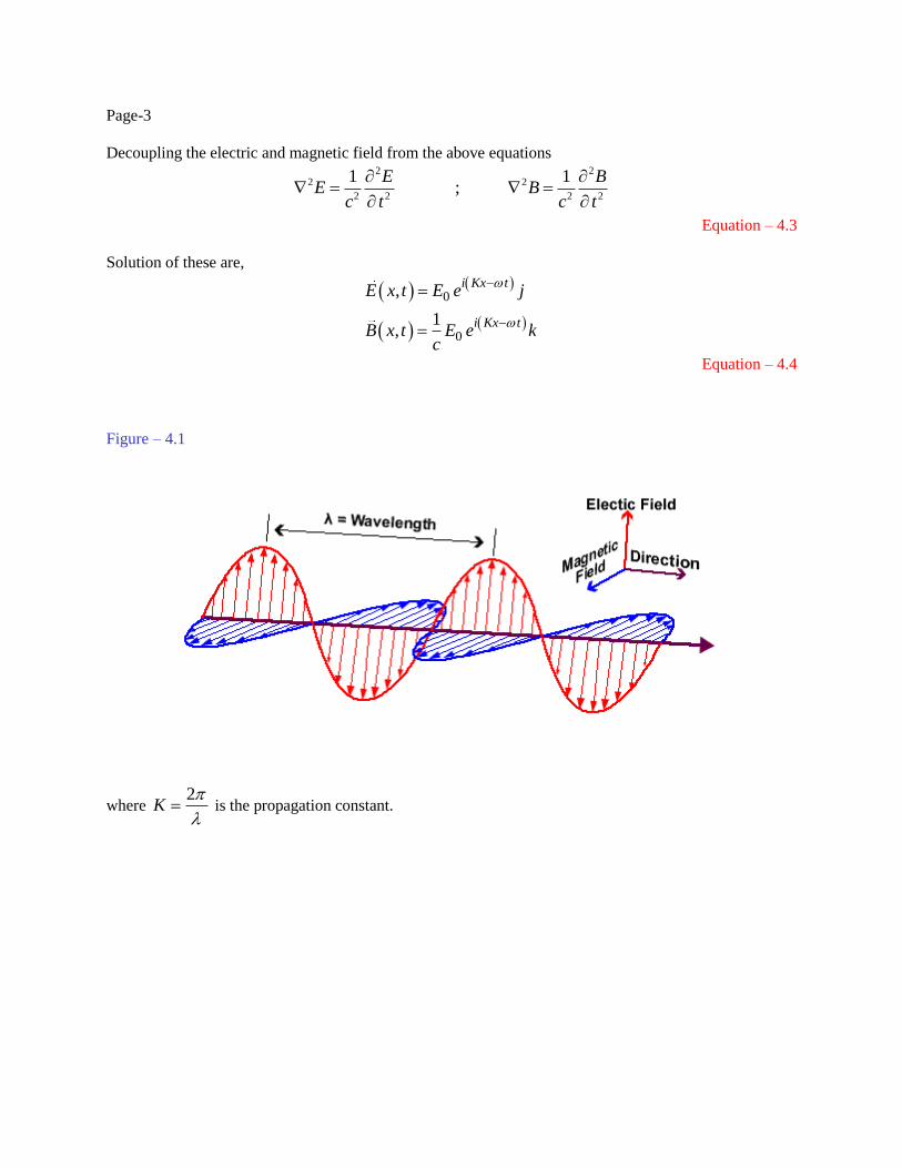
Decoupling the electric and magnetic field from the above equations 2 2

2 2

2 2 2 2

1 1;

E BE B

c t c t

Equation – 4.3

Solution of these are,

0

0

,

1,

i Kx t

i Kx t

E x t E e j

B x t E e kc

Equation – 4.4

Figure – 4.1

where 2

K

is the propagation constant.

Page-4

In the beginning of the 20th century, several experiments and observations could not be explained by

Classical Physics. These are

(i) Photoelectric effect

(ii) Compton effect

(iii) Phenomena on atomic scales such as classical explanation of Rutherford model, discrete energy levels

of atoms proposed by Bohr.

These facts forced the scientist to search for a near explanation of the mechanics.

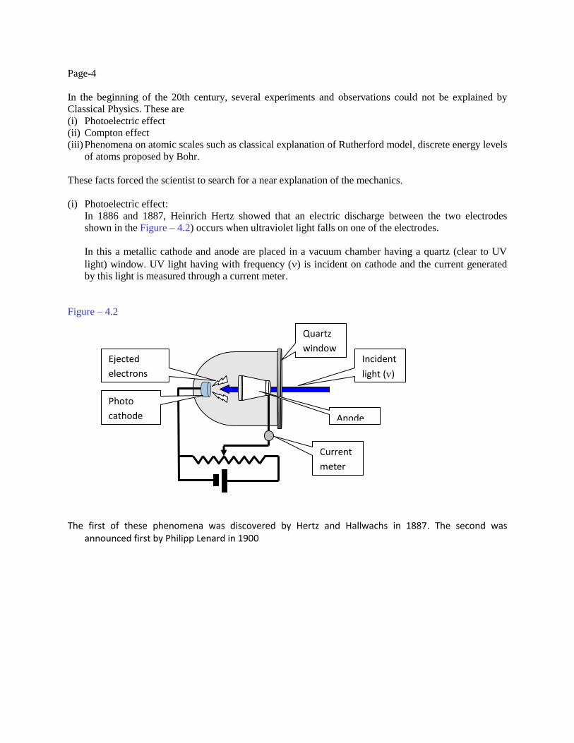
(i) Photoelectric effect:

In 1886 and 1887, Heinrich Hertz showed that an electric discharge between the two electrodes

shown in the Figure – 4.2) occurs when ultraviolet light falls on one of the electrodes.

In this a metallic cathode and anode are placed in a vacuum chamber having a quartz (clear to UV

light) window. UV light having with frequency () is incident on cathode and the current generated

by this light is measured through a current meter.

Figure – 4.2

The first of these phenomena was discovered by Hertz and Hallwachs in 1887. The second was announced first by Philipp Lenard in 1900

Quartz

window Incident

light ()

Anode

Current

meter

Photo

cathode

Ejected

electrons

Page – 5

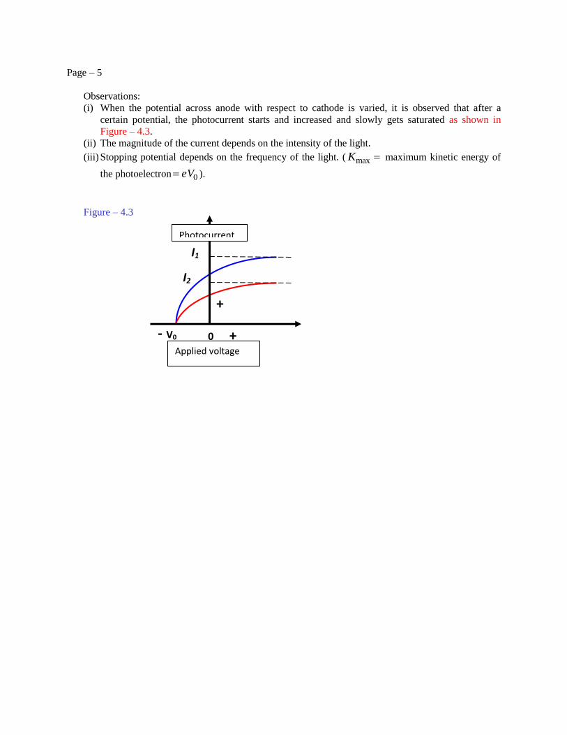
Observations:

(i) When the potential across anode with respect to cathode is varied, it is observed that after a

certain potential, the photocurrent starts and increased and slowly gets saturated as shown in

Figure – 4.3.

(ii) The magnitude of the current depends on the intensity of the light.

(iii) Stopping potential depends on the frequency of the light. ( maxK maximum kinetic energy of

the photoelectron 0eV ).

Figure – 4.3

Applied voltage

+ 0 - V0

+

I1

I2

Photocurrent

Page-6

These observations cannot be explained by classical theory. The reasons are

(i) In the wave picture, the amplitude of the electric field 0E (Figure - 4.1) increases as the light

intensity is increased. The force exerted by this electric field on the electron is e E . It means the

kinetic energy of the ejected photoelectron should increase if the intensity is increased. However,

from the figure, it is clear that max 0K eV which is independent of light intensity.

(ii) According to the wave theory, photoelectron should exit at any frequency of light if the exerted

force is greater than the binding force. However, observation is such that the photoelectrons for a

particular metal (cathode) are ejected only when the light frequency is greater than a particular

value, a cut off frequency 0 .

To overcome these discrepancies, Einstein took the idea given by Planck and assumed, that

The light energy is a bundle of energy localized in a small volume of space.

It remains localized even it moves with a velocity of light c. He termed the content of the

energy E as “PHOTON”, and is related to the frequency as given in Equation – 4.5.

E h

Equation – 4.5

For the photoelectric effect, he assumed that one of such photons is completely absorbed by

one electron of the photocathode as if particle-particle interaction and derived the kinetic

energy of the electron as given in Equation – 4.6.

0K h W

Equation – 4.6

where, 0W is the work functions of the photocathode.

Page-7

The particle nature of light (quantization of radiation) was again realized to explain the

Compton’s experiment in 1923.

The X-ray of wavelength 0 was incident on a target. With a crystal diffractometer, the

wavelengths of the scattered X-ray were measured by changing the angle .

Figure – 4.4

The scattered radiation consists of the primary wavelength 0 and a shifted wavelength .

The Compton shift 0 varies with the scattering angle.

The classical theory predicts that if the radiation of wavelength incidents on a particle, it

scatters and emits radiation of the same wavelength . No other wavelength is predicted by

this theory.

Using the particle nature of the radiation, from the momentum and energy

conservation, the Compton equation is derived to explain the observation as in

Equation – 4.7,

0

1 cos 1 cosc

h

m c

Equation – 4.7

where, o

12

0

2.43 10 0.0243Ac

hmeter

m c

Details are discussed in the next lecture.

X-Ray

source

Scatter

(electron)

Incident

beam

Scattered

beam

Crystal

(wavelength

selector)

Scattering

angle ()

Collimating

system

Detector

Page-8

Dual Nature of electromagnetic radiation

To describe the Compton observation, we need to treat radiation as localized particle, “Photon”. Here,

the radiation and matter interaction is particle-particle in nature.

Wave picture is indeed required to explain interference, diffraction phenomena.

In Compton’s experiment, the particle nature is used for the description of scattering. On the other

hand, the crystal is used to separate the wavelengths and this is based on diffraction (wave nature).

Electromagnetic radiation behaves wavelike under some circumstances and particle like under other

circumstances. Both pictures cannot be used simultaneously.

This wave particle dual nature not only exists for radiation. In fact subatomic particles also follow the

same.

Page-9

Matter Waves :

In 1924, Louis de Broglie first proposed the existence of matter waves.

He supported the wave-particle dual nature of radiation and proposed the existence of matter

waves. In his hypothesis, he suggested that the wave aspect of the matter is related to its particle nature in

the same quantitative way that is in case of radiation.

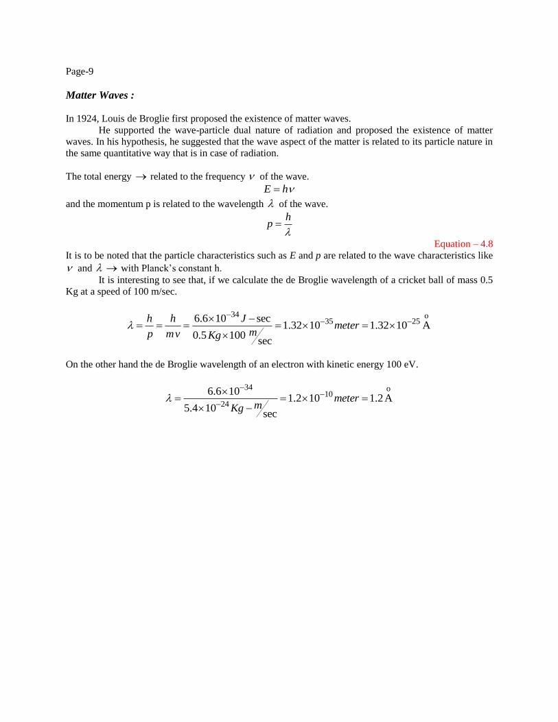
The total energy related to the frequency of the wave.

E h

and the momentum p is related to the wavelength of the wave.

hp

Equation – 4.8

It is to be noted that the particle characteristics such as E and p are related to the wave characteristics like

and with Planck’s constant h.

It is interesting to see that, if we calculate the de Broglie wavelength of a cricket ball of mass 0.5

Kg at a speed of 100 m/sec.

34 o

35 256.6 10 sec1.32 10 1.32 10 A

0.5 100sec

h h Jmeter

mp mv Kg

On the other hand the de Broglie wavelength of an electron with kinetic energy 100 eV.

34 o

10

24

6.6 101.2 10 1.2A

5.4 10sec

metermKg

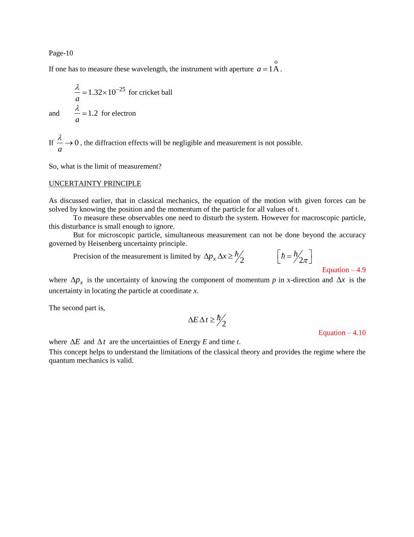
Page-10

If one has to measure these wavelength, the instrument with aperture o

1Aa .

251.32 10

a

for cricket ball

and 1.2a

for electron

If 0a

, the diffraction effects will be negligible and measurement is not possible.

So, what is the limit of measurement?

UNCERTAINTY PRINCIPLE

As discussed earlier, that in classical mechanics, the equation of the motion with given forces can be

solved by knowing the position and the momentum of the particle for all values of t.

To measure these observables one need to disturb the system. However for macroscopic particle,

this disturbance is small enough to ignore.

But for microscopic particle, simultaneous measurement can not be done beyond the accuracy

governed by Heisenberg uncertainty principle.

Precision of the measurement is limited by 2 2x

hp x

Equation – 4.9

where xp is the uncertainty of knowing the component of momentum p in x-direction and x is the

uncertainty in locating the particle at coordinate x.

The second part is,

2E t

Equation – 4.10

where E and t are the uncertainties of Energy E and time t.

This concept helps to understand the limitations of the classical theory and provides the regime where the

quantum mechanics is valid.

Page - 11

Failures of Bohr Model

Bohr model was a major step toward understanding the quantum theory of the atom - not in fact

a correct description of the nature of electron orbits.

Some of the shortcomings of the model are:

1. Fails describe why certain spectral lines are brighter than others => no mechanism for

calculating transition probabilities.

2. Violates the uncertainty principal which dictates that position and momentum cannot be

simultaneously determined.

Bohr model gives a basic conceptual model of electrons orbits and energies. The precise details

can only be solved using the Schrödinger equation.

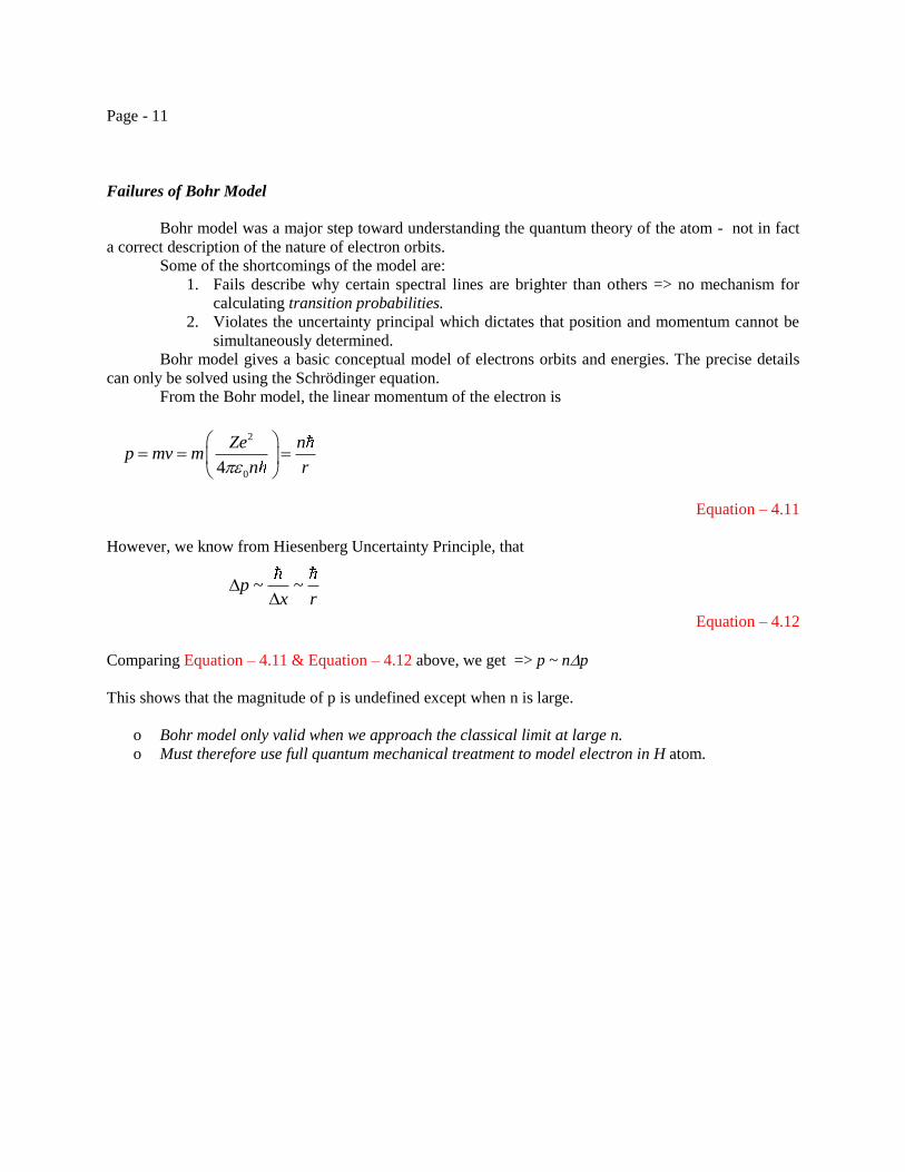
From the Bohr model, the linear momentum of the electron is

Equation – 4.11

However, we know from Hiesenberg Uncertainty Principle, that

Equation – 4.12

Comparing Equation – 4.11 & Equation – 4.12 above, we get => p ~ np

This shows that the magnitude of p is undefined except when n is large.

o Bohr model only valid when we approach the classical limit at large n.

o Must therefore use full quantum mechanical treatment to model electron in H atom.

2

04

Ze np mv m

n r

~ ~px r

Page-12

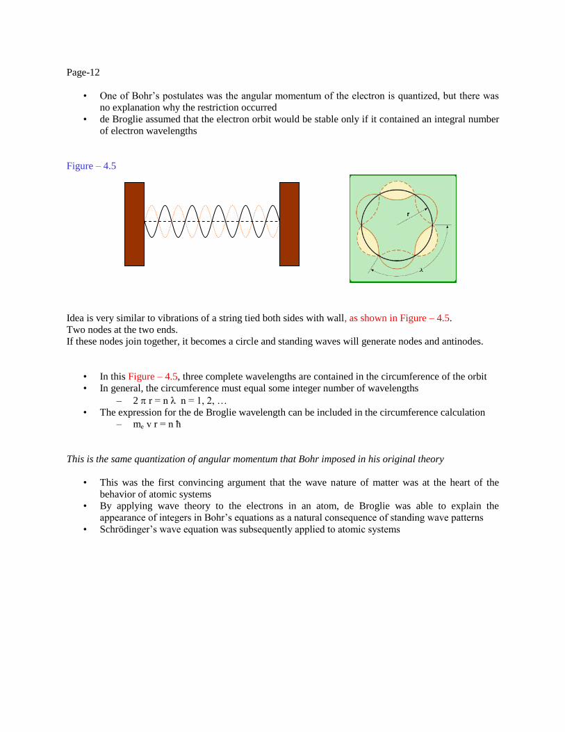
• One of Bohr’s postulates was the angular momentum of the electron is quantized, but there was

no explanation why the restriction occurred

• de Broglie assumed that the electron orbit would be stable only if it contained an integral number

of electron wavelengths

Figure – 4.5

Idea is very similar to vibrations of a string tied both sides with wall, as shown in Figure – 4.5.

Two nodes at the two ends.

If these nodes join together, it becomes a circle and standing waves will generate nodes and antinodes.

• In this Figure – 4.5, three complete wavelengths are contained in the circumference of the orbit

• In general, the circumference must equal some integer number of wavelengths

– 2 r = n λ n = 1, 2, …

• The expression for the de Broglie wavelength can be included in the circumference calculation

– me v r = n ħ

This is the same quantization of angular momentum that Bohr imposed in his original theory

• This was the first convincing argument that the wave nature of matter was at the heart of the

behavior of atomic systems

• By applying wave theory to the electrons in an atom, de Broglie was able to explain the

appearance of integers in Bohr’s equations as a natural consequence of standing wave patterns

• Schrödinger’s wave equation was subsequently applied to atomic systems

Page-13

Schrodinger Equation :

In 1926, Schrodinger said,

There is no reason to retain even Bohr’s electron orbits,

Basic equation governs wave motions and electron in a nuclear field.

If we consider, the electron as wave defined by de Broglie, we can treat the wave equation.

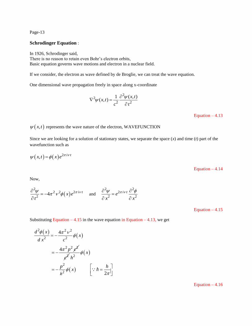
One dimensional wave propagation freely in space along x-coordinate

22

2 2

1 ( , )( , )

x tx t

c t

Equation – 4.13

,x t represents the wave nature of the electron, WAVEFUNCTION

Since we are looking for a solution of stationary states, we separate the space (x) and time (t) part of the

wavefunction such as

2, i tx t x e

Equation – 4.14

Now,

2

2 2 2

24 i tx e

t

and

2 22

2 2

i tex x

Equation – 4.15

Substituting Equation – 4.15 in the wave equation in Equation – 4.13, we get

2 2 2

2 2

2 2 2

4

4

d xx

d x c

p c

2c

2

2

2 2

xh

p hx

Equation – 4.16

Page-14

According to de Broglie wavelength,

&c c p c h

ph h

p

And the total energy (E) = kinetic energy + potential energy (V)

2

2

2

2

pV E

m

p m E V

Equation – 4.17

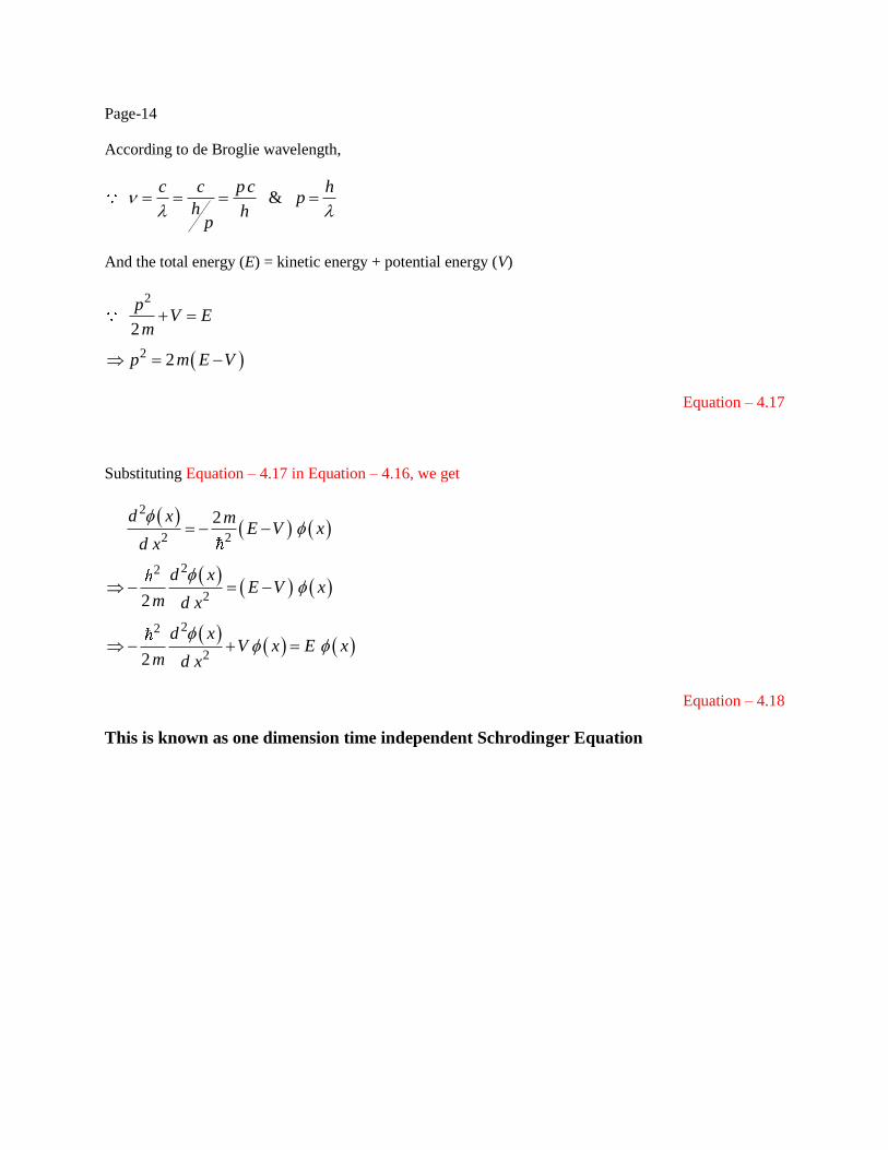
Substituting Equation – 4.17 in Equation – 4.16, we get

2

2 2

22

2

22

2

2

2

2

d x mE V x

d x

d xE V x

m d x

d xV x E x

m d x

Equation – 4.18

This is known as one dimension time independent Schrodinger Equation

Page-15

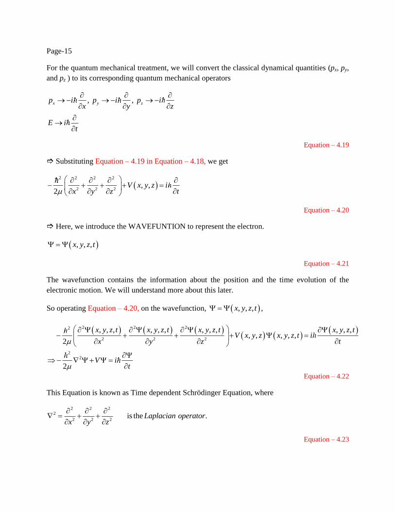
For the quantum mechanical treatment, we will convert the classical dynamical quantities (px, py,

and pz ) to its corresponding quantum mechanical operators

, ,x y zp i p i p ix y z

E it

Equation – 4.19

Substituting Equation – 4.19 in Equation – 4.18, we get

2 2 2 2

2 2 2, ,

2V x y z i

x y z t

Equation – 4.20

Here, we introduce the WAVEFUNTION to represent the electron.

, , ,x y z t

Equation – 4.21

The wavefunction contains the information about the position and the time evolution of the

electronic motion. We will understand more about this later.

So operating Equation – 4.20, on the wavefunction, , , ,x y z t ,

2 2 22

2 2 2

22

, , , , , , , , , , , ,, , , , ,

2

2

x y z t x y z t x y z t x y z tV x y z x y z t i

x y z t

V it

Equation – 4.22

This Equation is known as Time dependent Schrödinger Equation, where

2 2 2

2

2 2 2is the .Laplacian operator

x y z

Equation – 4.23

Page-16

The three dimensional Schrodinger Equation is

22

22

d rV r E r

m d x

Equation – 4.24

If we take the potential of the electron due to nucleus is

Equation – 4.25

Where r is the distance between the electron and the nucleus and Z is the charge (Z = 1 for hydrogen).

Substituting the potential in the Schrödinger Equation,

the energy becomes

Equation – 4.26

Where n is known as the principal quantum number.

Details of this quantum mechanical calculation are given

later.

This energy is exactly the same energy expression

derived by Bohr. In this figure, E (n=1) = -110000 cm-1

.

2ZeV

r

4 2

2 2

1

2n

me zE

n

Figure – 4.6

Page-17

Recap

In this lecture, we came to know about the development of quantization of matter and light.

We came to know the need for quantum mechanics for describing the light matter interaction in the

microscopic level.

We understood the microscopic region where the wave particle duality is valid.

We also came to know how Schrodinger developed his famous Schrodinger equation.