Quantitative Weather Impacts:

An Integrated Weather Effects Decision Aid Impact Magnitude Gradation Scheme and Friendly Versus Threat Delta Advantage

by Richard J. Szymber and Terry C. Jameson

ARL-TR-6539 August 2013 Approved for public release; distribution is unlimited.

NOTICES

Disclaimers The findings in this report are not to be construed as an official Department of the Army position unless so designated by other authorized documents. Citation of manufacturer’s or trade names does not constitute an official endorsement or approval of the use thereof. Destroy this report when it is no longer needed. Do not return it to the originator.

Army Research Laboratory White Sands Missile Range, NM 88002-5501

ARL-TR-6539 August 2013

Quantitative Weather Impacts: An Integrated Weather Effects Decision Aid Impact Magnitude Gradation Scheme and Friendly Versus Threat Delta Advantage

Richard J. Szymber and Terry C. Jameson

Computational and Information Sciences Directorate, ARL Approved for public release; distribution is unlimited.

ii

REPORT DOCUMENTATION PAGE Form Approved OMB No. 0704-0188

Public reporting burden for this collection of information is estimated to average 1 hour per response, including the time for reviewing instructions, searching existing data sources, gathering and maintaining the data needed, and completing and reviewing the collection information. Send comments regarding this burden estimate or any other aspect of this collection of information, including suggestions for reducing the burden, to Department of Defense, Washington Headquarters Services, Directorate for Information Operations and Reports (0704-0188), 1215 Jefferson Davis Highway, Suite 1204, Arlington, VA 22202-4302. Respondents should be aware that notwithstanding any other provision of law, no person shall be subject to any penalty for failing to comply with a collection of information if it does not display a currently valid OMB control number. PLEASE DO NOT RETURN YOUR FORM TO THE ABOVE ADDRESS. 1. REPORT DATE (DD-MM-YYYY)

August 2013 2. REPORT TYPE

Final 3. DATES COVERED (From - To)

01 January 2011–30 June 2013 4. TITLE AND SUBTITLE

Quantitative Weather Impacts: An Integrated Weather Effects Decision Aid Impact Magnitude Gradation Scheme and Friendly Versus Threat Delta Advantage

5a. CONTRACT NUMBER

5b. GRANT NUMBER

5c. PROGRAM ELEMENT NUMBER

6. AUTHOR(S)

Richard J. Szymber and Terry C. Jameson 5d. PROJECT NUMBER

5e. TASK NUMBER

5f. WORK UNIT NUMBER

7. PERFORMING ORGANIZATION NAME(S) AND ADDRESS(ES)

U.S. Army Research Laboratory Computational and Information Sciences Directorate Battlefield Environment Division (ATTN: RDRL-CIE-M) White Sands Missile Range, NM 88002-5501

8. PERFORMING ORGANIZATION REPORT NUMBER

ARL-TR-6539

9. SPONSORING/MONITORING AGENCY NAME(S) AND ADDRESS(ES)

10. SPONSOR/MONITOR’S ACRONYM(S) 11. SPONSOR/MONITOR'S REPORT NUMBER(S)

12. DISTRIBUTION/AVAILABILITY STATEMENT

Approved for public release; distribution is unlimited.

13. SUPPLEMENTARY NOTES

14. ABSTRACT

A fielded, rules-based weather effects decision support tool (DST) is limited in the detail of its display and the means by which it assesses the severity of the meteorological impacts. A prototype DST is described in this report that: (1) adds significant granularity to the weather impacts display; (2) accounts for the magnitude of the forecast weather parameters; and (3) allows for a quantitative comparison between friendly and enemy forces as to which side will be most impacted by adverse weather conditions.

15. SUBJECT TERMS

impact value, cell impact score, threshold value, parameter weighting

16. SECURITY CLASSIFICATION OF: 17. LIMITATION OF ABSTRACT

UU

18. NUMBER OF PAGES

60

19a. NAME OF RESPONSIBLE PERSON Terry C. Jameson

a. REPORT

Unclassified b. ABSTRACT

Unclassified c. THIS PAGE

Unclassified 19b. TELEPHONE NUMBER (Include area code) (575) 678-3924

Standard Form 298 (Rev. 8/98) Prescribed by ANSI Std. Z39.18

iii

Contents

List of Figures v

List of Tables vi

1. Summary 1

2. Introduction 1

3. Quantitative Weather Impacts—Background and Parameter Weighting Scheme 3

4. Impact Magnitude Gradation Scheme 5

4.1 Modified impact Value Computations ............................................................................5 4.1.1 Background .........................................................................................................5 4.1.2 Zero Percent and One-Hundred Percent Degradation Thresholds ......................6 4.1.3 Forecast Value—Modified Impact Value Linear Relationship ...........................9 4.1.4 A Negative Slope Example ...............................................................................10 4.1.5 IMGS_FVTDA Output of Thresholds and Line Segment Definitions .............12 4.1.6 Verification of Maximum and Minimum Thresholds .......................................14 4.1.7 Verification of Line Segment Slope/y-Intercept Values ...................................15 4.1.8 Forecast Values .................................................................................................16 4.1.9 Modified Impact Values From IMGS_FVTDA ................................................18 4.1.10 Verification of Modified Impact Values ...........................................................21

4.2 Cell Impact Score Computations ...................................................................................26 4.2.1 Basics of the CIS ...............................................................................................26 4.2.2 CIS Example Computation ................................................................................26 4.2.3 CIS Output Arrays .............................................................................................27

5. Friendly Versus Threat Delta Advantage 29

6. Discussion 35

7. Conclusions 36

8. References 39

iv

Appendix. IMGS/FVTDA Outline-Flowchart 41

List of Symbols, Abbreviations, and Acronyms 47

Distribution List 48

v

List of Figures

Figure 1. The current IWEDA “stoplight” color-code scheme, with corresponding percent of system degradation due to adverse weather, and the percent system effectiveness indicated on the left and right vertical axes, respectively (based on FM 34-81-1, 1992). .............................................................................................................................2

Figure 2. High-granularity PWS/CIS impact color code (right side). The CIS scale is indicated on the right-hand vertical axis and the corresponding percent mission degradation due to adverse weather is depicted on the left axis. By way of comparison, the legacy IWEDA “stoplight” scale is depicted on the left. ....................4

Figure 3. Comparison between a simulation of the legacy IWEDA IVs and the resulting CIS values. The PWS analysis included six parameters with varying parameter weights. A 100 × 100 km, Army Brigade-sized Area of Interest (AOI) is simulated (Szymber, 2006). ............................................................................................................5

Figure 4. The first phase of the IMGS process. The “green-amber” transition threshold (in this case, 20 kts) and the “amber-red” transition threshold (in this case, 40 kts) are known values. The thresholds at which 0% degradation and 100% degradation occur are unknowns and must be computed. A linear relationship is assumed across the 0% to 100% spectrum, hence the basis for conducting the extrapolations to these points. .7

Figure 5. The second phase of the IMGS process is shown during which the linear relationships between FV and MIV are established for the three line segments. In this case the slopes of the green and red segments are equal. ............................................10

Figure 6. The first phase of the IMGS process—is now for a parameter (Visibility) with a negatively sloping linear relationship between FV and percent degradation. .............11

Figure 7. The second phase of the IMGS process, for “Visibility.” In this case, the slopes of the green and red segments differ, since the extrapolated 100% degradation threshold had to be adjusted from a physically impossible value. ...............................12

Figure 8. IMGS color-coded impacts overlay of CIS output from table 19. .....................28

Figure 9. FVTDA definitions and criteria for degree of Friendly advantage and disadvantage (or Threat advantage) showing ∆CIS breakpoints and ranges with associated color coding. ...............................................................................................30

Figure 10. Graphical representation of the ∆CIS color-code scheme over the range of advantage/disadvantage categories as defined in figure 9. ..........................................31

Figure 11. Representation of the ∆CIS color-code scheme for the degree of Friendly advantage .....................................................................................................................31

Figure 12. Notional display of the FVTDA output over the AOI ......................................32

Figure 13. FVTDA color-coded advantage/disadvantage overlay of the ∆CIS output from table 23. ........................................................................................................................35

Figure 14. Meteorological critical value impact function notional example for surface wind speed ...................................................................................................................36

vi

List of Tables

Table 1. Equation development solving “min_G_TH” and “max_R_TH.” ........................8

Table 2. The IMGS_FVTDA output file named “thresh_slope_intcpt.txt” showing the computations of the “max_R_TH”, “min_G_TH” and the “slp” and “y-int” values for the three line segments for “wind speed” (WSP), “temperature” (TMP), and “cloud ceiling” (CIG). .............................................................................................................13

Table 3. The IMGS_FVTDA output file named “thresh_slope_intcpt.txt” showing the computations of the “max_R_TH”, “min_G_TH” and the “slp” and “y-int” values for the three line segments for “visibility” (VIS), “snow depth” (SNO), and “precipitation rate” (PCP). ..................................................................................................................14

Table 4. Excel vs. IMGS_FVTDA comparison of the “max_R_TH” and “min_G_TH” values for the six Met parameters. The slope and y-intercept values highlighted in yellow are for the linear extrapolation lines as depicted in the formulae in table 1 and not for the final FV-MIV line segments. The physically impossible thresholds for “VIS” and “PCP” are also highlighted.........................................................................15

Table 5. Comparisons of the “slp” and “y-int” values for the three line segments of the six Met parameters. ......................................................................................................16

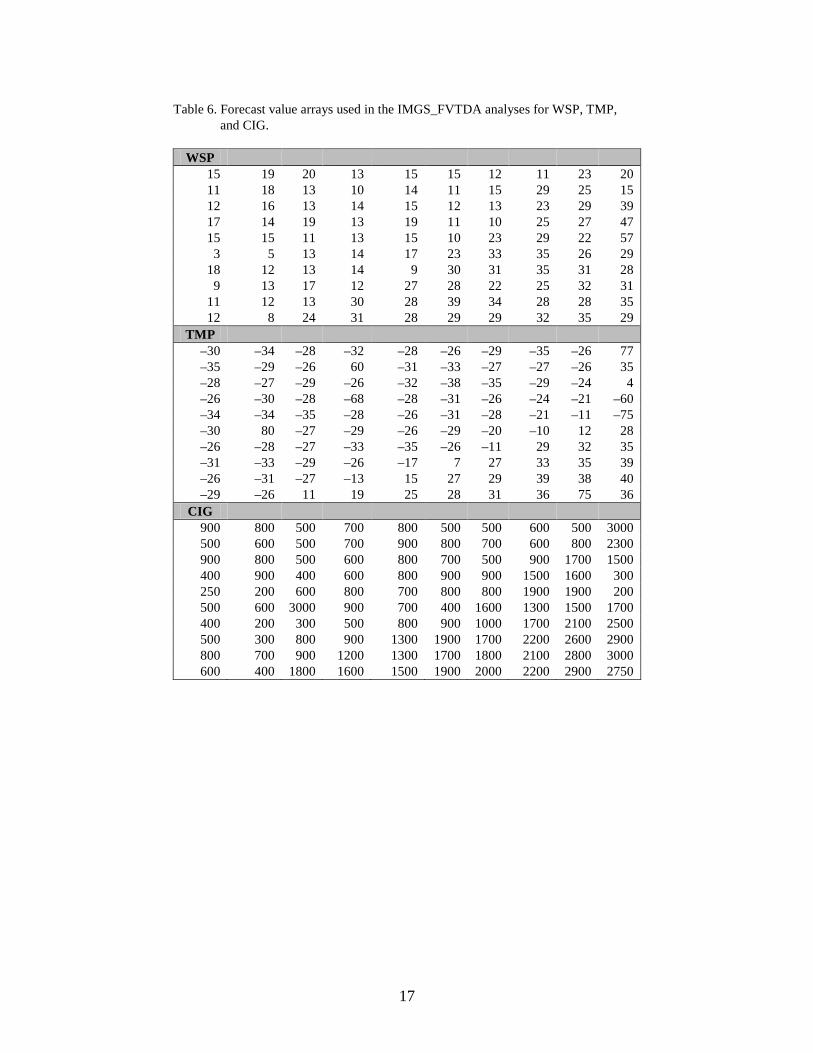
Table 6. Forecast value arrays used in the IMGS_FVTDA analyses for WSP, TMP, and CIG. ..............................................................................................................................17

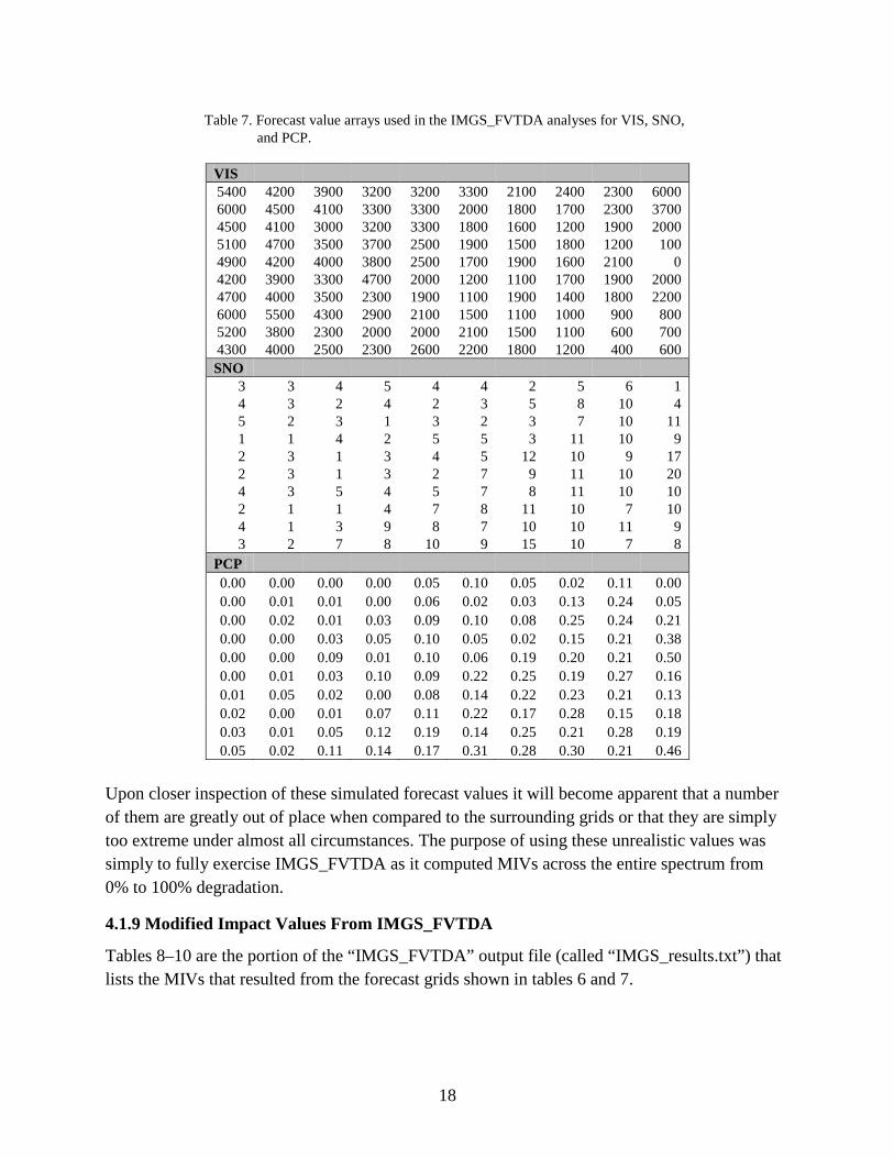
Table 7. Forecast value arrays used in the IMGS_FVTDA analyses for VIS, SNO, and PCP. .............................................................................................................................18

Table 8. Modified impact values for wind speed and surface temperature. ......................19

Table 9. Modified impact values for ceiling and visibility. ...............................................20

Table 10. Modified impact values for snow depth and precipitation rate. ........................21

Table 11. FV threshold names used for MIV checks.........................................................22

Table 12. MIV computations via Excel spreadsheet and IMGS_FVTDA for WSP. ........23

Table 13. MIV computations via Excel spreadsheet and IMGS_FVTDA for TMP. ........23

Table 14. MIV computations via Excel spreadsheet and IMGS_FVTDA for CIG. ..........24

Table 15. MIV computations via Excel SPREADSHEET and IMGS_FVTDA for VIS. .24

Table 16. MIV computations via Excel spreadsheet and IMGS_FVTDA for SNO. .........25

Table 17. MIV computations via Excel spreadsheet and IMGS_FVTDA for PCP. ..........25

Table 18. Generic CIS computation...................................................................................27

Table 19. CIS output array. ................................................................................................27

Table 20. Excel spreadsheet verification of CIS values. ...................................................29

Table 21. Friendly and threat CIS output based on the given weather and tactical scenario. .......................................................................................................................33

vii

Table 22. Friendly and threat CIS output based on the given weather and tactical scenario. .......................................................................................................................34

Table 23. FVTDA output of ∆CIS based on the given Friendly/Threat forces tactical, wintertime scenario. .....................................................................................................34

viii

INTENTIONALLY LEFT BLANK.

1

1. Summary

Currently, the rule impacts (favorable, marginal, or unfavorable) used by the Integrated Weather Effects Decision Aid (IWEDA) are shown on color-coded (green/yellow/red) weather effects matrices and map overlays. Transitions between these coarse-granularity, color-coded impacts are set up as step functions that do not portray a continuum of values, as would be expected in real-atmosphere transitions. Impacts rules are essentially equally-weighted and entirely system/sub-system/component-oriented, affording the commander no options to adjust for specific mission needs. No distinction is made in the impacts display for how many rules “fired,” with only the single, worst case “bubbling-up” to be displayed; nor is any adjustment made to account for how greatly the threshold values were exceeded. The goal of the Quantitative Weather Impacts project is to develop a series of interrelated methodologies, including Cell Impact Scores, a Parameter Weighting Scheme, and an Impact Magnitude Gradation Scheme, which will enable quantitative and highly granular weather impacts to be computed and displayed. Also, there is presently no quantitative means of assessing Friendly and Threat weather impacts concurrently using the IWEDA system. Manual comparisons between separate IWEDA runs are qualitative, time-consuming, difficult to visualize, and possibly inaccurate. Ultimately these new methodologies will enable an automated assessment of which force on the battlefield holds the advantage due to weather effects; this end-product has been termed the Friendly Versus Threat Delta Advantage.

2. Introduction

The IWEDA, originally developed by the U.S. Army Research Laboratory (ARL) in 1992, has been fielded on a military intelligence system called the Integrated Meteorological System (IMETS) since 1997 to provide tactical weather support to the U.S. Army. Background information describing the IWEDA software and its capabilities has been documented by Sauter et al. (1999) and verification/validation studies have been summarized by Raby et al. (2003). The Army IWEDA rules database (the Centralized Rules Data Base [CRDB]) and model software developed by ARL were officially certified and accredited for the Army by the U.S. Army and Intelligence Center and Fort Huachuca, AZ, in 2006 (Department of the Army, Memorandum, 2006). Underlying information on the IWEDA rules set development, description, assumptions, and criteria is contained in Szymber (2008).

Meteorological (MET) effects critical values are those values of weather factors (i.e., the critical thresholds) that, when exceeded, can significantly reduce the effectiveness of or prevent execution of tactical operations and/or the employment of weapon systems. Critical values define

2

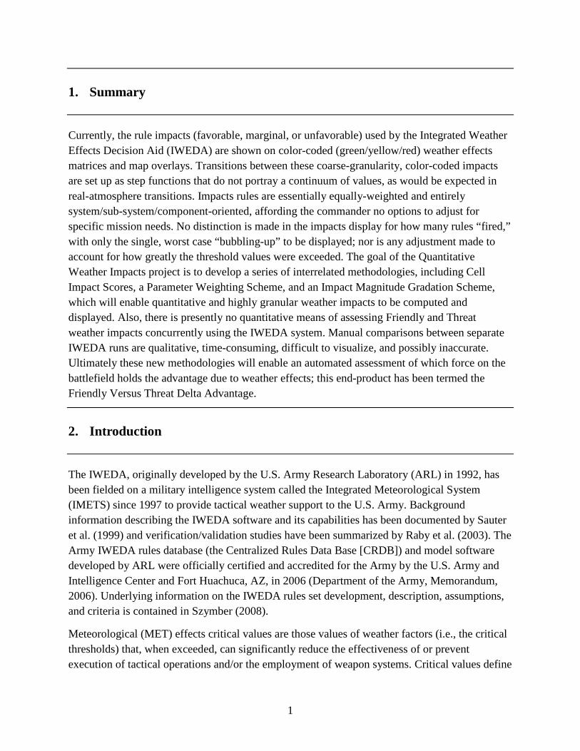
the operational limits beyond which it is not feasible to operate because of safety considerations or decreasing effectiveness. In fact, significant variations exceeding the critical value can prevent the successful accomplishment of an entire mission. These operational limits are usually based on tests conducted during weapon system development, the operational experience of weapon system users, expertise of subject matter experts, and/or military doctrine and regulations. The meteorological impacts are color coded in a “stoplight” format as follows (see figure 1):

• RED = Unfavorable: Severe or even total degradation/impact (>70% degradation). Exceeds operational limits or safety criteria

• AMBER = Marginal: Operational capability degraded. Moderate degradation/impact (30%–70% degradation)

• GREEN = Favorable: No operational restrictions. No or low degradation/impact (<30% degradation)

MET critical values are the lowest common denominator in assessing: (1) weather support requirements; (2) specific effects of weather on any system, subsystem, operation, tactic, and personnel; and (3) who has the tactical advantage in adverse weather—Friendly or Threat forces. They are the basis upon which weather effects and warnings/advisories are established, and are the bridge or connection between the battlespace weather and its warfighting operational impact. An accurate, complete database of critical threshold values and impacts for both Friendly and Threat capabilities is essential for effective Army weather support and operations.

Over the years of IWEDA use, observations have emerged identifying needs for its improvement including: (1) a need to derive overall mission impact due to adverse weather conditions, rather than simply presenting “worst-case” conditions for specific weapon systems; and (2) a need to better-represent the discrete color-coded Impact Values (IVs).

Figure 1. The current IWEDA “stoplight” color-code scheme, with corresponding percent of system degradation due to adverse weather, and the percent system effectiveness indicated on the left and right vertical axes, respectively (based on FM 34-81-1, 1992).

3

3. Quantitative Weather Impacts—Background and Parameter Weighting Scheme

There are several problems being addressed by the Quantitative Weather Impacts (QWI) development. The lack of a quantitative weather impacts system makes it impossible to discern or display the degree of impact and to assess advantages Friendly forces might have over the Threat due to prevailing MET conditions. A new weather effects display methodology is needed that will: (1) quantify the degree of weather impacts; (2) apply a color scheme with significantly more granularity in depicting the impacts; (3) accommodate varying weights of the individual weather parameters that are creating the impacts; (4) account for the degree to which weather thresholds are exceeded by forecast values in the analysis; and (5) allow a quantitative comparison between weather impacts on Friendly and Threat systems and missions.

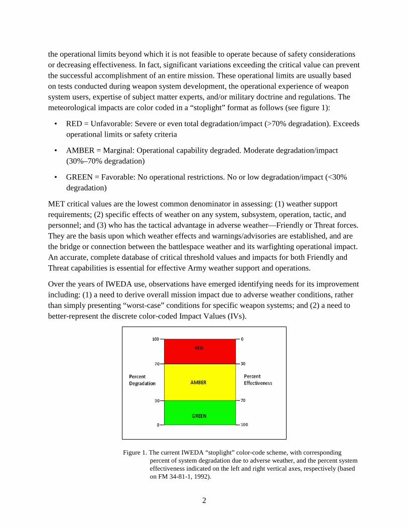
The QWI project, as it is currently known, has proceeded through several steps leading up to its present capabilities. QWI was conceived in order to add quantitative value and more granularity to the traditional IWEDA “stoplight” code of green, amber, and red cell colors indicating IVs of 0, 1, and 2, respectively. At its core, QWI was intended to answer the long-standing question in the weather impacts displays of “how red is red?”

The first phase of the QWI development was called the Parameter Weighting Scheme (PWS). Java code was written to prototype and test the PWS. Input to the PWS code is comprised of grids of IVs for a set of weather parameters coupled with a designation of how heavily each parameter is to be weighted. The PWS output consists of a grid of numerical Cell Impact Score (CIS) values along with a grid of corresponding cell color designations. The PWS is a highly granular, quantitative assessment of overall weather impacts applied to a mission-oriented “super set” of MET parameters (Szymber et al., 2011). Figure 2 depicts a comparison between the original IWEDA “stoplight” impact values and the CIS color scale.

4

Figure 2. High-granularity PWS/CIS impact color code (right side). The CIS scale is indicated on the right-hand vertical axis and the corresponding percent mission degradation due to adverse weather is depicted on the left axis. By way of comparison, the legacy IWEDA “stoplight” scale is depicted on the left.

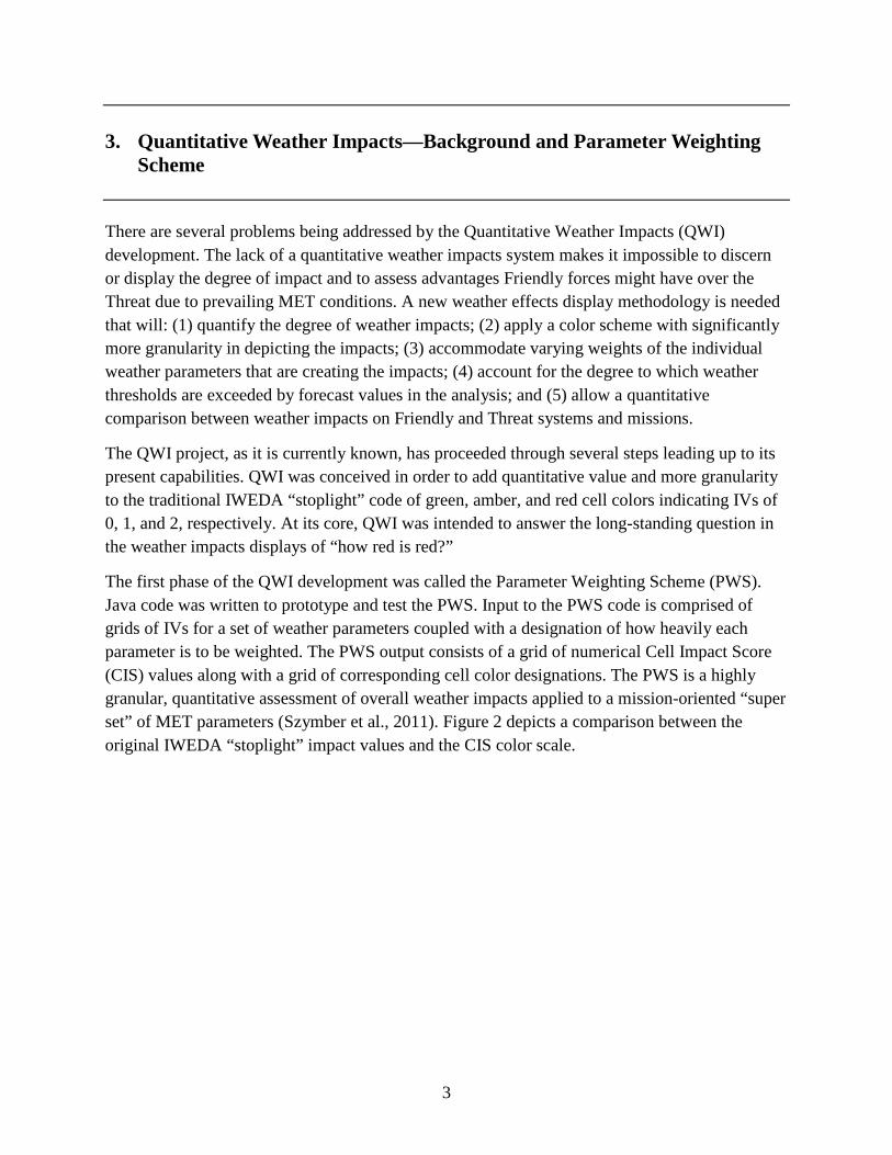
A comparison using simulated IVs, as might be produced from the legacy IWEDA and the PWS is shown in figure 3. The figure shows how the relative severity of the weather impacts in individual grid cells can be more accurately assessed using the PWS methodology.

5

Figure 3. Comparison between a simulation of the legacy IWEDA IVs and the resulting CIS values. The PWS analysis included six parameters with varying parameter weights. A 100 × 100 km, Army Brigade-sized Area of Interest (AOI) is simulated (Szymber, 2006).

Figure 3 shows how a significantly different weather impacts picture emerges when the number of thresholds being exceeded is taken into account and when varying MET parameter weights are applied.

4. Impact Magnitude Gradation Scheme

4.1 Modified impact Value Computations

4.1.1 Background

While the PWS does account for how many weather parameter rules are “firing” either “green,” “amber,” or “red,” within a given grid cell, there is no means to account for how much the forecast values are exceeding the rules thresholds. As an example, if a wind speed rule under the current IWEDA system has a “red” threshold of 40 kts, a forecast of 40 kts in a grid cell would result in an IV = 2 with the corresponding red cell color (as would a forecast of any greater speed). Clearly a wind speed of 60 kts would impose a much greater physical impact on an individual weapon system or an overall mission than one of 40 kts; and yet, it is not depicted in

6

the legacy IWEDA. In fact, because of the way the IVs are determined, the assumption within the IWEDA system is that a “red” cell color is indicative of a battlefield system performance degradation of anywhere between 70% and 100% with no means of determining the exact value. Since PWS is based upon the legacy IWEDA IVs, it is limited in the same way—and IMGS was designed to remove this limitation. This concept of accounting for the magnitude of a forecast value has been termed “threshold-exceeding.” The second phase of the QWI, called the Impact Magnitude Gradation Scheme (IMGS), was initiated to account for “threshold-exceeding.” Within the IMGS code a series of linear relationships are developed that relate a parameter’s forecast value (FV) to a modified impact value (MIV).* For example, under the IMGS system, a wind speed forecast of 40 kts would result in a MIV of 2.00—just at the “red” degradation threshold; whereas, a forecast of 50 kts might result in a MIV of 2.65. In all cases the maximum possible MIV has been set to 3.00 corresponding to 100% weather impacts degradation. The same basic code was used for IMGS as for the PWS (called “IMGS_FVTDA.java”), except that floating-point MIVs (a 0.00–3.00 scale) were input to the CIS calculations rather than the 0, 1, and 2 IV integers.

4.1.2 Zero Percent and One-Hundred Percent Degradation Thresholds

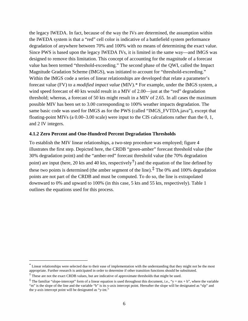
To establish the MIV linear relationships, a two-step procedure was employed; figure 4 illustrates the first step. Depicted here, the CRDB “green-amber” forecast threshold value (the 30% degradation point) and the “amber-red” forecast threshold value (the 70% degradation point) are input (here, 20 kts and 40 kts, respectively†) and the equation of the line defined by these two points is determined (the amber segment of the line).‡ The 0% and 100% degradation points are not part of the CRDB and must be computed. To do so, the line is extrapolated downward to 0% and upward to 100% (in this case, 5 kts and 55 kts, respectively). Table 1 outlines the equations used for this process.

* Linear relationships were selected due to their ease of implementation with the understanding that they might not be the most appropriate. Further research is anticipated in order to determine if other transition functions should be substituted. † These are not the exact CRDB values, but are indicative of approximate thresholds that might be used. ‡ The familiar “slope-intercept” form of a linear equation is used throughout this document, i.e., “y = mx + b”, where the variable “m” is the slope of the line and the variable “b” is its y-axis intercept point. Hereafter the slope will be designated as “slp” and the y-axis intercept point will be designated as “y-int.”

7

Figure 4. The first phase of the IMGS process. The “green-amber” transition threshold (in this case, 20 kts) and the “amber-red” transition threshold (in this case, 40 kts) are known values. The thresholds at which 0% degradation and 100% degradation occur are unknowns and must be computed. A linear relationship is assumed across the 0% to 100% spectrum, hence the basis for conducting the extrapolations to these points.

8

Table 1. Equation development solving “min_G_TH” and “max_R_TH.”

Legend: “A_R_TH” …The amber-red threshold forecast value (“TH” refers to a generic threshold value)

“G_A_TH” …The green-amber threshold forecast value

“slp” … The slope of the line

“y-int” … The y-intercept of the line

“pct-deg” … Percent degradation

“min_G_TH”… The threshold at which 0% degradation in the “green” region is encountered

“max_R_TH” … The threshold at which 100% degradation in the “red” region is encountered

pct-deg = slp * TH + y-int (This is the basic slope/intercept equation for the “FV-pct-deg” line)

Solving for the slope:a

slp = 40/(A_R_TH – G_A_TH) (1)

Note: “40” (40%) is the delta-Y value (the delta “pct-deg”) between the two known thresholds. Within the IWEDA system it is always the same value, i.e. 40%. With the slope computed, solving for the y-intercept:

y-int = pct-deg – slp * TH (2)

y-int = 70 – slp * A_R_TH (3)

Note: “70” is the percent degradation at the ‘A_R_TH’ threshold. The same “y-int” results from inputting “30” (for 30% degradation, and “G_A_TH” for the threshold).

With the slope and y-intercept known, inserting “0” for the 0% percent degradation:

0 = slp * min_G_TH + y-int (4)

Solving for the forecast threshold at which 0% degradation occurs:

min_G_TH = -(y-int)/slp (5)

Inserting “100” for the percent degradation:

100 = slp * max_R_TH + y-int (6)

Solving for the forecast threshold at which 100% degradation occurs.

max_R_TH = (100 - y-int)/slp (7)

a Equations 1, 3, 5, and 7 (in bold) were used in the IMGS_FVTDA Java code. Equations 2, 4, and 6 indicate interim steps.

9

4.1.3 Forecast Value—Modified Impact Value Linear Relationship

With the set of four threshold values known, the second step in the MIV development process can proceed. In this step, linear relationships are established between the forecast value and the MIV itself. Variations of equations 1 and 2 from table 1 were used to compute the line segment slopes and y-intercepts, respectively. Although in most cases the same slope results for both the “green” and “red” line segments (since these segments span the same amount of percent degradation, i.e., 30%)—a distinction is made between the two. This is done for several reasons:

1. While the slope is usually the same, the y-intercept value is not—thus the equations for these two line segments are never identical.

2. It made sense initially to set the maximum MIV equal to 3.00, so that the “red” line segment spans a range of MIVs of 1.00; as do the “green” and “amber” segments. The maximum MIV of 3.00 is not a hard-wired constant; however, it is a variable value that is assigned in one of IMGS_FVTDA’s input files. Although unlikely, it is possible that subsequent research will suggest that a value other than 3.00 would be more appropriate for the maximum MIV, and the input file would need to be adjusted accordingly. If this were to occur, the slope of the “red” line would immediately differ from that of the “green” line.

3. In testing the prototype IMGS_FVTDA it was noted that occasionally the extrapolation process depicted in figure 4 will produce a value for “min_G_TH” or “max_R_TH” that is a physical impossibility (for example, a negative value of a rainfall rate, visibility, or cloud ceiling height). In these cases, the “min_G_TH” or “max_R_TH” is reset by IMGS_FVTDA to be exactly equal to zero, thus altering the slope of the line segment slightly.

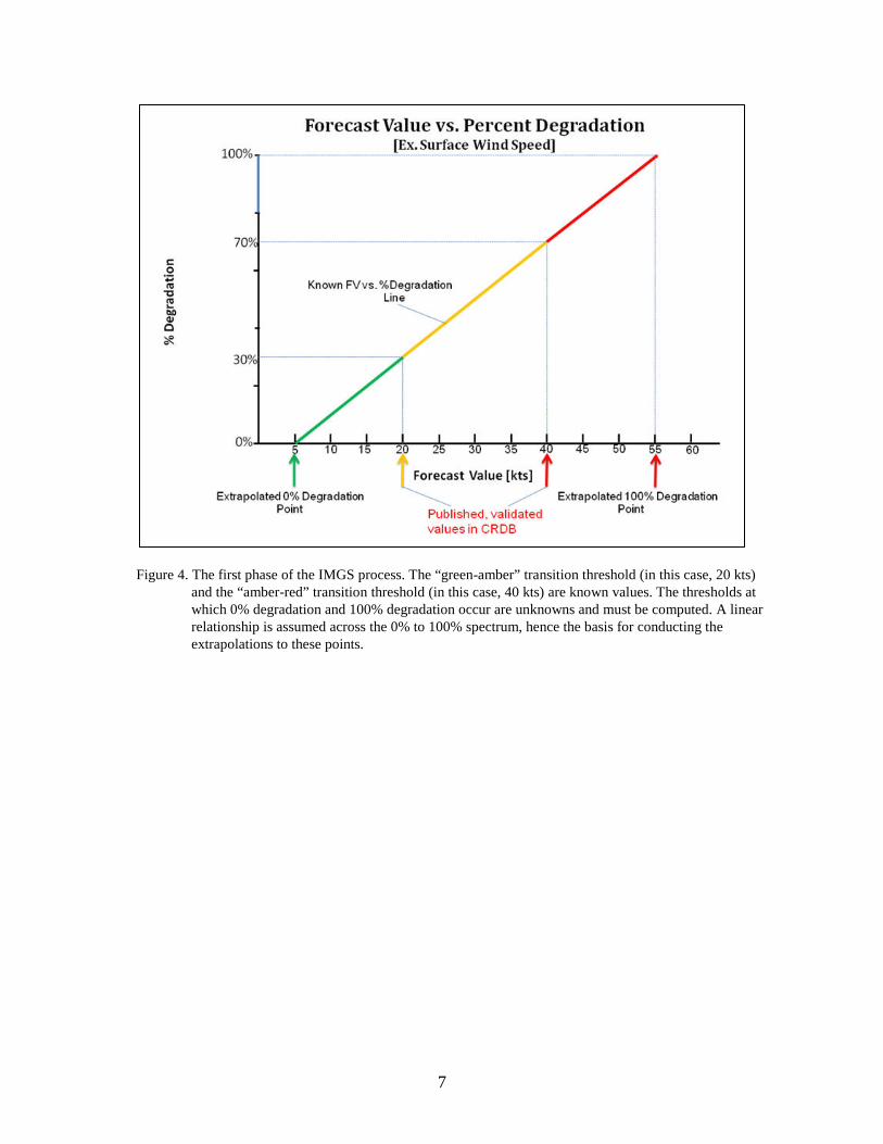
Figure 5 graphically depicts the process of establishing the slope-intercept equations for the three segments of the FV-MIV relationships for surface wind speed. As an example, the variable “R_MIVfv” stands for “the red line segment Modified Impact Value as a function of Forecast Value” and so forth for the “amber” and “green” segments. A number of points in regard to figure 5 should be noted. The “delta-Y” for each line segment is the same—a delta MIV of 1.0 (i.e., the “green” segment spans from 0.00 to 1.00, the “amber” from 1.00 to 2.00, and the “red” from 2.00 to 3.00). In this surface wind speed case, the slopes of the “green” and “red” line segments are identical (0.0667). This is because the “delta-X” for each line segment is the same as well (15 kts). The green line extending along the x-axis from 5 kts down to 0 kts simply indicates that a MIV of 0.00 is produced by IMGS_FVTDA for FVs in this range. Clearly, the linear FV-MIV equation will produce a negative MIV for FVs under 5 kts. IMGS_FVTDA automatically assigns a MIV = 0.00 when a negative value is computed. On the y-axis the maximum value of 3.00 is shown in red, which simply indicates that it is considered to be a variable value that could be adjusted somewhat if indicated by subsequent research. A red arrow extends horizontally to the right for FVs exceeding 55 kts. This indicates that, even though in this section MIVs greater than 3.00 will be computed using the “red” segment linear relationship,

10

IMGS_FVTDA automatically resets the MIV to be equal to 3.00. The two-color arrows at 20 kts and 40 kts indicate the FV threshold transitions. The arrows at 13 kts, 30 kts, and 47 kts show the resulting MIVs in the “green,” “amber,” and “red” segments, respectively (MIV = 0.53, 1.50, and 2.47, respectively). As indicated by the label, wind speed is an example of a MET parameter for which increasing FVs relate to increasing MIVs; consequently, the slopes of the lines are positive numbers. In the following example (visibility), the opposite will be the case.

Figure 5. The second phase of the IMGS process is shown during which the linear relationships between FV and MIV are established for the three line segments. In this case the slopes of the green and red segments are equal.

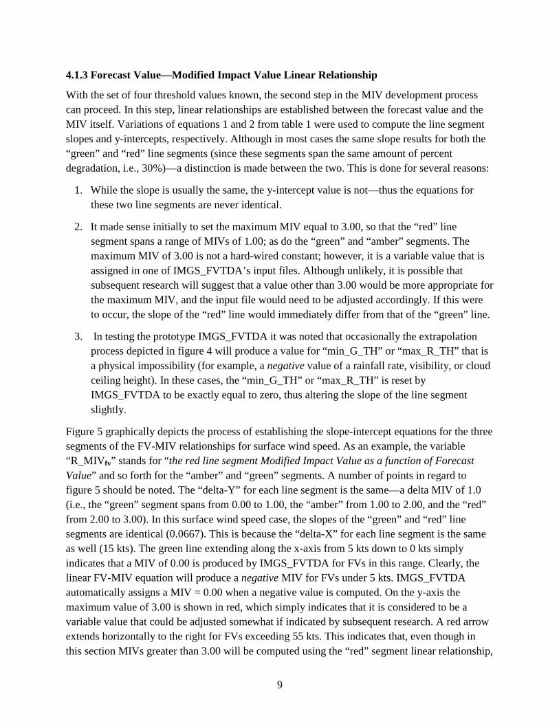
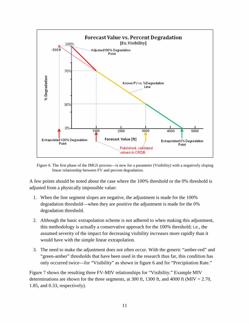
4.1.4 A Negative Slope Example

Figure 6 shows the extrapolation process for “Visibility” a parameter for which the severity of its impact decreases with increasing value. The linear extrapolation to the 0% degradation point yields a value of 4500 ft. The linear extrapolation to the 100% degradation point yields a physically impossible value of –500 ft in which case IMGS_FVTDA simply resets the value to 0 ft.

11

Figure 6. The first phase of the IMGS process—is now for a parameter (Visibility) with a negatively sloping linear relationship between FV and percent degradation.

A few points should be noted about the case where the 100% threshold or the 0% threshold is adjusted from a physically impossible value:

1. When the line segment slopes are negative, the adjustment is made for the 100% degradation threshold—when they are positive the adjustment is made for the 0% degradation threshold.

2. Although the basic extrapolation scheme is not adhered to when making this adjustment, this methodology is actually a conservative approach for the 100% threshold; i.e., the assumed severity of the impact for decreasing visibility increases more rapidly than it would have with the simple linear extrapolation.

3. The need to make the adjustment does not often occur. With the generic “amber-red” and “green-amber” thresholds that have been used in the research thus far, this condition has only occurred twice—for “Visibility” as shown in figure 6 and for “Precipitation Rate.”

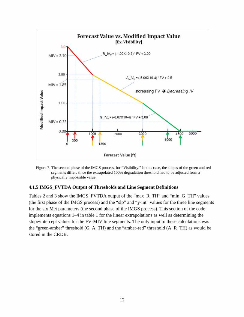
Figure 7 shows the resulting three FV-MIV relationships for “Visibility.” Example MIV determinations are shown for the three segments, at 300 ft, 1300 ft, and 4000 ft (MIV = 2.70, 1.85, and 0.33, respectively).

12

Figure 7. The second phase of the IMGS process, for “Visibility.” In this case, the slopes of the green and red segments differ, since the extrapolated 100% degradation threshold had to be adjusted from a physically impossible value.

4.1.5 IMGS_FVTDA Output of Thresholds and Line Segment Definitions

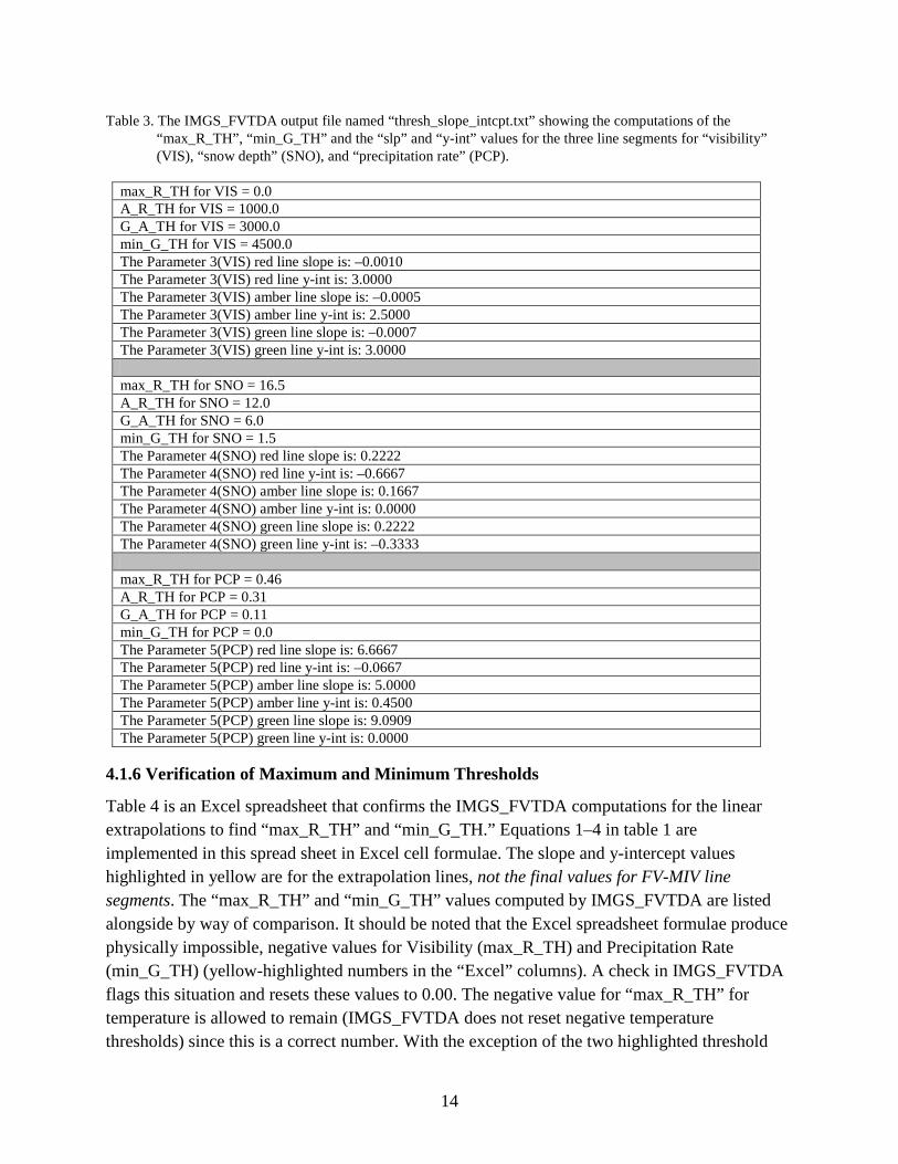
Tables 2 and 3 show the IMGS_FVTDA output of the “max_R_TH” and “min_G_TH” values (the first phase of the IMGS process) and the “slp” and “y-int” values for the three line segments for the six Met parameters (the second phase of the IMGS process). This section of the code implements equations 1–4 in table 1 for the linear extrapolations as well as determining the slope/intercept values for the FV-MIV line segments. The only input to these calculations was the “green-amber” threshold (G_A_TH) and the “amber-red” threshold (A_R_TH) as would be stored in the CRDB.

13

Table 2. The IMGS_FVTDA output file named “thresh_slope_intcpt.txt” showing the computations of the “max_R_TH”, “min_G_TH” and the “slp” and “y-int” values for the three line segments for “wind speed” (WSP), “temperature” (TMP), and “cloud ceiling” (CIG).

max_R_TH for WSP = 55.0 A_R_TH for WSP = 40.0 G_A_TH for WSP = 20.0 min_G_TH for WSP = 5.0 The Parameter 0(WSP) red line slope is: 0.0667 The Parameter 0(WSP) red line y-int is: –0.6667 The Parameter 0(WSP) amber line slope is: 0.0500 The Parameter 0(WSP) amber line y-int is: 0.0000 The Parameter 0(WSP) green line slope is: 0.0667 The Parameter 0(WSP) green line y-int is: –0.3333 max_R_TH for TMP = –67.75 A_R_TH for TMP = –25.0 G_A_TH for TMP = 32.0 min_G_TH for TMP = 74.75 The Parameter 1(TMP) red line slope is: –0.0234 The Parameter 1(TMP) red line y-int is: 1.4152 The Parameter 1(TMP) amber line slope is: –0.0175 The Parameter 1(TMP) amber line y-int is: 1.5614 The Parameter 1(TMP) green line slope is: –0.0234 The Parameter 1(TMP) green line y-int is: 1.7485 max_R_TH for CIG = 250.0 A_R_TH for CIG = 1000.0 G_A_TH for CIG = 2000.0 min_G_TH for CIG = 2750.0 The Parameter 2(CIG) red line slope is: –0.0013 The Parameter 2(CIG) red line y-int is: 3.3333 The Parameter 2(CIG) amber line slope is: –0.0010 The Parameter 2(CIG) amber line y-int is: 3.0000 The Parameter 2(CIG) green line slope is: –0.0013 The Parameter 2(CIG) green line y-int is: 3.6667

14

Table 3. The IMGS_FVTDA output file named “thresh_slope_intcpt.txt” showing the computations of the “max_R_TH”, “min_G_TH” and the “slp” and “y-int” values for the three line segments for “visibility” (VIS), “snow depth” (SNO), and “precipitation rate” (PCP).

max_R_TH for VIS = 0.0 A_R_TH for VIS = 1000.0 G_A_TH for VIS = 3000.0 min_G_TH for VIS = 4500.0 The Parameter 3(VIS) red line slope is: –0.0010 The Parameter 3(VIS) red line y-int is: 3.0000 The Parameter 3(VIS) amber line slope is: –0.0005 The Parameter 3(VIS) amber line y-int is: 2.5000 The Parameter 3(VIS) green line slope is: –0.0007 The Parameter 3(VIS) green line y-int is: 3.0000 max_R_TH for SNO = 16.5 A_R_TH for SNO = 12.0 G_A_TH for SNO = 6.0 min_G_TH for SNO = 1.5 The Parameter 4(SNO) red line slope is: 0.2222 The Parameter 4(SNO) red line y-int is: –0.6667 The Parameter 4(SNO) amber line slope is: 0.1667 The Parameter 4(SNO) amber line y-int is: 0.0000 The Parameter 4(SNO) green line slope is: 0.2222 The Parameter 4(SNO) green line y-int is: –0.3333 max_R_TH for PCP = 0.46 A_R_TH for PCP = 0.31 G_A_TH for PCP = 0.11 min_G_TH for PCP = 0.0 The Parameter 5(PCP) red line slope is: 6.6667 The Parameter 5(PCP) red line y-int is: –0.0667 The Parameter 5(PCP) amber line slope is: 5.0000 The Parameter 5(PCP) amber line y-int is: 0.4500 The Parameter 5(PCP) green line slope is: 9.0909 The Parameter 5(PCP) green line y-int is: 0.0000

4.1.6 Verification of Maximum and Minimum Thresholds

Table 4 is an Excel spreadsheet that confirms the IMGS_FVTDA computations for the linear extrapolations to find “max_R_TH” and “min_G_TH.” Equations 1–4 in table 1 are implemented in this spread sheet in Excel cell formulae. The slope and y-intercept values highlighted in yellow are for the extrapolation lines, not the final values for FV-MIV line segments. The “max_R_TH” and “min_G_TH” values computed by IMGS_FVTDA are listed alongside by way of comparison. It should be noted that the Excel spreadsheet formulae produce physically impossible, negative values for Visibility (max_R_TH) and Precipitation Rate (min_G_TH) (yellow-highlighted numbers in the “Excel” columns). A check in IMGS_FVTDA flags this situation and resets these values to 0.00. The negative value for “max_R_TH” for temperature is allowed to remain (IMGS_FVTDA does not reset negative temperature thresholds) since this is a correct number. With the exception of the two highlighted threshold

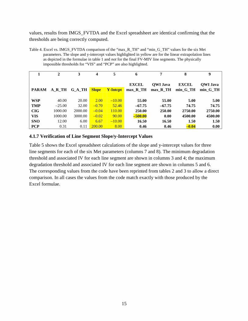
15

values, results from IMGS_FVTDA and the Excel spreadsheet are identical confirming that the thresholds are being correctly computed.

Table 4. Excel vs. IMGS_FVTDA comparison of the “max_R_TH” and “min_G_TH” values for the six Met parameters. The slope and y-intercept values highlighted in yellow are for the linear extrapolation lines as depicted in the formulae in table 1 and not for the final FV-MIV line segments. The physically impossible thresholds for “VIS” and “PCP” are also highlighted.

1 2 3 4 5 6 7 8 9

EXCEL QWI Java EXCEL QWI Java

PARAM A_R_TH G_A_TH Slope Y-Intcpt max_R_TH max_R_TH min_G_TH min_G_TH

WSP 40.00 20.00 2.00 –10.00 55.00 55.00 5.00 5.00 TMP –25.00 32.00 –0.70 52.46 –67.75 –67.75 74.75 74.75 CIG 1000.00 2000.00 –0.04 110.00 250.00 250.00 2750.00 2750.00 VIS 1000.00 3000.00 –0.02 90.00 –500.00 0.00 4500.00 4500.00 SNO 12.00 6.00 6.67 –10.00 16.50 16.50 1.50 1.50 PCP 0.31 0.11 200.00 8.00 0.46 0.46 –0.04 0.00

4.1.7 Verification of Line Segment Slope/y-Intercept Values

Table 5 shows the Excel spreadsheet calculations of the slope and y-intercept values for three line segments for each of the six Met parameters (columns 7 and 8). The minimum degradation threshold and associated IV for each line segment are shown in columns 3 and 4; the maximum degradation threshold and associated IV for each line segment are shown in columns 5 and 6. The corresponding values from the code have been reprinted from tables 2 and 3 to allow a direct comparison. In all cases the values from the code match exactly with those produced by the Excel formulae.

16

Table 5. Comparisons of the “slp” and “y-int” values for the three line segments of the six Met parameters.

1 2 3 4 5 6 7 8 9 10

MIN MIN MAX MAX

Degr.a Degr. Degr. Degr. EXCEL EXCEL QWI Java

QWI Java

Thresh. IV Thresh. IV Slope Y-Intcpt Slope Y-Intcpt

WSP RED 40 2 55 3 0.0667 –0.6667 0.0667 –0.6667

AMB 20 1 40 2 0.0500 0.0000 0.0500 0.0000

GRN 5 0 20 1 0.0667 –0.3333 0.0667 –0.3333

TMP RED –25 2 –67.75 3 –0.0234 1.4152 –0.0234 1.4152

AMB 32 1 –25 2 –0.0175 1.5614 –0.0175 1.5614

GRN 74.75 0 32 1 –0.0234 1.7485 –0.0234 1.7485

CIG RED 1000 2 250 3 –0.0013 3.3333 –0.0013 3.3333

AMB 2000 1 1000 2 –0.0010 3.0000 –0.0010 3.0000

GRN 2750 0 2000 1 –0.0013 3.6667 –0.0013 3.6667

VIS RED 1000 2 0 3 –0.0010 3.0000 –0.0010 3.0000

AMB 3000 1 1000 2 –0.0005 2.5000 –0.0005 2.5000

GRN 4500 0 3000 1 –0.0007 3.0000 –0.0007 3.0000

SNO RED 12 2 16.5 3 0.2222 –0.6667 0.2222 –0.6667

AMB 6 1 12 2 0.1667 0.0000 0.1667 0.0000

GRN 1.5 0 6 1 0.2222 –0.3333 0.2222 –0.3333

PCP RED 0.31 2 0.46 3 6.6667 –0.0667 6.6667 –0.0667

AMB 0.11 1 0.31 2 5.0000 0.4500 5.0000 0.4500

GRN 0 0 0.11 1 9.0909 0.0000 9.0909 0.0000 a Degradation

4.1.8 Forecast Values

Tables 6 and 7 show the simulated forecast values (for the six variables WSP, TMP, CIG, VIS, SNO, and PCP) that were input to IMGS_FVTDA for all CIS and FVTDA computations. In other words, these are not forecast values from the IWEDA Gridded Met Data Base. Instead, they were devised by the coauthors and intended to represent (for the most part) a wintertime scenario. Each cell value in these arrays is meant to emulate a grid forecast produced by a Numerical Weather Prediction (NWP) model at a single model level. (IMGS_FVTDA is able to produce CIS values for multiple NWP model levels; however, for the sake of brevity only the results from a single level will be investigated in this report).

17

Table 6. Forecast value arrays used in the IMGS_FVTDA analyses for WSP, TMP, and CIG.

WSP 15 19 20 13 15 15 12 11 23 20 11 18 13 10 14 11 15 29 25 15 12 16 13 14 15 12 13 23 29 39 17 14 19 13 19 11 10 25 27 47 15 15 11 13 15 10 23 29 22 57 3 5 13 14 17 23 33 35 26 29

18 12 13 14 9 30 31 35 31 28 9 13 17 12 27 28 22 25 32 31

11 12 13 30 28 39 34 28 28 35 12 8 24 31 28 29 29 32 35 29

TMP –30 –34 –28 –32 –28 –26 –29 –35 –26 77 –35 –29 –26 60 –31 –33 –27 –27 –26 35 –28 –27 –29 –26 –32 –38 –35 –29 –24 4 –26 –30 –28 –68 –28 –31 –26 –24 –21 –60 –34 –34 –35 –28 –26 –31 –28 –21 –11 –75 –30 80 –27 –29 –26 –29 –20 –10 12 28 –26 –28 –27 –33 –35 –26 –11 29 32 35 –31 –33 –29 –26 –17 7 27 33 35 39 –26 –31 –27 –13 15 27 29 39 38 40 –29 –26 11 19 25 28 31 36 75 36

CIG 900 800 500 700 800 500 500 600 500 3000 500 600 500 700 900 800 700 600 800 2300 900 800 500 600 800 700 500 900 1700 1500 400 900 400 600 800 900 900 1500 1600 300 250 200 600 800 700 800 800 1900 1900 200 500 600 3000 900 700 400 1600 1300 1500 1700 400 200 300 500 800 900 1000 1700 2100 2500 500 300 800 900 1300 1900 1700 2200 2600 2900 800 700 900 1200 1300 1700 1800 2100 2800 3000 600 400 1800 1600 1500 1900 2000 2200 2900 2750

18

Table 7. Forecast value arrays used in the IMGS_FVTDA analyses for VIS, SNO, and PCP.

VIS 5400 4200 3900 3200 3200 3300 2100 2400 2300 6000

6000 4500 4100 3300 3300 2000 1800 1700 2300 3700 4500 4100 3000 3200 3300 1800 1600 1200 1900 2000 5100 4700 3500 3700 2500 1900 1500 1800 1200 100 4900 4200 4000 3800 2500 1700 1900 1600 2100 0 4200 3900 3300 4700 2000 1200 1100 1700 1900 2000 4700 4000 3500 2300 1900 1100 1900 1400 1800 2200 6000 5500 4300 2900 2100 1500 1100 1000 900 800 5200 3800 2300 2000 2000 2100 1500 1100 600 700 4300 4000 2500 2300 2600 2200 1800 1200 400 600 SNO

3 3 4 5 4 4 2 5 6 1 4 3 2 4 2 3 5 8 10 4 5 2 3 1 3 2 3 7 10 11 1 1 4 2 5 5 3 11 10 9 2 3 1 3 4 5 12 10 9 17 2 3 1 3 2 7 9 11 10 20 4 3 5 4 5 7 8 11 10 10 2 1 1 4 7 8 11 10 7 10 4 1 3 9 8 7 10 10 11 9 3 2 7 8 10 9 15 10 7 8

PCP 0.00 0.00 0.00 0.00 0.05 0.10 0.05 0.02 0.11 0.00

0.00 0.01 0.01 0.00 0.06 0.02 0.03 0.13 0.24 0.05 0.00 0.02 0.01 0.03 0.09 0.10 0.08 0.25 0.24 0.21 0.00 0.00 0.03 0.05 0.10 0.05 0.02 0.15 0.21 0.38 0.00 0.00 0.09 0.01 0.10 0.06 0.19 0.20 0.21 0.50 0.00 0.01 0.03 0.10 0.09 0.22 0.25 0.19 0.27 0.16 0.01 0.05 0.02 0.00 0.08 0.14 0.22 0.23 0.21 0.13 0.02 0.00 0.01 0.07 0.11 0.22 0.17 0.28 0.15 0.18 0.03 0.01 0.05 0.12 0.19 0.14 0.25 0.21 0.28 0.19 0.05 0.02 0.11 0.14 0.17 0.31 0.28 0.30 0.21 0.46

Upon closer inspection of these simulated forecast values it will become apparent that a number of them are greatly out of place when compared to the surrounding grids or that they are simply too extreme under almost all circumstances. The purpose of using these unrealistic values was simply to fully exercise IMGS_FVTDA as it computed MIVs across the entire spectrum from 0% to 100% degradation.

4.1.9 Modified Impact Values From IMGS_FVTDA

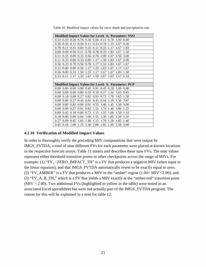
Tables 8–10 are the portion of the “IMGS_FVTDA” output file (called “IMGS_results.txt”) that lists the MIVs that resulted from the forecast grids shown in tables 6 and 7.

19

Table 8. Modified impact values for wind speed and surface temperature.

Modified Impact Values for Level: 0a, Parameter: WSP 0.67 0.93 1.00 0.53 0.67 0.67 0.47 0.40 1.15 1.00 0.40 0.87 0.53 0.33 0.60 0.40 0.67 1.45 1.25 0.67 0.47 0.73 0.53 0.60 0.67 0.47 0.53 1.15 1.45 2.07 0.80 0.60 0.93 0.53 0.93 0.40 0.33 1.25 1.35 3.00 0.67 0.67 0.40 0.53 0.67 0.33 1.15 1.45 1.10 3.00 0.00 0.00 0.53 0.60 0.80 1.15 1.65 1.75 1.30 1.45 0.87 0.47 0.53 0.60 0.27 1.50 1.55 1.75 1.55 1.40 0.27 0.53 0.80 0.47 1.35 1.40 1.10 1.25 1.60 1.55 0.40 0.47 0.53 1.50 1.40 2.00 1.70 1.40 1.40 1.75 0.47 0.20 1.20 1.55 1.40 1.45 1.45 1.60 1.75 1.45 Modified Impact Values for Level: 0, Parameter: TMP 2.12 2.21 2.07 2.16 2.07 2.02 2.09 2.23 2.02 0.00 2.23 2.09 2.02 0.35 2.14 2.19 2.05 2 .05 2.02 0.93 2.07 2.05 2.09 2.02 2.16 2.30 2.23 2.09 1.98 1.49 2.02 2.12 2.07 3.00 2.07 2.14 2.02 1.98 1.93 2.82 2.21 2.21 2.23 2.07 2.00 2.14 2.07 1.93 1.75 3.00 2.12 0.00 2.05 2.09 2.02 2.09 1.91 1.74 1.35 1.07 2.02 2.07 2.05 2.19 2.23 2.00 1.75 1.05 1.00 0.93 2.14 2.19 2.09 2.02 1.86 1.44 1.09 0.98 0.93 0.84 2.02 2.14 2.05 1.79 1.30 1.09 1.05 0.84 0.86 0.81 2.09 2.02 1.37 1.23 1.12 1.07 1.02 0.91 0.00 0.91

a “Level 0” refers to the lowest level in the simulated NWP model output grid.

20

Table 9. Modified impact values for ceiling and visibility.

Modified Impact Values for Level: 0, Parameter: CIG 2.13 2.27 2.67 2.40 2.27 2.67 2.67 2.53 2.67 0.00 2.67 2.53 2.67 2.40 2.13 2.27 2.40 2.53 2.27 0.60 2.13 2.27 2.67 2.53 2.27 2.40 2.67 2.13 1.30 1.50 2.80 2.13 2.80 2.53 2.27 2.13 2.13 1.50 1.40 2.93 3.00 3.00 2.53 2.27 2.40 2.27 2.27 1.10 1.10 3.00 2.67 2.53 0.00 2.13 2.40 2.80 1.40 1.70 1.50 1.30 2.80 3.00 2.93 2.67 2.27 2.13 2.00 1.30 0.87 0.33 2.67 2.93 2.27 2.13 1.70 1.10 1.30 0.73 0.20 0.00 2.27 2.40 2.13 1.80 1.70 1.30 1.20 0.87 0.00 0.00 2.53 2.80 1.20 1.40 1.50 1.10 1.00 0.73 0.00 0.00 Modified Impact Values for Level: 0, Parameter: VIS 0.00 0.20 0.40 0.87 0.87 0.80 1.45 1.30 1.35 0.00 0.00 0.00 0.27 0.80 0.80 1.50 1.60 1.65 1.35 0.53 0.00 0.27 1.00 0.87 0.80 1.60 1.70 1.90 1.55 1.50 0.00 0.00 0.67 0.53 1.25 1.55 1.75 1.60 1.90 2.90 0.00 0.20 0.33 0.47 1.25 1.65 1.55 1.70 1.45 3.00 0.20 0.40 0.80 0.00 1.50 1.90 1.95 1.65 1.55 1.50 0.00 0.33 0.67 1.35 1.55 1.95 1.55 1.80 1.60 1.40 0.00 0.00 0.13 1.05 1.45 1.75 1.95 2.00 2.10 2.20 0.00 0.47 1.35 1.50 1.50 1.45 1.75 1.95 2.40 2.30 0.13 0.33 1.25 1.35 1.20 1.40 1.60 1.90 2.60 2.40

21

Table 10. Modified impact values for snow depth and precipitation rate.

Modified Impact Values for Level: 0, Parameter: SNO 0.33 0.33 0.56 0.78 0.56 0.56 0.11 0.78 1.00 0.00 0.56 0.33 0.11 0.56 0.11 0.33 0.78 1.33 1.67 0.56 0.78 0.11 0.33 0.00 0.33 0.11 0.33 1.17 1.67 1.83 0.00 0.00 0.56 0.11 0.78 0.78 0.33 1.83 1.67 1.50 0.11 0.33 0.00 0.33 0.56 0.78 2.00 1.67 1.50 3.00 0.11 0.33 0.00 0.33 0.00 1.17 1.50 1.83 1.67 3.00 0.56 0.33 0.78 0.56 0.78 1.17 1.33 1.83 1.67 1.67 0.11 0.00 0.00 0.56 1.17 1.33 1.83 1.67 1.17 1.67 0.56 0.00 0.33 1.50 1.33 1.17 1.67 1.67 1.83 1.50 0.33 0.11 1.17 1.33 1.67 1.50 2.67 1.67 1.17 1.33 Modified Impact Values for Level: 0, Parameter: PCP 0.00 0.00 0.00 0.00 0.45 0.91 0.45 0.18 1.00 0.00 0.00 0.09 0.09 0.00 0.55 0.18 0.27 1.10 1.65 0.45 0.00 0.18 0.09 0.27 0.82 0.91 0.73 1.70 1.65 1.50 0.00 0.00 0.27 0.45 0.91 0.45 0.18 1.20 1.50 2.47 0.00 0.00 0.82 0.09 0.91 0.55 1.40 1.45 1.50 3.00 0.00 0.09 0.27 0.91 0.82 1.55 1.70 1.40 1.80 1.25 0.09 0.45 0.18 0.00 0.73 1.15 1.55 1.60 1.50 1.10 0.18 0.00 0.09 0.64 1.00 1.55 1.30 1.85 1.20 1.35 0.27 0.09 0.45 1.05 1.40 1.15 1.70 1.50 1.85 1.40 0.45 0.18 1.00 1.15 1.30 2.00 1.85 1.95 1.50 3.00

4.1.10 Verification of Modified Impact Values

In order to thoroughly verify the preceding MIV computations that were output by IMGS_FVTDA, a total of nine different FVs for each parameter were placed at known locations in the respective forecast arrays. Table 11 names and describes these nine FVs. The nine values represent either threshold transition points or other checkpoints across the range of MIVs. For example: (1) “FV_<ZERO_IMPACT_TH” is a FV that produces a negative MIV (when input to the linear equation), and that IMGS_FVTDA automatically resets to be exactly equal to zero; (2) “FV_AMBER” is a FV that produces a MIV in the “amber” region (1.00< MIV <2.00); and (3) “FV_A_R_TH,” which is a FV that yields a MIV exactly at the “amber-red” transition point (MIV = 2.00). Two additional FVs (highlighted in yellow in the table) were tested in an associated Excel spreadsheet but were not actually part of the IMGS_FVTDA program. The reason for this will be explained in a note for table 12.

22

Table 11. FV threshold names used for MIV checks.

FV THRESHOLD NAME DESCRIPTION FV_<_ZERO_IMPACT_TH FV yielding MIV<0.00, code resets MIV = 0.00 FV_ZERO_IMPACT_TH FV yielding MIV = 0.00 FV_GREEN FV yielding MIV in “green” region (0.00< MIV<1.00) FV_G_A_TH FV yielding MIV = 1.00 using “green” line segment equation FV_A_G_TH FV yielding MIV = 1.00 using “amber” line segment equation FV_AMBER FV yielding MIV in “amber region (1.00< MIV<2.00) FV_A_R_TH FV yielding MIV = 2.00 using “amber” line segment equation FV_R_A_TH FV yielding MIV = 2.00 using “red” line segment equation FV_RED FV yielding MIV in “red” region (2.00< MIV<3.00) FV_MAX_RED_TH FV yielding MIV = 3.00 FV_EXCEED_MAX_RED_TH FV yielding MIV >3.00, code resets MIV = 3.00

Tables 12–17 show the slope/y-intercept values (as produced by IMGS_FVTDA) and the Excel and Java code MIV values for the thresholds listed in table 11. The four numbers in square brackets in the second row of each table (highlighted in yellow) are the “FV_ZERO_IMPACT_TH,” “FV_G_A_TH,” “FV_A_R_TH,” and “FV_MAX_RED_TH” values, respectively. The actual forecast value that was input to both IMGS_FVTDA and the Excel spreadsheet is highlighted in blue. The cell array number at which the FV and corresponding MIV is located in the “IMGS_results.txt” output file arrays is indicated in parentheses.* For example, in table 12 in the row labeled “FV_<_ZERO_IMPACT_TH” (which is the FV that produces less than zero for the MIV when using the slope/intercept equation) the following information is indicated: (1) the blue-highlighted number indicates that a FV of 3 kts was input; (2) it was in array position (5,0) in the FV array (and this is also where the resulting MIV appeared in the MIV array); (3) the slope/intercept values computed by IMGS_FVTDA were 0.0667 and –0.3333, respectively; (4) the Excel spreadsheet computed a MIV = –0.13 using those same slope/intercept values; and (5) IMGS_FVTDA reset this MIV to be exactly equal to 0.00. Cases where a negative MIV resulted, or one greater than 3.00, are highlighted in red.

* Note that in Java, as for most programming languages, the array position numbers begin with “0” not “1,” thus the top left-

corner array position is (0,0) and so forth.

23

Table 12. MIV computations via Excel spreadsheet and IMGS_FVTDA for WSP.

FV THRESHOLD NAME WSP TH’s (kts) SLOPE Y-INT EXCEL JAVA [5, 20, 40, 55] MIV MIV FV and (Array Row, Column) FV_<_ZERO_IMPACT_TH 3 (5,0) 0.0667 –0.3333 –0.13 0.00 FV_ZERO_IMPACT_TH 5 (5,1) 0.0667 –0.3333 0.00 0.00 FV_GREEN 15 (0,0) 0.0667 –0.3333 0.67 0.67 FV_G_A_TH 20 (0,9) 0.0667 –0.3333 1.00 1.00 FV_A_G_TH 0.0500 0.0000 1.00 a

FV_AMBER 31 (6,6) 0.0500 0.0000 1.55 1.55 FV_A_R_TH 40 (8,5) 0.0500 0.0000 2.00 2.00 FV_R_A_TH 0.0667 –0.6667 2.00 b

FV_RED 41 (2,9) 0.0667 –0.6667 2.07 2.07 FV_MAX_RED_TH 55 (3,9) 0.0667 –0.6667 3.00 3.00 FV_EXCEED_MAX_RED_TH 57 (4,9 0.0667 –0.6667 3.13 3.00

a “FV_G_A_TH” and “FV_A_G_TH” are equivalent values. IMGS_FVTDA uses the “green” segment slope/intercept equation to compute this MIV (= 1.00). The Excel workbook uses both the “green” and “amber” segment equations to confirm that both yield a MIV of 1.00. b “FV_A_R_TH” and “FV_R_A_TH” are equivalent values. IMGS_FVTDA uses the “amber” segment slope/intercept equation to compute this MIV (= 2.00). The Excel workbook uses both the “amber” and “red” segment equations to confirm that both yield a MIV of 2.00

Table 13. MIV computations via Excel spreadsheet and IMGS_FVTDA for TMP.

FV THRESHOLD NAME TMP TH’s (deg F) SLOPE Y-INT EXCEL JAVA [74.8, 32.0, –25.0, –67.8] MIV MIV FV and (Array Row, Column) FV_<_ZERO_IMPACT_TH 80 (5,1) –0.0234 1.7485 –0.12 0.00 FV_ZERO_IMPACT_TH 75 (9,8) –0.0234 1.7485 0.00 0.00 FV_GREEN 60 (1,3) –0.0234 1.7485 0.35 0.35 FV_G_A_TH 32(6,8) –0.0234 1.7485 1.00 1.00 FV_A_G_TH –0.0175 1.5614 1.00 FV_AMBER –17 (7,4) –0.0175 1.5614 1.44 1.44 FV_A_R_TH –25 (4,4) –0.0175 1.5614 2.00 2.00 FV_R_A_TH –0.0234 1.4152 2.00 FV_RED –35 (1,0) –0.0234 1.4152 2.23 2.23 FV_MAX_RED_TH –68 (3,3) –0.0234 1.4152 3.00 3.00 FV_EXCEED_MAX_RED_TH –75 (4,9) –0.0234 1.4152 3.16 3.00

24

Table 14. MIV computations via Excel spreadsheet and IMGS_FVTDA for CIG.

FV THRESHOLD NAME CIG TH’s (ft AGL) SLOPE Y-INT EXCEL JAVA [2750, 2000, 1000, 250)] MIV MIV

FV and (Array Row, Column) FV_<_ZERO_IMPACT_TH 3000 (5,2) –0.0013 3.6667 –0.33 0.00 FV_ZERO_IMPACT_TH 2750 (9,9) –0.0013 3.6667 0.00 0.00 FV_GREEN 2300 (1,9) –0.0013 3.6667 0.60 0.60 FV_G_A_TH 2000 (9,6) –0.0013 3.6667 1.00 1.00 FV_A_G_TH –0.0010 3.0000 1.00 FV_AMBER 1800 (9,2) –0.0010 3.0000 1.20 1.20 FV_A_R_TH 1000 (6,6) –0.0010 3.0000 2.00 2.00 FV_R_A_TH –0.0013 3.3333 2.00 FV_RED 900 (0,0) –0.0013 3.3333 2.13 2.13 FV_MAX_RED_TH 250 (4,0) –0.0013 3.3333 3.00 3.00 FV_EXCEED_MAX_RED_TH 200 (4,9) –0.0013 3.3333 3.07 3.00

Table 15. MIV computations via Excel SPREADSHEET and IMGS_FVTDA for VIS.

FV THRESHOLD NAME VIS TH’s (ft) SLOPE Y-INT EXCEL JAVA [4500, 3000, 1000, 0)] MIV MIV FV and (Array Row, Column) FV_<_ZERO_IMPACT_TH 4700 (5,3) –0.0007 3.0000 –0.13 0.00 FV_ZERO_IMPACT_TH 4500 (2,0) –0.0007 3.0000 0.00 0.00 FV_GREEN 3200 (0,3) –0.0007 3.0000 0.87 0.87 FV_G_A_TH 3000 (2,2) –0.0007 3.0000 1.00 1.00 FV_A_G_TH –0.0005 2.5000 1.00 FV_AMBER 2000 (5,4) –0.0005 2.5000 1.50 1.50 FV_A_R_TH 1000 (7,7) –0.0005 2.5000 2.00 2.00 FV_R_A_TH –0.0010 3.0000 2.00 FV_RED 600 (9,9) –0.0010 3.0000 2.40 2.40 FV_MAX_RED_TH 0 (4,9) –0.0010 3.0000 3.00 3.00 FV_EXCEED_MAX_RED_TH NAa –0.0010 3.0000 NA NA

a Since the maximum “red” threshold visibility is equal to 0.0 ft and visibility cannot decrease to a negative value, a FV to exceed that threshold has no meaning in this case.

25

Table 16. MIV computations via Excel spreadsheet and IMGS_FVTDA for SNO.

FV THRESHOLD NAME SNO TH’s (in) SLOPE Y-INT EXCEL JAVA [1.5, 6.0, 12.0, 16.5)] MIV MIV FV and (Array Row, Column) FV_<_ZERO_IMPACT_TH 1.0 (5,4) 0.2222 –0.3333 –0.11 0.00 FV_ZERO_IMPACT_TH 2.0 (4,0) 0.2222 –0.3333 0.00 0.00 FV_GREEN 4.0 (8,0) 0.2222 –0.3333 0.56 0.56 FV_G_A_TH 6.0 (0,8) 0.2222 –0.3333 1.00 1.00 FV_A_G_TH 0.1667 0.0000 1.00 FV_AMBER 10.0 (3,8) 0.1667 0.0000 1.67 1.67 FV_A_R_TH 12.0 (4,6) 0.1667 0.0000 2.00 2.00 FV_R_A_TH 0.2222 –0.6667 2.00 FV_RED 15.0 (9,6) 0.2222 –0.6667 2.67 2.67 FV_MAX_RED_TH 17.0 (4,9) 0.2222 –0.6667 3.00 3.00 FV_EXCEED_MAX_RED_TH 20.0 (5,9) 0.2222 –0.6667 3.78 3.00

Table 17. MIV computations via Excel spreadsheet and IMGS_FVTDA for PCP.

FV THRESHOLD NAME PCP TH’s (in/h) SLOPE Y-INT EXCEL JAVA [0.0, 0.11, 0.31, 0.46)] MIV MIV FV and (Array Row, Column) FV_<_ZERO_IMPACT_TH NAa NA NA FV_ZERO_IMPACT_TH 0.00 (0,0) 9.0909 0.0000 0.00 0.00 FV_GREEN 0.10 (4,4) 9.0909 0.0000 0.91 0.91 FV_G_A_TH 0.11 (7,4) 9.0909 0.0000 1.00 1.00 FV_A_G_TH 5.0000 0.4500 1.00 FV_AMBER 0.25 (2,7) 5.0000 0.4500 1.70 1.70 FV_A_R_TH 0.31 (9,5) 5.0000 0.4500 2.00 2.00 FV_R_A_TH 6.6667 –0.0667 2.00 FV_RED 0.38 (3,9) 6.6667 –0.0667 2.47 2.47 FV_MAX_RED_TH 0.46 (9,9) 6.6667 –0.0667 3.00 3.00 FV_EXCEED_MAX_RED_TH 0.50 (4,9) 6.6667 –0.0667 3.27 3.00

a Since the minimum “green” threshold precipitation rate is equal to 0.0 in/h and precipitation rate cannot decrease to a negative value, a FV to exceed that threshold has no meaning in this case. Tables 12–17 indicate that in almost all cases the MIVs computed by IMGS_FVTDA are identical to those calculated by the Excel workbook. The exceptions are for the “FV_<_ZERO_IMPACT_TH” (excluding “PCP”) for which the Excel MIV’s are negative (bold font/red highlight). Direct application of the slope/intercept equation indeed yields the negative number; however, a negative MIV is meaningless and the code employs a clause to reset the value to 0.00.

By similar reasoning, there are exceptions for the Excel “FV_EXCEED_MAX_RED_TH” MIV (excluding “VIS”) for which the value exceeds 3.00. Direct application of the slope/intercept equation does yield a number in excess of 3.00; however, the maximum adverse impact MIV has been chosen to be 3.00 and a clause in the code resets it to that value.

26

Tables 12–17 indicate that IMGS_FVTDA is correctly applying the appropriate slope/intercept equations and computing the MIV values. When required, the code is also resetting the negative MIVs to 0.00 and resetting the MIVs that exceed 3.00 to that number exactly. Consequently, the QWI code is correctly completing the third step in the process to compute CIS and FVTDA.

4.2 Cell Impact Score Computations

4.2.1 Basics of the CIS

A complete description of the background and derivation of the CIS (including the parameter weighting scheme as well as the computation of the CIS itself) can be found in Szymber et al., 2011; however, an abbreviated explanation is provided here as an aid to the reader. The CIS is actually the normalized sum of the weighted MIVs. The meaning of this phrase will be broken down in the following paragraphs.

Within the prototype IMGS_FVTDA, arrays of MIVs are computed from the FVs for multiple layers (simulating a FV array from each NWP forecast model level). In other words, a three-dimensional array of MIVs (values ranging from 0.00–3.00), for each parameter being weighted, is computed. For example, if six parameters are being included in the analysis, then six, three-dimensional MIV arrays are derived.

For each cell and each parameter, the associated MIV is multiplied by its parameter’s weight. These products are called the Weighted Modified Impact Values (W_MIV).

The W_MIVs for all parameters are then summed, obtaining the Sum of the Weighted Modified Impact Values (S_W_MIV). The S_W_MIV is found for each individual cell.

Finally, the S_W_MIV for each cell is divided by 3.00 (the quotient being the CIS). Dividing by 3.00 normalizes the CIS, since 3.00 is the maximum value possible for the S_W_MIV. This would occur only if the MIV for every parameter (for that cell) was 3.00. In that case, the computed CIS would be 1.00 (its maximum possible value).

4.2.2 CIS Example Computation

Table 18 is an example of a CIS computation for which there are six parameters having varying weights.

27

Table 18. Generic CIS computation.

MIV P_Wgt W_MIV 0.72 × 0.0833 = 0.0600 (Weighted MIV [W_MIV] for Sfc Wind Speed) 2.52 × 0.2100 = 0.2100 (Weighted MIV for Sfc Temperature) 1.03 × 0.0833 = 0.0858 (Weighted MIV for Cloud Ceiling) 2.16 × 0.1667 = 0.3599 (Weighted MIV for Visibility) 1.91 × 0.2917 = 0.5571 (Weighted MIV for Snow Depth) 0.46 × 0.2917 = 0.1342 (Weighted MIV for Rainfall Rate) TOTAL = 1.4070 (Sum of the Weighted MIV’s – S_W_MIV) Normalized sum of the weighted IV’s = 1.4070/3.00 = 0 .4690 CIS for this grid cell = 0.47

4.2.3 CIS Output Arrays

The actual CIS array output from IMGS_FVTDA is shown in table 19. For this particular run of the program, MIVs from the same six parameters as shown in table 18 were equally weighted. The nine CIS values highlighted in yellow were selected for spot-checking via an Excel spreadsheet (see table 20).

Table 19. CIS output array.

0.29 0.33 0.37 0.37 0.38 0.42 0.40 0.41 0.51 0.06

0.33 0.33 0.32 0.25 0.35 0.38 0.43 0.56 0.57 0.21

0.30 0.31 0.37 0.35 0.39 0.43 0.46 0.56 0.53 0.55

0.31 0.27 0.41 0.40 0.46 0.41 0.38 0.52 0.54 0.87

0.33 0.36 0.35 0.32 0.43 0.43 0.58 0.52 0.47 1.00

0.28 0.19 0.20 0.34 0.42 0.59 0.56 0.56 0.51 0.53

0.35 0.37 0.40 0.41 0.43 0.55 0.54 0.52 0.45 0.38

0.30 0.31 0.30 0.38 0.47 0.48 0.48 0.47 0.40 0.42

0.31 0.31 0.38 0.51 0.48 0.45 0.50 0.46 0.46 0.43

0.33 0.31 0.40 0.45 0.45 0.47 0.53 0.49 0.39 0.50

Figure 8 shows the map overlay color plot of the CIS values in table 19.

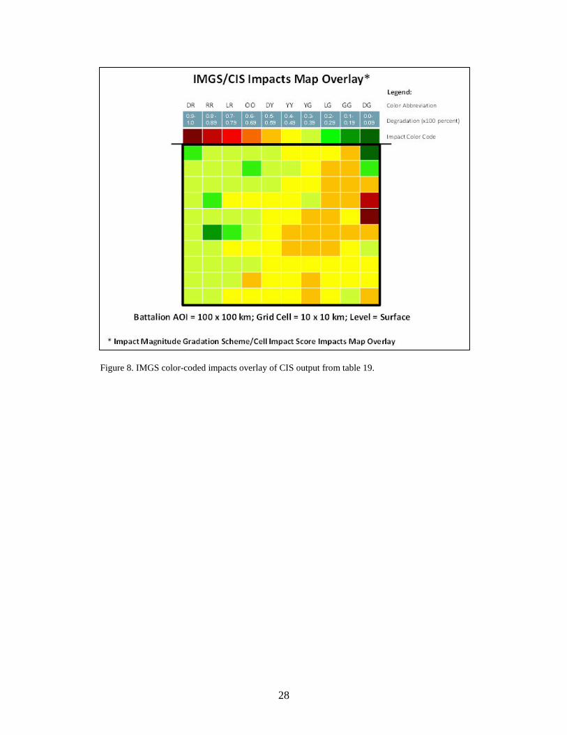
28

Figure 8. IMGS color-coded impacts overlay of CIS output from table 19.

29

Table 20. Excel spreadsheet verification of CIS values.

1 2 3 4 5 6 7 8 9 10

WGTD

Array SUM SUM Position of of

(Row, Col) WND TMP CIG VIS SNO PCP MIVs MIVs CIS (0,0) 0.67 2.12 2.13 0.00 0.33 0.00 5.25 0.88 0.29 (5,0) 0.00 2.12 2.67 0.20 0.11 0.00 5.10 0.85 0.28 (9,0) 0.47 2.09 2.53 0.00 0.33 0.45 5.87 0.98 0.33 (0,4) 0.67 2.07 2.27 0.87 0.56 0.45 6.89 1.15 0.38 (5,4) 0.80 2.02 2.40 1.50 0.00 0.82 7.54 1.26 0.42 (9,4) 1.40 1.12 1.50 1.20 1.67 1.30 8.19 1.37 0.46 (0,9) 1.00 0.00 0.00 0.00 0.00 0.00 1.00 0.17 0.06 (5,9) 1.45 1.07 1.30 1.50 3.00 1.25 9.57 1.60 0.53 (9,9) 1.45 0.91 0.00 2.30 1.33 3.00 8.99 1.50 0.50

Column 1 of table 20 indicates the nine row/column array positions from which the MIVs were taken for each of the six parameters. The MIVs for the six parameters in each array position are listed in columns 2–7. Column 8 is the sum of the MIVs, meaning the equal weighting factor was applied after the MIVs were summed (column 9). In IMGS_FVTDA and in the example shown in table 18, the weighting factor was applied before the MIVs were summed. Since the weighting factor is identical for each of the six parameters (0.1667), the final results are the same. In other words, when the weighting factor is equal for all parameters, the sum-of-the weighted MIVs (as computed by IMGS_FVTDA) is identical to the weighted-sum-of the MIVs (as computed in table 20). Table 20 was arranged in this manner to more clearly show that the correct MIVs are being selected by IMGS_FVTDA and that the final CIS values are accurate. Column 10 is the normalized-sum-of-the-weighted MIVs, i.e., the CIS.

5. Friendly Versus Threat Delta Advantage

It has long been desired to compare weather impacts between Friendly and Threat systems or missions under the same forecast battlefield atmospheric conditions to ascertain which force has the tactical advantage based on the predicted weather (FM 90-22, 1991). Such comparisons were difficult at best with the legacy IWEDA. While it was certainly possible to input a Friendly rules set to IWEDA and then rerun with a separate Threat rules set, side-by-side comparisons of the resulting impact grids were subjective and of limited utility. Since IMGS accounts for (1) how many rules are “firing,” (2) how heavily weighted the weather parameters are, and (3) “threshold exceeding”—and since it produces grids of floating point CIS values, it became possible to quantitatively assess Friendly or Threat weather impacts advantage. To accomplish this, the third

30

phase of the QWI has been developed, which is called Friendly Versus Threat Delta Advantage (FVTDA).

The FVTDA code runs IMGS on a set of Friendly threshold values and then on a separate set of Threat threshold values; it then differences the resulting CIS grids. The same forecast values are input for both sets of MIV/CIS computations. The FVTDA grid is found by computing Threat CIS minus Friendly CIS. If the Threat CIS is larger (indicating a greater weather impact on the Threat system/mission) a positive FVTDA cell value will then result. By differencing in this way, a positive FVTDA value is indicative of a Friendly advantage due to weather impacts in a particular cell. Of course, the converse is true; negative FVTDA values indicate a Threat advantage (or Friendly disadvantage) within the cell. Because the FVTDA values are differences between CIS values, it became necessary to devise a separate color-coding scheme for these results. After several FVTDA runs using realistic sets of Friendly and Threat thresholds, a seven-color scale was applied. Three shades of green indicate Friendly advantage (positive FVTDA values), three shades of red indicate Threat advantage (negative FVTDA values), and gray indicates neutral advantage. This FVTDA color-coding scheme and scale is defined in figure 9 and graphically shown in figures 10 and 11. Note in figure 9 the subtle difference in the breakpoints defining the degree of Friendly advantage versus the degree of Friendly disadvantage (or Threat advantage). We are slightly understating our (Friendly) advantage and slightly overstating the Threat advantage at the breakpoints to reflect our conservative philosophy to error on the side of caution.

Figure 9. FVTDA definitions and criteria for degree of Friendly advantage and disadvantage (or Threat advantage) showing ∆CIS breakpoints and ranges with associated color coding.

31

Figure 10. Graphical representation of the ∆CIS color-code scheme over the range of advantage/disadvantage categories as defined in figure 9.

Figure 11. Representation of the ∆CIS color-code scheme for the degree of Friendly advantage

32

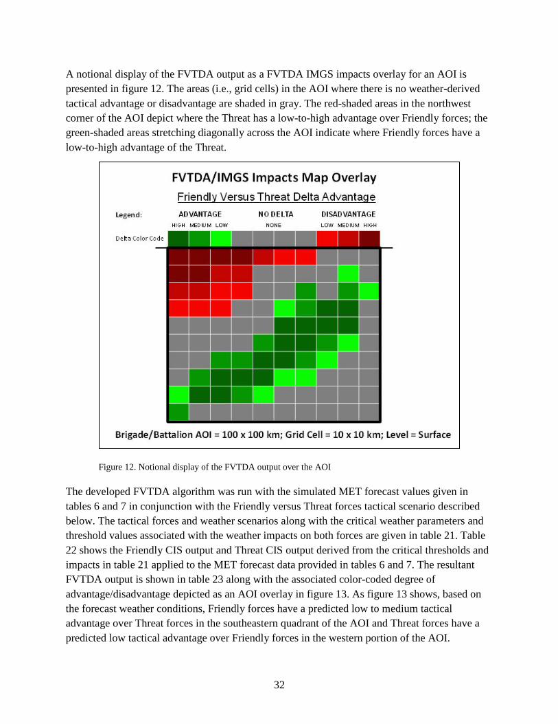
A notional display of the FVTDA output as a FVTDA IMGS impacts overlay for an AOI is presented in figure 12. The areas (i.e., grid cells) in the AOI where there is no weather-derived tactical advantage or disadvantage are shaded in gray. The red-shaded areas in the northwest corner of the AOI depict where the Threat has a low-to-high advantage over Friendly forces; the green-shaded areas stretching diagonally across the AOI indicate where Friendly forces have a low-to-high advantage of the Threat.

Figure 12. Notional display of the FVTDA output over the AOI

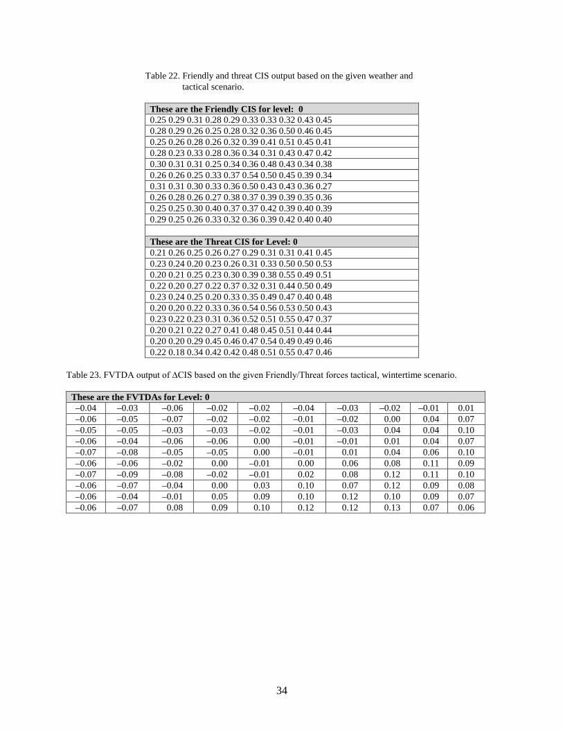
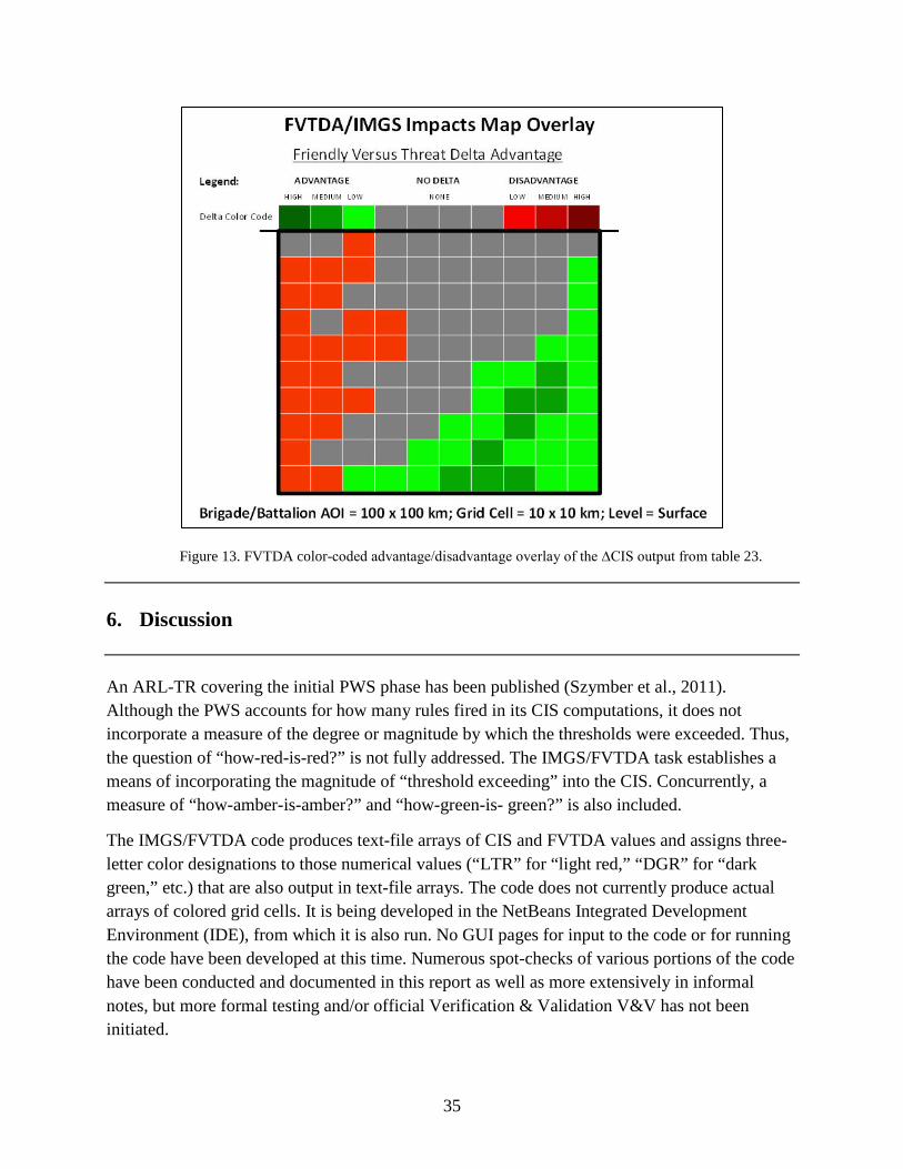
The developed FVTDA algorithm was run with the simulated MET forecast values given in tables 6 and 7 in conjunction with the Friendly versus Threat forces tactical scenario described below. The tactical forces and weather scenarios along with the critical weather parameters and threshold values associated with the weather impacts on both forces are given in table 21. Table 22 shows the Friendly CIS output and Threat CIS output derived from the critical thresholds and impacts in table 21 applied to the MET forecast data provided in tables 6 and 7. The resultant FVTDA output is shown in table 23 along with the associated color-coded degree of advantage/disadvantage depicted as an AOI overlay in figure 13. As figure 13 shows, based on the forecast weather conditions, Friendly forces have a predicted low to medium tactical advantage over Threat forces in the southeastern quadrant of the AOI and Threat forces have a predicted low tactical advantage over Friendly forces in the western portion of the AOI.

33

Table 21. Friendly and threat CIS output based on the given weather and tactical scenario.

Friendly Versus Threat Delta Advantage (FVTDA) Friendly Versus Threat Forces

Ground Maneuver Operations Scenario

1. Tactical Scenario: Friendly Force = US Army weapons/systems and doctrine; Threat Force = Russian/Chinese weapons/systems and doctrine.

2. Weather Scenario: Polar–Winter w/ extreme cold and snow storm conditions.

3. Critical Weather Parameters: temperature, visibility, wind speed, cloud ceiling, precipitation (rain/snow), and snow depth.

4. Forecast Model Assumptions: Level = surface; Grid/Cell size = 10 × 10 km (horizontal resolution); Domain size = 100 × 100 km (AOI).

5. Friendly Force weather effects critical threshold values and impacts: (a) Surface Temperature ≥122 °F {RED} and Surface Temperature >100 °F {AMBER}

Surface Temperature ≤ –40 °F {RED} and Surface Temperature < –20 °F {AMBER}

(b) Visibility <1000 m {RED} and Visibility ≤2000 m {AMBER}

(c) Surface Wind Speed ≥35 kt {RED} and Surface Wind Speed >20 kt {AMBER}

(d) Cloud Ceiling ≤1000 ft {RED} and Cloud Ceiling <2000 ft {AMBER}

(e) Rain/Snow ≥0.3 in/h {RED} and Rain/Snow >0.1 in/h {AMBER} (f) Snow Depth >20 in {RED} and Snow Depth >8 in {AMBER}

6. Threat Force weather effects critical threshold values and impacts: (a) Surface Temperature ≥110 °F {RED}and Surface Temperature > 90 °F {AMBER}

Surface Temperature ≤ –60 °F {RED} and Surface Temperature < –40 °F {AMBER}

(b) Visibility <2,000 m {RED} and Visibility ≤3,000 m {AMBER}

(c) Surface Wind Speed ≥40 kt {RED} and Surface Wind Speed >25 kt {AMBER}

(d) Cloud Ceiling ≤1,500 ft {RED} and Cloud Ceiling <2,500 ft {AMBER}

(e) Rain/Snow ≥0.2 in/h {RED} and Rain/Snow >0.1 in/h {AMBER}

(f) Snow Depth >30 in {RED} and Snow Depth >12 in {AMBER}

34

Table 22. Friendly and threat CIS output based on the given weather and tactical scenario.

These are the Friendly CIS for level: 0 0.25 0.29 0.31 0.28 0.29 0.33 0.33 0.32 0.43 0.45 0.28 0.29 0.26 0.25 0.28 0.32 0.36 0.50 0.46 0.45 0.25 0.26 0.28 0.26 0.32 0.39 0.41 0.51 0.45 0.41 0.28 0.23 0.33 0.28 0.36 0.34 0.31 0.43 0.47 0.42 0.30 0.31 0.31 0.25 0.34 0.36 0.48 0.43 0.34 0.38 0.26 0.26 0.25 0.33 0.37 0.54 0.50 0.45 0.39 0.34 0.31 0.31 0.30 0.33 0.36 0.50 0.43 0.43 0.36 0.27 0.26 0.28 0.26 0.27 0.38 0.37 0.39 0.39 0.35 0.36 0.25 0.25 0.30 0.40 0.37 0.37 0.42 0.39 0.40 0.39 0.29 0.25 0.26 0.33 0.32 0.36 0.39 0.42 0.40 0.40 These are the Threat CIS for Level: 0 0.21 0.26 0.25 0.26 0.27 0.29 0.31 0.31 0.41 0.45 0.23 0.24 0.20 0.23 0.26 0.31 0.33 0.50 0.50 0.53 0.20 0.21 0.25 0.23 0.30 0.39 0.38 0.55 0.49 0.51 0.22 0.20 0.27 0.22 0.37 0.32 0.31 0.44 0.50 0.49 0.23 0.24 0.25 0.20 0.33 0.35 0.49 0.47 0.40 0.48 0.20 0.20 0.22 0.33 0.36 0.54 0.56 0.53 0.50 0.43 0.23 0.22 0.23 0.31 0.36 0.52 0.51 0.55 0.47 0.37 0.20 0.21 0.22 0.27 0.41 0.48 0.45 0.51 0.44 0.44 0.20 0.20 0.29 0.45 0.46 0.47 0.54 0.49 0.49 0.46 0.22 0.18 0.34 0.42 0.42 0.48 0.51 0.55 0.47 0.46

Table 23. FVTDA output of ∆CIS based on the given Friendly/Threat forces tactical, wintertime scenario.

These are the FVTDAs for Level: 0 –0.04 –0.03 –0.06 –0.02 –0.02 –0.04 –0.03 –0.02 –0.01 0.01 –0.06 –0.05 –0.07 –0.02 –0.02 –0.01 –0.02 0.00 0.04 0.07 –0.05 –0.05 –0.03 –0.03 –0.02 –0.01 –0.03 0.04 0.04 0.10 –0.06 –0.04 –0.06 –0.06 0.00 –0.01 –0.01 0.01 0.04 0.07 –0.07 –0.08 –0.05 –0.05 0.00 –0.01 0.01 0.04 0.06 0.10 –0.06 –0.06 –0.02 0.00 –0.01 0.00 0.06 0.08 0.11 0.09 –0.07 –0.09 –0.08 –0.02 –0.01 0.02 0.08 0.12 0.11 0.10 –0.06 –0.07 –0.04 0.00 0.03 0.10 0.07 0.12 0.09 0.08 –0.06 –0.04 –0.01 0.05 0.09 0.10 0.12 0.10 0.09 0.07 –0.06 –0.07 0.08 0.09 0.10 0.12 0.12 0.13 0.07 0.06

35

Figure 13. FVTDA color-coded advantage/disadvantage overlay of the ∆CIS output from table 23.

6. Discussion

An ARL-TR covering the initial PWS phase has been published (Szymber et al., 2011). Although the PWS accounts for how many rules fired in its CIS computations, it does not incorporate a measure of the degree or magnitude by which the thresholds were exceeded. Thus, the question of “how-red-is-red?” is not fully addressed. The IMGS/FVTDA task establishes a means of incorporating the magnitude of “threshold exceeding” into the CIS. Concurrently, a measure of “how-amber-is-amber?” and “how-green-is- green?” is also included.

The IMGS/FVTDA code produces text-file arrays of CIS and FVTDA values and assigns three-letter color designations to those numerical values (“LTR” for “light red,” “DGR” for “dark green,” etc.) that are also output in text-file arrays. The code does not currently produce actual arrays of colored grid cells. It is being developed in the NetBeans Integrated Development Environment (IDE), from which it is also run. No GUI pages for input to the code or for running the code have been developed at this time. Numerous spot-checks of various portions of the code have been conducted and documented in this report as well as more extensively in informal notes, but more formal testing and/or official Verification & Validation V&V has not been initiated.

36

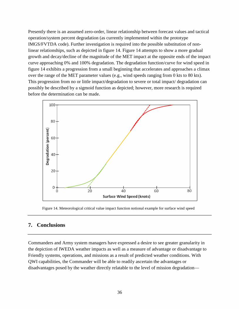
Presently there is an assumed zero-order, linear relationship between forecast values and tactical operation/system percent degradation (as currently implemented within the prototype IMGS/FVTDA code). Further investigation is required into the possible substitution of non-linear relationships, such as depicted in figure 14. Figure 14 attempts to show a more gradual growth and decay/decline of the magnitude of the MET impact at the opposite ends of the impact curve approaching 0% and 100% degradation. The degradation function/curve for wind speed in figure 14 exhibits a progression from a small beginning that accelerates and approaches a climax over the range of the MET parameter values (e.g., wind speeds ranging from 0 kts to 80 kts). This progression from no or little impact/degradation to severe or total impact/ degradation can possibly be described by a sigmoid function as depicted; however, more research is required before the determination can be made.

Figure 14. Meteorological critical value impact function notional example for surface wind speed

7. Conclusions

Commanders and Army system managers have expressed a desire to see greater granularity in the depiction of IWEDA weather impacts as well as a measure of advantage or disadvantage to Friendly systems, operations, and missions as a result of predicted weather conditions. With QWI capabilities, the Commander will be able to readily ascertain the advantages or disadvantages posed by the weather directly relatable to the level of mission degradation—

37

considering both Friendly and Threat capabilities and providing for a more meaningful four-dimensional assessment of battlefield weather effects over time and space.

This report describes the development and use of a new IMGS and FVTDA capability applied to the IWEDA decision support tool. A ten-step color code is assigned based on the magnitude of the impacts for the IMGS; and for the FVTDA, a seven-step color code is assigned to reflect the magnitude of advantage or disadvantage Friendly forces have with respect to Threat forces based on the forecast weather conditions. The IMGS provides a capability for the first time of quantifying the output of IWEDA rules’ degree of impact by computing a composite impact score that to a certain extent portrays “how red is red,” “how amber is amber,” or “how green is green.”

The IMGS and FVTDA models are directed toward extending the PWS concept to account for how much the thresholds are being exceeded by the forecast values. IMGS will provide a capability to fully answer the questions of “how red is red?” and so forth. Also, the FVTDA provides a capability is to produce separate CIS arrays for “Friendly” and “Threat” mission or counter-mission areas. By differencing these arrays it will then be possible to assess whether US and coalition forces will hold the advantage over the enemy on the battlefield in terms of the severity of adverse weather impacts. The IMGS and FVTDA (along with the previously developed PWS) will be able to enhance the functionality and maximize the inherent capabilities of the next generation of IWEDA, called My Weather Impacts Decision Aid (MyWIDA) currently under development by ARL.

38

INTENTIONALLY LEFT BLANK.

39

8. References

Department of the Army, Memorandum, Accreditation of Integrated Weather Effects Decision Aid (IWEDA) Software and Associated Rules Database; Deputy Director, Combat Developments, U.S. Army Intelligence Center and Fort Huachuca, AZ, 27 June 2006.

FM 34-81-1. Battlefield Weather Effect; Department of the Army: Washington, DC, 1992.

FM 90-22. (Night) Multiservice Night and Adverse Weather Combat Operations; Department of the Army: Washington, DC, 31 January 1991.

Raby, J.; Szymber, R. J.; Brown, R. Development of a Methodology for Determining the Value-Added of High Temporal and Spatial Resolution Model Weather Forecasts Over Standard Mesoscale Model Weather Forecasts; ARL-TR-3116; U.S. Army Research Laboratory: White Sands Missile, NM, November 2003.

Sauter, D.; Torres, M.; Brandt, J.; McGee, S. The Integrated Weather Effects Decision Aid: A Common Software Tool to Assist in Command and Control Decision Making. Proceedings of the Command & Control Research & Technology Symposium, Newport, RI, 1999.

Szymber, R. J. U. S. Army Tactical Weather Support Requirements for Weather and Environmental Data Elements and Meteorological Forecasts; ARL-TR-3720; U.S. Army Research Laboratory: White Sands Missile Range, NM, February 2006.

Szymber, R. J. U.S. Army Tactical Weather and Environmental Data Requirements, Critical Threshold Values and Impacts on Operations and Systems, and the Integrated Weather Effects Decision Aid (IWEDA) Rules; ARL-TR-4672; U.S. Army Research Laboratory: White Sands Missile Range, NM, December 2008.

Szymber, R. J.; Jameson, T.; Knapp, D. An Integrated Weather Effects Decision Aid Parameter Weighting Scheme; ARL-TR-5570; U.S. Army Research Laboratory: White Sands Missile Range, NM, June 2011.

40

INTENTIONALLY LEFT BLANK.

41

Appendix. IMGS/FVTDA Outline-Flowchart

"IMGS_FTVDA.java" Flowchart Listing

Forecast Model Level Loop

Row/Col Loops

Parameter Loop

Line No. Action NOTES

55-56 Decalre PrintStream object called "cell_scores_file" for "IMGS_results.txt" File for MIVs, CIS's, and FVTDAs

58-59 Declare PrintStream object called "setup_results_file" for "IMGS_setup_results.txt" Output file verifying setup data input

61-62 Declare PrintStream object called "th_m_b_file" for "thresh_slope_incpt.txt" Output file verifying thresh/slp/intcpts

64-65 Declare PrintStream object called "code_dev_file" for "code_dev_prog.txt" Output file logging code development

83-84 Declare Scanner object called "read_setup_file" for "IMGS_input.txt" Input file-domain size/num parameters

85-86 Declare Scanner object called "read_FTV_file" for "FTV.txt" Input for Friendly threshold values

87-88 Declare Scanner object called "read_TTV_file" for "TTV.txt" Input for Threat threshold values

89-90 Declare a Scanner object called "read_FV_file" for "forecast_values.txt" Input for parameter forecast values

96-120 Integer/Double/String declarations

128-129 Declare Decimal Format objects "df_7_4" and "df_4_2"

132-135 Label "thresh_slope_incpt.txt"

148-149 Declare "SetupData" object called "read_write_setup". "read_setup_file", "setup_results_file", and "th_m_b_file" are sent to constructor Object for I/O of setup values

159 Run "read_write_setup.SetupIO" method. Read all setup params. Output to verify

170-179 Assign "read_write_setup" setup attributes to their respective variables with same names in "main" method (eg. 'aoi_r', 'm', etc.)

Array dimensions; max Red IV; medium and light multiplying factors; number of Friendly, Threat, and Fcst Params.

185 Declare "ParamWgts" class "F_pWgts_compute" object Object to compute Friendly param wgts

186 Declare "ParamWgts" class "F_pWgts_compute" object Object to compute Threat param wgts

195 Declare "ForecastArray" class "inputFVs" object Object to read in forecast params arrays

Assign "num_params" as the larger of "num_F_params" or "num_T_params"

This appendix appears in its original form, without editorial change.

42

Run "read_write_setup.CIS_param_compute" method. Computes "num_non_0_wgt_params" and "eq_p_wgt" for both Friendly and Threat and writes to "MIGS_setup_results.txt"

Assign "read_write_setup" attributes "num_non_0_wgt_F_p", "num_non_0_wgt_T_p", "eq_F_p_wgt", and "eq_T_p_wgt" to variables with same name in "main" method

Array declarations

Declare "CIS" class "CIS_compute" object. Send "max_sum_wgt_iv" and "num_non_0_wgt_p" to its constructor.

Declare the "SlopeIntcpt" class object called "FV_IV_line_compute". The "PrintStream" object called "th_m_b_file" is sent to its constructor.

Begin "Friendly" Asset section

377 Read first labeling line of "FTV.txt"

385 Begin Friendly "param" loop

394 Read parameter name

406 Read parameter weighting category string

413 Convert parameter weighting category string to single character called "param_wgt_cat"

414-417 If statements to count "num_h", "num_m", and "num_l"

430 Run the "read_write_setup.thresholdIO" method to read this parameter's threshold values

437-440 Assign "read_write_setup" attributes ("max_R_TH", etc.) to variables in "main" method

451-465

Run the "FV_IV_line_compute.findSlope" method to find the parameter's three line's slopes. Run the "FV_IV_line_compute.findYIntcpt" method to find the parameter's three line's intercepts.

474-475 Run the "FV_IV_line_compute.writeSlopeIntcpt" method to write the three slopes and intercepts to "thresh_slope_incpt.txt"

478 End Friendly "param" loop

484 Run the "pWgts_compute.findParamWgts" method

491-494 Assign "pWgts_compute" attributes ("l_wgt", etc.) to variables in "main" method

496-509 Write "l_wgt", etc. to "MIGS_setup_results.txt" via "setup_results_file" object

522 Begin Friendly "param" loop

524 Run "pWgts_compute.setParamWgts" method toassign each parameter's numerical weight.

526-528 Write each Friendnly parameter's weight to the "thresh_slope_incpt.txt" file

530 Sum individual assigned parameter weights to find total weight called "tot_assgnd_wgt"

43

531 End Friendly "param" loop

534-543 Write the total parameter weight to "MIGS_setup_results.txt". Check for equal to 1.00

553

The empty 4-D forecast value array is sent to the "inputFVs.readFVs" method as an argument. In line 350 "inputFVs" is declared as a "ForecastArray" class object. The "read_FV_file" Scanner object is sent into its constructor. The full "fcst_value" array (all parameters) is returned from this method.

584 Begin "level" loop

587-591 Begin "row", "column" loops

597 Reset "sum_wgt_imp_values" for this next cell equal to zero.

599 Begin Friendly "param" loop

610 Set the "fcst_value [ll] [p] [r] [c]" value equal to simply "FV"

624-687

Check for pos/neg slopes of the FV-MIV line for this parameter. Check "FV" for green, amber, or red line segment. Send the FV, slope, and y-intercept to the "CIS_compute.modImpValue" method to compute the "MIV" for this cell/parameter.

695-697 Check MIV <= max_R_IV. If greater than, set equal to "max_R_IV".

699-701 Check MIV >= 0.0. If less than, set equal to 0.0.

712 Compute the weighted MIV called "wgt_imp_value".

708 Sum the weighted modified impact values, parameter by parameter.

720-745 These lines of code have a commented section that outputs the FV, slope, y-intercept, and MIV for a single cell and parameter. These data are output to the command line.

745 End Friendly "param" loop

751 Send "sum_wgt_imp_values" to the "CIS_compute.find_CIS_nswiv" method to compute the Friendly CIS for this cell (called "F_CIS").

753-755 End "column" and "row" loops

757-759 Skip down in "MIGS_results.txt" for output of the next level.

786 Begin Friendly "param" loop

789-791 Print labeling to "cell_scores_file" PrintStream object

794 Send Friendly "mod_impact_value" array to "print4DArray" static method for output

797 End Friendly "param" loop

799-800 Skip down in "MIGS_results.txt" for output of "F_CIS" values.

820 Write "F_CIS" labeling to output file

826 Send "F_CIS" array to "print3DArray" static method for output

828 Skip down in "MIGS_results.txt" for output of "F_CIS" colors.

831 Write "F_CIS" grid color labeling to "MISG_results.txt"

837 Send "F_CIS" array to "printCISColors" static method for output

842-844 Skip down in "MIGS_results.txt" for output of next level of data.

847 End of "level" loop

End "Friendly" Asset section

44

Begin "Threat" Asset section

865 Read first labeling line of "TTV.txt"

870 Reset "tot_assgnd_wgt" equal to 0.0

875 Begin Threat "param" loop

878 Read parameter name

883 Read parameter weighting category string

888 Convert parameter weighting category string to single character called "param_wgt_cat"

894 Run "pWgts_compute.setParamWgts" method to find numerical parameter weight

899-901 Write labeling to "thresh_slope_incpt.txt"

907 Sum individual parameter weights to find total weight called "tot_assgnd_wgt"

913 Run the "read_write_setup.thresholdIO" method to read this parameter's threshold values

919-922 Assign "read_write_setup" attributes ("max_R_TH", etc.) to variables in "main" method

928-946

Run the "FV_IV_line_compute.findSlope" method to find the parameter's three line's slopes. Run the "FV_IV_line_compute.findYIntcpt" method to find the parameter's three line's intercepts.

955-956 Run the "FV_IV_line_compute.writeSlopeIntcpt" method to write the three slopes and intercepts to "thresh_slope_incpt.txt"

960 End Threat "param" loop

963-971 Write the total parameter weight to "MIGS_setup_results.txt". Check for equal to 1.00

977 Begin "level" loop

980-984 Begin "row", "column" loops

990 Reset "sum_wgt_imp_values" for this next cell equal to zero.

992 Begin Threat "param" loop

995 Set the "fcst_value [ll] [p] [r] [c]" value equal to simply "FV"

1002-1065

Check for pos/neg slopes of the FV-MIV line for this parameter. Check "FV" for green, amber, or red line segment. Send the FV, slope, and y-intercept to the "CIS_compute.modImpValue" method to compute the "MIV" for this cell/parameter.

1070-1072 Check MIV <= max_R_IV. If greater than, set equal to "max_R_IV".

1074-1076 Check MIV >= 0.0. If less than, set equal to 0.0.

1082 Compute the weighted MIV called "wgt_imp_value".

1084 Sum the weighted modified impact values, parameter by parameter.

1087 End Threat "param" loop

1093-1110 These lines of code allow output of the FV, MIV, and parameter name for a single cell and parameter to spot-check the data. These data are output to the command line.

45

1121 Send "sum_wgt_imp_values" to the "CIS_compute.find_CIS_nswiv" method to compute the Threat CIS for this cell (called "T_CIS").

1128 Difference the "F_CIS" from the "T_CIS" for this cell to find its "FVTDA"

1130-1132 End "column" and "row" loops

1139 Begin Threat "param" loop

1142-1144 Print Threat MIVs labeling to "cell_scores_file" PrintStream object

1146 Send Threat "mod_impact_value" array to "print4DArray" static method for output

1147 End Threat "param" loop

1149-1151 Print "T_CIS" labeling to "cell_scores_file" PrintStream object

1153 Send "T_CIS" array to "print3DArray" static method for output

1156-1158 Print "FVTDA" labeling to "cell_scores_file" PrintStream object

1160 Send "FVTDA" array to "print3DArray" static method for output

1162 End of "level" loop

46

INTENTIONALLY LEFT BLANK.

47

List of Symbols, Abbreviations, and Acronyms

AOI Area of Interest

ARL U.S. Army Research Laboratory

CIG cloud ceiling

CIS Cell Impact Score

CRDB Centralized Rules Data Base

FV forecast value

FVTDA Friendly Versus Threat Delta Advantage

IDE Integrated Development Environment

IMETS Integrated Meteorological System

IMGS Impact Magnitude Gradation Scheme

IV Impact Value

IWEDA Integrated Weather Effects Decision Aid

MET Meteorological

MIV modified impact value

MyWIDA My Weather Impacts Decision Aid

NWP Numerical Weather Prediction

PCP precipitation rate

PWS Parameter Weighting Scheme

QWI Quantitative Weather Impacts

S_W_MIV Sum of the Weighted Modified Impact Values

slp slope

SNO snow depth

TMP temperature

V&V Verification & Validation

48

VIS visibility

W_MIV Weighted Modified Impact Values

WSP wind speed

y-int y-axis intercept point

WSP Wind Speed

49

No. of Copies Organization

1 DEFENSE TECHNICAL (PDF) INFORMATION CTR DTIC OCA 2 DIRECTOR

(PDFS) US ARMY RSRCH LAB RDRL CIO LL RDRL IMAL HRA

RECORDS MGMT 1 GOVT PRINTG OFC (PDF) A MALHOTRA 7 US ARMY RSRCH LAB (PDFs) ATTN RDRL CIE M T C JAMESON R J SZYMBER D I KNAPP J O JOHNSON ATTN RDRL CIE D S G O’BRIEN ATTN RDRL CIE P A CLARK J L COGAN

50

INTENTIONALLY LEFT BLANK.