quantitative surface characterisation using laser scanning confocal microscopy

1

Quantitative Surface Characterisation Using Laser Scanning Confocal Microscopy

Steven Tomovich1, Zhongxiao Peng1, Chengqing Yuan2 and Xinping Yan2 1School of Engineering & Physical Sciences

James Cook University, Queensland, 2Reliability Engineering Institute, School of Energy and Power Engineering

Wuhan University of Technology, Wuhan, 1Australia

2China

1. Introduction

This chapter reports the development of a new quantitative surface characterisation system

based on laser scanning confocal microscopy (LSCM). This development involves:

systemically studying and understanding the resolutions of a LSCM and its capacity;

investigating appropriate hardware settings for acquiring suitable two-dimensional (2D)

images; assess image processing techniques for eliminating noise and artefacts while

constructing three-dimensional (3D) images for quantitative analysis; and developing

quantitative image analysis techniques to characterise the required features of surfaces. This

chapter will show examples of using a LSCM for image acquisition and the developed

techniques for the surface characterisation of engineering surfaces and wear particles in

engineering and bioengineering applications.

2. Importance

Quantitative surface characterisation is an essential and common practice in many

applications. Two-dimensional surface measurement has been performed for over 50 years

using traditional 2D surface roughness parameters including the arithmetic mean deviation

(Ra), root mean squared deviation (Rq), surface skewness (Rsk) and surface kurtosis (Rku), etc

that are based on single line surface traces (Gadelmawla et al., 2002). The technique has been

popularly used to measure large surfaces in 2D. Standard 2D measurements are commonly

performed using the stylus profiler that traces a diamond stylus tip over the specimen

surface, recording vertical displacement over distance travelled (DeGarmo, 1997). The

resolution of the system is governed by the stylus tip size selected for testing surfaces of

specific material type and surface finish. However, in operation the stylus unfortunately

subjects the surface to damage (Bennett and Mattsson, 1989; Gjonnes, 1996; Conroy and

Armstrong, 2005) and thus the technique cannot be used to perform surface measurement

on soft materials. In addition, the minimum scan length for the stylus technique (ISO

standards 4288, 1996) is not suited to small wear particle surfaces.

www.intechopen.com

Laser Scanning, Theory and Applications

2

Due to the complexity of surface topography, the extraction of surface roughness information in 3D is often required for the accurate characterisation of surface features. Standard scanning electron microscopy (SEM) has been extensively used for characterising surface features. Scanning electron microscopy has outstanding 2D resolution and with specialised SEM operation can also provide 3D images (Podsiadlo and Stachowiak 1997; Bernabeu et al., 2001). However, in addition to the specialised preparation time required, the fact samples are modified during preparation and possibly during image acquisition are issues to consider when using SEM (Brown and Newton, 1994; Chescoe and Goodhew, 1990; Hanlon et al., 2001). Atomic force microscopy (AFM) is a technique often used for 3D surface measurement that is to a degree non-contacting or destructive, while also possessing sub nanometre resolution in 3D. The limitation with this technique is the maximum scan

area of ≈100 μm2 that is not sufficient for the study of some surfaces (Gauldie et al., 1994; Martin et al., 1994; Conroy and Armstrong, 2005). A non-destructive and versatile technique for characterising surface information in 3D is the LSCM imaging system. This technique involves sequentially illuminating the focal plane with a diffraction-limited light spot point by point. Specimen information is transmitted back through the optics via a confocal aperture as a diffraction-limited spot to reduce light from above and below focal plane. The sharpened light spot is converted into an electrical signal by the photo multiplier tube (PMT) point detector and then digitised for storage or display. By sequentially scanning through the specimen field of view, a 2D digital image of the focal plane is formed. The significant benefit over standard optical microscopy is the LSCM ability to discriminate between in focus and out of focus light above and below the focal plane. In addition to imaging high-resolution 2D slices from the focal plane, another primary feature is the system’s ability to capture 3D images. By compiling a series of adjacent 2D digital images captured at different heights in the specimen, constructed 3D images provide 3D surface and volume information by a non-contacting and un-intrusive method (Sheppard and Shotton, 1997; Pawley, 1995). Using specialised software, surface measurements can be readily performed on variations in pixel intensity and spatial locations contained in 3D images (Brown and Newton, 1994; Yuan et al., 2005). By comparison the resolution of LSCM is possibly higher than a standard stylus profiler and can non-intrusively obtain surface information from large and small surfaces in 3D while the stylus profiler is restricted to measuring surface characteristics of large surfaces in 2D. The confocal system also provides a greater field of view and depth range than AFM, which is more suitable for industrial surfaces measurements. In addition, the minimal specimen preparation for LSCM imaging sets the technique to be a fast and versatile instrument for quantitative surface measurements (King and Delaney, 1994; Gjonnes, 1996; Bernabeu et al., 2001; Sheppard and Shotton, 1997; Haridoss et al., 1990). Past research using traditional 2D parameters for quantitative surface analysis found good correlation between roughness measurements of metal surfaces determined by LSCM, stylus and AFM surface measurement techniques (Gjonnes, 1996; Hanlon et al., 2001; Peng and Tomovich, 2008). Early research and development of surface measurement using LSCM found the technique to be viable for extracting surface information from 3D images in the form of numerical parameters, calculated from images generated using height encoded image (HEI) processing techniques (Peng and Kirk, 1998 & 1999). However, developments are still in their infant stages. The aim of this presented study is to develop a set of techniques so that LSCM can be used widely for quantitative surface characterisation in 3D for a range of studies and applications.

www.intechopen.com


3

Specifically, this project involves the evaluation of the LSCM resolution and imaging system performance in relation to hardware parameter settings; the establishment of correct procedures for acquiring high quality images for quantitative 3D surface measurements and the development and validation of the 3D LSCM surface measurement technique. The details of the above developments are presented in the following section.

3. Development of 3D imaging, processing and analysis techniques for quantitative surface measurement

Surface measurement using any image acquisition systems involves three major steps, namely, data acquisition, processing and analysis. As this project is to develop 3D surface measurement techniques based on laser scanning confocal microscopy, the developments have been conducted in the following four phases. Phase 1 is to evaluate the LSCM system and to perform resolution testing to determine the optimal system settings for the acquisition of high quality images for numerical analysis. Phase 2 involves image processing to construct 3D images using acquired 2D image sets and to eliminate image artefacts and distortion. Phase 3 focuses on the development and selection of numerical parameters for surface measurement, and Phase 4 involves testing and validating the techniques using various samples. The section presents our research and developments on phases 1, 2 and 4.

3.1 Laser scanning confocal microscope resolution testing A comprehensive study of the image acquisition system performance and resolutions has

been conducted. To extract meaningful surface information from raw 3D images, the

performance of the Radiance2000 LSCM imaging system and specimen influences on the

image formation process must be fully understood to bring to light what is real

morphological surface information or simply specimen and imaging system related artefact.

It is for this reason that image acquisition tests focused on imaging metallic surfaces of

known morphology and reflectivity.

For the tested objective lens, images of a front coated aluminium optical flat (Edmunds

Optics 43402) were captured over several increments of scan rate, laser power, PMT gain,

Kalman frame averaging and confocal aperture setting using zoom 999. Height encoding

(Sheppard and Matthews, 1987; Pawley, 1995; Peng and Tomovich, 2008) the raw LSCM

3D images created HEI containing minimum and maximum z positions used to determine

HEI depth. Plotted against increasing parameter settings, HEI depth highlighted the

variance in depth discrimination (axial resolution) with various LSCM settings. Also

useful in studying image quality were 2D maximum brightness images (MBI) constructed

from raw 3D images with HEI. The coefficient of variance (CV) calculated from the

standard deviation (SD) and mean pixel intensity (u) of MBI, provided a measure of

image noise (Zucker and Price, 2001) that were plotted against LSCM settings. To visually

assess the lateral resolution of lenses, chromium graticule and bar structures on the Gen

III Richardson test slide were imaged using Nyquist zoom. Contrast measured

(Oldenbourg et al., 1993; Pawley, 1995) across the structures and plotted against scan rate,

frame averaging and aperture settings also highlighted the influence of these parameters

on lateral resolution. For each objective lens, limiting HEI axial and lateral resolutions

achieved for metrology applications were then determined from optical flat HEI depth

tests and HEI of structures on the Richardson slide.

www.intechopen.com


4

Scan Rate Testing

Using a Nikon LU Plan 100x lens, original tests for scan rate over the 166-750 Hz range produced HEI depths in Figure 1a that show the 600 Hz to provide the highest depth discrimination. Measured depths were expected to increase with image noise reflected by increasing CV in Figure 1b. When comparing Figures 1a original scan and Figure 1b, no clear relationship exists between increasing image noise and original HEI depths that were found to be impacted on by scanning distortions. However, depth discrimination was shown to reduce with increasing scan rate for the modified plot in Figure 1a on removing the distortions prior to height encoding.

HEI Depth versus Scan Rate

( Distortion removed )

11.0

60 n

m

9.62

3 nm

10.1

97 n

m

6.94

3 nm

166H

z

500H

z

600H

z 750H

z

5

10

15

20

25

30

35

150 250 350 450 550 650 750

Scan Rate ( Hz )

HE

I D

ep

th (

nm

)

Distortion Removed Original Scan

HE

I d

epth

( n

m )

Scan Rate ( Hz )

( a ) Coefficient of Variance

versus Scan Rate

750H

z

500H

z

600H

z

166H

z

1%

2%

2%

3%

3%

4%

4%

5%

5%

150 250 350 450 550 650 750

Scan Rate ( Hz )

Co

effic

ien

t o

f V

ari

an

ce

( C

V )

Co

effi

cien

t o

f V

ari

an

ce (

CV

)

Scan Rate ( Hz )

( b )

Fig. 1. Depth discrimination reduced with higher scan rates (a) as maximum brightness image noise increases (b).

Evidence of scanning distortion in Figures 2a-d show waves unique to each scan rate traversing left to right in sections from the full HEI representing a single optical flat location. The distortion potentially stems from mechanical instability in the galvanometer driving the left to right horizontal scanning process. In sections taken from the left side of the full HEI, Figures 3a-d show an increased waviness of scan lines due to the vertical scanning process traversing from top to bottom in the 500-750 Hz HEI. When comparing Figures 3a-d for image tilt, the 166 Hz HEI slope down towards the bottom of the image while faster scan rates show little tilt for the same optical flat location. This was present in all 166 Hz HEI indicating depths in Figure 1 for the 166 Hz original scan, included the effects of the stage drifting in the z direction with extended imaging time. Comparing HEI over increasing scan rate in both Figures 2-3, there is a slightly higher level of graininess in HEI for the 500-750 Hz scan rates. To clearly associate increasing MBI noise reflected by CV in Figure 1b with increasing graininess of HEI and reduced depth discrimination, scanning distortions were therefore minimised in raw 3D data prior to height encoding. This was achieved by cropping images using the Radiance2000 LSCM operating system software LaserSharp2000, to provide five separate 252 xy pixel framed 3D image series. By reducing the sampling area the distortions traversing left to right were selectively filtered out and the tilt component substantially minimised, placing more significance on HEI depth associated with graininess. In a practical sense, the scale of

www.intechopen.com


5

(x)

(y)

20 nm

( a ) 166 Hz HEI

( b ) 500 Hz HEI

( c ) 600 Hz HEI

( d ) 750 Hz HEI

Fig. 2. Traversing left-right the (a) 166 Hz, (b) 500 Hz, (c) 600 Hz & (d) 750 Hz height encoded image distortions.

( a ) 166 Hz HEI ( b ) 500 Hz HEI ( c ) 600 Hz HEI ( d ) 750 Hz HEI

(x)

(y)

20 nm

Fig. 3. Stage drift that increased the 166 Hz HEI depth (a) and scan line waviness increasing for the 500-750 Hz HEI (b-d).

www.intechopen.com


6

distortions found in HEI are minimal when using Nyquist zoom and the cropping of images to remove their effect served only to assess parameter settings during preliminary tests. Although the modified HEI depths in Figure 1a now increase with CV in Figure 1b, the proportion image noise contributed to total HEI depth still remains unknown. Further, scan area geometric error and xy translational error of the stage will also introduce an unknown degree of shift in the optical flat surface that will impact on HEI depth. However, given these limitations the height encoding test did provide a more direct assessment of image quality and therefore remained a key indicator for LSCM testing. To establish an ideal scan rate it was also necessary to assess the impact of scan rate on lateral resolution, defined as the minimum separating distance for two points to remain resolved with some level of contrast (Pawley, 1995). The standard test involves direct imaging of finely spaced graticule structures to visually assess limitations in lateral resolution. Extracting pixel intensities across the MBI of structures exampled in Figure 4a produced the intensity profile over x or y distance in microns. The contrast measured between the minimum and maximum profile intensities diminish with finer graticule spacing, or as in case with increasing image noise due to using higher scan rates. Imaging both vertical and horizontal 0.25 µm metal graticules on the Richardson test slide provided measured contrast versus scan rate in Figure 4b for the 100x lens. For the 166-750 Hz scan rates vertical contrast measured 10.34%, 11.32%, 15.50% and 25.17% more across horizontal graticules than across vertical graticules. The difference indicates a more symmetric lateral resolution was achieved using the 166-500 Hz scan rates. The reduced horizontal and increased vertical contrast for the 600-750 Hz scan rates, stems from the scanning and digitisation process that is continuous from left to right and discontinuous in the vertical. Scanning left to right, the continuous PMT output signal is digitised sequentially and appears to have generated a smearing of pixel intensities when scanning across passing differences in surface reflectivity. Circled in Figure 4c, the 750 Hz MBI of 2-4 µm horizontal graticules show smearing of pixel intensity across the non reflective substrate that is likely caused by some form of lag in PMT response. Graticules aligned perpendicular to the

Fig. 4. Intensities data extracted across 0.25 µm vertical graticules (a), the impact of scan rate on measured contrast (b) and the carry over of reflection signal across the substrate regions when using the 750 Hz scan rate (c).

Line Intensity Profile

( 0.25 μm graticules )

0

50

100

150

200

250

0.0 0.5 1.0 1.5 2.0 2.5 3.0 3.5 4.0 4.5 5.0 5.5 6.0

Distance-xy ( μm )

Pix

el In

ten

sity (

Gre

y le

ve

ls

Pix

el I

nte

nsi

ty (

Gre

y l

evel

s )

Distance-x ( µm )

Extracted pixel intensities

( a ) Contrast versus Scan Rate

( 0.25 um graticules )

166H

z

600H

z

500H

z

750H

z

40%

45%

50%

55%

150 250 350 450 550 650 750

Scan Rate ( Hz )

Co

ntr

ast (%

)

Horizontal graticules

Vertical graticules

750Hz MBI

Co

ntr

ast

( %

)

Scan Rate ( Hz )

( b ) ( c )

www.intechopen.com


7

continuous scan direction, suffered reduced contrast and subsequent resolution due to the elevated signal from the substrate regions. Horizontally aligned graticules experienced a reinforcing of brightness for the reflective metal strips with no carry over signal across the substrate, overall increasing vertical contrast for the 600-750 Hz. Although the 166Hz scan rate provided the highest axial resolution with the most symmetric lateral resolution, engineering surfaces often have deep structures in addition to surface form and tilt that add significantly to the depth of a 3D image series. When imaging extended surfaces with the 166 Hz, acquisition time rapidly increases with the number of sections. The most practical scan rates for large image series are the 500-750 Hz that also eliminates stage drift in the z direction. For the 750Hz, pixel smearing and the excessive graininess of HEI need to be considered when imaging finer structures.

Laser Power and PMT Gain

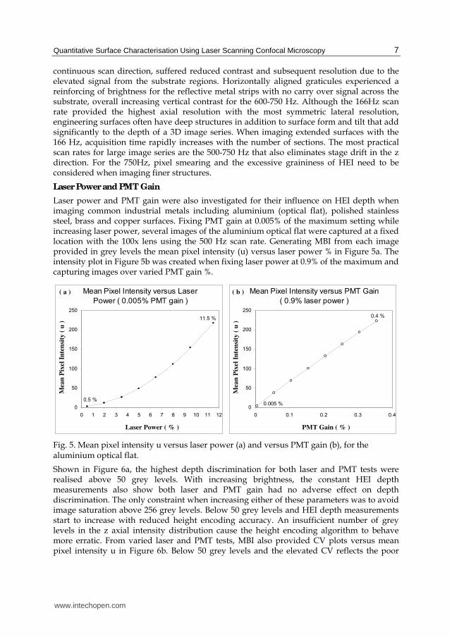
Laser power and PMT gain were also investigated for their influence on HEI depth when imaging common industrial metals including aluminium (optical flat), polished stainless steel, brass and copper surfaces. Fixing PMT gain at 0.005% of the maximum setting while increasing laser power, several images of the aluminium optical flat were captured at a fixed location with the 100x lens using the 500 Hz scan rate. Generating MBI from each image provided in grey levels the mean pixel intensity (u) versus laser power % in Figure 5a. The intensity plot in Figure 5b was created when fixing laser power at 0.9% of the maximum and capturing images over varied PMT gain %.

Mean Pixel Intensity versus Laser

Power ( 0.005% PMT gain )

11.5 %

0.5 %

0

50

100

150

200

250

0 1 2 3 4 5 6 7 8 9 10 11 12

Laser Power ( % )

Mean

Pix

el In

tensity ( μ

)

Mean Pixel Intensity versus PMT Gain

( 0.9% laser power )

0.4 %

0.005 %0

50

100

150

200

250

0 0.1 0.2 0.3 0.4

PMT Gain ( % )

Mean

Pix

el In

tensity ( μ

)M

ean

Pix

el I

nte

nsi

ty (

u )

PMT Gain ( % )

( b )

Mea

n P

ixel

In

ten

sity

( u

)

Laser Power ( % )

( a )

Fig. 5. Mean pixel intensity u versus laser power (a) and versus PMT gain (b), for the aluminium optical flat.

Shown in Figure 6a, the highest depth discrimination for both laser and PMT tests were realised above 50 grey levels. With increasing brightness, the constant HEI depth measurements also show both laser and PMT gain had no adverse effect on depth discrimination. The only constraint when increasing either of these parameters was to avoid image saturation above 256 grey levels. Below 50 grey levels and HEI depth measurements start to increase with reduced height encoding accuracy. An insufficient number of grey levels in the z axial intensity distribution cause the height encoding algorithm to behave more erratic. From varied laser and PMT tests, MBI also provided CV plots versus mean pixel intensity u in Figure 6b. Below 50 grey levels and the elevated CV reflects the poor

www.intechopen.com


8

suitability of images for height encoding. Above this level and CV remained stable with no upward trend to indicate increasing laser power or PMT gain were contributing an increasing noise component to images. For greater than 50 grey levels, taking the mean of all CV and HEI depth values show PMT results were consistently higher than laser results by an average 38% (3.04 nm) in Figure 6a and 49% (0.56%) in Figure 6b. When imaging surfaces for the remaining metal types with the Nikon LU Plan Epi 50x lens, tests involved the same imaging procedure as the 100x lens except laser power was fixed at 0.5% for PMT tests and Kalman 4 frame averaging was used instead of direct scan. Figures 7a-b presents mean pixel intensity versus laser power and PMT gain, with varied PMT tests also including results when fixing laser power at 2.0% for comparison. Surfaces of different reflectivity not only verified laser and PMT results obtained with the 100x lens, but also provided a comparison for the influence of surface reflectivity on depth discrimination.

HEI Depth versus Mean Pixel Intensity

( Aluminium optical flat )

0

50

100

150

0 50 100 150 200 250

Mean Pixel Intensity ( μ )

HE

I D

ep

th (

nm

) Varied Laser ( Mean HEI depth = 8.11 nm )

Varied PMT ( Mean HEI depth = 11.15 nm )

Mean HEI depth is the average

depth generated above 50 grey

levels.

Coefficient of Variance versus Mean

Pixel Intensity ( Aluminium optical flat )

0%

2%

4%

6%

8%

10%

0 50 100 150 200 250


Co

effic

ien

t o

f V

ari

an

ce

( C

V )

Varied Laser ( Mean CV = 1.14% )

Varied PMT ( Mean CV = 1.70% )

Mean CV is the average

coefficient of variance generated

above 50 grey levels.HE

I D

epth

( n

m )

Mean Pixel Intensity ( u )

( a )

Co

effi

cien

t o

f V

ari

an

ce (

CV

)


( b )

Fig. 6. HEI depth versus mean pixel intensity u (a) and versus coefficient of variance CV (b).

Mean Pixel Intensity versus Laser

Power ( 0.005% PMT gain )

0

50

100

150

200

250

0 1 2 3 4 5 6 7

Laser Power ( % )

Me

an

Pix

el In

ten

sity (

μ ) Stainless Brass Copper

Mea

n P

ixel

In

ten

sity

( u

)

Laser Power ( % )

( a ) Mean Pixel Intensity versus PMT Gain

( 0.5% & 2.0% laser power )

0

50

100

150

200

0 0.05 0.1 0.15 0.2 0.25

PMT Gain ( % )

Stainless (0.5%)

Brass (0.5%)

Copper (0.5%)

Stainless (2.0%)

Brass (2.0%)

Copper (2.0%)

Mea

n P

ixel

In

ten

sity

( u

)

PMT Gain ( % )

( b )

Fig. 7. Mean pixel intensity u versus laser power (a) and versus PMT gain (b) for stainless steel, brass and copper surfaces.

www.intechopen.com


9

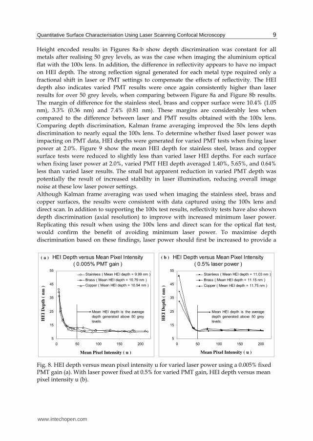
Height encoded results in Figures 8a-b show depth discrimination was constant for all

metals after realising 50 grey levels, as was the case when imaging the aluminium optical

flat with the 100x lens. In addition, the difference in reflectivity appears to have no impact

on HEI depth. The strong reflection signal generated for each metal type required only a

fractional shift in laser or PMT settings to compensate the effects of reflectivity. The HEI

depth also indicates varied PMT results were once again consistently higher than laser

results for over 50 grey levels, when comparing between Figure 8a and Figure 8b results.

The margin of difference for the stainless steel, brass and copper surface were 10.4% (1.05

nm), 3.3% (0.36 nm) and 7.4% (0.81 nm). These margins are considerably less when

compared to the difference between laser and PMT results obtained with the 100x lens.

Comparing depth discrimination, Kalman frame averaging improved the 50x lens depth

discrimination to nearly equal the 100x lens. To determine whether fixed laser power was

impacting on PMT data, HEI depths were generated for varied PMT tests when fixing laser

power at 2.0%. Figure 9 show the mean HEI depth for stainless steel, brass and copper

surface tests were reduced to slightly less than varied laser HEI depths. For each surface

when fixing laser power at 2.0%, varied PMT HEI depth averaged 1.40%, 5.65%, and 0.64%

less than varied laser results. The small but apparent reduction in varied PMT depth was

potentially the result of increased stability in laser illumination, reducing overall image

noise at these low laser power settings.

Although Kalman frame averaging was used when imaging the stainless steel, brass and

copper surfaces, the results were consistent with data captured using the 100x lens and

direct scan. In addition to supporting the 100x test results, reflectivity tests have also shown

depth discrimination (axial resolution) to improve with increased minimum laser power.

Replicating this result when using the 100x lens and direct scan for the optical flat test,

would confirm the benefit of avoiding minimum laser power. To maximise depth

discrimination based on these findings, laser power should first be increased to provide a


( 0.005% PMT gain )

5

15

25

35

45

55

0 50 100 150 200


HE

I D

ep

th (

nm

)

Stainless ( Mean HEI depth = 9.99 nm )

Brass ( Mean HEI depth = 10.79 nm )

Copper ( Mean HEI depth = 10.94 nm )



levels.HE

I D

epth

( n

m )


( a ) HEI Depth versus Mean Pixel Intensity


5

15

25

35

45

55

0 50 100 150 200


HE

I D

ep

th (

nm

)






levels.HE

I D

epth

( n

m )


( b )

Fig. 8. HEI depth versus mean pixel intensity u for varied laser power using a 0.005% fixed PMT gain (a). With laser power fixed at 0.5% for varied PMT gain, HEI depth versus mean pixel intensity u (b).

www.intechopen.com


10



5

15

25

35

45

55

0 50 100 150 200


HE

I D

epth

( n

m )




Mean HEI depth is the average depth

generated above 50 grey levels.

HE

I D

epth

( n

m )


Fig. 9. HEI depth versus mean pixel intensity u for varied PMT gain using a 2.0% fixed laser power.

minimum of 50 grey levels with PMT gain fixed at 0.005%. Fine tuning image brightness

should follow with increasing PMT gain to provide near image saturation. These

adjustments are simplified by using the SETCOL function in the LSCM LaserSharp2000

software to highlight saturated pixels red and lower pixel intensities as green during

scanning. However, difficulties striking a balance between saturation at highly reflective

regions and dark regions falling below an intensity threshold may arise for surfaces

containing multiple levels of reflectivity. To minimise dark regions that cause height

encoding error, adjusting the SETCOL threshold to 50 grey levels would provide a good

indicator during image acquisition while also highlighting the problem regions green prior

to image processing.

For the 100x lens, several images of the optical flat were captured using Kalman 2-4 frame averaging and direct scan with the 500 Hz scan rate. The generated HEI depths in Figure 10a show Kalman 2 provided the most benefit, reducing HEI depth 38.66% in comparison to direct scan with Kalman 3 and 4 reducing HEI depth a further 6.72% and 0.46%. When comparing direct scan results in Figure 10a with previous depth discrimination results, the 100x lens delivered significantly greater depth discrimination in the previous tests. The loss of depth discrimination was caused by a failing laser power supply during Kalman tests. Although depth discrimination improved with frame averaging, no benefit to lateral resolution was achieved when imaging the 0.25 µm metal graticules at Nyquist zoom. Figure 10b presents the average contrast measured across the MBI of graticule structures captured using direct scan and Kalman 2-4 frame averages. Vertical contrast across horizontal graticules on average measured higher than horizontal contrast. The cause of this asymmetric contrast was in scan rate tests associated with continuous scanning in the x direction. In addition to limited improvements for lateral resolution, Kalman averaging becomes impractical for even the 500-750 Hz when imaging large 3D series due again to increased acquisition time.

www.intechopen.com


11

HEI Depth versus Kalman Frame

Averaging

Direct

Scan

Kal 3 (

45.3

8%

)

Kal 2 (

38.6

6%

)

Kal 4 (

45.8

4%

)

5

15

25

35

0 1 2 3 4

Kalman Frame Averages ( 1 - 4 )

HE

I D

ep

th (

nm

)

Kal 2 reduced

depth 38.66%

Contrast versus Kalman Frame

Averaging ( 0.25 um graticule )

Direct

Scan

Kal 3

Kal 2

Kal 4

30%

40%

50%

60%

70%

0 1 2 3 4

Kalman Frame Averages ( 1 - 4 )

Co

ntr

ast (%

)

Horizontal Graticules ( Vertical Contrast )

Vertical Graticules ( Horizontal Contrast )

HE

I D

epth

( n

m )

Kalman Frame Averages ( 1-4 )

( a )

Co

ntr

ast

( %

)

Kalman Frame Averages ( 1-4 )

( b )

Fig. 10. HEI depth indicates frame averages improved depth discrimination (a) while no benefit to lateral resolution was gained with contrast remaining steady (b).

Confocal Aperture Settings

The impact of the confocal aperture settings on both depth discrimination and lateral resolution were also assessed using the aluminium optical flat and chromium structures on the Richardson slide. Since the confocal aperture is a critical parameter in maximising LSCM resolutions, varied aperture tests measured lateral contrast and measured HEI depth for the 10x, 20x, 50x and 100x objective lenses. Images of the optical flat were captured with each lens using zoom 999 for a 0.7, 1.0, 1.2, 1.7, 2.7 and 3.7 mm aperture setting. Height encoding generated the averaged HEI depth versus aperture size in Figure 11. On assessment, HEI

HEI Depth versus Confocal Aperture

( 10x, 20x, 50x & 100x lenses )

0.7

mm

1.0

mm

1.2

mm

1.7

mm

2.7

mm

3.7

mm

5

30

55

0.5 1 1.5 2 2.5 3 3.5 4

Confocal Aperture ( mm )

HE

I D

epth

( n

m )

10x Lens 20x Lens 50x Lens 100x Lens

HE

I D

epth

( n

m )


( a )

Fig. 11. The Influence of confocal aperture setting on depth discrimination for the 10x, 20x, 50x and 100x lenses.

www.intechopen.com


12

Contrast versus Confocal Aperture

3.7

mm1

.2m

m

1.7

mm

0.7

mm

10%

20%

30%

40%

50%

60%

70%

0.5 1.5 2.5 3.5


Co

ntr

ast (%

)

10x ( 1.0 um resolution bars)

20x ( 0.5 um graticules )

Contrast versus Confocal Aperture

3.7

mm

1.7

mm

1.2

mm

0.7

mm

10%

20%

30%

40%

50%

60%

70%

0.5 1.5 2.5 3.5


Co

ntr

ast (%

)



Co

ntr

ast

( %

)


( a )

Co

ntr

ast

( %

)


( b )

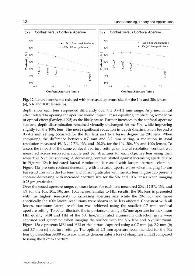
Fig. 12. Lateral contrast is reduced with increased aperture size for the 10x and 20x lenses (a), 50x and 100x lenses (b).

depth show each lens responded differently over the 0.7-1.2 mm range. Any mechanical

effect related to opening the aperture would impact lenses equalling, implicating some form

of optical effect (Pawley, 1995) as the likely cause. Further increases in the confocal aperture

size and depth discrimination remained virtually unchanged for the 50x, while improving

slightly for the 100x lens. The most significant reduction in depth discrimination beyond a

0.7-1.2 mm setting occurred for the 10x lens and to a lesser degree the 20x lens. When

comparing the difference between 0.7 mm and 3.7 mm setting, a reduction in axial

resolution measured 49.1%, 42.7%, 13% and -20.2% for the 10x, 20x, 50x and 100x lenses. To

assess the impact of the same confocal aperture settings on lateral resolution, contrast was

measured across resolved graticule and bar structures for each objective lens using their

respective Nyquist zooming. A decreasing contrast plotted against increasing aperture size

in Figures 12a-b indicated lateral resolution decreased with larger aperture selections.

Figure 12a presents contrast decreasing with increased aperture size when imaging 1.0 µm

bar structures with the 10x lens, and 0.5 µm graticules with the 20x lens. Figure 12b presents

contrast decreasing with increased aperture size for the 50x and 100x lenses when imaging

0.25 µm graticules.

Over the tested aperture range, contrast losses for each lens measured 20%, 12.5%, 13% and

4% for the 10x, 20x, 50x and 100x lenses. Similar to HEI results, the 10x lens is presented

with the highest sensitivity to increasing aperture size while the 20x, 50x and more

specifically the 100x lateral resolutions were shown to be less affected. Consistent with all

lenses, maximum lateral resolution was achieved using the smallest 0.7 mm confocal

aperture setting. To better illustrate the importance of using a 0.7mm aperture for maximum

HEI quality, MBI and HEI of the 600 line/mm ruled aluminium diffraction grate were

captured and generated when imaging the surface with the 50x lens and Nyquist zoom.

Figure 13a-c presents MBI and HEI of the surface captured using a 0.7 mm (a), 2.2 mm (b)

and 3.7 mm (c) aperture settings. The optimal 2.2 mm aperture recommended for the 50x

lens by LaserSharp2000 software, already demonstrates a loss of sharpness in HEI compared

to using the 0.7mm aperture.

www.intechopen.com


13

Fig. 13. Both HEI and MBI of the 600 line/mm ruled diffraction grate captured with a 0.7 mm (a), 2.2 mm (b) and 3.7 mm confocal aperture size.

Axial Resolution Tests

The Radiance2000 LSCM axial resolutions were measured from the through focal plane intensity distributions, applying the full width half maximum (FWHM) approximation often used by microscopist (Pawley, 1995; Webb, 1996). Performing xz scans of the optical flat for each objective lens with Nyquist zoom, through focal pixel intensities were then extracted and plotted against the z displacement of the microscope stage in Figure 14a using a 50 nm step size. Indicated on each intensity distribution are the measured FWHM approximations for the 10x, 20x, 50x and 100x lenses. Figure 14b illustrates the through focal xz scan captured with the 100x lens and the relationship of the intensity distribution to z displacement. Comparing measured and theoretical FWHM axial resolutions summarised in Table 1, measured axial resolutions were between 18-68% worse than FWHM Plane axial resolutions calculated for imaging a plane reflective surface by (Xiao and Kino, 1987). It is well documented in literature that LSCM axial resolution is far greater when applying image processing techniques to extract height maps from the raw 3D image series. Throughout LSCM performance testing, HEI depth was calculated using the centre of mass image (CM) processing algorithm that delivered depth discrimination (axial resolution) many times higher than the measured or theoretical FWHM resolutions presented in Table 1. A measure of HEI axial resolution using the centre of mass technique was gained when performing earlier confocal aperture tests for the 10x, 20x, 50x and 100x lenses. In Figure 15, the same HEI depths generated for a 0.7 mm aperture setting highlights the difference in axial resolution for each objective lens NA. For comparison, reprocessing the images generated HEI axial resolutions in Figure 15 associated with the peak detection (PD) and the powers height encoding techniques. The peak detection algorithm determines surface height from the axial position containing the

(a) 0.7 mm Aperture

MBI

HEI

(b) 2.2 mm Aperture

HEI

(c) 3.7 mm Aperture

HEI

MBI MBI

www.intechopen.com


14

Intensity versus Axial Displacement

( 10x, 20x, 50x & 100x lenses axial FWHM )

10x20x50x100x

FWHM

0

50

100

150

200

250

0 5 10 15 20 25 30 35

Axial Displacement (um)

Pix

el In

tensity ( G

rey level

Pix

el I

nte

nsi

ty (

Gre

y l

evel

s )

Axial Displacement ( µm )

( a ) Extracted axial

intensity distribution

( z ) Displacement

( b )

Fig. 14. Axial FWHM resolution approximations for the 10x, 20x, 50x and 100x lenses (a) and the typical axial intensity distribution extracted from a through focal plane xz scan with the 100x lens (b).

Objective Lens

NA

MeasuredFWHM

FWHM Plane (Xiao and Kino, 1987)

Difference in Measured From Theory

LU Plan 10x 0.30 8.02 µm 4.77 µm 68.1% more




Table 1. Measured FWHM axial resolutions and theoretical FWHM differences.

HEI Depth versus Numerical Aperture

( 10x, 20x, 50x & 100x lenses )

10x 0.046 μm

10x 0.068 μm

10x 1.340 μm

0.0

0.1

0.2

0.3

0.1 0.2 0.3 0.4 0.5 0.6 0.7 0.8 0.9

Lens Numerical Aperture ( NA )

HE

I D

epth

( μ

m )

-0.1

0.1

0.3

0.5

0.7

0.9

1.1

1.3

1.5

1.7Center of Mass (CM)

Power 2

Peak Detection (PD)

0.45

NA

0.3

NA

0.8

NA

0.9

NAHE

I D

epth

( µ

m )

Lens Numerical Aperture ( NA )

Fig. 15. Axial resolutions achieved in HEI using the centre of mass, powers and peak detection algorithms versus objective lens numerical aperture NA.

www.intechopen.com


15

brightest pixel within the through focal plane intensity distribution (Sheppard and Matthews, 1987; Sheppard and Shotton 1997; Pawley 1995; Jordan et al., 1998). For the powers technique, through focal intensities are raised to the 2nd power before calculating the centre of mass surface position. Further increases in the power used and HEI depth approach those generated by peak detection as the weighting on brighter pixels increases. Performing xz scans for the FWHM axial resolution approximations or capturing xyz series for generating HEI depths both involved using a 50-100 nm step size. Oversampling with finer steps ideally passes all xy surface points through the focal plane central region. Figure 16 illustrates a through focal intensity distribution for the 100x lens captured using a 50 nm step size. The peak intensity on the 50 nm stepped distribution coincides with a surface point passing through or near the focal plane central region. The two solid profile lines in Figure 16 illustrate when using a 0.5 µm step size, the surface may not pass through the ideal central region but rather above or below the central position. The location of the CM surface position using a 50 nm step size was 3.176 µm. The difference between CM surface positions generated for the two 0.5 µm stepped profiles is 0.06813 µm, which can vary depending on how the surface aligns with the focal plane. For peak detection identified by PD in Figure 16, the surface positions for the same 0.5 µm stepped profiles varied a much greater 0.3 µm. Table 2 summarises the centre of mass HEI depths, measured FWHM and theoretical FWHM axial resolutions. Also listed in Table 2 are the factors of improvement for HEI axial resolution over measured and theoretical values. To assess the impact of step size on HEI depth and subsequent HEI axial resolutions, images of the optical flat were captured using oversampled to near Nyquist step size. Based on measured FWHM axial resolutions in Table 1 the approximate Nyquist step sizes for the 10x, 20x, 50x and 100x lenses are summarised in Table 3. Also summarised in Table 3 are the tested step sizes (1-3) in microns and as percentages of the approximated Nyquist steps. On capturing images for the tested step sizes using zoom 999 and the 500Hz scan rate, height encoding the images generated the HEI depth versus the percentage of Nyquist steps in Figure 17.

Undersampling Through Focus

( 100x lens intensity distribution )

0

50

100

150

200

250

2 2.5 3 3.5 4 4.5

Axial Displacement ( μm )

Pix

el In

tensity ( G

rey level

50 nm Step size

0.5 μm Step size( 0.5 μm steps )

CM difference 0.06813 μm

PD difference 0.30 μm

( 0.5 μm steps )

CM position 3.176 μm

( 50 nm steps )

Axial Displacement ( µm )

Pix

el I

nte

nsi

ty (

Gre

y l

evel

s )

Fig. 16. Difference in accuracy between peak detection & centre of mass height encoding.

www.intechopen.com


16

Factor HEI Depth Improved on Objective Lens NA

Centre of MassHEI Depth

MeasuredFWHM

TheoreticalFWHM Measured FWHM Theoretical FWHM

0.30 44.4 nm 8.02 µm 4.77 µm ≈ 181 x ≈ 107 x

0.45 18.2 nm 2.50 µm 2.12 µm ≈ 137 x ≈ 116 x

0.80 12.4 nm 0.90 µm 0.55 µm ≈ 73 x ≈ 44 x

0.90 10.8 nm 0.47 µm 0.39 µm ≈ 44 x ≈ 36 x

Table 2. Comparison of measured and theoretical FWHM axial resolutions to HEI depths generated by the centre of mass height encoding algorithm.

Objective Lens NA

NyquistStep size

Test step size (1) % of Nyquist Step

Size


Size


Size

0.30 3.48 µm 0.10 µm (≈ 3%) 1.80 µm (≈ 52%) 3.60 µm (≈ 103%)

0.45 1.09 µm 0.05 µm (≈ 5%) 0.50 µm (≈ 46%) 1.00 µm (≈ 92%)

0.80 0.39 µm 0.05 µm (≈ 13%) 0.25 µm (≈ 64%) 0.50 µm (≈ 128%)

0.90 0.20 µm 0.05 µm (≈ 25%) 0.15 µm (≈ 75%) 0.30 µm (≈ 147%)

Table 3. Summary of tested step sizes for the 10x, 20x, 50x and 100x lens as percentages of Nyquist step size.

HEI Depth versus Percentage of Nyquist Step Size

( 10x, 20x, 50x & 100x lenses )

0.00

0.05

0.10

0.15

0.20

0.25

0.30

0.35

0.40

0% 20% 40% 60% 80% 100% 120% 140% 160%

Fraction of Nyquist Step Size

HE

I D

epth

( um

)

10x Lens 20x Lens 50x Lens 100x Lens

HE

I D

epth

( µ

m )

Percentage of Nyquist Step Size ( % )

Fig. 17. HEI depth versus percentage of Nyquist step size for the 10x, 20x, 50x & 100x lenses.

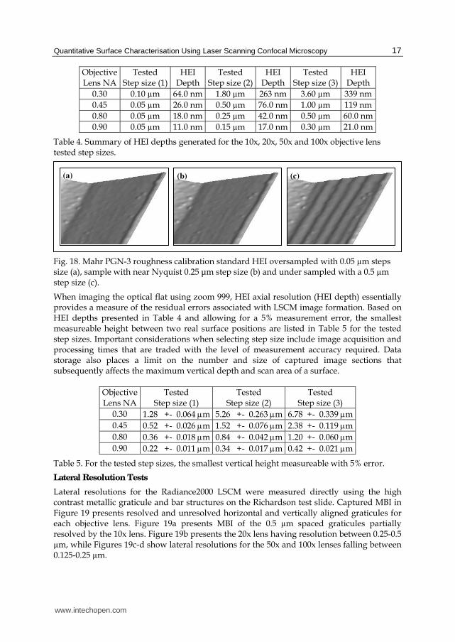
Presented in Figure 17 and summarised in Table 4, tests show a marked increase in HEI depth and therefore reduced axial resolution when increasing step size to near Nyquist values. An insufficient sampling rate becomes obvious when attempting to image sloping surfaces. Figure 18a-c presents HEI of the silica Mahr PGN-3 roughness calibration standard captured with the 100x lens using 0.05 µm (a), 0.25 µm (b) and 0.5 µm step size (c). The Nyquist step size for the 100x lens is approximately 0.20 µm and using 0.25 µm steps in Figure 18b already show signs of missing surface information with Figure 18c clearly under sampled with 0.5 µm step size.

www.intechopen.com


17

ObjectiveLens NA

Tested Step size (1)

HEI Depth


HEI Depth


HEI Depth

0.30 0.10 µm 64.0 nm 1.80 µm 263 nm 3.60 µm 339 nm

0.45 0.05 µm 26.0 nm 0.50 µm 76.0 nm 1.00 µm 119 nm

0.80 0.05 µm 18.0 nm 0.25 µm 42.0 nm 0.50 µm 60.0 nm

0.90 0.05 µm 11.0 nm 0.15 µm 17.0 nm 0.30 µm 21.0 nm

Table 4. Summary of HEI depths generated for the 10x, 20x, 50x and 100x objective lens tested step sizes.

Fig. 18. Mahr PGN-3 roughness calibration standard HEI oversampled with 0.05 µm steps size (a), sample with near Nyquist 0.25 ┤m step size (b) and under sampled with a 0.5 µm step size (c).

When imaging the optical flat using zoom 999, HEI axial resolution (HEI depth) essentially provides a measure of the residual errors associated with LSCM image formation. Based on HEI depths presented in Table 4 and allowing for a 5% measurement error, the smallest measureable height between two real surface positions are listed in Table 5 for the tested step sizes. Important considerations when selecting step size include image acquisition and processing times that are traded with the level of measurement accuracy required. Data storage also places a limit on the number and size of captured image sections that subsequently affects the maximum vertical depth and scan area of a surface.

ObjectiveLens NA




0.30 1.28 +- 0.064 μm 5.26 +- 0.263 μm 6.78 +- 0.339 μm

0.45 0.52 +- 0.026 μm 1.52 +- 0.076 μm 2.38 +- 0.119 μm

0.80 0.36 +- 0.018 μm 0.84 +- 0.042 μm 1.20 +- 0.060 μm

0.90 0.22 +- 0.011 μm 0.34 +- 0.017 μm 0.42 +- 0.021 μm

Table 5. For the tested step sizes, the smallest vertical height measureable with 5% error.

Lateral Resolution Tests

Lateral resolutions for the Radiance2000 LSCM were measured directly using the high contrast metallic graticule and bar structures on the Richardson test slide. Captured MBI in Figure 19 presents resolved and unresolved horizontal and vertically aligned graticules for each objective lens. Figure 19a presents MBI of the 0.5 µm spaced graticules partially resolved by the 10x lens. Figure 19b presents the 20x lens having resolution between 0.25-0.5 µm, while Figures 19c-d show lateral resolutions for the 50x and 100x lenses falling between 0.125-0.25 µm.

(a) (b) (c)

www.intechopen.com


18

1.0μm 0.5μm 0.5μm 0.25μm 0.25μm 0.125μm 0.25μm 0.125μm

( b ) 20x ( d ) 100x ( c ) 50x( a ) 10x

Horizontal

Vertical

Fig. 19. Upper and lower binding limits for the 10x, 20x, 50x and 100x objective lens lateral resolution.

Contrast measured from MBI of the test structures were plotted against line spacing in

Figure 20 for each lens. Also contained in Figure 20 are theoretical FWHM lateral resolutions

at 33.3% contrast, corresponding to a FWHM separation distance predicted by (Brakenhoff,

et al., 1979). Contrasts measured for the 20x, 50x and 100x lenses were limited by the

degraded state of the finer bar structures found on the Richardson slide. Therefore the 0.125

µm graticules unresolved by the 50x and 100x lenses, and the 0.25 µm graticules unresolved

Contrast versus Graticule Line Spacing

( 10x, 20x, 50x & 100x lenses )

0.50

1.00

0.80

1.50

2.0

0

0.50.25

0.25

0.0

0.1

0.2

0.3

0.4

0.5

0.6

0.7

0.8

0.9

1.0

1.1

1.2

0.0 0.2 0.4 0.6 0.8 1.0 1.2 1.4 1.6 1.8 2.0

Line Spacing ( µm )

Contrast ( %

)

10x Lens 20x Lens

50x Lens 100x Lens

Theoretical contrast 33.33%

( Brakenhoff, et al., 1979 ) 0.239 μm 0.477 μm

0.268 μm 0.716 μm

Co

ntr

ast

( %

)

Graticule Line Spacing ( µm )

Fig. 20. Measured contrast versus graticule line spacing µm for the 10x, 20x, 50x, &100x lenses.

www.intechopen.com


19

Objective Lens

NA

Measured FWHM or Limits

FWHM (Brakenhoff et al., 1979)

Difference in Measured From Theory


LU Plan 20x 0.45 0.43 µm 0.477 µm 9.8% less



Table 6. Measured FWHM lateral resolutions, binding limits & theoretical FWHM.

by the 20x lens in Figure 19 were used to approximate zero contrast for these lenses in Figure 20. Interpolating a 33.3% contrast between 0.5-0.8 µm for the 10x, 0.25-0.5 µm for the 20x, and 0.125-0.25 µm for the 50x and 100x lenses estimated measured FWHM resolutions to be approximately 0.77, 0.43, 0.22 and 0.19 µm. It should be noted measured FWHM resolutions for the 20x, 50x and 100x lenses are slightly better than would usually be due to setting the resolution limit for these lenses at 0.125 µm or 0.25 µm, when in fact zero contrast will measure in at possibly higher line spacing. However, FWHM resolutions measured from plots in Figure 20 provide a fair comparison to FWHM calculated from theory (Brakenhoff et al., 1979). Table 6 summaries theoretical FWHM lateral resolutions, measured FWHM lateral resolutions and the percentile of difference for each objective lens. In the LSCM reflection imaging mode, optical effects caused by discontinuous surface edges have significant influence on the formation of height encoded images. Light reflected from the edges of a surface relief constructively and destructively interfere (Juskaitis and Wilson, 1992), modifying the through focal plane intensity distribution. Both the centre of mass and peak detection height encoding algorithms break down in locating the surface position accurately in these regions. The centre of mass algorithm tends to over or undershoot the real surface position across such structures. To determine the limits of HEI lateral resolution for each objective lens based on limitations set by HEI artefact, images of a straight edge found on the Richardson slide were captured using twice Nyquist zoom and the 50 nm step sizes. Figure 21 present HEI of the edge structure captured with each objective lens to illustrate the lateral xy width (wavelength) of the image artefact unique to the 10x (a), 20x (b), 50x (c) and 100x (d) lenses. The artefact measured approximately 4.02 µm (a), 2.87 µm (b), 1.47 µm (c) and 1.14 µm (d) for the respective lens. Filter applications in TrueMap V4 image processing software established shortwave (┣s) cut-offs limits of approximately 13.5 µm, 7 µm, 3.5 µm and 2.7 µm that completely removed the artefact from images prior to quantitative surface analysis.

Image Acquisition of Various Samples using Optimal Settings

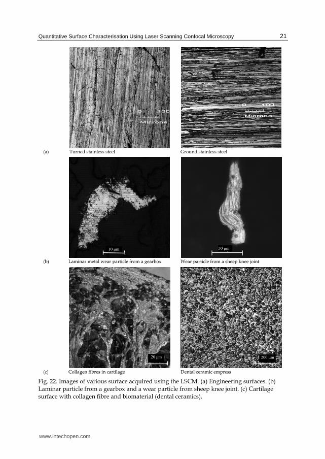
Based on the LSCM resolution tests and assessment rules in the 4288 ISO standard for quantitative surface characterisation, it has been concluded that the confocal system can be used to measure surface roughness over a range of 0.05 microns to a few microns (Peng & Tomovich, 2008). The above studies on the Radiance2000 confocal microscope system performance and hardware settings have provided a guide to selecting the appropriate objective lens and system setting for quantitative surface characterisation. Images of engineering and biomaterial surfaces, metallic wear debris and collagen structures of cartilage samples extracted from sheep knee joints are shown in Figure 22 to demonstrate the capability of LSCM for various applications. To acquire the images shown in Figure 22, different sample preparation methods were used. For the scanning of engineering surfaces shown in Figure 22a and biomaterial surface (dental ceramic) in Figure 22c right, the surfaces were cleaned and scanned directly. The

www.intechopen.com


20

( a ) 10x Lens ( b ) 20x Lens

( c ) 50x Lens ( d ) 100x Lens

≈ 1.47 μm

≈ 4.02 μm ≈ 2.87 μm

≈ 1.14 μm

Fig. 21. HEI of the edge structure captured with each objective lens to illustrate the lateral xy width (wavelength) of the image artefact.

same method was applied when acquiring the metallic wear particle image shown in Figure 22b left. For the cartilage wear particle shown in Figure 22b right and cartilage surface in Figure 22c left, these samples required staining before imaging. The wear particle generated in a sheep’s knee was collected from synovial fluid encapsulated within the knee joint. The extracted fluid was mixed with glutaraldehyde, agitated to mix the fluids and then stored in a refrigerator set at approximately 4 degrees Celsius for more than 24 hours. This process enabled the fixing of particles to prevent any further deterioration from occurring. Wear particles were then dyed and fixed onto glass slides for imaging. The cartilage image shown in Figure 22c left was acquired using the fluorescence imaging mode after the sample was stained via immunohistochemical (IHC) staining methods.

3.2 Image processing Image processing is a three-step process before quantitative image analysis is performed using the developed system. The three steps are: (a) 3D image construction; (b) elimination of image distortion and artefacts; and (c) image stitching. Before performing quantitative image analysis, a series of 2D images needs to be compiled into HEI format so that height information can be obtained for surface characterisation in 3D. Thus, HEI construction is the first step in the procedures used for image processing. Similar to other image acquisition systems, noise and distortion often associated with LSCM images are then reduced or eliminated with follow up HEI processing techniques. Finally, the stitching together of multiple HEI is a necessary step to form a large surface mosaic for

www.intechopen.com


21

(a) Turned stainless steel Ground stainless steel

(b) Laminar metal wear particle from a gearbox Wear particle from a sheep knee joint

10 μm 50 μm

20 μm 200 μm

(c) Collagen fibres in cartilage Dental ceramic empress

Fig. 22. Images of various surface acquired using the LSCM. (a) Engineering surfaces. (b) Laminar particle from a gearbox and a wear particle from sheep knee joint. (c) Cartilage surface with collagen fibre and biomaterial (dental ceramics).

www.intechopen.com


22

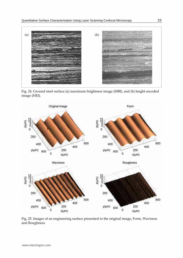
ISO compliant measurements. so a large surface is generated for ISO compliant measurements. The details for the three phases of image processing are presented in as follows. A series of 2D images is firstly obtained using the LSCM. To perform 3D surface characterisation, 3D information first needs to be extracted from the 2D image series. To construct 3D surface maps from raw LSCM data, a number of height encoding algorithms have been tested and evaluated. The tests also served to provide HEI cut off limits for developing a HEI reconstruction technique that removes sub resolution information such as edge artefact using wavelet filtering. Three surface detection algorithms including peak detection, centre of mass and centre of mass to a power have been tested for accuracy in locating the real surface. The established process can create the appropriate 3D images for surface characterisation. The procedures for image reconstruction can be found in Figure 23. Figure 24 shows a maximum brightness and height encoded image of an engineering surface complied from a set of 2D images acquired using the LSCM. The second step in 3D image construction is to apply filters to separate surface form, waviness and roughness information for surface measurement. This step is necessary to analyse specific and meaningful surface information in different wave length for specific purposes. In this project, we have used the wavelet method to filter and separate original surface data into long, medium and short wave length, which corresponds to form, waviness and roughness information. Figures 25 and 26 show examples of the process conducted on an engineering surface and the surface of a metallic wear particle.

Fig. 23. Image reconstruction procedures using the centre of mass algorithm.

Load 3D volume data of a surface

Read intensity data from each pixel in z column

Store centre of mass intensity in MBI

Assign grey level to the centre of mass location

and display in HEI

Search for the centre of mass

Store image files for quantitative analysis

www.intechopen.com


23

Fig. 24. Ground steel surface (a) maximum brightness image (MBI), and (b) height encoded image (HEI).

Fig. 25. Images of an engineering surface presented in the original image, Form, Waviness and Roughness.

(a) (b)

www.intechopen.com


24

Fig. 26. Separated Form, Waviness and Roughness of a particle image.

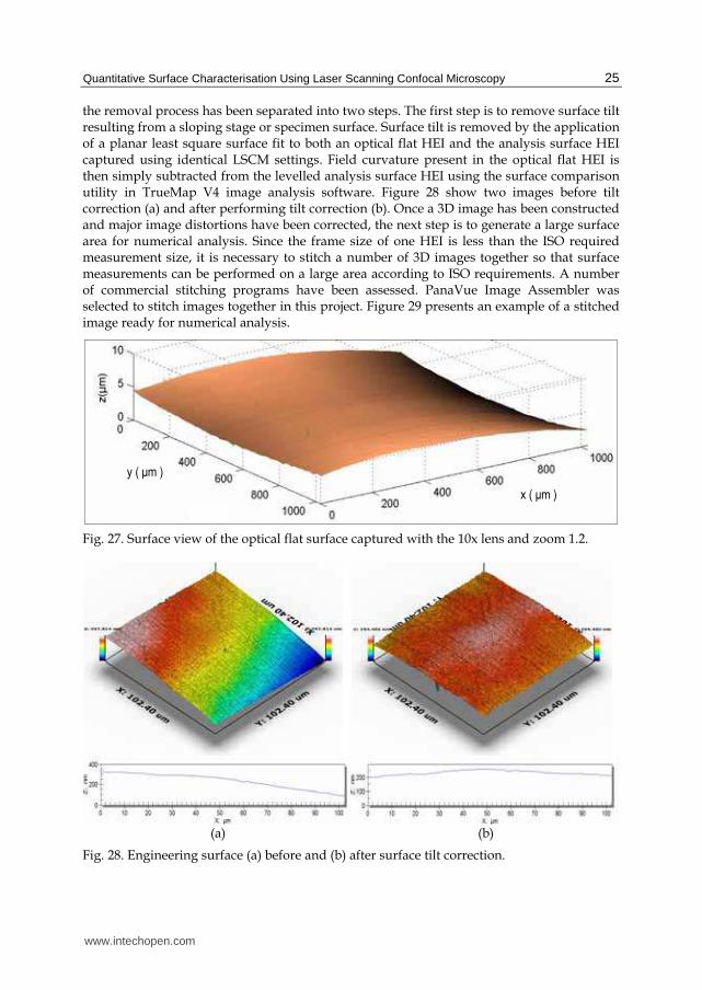
Similar to any other imaging systems, image distortion exists and has to be eliminated to ensure the accuracy of surface measurements. A series of tests have been conducted to evaluate system related image distortions which may exist in generated 3D images. It has been found that objective lens field curvature and surface tilt are the two main issues affecting surface characterisation to be conducted later. Field curvature is a lens aberration that introduces distortion to most existing optical microscopy application. Although the 10x, 20x, 50x and 100x LU Plan objective lenses used in this project are all corrected for field curvature, noticeable curvature in HEI still remains when imaging with low zoom settings. Figure 27 present an example 3D height encoded surface view of the optical flat, imaged with the 10x lens using zoom 1.2. The z axis has been rescaled to accentuate the effects of field curvature on distorting what should be a flat surface. The presence of surface tilt, field curvature and scanning system distortions all contribute to the total form error present in HEI. The application of least square curve fitting is one potential solution to removing field curvature and scanning distortion prior to more accurate industrial surfaces analysis. Another potential solution is to simply subtract known distortions obtained with the optical flat prior to industrial surface analysis. In our study,

www.intechopen.com


25

the removal process has been separated into two steps. The first step is to remove surface tilt resulting from a sloping stage or specimen surface. Surface tilt is removed by the application of a planar least square surface fit to both an optical flat HEI and the analysis surface HEI captured using identical LSCM settings. Field curvature present in the optical flat HEI is then simply subtracted from the levelled analysis surface HEI using the surface comparison utility in TrueMap V4 image analysis software. Figure 28 show two images before tilt correction (a) and after performing tilt correction (b). Once a 3D image has been constructed and major image distortions have been corrected, the next step is to generate a large surface area for numerical analysis. Since the frame size of one HEI is less than the ISO required measurement size, it is necessary to stitch a number of 3D images together so that surface measurements can be performed on a large area according to ISO requirements. A number of commercial stitching programs have been assessed. PanaVue Image Assembler was selected to stitch images together in this project. Figure 29 presents an example of a stitched image ready for numerical analysis.

x ( μm )

y ( μm )

Fig. 27. Surface view of the optical flat surface captured with the 10x lens and zoom 1.2.

(a) (b)

Fig. 28. Engineering surface (a) before and (b) after surface tilt correction.

www.intechopen.com


26

Fig. 29. Stitched image after cross-correlation and blending for numerical analysis.

3.3 Quantitative image analysis Quantitative image analysis involves using a set of numerical parameters to characterise surface morphology for various purposes. There are in general two sets of numerical parameters for surface characterisation. They are field parameters and feature parameters (Jiang et al., 2007; Scott, 2009). Field parameters are often used to classify averages, deviations, extremes and specific features on a scale-limited continuous surface (Jiang et al., 2007). Surface roughness (Sa and Sq), skewness, kurtosis and spectral analysis are normally used as field parameters to describe how rough or smooth a surface is along with texture distribution. These parameters, also called profile surface texture parameters, have been commonly and traditionally used in many applications. Feature parameters characterise surface features and their relationship for functional diagnostics and prediction (Scott, 2009). The feature parameters are relatively new and have not been widely used for surface characterisation. For this reason, only common field parameters have been used in our study. In particular, the surface roughness parameter Sa is used to evaluate the performance of the above developed image acquisition, processing and analysis techniques. A set of manufactured nickel specimens certified for various roughness specifications, and a front coated aluminium optical flat were used to test the above developments. These samples have a well defined surface structure and differences in surface roughness. The three selected nickel surfaces have average roughness values of 0.05 µm (ground surface), 1.60 µm and 3.20 µm respectively (vertically milled surface). The smooth front coated aluminium optical flat has a surface roughness of less than 5 nm. This sample was used to test the limits of the LSCM imaging system and approximate system measurement error. The surfaces were imaged using the system established in the section above. Image

www.intechopen.com


27

reconstruction, filtering and stitching processes were conducted as described. Table 7 presents the analysis results prior to corrective image processing, post corrective image processing and the associated percentile of improvement for Sa.

Sample (Sa)

Average Sa before correction

(µm)

Average Sa after correction (µm)

Average Sa for stitched image

(µm)

Percentage Sa being corrected

(%)

0.005µm Optical Flat

0.114 0.009 0.009 92

0.05µm Ground Surface

0.591 0.054 0.054 91

1.60µm Milled Surface

1.511 1.516 1.624 7.5


4.100 3.059 3.200 22

Table 7. Average Sa for the tested samples before and after corrective image processing, and on stitching surface mosaics.

Prior to corrective imagine processing, the Sa values generated for raw images obtained with the LSCM did not match the reference values certified by the manufacturer. On processing images in TrueMap V4 to eliminate field curvature and surface tilt, Sa values for the corrected images matched or were closer to the manufacturer specified Sa values. In Table 7, the percentage Sa values were corrected by are calculated as follow:

_ _

_

%abefore correction aafter correction

acorrectedabefore correction

S SS

S

−=

Thereafter, the corrected images were stitched together forming a large image. Table 8 show the accuracy of Sa before and after the correction and stitching processes, highlighting the improvement in Sa measurements. This demonstrates that more accurate and precise topographical surface data has been extracted from large images.

Sample Relative Error* of Sa before correction (%)

Relative Error* of Sa after correction and before

stitching (%)

Accuracy of Sa after correction

and stitching (%)

0.005µm Optical Flat

>100 80 20

0.05µm Ground Surface

>100 8 92


5.56 1.5 98.5


28.13 0.01 99.99

* The error is calculated as % 100%a a

a

measuredS value true S value

true S value

−= ×

Table 8. The accuracy of Sa for test samples before and after corrective image processing, and on stitching surface mosaics.

www.intechopen.com


28

4. Discussion

This project has clearly demonstrated that laser scanning confocal microscopy can be used for quantitative surface measurements. The technique is suited to acquiring surface roughness information within the range of approximately 0.05 microns to a few microns with reasonably high accuracy. This allows the use of the system for surface characterisation on a wide range of surfaces, particularly engineering surfaces and wear particles. The study has also examined optimal system settings and objective lens for quantitative surface characterisation. Although there is literature on the effects of LSCM settings in relation to image quality, this project has, for the first time, systematically investigated the issues associated with the measurement of engineering surfaces. From this study the recommended settings for scan rate, laser power, PMT gain, confocal aperture setting and step size provide the Radiance2000 LSCM user with a clear guide to obtaining images of suitable quality for quantitative analysis. The study has also identified the effects of field curvature and surface tilt on subsequent measurements, when selecting the appropriate objective lens and zoom to meet ISO evaluation area requirements. The results confirm that the removal of these distortions and artefacts during image reconstruction are important steps to ensuring images contain accurate surface information. Techniques have been tested, evaluated and selected for the removal of surface tilt and field curvature during 3D image reconstruction. However, artefact associated with the formation of HEI at edge structures require further assessment of appropriate techniques needed to minimise this effect and remove the residual artefact during image reconstruction. Part of this project was to research suitable image stitching algorithms. Due to the small field of view in confocal imaging, the stitching of multiple images into a large surface mosaic was a necessary procedure developed for performing measurements that satisfy ISO area of assessment rules. The project used a range of samples with different surface roughness to evaluate the above

developments. The results have shown the developed technique cannot accurately quantify

the roughness of the very smooth optical flat, having a surface roughness of less than 5 nm.

This was highlighted by the large error associated with the optical flat roughness

measurement. The developed technique was able to measure surface roughness down to

0.05 microns with an accuracy of 90%. Based on measurement results obtained for the

surfaces of known roughness, we have concluded the LSCM imaging technique is suited to

measuring surfaces having roughness values ranging from 0.1 to approximately 5 microns.

This roughness range is covered by the 250-2500 µm2 assessment areas set out in the ISO

4288 measurement standards. However, further tests for surfaces having roughness values

approaching 10 micron is required to confirm the 2500 µm2 range is within practical limits of

the LSCM imaging system. Important consideration when imaging for a 2500 µm2

assessment area, include imaging time and storage space when capturing a sufficient

number of images to form a surface mosaic.

5. Conclusion

This project, based on the studies of LSCM imaging fundamentals, has developed a reliable and accurate 3D quantitative surface measurement system using laser scanning confocal microscopy. The image acquisition technique and procedures have been developed for providing images with optimal quality, resolution and that are representative of real surface information. In addition, the project has investigated image processing techniques essential

www.intechopen.com


29

for accurate surface analysis. The project has made progress in the following aspects. (a) Quantitative determination of the LSCM resolutions and its capability in 3D surface measurement applications have been carried out in this study. (b) Comprehensive image acquisition and processing techniques have been developed for numerical analysis. In particular, reconstruction of 3D height encoded surface maps have been improved, and image processing methods have been investigated for the removal of field curvature, surface tilt and image artefact such as those generated by surface edges. (c) Based on the above developments, a quantitative surface measurement system using the Radiance2000 confocal microscope has been advanced for 3D surface characterisation. The reliability and accuracy of the system have been validated with the measurement of calibration standards, industrially machined surfaces and wear particles. We hope the work will extend the usage of the laser scanning confocal technique from visual inspection to quantitative analysis in many fields.

6. References

Bennett JM and Mattsson L (1989), Introduction to Surface Roughness and Scattering, Optical Society of America, Washington DC.

Bernabeu E, Sanchez-Brea LM, Siegmann P, Martinez-Anton JC, Gomez-Pedrero JA, Wilkening G, Koenders L, Muller F, Hildebrand M and Hermann H (2001), Classification of surface structures on fine metallic wires, Applied Surface Science, Vol. 180, pp 191-199.

Brakenhoff GJ, Blom P and Barends P (1979), Confocal scanning light microscopy with high aperture immersion lenses, J. Microsc., Vol. 117, pp 219-232.

Brown JM and Newton CJ (1994), Quantified three-dimensional imaging of pitted aluminium surfaces using laser scanning confocal microscopy, British Corrosion Journal, Vol 29 No 4, pp 261-269.

Chescoe D and Goodhew PJ (1990), in Royal Microscopical Society Microscopy Handbook 20, Oxford University Press, New York.

Conroy M and Armstrong J (2005), A comparison of surface metrology techniques, Journal of Physics: Conference Series 13, pp 458-165.

DeGarmo EP, Black JT and Kohser RA (1997), Materials and Processes in Manufacture, Eighth Edition, Prentice Hall International USA, pp 289-291.

Gadelmawla ES, Koura MM, Maksoud TMA, Elewa IM and Soliman HH (2002), Roughness Parameters, Journal of Materials Processing Technology, Vol. 123, pp 133-145.

Gauldie RW, Raina G, Sharma SK and Jane JL (1994), in Atomic Force Microscopy / Scanning Tunnelling Microscopy, Edited by al. SHC e, Plenum Press, New York, pp 85-90.

Gjonnes L (1996), Quantitative Characterisation of the Surface Topography of Rolled Sheets by Laser Scanning Microscopy and Fourier Transforms, Metallurgical And Materials Transactions A, 27A, pp 2338-2346.

Hanlon DN, Todd I, Peekstok E, Rainforth WM and Van Der Zwaag S (2001), The application of laser scanning confocal microscopy to tribological research, Wear, pp 1159-1168.

Haridoss S, Shinozaki DM and Cheng PC (1990), IEEE International Symposium on Electrical Insulation, Toronto, Canada, pp 392-397.

www.intechopen.com


30

ISO standards 4288 (1996), Geometrical Product Specifications (GPS) – Surface texture: Profile method – Rules and procedures for the assessment of surface texture, ISO.

Jiang X, Scott PJ, Whitehouse DJ and Blunt L (2007), Paradigm shifts in surface metrology. Part II: The current shift, Proc. R. Soc. A, Vol. 463, pp. 2071-2099.

Jordan HJ, Wegner M and Tiziani H (1998), Highly accurate non-contact characterisation of engineering surfaces using confocal microscopy, Meas. Sci. Tecnol., UK, Vol. 9, pp 1142-1151.

Juskaitis R and Wilson T (1992), Surface Profiling with Scanning Optical Microscopes Using Two-Mode Optical Fibres, Applied Physics, Vol 31, No 22, pp 4569.

King RG and Delaney PM (1994), Confocal Microscopy, Materials Forum, Vol 18, pp 21-29. Martin DC, Ojeda JR, Anderson JP and Pingali G (1994), in Atomic Force Microscopy /

Scanning Tunnelling Microscopy, Edited by Cohen SH et al., Plenum Press, New York, pp 217-228.

Oldenbourg R, Terada H, Tiberio R and Inoue S (1993), Image sharpness and contrast transfer in coherent confocal microscopy, Journal of Microscopy, Vol. 172, Pt 1, pp. 31-39.

Pawley JB (1995), Handbook of Biological Confocal Microscopy, 2nd Edition. Plenum Press, New York.

Peng Z and Kirk TB (1998), Computer image analysis of wear particles in three-dimensions for machine condition monitoring, Wear, Vol. 223, pp 157-166.

Peng Z and Kirk TB (1999), The study of three-dimensional analysis techniques and automatic classification systems for wear particles, Journal of Tribology, Vol. 121, pp 169-176.

Peng Z and Tomovich S (2008), The development of a new image acquisition system for 3D surface measurements using confocal laser scanning microscopy, Advanced Materials Research, Vol. 32, pp. 173-179.

P. Podsiadlo and G.W. Stachowiak, Characterization of Surface Topography of Wear Particles by SEM Stereoscopy, Wear, Vol. 206, 1997, pp. 39-52.

Sheppard CJR and Matthews HJ (1988), The extended-focus, auto-focus and surface-profiling techniques of confocal microscopy, Journal Of Modern Optics, Vol. 35, No. 1, pp. 145-154.

Sheppard CJR and Shotton DM (1997), Confocal Laser Scanning Microscopy, BIOS Scientific Publishers, Oxford, pp 75.

Scott PJ (2009), Feature parameter, Wear, Vol. 266, pp. 548-551. Webb RH (1996), Confocal optical microscopy, Rep. Prog. Phys., UK, Vol. 59, pp 427-471. Xiao GQ and Kino GS (1987), A real-time confocal scanning optical microscope, Scanning

Image Technology, Proc. SPIE Vol. 809, Wilson T and Balk L eds. pp 107-113. Yuan C, Peng Z and Yan X (2005), Surface characterisation using wavelet theory and

confocal laser scanning microscopy, Journal of Tribology, ASME, Vol. 127, pp. 394-404.

Zucker RM and Price O (2001), Evaluation of Confocal Microscopy System Performance, Cytometry, Wiley-Liss, Inc., Vol. 44, pp 273-294.

Zucker RM and Price OT (2001), Statistical Evaluation of Confocal Microscopy Images, Cytometry, Wiley-Liss, Inc., Vol. 44, pp 295-308.

www.intechopen.com

Laser Scanning, Theory and ApplicationsEdited by Prof. Chau-Chang Wang

ISBN 978-953-307-205-0Hard cover, 566 pagesPublisher InTechPublished online 26, April, 2011Published in print edition April, 2011

InTech EuropeUniversity Campus STeP Ri Slavka Krautzeka 83/A 51000 Rijeka, Croatia Phone: +385 (51) 770 447 Fax: +385 (51) 686 166www.intechopen.com

InTech ChinaUnit 405, Office Block, Hotel Equatorial Shanghai No.65, Yan An Road (West), Shanghai, 200040, China

Phone: +86-21-62489820 Fax: +86-21-62489821

Ever since the invention of laser by Schawlow and Townes in 1958, various innovative ideas of laser-basedapplications emerge very year. At the same time, scientists and engineers keep on improving laser's powerdensity, size, and cost which patch up the gap between theories and implementations. More importantly, oureveryday life is changed and influenced by lasers even though we may not be fully aware of its existence. Forexample, it is there in cross-continent phone calls, price tag scanning in supermarkets, pointers in theclassrooms, printers in the offices, accurate metal cutting in machine shops, etc. In this volume, we focus therecent developments related to laser scanning, a very powerful technique used in features detection andmeasurement. We invited researchers who do fundamental works in laser scanning theories or apply theprinciples of laser scanning to tackle problems encountered in medicine, geodesic survey, biology andarchaeology. Twenty-eight chapters contributed by authors around the world to constitute this comprehensivebook.

How to referenceIn order to correctly reference this scholarly work, feel free to copy and paste the following:

Steven Tomovich, Zhongxiao Peng, Chengqing Yuan and Xinping Yan (2011). Quantitative SurfaceCharacterisation Using Laser Scanning Confocal Microscopy, Laser Scanning, Theory and Applications, Prof.Chau-Chang Wang (Ed.), ISBN: 978-953-307-205-0, InTech, Available from:http://www.intechopen.com/books/laser-scanning-theory-and-applications/quantitative-surface-characterisation-using-laser-scanning-confocal-microscopy

© 2011 The Author(s). Licensee IntechOpen. This chapter is distributedunder the terms of the Creative Commons Attribution-NonCommercial-ShareAlike-3.0 License, which permits use, distribution and reproduction fornon-commercial purposes, provided the original is properly cited andderivative works building on this content are distributed under the samelicense.

https://creativecommons.org/licenses/by-nc-sa/3.0/

quantitative surface characterisation using laser scanning confocal microscopy

Documents