quantitative metallography of deformed grains · quantitative metallography of deformed grains 3...

Accepted for publication in Materials Science and Technology

Quantitative Metallography of Deformed Grains

Q. Zhu, C. M. Sellars‡ and H. K. D. H. Bhadeshia†

Holset EngineeringSt Andrew’s Road, Huddersfield HD1 6RA, U. K.

.‡IMMPETUS – Institute of Microstructural and Mechanical Processing

The University of SheffieldMappin Street, Sheffield S1 3JD, U. K.

.†University of Cambridge

Materials Science and MetallurgyPembroke Street, Cambridge CB2 3QZ, U. K.

www.msm.cam.ac.uk/phase–trans

Abstract. The effect of plastic deformation on the grain boundary surface area per unit volumeand edge length per unit volume is examined using two methods. First, by applying homoge-neous deformations to tetrakaidecahedra in a variety of orientations, and then by using theprinciples of stereology. It is shown that the methods produce essentially identical results. It isnow possible to calculate changes in the grain parameters as a function of a variety of defor-mations, for combinations of deformations, for complex deformations, and for cases where it isnot necessary to assume an idealised grain microstructure.

Introduction

Steels and aluminium alloys are produced in very large quantities using plastic–deformationin order to achieve particular shapes of use in industry. The microstructure changes duringdeformation, with an increase in the defect density and in the amount of grain boundary areaper unit volume (SV ) and grain edge length per unit volume (LV ). All of these changes areimportant in determining the course of phase transformations in steels and recrystallisationprocesses in general.

The evolution of grain shape and its influence on SV and LV were first considered by Underwoodusing stereological methods [1]. These assumed that grains are space–filling and equiaxed, butdid not require them to have a specific initial shape. Underwood considered three types ofdeformation common in metal working processes:

(i) plane strain compression, which he called “planar–linear orientation”, typical in flat–productrolling;

(ii) axisymmetric compression, which he called “planar orientation”, typical of upset forging;

(iii) axisymmetric tensile deformation, which he called “linear orientation”, typical for longproduct rolling, wire drawing and extrusion.

2 Quantitative Metallography of Deformed Grains

The principal strain components were considered to be homogeneous and no analysis was givenof the effects of redundant shear strains, which always arise and vary through the cross–sectiondue to surface friction effects in all real metal–working processes.

The evolution of grain shape has also been studied analytically [2–6] and experimentally [7].Umemoto et al. [8] first estimated the change in SV as a function of strain by representing theundeformed grains as spheres. Recently, Bate and Hutchinson [9] have used the same assump-tion to compute SV for the strain systems considered by Underwood, and for simple shear.Additionally, they use a crystal plasticity finite element model to compute the effects of non–uniform deformation of grains, arising from the constraints of neighbouring grains of differentcrystallographic orientation. Since spheres are not space–filling and do not have edges, otherresearchers have represented the initial grain shapes as cubes [10–12] or as Kelvin tetrakaidec-ahedra [1, 4] to represent the undeformed grain. Cubes simplify the mathematical analysis, butclearly are poor approximations to the shapes of real grains, whereas tetrakaidecahedra givesections which approximate closely to grain shapes observed metallographically. They also haveangles between grain faces, which nearly satisfy equilibrium of interfacial tensions, requiringonly minor boundary curvatures to balance the tensions at grain boundary junctions.

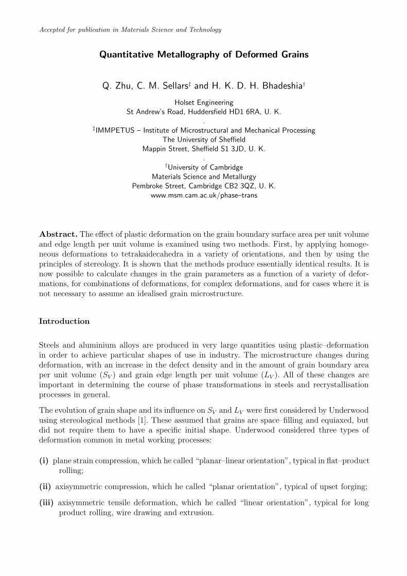
A tetrakaidecahedron has 8 hexagonal and 6 square faces, Fig. 1, with 36 edges, each of lengtha. All of the edges can be described in terms of just six vectors, as listed in Table 1. In previouswork [4], the axes of the deformation matrix were defined as illustrated in Fig. 1; in otherwords, the orientation of the grain was chosen in order to conveniently derive the deformationequations. This may be a weakness since in a real material the edges of the grains are likelyto be randomly oriented relative to the principal axes of the deformation. The purpose of thepresent work is to address these issues and to generalise the calculations to a greater variety ofindustrially important deformations, including redundant shear strains.

Throughout this work, it is assumed that the deformation is homogeneous; potential effectsof shear bands or mechanical twinning are not dealt with, nor is the creation of new high–misorientation boundaries by grain subdivision or by annealing twins losing coherency duringdeformation.

Fig. 1: Tetrakaidecahedron.

Quantitative Metallography of Deformed Grains 3

Table 1: Vectors defining the edges of a tetrakaidecahedron.

Vector Components

1 [a 0 0]

2 [0 a 0]

3 [−a2

−a2

a√2]

4 [a2

−a2

a√2]

5 [a2

a2

a√2]

6 [−a2

a2

a√2]

Analysis Method

Plane Strain Deformation A general deformation matrix S acts on a vector u to give anew vector v as follows [3, 4, 13]:

S11 S12 S13

S21 S22 S23

S31 S32 S33

u1

u2

u3

=

v1

v2

v3

(1)

Consider first the orientation of the tetrakaidecahedron as illustrated in Fig. 1. The tetrakaidec-ahedron is completely specified by the six initial vectors listed in Table 1. For plane strain de-formation, all Sij in equation 1 are zero except that S11 × S22 × S33 = 1 to conserve volume,and S11 × S33 = 1 since S22 = 1. For a diagonal matrix, the terms S11, S22 and S33 representthe principal distortions, i.e., the ratios of the final to initial lengths of unit vectors along theprincipal axes. It follows that for a diagonal S, the true strains are given by ε11 = lnS11,ε22 = lnS22 and ε33 = lnS33.

The application of the deformation to the initial set of vectors results in the new set of vectorslisted in Table 2. The latter are used to calculate the area and edge–lengths of the deformed ob-ject. Using equation 1 and the conditions for plane strain deformation, it can be shown that thefinal to initial area (A/A0) and edge–length (L/L0) ratios for the deformed tetrakaidecahedronare give by:

A

A0≡ SV

SV0

=S11 + 3(S11

√

1 + 2S233 +

√

S211 + 2S2

33) + S33

√

2(1 + S211)

3(2√

3 + 1)(2)

L

L0≡ LV

LV0

=1 + S11 + 2

√

1 + S211 + 2S2

33

6(3)

Here SV0and LV0

are the values at zero strain, of grain surface area and edge–length per unitvolume. These equations apply strictly to the grain orientation illustrated in Fig. 1, relative to


S. From stereology [1], SV0= 2/L so that SV

SV0

≡ 2SV L, and LV0= 9.088/L

2, where L is the

mean linear intercept commonly used to define the grain size [13, 14]. It follows that equations 2and 3 implicitly contain the grain size as an input variable.

Table 2: Components of the six vectors listed in Table 1, after plane strain or axisym-metric deformation.

Deformed Vector Components

1 [aS11 0 0]

2 [0 aS22 0]

3 [−aS11

2−aS22

2aS33√

2]

4 [aS11

2−aS22

2aS33√

2]

5 [aS11

2aS22

2aS33√

2]

6 [−aS11

2aS22

2aS33√

2]

The grain–orientation illustrated in Fig. 1 may not be representative. Suppose that we wish toorient the tetrakaidecahedron randomly with respect to the deformation. A rotation matrix Rcan be generated using random numbers to rotate the object relative to the axes defining S.Equation 1 then becomes

S11 S12 S13

S21 S22 S23

S31 S32 S33

R11 R12 R13

R21 R22 R23

R31 R32 R33

u1

u2

u3

=

v1

v2

v3

(4)

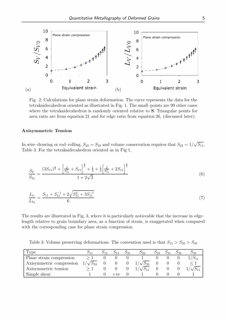
The results are illustrated in Fig. 2. For comparison purposes, the results are plotted againstthe equivalent strain:

ε =(

2

3

) 1

2

(

ε211 + ε2

22 + ε233 +

1

2γ2

13 +1

2γ2

12 +1

2γ2

23

) 1

2

(5)

where ε11, ε22, and ε33 are the normal components and γ13, γ12 and γ23 are the shear componentsof strain (the tangents of the shear angles). For homogeneous plane strain compression, ε =(2/

√3)ε11. In Fig. 2, the dashed line represents the outcome for the orientation illustrated in

Fig. 1 and the points are for the 99 other results of randomly oriented tetrakaidecahedra. It isclear that the orientation of the tetrakaidecahedron does not make much of a difference to theoutcome as far as the surface and edge–lengths per unit volume are concerned. This is probablybecause the tetrakaidecahedron is almost isotropic in shape.


(a) (b)

Fig. 2: Calculations for plane strain deformation. The curve represents the data for thetetrakaidecahedron oriented as illustrated in Fig. 1. The small–points are 99 other caseswhere the tetrakaidecahedron is randomly oriented relative to S. Triangular points forarea ratio are from equation 21 and for edge ratio from equation 26, (discussed later).

Axisymmetric Tension

In wire–drawing or rod–rolling, S22 = S33 and volume conservation requires that S22 = 1/√

S11,Table 3. For the tetrakaidecahedron oriented as in Fig 1,

SV

SV0

=(3S11)

1

2 +[

2S2

11

+ S11

]1

2

+ 13

+ 13

[

2S2

11

+ 2S11

]1

2

1 + 2√

3(6)

LV

LV0

=S11 + S−1

11 + 2√

S211 + 3S−1

11

6(7)

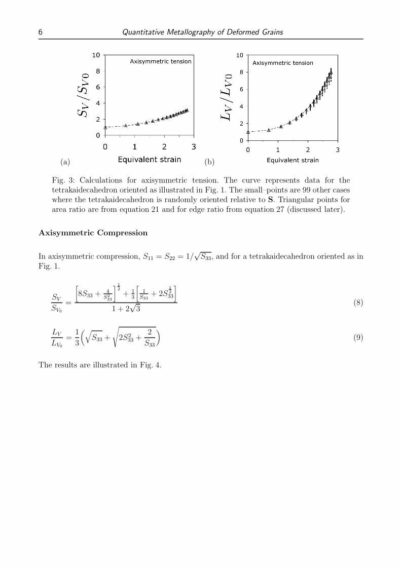
The results are illustrated in Fig. 3, where it is particularly noticeable that the increase in edge–length relative to grain boundary area, as a function of strain, is exaggerated when comparedwith the corresponding case for plane strain compression.

Table 3: Volume preserving deformations. The convention used is that S11 > S22 > S33

Type S11 S12 S13 S21 S22 S23 S31 S32 S33

Plane strain compression ≥ 1 0 0 0 1 0 0 0 1/S11

Axisymmetric compression 1/√

S33 0 0 0 1/√

S33 0 0 0 ≤ 1Axisymmetric tension ≥ 1 0 0 0 1/

√S11 0 0 0 1/

√S11

Simple shear 1 0 +ve 0 1 0 0 0 1


(a) (b)

Fig. 3: Calculations for axisymmetric tension. The curve represents data for thetetrakaidecahedron oriented as illustrated in Fig. 1. The small–points are 99 other caseswhere the tetrakaidecahedron is randomly oriented relative to S. Triangular points forarea ratio are from equation 21 and for edge ratio from equation 27 (discussed later).

Axisymmetric Compression

In axisymmetric compression, S11 = S22 = 1/√

S33, and for a tetrakaidecahedron oriented as inFig. 1.

SV

SV0

=

[

8S33 + 4S2

33

]1

2

+ 13

[

1S33

+ 2S1

2

33

]

1 + 2√

3(8)

LV

LV0

=1

3

(

√

S33 +

√

2S233 +

2

S33

)

(9)

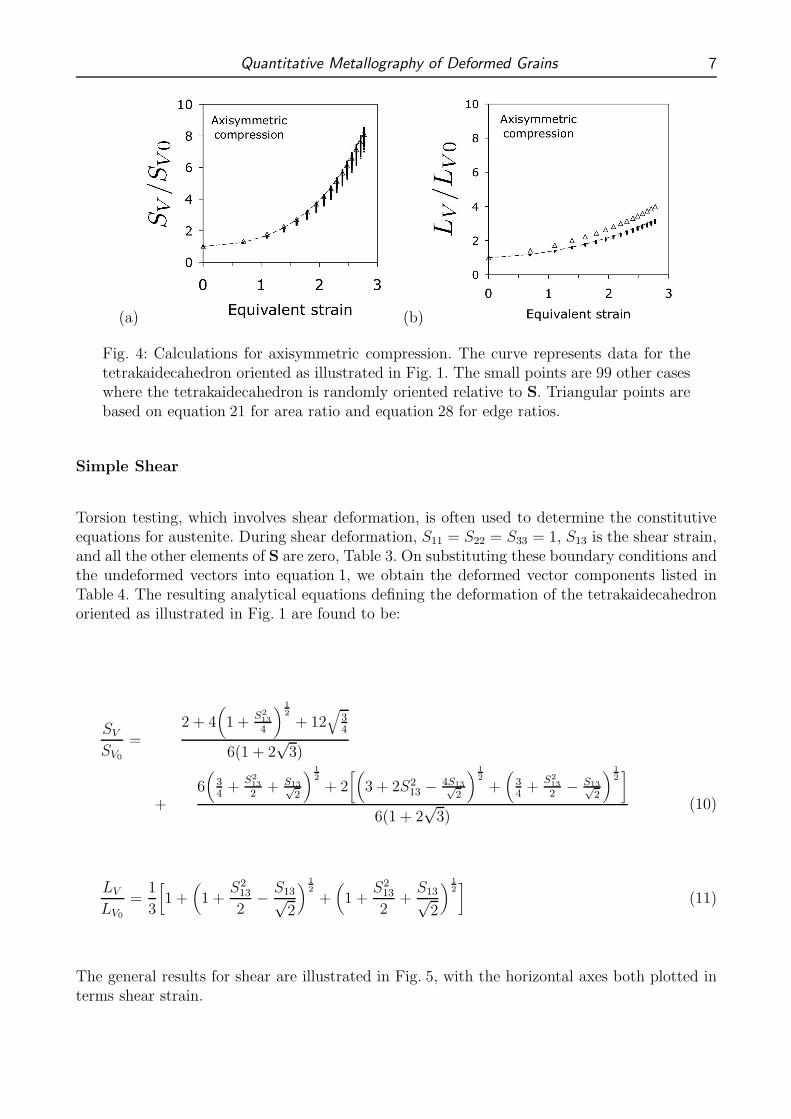
The results are illustrated in Fig. 4.


(a) (b)

Fig. 4: Calculations for axisymmetric compression. The curve represents data for thetetrakaidecahedron oriented as illustrated in Fig. 1. The small points are 99 other caseswhere the tetrakaidecahedron is randomly oriented relative to S. Triangular points arebased on equation 21 for area ratio and equation 28 for edge ratios.

Simple Shear

Torsion testing, which involves shear deformation, is often used to determine the constitutiveequations for austenite. During shear deformation, S11 = S22 = S33 = 1, S13 is the shear strain,and all the other elements of S are zero, Table 3. On substituting these boundary conditions andthe undeformed vectors into equation 1, we obtain the deformed vector components listed inTable 4. The resulting analytical equations defining the deformation of the tetrakaidecahedronoriented as illustrated in Fig. 1 are found to be:

SV

SV0

=2 + 4

(

1 +S2

13

4

) 1

2

+ 12√

34

6(1 + 2√

3)

+6(

34

+S2

13

2+ S13√

2

) 1

2

+ 2[(

3 + 2S213 − 4S13√

2

) 1

2

+(

34

+S2

13

2− S13√

2

) 1

2

]

6(1 + 2√

3)(10)

LV

LV0

=1

3

[

1 +(

1 +S2

13

2− S13√

2

) 1

2

+(

1 +S2

13

2+

S13√2

) 1

2

]

(11)

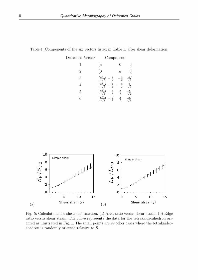
The general results for shear are illustrated in Fig. 5, with the horizontal axes both plotted interms shear strain.


Table 4: Components of the six vectors listed in Table 1, after shear deformation.

Deformed Vector Components

1 [a 0 0]

2 [0 a 0]

3 [aS13√2− a

2−a

2a√2]

4 [aS13√2

+ a2

−a2

a√2]

5 [aS13√2

+ a2

a2

a√2]

6 [aS13√2− a

2a2

a√2]

(a) (b)

Fig. 5: Calculations for shear deformation. (a) Area ratio versus shear strain. (b) Edgeratio versus shear strain. The curve represents the data for the tetrakaidecahedron ori-ented as illustrated in Fig. 1. The small points are 99 other cases where the tetrakaidec-ahedron is randomly oriented relative to S.


Sequential Deformations

The method here is general – all that is needed is to define the matrix S for the appropriatecircumstances. There are cases where two or more different kinds of deformation are used insequence, for example, cross–rolling in which the plate is rotated through 90 after a degree ofreduction. This is readily tackled by generalising equation 1. Rotation through 90 about thecompression axis [0 0 1] is given by [13]:

R =

0 1 0−1 0 00 0 1

(12)

Writing the first rolling pass as S and the cross–rolling pass as T, the net deformation U isgiven by TRS:

U =

T11 0 00 1 00 0 1/T11

0 1 0−1 0 00 0 1

S11 0 00 1 00 0 1/S11

=

0 T11 0−S11 0 0

0 0 1T11S11

(13)

Complex Deformations

Flat product rolling is approximated as plane strain compression, but friction with the rollsleads to shears. The plane strain condition is strictly satisfied only at the centre of the rolledmaterial. The matrix S can be used to deal with the simultaneous actions of plane straincompression and simple shear (on the rolling plane and in the rolling direction) by generalisingthe deformation matrix equation 1 as follows:

S11 0 S ′13

0 1 00 0 1/S11

(14)

The final shear strain S ′13 arises from the imposed shear strain, S13, modified by the compression

S11 and is represented by S13 × S11.

Meterology

As pointed out in the introduction, real microstructures will contain a distribution of grainsizes. This is enshrined on a statistical basis in stereological parameters such as the mean linearintercept L etc. It is useful therefore, to see whether the outcomes discussed in the previoussections can be reproduced using stereology.

The volume, surface area and edge length of an undeformed tetrakaidecahedron, Fig. 1, aregiven by:

V0 = 8√

2a3 S0 = 6(1 + 2√

3)a2 and L0 = 36a (15)


It follows that for a uniform grain structure

SV0=

3(1 + 2√

3)

8√

2aand LV0

=3

2√

2a2(16)

The mean linear intercept representing the undeformed grain size measured on two–dimensionalsections therefore becomes

L0 =2

SV0

=16√

2a

3(1 + 2√

3)(17)

For a deformed grain, given that the number of boundaries per unit length NL1 ≤ NL2 ≤ NL3,the surface per unit volume from [1] is:

SV = 0.429NL1 + 0.571NL2 + NL3 (18)

and since L = 1/N , for plastic deformation in which ε11 ≥ ε22 ≥ ε33, the linear intercepts are

L1 = L0 expε11 L2 = L0 expε22 L3 = L0 expε33 (19)

so that

SV = L−10 (0.429 exp−ε11 + 0.571 exp−ε22 + exp−ε33) (20)

SV

SV0

=1

2(0.429 exp−ε11 + 0.571 exp−ε22 + exp−ε33) (21)

This equation can be used in association with the boundary conditions outlined in Table 5 toestimate SV for a variety of deformations. In Figs. 2a, 3a and 4a, the triangular points arecalculated using equation 21.

Table 5: Strains for substitution into equations 20 and 21. Note that ε11 + ε22 + ε33 mustequal zero to conserve volume, and it is assumed that ε11 ≥ ε22 ≥ ε33.

Deformation ε11 ε22 ε33

Plane strain compression +ve 0 -ε11

Axisymmetric tension +ve −12ε11 −1

2ε11

Axisymmetric compression −12ε33 −1

2ε33 −ve

When dealing with oriented structures, lines in a given volume can be categorised into segmentswhich are aligned parallel to one or more directions, with the remainder being randomly oriented[1]. For the anisotropic grains which result from plane strain compression (planar–linear oriented


structure [1]), the edge–length per unit volume is the sum of three contributions from isometric(randomly oriented), planar (compressed) and linear elements (elongated) components [1]:

LV = LVisometric+ LVplanar

+ LVlinear(22)

For an undeformed tetrakaidecahedron, the relationship between the edge length per unit vol-ume and the number of points of intersections of edges with a test plane of unit area is simple,LV = 2PA [1]. For a deformed grain it is necessary to specify the three contributions of equa-tion 22. If ‘1’ and ‘3’ are the rolling and thickness directions respectively, then from [1],

LVisometric= 2PA3

LVplanar= (PA1

− PA3) LVlinear

=1

2(PA2

− PA3) (23)

where PA3refers to the points per unit area on the plane normal to the 3–axis etc. It follows

that

LV = PA3+

1

2[PA1

+ PA2] (24)

with

PA1= PA exp−(ε22 + ε33)

PA2= PA exp−(ε11 + ε33)

PA3= PA exp−(ε11 + ε22) (25)

By combining these equations we obtain for plane strain deformation,

LV

LV0

=1

4exp−ε11 +

1

4exp−ε22 +

1

2exp−ε33 (26)

The results obtained using this equation are plotted as triangular points on Fig. 2b, showinggood agreement with the data from equation 3.

Axisymmetric tension is described as a linearly–oriented structure so the planar component inequation 22 is absent, resulting in a different equation for edge–length per unit volume. Given1 and 3 as the longitudinal and radial directions respectively, we have (equation 3.15, [1]):

LV = PA1+ PA3

= PA0[expε11 + exp−ε11/2]

LV

LV0

=1

2(exp−2ε33 + expε33) (27)

The excellent agreement between the different methods is illustrated in Fig. 3b.

Axisymmetric compression effectively flattens the grains normal to the compression axis andhence leads to what Underwood calls a planar oriented structure (Fig. 3.13, [1]). The values of


PA in the planes containing the compression axis grow rapidly whereas they decline rapidly inthose normal to the compression axis. This is difficult to treat, because the degree of orientation(Ω in Underwood’s terminology [1]) becomes negative. This is not the case for axisymmetric ten-sion. However, if it is assumed as an approximation that the planes containing the compressionaxis dominate, then

LV

LV0

' exp−(ε22 + ε33) (28)

The results of these calculations are illustrated as triangular points on Fig. 4, and, unusu-ally compared with other deformation conditions, they lie above the maxiumum value for thetetrakaidecahedra because of the approximation in equation 28.

Discussion

Deformation Mode In order to determine the flow stress and dislocation structures relevantfor industrial hot working conditions, tension, axisymmetric compression, plane strain compres-sion and torsion tests are used by different research groups. It is generally considered that resultsfrom the different tests are consistent when they are compared at the same equivalent strainfor tests at the same equivalent strain rate and temperature. The dislocation structures providethe driving force for nucleation and growth of recrystallised grains formed either dynamicallyor statically. In both cases nucleation occurs preferentially at grain boundaries, with grainedges being important at low strains, but grain surfaces being more important over most ofthe range of strains of interest in industrial hot working operations [15]. Comparing the effectsof equivalent strain on SV /SV0

and LV /LV0for plane strain compression, axisymmetric tension

and axisymmetric compression in Figs. 2, 3 and 4, it can be seen that the maximum values fortetrakaidecahedra correspond closely with the results from the metrology analysis. The valuesof SV /SV0

also correspond closely with the results for the deformation of spheres computedby Bate and Hutchinson [9], who showed that their analysis always gave higher values thananalyses for the deformation of cubes [10–12]. In this context, it is of interest to note that theminimum values from the present analysis of tetrakaidecahedra are also always above the valuesfor cubes. In further discussion, only the maximum values given by equations 2 and 3, 6 and 7and 8 and 9 will be considered.

The present results for SV /SV0and LV /LV0

in axisymmetric tension (long product rolling,wire drawing and extrusion), Fig. 3, and in axisymmetric compression (upset forging), Fig. 4,are antisymmetric, so tension is much less effective than compression in increasing SV /SV0

and vice versa for increasing LV /LV0. Also, axisymmetric compression is more effective in

increasing SV /SV0than plane strain compression (flat product rolling), Fig. 2. This difference

arises mainly from the influence of the different constraints on the values of equivalent strainfor a given reduction in height (ε33).

For simple shear, the results in Fig. 5 are plotted against the shear strain (γ = S13), becausethere is some controversy about how shear strains should be converted to equivalent strains.Equation 5, leading to ε = γ/

√3, is valid for small strains, and Canova et al. [16] argued that

it is also valid for large strains. This view is frequently adopted for analysis of the results fromtorsion tests and from the effects of redundant shear strains in rolling and extrusion, However,


Bate and Hutchinson [9] derived a relationship for the equivalent strain from the initial andfinal states after simple shear deformation of spheres as follows:

ε =2√3

ln[

γ

2+

(

1 +γ2

4

)] 1

2

(29)

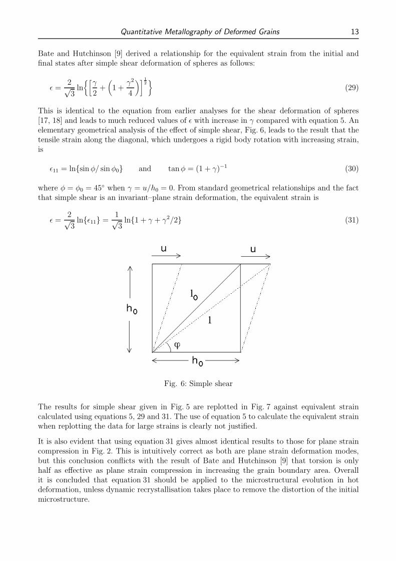
This is identical to the equation from earlier analyses for the shear deformation of spheres[17, 18] and leads to much reduced values of ε with increase in γ compared with equation 5. Anelementary geometrical analysis of the effect of simple shear, Fig. 6, leads to the result that thetensile strain along the diagonal, which undergoes a rigid body rotation with increasing strain,is

ε11 = lnsin φ/ sin φ0 and tanφ = (1 + γ)−1 (30)

where φ = φ0 = 45 when γ = u/h0 = 0. From standard geometrical relationships and the factthat simple shear is an invariant–plane strain deformation, the equivalent strain is

ε =2√3

lnε11 =1√3

ln1 + γ + γ2/2 (31)

Fig. 6: Simple shear

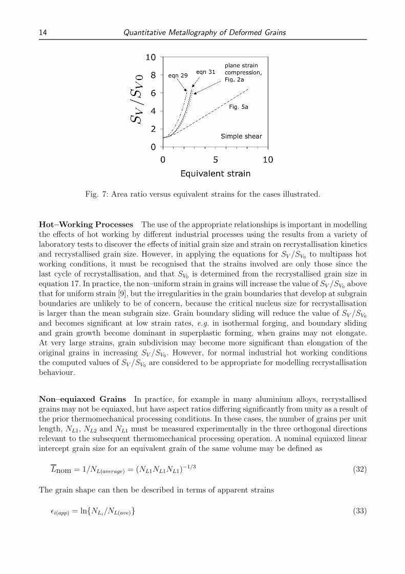
The results for simple shear given in Fig. 5 are replotted in Fig. 7 against equivalent straincalculated using equations 5, 29 and 31. The use of equation 5 to calculate the equivalent strainwhen replotting the data for large strains is clearly not justified.

It is also evident that using equation 31 gives almost identical results to those for plane straincompression in Fig. 2. This is intuitively correct as both are plane strain deformation modes,but this conclusion conflicts with the result of Bate and Hutchinson [9] that torsion is onlyhalf as effective as plane strain compression in increasing the grain boundary area. Overallit is concluded that equation 31 should be applied to the microstructural evolution in hotdeformation, unless dynamic recrystallisation takes place to remove the distortion of the initialmicrostructure.


Fig. 7: Area ratio versus equivalent strains for the cases illustrated.

Hot–Working Processes The use of the appropriate relationships is important in modellingthe effects of hot working by different industrial processes using the results from a variety oflaboratory tests to discover the effects of initial grain size and strain on recrystallisation kineticsand recrystallised grain size. However, in applying the equations for SV /SV0

to multipass hotworking conditions, it must be recognised that the strains involved are only those since thelast cycle of recrystallisation, and that SV0

is determined from the recrystallised grain size inequation 17. In practice, the non–uniform strain in grains will increase the value of SV /SV0

abovethat for uniform strain [9], but the irregularities in the grain boundaries that develop at subgrainboundaries are unlikely to be of concern, because the critical nucleus size for recrystallisationis larger than the mean subgrain size. Grain boundary sliding will reduce the value of SV /SV0

and becomes significant at low strain rates, e.g. in isothermal forging, and boundary slidingand grain growth become dominant in superplastic forming, when grains may not elongate.At very large strains, grain subdivision may become more significant than elongation of theoriginal grains in increasing SV /SV0

. However, for normal industrial hot working conditionsthe computed values of SV /SV0

are considered to be appropriate for modelling recrystallisationbehaviour.

Non–equiaxed Grains In practice, for example in many aluminium alloys, recrystallisedgrains may not be equiaxed, but have aspect ratios differing significantly from unity as a result ofthe prior thermomechanical processing conditions. In these cases, the number of grains per unitlength, NL1, NL2 and NL1 must be measured experimentally in the three orthogonal directionsrelevant to the subsequent thermomechanical processing operation. A nominal equiaxed linearintercept grain size for an equivalent grain of the same volume may be defined as

Lnom = 1/NL(average) = (NL1NL1NL1)−1/3 (32)

The grain shape can then be described in terms of apparent strains

εi(app) = lnNLi/NL(ave) (33)


The effect of subsequent normal strain components can then simply be found, e.g. from equa-tion 22, by replacing the applied strain components, εi by εi+εi(app). This simple analysis appliesonly when the axes of the elongated grain shape are the same as those of the subsequent de-formation. It is also possible to have elongated grain structures that are not related to thedeformation axes.

One example where the initial grain structure is highly elongated is the plate shape observedin martensitic microstructures. The method presented here is able to deal with this as long asthe initial structure can be represented by a set of vectors.

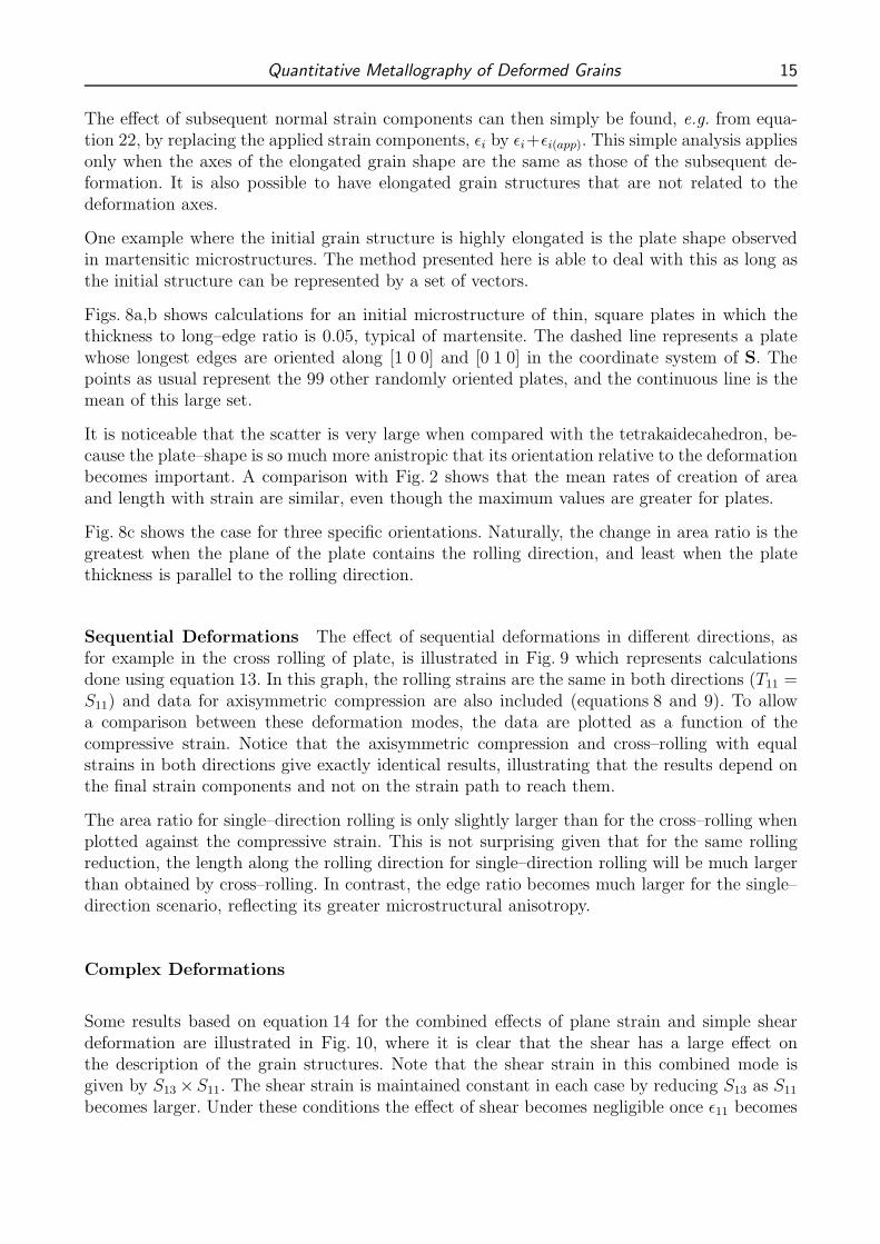
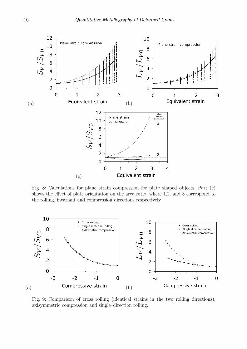
Figs. 8a,b shows calculations for an initial microstructure of thin, square plates in which thethickness to long–edge ratio is 0.05, typical of martensite. The dashed line represents a platewhose longest edges are oriented along [1 0 0] and [0 1 0] in the coordinate system of S. Thepoints as usual represent the 99 other randomly oriented plates, and the continuous line is themean of this large set.

It is noticeable that the scatter is very large when compared with the tetrakaidecahedron, be-cause the plate–shape is so much more anistropic that its orientation relative to the deformationbecomes important. A comparison with Fig. 2 shows that the mean rates of creation of areaand length with strain are similar, even though the maximum values are greater for plates.

Fig. 8c shows the case for three specific orientations. Naturally, the change in area ratio is thegreatest when the plane of the plate contains the rolling direction, and least when the platethickness is parallel to the rolling direction.

Sequential Deformations The effect of sequential deformations in different directions, asfor example in the cross rolling of plate, is illustrated in Fig. 9 which represents calculationsdone using equation 13. In this graph, the rolling strains are the same in both directions (T11 =S11) and data for axisymmetric compression are also included (equations 8 and 9). To allowa comparison between these deformation modes, the data are plotted as a function of thecompressive strain. Notice that the axisymmetric compression and cross–rolling with equalstrains in both directions give exactly identical results, illustrating that the results depend onthe final strain components and not on the strain path to reach them.

The area ratio for single–direction rolling is only slightly larger than for the cross–rolling whenplotted against the compressive strain. This is not surprising given that for the same rollingreduction, the length along the rolling direction for single–direction rolling will be much largerthan obtained by cross–rolling. In contrast, the edge ratio becomes much larger for the single–direction scenario, reflecting its greater microstructural anisotropy.

Complex Deformations

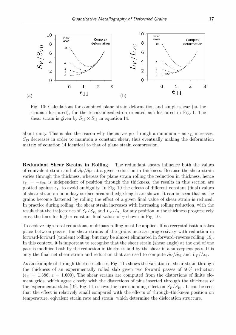
Some results based on equation 14 for the combined effects of plane strain and simple sheardeformation are illustrated in Fig. 10, where it is clear that the shear has a large effect onthe description of the grain structures. Note that the shear strain in this combined mode isgiven by S13 ×S11. The shear strain is maintained constant in each case by reducing S13 as S11

becomes larger. Under these conditions the effect of shear becomes negligible once ε11 becomes


(a) (b)

(c)

Fig. 8: Calculations for plane strain compression for plate–shaped objects. Part (c)shows the effect of plate orientation on the area ratio, where 1,2, and 3 correspond tothe rolling, invariant and compression directions respectively.

(a) (b)

Fig. 9: Comparison of cross–rolling (identical strains in the two rolling directions),axisymmetric compression and single–direction rolling.


(a) (b)

Fig. 10: Calculations for combined plane strain deformation and simple shear (at thestrains illustrated), for the tetrakaidecahedron oriented as illustrated in Fig. 1. Theshear strain is given by S13 × S11 in equation 14.

about unity. This is also the reason why the curves go through a minimum – as ε11 increases,S13 decreases in order to maintain a constant shear, thus eventually making the deformationmatrix of equation 14 identical to that of plane strain compression.

Redundant Shear Strains in Rolling The redundant shears influence both the valuesof equivalent strain and of SV /SV0

at a given reduction in thickness. Because the shear strainvaries through the thickness, whereas for plane strain rolling the reduction in thickness, henceε11 = −ε33, is independent of position through the thickness, the results in this section areplotted against ε11 to avoid ambiguity. In Fig. 10 the effects of different constant (final) valuesof shear strain on boundary surface area and edge length are shown. It can be seen that as thegrains become flattened by rolling the effect of a given final value of shear strain is reduced.In practice during rolling, the shear strain increases with increasing rolling reduction, with theresult that the trajectories of SV /SV0

and LV /LV0for any position in the thickness progressively

cross the lines for higher constant final values of γ shown in Fig. 10.

To achieve high total reductions, multipass rolling must be applied. If no recrystallisation takesplace between passes, the shear strains of the grains increase progressively with reduction inforward-forward (tandem) rolling, but may be almost eliminated in forward–reverse rolling [19].In this context, it is important to recognise that the shear strain (shear angle) at the end of onepass is modified both by the reduction in thickness and by the shear in a subsequent pass. It isonly the final net shear strain and reduction that are used to compute SV /SV0

and LV /LV0.

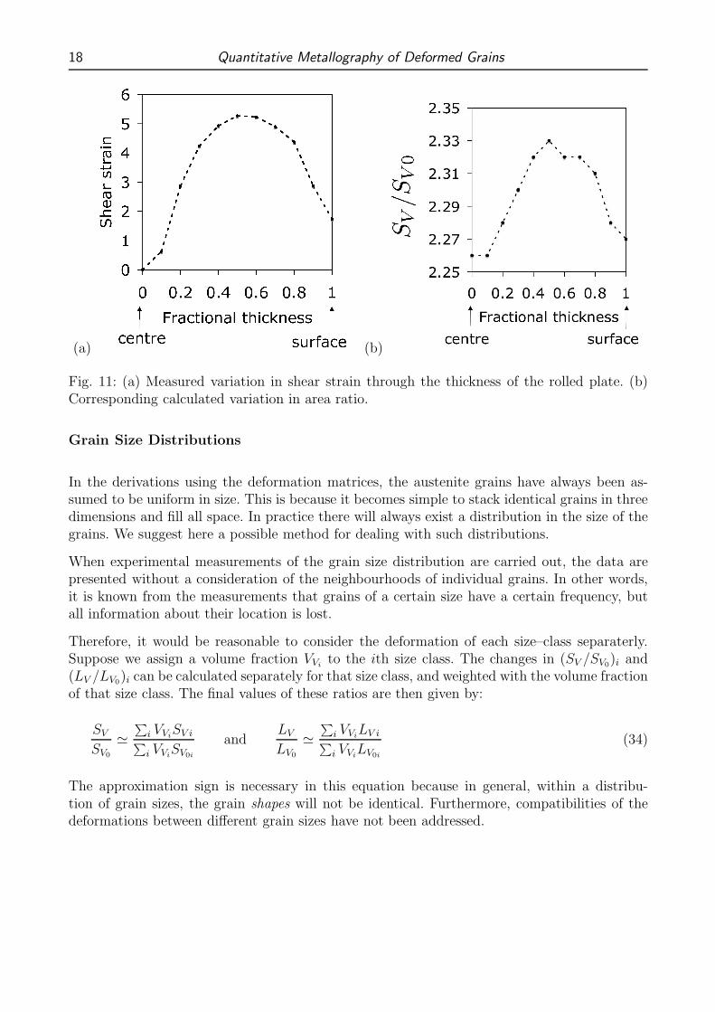
As an example of through-thickness effects, Fig. 11a shows the variation of shear strain throughthe thickness of an experimentally rolled slab given two forward passes of 50% reduction(ε11 = 1.386, ε = 1.600). The shear strains are computed from the distortions of finite ele-ment grids, which agree closely with the distortions of pins inserted through the thickness ofthe experimental slabs [19]. Fig. 11b shows the corresponding effect on SV /SV0

. It can be seenthat the effect is relatively small compared with the effects of through–thickness position ontemperature, eqivalent strain rate and strain, which determine the dislocation structure.


(a) (b)

Fig. 11: (a) Measured variation in shear strain through the thickness of the rolled plate. (b)Corresponding calculated variation in area ratio.

Grain Size Distributions

In the derivations using the deformation matrices, the austenite grains have always been as-sumed to be uniform in size. This is because it becomes simple to stack identical grains in threedimensions and fill all space. In practice there will always exist a distribution in the size of thegrains. We suggest here a possible method for dealing with such distributions.

When experimental measurements of the grain size distribution are carried out, the data arepresented without a consideration of the neighbourhoods of individual grains. In other words,it is known from the measurements that grains of a certain size have a certain frequency, butall information about their location is lost.

Therefore, it would be reasonable to consider the deformation of each size–class separaterly.Suppose we assign a volume fraction VVi

to the ith size class. The changes in (SV /SV0)i and

(LV /LV0)i can be calculated separately for that size class, and weighted with the volume fraction

of that size class. The final values of these ratios are then given by:

SV

SV0

'∑

i VViSV i

∑

i VViSV0i

andLV

LV0

'∑

i VViLV i

∑

i VViLV0i

(34)

The approximation sign is necessary in this equation because in general, within a distribu-tion of grain sizes, the grain shapes will not be identical. Furthermore, compatibilities of thedeformations between different grain sizes have not been addressed.


Conclusions

Two quite different approaches to the quantitative metallography of deformed grains produceessentially identical results. The methodology in which a homogeneous deformation is applied toa particular shape is versatile in that equation 1 can in principle be applied to any grain–shapeor process, including others not covered in this paper.

The software associated with all the calculations can be obtained freely from

www.msm.cam.ac.uk/map/mapmain.html

References

[1] E. E. Underwood. Quantitative Stereology. Addison–Wesley Publication Company, 1970.

[2] Y. van Leeuwen, S. Vooijs, J. Sietsma, and S. Van der Zwaag. Effect of geometrical as-sumptions in modelling solid state kinetics. Metallurgical & Materials Transactions A,29:2925–2931, 1998.

[3] I. Czinege and T. Reti. Determination of local deformation in cold formed products by ameasurement of the geometric characteristics of the crystallites. In Eighteenth InternationalMachine Tool Design and Research Conference, Forming, volume 1, pages 159–163, 1977.

[4] S. B. Singh and H. K. D. H. Bhadeshia. Topology of grain deformation. Materials Scienceand Technology, 15:832–834, 1998.

[5] K. Matsuura and Y. Itoh. Estimation of three-dimensional grain size distribution in poly-crystalline material. Materials Transactions JIM, 32:1042–1047, 1991.

[6] Y. Takayama, N. Furushiro, T. Tozawa, H. Kato, and S. Hori. A significant method forestimation of the grain size of polycrystalline materials. Materials Transactions JIM,32:214–221, 1991.

[7] P. L. Orsetti Rossi and C. M. Sellars. Quantitative metallography of recrystallization. ActaMaterialia, 45:137–148, 1997.

[8] M. Umemoto, H. Ohtsuka, and I. Tamura. Transformation to pearlite from work hardenedaustenite. Trans. ISIJ, 23:775–784, 1983.

[9] P. Bate and W. B. Hutchinson. Grain boundary area and deformation. Scripta Materialia,52:199–203, 2005.

[10] J. Gil-Sevillano, P. van Houtte, and E. Aernoudt. Large strain work hardening and tex-tures. Progress in Materials Science, 27:69–314, 1980.

[11] H. E. Vatne, T. Furu, R. Ørsund, and E. Nes. Modelling recrystallization after hot defor-mation of aluminium. Acta Materialia, 44:4463–4473, 1996.

[12] O. Knustad, H. J. McQueen, N. Ryum, and J. K. Solberg. . Practical Metallography, 22:215,1985.


[13] H. K. D. H. Bhadeshia. Geometry of Crystals. 2nd edition, Institute of Materials, 2001.

[14] C. Mack. Proceedings of the Cambridge Philosophical Society, 52:286, 1956.

[15] C. M. Sellars. . In B. Hutchinson et al., editor, Proc. Int. Conf. Thermomechanical Pro-cessing: Theory, Modelling and Practice [TMP], Stockholm, pages 35–51, 1997.

[16] G. R. Canova, S. Chrivastava, J. J. Jonas, and C. G’Sell. . In J. R. Newby and B. A.Niemeir, editors, Formability of Metallic Materials – 2000AD, ASTM STP 753, pages1889–210, 1982.

[17] A. Nadai and E. Davis. Plastic behavior of metals in the strain-hardening range. Journalof Applied Physics, 8:205–217, 1937.

[18] A. Eichinger. Werkstoffprufung, volume 2, p. 715. Springer–Verlag, Berlin, Germany, 1955.

[19] A. Mukhopadhyay, R. L. Higginson, I. C. Howard, and C. M. Sellars. . Materials Scienceand Technology, page in press, 2006.

quantitative metallography of deformed grains · quantitative metallography of deformed grains 3...

Documents