quantitative investment: research and implementation in matlab€¦ · quantitative investment:...

Quantitative Investment:Research and Implementation in MATLAB

Edward Hoyle

Fulcrum Asset Management6 Chesterfield Gardens

London, W1J 5BQ

[email protected]

24 June 2014MATLAB Computational Finance Conference 2014

Etc Venues, St Paul’s, London

Edward Hoyle (Fulcrum) Quantitative Investment 24 June 2014, London 1 / 25

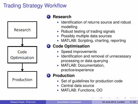
Trading Strategy Workflow

1 ResearchI Identification of returns source and robust

modellingI Robust testing of trading signalsI Possibly multiple data sourcesI MATLAB: Scripting, charting, reporting

2 Code OptimisationI Speed improvementsI Identification and removal of unnecessary

processing or data queryingI MATLAB: Documentation,

practice/experience3 Production

I Set of guidelines for production codeI Central data sourceI MATLAB: Functions, OO


Generic Trading Strategy1 Data

I Historical and real-timeI Financial, economic, sentiment, etc.

2 ModelI Simplification of reality which captures

certain important featuresI E.g. use inflation and growth to forecast

bond yieldsI E.g. high-yielding currencies appreciate

against low-yielding currenciesI E.g. asset-price trends are persistent

3 Trading signalI Convert model outputs into trading positionsI Which assets to buy and sell, and in what

quantitiesI Position sizing may be dependent on risk or

regulatory constraints


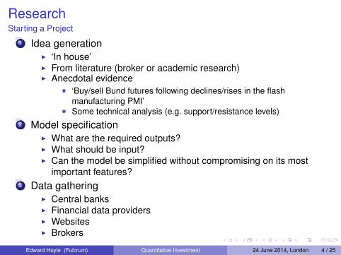
ResearchStarting a Project

1 Idea generationI ‘In house’I From literature (broker or academic research)I Anecdotal evidence

F ‘Buy/sell Bund futures following declines/rises in the flashmanufacturing PMI’

F Some technical analysis (e.g. support/resistance levels)2 Model specification

I What are the required outputs?I What should be input?I Can the model be simplified without compromising on its most

important features?3 Data gathering

I Central banksI Financial data providersI WebsitesI Brokers


Personal Modelling PhilosophyA Digression

I learnt this the hard way:

If a simple trading model can be shown to work, acomplicated model may improve results.

If no simple trading model can be shown to work, nocomplicated model will improve results.

This does not mean that building successful trading models is easy. Asis typical in research, 90% of the work is finding the right questions toask; the other 10% is finding answers.


ResearchFitting Models

Robustness checksSensitivity of model output to parametersStability of parameters

I Do different fitting methods produce similar results?I How sensitive are parameters to the data sample?

Are we sure there is no peek-ahead bias?I This is particular concern for models using macroeconomic

variablesI Have historical data been adjusted retrospectively?I Have data release delays been accounted for?I Have differing market trading hours (S&P versus Nikkei) been

accounted for?


ResearchIdentifying Trading Signals

Demonstrate that a trading signal has predictive powerI This is often quite hard!I A successful backtest alone does not usually convince meI Charts can be very useful here

Robustness checksI Do the signals have a directional bias? Should they?I Are signals effective after accounting for market trends?I Are both the long and short signals profitable?I Does a stronger signal have stronger forecasting power? Should it?


ResearchTrading Strategy

BacktestingI DrawdownsI Performance metricsI Persistence (across markets, across subsamples)

DependenciesI Correlations with other strategies

RobustnessI Sensitivity to parametersI Regime analysis

F rising/falling interest ratesF economic growth/recessionF bull/bear market

Adding to a broader portfolioI Effect on the portfolio’s leverage?I Effect on the portfolio’s risk allocation to assets and asset classes?I Effect on the portfolio’s volatility/VaR/expected shortfall?


Code Optimisation

Code optimisation by exampleA real-world code-optimisation problemThe code solved a constrained minimisation problemI shall show some of the steps taken to improve the efficiency andreliability of the solverA particular concern was to ensure that the solution was notsensitive to the starting point of the minimisationSpeed was an important consideration here, but was secondary torobustnessNote: The Parallel Computing Toolbox was not used whenproducing the following results (although it would probably havesped things up)


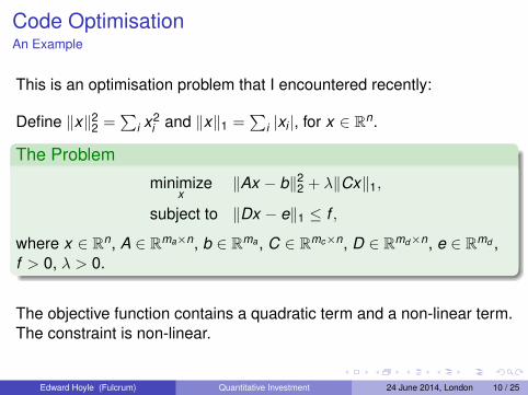
Code OptimisationAn Example

This is an optimisation problem that I encountered recently:

Define ‖x‖22 =∑

i x2i and ‖x‖1 =

∑i |xi |, for x ∈ Rn.

The Problem

minimizex

‖Ax − b‖22 + λ‖Cx‖1,

subject to ‖Dx − e‖1 ≤ f ,

where x ∈ Rn, A ∈ Rma×n, b ∈ Rma , C ∈ Rmc×n, D ∈ Rmd×n, e ∈ Rmd ,f > 0, λ > 0.

The objective function contains a quadratic term and a non-linear term.The constraint is non-linear.


Code OptimisationFirst Attempt

Don’t work harder than you need to!Use fmincon (Optimization Toolbox)Very quick to set up the problem


Code OptimisationPerformance: Naive fmincon

20 dimensional problem100 different random starting points (not necessarily satisfyingconstraints)Timing = 1,144.92 secondsObjective: mean 2.1152, min 2.0951, max 2.1532

Table: Values for x1, . . . , x5.

i Mean Min Max SD

1 0.2932 0.2559 0.3120 0.01252 1.9193 1.7683 2.2189 0.12823 -0.7701 -1.5355 -0.2690 0.35284 4.5681 4.2161 4.8536 0.11805 0.5654 0.4741 0.7047 0.0464


Code OptimisationSecond Attempt

We like the results from the first attemptCan we improve performance or robustness?Supply gradients for the objective and constraint usingoptions = optimoptions('fmincon'...

, 'GradObj', 'on', 'GradConstr', 'on')

∇{‖Dx − e‖1} = D′sign(Dx − e)

∇{‖Ax − b‖22 + λ‖Cx‖1

}= 2A′Ax − 2A′b + λC′sign(Cx)

Note: There are many other fmincon options that can be changedin the bid to improve performance


Code OptimisationPerformance: fmincon with gradients

20 dimensional problem100 different random starting points (not necessarily satisfyingconstraints)Timing = 96.04 seconds (92.1% speed up)Objective: mean 2.1153, min 2.0948, max 2.1865


i Mean Min Max SD

1 0.2939 0.2559 0.3128 0.01262 1.9119 1.7768 2.2191 0.12553 -0.7636 -1.7491 -0.2658 0.34364 4.5720 4.2160 4.8536 0.11745 0.5659 0.4745 0.7047 0.0447


Code OptimisationQ. How Can We Improve Further? A. Do Some Research!

Boyd & VandenbergheCambridge University PressAlso available at http://www.stanford.edu/~boyd/cvxbook/


http://www.stanford.edu/~boyd/cvxbook/

http://www.stanford.edu/~boyd/cvxbook/

Code OptimisationThe Problem Revisited

Find an optimisation problem with the same optimal solution, but with a‘nicer’ form:

Equivalent Problem

minimizex ,u,t

x ′A′Ax − 2A′bx + λ1′t

subject to −t � Cx � t ,−u � Dx − e � u,1′u ≤ f ,

where t ∈ Rmc+ , u ∈ Rmd

+ .

The objective function is quadraticThe constraints are linearWe can use quadprog (Optimization Toolbox)


Code OptimisationPerformance: quadprog

20 dimensional problem100 different random starting points (not necessarily satisfyingconstraints)Timing = 1.34 seconds (99.9% speed up)Objective: mean 2.0041, min 2.0041, max 2.0041


i Mean Min Max SD

1 0.2917 0.2917 0.2917 0.00002 1.7458 1.7458 1.7458 0.00003 0.0141 0.0141 0.0141 0.00004 4.5358 4.5358 4.5358 0.00005 0.5095 0.5095 0.5095 0.0000


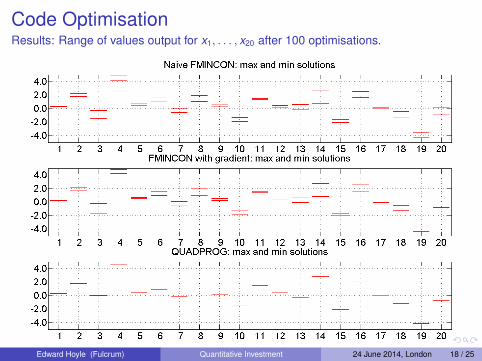
Code OptimisationResults: Range of values output for x1, . . . , x20 after 100 optimisations.


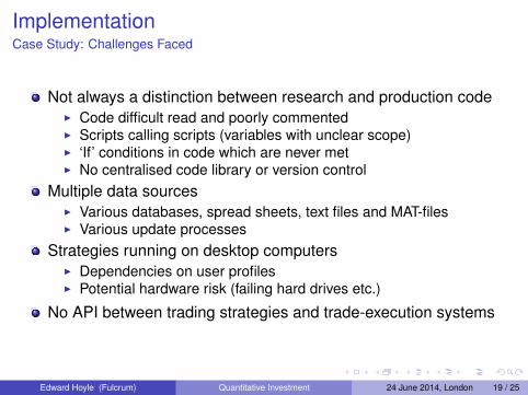
ImplementationCase Study: Challenges Faced

Not always a distinction between research and production codeI Code difficult read and poorly commentedI Scripts calling scripts (variables with unclear scope)I ‘If’ conditions in code which are never metI No centralised code library or version control

Multiple data sourcesI Various databases, spread sheets, text files and MAT-filesI Various update processes

Strategies running on desktop computersI Dependencies on user profilesI Potential hardware risk (failing hard drives etc.)

No API between trading strategies and trade-execution systems


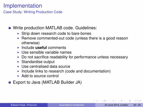
ImplementationCase Study: Writing Production Code

Write production MATLAB code. Guidelines:I Strip down research code to bare bonesI Remove commented-out code (unless there is a good reason

otherwise)I Include useful commentsI Use sensible variable namesI Do not sacrifice readability for performance unless necessaryI Standardise outputI Use centralised data sourceI Include links to research (code and documentation)I Add to source control

Export to Java (MATLAB Builder JA)


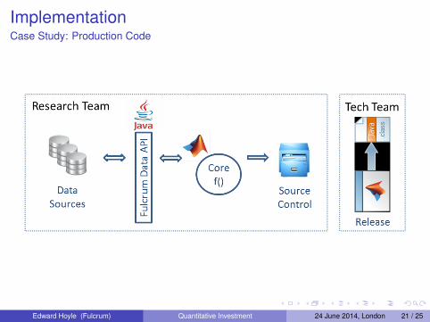
ImplementationCase Study: Production Code


ImplementationCase Study: Production Environment

Java platform for the execution of medium-frequency trades:1 Update central database2 Run MATLAB strategies in parallel3 Send strategy outputs to MATLAB trade aggregation and sizing

routine4 Display trades in GUI5 Trades approved by PM using GUI6 ‘High touch’ trades sent to the traders’ order manager7 ‘Low touch’ trades sent to the execution order manager

I Orders are validated using the pre-trade compliance engineI Algorithmic execution parameters are determinedI Orders are routed to the best broker


ImplementationCase Study: Production Environment


MATLABWhy Use MATLAB in Production?

Research is done using MATLAB, so we avoid having to rewritecode

I Facilitates rapid deploymentI Avoids errors in translation

Retain access to high-level functionsAble to run the trading strategies on a desktop using MATLAB forrapid debugging

Note that we are medium-frequency tradersLow latency is not a requirement for our systemsWe measure run-times in seconds; we are indifferent to the milli,let alone the nano or pico!


MATLABLikes

What I like about MATLAB:Excellent user interfaceThoroughly-tested high-level functionality

I Statistics ToolboxI Optimization ToolboxI Database ToolboxI Datafeed ToolboxI Parallel Computing Toolbox

Multi-paradigm environment (supports scripting, functions,objects, etc.)Good documentationTechnical support


quantitative investment: research and implementation in matlab€¦ · quantitative investment:...

Documents