quantitative characterization and identification of lymph ... · index 1....
TRANSCRIPT

POLITECNICO DI MILANO
Scuola di Ingegneria dei Sistemi
Corso di Laurea in Ingegneria Biomedica
Quantitative Characterization and Identification ofLymph Nodes and Nasopharingeal Carcinoma by
Coregistered MR Images
Relatore: Prof. Luca MAINARDI
Correlatori: Dott. Paolo POTEPAN
Ing. Eros MONTIN
Laureando: Fabio VERONESE
Matricola 724756
Corso di Laurea Specialistica
Anno Accademico 2009-2010


“There is no substitute for hard work”
Thomas A. Edison

Index
1. Abstract...................................................................................................................11
2. Summary................................................................................................................15
3. Sommario...............................................................................................................25
4. Introduction...........................................................................................................35
5. State of the Art.......................................................................................................39
5.1 The Magnetic Resonance Imaging...................................................................39
5.1.1 Physical principles..........................................................................................................39
5.1.2 MR signal: the Free Induction Decay.............................................................................43
5.1.3 Spin Relaxation dynamics...............................................................................................44
5.1.4 Imaging sequences and encoding principles..................................................................47
5.1.5 Diffusion-Weighted Imaging...........................................................................................53
5.2 Biomedical Images Registration.......................................................................59
5.2.1 The registration problem................................................................................................59
5.2.2 Registration methods classification................................................................................60
5.2.3 Transformation...............................................................................................................61
5.2.4 Optimization algorithms.................................................................................................62
5.2.5 Similarity metric.............................................................................................................65
5.2.6 A multi-level multimodal non rigid registration algorithm developed by Reuckert,
Sonoda et Al.[16]......................................................................................................................67

5.3 The Nasopharyngeal Carcinoma......................................................................71
5.3.1 Classification..................................................................................................................71
5.3.2 Treatment........................................................................................................................72
5.3.3 Epstein–Barr Virus.........................................................................................................72
5.3.4 Overview.........................................................................................................................73
6. Materials and Methods.........................................................................................75
6.1 Experimental Protocol......................................................................................75
6.1.1 Exams and biomedical images........................................................................................76
6.2 Image Processing..............................................................................................77
6.2.1 Tridimensional reconstruction........................................................................................77
6.2.2 Images registration technique........................................................................................81
6.2.3 Optimization notes..........................................................................................................83
7. Quantitative Characterization and Identification of Lymph Nodes and
Carcinoma Tissues.....................................................................................................85
7.1 Supervised Tissue Location and Characterization............................................85
7.1.1 Graphic user interface and tissue location.....................................................................86
7.2 Quantitative Identification................................................................................87
7.2.1 Characterization of tissue templates..............................................................................87
7.2.2 From template histograms to membership functions......................................................88
7.2.3 Identification map...........................................................................................................89
8. Results.....................................................................................................................91
8.1 Image registration.............................................................................................91
8.2 Identification maps...........................................................................................94
8.3 PET comparison...............................................................................................96
9. Conclusions...........................................................................................................101
10. Acknowledgements............................................................................................105
11. References...........................................................................................................106

Index of Tables
Table 1 - t-test results and corresponding P-values. The hypothesis is always refused for NMI, for NCC two registrationsteps showed non acceptable P-values and failed t-tests (grey cells). The bad performance of NCC tests can be related tothe limitations of this similarity index. ..............................................................................................................................93
Table 2 - Results for maps vs PET detected lymph nodes number. Only lymph nodes with Ø>5mm were considered . .97
Table 3 - Lymph nodes count in maps. Small lymph nodes are widely recognised .........................................................98
Table 4 - Carcinoma identification summarizing table: C stand for coherent identification, 2 for two different carcinomatissues with poor identification, R for relapse with non defined carcinoma boundaries and extended false positives. ....98

Index of Figures
Figure 1 - Magnetization vector and spins orientation due to an external field . This behaviour can be examined as aprecession motion in classical physics. Adapted from [7].................................................................................................42
Figure 2 - The spin orientation during the RF excitation. a) Observation with coordinates rotating with ; b) Absolutecoordinates view. The movement described is clearly a spiral in b), but in a) it can be described by a simple planar angle.Adapted from [7]...............................................................................................................................................................43
Figure 3 - After a 90° RF pulse, the longitudinal component of magnetization is null as spin vectors loose coherencerapidly. From left to right it is shown the recovery process of longitudinal magnetization...............................................44
Figure 4 - After a 90° RF pulse the magnetization moves to the transversal plane. There the spins start to interact andthus they loose coherence, resulting in magnetization decay.............................................................................................45
Figure 5 - Inversion Recovery pulse sequence. The first pulse is a 180° RF is followed by a 90° pulse. This generatesthe FID................................................................................................................................................................................47
Figure 6 - Gredient Echo pulse sequence. The gradient inversion generates an echo which decay follows spin-spinrelaxation time constant......................................................................................................................................................48
Figure 7 - Spin Echo pulse sequence. In this sequence the echo is generated with a 180° pulse, which inverts the spinprecession...........................................................................................................................................................................49
Figure 8 - Standard pulse field gradient waveform for diffusion sensitization. The sequence is very similar toconventional spin-echo 55
Figure 9 - Registration process flow chart........................................................................................................................60
Figure 10 - Image processing from 2D DICOM to coregistered 3D volumes..................................................................78
Figure 11 - Example of tridimensional DICOM alignment for T1 examination. It is visible how the stacked imagesreproduce the silhouette of the patient. The slices of the head and the neck sequences have different normals, they arecompenetrated in the conjunction area, but not aligned to the x-y plane in patient coordinates. All quotes are in mm....79
Figure 12 - Examples of images histograms compared to the threshold. Form left to right: DWI, T1 and T2. The redline depicts the threshold=50..............................................................................................................................................82
Figure 13 - The GUI employed to define the tridimensional ROIs. The coloured regions represent the boundary of the3D parallelepiped defining the template............................................................................................................................86
Figure 14 - Similarity metrics (mean values ± standard deviation) for raw data (1), after first rigid transform (2),second rigid transform(3), and non rigid transform (4). On the top row NCC, on the bottom one NMI, while from left toright T1, T2 and DWI statistics. These data trends show the improvement in alignment, considering that NCCperformances are limited in case of multimodal image registration .................................................................................92

Figure 15 - Identification maps plotted over the anatomical T1 VIBE. The upper has been obtained starting from thelesion template, the lower is the result of the lymph nodes matching. The red arrows show the lymph nodes, themagenta the main lesion.....................................................................................................................................................94
Figure 16 - Identification maps represented over the T1 anatomical image. In hot colours the lesion templateidentification, in cold the lymph nodes template. The red arrows show the lymph nodes, the magenta the main lesion.As clearly visible informations given are complementary. This visualization appears extremely useful to detect the maincarcinoma or lymph nodes size and location......................................................................................................................95
Figure 17 - Identification maps (on the right) and PET (on the left). The blue arrows evidence a couple of lymph nodeswhich appear unique in PET. The red arrows point small lymph nodes not enhanced in PET..........................................96
Figure 18 - 3D visualization of T1-VIBE volume, with lesion and lymph nodes based maps plotted respectively as hotand cold coloured layers. The magenta arrow points the main lesion, the red arrow a visible lymph node......................97


1.Abstract
In nasopharyngeal carcinoma (NPC), CT-PET examinations are currently used to identify and locate
the carcinoma and the involved pathological lymph nodes. MRI is needed to evaluate the soft
tissues of carcinoma and surrounding mucosa, while Diffusion Weighted MRI have been introduced
to evaluate the water diffusion, related to pathological tissues.
This study developed a technique to improve the identification of carcinoma and pathological
lymph nodes in cases of NPC, giving a quantitative characterization of the tissues, based on the
same MR set of images evaluated by the radiologist. The technique is semi-automated, and, once
the template tissue is given, it emulates the radiologist decision making, defining a 3D tissue
characterization map.
In this study were examined 15 patient affected by NPC. Each MR session was represented by an
anatomical T1-Gd, an axial T1 TSE, an axial T2 TSE and DW images for b-values
0,300,500,700,1000. The DICOM images were reassembled spatially and resampled, with isotropic
0.5mm resolution. Coregistration was performed by two multiresolution rigid transformations,
merging head and neck volumes, and a multiresolution non rigid transformation, all using T1-Gd as
template. We obtained 8 fused volumes for each examination session.
We used diagnosis volumes for each patient, to locate two ROIs. The tissues from main carcinoma
and active lymph nodes were selected with the aid of the radiologist. Starting from the histograms
of ROIs, we generated a couple of 8-dimensional membership functions to perform a fuzzy-like
clustering of the matching tissues. The result of this procedure was the generation of two
identification maps, which showed a complementary characterization of tissues, and thus we
suggested to evaluate them together superimposed to the anatomical image.
11

Quantitative Characterization and Identification of Lymph Nodes and Nasopharingeal Carcinoma by Coregistered MR Images
The map, compared with PET, showed a coherent information content. Lymph nodes found with
PET (larger than 5mm) are also retrieved with this technique. Thank to the higher resolution of the
map, many more smaller lymph nodes are detectable and also we can distinguish adjacent lymph
nodes. The main lesion is also identified and its boundaries are usually clearly defined.
~
Nei casi di carcinoma della rinofaringe (NPC), per identificare il carcinoma ed i linfonodi patologici
coinvolti vengono utilizzati gli esami CT-PET. Si utilizza anche un'indagine MR per valutare
adeguatamente i tessuti molli, mentre la Diffusion Weighted MRI è stata introdotta per misurare la
diffusività dell'acqua, la cui variazione è correlata ai tessuti patologici.
In questo studio abbiamo sviluppato un metodo per migliorare l'identificazione del carcinoma e dei
linfonodi nei casi di NPC, dando una caratterizzazione quantitativa dei tessuti, basata sullo stesso
set di immagini MR valutate dal radiologo. Dato un campione di tessuto, questa tecnica
semiautomatica emula il riconoscimento effettuato dal medico, definendo una mappa 3D di
caratterizzazione dei tessuti.
Sono stati esaminati 15 pazienti affetti da NPC. Ciascuna sessione MR era composta da T1-Gd
anatomica, T1 TSE, T2 TSE e immagini DW per i b-values 0,300,500,700,1000. Le immagini
DICOM sono state ricollocate spazialmente e ricampionate con una risoluzione isotropica di
0.5mm. La coregistrazione è stata implementata, usando il volume T1-Gd come riferimento, tramite
due trasformazioni rigide multirisoluzione, l'unione dei volumi testa e collo, e una trasformazione
non rigida multirisoluzione. Per ogni sessione si sono ottenuti 8 volumi coregistrati.
Abbiamo utilizzato i volumi alla diagnosi per localizzare due ROI. Sono stati selezionati, con l'aiuto
del radiologo, il carcinoma e dei linfonodi attivi. Partendo dagli istogrammi delle ROI abbiamo
ricavato due funzioni di appartenenza 8-dimensionali, per applicare ai tessuti una clusterizzazione
di tipo fuzzy. Il risultato è stata la creazione di due mappe di identificazione, che, mostrando
caratterizzazioni complementari dei tessuti, sono state valutate insieme, sovrapposte all'immagine
anatomica.
La mappa, se confrontata con la PET, ha mostra informazioni coerenti. I linfonodi presenti in PET
(sopra i 5mm) sono visibili anche con questo metodo. Grazie alla risoluzione maggiore, esso mostra
molti linfonodi più piccoli e permette anche di distinguere linfonodi adiacenti. La lesione principale
è anch'essa identificata ed i suoi bordi sono ben delineati.
12

Chapter 1. - Abstract
13

14

2.Summary
Introduction
The Nasopharingeal Carcinoma is a squamous cell carcinoma that usually develops around the
ostium of the Eustachian tube in the lateral wall of the nasopharynx. As with other cancers, the
prognosis of NPC depends upon tumor size, lymph node involvement, and distant metastasis (TMN
staging). To obtain NPC evaluation CT and PET images are usually employed, giving informations
on tissues characterized by high metabolism. In addition an MR examination is necessary to
correctly identify the anatomy of soft tissues (like mucosae) surrounding the carcinoma.
Recently Diffusion Weighted MRI (DW-MRI or simply DWI), a particular MRI technique can
generate images based on water mobility in tissues, has been suggested as a potential technique for
NPC characterization. High metabolite concentration in PET identifies zones with higher
metabolism, but also water diffusion can be also related to higher cellular exchange, typical of some
oncological lesions. This holds true for NPC main carcinoma and pathological lymph nodes,
making of DWI a useful tool to characterize those structures.
Since experienced physicians are able to identify pathological tissues from a MR image set,
composed by T1-Gd, T1, T2 and DWI, in this study we developed a method for NPC pathological
tissues characterization based on the same set of images. The implemented technique is semi-
automated, requiring the radiologist intervention in tissue templates location. After a processing
based on a fuzzy-like approach, we obtained a map of tissue characterization for each examination,
which we superimpose to the anatomical T1-Gd image. The map was compared with PET to
evaluate its performances.
15

Quantitative Characterization and Identification of Lymph Nodes and Nasopharingeal Carcinoma by Coregistered MR Images
Methods
Patient Population
The study has been carried out on 15 patients affected by rinopharingeal carcinoma, 3 females and
12 males, aged between 14 and 60 at the moment of the MR examination. All of them were
examined with the standard MRI protocol (described below) at diagnosis and in other examination
sessions. The average number of patient examinations was three, with a minimum of one to a
maximum of 10 sessions, usually separated by a variable period from 3 to 12 months.
The standard protocol in the clinical evaluation of these cases implies the acquisition of these
sequences:
• T1 VIBE, for the whole head and neck district. This is a T1 weighted with Gadolinium
contrast agent 3D acquisition, with isotropic 0.65mm resolution; RT=5.23ms, ET=2.05ms.
• T1 TSE for maxillo-facial and for neck volumes separately. This sequence is a T1 weighted
Turbo Spin Echo 2D multi-slice axial acquisition, with 4mm slice spacing, 0.65mm planar
resolution; RT=572ms; ET=12ms.
• T2 TSE for maxillo-facial and for neck volumes separately. This sequence is a T2 weighted
Turbo Spin Echo 2D multi-slice axial acquisition, with 4mm. slice spacing, 0.5mm planar
resolution; RT=3180ms; ET=109ms.
• DWI serie, with b-values from 0 to 1000 (0, 300, 500, 700, 1000), acquired separately for
head and for neck volumes. This sequence is a DW EPI 2D multi-slice axial acquisition,
with 5mm slice spacing, 2mm planar resolution; RT=5200ms; ET=79ms.
Except for the 3D anatomical T1, the other sequences were acquired by axial slices and in two
separate volumes, one for head and one for neck. To complete the diagnosis a PET examination was
also performed in 9 patients.
Registration Method
Image processing allowed to uniform images resolution, districts (head and neck) and alignment,
using the T1 VIBE anatomical image as template. This acquisition technique is volumetric,
isotropic, composed by a unique volume for both head and neck and it has the higher resolution
(0.6mm).
16

Chapter 2. - Summary
The first task performed was the resampling of 2D slices, imposing a sampling 3D mesh aligned
with the patient coordinates. The resolution chosen was 0.5mm isotropic. This procedure has been
performed by a Matlab function (TriScatteredInterp), which relies on Delaunay triangulation to
define a 3D data resampling with linear interpolation.
The fused volumes were obtained by these steps: 1) multiresolution rigid registrations (coarse and
fine correction of differences in patient position), 2) head and neck merging and 3) multiresolution
non rigid transformation (correction of patient neck movements). All registrations were based on
Normalized Mutual Information (NMI), computed on 32 bins, and conjugated gradient descend
optimization function. The rigid registrations were performed on two steps in multi resolution
fashion, first on gaussian blurred T1 VIBE template ( σ=2.5mm ), undersampled subsequently at
5mm and 2.5mm, second on a non smoothed T1 VIBE template, at resolution of 1mm and 0.5mm.
To unify head and neck was used the mean of non-zero voxels, thus avoiding darkening of empty
overlapping voxels. The last step was a non rigid registration, performed on gaussian blurred T1
VIBE template ( σ=3mm ) at 5mm and 3mm resolution. In histogram computation was imposed a
threshold of 50 to reduce the calculation time. DWI volumes are already aligned at different b-
values thanks to their acquisition modality, thus the transformation has been evaluated on b0 but
applied to all the DWI images.
Tissue characterization maps
As introducing an a-priori template is not affordable, we located per-patient tissues with the aid of
an experienced radiologist. As the main lesion and the lymph nodes have different anatomical
features two templates were collected with different modalities. The first template was defined with
a customizable size parallelepiped to be fully inscribed in carcinoma tissue. The second template
was defined with 9-voxel (4.5mm) sided cubes fully inscribed in the core region of pathological
lymph nodes (from 2 to 5). These ROIs were used to collect data from the 8 fused images (T1
VIBE, T1, T2 and 0,300,500,700,1000 b-values DWI).
The statistic frequency represented in ROI histograms can be interpreted both as composition of
template tissues and as probability of a voxel to represent the same tissue of the template. A
rigorous statistic method would make use of Bayes theorem, but a 8-dimensional approach is far too
complex. Thus a fuzzy-like method was developed, which uses 8 distinct membership functions
defined, given h jROIk which is the number of voxels in the j-th image whose intensity value is k ,
17

Quantitative Characterization and Identification of Lymph Nodes and Nasopharingeal Carcinoma by Coregistered MR Images
as follows:
M j I j x , y , z =h j
ROI I j x , y , z
maxkh j
ROIk
where I jx , y , z is the intensity of voxel of coordinates x , y , z in the image j. This function
attributes the highest membership values to voxel whose intensity is close to the maximum of
h jROIk . Correspondingly lower membership scores are given to voxel with intensity values which
occur less frequently in the ROI, while 0 is given to the extraneous values. Being 8 the number of
MR image considered, the raw identification map P x , y , z was the sum of each membership
value, scaled between 0 and 1000:
P x , y , z=∑j=1
8
M j I j x , y , z ⋅1000
8
This choice gave more importance to DWI images (5 of 8) and it is justified by the
patophysiological and diagnostical importance of the diffusion dynamic in tissues characterization.
The final map was obtained imposing a threshold value to cut the lower, less significant values:
P x , y , z={ P x , y , z P x , y , z th0 otherwise } ; th=250 .
As the tissues of interest were two, this procedure was performed twice, obtaining an identification
map based on the lesion template while the other was based on lymph nodes template.
Results
Registration
To evaluate the registration performance two similarity metrics are used commonly in literature:
NCC=∑p∈S
A p−AB p−B
∑p∈S
A p−A2∑p∈S
B p−B2
which stands for Normalized Cross Correlation where p denotes the position while A and B are
the mean values of the A and B images respectively; and Normalized Mutual Information:
NMI A , B=H AH B
2 H A , B
18

Chapter 2. - Summary
where H A is the entropy of the image A and H A , B is the joint entropy of the two images.
At each step of registration (before alignment (1), after first rigid transform (2), after the second
rigid (3) and at the end of the process (4) ) NMI and NCC were computed to keep track of the
performance of the procedure. Both these indexes were evaluated on the image overlapping area
described by a 250 voxel-sided cube located around the centre of the target image. NMI was
computed using 128 bins (versus the 32 employed in registration) histograms and cross-histogram.
As it appears from the data shown (Fig. I), NMI describes a registration improvement, while NCC
has a more variable trend. The largest difference is the worsening of mean NCC in steps 3 and 4 for
T1 and T2 volumes. This can be explained as NMI and NCC rely on different principles: while NMI
is informational based, NCC is intensity based. The similarity metrics show two major
improvements related to the first wide rigid registration and the last non rigid registration. The
second rigid registration seems to be less important as its alignment is finer and involves a smaller
part of the volume.
The results were statistically evaluated with a t-test. The population was composed by similarity
metrics values computed before and after every registration step, for every image. The null
hypothesis (which is expected to be refused) is that indexes at the (n+1)-th step and the n-th step
19
Fig. I: Similarity metrics (mean values ± standard deviation) for raw data (1), after first rigid transform (2), second rigid transform(3), and non rigid transform (4). On the top row NCC, on the bottom one NMI, while from left to right T1, T2 and DWI statistics. These data trends show the improvement in alignment, considering that NCC performances are limited in case of multimodal image registration

Quantitative Characterization and Identification of Lymph Nodes and Nasopharingeal Carcinoma by Coregistered MR Images
follow distributions with the same mean. In the table I we summarize the t-test result, reporting the
P-value for every registration. The test rejected always the hypothesis, except of two steps of NCC
evaluation.
Registration stepP-values
1-2 2-3 3-4
NMI
T1 P<0.0001 P<0.0001 P<0.0001
T2 P<0.0001 P<0.0001 P<0.0001
DWI P<0.0001 P<0.0001 P<0.0001
1-2 2-3 3-4
NCC
T1 P<0.0001 NS P<0.0001
T2 NS P<0.0001 P<0.01
DWI P<0.0001 P<0.0001 P<0.0001
Tab. I: t-test results and corresponding P-values. The hypothesis is always refused for NMI, for NCC two registration steps showed not significative (NS) P-values and failed t-tests (grey cells). The bad performance of NCC tests can be related to the limitations of this similarity index.
This result can be explained by the registration multimodality. In fact NMI is based on image
information content, hence its value increases with alignment, while NCC relies on the image
intensity, thus it assumes negative values for aligned but counter-phase image pattern. This is a limit
especially for the evaluation of T1 vs T1 VIBE and T2 vs T1 VIBE registrations.
Tissue characterization maps and PET comparison
The maps showed a complementary behaviour: the one based on main carcinoma sample detected
the carcinoma itself with a good precision and retrieved also the peripheral shell of the lymph
20
Fig. II: Identification maps represented over the T1 anatomical image. In hot colours the lesion template identification, in cold the lymph nodes template. The red arrows show the lymph nodes, the magenta the main lesion.
Chapter 2. - Summary
nodes, while the lymph nodes based identification map retrieved many lymph nodes and detected
some regions of the main carcinoma too. Hence a combined use of the maps is suggested, especially
if depicted as two different coloured layers over the anatomical volume, which improves the
comprehension of the surrounding anatomical features.
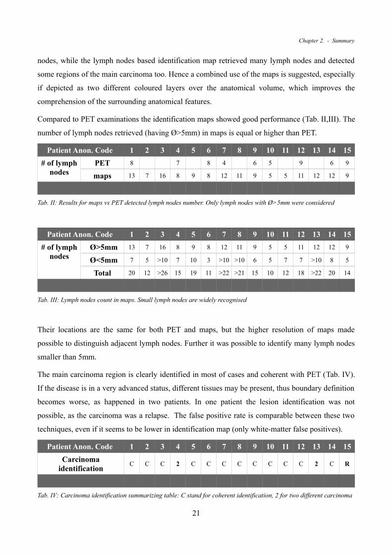
Compared to PET examinations the identification maps showed good performance (Tab. II,III). The
number of lymph nodes retrieved (having Ø>5mm) in maps is equal or higher than PET.
Patient Anon. Code 1 2 3 4 5 6 7 8 9 10 11 12 13 14 15
# of lymph nodes
PET 8 7 8 4 6 5 9 6 9
maps 13 7 16 8 9 8 12 11 9 5 5 11 12 12 9
Tab. II: Results for maps vs PET detected lymph nodes number. Only lymph nodes with Ø>5mm were considered
Patient Anon. Code 1 2 3 4 5 6 7 8 9 10 11 12 13 14 15
# of lymph nodes
Ø>5mm 13 7 16 8 9 8 12 11 9 5 5 11 12 12 9
Ø<5mm 7 5 >10 7 10 3 >10 >10 6 5 7 7 >10 8 5
Total 20 12 >26 15 19 11 >22 >21 15 10 12 18 >22 20 14
Tab. III: Lymph nodes count in maps. Small lymph nodes are widely recognised
Their locations are the same for both PET and maps, but the higher resolution of maps made
possible to distinguish adjacent lymph nodes. Further it was possible to identify many lymph nodes
smaller than 5mm.
The main carcinoma region is clearly identified in most of cases and coherent with PET (Tab. IV).
If the disease is in a very advanced status, different tissues may be present, thus boundary definition
becomes worse, as happened in two patients. In one patient the lesion identification was not
possible, as the carcinoma was a relapse. The false positive rate is comparable between these two
techniques, even if it seems to be lower in identification map (only white-matter false positives).
Patient Anon. Code 1 2 3 4 5 6 7 8 9 10 11 12 13 14 15
Carcinoma identification
C C C 2 C C C C C C C C 2 C R
Tab. IV: Carcinoma identification summarizing table: C stand for coherent identification, 2 for two different carcinoma
21

Quantitative Characterization and Identification of Lymph Nodes and Nasopharingeal Carcinoma by Coregistered MR Images
tissues with poor identification, R for relapse with non defined carcinoma boundaries and extended false positives.
These preliminary results suggest that this characterization map can play a diagnostic or prognostic
role similar to PET, improving the detail of the examination, in particular the number of lymph node
detected.
Conclusion
This study shows how a MR examination composed with different contrast images (T1,T2,T1-Gd
and DWI) can collect many informations about the pathological course of NPC. The technique
proposed in this study introduces tissue characterization maps, which could be a new tool in NPC
tissue identification and/or evaluation. The maps can be used as an identification tool especially
where the structures of interest are small or their dimensions are diminish with therapy. Furthermore
they can be a starting point for the segmentation of interest areas and calculation of quantitative
parameters (volume, mean ADC etc.).
The advantages of this technique are several: patient does not suffer ionizing radiation exposure, the
whole examination is taken in the same place, the MRI costs are very lower than PET, the
resolution of the resulting images is very higher. However results are preliminary and a clinical
validation of the work is needed to give a quantitative index of the reliability of this technique.
Finally an optimization work should be performed to improve calculation times, which is still too
high (more than two hours per examination session).
22

Chapter 2. - Summary
23

24

3.Sommario
Introduzione
Il carcinoma della rinofaringe (NPC) è un carcinoma a cellule squamose che si sviluppa
solitamente attorno all'imbocco della tromba d'Eustachio, nella parete laterale della rinofaringe.
Come in altri tumori, la prognosi del NPC si basa sulle dimensioni della lesione tumorale, sul
coinvolgimento dei linfonodi e sulla presenza di metastasi distanti. Per ottenere questa valutazione
solitamente vengono impiegate immagini di CT e PET, in grado individuare tessuti caratterizzati da
un elevato metabolismo. Inoltre un'indagine MR è necessaria per l'identificazione dell'anatomia dei
tessuti molli (mucosa) che circonda il carcinoma.
Recentemente la Diffusion Weighted MRI (DW-MRI o semplicemente DWI), una particolare tecnica
di MRI è in grado di creare immagini basate sulla mobilità dell'acqua nei tessuti è stata proposta
come una tecnica per la caratterizzazione del NPC. Un'elevata concentrazione del metabolita
identifica zone a metabolismo più elevato nella PET, ma anche la diffusione dell'acqua può essere
messa in relazione ad elevati interscambi cellulari, tipici di alcune lesioni oncologiche. Questo è
vero anche per il tumore principale del NPC e per i linfonodi patologici, facendo della DWI un utile
strumento per la caratterizzazione di queste strutture.
Osservando come un esperto radiologo sia in grado di identificare i tessuti patologici con un set di
immagini MR, formato da T1-Gd, T1, T2 e DWI, in questo studio abbiamo sviluppato un metodo
per caratterizzare i tessuti patologici del NPC basato sullo stesso set di immagini. Il processo
implementato è di tipo semiautomatico, richiedendo un intervento da parte del radiologo per la
localizzazione di campioni di tessuto. Quindi, dopo un'elaborazione basata su un approccio fuzzy,
siamo stati in grado di ottenere una mappa di caratterizzazione dei tessuti per ogni esame di ciascun
25

Quantitative Characterization and Identification of Lymph Nodes and Nasopharingeal Carcinoma by Coregistered MR Images
paziente, da valutare sovrapposta all'immagine anatomica T1-Gd. La mappa è stata confrontata con
immagini PET in modo da valutarne le prestazioni.
Metodi
Popolazione di Pazienti
Lo studio è stato condotto su 15 pazienti affetti da NPC, 3 donne e 12 uomini, di età compresa tra i
14 e i 60 anni al momento degli esami MR. Tutti i casi sono stati esaminati a diagnosi seguendo il
protocollo standard (descritto in seguito), in diverse sessioni d'esame. Il numero medio di sessioni
per paziente è tre, con un minimo di una ed un massimo di dieci, separate da un periodo di tempo
variabile da 3 a 12 mesi.
Il protocollo standard in questi casi clinici prevede l'acquisizione delle sequenze seguenti:
• T1 VIBE, per l'intero distretto testa-collo. Si tratta di una acquisizione 3D pesata T1 con
agente di contrasto Gadolinio, con risoluzione isotropica 0.65mm;RT=5.23ms, ET=2.05ms.
• T1 TSE per massiccio facciale e collo, acquisiti separatamente. Questa sequenza è una
Turbo Spin Echo pesata T1, con acquisizione di fette 2D a risoluzione planare di 0.65mm e
assiale di 4mm; RT=572ms; ET=12ms.
• T2 TSE per massiccio facciale e collo, acquisiti separatamente. Questa sequenza è una
Turbo Spin Echo pesata T2, con acquisizione di fette 2D a risoluzione planare di 0.5mm e
assiale di 4mm; RT=3180ms; ET=109ms.
• DWI, con b-values da 0 a 1000 (0,300,500,700,1000), acquisite separatamente per massiccio
facciale e collo. La sequenza è una DW EPI 2D con acquisizione assiale di fette 2D, con
risoluzione planare 2mm e assiale 5mm; RT=5200ms; ET=79ms.
Escludendo la T1 anatomica, le sequenze sono state acquisite tramite fette assiali in due volumi
separati, uno per il capo e uno per il collo. Per completare la diagnosi in 9 casi è stata acquisita
anche la PET.
Metodo di Registrazione
L'elaborazione delle immagini ha permesso di uniformare la risoluzione, la rappresentazione dei
distretti (testa e collo) e l'allineamento delle immagini, utilizzando l'immagine anatomica T1 VIBE
come riferimento. Questa modalità di acquisizione è infatti volumetrica, isotropica, composta da un
26

Chapter 3. - Sommario
unico volume che rappresenta entrambi i distretti testa e collo, e presenta la risoluzione più elevata
(0.6mm).
La prima operazione implementata è stata perciò il ricampionamento delle fette bidimensionali,
imponendo una griglia di campionamento 3D allineata alle coordinate paziente. La risoluzione
scelta è stata 0.5mm isotropica. La procedura è stata eseguita con una funzione Matlab
(TriScatteredInterp), che, basandosi su una triangolazione di Delone, permette di definire un
ricampionamento 3D dei dati con un'interpolazione lineare.
I volumi sono stati registrati seguendo i seguenti passaggi: 1) registrazioni rigide multirisoluzione
(correzione grossolana e fine delle differenze nella posizione del paziente), 2) fusione dei volumi
testa e collo, 3) trasformazione non rigida multirisoluzione (correzione dei movimenti del collo).
Tutte le registrazioni si sono basate sulla mutua informazione normalizzata (NMI), calcolata su 32
bin, e su una funzione di ottimizzazione basata sulla discesa del gradiente coniugato. La prima
registrazione è stata realizzata su un template T1 VIBE, sottoposto a un passabasso di tipo
gaussiano ( σ=2.5mm ), sottocampionato in successione a 5mm e 2.5mm, mentre la seconda
trasformazione rigida si è basata sul volume T1 VIBE nativo, con risoluzione di 1mm e quindi di
0.5mm. Per unire i volumi di testa e collo è stata utilizzata una media dei pixel non nulli, questo ha
permesso di evitare un oscuramento dei voxel sovrapposti. L'ultimo step è stato una registrazione
non rigida, realizzata su un template T1 VIBE sottoposto a blur gaussiano ( σ=3mm ), alle
risoluzioni di 5mm e 3mm. Nel calcolo dell'istogramma in quest'ultimo passaggio è stata imposta
una soglia di 50 per ridurre i tempi di calcolo, altrimenti proibitivi. I volumi DWI hanno la
peculiarità di essere già allineati al variare del b-value grazie alla modalità di acquisizione, perciò la
trasformazione è stata calcolata sull'immagine b0 ma applicata all'intero set DWI.
Mappe di caratterizzazione dei tessuti
Poiché introdurre un template definito a priori non è possibile, abbiamo riconosciuto i tessuti per
ogni paziente, grazie all'aiuto di un esperto radiologo. Poiché la lesione principale ed i linfonodi
hanno caratteristiche anatomiche diverse i due template sono stati raccolti con differenti modalità. Il
primo con un parallelepipedo da iscrivere nel tessuto del carcinoma. Il secondo è stato definito con
un cubo con lato di 9 voxel (4.5mm) completamente inscritto nella regione centrale di diversi
linfonodi (da 2 a 5). Queste ROI sono state utilizzate per raccogliere informazioni dalle 8 immagini
coregistrate (T1 VIBE, T1,T2 e le DWI per i b-value 0,300,500,700,1000).
27

Quantitative Characterization and Identification of Lymph Nodes and Nasopharingeal Carcinoma by Coregistered MR Images
La frequenza di occorrenza rappresentata negli istogrammi delle ROI può essere interpretata sia
come la composizione del campione di tessuto, sia come la probabilità che un voxel appartenga allo
stesso tessuto del campione. Un approccio statistico rigoroso richiederebbe l'uso del teorema di
Bayes, ma un approccio 8-dimensionale è decisamente troppo complesso. Perciò abbiamo
sviluppato un approccio di tipo fuzzy, che utilizza 8 distinte funzioni di appartenenza definite, dato
h jROIk , ovvero il numero di voxel con intensità k nella j-esima immagine, come segue:
M j I j x , y , z =h j
ROI I j x , y , z
maxkh j
ROIk
dove I jx , y , z è l'intensità del voxel di coordinate x , y , z nell'immagine j. Questa funzione
attibuisce valori di appartenenza più alti per voxel la cui intensità è vicina al massimo di h jROIk .
Allo stesso modo i punteggi più bassi corrispondono ai voxel con valori di intensità presenti con
meno frequenza all'interno della ROI, mentre i valori estranei sono associati a 0.
Avendo a disposizione 8 immagini, la mappa di identificazione grezza P x , y , z è stata ottenuta
come somma di ciascuna funzione di appartenenza, scalata tra 0 e 1000:
P x , y , z=∑j=1
8
M j I j x , y , z ⋅1000
8
Questa scelta da maggiore importanza alle immagini DWI (5 su 8 contributi) ed è giustificata
dall'importanza patofisiologica e diagnostica delle dinamiche di diffusione nella caratterizzazione di
tessuti. La mappa finale è stata ottenuta imponendo una soglia per eliminare i valori inferiori, meno
significativi:
P x , y , z={ P x , y , z P x , y , z th0 otherwise } ; th=250 .
Poiché i tessuti di interesse erano due, la procedura è stata applicata due volte, ottenendo una mappa
di identificazione basata sul campione della lesione e un'altra ricavata dal campione dei linfonodi.
Risultati
Registrazione
Per valutare l'allineamento delle immagini in una procedura di registrazione in letteratura è riportato
l'uso di due indici di similarità:
28

Chapter 3. - Sommario
NCC=∑p∈S
A p−AB p−B
∑p∈S
A p−A2∑p∈S
B p−B2
ovvero Normalized Cross Correlation (Cross Correlazione Normalizzata), dove p indica la
posizione mentre A e B sono i valori medi delle immagini corrispondenti; e la Normalized
Mutual Information (Mutua Informazione Normalizzata):
NMI A , B=H AH B
2 H A , B
dove H A è l'entropia dell'immagine A e H A , B è l'entropia congiunta delle due immagini.
Ad ogni step della registrazione (prima dell'allineamento (1), dopo la prima trasformazione rigida
(2), dopo la seconda trasformazione rigida (3) ed alla fine del processo (4)) abbiamo calcolato i
valori di NMI e NCC per tenere traccia delle performance della procedura. Entrambi gli indici sono
stati calcolati su una regione di sovrapposizione descritta da un cubo di lato 250 voxel collocato
29
Fig. III: Indici di similarità (valor medio ± deviazione standard) per i dati non elaborati (1), dopo la prima trasformazione rigida (2), la seconda trasformazione rigida (3) e la trasformazione non rigida (4). Nella riga superiore la NCC, in quella inferiore la NMI, mentre da destra a sinistra le statistiche per T1, T2 e DWI. L'andamento dei dati mostra il miglioramento dell'allineamento, considerando che le prestazioni della NCC sono limitate nel caso di registrazioni multimodali.

Quantitative Characterization and Identification of Lymph Nodes and Nasopharingeal Carcinoma by Coregistered MR Images
attorno al centro dell'immagine target. La NMI è stata calcolata su istogrammi e cross-istogrammi
da 128 bin (contro i 32 impiegati nella registrazione).
Come appare dai dati in figura (Fig. III), la NMI descrive un progressivo miglioramento della
registrazione, mentre la NCC ha un andamento molto più variegato. La differenza più importante è
il peggioramento del valore medio di NCC negli step 3 e 4 nella registrazione dei volumi T1 e T2.
Questo può essere dovuto al fatto che NMI e NCC si basano su differenti principi: mentre la NMI è
basata sul contenuto informativo la NCC è basata sull'intensità dei voxel. Gli indici di similarità
descrivono due incrementi principali in corrispondenza della prima trasformazione rigida e
dell'ultima non rigida. Lo step intermedio sembra essere meno rilevante poiché il suo allineamento è
più fine.
I risultati sono stati valutati dal punto di vista statistico con un t-test. La popolazione è stata
composta dagli indici di similarità raccolti prima e dopo lo step di registrazione, per ogni immagine.
L'ipotesi zero (che ci si aspetta venga rifiutata) è che gli indici allo step (n+1) ed allo step n seguano
due distribuzioni con la stessa media. Nella tabella (Tab. V) vengono riassunti i risultati del t-test,
riportando i P-value per ogni registrazione. Il test ha generalmente rifiutato l'ipotesi base, fatta
eccezione per due step della valutazione NCC.
Step RegistrazioneP-values
1-2 2-3 3-4
NMI
T1 P<0.0001 P<0.0001 P<0.0001
T2 P<0.0001 P<0.0001 P<0.0001
DWI P<0.0001 P<0.0001 P<0.0001
1-2 2-3 3-4
NCC
T1 P<0.0001 NS P<0.0001
T2 NS P<0.0001 P<0.01
DWI P<0.0001 P<0.0001 P<0.0001
Tab. V: Risultati del t-test e P-values corrispondenti. L'ipotesi è stata sempre confutata per tutti gli step della NMI, due step NCC hanno dimostrato P-values non significativi (celle grigie). Il risultato poco soddisfacente della NCC può essere messo in relazione con le limitazioni di questo indice di similarità in caso di registrazioni multimodali.
Mappe di caratterizzazione e confronto con PET
Le due mappe hanno mostrato un comportamento complementare: quella basata sul campione del
carcinoma riporta chiaramente il carcinoma stesso, ma include anche il guscio esterno dei linfonodi
patologici, mentre la mappa basata sul tessuto linfonodale riconosce molti linfonodi, ma anche
30

Chapter 3. - Sommario
alcune zone del carcinoma principale. Perciò è consigliabile un uso combinato delle due mappe, in
modo particolare se rappresentate come due layer con differenti scale cromatiche sovrapposti al
volume anatomico, in modo da mostrare anche l'anatomia che circonda i tessuti di interesse.
Se confrontate con la PET le mappe di identificazione presentano delle buone capacità (Tab.
VI,VII). Nelle mappe ottenute il numero di linfonodi evidenziati (con Ø>5mm) è uguale o maggiore
rispetto alla PET. La loro posizione è la stessa, sia nelle mappe sia nella PET, ma la maggiore
risoluzione delle mappe rende possibile la distinzione di linfonodi adiacenti. Inoltre è possibile
identificare molti linfonodi sotto i 5mm.
Codice Paziente Anon. 1 2 3 4 5 6 7 8 9 10 11 12 13 14 15
# di linfonodi
PET 8 7 8 4 6 5 9 6 9
mappe 13 7 16 8 9 8 12 11 9 5 5 11 12 12 9
Tab. VI: Risultati del confronto tra mappe e PET come numero di linfonodi riconosciuti. Solo i linfonodi con Ø>5mm sono stati considerati.
Codice Paziente Anon. 1 2 3 4 5 6 7 8 9 10 11 12 13 14 15
# di linfonodi
Ø>5mm 13 7 16 8 9 8 12 11 9 5 5 11 12 12 9
Ø<5mm 7 5 >10 7 10 3 >10 >10 6 5 7 7 >10 8 5
Totale 20 12 >26 15 19 11 >22 >21 15 10 12 18 >22 20 14
Tab. VII: Conteggio complessivo dei linfonodi nelle mappe. Anche linfonodi di dimensioni inferiori ai 5mm sono ampiamente e chiaramente riconosciuti.
31
Fig. IV: Mappe di caratterizzazione rappresentate sull'immagine anatomica T1 VIBE. I colori caldi rappresentano la mappa ottenuta dal campione del carcinoma, quelli freddi la mappa ottenuta con il campione linfonodale.

Quantitative Characterization and Identification of Lymph Nodes and Nasopharingeal Carcinoma by Coregistered MR Images
La regione del carcinoma principale è identificata quasi nella totalità dei casi ed è coerente con
l'immagine PET (Tab. VIII). Tuttavia se la malattia è in uno stadio particolarmente avanzato è
possibile che si presentino diversi tessuti tumorali, peggiorando la definizione dei bordi del
carcinoma stesso, come accaduto in due pazienti. In un caso clinico l'identificazione della lesione
non è stata possibile, poiché il carcinoma era un caso di “relapse” (ovvero una recidiva). La
presenza di falsi positivi nelle due metodologie è confrontabile, anche se apparentemente inferiore
nelle mappe (falsi positivi solamente nella materia bianca).
Codice Paziente Anon. 1 2 3 4 5 6 7 8 9 10 11 12 13 14 15
Identif. Carcinoma C C C 2 C C C C C C C C 2 C R
Tab. VIII: Tabella riassuntiva dell'identificazione del carcinoma: C=identificazione coerente; 2= due tessuti differenti, scarsa definizione mappa; R= caso di relapse (recidiva), falsi positivi e carcinoma non definito adeguatamente.
Questi risultati preliminari suggeriscono che questa mappa di caratterizzazione può rivestire un
ruolo diagnostico o prognostico simile a quello della PET, migliorando il dettaglio dell'esame, in
particolare il numero di linfonodi identificati.
Conclusioni
Questo studio mostra come un'analisi MR con differenti modalità di contrasto (T1, T2, T1-Gd e
DWI) possa raccogliere un gran numero di informazioni sullo stato di un NPC. La tecnica proposta
in questa ricerca potrebbe rappresentare un nuovo strumento per l'identificazione o la valutazione
dei tessuti nel NPC. Le mappe possono essere utilizzate come strumento di identificazione
specialmente laddove le dimensioni delle strutture anatomiche di interesse sono contenute o
vengono ridotte dalla terapia. Inoltre possono essere utilizzate come punto di partenza per una
segmentazione di aree di interesse e per il calcolo di parametri quantitativi (volume, ADC medio
etc.).
I vantaggi di questo metodo sono svariati: il paziente non è sottoposto a radiazioni ionizzanti, tutta
l'indagine è condotta sulla stessa macchina, i costi dell'esame MR sono molto inferiori rispetto alla
PET, la risoluzione delle immagini è molto migliore. In ogni caso è necessario una validazione
clinica che fornisca indici quantitativi riguardo l'affidabilità del metodo proposto. Infine un'ulteriore
ottimizzazione dell'algoritmo potrebbe migliorare i tempi di calcolo, ancora eccessivamente lunghi
(più di due ore per sessione d'esame).
32

Chapter 3. - Sommario
33

34

4.Introduction
The Nasopharingeal Carcinoma (NPC) is a squamous cell carcinoma that usually develops around
the ostium of the Eustachian tube in the lateral wall of the nasopharynx. Epidemiologic evidences
show that both environmental and genetic factors play roles in the development of NPC [1].
Standard treatment for NPC is radiotherapy, but concurrent adjuvant chemotherapy improves
survival rates. As with other cancers, the prognosis of NPC depends upon tumor size, lymph node
involvement, and distant metastasis (TMN staging). But NPC, in contrast to other head and neck
malignancies, is highly sensitive to radiation and chemotherapy [1].
Computed Tomography (CT) and Positron Emission Tomography (PET) images are usually
employed to obtain an accurate evaluation for radiotherapy or chemotherapy planning, giving
informations about tissues characterized by high metabolism such as carcinoma ones. These exams
are also performed during therapy to evaluate the disease course. Anyway a MR examination is
often necessary to correctly identify the anatomy of soft tissues (like mucosae) surrounding the
carcinoma.
Recently Diffusion Weighted MRI (DW-MRI or simply DWI), a particular MRI technique can
generate images based on water mobility in tissues, has been suggested as a potential technique for
NPC characterization. High metabolite concentration in PET identifies zones with higher
metabolism, but also water diffusion can be also related to higher cellular exchange, typical of some
oncological lesion [2]. This holds true for NPC main carcinoma and pathological lymph nodes,
making of DWI a useful tool to characterize those structures.
Frequently, in clinical practice, experienced physicians identify pathological tissues from the MR
image set, composed by an anatomic volumetric sequence with contrast medium (T1-Gd), T1 and
T2 contrasted images, and DWI. This happens mostly due to the low resolution of the PET imaging
35

Quantitative Characterization and Identification of Lymph Nodes and Nasopharingeal Carcinoma by Coregistered MR Images
technique, which is not enough to identify small structures such as lymph nodes smaller than 5mm.
Furthermore the patient undergoes just the MRI examinations, saving time and extra cost. Anyway
this procedure relies only on the experience of the clinician, who identifies the most interesting
structures, no quantitative characterization is usually performed.
This study developed a technique to improve the identification of carcinoma tissue and pathological
lymph nodes in cases of NPC, giving a quantitative characterization of the tissues. To this purpose
the method developed have been based on the same MR set of images evaluated in clinical practice
by the radiologist (T1-Gd, T1, T2 and DWI). The technique implemented is semi-automated, and,
once the template tissue is given, it emulates the radiologist decision making, defining a 3D tissue
characterization map.
The algorithm was applied to a population of 15 patient affected by NPC, 3 females and 12 males,
aged between 14 and 60, who underwent MRI at diagnosis and other successive examination
sessions. The original images were resampled and aligned, obtaining a fused set of images, with
high isotropic resolution (0.5mm). We identified two tissues templates at diagnosis, one for lymph
nodes and one for main carcinoma, with the aid of the physician. Hence we obtained a two maps,
that showed complementary tissues characterization. Thus they have been evaluated together, as
two differently coloured overlays of T1-Gd anatomical volume. The resulting map was compared
with PET to evaluate its performances.
36

Chapter 4. - Introduction
37

38

5.State of the Art
5.1 The Magnetic Resonance Imaging
Magnetic Resonance Imaging (MRI) is widely used as a diagnostic tool for its broad availability of
contrast modes, useful to represent living biological tissues. Just to mention some of them: proton
density; relaxation times; blood flow; blood oxygenation; tissue hardness; metabolite distribution
with chemical shift imaging. In common practice, these contrasts are manipulated to obtain
anatomical details or functional representation of tissue physiology. One of the main advantage is
surely the non-ionizing properties, respect to radiographic and PET (Positron Emission
Tomography) imaging. Although, to fully understand the features visible in MRI, it is important to
consider and comprehend the physics behind the different contrast modalities.
5.1.1 Physical principles
The Nuclear Magnetic Resonance (NMR) phenomenon in bulk matter was first demonstrated by
Bloch [3] and Purcell et Al. [4] in 1946. Since then, MR has developed into sophisticated technique
with application in a wide variety of disciplines that now include Physics, Chemistry, Biology and
Medicine. Over the years, MR has proved to be an invaluable tool for molecular structure
determination and investigation of molecular dynamics in solids and liquids. In its latest
development, application of MR to studies of living systems has attracted considerable attention
from biochemists and clinicians alike. The rapid progress to diverse fields of study can be attributed
to the development of pulse Fourier transform techniques in the late 1960's [5]. Additional impetus
39

Quantitative Characterization and Identification of Lymph Nodes and Nasopharingeal Carcinoma by Coregistered MR Images
was provided by the development of Fast Fourier Transform (FFT) algorithms, advances in
computer technology and the advent of high field super conductive magnets. Then, introduction of
new experimental concepts as two dimensional MR has further broadened its applications, bringing
to the Magnetic Resonance Imaging technique [6].
Even if the phenomenon itself is described by the quantum physic formalism, it is possible to
achieve an excellent comprehension of it by a classical mechanic approach (Bloch). In this
paragraphs we are going to employ this formalism, avoiding too complex notions which here cannot
be adequately treated. One of the fundamental concept in this formalization of the nuclear magnetic
resonance phenomenon is the spin, a measurable quantity of an atomic nucleus that describes some
of its movement properties. In classical terms we can consider the spin quantum I , which act as an
angular moment. In quantum mechanics we can introduce the spin quantum number I as the sum
of the unpaired I of each nucleon [7]. Usually nucleons are paired with anti-parallel spins: this
means that nuclei which has even number of nucleons have I=0 , making them useless for
magnetic resonance. Furthermore each I can be associated to 2 I1 energetic levels. The most
suitable nuclide for medical MRI is the Hydrogen 1H, for its abundance in the biological tissues and
for its physical properties which make its MR signal well detectable.
As these particles have an electric charge and they are spinning, a magnetic momentum µ is
generated. The link between magnetic and mechanic momentum comes in the equation:
=∗I
where the gyromagnetic ratio is a constant typical of each nuclide [7]. Given the quantum
mechanic theory =∣∣ can have a range of discrete values, as described by the form:
=h
2 I I1
where h is the Planck constant. This means that each single nucleus generate a small contribution
to the overall magnetization, which still is null, as each nuclear spin has a random orientation [7].
It's possible though to record an overall macroscopic magnetization by applying an external
magnetic field B0 . For our purpose let's suppose it is oriented along the z-axis of the coordinates
system. In that situation the component of µ along z results in:
z=m Ih
2
40

Chapter 5. - The Magnetic Resonance Imaging
where m I is the magnetic quantum number. That quantity is discrete, and depends directly on I ,
( m I=−I ,−I−1,... , I−1, I ), carrying information about the possible orientation of µ in an
external magnetic field B0 . Hydrogen nuclei (1H) have I=1/2 , thus the possible orientation are
two, parallel and anti-parallel. Components along other dimensions ( x and y ) are still random and
not known a priori.
Recalling again the classical physics formalism, any proton is subject of a mechanic momentum
× B0 , which can be known as:
d mud t
=× B0
this means the vector µ moves in a precession around the B0 direction, with an angular speed
described by the Larmor law:
=− B0
The presence of an external magnetic field imposes two orientation for spin axis. The configuration
anyway is not symmetrical: this is caused by a slight energetic gap between the two states, which
obviously creates a shift toward the more stable. This is described by the Boltzmann statistic
N ↑
N ↓
=expEK T
where
E=E↓−E↑=h
2B0
As comes from this equation the shift between the two states, and thus the overall magnetization, is
really small and the difference for a B0 field of 1 Tesla and 300K is just few protons per million.
Rather than the actual behaviour of the protons the aim of the measurement in the MRI is the
overall magnetization indeed: when an object is in a magnetic field B0 it generates an overall
magnetization M(Figure 1), proportional to the field itself and to the number of excited spins (and
thus to the proton density ).
41

Quantitative Characterization and Identification of Lymph Nodes and Nasopharingeal Carcinoma by Coregistered MR Images
To obtain a measure of the magnetization M it is necessary to perturb the static magnetic field with
another one, that rotates on a perpendicular plane. Further the non static field B1 must have the
same frequency of the precession motion: the Larmor frequency. This generates a resonance
phenomenon, called nuclear magnetic resonance: the electromagnetic radiation photons of the B1
field have energy:
h=h
2B0
which happens to be the same quantum that separates the parallel spin status from the antiparallel
one. Thus it happens that protons have the chance to move from one state to the other. Another
advantage of the hydrogen nuclide is that the Larmor frequency is between 1÷100 MHz which
means that the excitation field B1 is in the radio-frequency (RF) band, which does not have
ionizing properties, furthermore it can pass through the tissues without an appreciable attenuation.
As explained before the proton spin movement can be considered a precession around the B0
direction, thus, during the radio-frequency excitation, the orientation changes and the spin describes
a spiral, moving from the magnetic field alignment toward the perpendicular plane (Figure 2).
Therefore to define the flip angle term we need to move the observation point to the rotating field
B1 : when looking at the spin movement with a coordinates system that rotates following B1 the
excitation effect is a change in the angle described by the flip and the B0 direction, the flip angle.
42
Figure 1: Magnetization vector and spins orientation due to an external field B0 . This
behaviour can be examined as a precession motion in classical physics. Adapted from [7].

Chapter 5. - The Magnetic Resonance Imaging
Assuming a step impulse the flip angle can be evaluated as:
= t= B1 t
where t is the application time of the excitation radio-frequency (rotating field B1 ) [7]. If the
impulse time is long enough to produce a rotation of /2 it is called 90° impulse, in the same
way if = we have a 180° impulse. When the spin orientation has a component in the plane
perpendicular to the B0 direction it is possible to detect a transversal component of M :
M 0sin exp [ j t fi ]
which generates a current in the receiving coil. If is exactly the spin orientation is simply
inverted and there is still no transversal magnetization. Once the radio-frequency excitation ends the
system decays in the initial status: the longitudinal component (respect to the z axis) recovers its
original value, and the transversal one disappears.
5.1.2 MR signal: the Free Induction Decay
Once displaced from the z axis by the RF pulse the net magnetization M is no longer at
equilibrium. We denoted this non equilibrium magnetization vector with M , and the magnitudes of
its component along the x , y and z axis will we denoted by M x , M y and M z respectively.
43
Figure 2: The spin orientation during the RF excitation. a) Observation with coordinates rotating with B1 ; b) Absolute coordinates view. The movement described is clearly a spiral in b), but in a) it can be
described by a simple planar angle .Adapted from [7]

Quantitative Characterization and Identification of Lymph Nodes and Nasopharingeal Carcinoma by Coregistered MR Images
The magnitude of the component of in M the transverse x-y plane (i.e. the resultant of M x and
M y ) will be denoted as M xy . The equilibrium magnetization vector M 0 represents the situation
in which M is aligned along the z axis corresponding to the case of M z=M 0 and M xy=0 .
It can be shown that the amplitude of the alternating voltage induced in the receiver coil is
proportional to the transverse magnetization component M xy . Hence, a maximum amplitude
voltage signal is obtained following a /2 pulse since such pulse creates the maximum M xy
component, equal to M 0 . In general, for RF pulse of flip angle the amplitude of the alternating
voltage is proportional to M 0sin .
As a result of relaxation M xy (i.e. the amplitudes of oscillation of M x and M y ) decays to zero
exponentially; thus the voltage signal observed in practice corresponds to an oscillating signal at the
Larmor frequency, with exponentially decaying signal amplitude. This type of decaying signal,
obtained in the absence of B1 is called Free Induction Decay (FID).
5.1.3 Spin Relaxation dynamics
Having excited the nuclei in order to flip them towards the transverse plane they begin the relax
back to their equilibrium position as soon as the RF pulse is switched off. There are two main
features of the relaxation: a dephasing of the spins (whose phase were coherent during the RF
excitation), and a realignment along the z axis as they loose the energy absorbed from the RF
pulse. In the classical vector model, this corresponds to the return of the magnetization M to the
equilibrium position aligned along z . Thus, during the relaxation period, any transverse
magnetization component M xy created by the RF pulse decays to zero, and, at the same time the
44
Figure 3: After a 90° RF pulse, the longitudinal component of magnetization is null as spin vectors loose coherence rapidly. From left to right it is shown the recovery process of longitudinal magnetization.

Chapter 5. - The Magnetic Resonance Imaging
longitudinal magnetization component M z , recovers to the equilibrium value of M 0 . The decay of
M xy and the recovery of M z are two distinct processes.
The more intuitive process that leads to the recovery of equilibrium magnetization is the loss of
energy of the spins. That energy, in fact, was given to the nuclei by the RF and it made possible the
change of spin orientation: after the RF excitation, if there was no energy loss, the magnetization
would be persistent. What happens actually is that the nuclei interact with the surrounding medium
(called lattice) loosing energy. This tend to make the magnetization vector return from the
perpendicular plane to the original orientation (parallel to B0 direction), causing a decay of the
transversal component M xy in favour of the longitudinal component M z (Figure 3). This action is
called spin-lattice relaxation, and, after an degree pulse it can be described by:
M z t =M 01−1−cos e
−tT 1
T 1 is called spin-lattice relaxation time.
If two nuclei come close together, each of them experiences a slight difference in magnetic field, as
the magnetic moment of the other protons adds or subtracts from the main field. Consequently their
precessional frequencies change slightly respect to the overall Larmor frequency. This happens for
thousands of spin couples and it is irreversible, so the dephasing angle increases until the overall
coherence is fully disrupted (Figure 4).
This phenomenon is called spin-spin relaxation and, in contrast with what happens due to spin-
lattice relaxation, the transversal magnetization decreases without a recovery in longitudinal
component.
45
Figure 4: After a 90° RF pulse the magnetization moves to the transversal plane. There the spins start to interact and thus they loose coherence, resulting in magnetization decay.

Quantitative Characterization and Identification of Lymph Nodes and Nasopharingeal Carcinoma by Coregistered MR Images
This decaying, which follows an degree pulse can be described with the equation:
M xy t =M 0 sin⋅e i 0 t⋅e−t
T2
where T 2 is the spin-spin relaxation time.
T 1 and T 2 are determined by the molecular environment, thus they depend on and can describe the
composition of the sample or biological tissue. For pure liquids T 1 = T 2 , while for biological
tissues T 1 > T 2 . Further, as we will describe later, the magnetization field B0 is non ideal, both for
imperfections in the superconductor coil and for the spatial coding gradient. This interferes in the
theoretic behaviour, mimicking the decay of transverse magnetization caused by relaxation and
hence accelerating the process of decay. To describe this phenomenon it is commonly used a
different time constant T 2* :
1
T 2*=
1T 2
1
T 2 '
where T 2 ' describes the decay proportionally to the field inhomogeneity extent B0 :
1T 2 '
=B0
Another parameter useful to characterize the samples is the density of the active (in our case 1H)
nuclides. Hence the involved nuclei are simple protons it is commonly referred as proton density,
defined . This measure is closely related to the water presence (which has the most content of
protons) in biological tissues, so high water content (liver, blood), means high proton density, while
low water content (bone, air).
We can summarize the behaviour of the magnetization M and thus the overall behaviour of the
nuclides, when B0 is aligned to the z axis, with the Bloch equation [7]:
d M t d t
= M t ×Bt – R M t – M 0
where B t = B0 B1t and M 0 is the magnetization due to B0 . The relaxation matrix R is
composed by the terms that describe the decay of the magnetization and thus depends on the time
constants T 1 and T 2 . In the condition we are studying it can be written simply as a diagonal
46

Chapter 5. - The Magnetic Resonance Imaging
matrix, where one term defines the longitudinal decay and the other the transversal damping [7],
while M 0 has just one not-null component along the z axis:
R=[1/T 1 0 0
0 1/T 2 00 0 1/T 2
] ; M 0=[ 0 0 M 0 ]
5.1.4 Imaging sequences and encoding principles
Considering these properties of the magnetization, several pulse sequences can generate a particular
magnetization vector, with custom orientation or decay. The aim of these procedures is to evidence
the dependence of the FID on one of the time constants ( T 1 , T 2 ) or its dependence on the proton
density. We denote a coordinates system whose transverse plane is rotating at angular frequency
, defined by x ' , y ' , z ' .
This can be described mathematically as:
{x '=cos t x−sin t yy '=sin t xcos t y
z '=z }In the following paragraphs we will discuss briefly the pulse sequences commonly used to generate
MR images.
Inversion Recovery pulse
In the Inversion Recovery (IR) pulse the equilibrium
magnetization M 0 is initially perturbed by a 180° pulse.
After a time period TI (Time of Inversion), a second
perturbation is given as a 90° pulse (Figure 5). Assuming
the RF pulses are applied along the x ' axis, the 180°
pulse cause the magnetization to rotate by 180° about x '
axis, and at the end of it, will be oriented along the
negative z axis.
47
Figure 5: Inversion Recovery pulse sequence. The first pulse is a 180° RF is followed by a 90° pulse. This generates the FID.

Quantitative Characterization and Identification of Lymph Nodes and Nasopharingeal Carcinoma by Coregistered MR Images
During the TI period the magnetization relaxes and its value is:
M z=M 0[1– 2e
−TIT 1]
The application of a 90° pulse causes the magnetization present at that time to rotate by 90° about
the x ' axis, thus at the end of the pulse the magnetization will be directed along the y ' axis. In the
following instances a FID will be observed: its initial amplitude will be proportional to the M z at
the end of the time period TI.
Gradient Echo pulse
The Gradient Echo pulse (GE) includes an degree
pulse followed by a time varying gradient magnetic field
to generate an echo rather than a FID signal. It relies on
the concept that a gradient field can dephase and then
rephase a signal in a controlled way, so that one or more
echo signals can be generated.
After the excitation with the degrees RF pulse, a
negative gradient is switched on. If it is oriented along the
x axis, the spins in that direction will precede at different
Larmor frequencies, thus will acquire different phases
described by:
x , t =∫0
t− x
G x d =− xG x t
hence coherence becomes lower as time passes. When the
spins are completely dephased an inverted magnetic gradient is turned on, with the same strength of
the first gradient. This will cause spins to invert the dephasing direction and thus the transverse
magnetization gains coherence: the signal perceived re-grows (Figure 6). Their phases are now
described by:
x , t =− x G x t '∫t '
t
x G x d
The time necessary for spins to rephase is called TE (Time of Echo).
48
Figure 6: Gredient Echo pulse sequence. The gradient inversion generates an echo which decay follows spin-spin relaxation time constant.

Chapter 5. - The Magnetic Resonance Imaging
Spin Echo pulse
This pulse sequence is similar to the inversion recovery,
but the procedure of the excitation RF is inverted. In fact
the first pulse is a 90° (about the x ' axis) pulse that
rotates the magnetization, aligning it to the y ' axis
(Figure 7). Once the excitation ended, the magnetization
tends to decay due to loss of coherence between spins.
Their movement continues till the 180° (about the x '
axis) pulse is given at TE/2: its effect is to invert the spin
precession direction.
Hence, supposing that the precession speed does not
change during TE, this means that all the components
will return aligned to the y ' axis in the same instant,
generating an echo signal. The net magnetization at that time is determined by the spin-spin
relaxation only, being described as:
M y=M 0 e−TE
T2
Note that this equation is applicable just when the effects of diffusion or perfusion are negligible in
the samples: movement of the nuclei during the TE time causes the echo amplitude to be reduced.
Spatial encoding and k-space
To identify the MR signal in a tridimensional space it is necessary to apply three different magnetic
gradients:
B z x=B0 xG x ; G x=∂B z
∂ xG y=
∂ B z
∂ yG z=
∂ B z
∂ z
This procedure makes possible to change selectively the Larmor frequency so that only interest
nuclides give signal, so, hypothesizing a gradient along x axis:
x =B0x G x
Thus in the resulting signal there will be differently phased FID with different frequencies:
separating them with a little processing makes possible to identify the source of each of them. The
three steps are called slice selection, frequency encoding and phase encoding.
49
Figure 7: Spin Echo pulse sequence. In this sequence the echo is generated with a 180° pulse, which inverts the spin precession.

Quantitative Characterization and Identification of Lymph Nodes and Nasopharingeal Carcinoma by Coregistered MR Images
For what concerns slice selection, both a gradient (slice selecting) and a specially designed RF pulse
are applied: the gradient is perpendicular to the desired slice, so that the RF excitation is limited to
a chosen slice within the sample. Hence if we want to image a slice in the xy-plane, we have to
apply a gradient along the z axis and choose the pulse frequency so that:
z = B z z =B0zG z
The pulse, anyway, is not an on-off step, but has a modulation so that it contains a bandwidth,
thus the slice thickness is:
z=
G z
is related to the shape and the duration of the pulse and it is the full width at half maximum
(FWHM) of pulse frequency spectrum. The slice profile is determined by the spectral content of the
selective pulse, and it is approximately reconstructible by the Fourier Transform of the RF pulse
envelope.
Frequency encoding consist on the activation of a gradient during the MR signal acquisition. Let's
consider an ideal linear object aligned along x with spin density x , which already underwent a
pulse to move the magnetization on the transverse plane, and whose spins are already preceding
with speed 0 before the gradient is imposed. Defining the gradient as xG x , the precession
frequency at position x is:
x , t =0 xG x t
In the same way the FID signal ds x , t , ignoring the transverse relaxation effect is:
ds x , t =C x dxe−iBo xG x t
where C depends on the flip angle, the main field strength, etc. The signal received from the entire
sample is:
s t=∫−∞
∞
ds x , t =∫−∞
∞
C xe−i B0 xG x t dx=[∫−∞
∞
C x e−i xG x t dx] e−i0 t
Demodulating the frequency, given G freq=G x ,G y ,G z the received FID is given by:
s t=C∫−∞
∞
r e−iG freq t dr
50

Chapter 5. - The Magnetic Resonance Imaging
In presence of a magnetic gradient G y , we are able to introduce a phase encoding, as the overall
magnetic field at the location y is B y =B0 yG y , the resonance frequency will be:
y=B z y=B0 yG y
causing a shift of y = yG y . As a result, the nuclei precess at different rates according to their
position. Hence the phase shift at location y and time t is given by:
y , t = yG y t
The presence of the gradient introduces a phase shift that persist during the following time, and it
can be retrieved in the acquired signal. If we turn on a gradient for a short interval t y the local
signal under influence will be:
ds y , t ={ y e−iB0 y G y t 0≤t≤t y
y e−iB0 t y G y t y t≥t y
}where y is the proton density along y.
Since the phase shift is related to the signal location by linear equation the signal is said to be phase
encoded. Phase encoding along arbitrary direction can be also done for multidimensional object by
turning on G x , G y , G z simultaneously during the phase-encoding period G phas=G x ,G y ,G z for
0≤t≤t y ; the initial angle is r =−r G phas t y . Similarly to frequency encoding, the signal
received is the sum of the differently phase shifted contributes:
s t=∫−∞
∞
ds r , t =C [∫−∞
∞
r e−iG phas tG dr ]e−i0 t
where the sinusoidal behaviour can be removed with demodulation.
Defining the phase encoding step, denoted with p, as a gradient amplitude multiplier such as
G y' = pG y , we can introduce a different phase encoding step for varying the amplitude of each
phase encoding gradient. Thus the sequence of phase shifts added to a magnetization vector at the
location r 0 as p y0=− r0 p G p tG . Therefore the expression for a set of different encoding can
be written as:
s pt =C [∫
−∞
∞
r e−i p r Gr tG dy ]e−i0 t
51

Quantitative Characterization and Identification of Lymph Nodes and Nasopharingeal Carcinoma by Coregistered MR Images
A Fourier Transform can be used again to compute the position of the object in the y direction if
applied to the sequence s pt for different p-values.
If P frequency encoded MR signals are obtained along the x-axis, each one with a different value of
phase encoding gradient amplitude along the y-axis:
s pt =C [∫
−∞
∞
∫−∞
∞
x , y e−i xG xt ypG y t Gdx dy ]e−i0 t
In a such way, k-space data are sampled data, memorized in a matrix of F×P , if F is the number
of samples along reading gradient and P the number of times the phase gradient is activated.
Then, if each MR signal is sampled and t is the time interval and we consider the demodulated
signal, so we can obtain:
{s f , p=C ∫
−∞
∞
∫−∞
∞
x , y e−ixG x f t ypG y t Gdx dy
0≤ f ≤F
−P / 2≤ p≤P /2}
To synthesize we can write:
s k x , k y=C∫−∞
∞
∫−∞
∞
x , ye−i xk x yk ydx dy ; where {k x= f t G x
k y= p t y G y}
this shows that the data matrix s k x , k y is a sampling of the Fourier coefficients of the function
x , y . Therefore, by applying a two dimensional inverse Fourier Transform to s f , p , the
result will be an estimate of the function x , y . So that a more general form is:
{sk t = ∫
sample
r ,v e−2 I k t−r d r
k t =∫0
t
G d }where r ,v is a function of position r and v where v is a vector of parameters
v=[r ,T 1r , T 2r ...TR ,TE , , ...] that describes the dependence on tissue parameters ( ,
T 1 , T 2 , etc.) and scanner parameters (TR, TE, etc.)
52

Chapter 5. - The Magnetic Resonance Imaging
k-space trajectories for fast acquisition
The 2-D FT method is excellent for generating high resolution images, but its acquisition time is
slow, since it defines a row of k-space coefficients for each TR. There are other methods to acquire
images faster, one of them is the echo-planar imaging (EPI) method, but usually the counterpart of
the acquisition time reduction is a loss in image resolution. The EPI pulse sequence is characterized
by a “zig-zag”-like acquisition trajectory, that goes rapidly in the frequency direction ( k x ) and
moves in small steps in the phase direction ( k y ). EPI can be spin-echo or gradient-echo based,
which will result respectively in a T 2 or a T 2* weighted image. This means to acquire several
echoes for every RF, each defining a row in the k-space.
Usually this approach is a so called single-shot imaging method, since it needs just a single RF
pulse to obtain the whole slice data. This is true for the simplest approach, which can give just a
modest spatial resolution. To improve that the k-space can be split in 2, 4 or 8 parts, each of them
acquired with a RF pulse. This will give a compromise augmenting resolution, but renouncing to
the snapshot ability to freeze physiological motion [8].
Similar in concept to EPI, is Turbo Spin Echo (TSE) in which multiple 180° RF pulses are used to
continually refocus the decaying M xy magnetization. This makes possible to generate several
echoes for each 90° RF, introducing a phase encoding gradient specific for each echo. In this way
multiple rows are acquired in the k-space, one for each 180° pulse.
5.1.5 Diffusion-Weighted Imaging
When we were discussing about the spin echo pulse sequence we noticed that the equation validity
was related to the entity of diffusion and perfusion in biological samples. It happens, in fact, that the
movement of spins can introduce some difference in their relaxation behaviour due to their speed
and position changing. In the following paragraph we will introduce how this behaviour changing
can lead to a specific contrast technique to create Diffusion Weighted (DW) images.
Basic diffusion concepts
The random movement of particles suspended in a fluid is called Brownian motion in honour of the
botanist who first described it. A detailed framework of the Brownian motion was published by
Albert Einstein in 1905.
53

Quantitative Characterization and Identification of Lymph Nodes and Nasopharingeal Carcinoma by Coregistered MR Images
The following relationship is a good starting point [9]:
⟨r2⟩=6 D t
where the first term represents the squared displacement of a particle allowed to diffuse freely in
three dimensions during the time interval t , and D is the diffusion coefficient which represents
the dependence of this phenomenon on temperature and media viscosity. When diffusive particles
and the media are the same D is also referred to as the self-diffusion coefficient. Let's consider, for
example, pure water at body temperature which is known to have D=3×10⁻³ mm2 s−1 . Their root
mean square (rms) displacement over an interval t=50ms is given by the last equation and yields
to 30×10−3 mm=30m [2]. If we compare that displacement to the size of the cell, which usually
is of several microns, it is clear that the probability that water molecules encounter many cellular
and subcellular impediments during the 50 ms period is high. Extracellular water will also
encounter impediments due to the tortuosity of the extracellular paths in dense tissues [10]. In
simple solutions of large-particle solute in small molecule solvent, the diffusion coefficient of the
large particle is inversely related to the particle size R according to the Stokes-Einstein equation:
D solute=TR
where combines the fundamental constants, media viscosity and solute surface properties; while
T is the absolute temperature. This actually means that the water mobility is reduced due to the
presence of macro molecules, and, as we will see, the water mobility reduction, relatively to free
diffusion, will be used as prove of the non-water tissue constituents presence and behaviour.
The time-dependence of rms displacement of diffusing molecules suggests one may use time as a
variable to probe cellular distance scales in tissues. This is usually not adopted as it is difficult to
achieve a sufficient sensitivity to diffusion effects at very short time intervals when using a human
MR imaging equipment.
Magnetic resonance measurement of diffusion
Similarly of what we said it happens during the gradient-echo pulse in the previous section, we can
define a phase shift for a molecule migrating along a trajectory r t in a gradient field as:
t=−∫0
t
G ⋅r d
54

Chapter 5. - The Magnetic Resonance Imaging
For the scenario of many spins having random directions it is reasonable to expect there is an equal
number of positive and negative phase shifts, giving a null overall shifting, while a coherent
diffusive path leads to a detectable shifting.
Looking at the last equation it can be clearly derived that a larger phase shift can be obtained by
augmenting the integral interval, the path length, the gradient duration and/or gradient field
strength. This general line of logic can be applied to the Bloch equation, modifying it to include
spin diffusion. So it is possible to denote the attenuation of spin diffusion by the Bloch-Torrey
equation [11]:
S t =S 0 e−D∫
0
t
c ⋅cd
where S is the diffusion attenuated signal, S0 is the non attenuated signal, D is the spin diffusion
coefficient and c t relates to the time integral given by:
c t =∫0
t
G d
Creating a particular spin echo sequence, called often Stejskal-Tanner pulse field gradient (PFG)
[12], it is possible to enhance the diffusive dependence of the phase shift. The sequence resembles a
spin-echo pulse, in which RF are interleaved by gradients (Figure 8). In these condition it is
possible to define the b-value concept [13], as:
b=∫0
TE
c ⋅c d =G2[ –
3]
Frequently, only the gradient amplitude is changed to vary the b-value in a diffusion imaging
sequence.
55
Figure 8: Standard pulse field gradient waveform for diffusion sensitization. The sequence is very similar to conventional spin-echo

Quantitative Characterization and Identification of Lymph Nodes and Nasopharingeal Carcinoma by Coregistered MR Images
This leads to a change in signal as a function of b-value, from which the diffusion can be obtained
with at least a couple of measurements [2]:
D=1
b2 – b1
ln [ S b1
S b2 ]Often one of the PFG gradients has no amplitude, while more than two b-values images are
acquired to furnish a more accurate estimation of the coefficient, derived by a linear fit of ln [S b]
versus b-value.
Anisotropic diffusion
The formalism analysed in the previous paragraphs only considers isotropic molecular diffusion,
which is to say there is no directional dependence on how the molecules migrate. Anyway, even if
most non-neuro tissues show nearly isotropic water diffusion, one should not assume tissues are
isotropic when performing quantitative diffusion imaging experiments.
To allow anisotropy while avoiding several complex mathematical issues we shall simply state that
anisotropic systems can be described by a 3×3 second-order rank diffusion tensor [14]:
D=[D xx D xy D xz
D yx D yy D yz
D zx Dzy D zz]
Moreover we can generalize the other equations:
b lm=2∫
0
TTE
∫0
G l ' d ' ⋅∫0
Gm ' d ' d ; ln S 0
S b=∑
l=1
3
∑m=1
3
blm Dlm
where l and m relate to any of the three gradient direction [ x , y , z ] . The b lm elements of the b-
matrix are the anisotropic corollary to the isotropic b-factor and are calculated for each gradient
condition of a directionally sensitive diffusion acquisition. The diffusion tensor is symmetric [2]
thus it contains six unique values. Hence to determine its matrix is necessary to describe at least six
non-colinear diffusion gradient directions (plus b=0). Although a scalar invariant quantity are highly
desirable as their value is independent of relative diffusion orientation in tissues: that is the main
motivation behind the wide use of mean diffusivity Dave [14].
56

Chapter 5. - The Magnetic Resonance Imaging
Furthermore Dave can be obtained just with three diffusion measurements along the orthogonal
axes:
Dave=D xxD yyD zz
3
Diffusion measurements in vivo
In living tissues there are physiologic motions unrelated to diffusion that can mimic diffusion
processes and introduce errors in measurements. For instance we can consider the blood flow, the
respiratory and cardiac motions. A way to reduce movements effect is to diminish the acquisition
time: the most clinically successful DW approaches are based on single shot EPI, even if it is non
immune to motion artefacts [2].
Thus far, our mathematical description denotes molecular mobility by simple diffusion coefficients
D, Dlm and Dave ; although water motion through cellular tissues is highly complex. Perfusion and
other bulk tissue motions further complicate the in vivo situation: the result is that diffusion
measurements of tissues are qualified as apparent diffusion coefficient (ADC). To remember these
issues is commonly used the ADC term [2], while the use of this constant is the same of the D or
Dave .
Lower and higher b-value estimation errors
As said before one of the most important thing to understand is the presence of an inextricable
linking between diffusion and perfusion. Especially at low b-values ( b≤100 s/mm2 ) the perfusion
fraction is dominant [8]. To avoid ADC overestimation in that range it is common to employ higher
b-values and to implement the fitting on more than two b-values. On the other hand at very high b-
values (over 1000 s/mm2 ) the SNR is not reasonable [2], so measurements over that value are non
advisable.
Simulation can isolate the impact of both this phenomenon since the effects of each can be
controlled independently by the programmer. It also provides guidance to design protocols for
accurate ADC estimations [15]. To summarize the results, perfusion tends to inflate ADC estimates,
while too high b-values causes underestimation, as the log curve tends to flatten and follow the
noise floor.
57

Quantitative Characterization and Identification of Lymph Nodes and Nasopharingeal Carcinoma by Coregistered MR Images
Thus the most common way to avoid these issues is to acquire only few b-values in the best range,
so it is possible to characterize the tissue with an acceptable SNR and without overestimations
caused by perfusion [2]. Other approaches might also be used, but their results are often more
effort-taking to obtain than useful.
58

Chapter 5. - Biomedical Images Registration
5.2 Biomedical Images Registration
In the biomedical imaging environment the clinical practice is definitively moving from analogical
imaging techniques and radiographic films to computerized approaches. The potential benefits that
lays behind these approaches are many, but a particular attention should be paid to the possibility of
accurately aligning the information in different images, and providing tools for visualizing the
combined images. A critical stage in this process is indeed the alignment (or registration) of the
images. There are many surveys of the medical image registration literature (e.g. Maurer and
Fitzpatrick 1993, van den Elsen et al 1993, Maintz and Viergever 1998, Derek L G Hill, Philipp G
et al 2000). This provides a large amount of informations on the argument; in this chapter we focus
the discussion on some of the most widely used registration algorithms rather than providing a
comprehensive survey of all the literature in this field. A particular attention will be given to the
algorithm by Reuckert, Sonoda et al [16], implemented in the IRTK software suite, which has been
used in this study.
5.2.1 The registration problem
With the term “registration” we mean “the spatial alignment between images of the same (or
different) subjects, acquired with the same (or different) modalities, and also the registration of
images with the coordinate system of a treatment device or tracked localizer” [17]. The
transformation itself includes both the transformation that aligns the intensity values and the
resampling needed to achieve the final result of discrete images (2D or 3D).
Denoting the spatial transformation with T, mapping the coordinates from the floating image I f to
reference image I r , we can write:
T : I f I r⇔T I f = I r
The domain of T is defined as the search space of the registration, while the function that defines
the quality of the alignment is called similarity metric[8]. An optimization algorithm (usually called
search strategy) is used to calculate the transformation that optimizes the similarity function
(Figure 9).
59
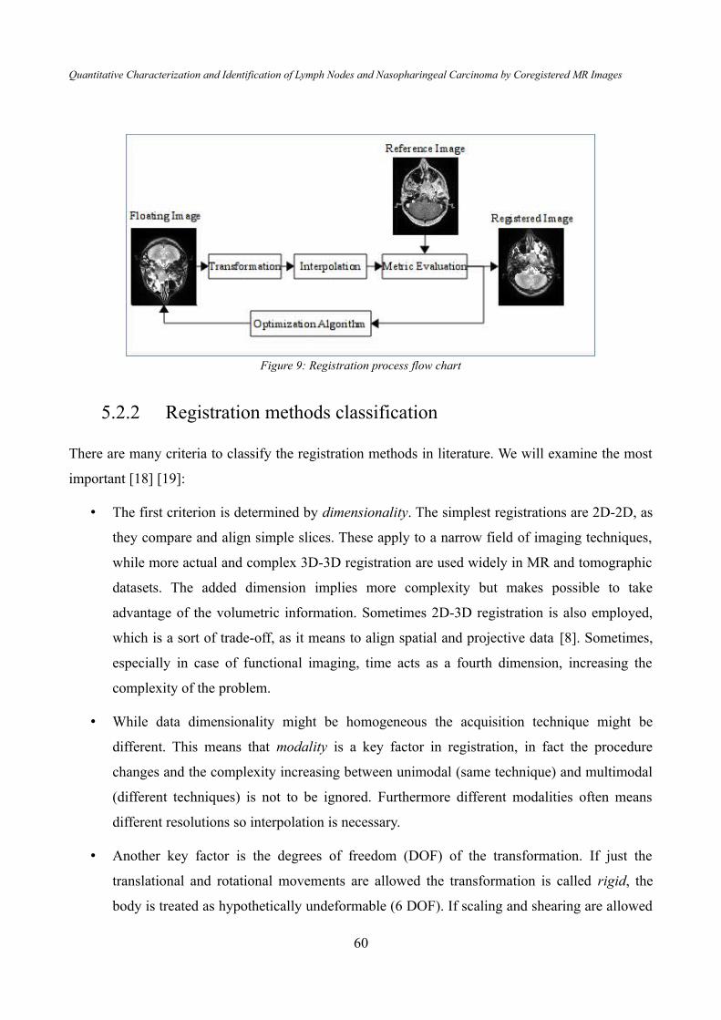
Quantitative Characterization and Identification of Lymph Nodes and Nasopharingeal Carcinoma by Coregistered MR Images
5.2.2 Registration methods classification
There are many criteria to classify the registration methods in literature. We will examine the most
important [18] [19]:
• The first criterion is determined by dimensionality. The simplest registrations are 2D-2D, as
they compare and align simple slices. These apply to a narrow field of imaging techniques,
while more actual and complex 3D-3D registration are used widely in MR and tomographic
datasets. The added dimension implies more complexity but makes possible to take
advantage of the volumetric information. Sometimes 2D-3D registration is also employed,
which is a sort of trade-off, as it means to align spatial and projective data [8]. Sometimes,
especially in case of functional imaging, time acts as a fourth dimension, increasing the
complexity of the problem.
• While data dimensionality might be homogeneous the acquisition technique might be
different. This means that modality is a key factor in registration, in fact the procedure
changes and the complexity increasing between unimodal (same technique) and multimodal
(different techniques) is not to be ignored. Furthermore different modalities often means
different resolutions so interpolation is necessary.
• Another key factor is the degrees of freedom (DOF) of the transformation. If just the
translational and rotational movements are allowed the transformation is called rigid, the
body is treated as hypothetically undeformable (6 DOF). If scaling and shearing are allowed
60
Figure 9: Registration process flow chart

Chapter 5. - Biomedical Images Registration
the transformation is called affine and the DOF double (12 DOF). The most general
transformation is called elastic or non-rigid, as it allows any deformation, giving to any
point of a grid 6 DOF.
Other classifications consider the data type (extrinsic or intrinsic methods), if the procedure relies
on the use of specific points (landmarks), segmented structures (image features), or the image grey
values (voxel based), or if there is an interaction (interactive, semi-automatic or automatic).
5.2.3 Transformation
When registering medical images one should always consider the DOF necessary to align the
intensity values available. The most important feature to think about is of course the mobility of the
district or the organ represented in the image itself. This is the biggest challenge in medical image
registration as the most tissues and organs of human body can accept huge deformation, bending,
can expand (due to physiological or pathological processes ) or reduce with many DOF.
Rigid and affine transformations can be described by a single matrix T considering the position p,
given the translational elements t x , t y and t z , is given by:
pnew=T rigid⋅pold=[r11 r12 r13 t x
r21 r22 r23 t y
r31 r32 r33 t z
0 0 0 1]⋅pold
where r ij are the elements of the rotational matrix:
R=R x⋅R y ⋅Rz =[1 0 00 cos −sin0 sin cos ]⋅[
cos 0 sin 0 1 0
−sin 0 cos ]⋅[cos −sin 0sin cos 0
0 0 1]In the affine case the scaling ( sij ) and the shearing ( h ij ) components have to be introduced in the
transformation matrix T :
pnew=T affine⋅pold=[r 11 r 12 r 13 t x
r 21 r 22 r 23 t y
r 31 r 32 r 33 t z
0 0 0 1]⋅[
s11 0 0 00 s22 0 00 0 s33 00 0 0 1
]⋅[1 h12 h13 00 1 h23 00 0 1 00 0 0 1
]⋅pold
61

Quantitative Characterization and Identification of Lymph Nodes and Nasopharingeal Carcinoma by Coregistered MR Images
For what concerns the non-rigid transform, as it is the most complex and general formulation, the
number of DOF is theoretically infinite and thus the representation cannot be a single T matrix.
5.2.4 Optimization algorithms
The parameters of a transformation process can be derived directly by solving a linear equation
system or calculated by an optimization function defined in the parameters space, which optimizes a
similarity-based cost function. Optimization algorithms are classified in two principal classes, the
first one does not require the calculation of the gradient function, while the second bases on the first
derivative computation [8]. The most important drawback of optimization method is the difficulty
of discriminate local and global minima. The algorithm is expected to converge on a local
minimum, but the solution is not unique as it depends on the starting point. To solve this issue can
be used different heuristics, for example it is possible to run the algorithm several times from
different starting points and choose the lowest minimum or to perturb the local minimum to see if a
global solution can be found [20]. In the following paragraphs we will examine only the most used
algorithms.
Downhill simplex
The downhill simplex method, developed by Nelder and Mead [8], requires only function
evaluation and not its first derivative. This strategy bases on the definition of a simplex, a
geometrical figure (in N dimensions) shaped by N+1 points interconnecting by line segments,
polygonal faces etc. Hence a 2D simplex is a triangle, in 3D a non necessarily regular tetrahedron.
This method is initialized with N+1 points defining a non-degenerate simplex. Setting one of them
as the starting point P0 , the other vertices are given by:
P i=P0e i ; i=0,... , N−1
where e i are N unit vectors and is the problem parameter. Different i can be defined for each
direction. The defined simplex is deformed iteratively by reflection, expansion and contraction steps
in order to define the minimum of the function f. The algorithm is repeated until the fractional
difference between the lowest and the highest function value evaluated at the vertices is smaller
than a fixed threshold.
62

Chapter 5. - Biomedical Images Registration
Conjugate-gradient descend
The conjugate-gradient method requires not only the calculation of the function f P but also the
gradient ∇ f P ; where P is an N-dimensional point.
The steepest descend method [20] start at point P0 and it moves from point P i to the point P i1
by minimizing along the line from P i in the direction of the local downhill gradient. The problem
of this method is that the gradient does not point to the optimum directly, but it performs several
small steps toward the minimum, even if the valley is a perfect quadratic form [8].
The conjugate gradient method overcomes the problem, building a new direction that is conjugate
to the previous one with respect to the function to minimize [21]. Following this method during
each iteration I a line minimization is performed in the direction h i , from the point P i to the point
P i1 . After each iteration a new direction h i1 is constructed by [20]:
h i1=g i 1i h i ; i=1,2 , ...
where
g i=−∇ f P i ; g i1=g i−A⋅h i ; i=1,2 , ...
Finally i and i are given by [20]:
i=g i⋅hi
hi⋅A⋅h i; i=
g i1⋅g i1
g i⋅g i
Quasi-Newton method
The quasi-Newton (or variable metric) method builds up iteratively a good approximation to the
inverse Hessian matrix A−1 of the N-dimensional function to optimize, in order to construct a
sequence of matrix H i with property [20]:
limi∞
H i=A−1
this procedure is necessary when an arbitrary function f x can be locally approximated as a
quadratic form by Taylor series [20]:
f x ≈c−b⋅x1/2 x⋅A⋅x
where both A and b are known.
63
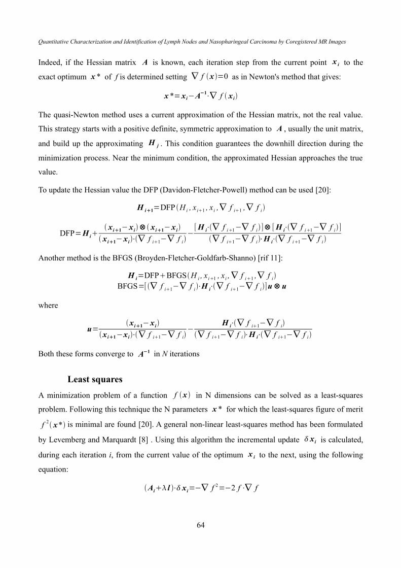
Quantitative Characterization and Identification of Lymph Nodes and Nasopharingeal Carcinoma by Coregistered MR Images
Indeed, if the Hessian matrix A is known, each iteration step from the current point x i to the
exact optimum x * of f is determined setting ∇ f x =0 as in Newton's method that gives:
x *=x i−A−1⋅∇ f x i
The quasi-Newton method uses a current approximation of the Hessian matrix, not the real value.
This strategy starts with a positive definite, symmetric approximation to A , usually the unit matrix,
and build up the approximating H j . This condition guarantees the downhill direction during the
minimization process. Near the minimum condition, the approximated Hessian approaches the true
value.
To update the Hessian value the DFP (Davidon-Fletcher-Powell) method can be used [20]:
H i1=DFP H i , x i1 , x i ,∇ f i1 ,∇ f i
DFP=H i x i1−x i⊗ x i1−x i
x i1−x i⋅∇ f i1−∇ f i−[H i⋅∇ f i1−∇ f i]⊗ [H i⋅∇ f i1−∇ f i]
∇ f i1−∇ f i⋅H i⋅∇ f i1−∇ f i
Another method is the BFGS (Broyden-Fletcher-Goldfarb-Shanno) [rif 11]:
H i=DFPBFGSH i , x i1 , x i ,∇ f i1 ,∇ f i
BFGS=[∇ f i1−∇ f i⋅H i⋅∇ f i1−∇ f i]u⊗ u
where
u=x i1−x i
x i1−x i⋅∇ f i1−∇ f i−
H i⋅∇ f i1−∇ f i
∇ f i1−∇ f i⋅H i⋅∇ f i1−∇ f i
Both these forms converge to A−1 in N iterations
Least squares
A minimization problem of a function f x in N dimensions can be solved as a least-squares
problem. Following this technique the N parameters x * for which the least-squares figure of merit
f 2 x* is minimal are found [20]. A general non-linear least-squares method has been formulated
by Levemberg and Marquardt [8] . Using this algorithm the incremental update x i is calculated,
during each iteration i, from the current value of the optimum x i to the next, using the following
equation:
Ai l ⋅ x i=−∇ f 2=−2 f⋅∇ f
64

Chapter 5. - Biomedical Images Registration
This technique can vary smoothly between the steepest descend and the inverse Hessian methods.
The behaviour is ruled tuning the constant : for values close to zero we have a inverse Hessian
method, while for large values it reduces to steepest descend.
Setting x to an initial position and approximating each element of the Hessian matrix by
Akl=2∇ f k⋅∇ f l , the following steps are resolved iteratively [8]:
1. Compute f 2 x i ;
2. Set a modest value for (e.g. =0.001 );
3. Solve the last equation for x i and evaluate f 2 x i x i ;
4. If f 2 x i x i≥ f 2
x i increase by a substantial factor (e.g. 10) and go back to step 3
5. Otherwise decrease by a substantial factor (e.g. 10), set x i1=x i x i and go back to
step 3
6. If f 2 decreases by a negligible amount the convergence is reached.
5.2.5 Similarity metric
As previously described, the registration process allows the spatial alignment of a reference and a
floating images. It is based on the minimization of a similarity function which gives informations
about the goodness of the matching. The similarity metric has to be robust, in order to converge to a
global maximum at correct matching, and has to be performed in a reasonable time.
Similarity functions can be classified according to the nature of registration: they can be feature
based or voxel based. In the following paragraphs we will examine the voxel based, as the feature
based are not as general and have not been employed in this thesis study.
Intensity difference
The simplest metric involves the definition of difference or absolute difference between two images
(mean square difference) [22] :
MQ A , B= ∑i , j belong S
ai−b j2
65

Quantitative Characterization and Identification of Lymph Nodes and Nasopharingeal Carcinoma by Coregistered MR Images
where i and j denote the corresponding voxels of the two images and S is the domain where both
images are defined.
Correlation
A widespread used metric is the normalized cross-correlation (NCC):
NCC=∑p∈S
A p−AB p−B
∑p∈S
A p−A2∑p∈S
B p−B2
where p denotes the position while A and B are the mean values of the A and B images
respectively. Hence a small difference in intensity is enough to give a large effect in the function
metric value. The main drawback of NCC is the high computational complexity. A speed
improvement can be obtained using a Fourier-domain based approach in NCC calculation: it is
possible, in fact, to compute the inverse of the cross power spectrum of the two images [23][24].
Entropy and mutual information
The mutual information (MI) is the voxel similarity function most used in biomedical image
registration. It comes from the information theory, and measures the dependence between two
variables or the amount of information that a variable contains about an other. Nowadays is the
more employed metric in the medical registration [25][26][27]. Indeed, this method does not require
any assumption and any constraints about the nature of the relation between the images. For this
reason the MI is a very general, powerful and robust metric for unimodal and multimodal spatial
alignment.
The mutual information is based on the Shannon entropy, that is a measure of information and it is
defined as [27]:
H=∑i
pi log1p i
=−∑i
pi log pi
where p i is the probability that an event takes place, and log 1/ pi is the amount of information
gained from a single event. For an image X, the probability p i is the occurrence distribution of
grey values calculated as the ratio between the number of times that each grey value occurs in the
image and the total number of voxels.
66

Chapter 5. - Biomedical Images Registration
The entropy definition becomes [22]:
H X =−∑xi∈ x
P X=x i⋅log [P X= x i]
The Shannon entropy is also a measure of dispersion because a distribution with a single peak will
give low entropy, while a dispersed distribution will yield a higher entropy value. Starting from this
definition the entropy can be used as measure of registration between images [28][29] exploiting the
histogram definition [30]. the joint histogram is a 2D matrix, showing the occurrence of each couple
of grey value in the image couple.
A joint histogram of two images can be used to estimate the joint probability distribution and then
the joint entropy of them [22] :
H X ,Y =−∑x i∈X
∑y j∈Y
log [P X= x i , Y= y j]⋅P X=x i , Y= y j
Most important than entropy in medical images registration, is the mutual information introduced
simultaneously by Viola and Collignon [26][31][32] and related to the image entropy. It is defined
as:
MI X ,Y =H X H Y – H X ,Y
All entropies must be evaluated in images overlapping parts, then the measures are sensitive to the
size of overlap. In order to reduce this sensitivity is advisable to employ the normalised MI:
NMI X ,Y =H X H Y
2 H X ,Y
In general MI is a non negative number and it is maximal when images are geometrically aligned.
The greatest advantage is the absence of any constraint on the acquisition modality, which makes
possible to align spatially images from different techniques, typical of multimodal registration.
5.2.6 A multi-level multimodal non rigid registration algorithm
developed by Reuckert, Sonoda et Al.[16]
Reuckert et al. published in 1999 a paper in which they proposed a new approach for the non rigid
registration of contrast enhanced breast MRI. The developed method was general and robust enough
that another paper in 2001 proved the reliability of the algorithm by applying it to other medical
67

Quantitative Characterization and Identification of Lymph Nodes and Nasopharingeal Carcinoma by Coregistered MR Images
registration issues [33]. This new registration method is based on two transformation: one describes
the overall motion with an affine transformation, the second provides a description of local
deformation based on a free form deformation (FFD) by employing B-splines [16]. Denoting with
x, y, z the 3D coordinates system axes, while T is the transformation that links the images A and B:
T : x A , y A , z Ax B , y B , z B
therefore we can state:
T x , y , z =T global x , y , z T local x , y , z
Global motion model
The global motion model describes the overall motion of the interest volume. The simplest choice is
a rigid transform which defines 6 DOF, describing just rotations and translations. A more general
transform is advisable, which describes shearing and scaling, thus an affine transform can be
defined:
T global x , y , z =11 12 13
21 22 23
31 32 33
xy
z 14
24
34
where the parameters define the 12 DOF of the transform. In this way the motion model can be
extended to higer order global transformations such as trilinear or quadratic [16].
Local motion model
The affine transformation captures only the global motion, thus a more detailed model is necessary
to describe the local deformation. It is difficult to describe these motions via parametrized
transformations, thus a FFD model, based on B-splines is a powerful tool for modeling 3D
deformable objects. The basic idea behind FFD is to deform an object by manipulating an
underlying mesh of control points. The resulting deformation controls the shape and produces a
smooth and C2 continuous transformation.
To define the spline based FFD, we denote the domain of the image volume as:
={x , y , z ∣0≤x≤X ,0≤ y≤Y ,0≤ z≤Z }
while denotes a nx×ny×nz mesh of control points i , j , k with uniform spacing .
68

Chapter 5. - Biomedical Images Registration
Then, the FFD can be written as the 3D tensor product of the 1D cubic B-splines:
T local x , y , z =∑l=0
3
∑m=0
3
∑n=0
3
B lu Bm v Bnwil , jm ,kn ; i=[x /nx]−1 ; u= x /nx – [ x /nx ];j=[ y / ny ]−1 ; v= y /n y – [ y /ny ];
k=[ z / nz ]−1 ; w=z /n z – [ z /n z] ;
where Bl represent the l-th basis function of the B-Spline:
B0 u=1−u3/6
B1u=3u3 –6u24/6
B2u=−3u33u2
3u1/6
B3u=u3/6
In contrast with other splines, B-splines are locally controlled, which makes them computationally
efficient even for a large number of control points. In particular, the basis functions of cubic B-
splines have a limited support, i.e., changing control point i , j , k affects the transformation only in
the local neighbourhood of that control point.
The control points act as parameters of the B-spline FFD and the degree of non rigid
deformation which can be modeled depends essentially on the resolution on the mesh of the control
points . A large spacing of control points allows modeling of global non rigid deformations,
while a small spacing allows modeling of highly local non rigid deformations. At the same time, the
resolution of the control point mesh defines the number of DOF and, consequently, the
computational complexity. The tradeoff between model flexibility and computational complexity is
mainly an empirical choice which is determined by the accuracy required versus the increasing in
computation time. In order to achieve the best compromise a hierarchical multiresolution approach
has been developed, in which the resolution of the control mesh is increased, along with the image
resolution in a coarse to fine fashion.
Let 1 ,... , L denote a hierarchy of control point meshes at different resolution, in which as the
index increases (from 1 to L) the point spacing decreases. To avoid the overhead of calculating
several B-spline FFDs separately, we represent the local transformation by a single B-spline FFD
whose control point mesh is progressively redefined. In this case, the control point mesh at level l is
refined by inserting new control points to create the level l1 mesh. A common procedure is to
halve the control point spacing at each level. In this case, the position of control point 2i,2 j ,2kl1
coincides with that of control point i , j , kl and the values of the new control points l1 can be
calculated directly from those of l , using a B-spline subdivision algorithm.
69

Quantitative Characterization and Identification of Lymph Nodes and Nasopharingeal Carcinoma by Coregistered MR Images
To constrain the spline-based FFD transformation to be smooth, one can introduce a penalty term
which regularizes the transformation. In 3D the penalty term takes the following form:
C smooth=1V ∫0
X
∫0
Y
∫0
Z
[∂2 T
∂ x2 2
∂2T
∂ y2 2
∂2T
∂ z 2 2
2 ∂2 T∂ xy
2
2 ∂2T∂ yz
2
2 ∂2T∂ xz
2
]dx dy dz
where V denotes the volume of the image domain. This quantity is the 3D counterpart of the 2D
bending energy of a thin plate and defines a cost function which is associated with the smoothness
of the transformation.
Optimization
To find the optimal transformation, we minimize a cost function associated with the global
transformation parameters , as well as the local transformation parameters . the cost function
comprises two competing goals. The first term represents the cost associated with the image
similarity C similarity while the second term corresponds to the cost associated with the smoothness of
the transformation C smooth :
C ,=−C similarity A ,T BC smoothT
Here is the weighting parameter which defines the tradeoff between the alignment and the
smoothness of transformation. It is also observable that the intrinsic smoothness properties of B-
splines mean that the choice of is not critical for low resolutions of the control point mesh. The
regularization term is more important for high resolutions.
70

Chapter 5. - The Nasopharyngeal Carcinoma
5.3 The Nasopharyngeal Carcinoma
Nasopharyngeal carcinoma (NPC) is a squamous cell carcinoma that usually develops around the
ostium of the Eustachian tube in the lateral wall of the nasopharynx. Though rare among whites,
NPC is particularly common in the southern Chinese population of Guangdong, Inuits of Alaska,
and native Greenlanders [1]. Chinese emigrants continue to have a high incidence of the disease,
but the rate of NPC among ethnic Chinese born in North America is considerably lower than those
born in China. This epidemiologic evidence implies that both environmental factors and genetic
susceptibility play roles in the development of NPC [1]. The environmental factors may include
exposure to nitrosamines in salted and pickled foods. Certain human leukocyte antigen subtypes
have been associated with NPC, as they have various genetic polymorphisms [1].
5.3.1 Classification
The World Health Organization classifies NPC based on histology [1]
• Type 1, keratinizing squamous carcinoma, is characterized by well-differentiated cells that
produce keratin.
• Type 2, nonkeratinizing squamous carcinoma, varies in cell differentiation but does not
produce keratin.
• Type 3 is also nonkeratinizing, but is less differentiated, with highly variable cell types
(clear cell, spindle cell, anaplastic).
Types 2 and 3 NPC are Epstein–Barr virus (EBV) associated and have better prognoses than type 1;
EBV infection is generally absent in type 1, especially in nonendemic areas. However, more recent
data state that almost all NPC tumors, regardless of histologic subtype, have comorbid EBV
infections, which is strong evidence for EBV as the etiology of NPC. This close association with
EBV is what makes NPC unique from other head and neck cancers.
71

Quantitative Characterization and Identification of Lymph Nodes and Nasopharingeal Carcinoma by Coregistered MR Images
5.3.2 Treatment
Standard treatment for NPC is radiotherapy, but concurrent adjuvant chemotherapy improves
survival rates. As with other cancers, the prognosis of NPC depends upon tumor size, lymph node
involvement, and distant metastasis (TMN staging). But NPC, in contrast to other head and neck
malignancies, is highly sensitive to radiation and chemotherapy [1].
High survival rates are reported for stage 1 and 2 diseases, but the prognosis for metastatic disease
remains poor even with combined radiation and chemotherapy treatment, with disease relapse rates
as high as 82% [1]. Unfortunately, the majority of NPC is diagnosed at an advanced stage because
of non specific presenting symptoms (cervical nodal enlargement, headache, nasal and aural
dysfunction), delay in seeking treatment after the onset of symptoms, and the difficulty of a
thorough nasopharyngeal exam. In light of this, more targeted treatments of NPC need to be
developed.
5.3.3 Epstein–Barr Virus
EBV is a g-herpes virus present in over 90% of adults worldwide [1]. Though the infection is life-
long, it usually remains harmless unless the balance between host and virus is altered. Diseases
associated with EBV include those of lymphocytic origin (infectious mononucleosis, Hodgkin’s
disease, and Burkitt’s lymphoma) and epithelial origin (NPC, oral hairy leukoplakia, and
undifferentiated gastric carcinoma) [1]. At least 95% of NPC tumors are EBV associated.
Additionally, the severity of EBV infection varies with carcinoma type, with undifferentiated
carcinomas having the highest EBV titers. EBV has tumorigenic potential due to a unique set of
latent genes: latent membrane proteins (LMP1, LMP2A, and LMP2B) and EBV-deter mined
nuclear antigens (EBNA1 and EBNA2) are the proteins predominantly expressed in NPC [1].
LMP1 is the principal oncogene of NPC it is required for cell immortalization and is present in 80%
to 90% of NPC tumors. The LMP1 molecule includes 6 transmembrane domains and a carboxy-
terminus containing 2 signaling domains called C-terminal activating regions 1 and 2 (CTAR 1 and
2). The transmembrane domains allow LMP1 to associate with the host membrane, whereas the
CTAR regions directly activate a number of signaling pathways including nuclear factor j-B (NF-
jB), mitogen-activated protein (MAP) kinases, and phosphoinositol-3-kinase (PI3K). Although the
basic role of LMP1 is to prevent apoptosis, it has other important functions in cancer development.
72

Chapter 5. - The Nasopharyngeal Carcinoma
LMP1-positive cells have greater mobility, leading to higher metastatic potential and faster disease
progression. LMP1 is also involved in suppressing immunogenic responses against NPC; for
example, LMP1 has intrinsic T-cell inhibitory properties and mediates downregulation of CD99,44
an important component of the anti-NPC immune response. The importance of LMP1 in
tumorigenesis is illustrated by numerous studies that show the inhibition of LMP1 results in
increased tumor cell sensitivity to chemotherapy [1].
Less is known about LMP2 and EBNA than LMP1, but with recent research their role in EBV-
induced tumorigenesis is becoming more understood. Previously it was thought that LMP2
probably only mediated tumor cell survival; however, newer data show that LMP2, particularly
LMP2A, has more diverse functions. LMP2A downregulates the NF-jB transcription factor and can
decrease LMP1 expression. Additionally, LMP2A expression causes NPC cells to become
migratory and invasive. EBNA1 is an unusual protein that binds the EBV genome to host
chromosomes, and thus mediates equal partitioning of viral DNA into daughter cells during cell
division and may play a role in immune evasion [1]. EBNA2 may be involved in the transactivation
of LMP1.
5.3.4 Overview
The mechanism of NPC tumorigenesis is complex, involving the aberrations of a large variety of
pathways and the alteration in expression of numerous proteins. Normal regulation of apoptosis,
cell proliferation, and cell adhesion are dysregulated. The understanding of these mechanisms has
greatly increased in the past decade, generating enough data to begin the development of prognostic
factors and targeted treatments for NPC. Refining prognostic factors into clinically applicable
assays may aid in the detection of NPC in asymptomatic patients, in addition to staging and
monitoring disease. The search for molecularly based treatments for NPC has only just begun, and
so much is yet to be discovered. Improved understanding of the unique molecular mechanisms
behind NPC will hopefully lead to the development of targeted treatments against NPC that slow
disease progression and improve survival[1].
73

74

6.Materials and Methods
This research study has been developed as Biomedical Engineering degree thesis at the Politecnico
di Milano, in close collaboration with the “Fondazione IRCCS Istituto Nazionale dei Tumori”
(INT). The work was developed in the “Laboratory of Advanced Radiologic Analysis” (LARA),
born in 2003 as a collaboration between the “Dipartimento di Biongegneria” del Politecnico di
Milano and the Department of “Diagnostica per Immagini e Radioterapia” of the INT.
6.1 Experimental Protocol
The study has been carried out on 15 patients affected by rinopharingeal carcinoma, 3 females and
12 males, aged between 14 and 60 at the moment of the MR examination. 14 of them underwent
radiotherapy and/or chemotherapy and had being examined after each step planned by the therapy.
The average patient examination sessions are three, with a minimum of only one to a maximum of
10 session. Usually the sessions are separated by a variable period from 3 to 12 months depending
on several clinical factors.
Among the available clinical cases the selected patients satisfied the following criteria:
• The presence of MR examination at diagnosis, aiming to evaluate the status or to confirm
the presence of a suspect carcinoma
• The availability of the whole multimodal examination (see below)
• Absence of artefacts on the images (i.e. due to dental prosthesis or patient movement)
75

Quantitative Characterization and Identification of Lymph Nodes and Nasopharingeal Carcinoma by Coregistered MR Images
In any case the purpose of this study was not to find clinical evidences about the pathophysiological
state of the lesion, but to identify the pathological tissues or features clearly visible in diagnosis.
6.1.1 Exams and biomedical images
The standard protocol in these clinical cases plans the acquisition of these sequences:
• T1 VIBE, for the whole head and neck district. This is a T1 weighted with Gadolinium
contrast agent 3D acquisition, with isotropic 0.65mm resolution; RT=5.23ms, ET=2.05ms.
• T1 TSE for maxillo-facial and for neck volumes separately. This sequence is a T1 weighted
Turbo Spin Echo 2D multi-slice axial acquisition, with 4mm slice spacing, 0.65mm planar
resolution; RT=572ms; ET=12ms.
• T2 TSE for maxillo-facial and for neck volumes separately. This sequence is a T2 weighted
Turbo Spin Echo 2D multi-slice axial acquisition, with 4mm. slice spacing, 0.5mm planar
resolution; RT=3180ms; ET=109ms.
• DWI serie, which includes the DW images with b-values from 0 to 1000 (0, 300, 500, 700,
1000), taken separately for head and for neck volumes. This sequence is a DW EPI 2D
multi-slice axial acquisition, with 5mm slice spacing, 2mm planar resolution; RT=5200ms;
ET=79ms.
Except the 3D anatomical T1, the other sequences were acquired by axial slices and in two separate
volumes. The first volume depicts the head district, while the second the neck: this means that the
acquisition of the two volumes is distinct and separated by a short but non negligible amount of
time. Further the acquisition protocol of the neck district implies a different normal orientation
compared to the head, while volumes are overlapped in the junction region. Globally a complete
exam session is composed by 15 volumes: an anatomical isotropic sequence, a two axial T1
volumes, a two axial T2 and 5 couples of DW images.
The images were acquired with a Siemens 1,5T Magnetic Resonance Machine. The data was stored
in the Institute PACS (Picture Archiving and Communication System) also developed by Siemens
with the commercial name of Syngo. Before any further analysis the DICOM images, which was
retrieved from the archiving system, were treated to delete all sensible fields. This to provide the
right privacy, according to the Italian law [34].
76
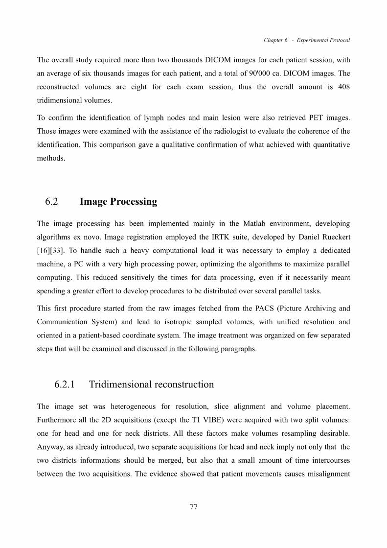
Chapter 6. - Experimental Protocol
The overall study required more than two thousands DICOM images for each patient session, with
an average of six thousands images for each patient, and a total of 90'000 ca. DICOM images. The
reconstructed volumes are eight for each exam session, thus the overall amount is 408
tridimensional volumes.
To confirm the identification of lymph nodes and main lesion were also retrieved PET images.
Those images were examined with the assistance of the radiologist to evaluate the coherence of the
identification. This comparison gave a qualitative confirmation of what achieved with quantitative
methods.
6.2 Image Processing
The image processing has been implemented mainly in the Matlab environment, developing
algorithms ex novo. Image registration employed the IRTK suite, developed by Daniel Rueckert
[16][33]. To handle such a heavy computational load it was necessary to employ a dedicated
machine, a PC with a very high processing power, optimizing the algorithms to maximize parallel
computing. This reduced sensitively the times for data processing, even if it necessarily meant
spending a greater effort to develop procedures to be distributed over several parallel tasks.
This first procedure started from the raw images fetched from the PACS (Picture Archiving and
Communication System) and lead to isotropic sampled volumes, with unified resolution and
oriented in a patient-based coordinate system. The image treatment was organized on few separated
steps that will be examined and discussed in the following paragraphs.
6.2.1 Tridimensional reconstruction
The image set was heterogeneous for resolution, slice alignment and volume placement.
Furthermore all the 2D acquisitions (except the T1 VIBE) were acquired with two split volumes:
one for head and one for neck districts. All these factors make volumes resampling desirable.
Anyway, as already introduced, two separate acquisitions for head and neck imply not only that the
two districts informations should be merged, but also that a small amount of time intercourses
between the two acquisitions. The evidence showed that patient movements causes misalignment
77

Quantitative Characterization and Identification of Lymph Nodes and Nasopharingeal Carcinoma by Coregistered MR Images
between head and neck in this divided acquisition. Thus merging informations by resampling head
and neck slices together causes blurring and artefacts.
The procedure chosen (Figure 10) was to first resample the head and neck volume separately,
perform an alignment respect to the anatomical T1 VIBE volume and then fuse the two districts in
an unique volume. Finally adding a non rigid transform made possible to correct residual patient
movement (i.e. neck flexion or extension).
78
Figure 10: Image processing from 2D DICOM to coregistered 3D volumes.

Chapter 6. - Image Processing
The first step of images reconstruction consisted in rototranslating every single planar image,
applying a transformation that project the intensity values from the image-coordinates space to the
patient-coordinates one. This crucial information was calculated directly from IOP (Image
Orientation Patient) and IPP (Image Position Patient) values included in the DICOM header. After
this transformation the MR slices can be placed in the patient-coordinates space which is imposed
by the operator during the acquisition procedure. What results from this process is a large number of
points, identified by tridimensional patient coordinates and described by an intensity value, not
ordered in an axis-oriented grid, and with a custom resolution (Figure 11). At this point it was
possible to impose an isotropic sampling grid, with an higher resolution (0.5mm). This resolution
was chosen to not loose the information at higher resolution.
The data resampling revealed to be effort taking and time consuming: more than 108 samples to be
processed to obtain 109 samples by a linear interpolation puts even a high-rank PC under a too
heavy load. Dividing the data to smaller volumes (about 106 samples), with 1/8 of overlapping along
79
Figure 11: Example of tridimensional DICOM alignment for T1 examination. It is visible how the stacked images reproduce the silhouette of the patient. The slices of the head and the neck sequences have different normals, they are compenetrated in the conjunction area, but not aligned to the x-y plane in patient coordinates. All quotes are in mm.

Quantitative Characterization and Identification of Lymph Nodes and Nasopharingeal Carcinoma by Coregistered MR Images
each dimension, makes the computation (especially the search of tetrahedron vertexes, see below)
very lighter and makes possible to run several parallel tasks. Overlapping indeed avoids
discontinuity in the final output, at the cost of some overhead in computing. Anyway this avoided
the CPU overload and reduced data caching on the hard drive.
The interpolation was implemented employing Matlab function called TriScatteredInterp. This
routine creates an interpolant surface using a Delaunay triangulation [35]: each point of the data
becomes the vertex of one or more tetrahedron, and the final structure is known to be unique and to
show the Empty Sphere Property: “no node lies in the interior of the circumscribed sphere of a
simplex” (in this case a tetrahedron) “of the triangulation ” [36]. This leads to a very fast calculation
of an interpolant, which requires for our purpose a linear interpolation. Even if a smoother and C1
continuous interpolation was desirable the rising complexity of the problem would have increased
enormously the computation timings.
At the end of this procedure our volume is reconstructed on the isotropic axis-oriented grid, with
resolution of 0.5mm. This was repeated for each subvolume, avoiding overlapping, thus the final
volume was composed by placing those data side by side. At this point all the volumes were
converted from 3D matrix to Nifti Image file format (NII) [37]. In this binary data file is included
an header containing information about resolution, position, orientation, image depth etc. as well as
values of each voxel, ordered by their tridimensional position. The Nifti Image format have
standard definition, representing 3D or 4D volumes, in grayscale or RGB space, thus allowing 7D
data as maximum in storing. The precision of the values is variable, in this study we used 16-bit
integers to describe voxels. This was made to preserve the original grayscale resolution without
increasing the volume storage size. Concordantly to the volume reconstruction in 3D space the
spatial information were recoded in the file header as volume centre coordinates.
The final result of the Tridimensional Reconstruction step is that all the exams of the session are
translated in the patient-based coordinates system, linearly interpolated to a resolution of 0.5mm in
isotropic voxels. Each final volume, saved as Matlab matrix, is obtained in a time between 10
minutes and 50 minutes, depending on the native resolution.
80

Chapter 6. - Image Processing
6.2.2 Images registration technique
The registration steps have been implemented by IRTK, supervised and scheduled by Matlab. In
these procedures the template image was the one acquired with the T1 VIBE sequence. This
because it has the best native resolution (isotropic 0.6mm) and it is commonly used by physicians to
evaluate the anatomic detail. Even if the contrast modes of T2 and DWI are not correlated to the T1
anatomical image, their informational contents are coherent with the anatomical image. Thus, using
an information-depending similarity index such as NMI, the T1 VIBE derived volume can be
employed to correctly register the volumes.
Exams taken in each sessions, after resampling, were similar. Anyway DWI images have the
advantage of being acquired simultaneously per b-value: alignment can be evaluated on one b-value
and then applied to all the other. Since at this level of processing no actual difference is brought by
the contrast modality of the images (T1, T2 or DWI), it is reasonable to consider them the same
way. The registration designed was multilayer multimodal multiresolution rigid and non rigid, based
on the algorithm described in [16] and detailed in the previous sections . The routine has been
organized in four consequent steps: a rigid undersampled transform with a smoothed template, a
second rigid transform with higher resolution on a non-smoothed template, the head and neck
volume merging and a final non-rigid transform on a smoothed template. In the three registration
the similarity metrics used is NMI, computed on the 32-bin histogram and cross-histogram, while
the optimization function employed a conjugated gradient descend. Hence we obtained a good
similarity estimate even when different MR modalities were compared (T1 versus T2 or T1 versus
DW), and reduced the NMI computation time, which rises fast as when the number of histogram
bins increases.
Rigid transforms on smoothed and non-smoothed template
This two rigid transforms had the aim to coarse align the volumes to the anatomical image,
correcting patient movements both between modality changes and between head and neck
acquisition. The first multiresolution transform was estimated on undersampled images. The
template was obtained from the T1 VIBE exam, after the application of a gaussian kernel smoothing
with a σ=2.5mm . The resolution steps were 5mm and 2.5mm. The second rigid transform was
computed on the non smoothed template, with two resolution steps. The resolution levels were 1mm
81

Quantitative Characterization and Identification of Lymph Nodes and Nasopharingeal Carcinoma by Coregistered MR Images
and 0.5mm. This step had the aim to correct the residual patient rigid movement, without image
blurring.
Head and neck merging
Before the last registration step the head and neck volumes were merged. This, thanks to the
alignment already computed, was implemented by a simple mean of non null values. Zeros were
excluded to avoid image darkening near the junction, this avoided the most evident border effects.
Non-rigid transform on smoothed template
In the last of the three steps a non-rigid transform was estimated. Even if in the head district non
rigid movements are few, this does not hold for the neck (i.e. flexion and extension). The
transformation was estimated on a smoothed template (obtained by a gaussian filter with σ=3mm )
and undersampled to a resolution of 5mm and 3mm. The control points mesh for the B-splines
calculation was sparse, isotropically placed every 200mm. This configuration was to identify the
wide deformations, mainly identifiable by aligning muscles and spinal cord, and not to introduce
too sharp deformations. Further when registering DW versus T1 VIBE the floating image well
contrasted areas are few compared to the template: too flexible registrations could have led to a
excessive deformation.
Since the non rigid step was particularly time consuming, when evaluating the NMI only voxels
with intensity over a threshold were considered. This limited data loss was affordable in front of the
reduction of computational time, as no sensible registration worsening was shown. The threshold
value is an estimation of the maximum background noise in T1, T2 and DW images obtained by
82
Figure 12: Examples of images histograms compared to the threshold. Form left to right: DWI, T1 and T2. The red line depicts the threshold=50.

Chapter 6. - Image Processing
comparing the histograms of the resampled volumes (Figure 12). The threshold value of 50 showed
to be a good compromise.
The final step was obviously to apply the computed transform to the image. In particular this last
phase introduced another resampling, due to admit the displacement of rototranslated points. The
output is still a 3D Nifti Volume, where the resolution and the coordinates of the sampling mesh are
the same of the template, which means 0.5mm resolution and the boundaries of the T1 VIBE
volume.
DWI
Concerning DWI, the sequence variation that leads to b-value changing is made once per slice. This
means that the b-value changes with a period equal to TR and lower than slice to slice acquisition
interval, which is assumed to be quasi-instantaneous, or at least negligible looking at the patient
movement. Thus we can make the assumption that all the DWI volumes, whatever the b-value is,
are already aligned one respect the others. Hence we can register just the lowest b-value volume
available, where the visible structures, even if with still very low detail, are many more than the
higher b-values.
6.2.3 Optimization notes
As in the reconstruction process was split in parallel tasks by dividing the overall volume in
subvolumes to reduce resampling time, the registration routine was designed in parallel tasks too.
The main difference though is that a single volume should not be divided in subvolumes and has to
be registered as-is. Another constrain was the causality in the registration routine. Each of the three
steps needed the previous one to be completed, so they could not be performed in the same time.
So the parallelism was developed making several registrations in the same time, one task for each
modality volume.
For what concerns the head and neck volumes, they had both to be registered before being merged,
so it could be possible to take advantage of the parallelism in the rigid transforms estimation and
application. After merging though, the parallel tasks were halved, due to the merging itself, so just
half of the available computing power was employed actively.
83

84

7.Quantitative Characterization and Identification of Lymph
Nodes and Carcinoma Tissues
In this study, after the image fusions described in the previous chapter, we propose a method to
identify the tissues of clinical interest. This method is based on MRI routine protocol images only
and semi-automatic, requiring the radiologist intervention in the identification of two ROIs: one
located on lymph node, the other in carcinoma tissues. Then the informations obtained by these
ROIs lead to a recognition of similar tissues in the district of interest. The output is a probability
map, which attributes each voxel to a given tissue. The maps are aligned to the whole image set and
thus easily comprehensible by the clinicians.
7.1 Supervised Tissue Location and Characterization
This whole supervised identification task was performed on diagnosis exam sets only, but the
information obtained can also be used to segment successive MR examination.
The first step of this method was the identification of tissues of interest. As easily understandable,
the slight but non negligible difference in intersubject tissues (pathological and non pathological)
causes an hypothetical completely automatic, method to fail due to both false positives or false
negatives classifications. Therefore the identification of tissues of interest was taken with the
supervision of an experienced radiologist. A graphical interface was developed for this purpose.
85

Quantitative Characterization and Identification of Lymph Nodes and Nasopharingeal Carcinoma by Coregistered MR Images
7.1.1 Graphic user interface and tissue location
This graphic user interface (GUI), implemented in Matlab environment, with the aim to furnish a
simple and easy to use layout (Figure 13). Thus the window is unique (no popups or palettes), and
based on few tool buttons, nevertheless it allows the navigation in the volume by visualizing all the
three clinical planes (axial, sagittal and coronal) continuously, even when panning and zooming the
tridimensional volume.
The two tissues to be located have substantial differences. Lymph nodes are usually spheroids with
variable dimensions, the carcinoma at diagnosis appears as a defined extraneous mass in the
nasopharynx. Hence different strategies was used for carcinoma and lymph nodes location.
The main carcinoma lesion tissue was located by a parallelepiped (a cube by default) customizable
in 6 parameters: 3 sizes and 3 position coordinates. No rotation or shears of the parallelepiped was
allowed to avoid a complexity increment. In fact shears and rotation may introduce a problem of
86
Figure 13: The GUI employed to define the tridimensional ROIs. The coloured regions represent the boundary of the 3D parallelepiped defining the template.

Chapter 7. - Supervised Tissue Location and Characterization
boundaries (shape adaptation to a finite voxels grid) and resampling, and thus we excluded them.
The parallelepiped shape was defined with three bidimensional adjustment of rectangular selections,
each on a clinical plane, finally an overview check was performed with a simple video composed by
visualizing a projection while sweeping with the slicing plane the entire selection volume.
Lymph nodes tissue was located considering the internal region of few active lymph nodes. This
was implemented to characterize the inner parts of those structures as they are one of the most
interesting features in the evaluation of pathological course. In particular the ROI was a cube of
4.5mm (9 voxel) side, inscribed in a clearly visible active lymph node. This procedure was repeated
for few sites (from 2 to 5) depending on lymph nodes dimension and visibility, but ensuring enough
data to define the template of tissue features, according to the clinician judgement.
7.2 Quantitative Identification
In clinical practice an experienced radiologist uses four kind of images to investigate and eventually
identify the carcinoma and the lymph nodes: T1 and T2 weighted images, an anatomical T1 with
contrast medium and the diffusion images (natively or subsumed in the ADC map). In this study we
decided to rely on the same features that the experienced observation can identify in each contrast
modality and emulate the radiologist decision making with a quantitative method. Since each
contrast modality brings a particular information such as the kind of cellularity, the morphology and
the anatomy of the visible features, the main chemical composition (liquid, fat, muscle, bone, etc.)
their intensity values can give a synthetic description of the examined area. This is also true for the
rest of the examined body district, which is the basic principle beyond the quantitative identification
algorithm implemented.
7.2.1 Characterization of tissue templates
Once the tissue had been located they had to be characterized quantitatively. At this purpose we
relied on four different informations brought by the set of images examined:
• T1 weighted voxels intensity;
• T2 weighted voxels intensity;
87

Quantitative Characterization and Identification of Lymph Nodes and Nasopharingeal Carcinoma by Coregistered MR Images
• T1 VIBE (with contrast) anatomical tissue appearance;
• DWI images (collected with five b-values).
Actually in clinical practice DWI are used mainly to compute the ADC map, through an exponential
fitting of the curve described by each b-value image. In this study we decided to employ “raw”
diffusion data coming from the DWI volumes to avoid data approximation or interpretation.
The intensity values of the areas described during tissue location have been used to define a
probability function, which quantifies the membership of a voxel to the tissue. Looking at this task
from a statistical point of view, the frequency of voxel intensity can characterize the regions of
interest. Thus the intensity histogram taken from template tissue has been considered to define those
probability values.
7.2.2 From template histograms to membership functions
The statistic frequency represented in histograms can be interpreted both as composition of template
tissues and probability of a voxel to represent the same tissue of the template. A rigorous statistic
method would make use of Bayes theorem, however the space in which the problem resides is 8-
dimensional (one dimension for each image), which increases enormously the complexity. It is
enough to consider a multivariate histogram to describe joint distributions of probability: when we
would identify 32 bin for each dimension the overall bins we would describe the data with will be
328=1,09⋅1012 .
The implemented method was fuzzy-like, and responded to the obvious question: “What does the
interest tissue look like?”. To give a good answer we can imagine to have a “recipe” for our tissue
(identified in the template), and thus to know the quantity of each “ingredient”(voxel intensity in
each modality).
The recognition used eight unidimensional membership functions (one for each image), derived by
normalizing the amplitude of the ROI histogram between 0 and 1. Let's define the plain (non-
multivariate) histogram: h jROIk is the number of voxels in the j-th image whose intensity value is
k , where k varies continuously along whole the intensity range with the same bin resolution of the
original j-th image. To reduce problem related to bin size and voxel number the histograms were
smoothed with a 5-samples symmetric non-padded moving average.
88

Chapter 7. - Quantitative Identification
The membership function is defined as:
M j I j x , y , z =h j
ROI I j x , y , z
maxkh j
ROIk
where I jx , y , z is the intensity of voxel of coordinates x , y , z in the image j. This function
assumes the highest membership values where the intensity of the voxels is close to the maximum
of h jROIk . Correspondingly lower membership scores are given to intensity values corresponding
to less frequent voxels in ROI, while 0 is given to the rest of the values.
7.2.3 Identification map
The contribute of each membership function was combined with the same weight to generate the
final score. This choice gave an higher importance to the DWI contributions (5 of 8 images), and it
is justified by the patophysiological and diagnostical importance of the diffusion dynamic for tissue
characterization. This, in fact, can distinguish highly diffusive areas, which might be pathological,
from the rest of the tissues. Furthermore DWI carries information through the b-values dynamic,
thus including the whole DWI images set, as it was, meant to not reduce or modify the
informational content.
The raw identification map P v was the sum of each membership value, scaled between 0 and
1000:
P v =∑j=1
8
M j I jv ⋅1000
8
where v is the position of the voxel in the whole patient space. This was to give a simple value
range, easily understandable and comparable between different patients or sessions.
The final map was obtained imposing a threshold value to cut the surely non significant matches:
P v ={ P v P v th0 otherwise}
where th=250 .
As the tissues of interest were two, this procedure was performed twice, hence we obtained an
identification map based on the lesion template while the other was based on lymph nodes template.
89

90

8.Results
The first result of this study was the fusion of the MR examination images. Relying on this sets of
fused volumes it was possible to develop the algorithm (described in the previous chapter) to
compute tissue identification maps. In the following paragraphs we will introduce a statistic
examination of registration performance. Then we will examine the maps features, evaluating their
behaviour in relation of pathological structures. In the last section we will compare PET images and
maps identification performance for lymph nodes and carcinoma.
8.1 Image registration
At each step of registration we computed NMI and NCC values to keep a trace of the performance
of the procedure. The choice of these two similarity metric was made as they are widely used in
literature to evaluate image registration performance. These indexes were evaluated on the image
overlapping area described by a 250 voxel-sided cube located around the centre of the target image.
For what concerns NCC it was obtained directly with the equation given in the second chapter. NMI
was computed from 128 bins (versus the 32 employed in registration) histograms and cross-
histogram, to improve the detail of informational content of NMI.
91

Quantitative Characterization and Identification of Lymph Nodes and Nasopharingeal Carcinoma by Coregistered MR Images
Values were computed at every step of the multilevel registration procedure: before alignment (1),
after first rigid transform procedure (2), after the second rigid procedure (3) and at the end of the
process (4). The four values were obtained for each image modality. The results are shown in graph
(Figure 14). As it appears from the data shown, NMI describes a registration improvement, while
NCC has a more variable trend. The largest difference is the worsening of mean NCC in steps 3 and
4 for T1 and T2 volumes. This can be explained as NMI and NCC rely on different principles: while
NMI is informational based, NCC is intensity based. NCC, in fact, assumes negative values for
aligned but counter-phase image patterns. This condition is particularly significant in T1 and T2
registrations, while DWI seems not to suffer much this problem.
The improvement from raw data to first rigid alignment is noticeable (steps 1-2 in Figure 14), in
this step the wide translational and rotational differences are corrected efficiently. The second rigid
transform (step 3) gives a smaller improvement as it performs the residual alignment. The higher
resolution and the clear improvement of the previous step imply that only smaller alignment steps
have to be taken. Finally the non rigid alignment can correct the wide deformation due to patient
movements, hence it shows the last wide improvement in similarity measures (step 4).
92
Figure 14: Similarity metrics (mean values ± standard deviation) for raw data (1), after first rigid transform (2), second rigid transform(3), and non rigid transform (4). On the top row NCC, on the bottom one NMI, while from left to right T1, T2 and DWI statistics. These data trends show the improvement in alignment, considering that NCC performances are limited in case of multimodal image registration .
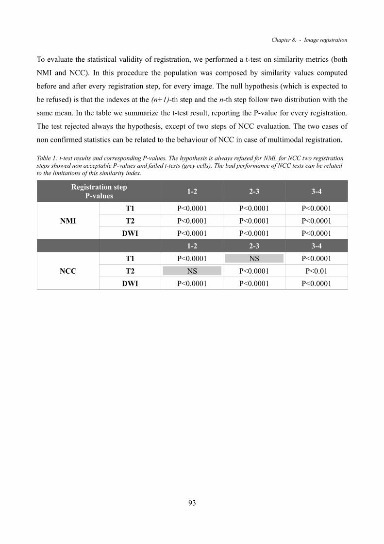
Chapter 8. - Image registration
To evaluate the statistical validity of registration, we performed a t-test on similarity metrics (both
NMI and NCC). In this procedure the population was composed by similarity values computed
before and after every registration step, for every image. The null hypothesis (which is expected to
be refused) is that the indexes at the (n+1)-th step and the n-th step follow two distribution with the
same mean. In the table we summarize the t-test result, reporting the P-value for every registration.
The test rejected always the hypothesis, except of two steps of NCC evaluation. The two cases of
non confirmed statistics can be related to the behaviour of NCC in case of multimodal registration.
Table 1: t-test results and corresponding P-values. The hypothesis is always refused for NMI, for NCC two registration steps showed non acceptable P-values and failed t-tests (grey cells). The bad performance of NCC tests can be related to the limitations of this similarity index.
Registration stepP-values
1-2 2-3 3-4
NMI
T1 P<0.0001 P<0.0001 P<0.0001
T2 P<0.0001 P<0.0001 P<0.0001
DWI P<0.0001 P<0.0001 P<0.0001
1-2 2-3 3-4
NCC
T1 P<0.0001 NS P<0.0001
T2 NS P<0.0001 P<0.01
DWI P<0.0001 P<0.0001 P<0.0001
93

Quantitative Characterization and Identification of Lymph Nodes and Nasopharingeal Carcinoma by Coregistered MR Images
8.2 Identification maps
The result of the identification procedure, based on templates collected by the radiologist, are two
maps, one derived from the main lesion data while the other from lymph nodes sampling. The maps
values are scaled to surely fit the range 0÷1000, their values are pure numbers as they are related to
the membership to the starting tissue template.
The anatomic features depicted are very few (lymph nodes and carcinoma), thus the spatial
collocation of those details is often not immediate. Numerical coordinates might be useful in such
conditions, but a better solution is to use maps as coloured layers over the T1-VIBE volume. This
volume, in fact, is widely used by physicians to investigate the anatomical detail (Figure 15).
Furthermore maps are already aligned to the coregistered image set. This makes possible to
visualize the superposition directly. Another salient feature is that the two maps (the one based on
carcinoma and the one based on lymph nodes) show a complementary behaviour. The lesion
94
Figure 15: Identification maps plotted over the anatomical T1 VIBE. The upper has been obtained starting from the lesion template, the lower is the result of the lymph nodes matching. The red arrows show the lymph nodes, the magenta the main lesion.

Chapter 8. - Identification maps
identification map shows a good performance in retrieving once again the lesion itself. It also shows
the capability of retrieving the peripheral area of the involved lymph nodes. An analogue behaviour
is found in the map defined by the lymph nodes template: lymph nodes cores are identified, but also
an area of the main lesion (Figure 15). Hence plotting both the maps together over T1-VIBE, with
two different colour scales can give all the informations in a single visualization (Figure 16).
In follow up exam sessions the represented tissues are the same: the residual lesion is retrieved both
by lesion and lymph nodes diagnostic templates; with dual behaviour the outer lymph nodes are
usually identified with lesion template while the inner zone is found using lymph nodes template.
Thus maps can be employed to perform comparisons between different examination sessions,
evaluating lymph nodes and carcinoma changes.
As visible in previous images (Figure 15, Figure 16) a significant amount of extraneous tissue
matches the lesion template, a more detailed analysis shows that the tissue depicted is mostly white
nervous matter, from spinal cord, brainstem, bulb, corpus callosum and cortex. It is worth to
remember that PET is subject of similar false positives, involving both white and grey matters, and
more in general tissues with high metabolic activity. Nevertheless the anatomic collocation and the
uniqueness of the structures makes them easy to identify and discard when the maps are analysed.
95
Figure 16: Identification maps represented over the T1 anatomical image. In hot colours the lesion template identification, in cold the lymph nodes template. The red arrows show the lymph nodes, the magenta the main lesion. As clearly visible informations given are complementary. This visualization appears extremely useful to detect the main carcinoma or lymph nodes size and location.

Quantitative Characterization and Identification of Lymph Nodes and Nasopharingeal Carcinoma by Coregistered MR Images
8.3 PET comparison
Where available (9 patients of 14) PET diagnosis images have been used to confirm the evidence of
lymph node and lesion location. The radiologist helped to identify the correct matches between
maps and PET. The first term of comparison was the number of detectable lymph nodes. Due to
limited PET resolution only lymph nodes wider than 5mm were considered on both PET images and
maps (Table 2). It is important to remember that maps have very higher resolution. This makes
possible to distinguish adjacent lymph nodes which in PET appear as an unique but larger lymph
node (Figure 17).
96
Figure 17: Identification maps (on the right) and PET (on the left). The blue arrows evidence a couple of lymph nodes which appear unique in PET. The red arrows point small lymph nodes not enhanced in PET.

Chapter 8. - PET comparison
No lymph node retrieved was without PET evidence, exception made for smaller one, which are too
small for that technique resolution (Figure 17). Globally much more lymph nodes can be identified
with the maps, but their dimensions are usually too small to be detected with PET. This comparison
produced the results summarized in the following tables (Table 3).
Table 2: Results for maps vs PET detected lymph nodes number. Only lymph nodes with Ø>5mm were considered
Patient Anon. Code 1 2 3 4 5 6 7 8 9 10 11 12 13 14 15
# of lymph nodes
PET 8 7 8 4 6 5 9 6 9
maps 13 7 16 8 9 8 12 11 9 5 5 11 12 12 9
97
Figure 18: 3D visualization of T1-VIBE volume, with lesion and lymph nodes based maps plotted respectively as hot and cold coloured layers. The magenta arrow points the main lesion, the red arrow a visible lymph node.

Quantitative Characterization and Identification of Lymph Nodes and Nasopharingeal Carcinoma by Coregistered MR Images
Table 3: Lymph nodes count in maps. Small lymph nodes are widely recognised
Patient Anon. Code 1 2 3 4 5 6 7 8 9 10 11 12 13 14 15
# of lymph nodes
Ø>5mm 13 7 16 8 9 8 12 11 9 5 5 11 12 12 9
Ø<5mm 7 5 >10 7 10 3 >10 >10 6 5 7 7 >10 8 5
Total 20 12 >26 15 19 11 >22 >21 15 10 12 18 >22 20 14
A similar task has been performed, looking at main carcinoma lesion. The area clearly identified by
maps as the main carcinoma was checked to be qualitative the same of PET. This task reported that
usually carcinomas shapes and locations in maps are coherent. Results are shown in table 4.
Table 4: Carcinoma identification summarizing table: C stand for coherent identification, 2 for two different carcinoma tissues with poor identification, R for relapse with non defined carcinoma boundaries and extended false positives.
Patient Anon. Code 1 2 3 4 5 6 7 8 9 10 11 12 13 14 15
Carcinoma identification
C C C 2 C C C C C C C C 2 C R
Exceptions have to be made in three clinical cases. Two of them were characterized by a
particularly developed carcinoma. Even from anatomical raw image appeared clearly that two
different tissues formed the main carcinoma lesion. The algorithm has been implemented on both
these tissues, but the resulting maps were clearly worse than the other, non defining clearly the
lesion boundaries. The last clinical case was a diagnosis of a so called relapse (carcinoma regrowth
after apparently successful treatments) treated by another clinic. The evidence showed that the
carcinoma, which appears to be homogeneous, can't be characterized effectively, resulting in a map
with several false positives and non defined lesion boundaries.
98

Chapter 8. - PET comparison
99

100

9.Conclusions
In this study were examined 15 patient subject of nasopharyngeal carcinoma (NPC) examined in
MR session, each composed by an anatomical T1-VIBE (with Gadolinium contrast), an axial T1
TSE, an axial T2 TSE and DW images for b-values 0,300,500,700,1000.
The DICOM images retrieved were reassembled spatially and resampled, with isotropic 0.5mm
resolution, to generate volumes. T1-VIBE volume was chosen as template and the other volumes
were registered on it. This multimodal procedure was performed by two multiresolution rigid
transformation, merging head and neck volumes, and a multiresolution non rigid transformation. We
obtain 8 fused volumes for each examination session.
Each patient volumes at diagnosis were used to perform a radiologist supervised location of tissue
of interest. Two main templates were located, the main carcinoma and the active lymph nodes
internal region. These templates were used to build a characterization of the tissue for each patient,
based images intensity.
Starting from the histograms of ROI volumes, it was possible to generate a 8-dimensional
membership function for each template, to perform a fuzzy-like approach for tissue identification.
The result of this procedure were two identification maps, with values normalized between 0 and
1000, completely overlapping the examination volumes.
The map based on main carcinoma sample detected the carcinoma itself with a good precision and
retrieved also the peripheral shell of the lymph nodes. The lymph nodes based identification map
evidences many lymph nodes and detected some regions of the main carcinoma too. Hence a
combined use of the maps is suggested, especially if depicted as two different coloured layers over
the anatomical volume.
101

Quantitative Characterization and Identification of Lymph Nodes and Nasopharingeal Carcinoma by Coregistered MR Images
These maps have the advantage to be already aligned and registered to the other image set.
Furthermore the obtained maps have a very higher resolution (isotropic 0.5mm). This allows a
better definition of pathological areas of interest, which is still a critical aspect in low resolution
imaging (such as PET or raw DWI or even ADC-maps).
Compared to PET examinations the identification maps showed good performance. The number of
lymph nodes retrieved (having Ø>5mm) in maps is equal or higher than PET. Their locations are the
same for both PET and maps, but the higher resolution of maps made possible to distinguish
adjacent lymph nodes. Further it was possible to identify many lymph nodes smaller than 5mm. The
main carcinoma region is clearly identified in most of cases and coherent with PET. If the disease is
in a very advanced status, different tissues may be present, thus boundary definition becomes
worse, as happened in two patients. In one patient the lesion identification was not possible, as the
carcinoma was a relapse. The false positive rate is comparable between these two techniques, even
if it seems to be lower in identification maps (no grey-matter false positives).
The follow up examination session were employed to define identification maps starting from
patient diagnostic ROIs. The results still presented the same behaviour. The identification of
interesting tissue appears better than PET imaging especially in residual carcinoma tissue or small
dimension lymph nodes.
This study shows how a MR examination composed with different contrast images (T1,T2,T1-Gd
and DWI) can collect many informations about the pathological course of NPC. Particular attention
should be given to the diffusive parameters of the tissues, which can give information about non-
physiological, especially too high, metabolism. The advantages of this technique are several: patient
does not suffer ionizing radiation exposure, the whole examination is taken in the same place, the
MRI costs are very lower than PET, the resolution of the resulting images is very higher.
However the results are preliminary and a clinical validation work is needed to give a quantitative
index of the reliability of this technique. An optimization work should be performed to improve
calculation time, which is still too high (more than two hours per session). An interesting
development could be to evaluate not only the average coefficient of diffusion, but to describe the
directionality of it, enabling a separation of directional highly diffusive tissues (white matter) from
non-directional highly diffusive ones (carcinoma).
The technique proposed in this study could be a new tool in NPC tissue identification and/or
evaluation. The maps can be used as an identification tool especially where the structures of interest
102

Chapter 9. - Conclusions
are small or their dimensions are diminish with therapy. Furthermore they can be a starting point for
the segmentation of interest areas and calculation of quantitative parameters (volume, mean ADC
etc.).
103

104

10. Acknowledgements
I want to personally thank:
Prof. L. Mainardi, for his kindness and open-minded interest to my thesis work;
Doc. P. Potepan, whose devotion to work is incredible, and willingness in tissue sampling has been
crucial;
Eng. E. Montin, for his trust in me and the every-day effort in tolerate my questions;
P. Lauricella, for helping me in many occasions, I'll help you back soon, be sure of it;
My family, who is supporting all my efforts, we are nearly done;
My friends, who understood and made me laugh when I needed to;
At last, but most of all, my darling Michela, for your love and your gentle smile, for your patience
and your tears, thanks for being so close to me in these years.
105

11. References
[1] : Chou J Lin Y C Kim J You L Xu Z He B Jablons D M, Nasopharyngeal carcinoma - Review of the molecolar mechanisms of tumorigenesis, Head & Neck: 30, 946-963 2008
[2] : Chenevert T. L., Principles of Diffusion-Weighted Imaging (DW-MRI) as Applied to Body Imaging in Diffusion-Weighted MR Imaging Springer Berlin Heidelberg 1 3-17 2010
[3] : Bloch F, Nuclear Induction, Phys Rev: 70, 460 1946
[4] : Purcell E.M. Torrey H. C. Pound R.V., Resonance absorption by nuclear moments in a solid, Phys Rev: 69, 37 1946
[5] : Ernst R.R. Anderson W.A., Application of Fourier transform spectroscopy to magnetic resonance, Rev Sci Instrum: 37, 93 1966
[6] : Lauterbur P. C., Image formation by induced local interactions: examples employing nuclear magnetic resonance, Nature: 242, 190-191 1973
[7] : G. Valli G. Coppini Bioimmagini. Pàtron Editore 2005
[8] : Landini L Multimodal approach to human brain function assessment. Pisa University Press 2009
[9] : Crank J. The mathematics of diffusion. Oxford University Press 1975
[10] : Szafer A. Zhong J. Gore J.C., Theoretical model for water diffusion in tissues, Magn Reson Med: 33, 697-712 1995
[11] : Haacke E. M. Brown R.W. Thompson M.R. et al Magnetic resonance imaging: physucal principles and sequence design.. John Wiley 1999
[12] : Stejskal E.O. Tanner J.E., Spin diffusion measurements: spin echoes in the presence of a time-dependent field gradient, J Chem Phys: 42, 288-292 1965
[13] : Le Bihan D. Breton E. Lallemand D. et al, MR imaging of intravoxel incoherent motions: application to diffusion and perfusion in neurologic disorders, Radiology: 161, 401-407 1986
[14] : Le Bihan D. Mangin JF, Poupon C. et al, Diffusion tensor imaging: concepts and applications, J Magn Reson Imaging: 13, 534-546 2001
106

Chapter 11. - References
[15] : Da Xinga, Nikolaos G. Papadakisa, Christopher L. -H. Huangb, Vee Meng Leea, T. Adrian Carpentera and Laurance D. Hall, Optimised diffusion-weighting for measurement of apparent diffusion coefficient (ADC) in human brain, Magn. Reson. Med.: 7, 771-784 1997
[16] : D. Rueckert, L. I. Sonoda, C. Hayes, D. L. G. Hill, M. O. Leach, and D. J. Hawkes., Non-rigid registration using Free-Form Deformations: Application to breast MR images., IEEETransactions on Medical Imaging: , 712-721 1999
[17] : D. L. G. Hill, P. G. Batchelor, M. Holden and D. J. Hawkes, Medical image registration, Phys. Med. Biol.: 46, 1-45 2001
[18] : Maintz J B Viergever M A, A survey of medical image registration in Medical Image Analisys 2 1-36 1998
[19] : Van Den Elsen P A Pol E J D Viergever M, Medical Image matching - A review with classification, IEEE Engineering in Medicine and Biology: 12, 26-39 1993
[20] : Press W Teukolsky S Vetterling W T Flannery B P, Numerical recipes in C++ - The art of scientific computing, Cambridge University: , 2002
[21] : Maes F Collignon A Vandenmeulen D Suetens P, comparative evaluation of multiresolution optimization strategies for multimodality image registratation by maximization of mutual information in Medical Image Analisys 3 373-386 1999
[22] : Positano V, Image registration methods in MRI in Advanced imaging processing in Magnetic Resonance Imaging 27 189-222 2005
[23] : De Castro E Morandi C, Registration of translated and rotated images using finite Fourier transforms, IEEE Transaction on Pattern analisys and Machine Intelligence: 9, 700-703 1987
[24] : Lehmann L Goerke C Schmitt W Kaupp A Repges R, A rotation-extended chepstrum technique optimized by systematic analisys of various sets of X-ray images in Medical Imaging: Image Processing 390-401 1996
[25] : Maes F Collignon A Vandermeulen D Marchal G Suetens P, Multimodality image registration by maximization of mutual information, IEEE Transaction on Medical Imaging: 16, 187-198 1997
[26] : Wells W M Viola P Atsumi H Nakajima S Kikinis R, Multi-modal volume registration by maximization of mutual information in Medical Image Analisys 1 35-51 1996
[27] : Pluim J Maintz J Viergever M, Mutual-information-based registration of medial images: a survey, IEEE Transaction on Medical Imaging: 22, 986-1004 2003
[28] : Collignon A Vandermeulen D suetens P Marchal G, 3D multimodality medical image registration using feature space clustering in Computer vision, Virtual reality and Robotics in Medicine 195-204 1995
[29] : Studholme C Hill D Hawkes D, Multiresolution voxel similarity measueres for MR-PET registration in Information Processing in Medical Imaging 287-298 1995
[30] : Hill D Hawkes D Harrison N Ruff C, A strategy for automated multimodality image registration incorporating anatomical knowledge and imager characteristics in Information processing in medical imaging 182-196 1993
[31] : Collignon A Maes F Delaere D Vandermeulen D Suetens P Marchal G, Automated multimodality image registration based on information theory in Information Processing in Medical Imaging 263-274 1995
[32] : Viola P Wells M, Alignment by maximization of mutual information in International Conference on Computer Vision 16-23 1995
[33] : J. A. Schnabel, D. Rueckert, et Al., A Generic Framework for Non-Rigid Registration Basedon Non-Uniform Multi-Level Free-Form Deformations, In Fourth Int. Conf. on Medical Image Computing and Computer-Assisted Intervention (MICCAI '01): , 573-581 2001
107

Quantitative Characterization and Identification of Lymph Nodes and Nasopharingeal Carcinoma by Coregistered MR Images
[34] : Dlgs 196/2003.
[35] : The MathWorks Inc., Interpolating Scattered Data Using theTriScatteredInterp Class in Matlab 2010 Help Guide 7 19-32
[36] : Golias N A Dutton R W, Delaunay triangulation and 3D adaptative mesh generation, Finite Elements in Analysis and Design: 25, 331-341 1997
[37] : Neuroimaging Informatic Technology Initiative, http://nifti.nimh.nih.gov/, 2005
108