quantitative analysis · - venn diagram probability theory and distribution probability theory -...
TRANSCRIPT

QUANTITATIVE ANALYSIS
CPA
CCP
CIFA
PART II
Section 4
STUDY TEXT
KASNEB JULY 2018 SYLLABUS
Revised on: January 2019
Somea
Kenya
- Sam
ple n
otes
0707
737
890

QUANTITATIVE ANALYSIS
www.someakenya.co.ke Contact: 0707 737 890 Page 2
CONTENT 1. Basic mathematical techniques Functions
- Functions, equations and graphs: Linear, quadratic, cubic, exponential and logarithmic - Application of mathematical functions in solving business problems
Matrix algebra
- Types and operations (addition, subtraction, multiplication, transposition, and inversion) - Application of matrices: statistical modelling, Markov analysis, input- output analysis
and general applications
Calculus - Differentiation
• Rules of differentiation (general rule, chain, product, quotient) • Differentiation of exponential and logarithmic functions • Higher order derivatives: Turning points (maxima and minima) • Ordinary derivatives and their applications • Partial derivatives and their applications • Constrained Optimisation; lagrangian multiplier
- Integration
• Rules of integration • Applications of integration to business problems
2. Probability
Set theory - Types of sets - Set description: Enumeration and descriptive properties of sets - Operations of sets: Union, intersection, complement and difference - Venn diagram
Probability theory and distribution Probability theory - Definitions: Event, outcome, experiment, sample space - Types of events: Elementary, compound, dependent, independent, mutually exclusive,
exhaustive, mutually inclusive - Laws of probability: Additive and multiplicative rules - Baye's Theorem - Probability trees - Expected value, variance, standard deviation and coefficient of variation using
frequency and probability
Probability distributions - Discrete and continuous probability distributions (uniform, normal, binomial, poisson
and exponential) - Application of probability to business problems
Somea
Kenya
- Sam
ple n
otes
0707
737
890

QUANTITATIVE ANALYSIS
www.someakenya.co.ke Contact: 0707 737 890 Page 3
3. Hypothesis testing and estimation
- Hypothesis tests on the mean (when population standard deviation is unknown) - Hypothesis tests on proportions - Hypothesis tests on the difference between means (independent samples) - Hypothesis tests on the difference between means (matched pairs) - Hypothesis tests on the difference between two proportions
4. Correlation and regression analysis
Correlation analysis • Scatter diagrams • Measures of correlation -product moment and rank correlation coefficients (Pearson
and Spearman) Regression analysis • Assumptions of linear regression analysis • Coefficient of determination, standard error of the estimate, standard error of the
slope, t and F statistics • Computer output of linear regression • T-ratios and confidence interval of the coefficients • Analysis of Variances (ANOVA) • Simple and multiple linear regression analysis
5. Time series
- Definition of time series - Components of time series (circular, seasonal, cyclical, irregular/ random, trend) - Application of time series - Methods of fitting trend: free hand, semi-averages, moving averages, least squares
methods - Models- additive and multiplicative models - Measurement of seasonal variation using additive and multiplicative models - Forecasting time series value using moving averages, ordinary least squares method and
exponential smoothing - Comparison and application of forecasts for different techniques
6. Linear programming
- Definition of decision variables, objective function and constraints - Assumptions of linear programming - Solving linear programming using graphical method - Solving linear programming using simplex method - Sensitivity analysis and economic meaning of shadow prices in business situations - Interpretation of computer assisted solutions - Transportation and assignment problems
7. Decision theory
- Decision process
Somea
Kenya
- Sam
ple n
otes
0707
737
890

QUANTITATIVE ANALYSIS
www.someakenya.co.ke Contact: 0707 737 890 Page 4
- Decision making environment - deterministic situation (certainty), analytical hierarchical approach (AHA), risk and uncertainty, stochastic situations (risk), situations of uncertainty
- Decision making under uncertainty - maximin, maximax, minimax regret, Hurwicz decision rule, Laplace decision rule
- Decision making under risk - expected monetary value, expected opportunity loss, minimising risk using coefficient of variation, expected value of perfect information
- Decision trees - sequential decision, expected value of sample information - Limitations of expected monetary value criteria
8. Game theory
- Assumptions of game theory - Zero sum games - Pure strategy games (saddle point) - Mixed strategy games (joint probability approach) - Dominance, graphical reduction of a game - Value of the game. - Non zero sum games - Limitations of game theory
9. Network planning and analysis
- Basic concepts - network, activity, event - Activity sequencing and network diagram - Critical path analysis (CPA) - Float and its importance - Crashing of activity/project completion time - Project evaluation and review technique (PERT) - Resource scheduling (levelling) and Gantt charts - Limitations and advantages of CPA and PERT
10. Queuing theory
- Components/elements of a queue: arrival rate, service rate, departure, customer behaviour, service discipline,' finite and infinite queues, traffic intensity
- Elementary single server queuing systems - Finite capacity queuing systems - Multiple server queues
11. Simulation
- Types of simulation - Variables in a simulation model - Construction of a simulation model - Monte Carlo simulation - Random numbers selection - Simple queuing simulation: Single server, single channel "first come first served"
(FCFS) model - Application of simulation models
Somea
Kenya
- Sam
ple n
otes
0707
737
890

QUANTITATIVE ANALYSIS
www.someakenya.co.ke Contact: 0707 737 890 Page 5
CONTENT PAGE Topic 1: Basic mathematical techniques……………………………………………… …..…6 Topic 2: Probability………………………………………………………………………….100 Topic 3: Hypothesis testing and estimation…………………………………………………151 Topic 4: Correlation and regression analysis…………………………………………….….162 Topic 5: Time series……………………………………………………………………..…..199 Topic 6: Linear programming………………………………………………………………..227 Topic 7: Decision theory………………………………………………………………..……280 Topic 8: Game theory………………………………………………………...……………...301 Topic 9: Network planning and analysis………………………………………… ….……..310 Topic 10: Queuing theory………………………………………………...…………..….…..330 Topic 11: Simulation…………………………………………………...……………….……345 Topic 12: Emerging issues and trends
Somea
Kenya
- Sam
ple n
otes
0707
737
890

QUANTITATIVE ANALYSIS
www.someakenya.co.ke Contact: 0707 737 890 Page 6
TOPIC 1
BASIC MATHEMATICAL TECHNIQUES
FUNCTIONS
Definitions
1. Variables
A variable is any quantity that assumes different values in a particular analysis.
Examples
i. Production costs
ii. Material costs
iii. Sales revenue
2. Constant
This is any quantity whose value remains unchanged in a particular analysis.
Examples
Fixed costs
Rents
Tuition fees
Note: In a given analysis there are two types of variables namely:
i. Independent variable/predictor variable
ii. Dependent / response variable
Independent variable is that which influences the value of the other variables in a particular
analysis.
Dependent variable isthat whose value is influenced or changes when the value of other
variables (independent) changes.
3. Functions
A function is a mathematical expression which describes a relationship between two or more
variables in a particular analysis specifically one dependant variable and one or more
independent variables.
Examples
If the price of the consumer product is Sh 40 per Kg, then the total sales revenue, S when Q
units of the products are produced and sold is obtained as follows:
Somea
Kenya
- Sam
ple n
otes
0707
737
890

QUANTITATIVE ANALYSIS
www.someakenya.co.ke Contact: 0707 737 890 Page 7
S = 40q
In this case S is the dependent variable, q the independent variable and 40 is a constant.
In terms of number of variables in a function, functions can be classified into the following
categories:
i. Univariate function
ii. Bivariate function
iii. Multivariate function
A univariate function is that which involves two variables only, one dependent variable and
one independent and is generally written as:
y = f (x) where y = dependent variable
x = independent variable
and f(x) = Function of x
Example of univariate function
The price of a house is dependent among other factors, on the size of the house. In functional
form, this could be written as follows:
Price = f (size)
Where price is dependent variable
Size is independent variable
A Bivariate function is that which involves three variables only, one dependent variable and
two independent variables:
Example
A student’s performance or grade in an examination could be dependent upon the following
factors
i) IQ
ii) Time spent on studying in terms of Hours, H
In functional form, this is written as follows:
Grade = f (IQ,H)
Grade is dependent variables
IQ, H Are independent variables
Multivariable function is that function which involves four or more variables, one dependent
variable and three or more independent variables.
Example
The price of a house depends on the following factors:
i) Size
ii) Location
Somea
Kenya
- Sam
ple n
otes
0707
737
890

QUANTITATIVE ANALYSIS
www.someakenya.co.ke Contact: 0707 737 890 Page 8
iii) Security
iv) Nature of the house
In functional form this is written as follows;
Price = f (size, location, security, nature of the house)
Where price – is dependent variable
Size, location, security, nature of the house are independent variables.
Graph of a function
A graph is a visual method of illustrating the behaviour of a particular function. It is easy to see
from a graph how as x changes, the value of f(x) is changing.
The graph is thus much easier to understand and interpret than a table of values. For example
by looking at a graph we can tell whether f(x) is increasing or decreasing as x increases or
decreases.
We can also tell whether the rate of change is slow or fast. Maximum and minimum values of
the function can be seen at a glance. For particular values of x, it is easy to read the values of
f(x) and vice versa i.e. graphs can be used for estimation purposes
Different functions create different shaped graphs and it is useful knowing the shapes of some
of the most commonly encountered functions. Various types of equations such as linear,
quadratic, trigonometric, exponential equations can be solved using graphical methods.
TYPES OF FUNCTIONS IN BUSINESS
These include
1. Linear functions
2. Quadratic functions. Polynominals
3. Cubic functions
4. Exponential functions
5. Logarithmic functions
6. Hybrid functions
1. Linear functions
A linear function is a first degree polynomial function that takes the following general form.
y= a +bx
Where y is dependent variable
x is independent variable
a is y-intercept or the value of y when x = 0
b is the slope or gradient or the amount by which y changes in value when x changes by a unit
Somea
Kenya
- Sam
ple n
otes
0707
737
890

QUANTITATIVE ANALYSIS
www.someakenya.co.ke Contact: 0707 737 890 Page 9
Properties/characteristics of linear functions
When plotted on an x-y coordinate system, the result is a straight line whose general direction
is dependent on the slope, b of the function.
Specifically, if
a) Slope, b > 0 (+ve)
b) Slope, b < 0 (negative)
c) Slope, b = 0
d) Slope, b is undefined or b = ∞
Y = a + bx
X
Y
a
y = a - bx
X
Y
a
a/b
y = a
x
y
a
x
y
Somea
Kenya
- Sam
ple n
otes
0707
737
890

QUANTITATIVE ANALYSIS
www.someakenya.co.ke Contact: 0707 737 890 Page 10
2. A linear equation has only one root or solution
3. A linear function is completely specified if either
a) Two points or
b) One point and the slope of the function are given.
ILLUSTRATIONS
Properties of linear functions or equations
1. Find the equation of the straight line which passes through the two point given as :
When x = 1, y = 8
x = -2, y = 4
2. Find the expression for the linear function which passes through the two points given as:
(x,y) = (1,1)
(x,y) = (-2,6)
3. Find the equation of the straight line with a slope of -5 which passes through the point (3,5)
SOLUTIONS
1. Let the linear equation be y = a +bx
i) 8 = a + b 8 = a + b (i)
ii) 4 = a + -2b 4= a – 2b (ii)
4 = a =2b 4 = 3b b = 4/3
Substitute b in (i) 8 = a +�
�
a = �
�−
�
� =
����
�=
��
�
Hence the equation of the straight line is:
y =��
�−
�
� x
3y = 20 + 4x
2. Let the linear equation be y = a + bx
Let the linear equation be y = a+bx
1 = a+b............. (i)
� ������
�����∴ b = −5
3�
1 = a − 53�
a = �
�+
�
� =
���
�=
�
�
∴ The equation will be
y = �
�−
� �
�
Somea
Kenya
- Sam
ple n
otes
0707
737
890

This is a SAMPLE (Few pages extracted from the complete notes: Page
numbers reflects the original pages on the complete notes).
It’s meant to show you the topics covered in the notes.
Download more at our websites:
www.someakenya.co.ke or
www.someakenya.com
To get the complete notes either in softcopy form or in
Hardcopy (printed & Binded) form, contact us:
Call/text/whatsApp 0707 737 890
Email: [email protected]
Get news and updates about kasneb by liking our page
www.fb.com/studycpa
Or following us on twitter www.twitter.com/someakenya
Pass on first attempt
“Buy quality notes and avoid refers/retakes which costs more money and time”
Sample/preview is NOT FOR SALE
Somea
Kenya
- Sam
ple n
otes
0707
737
890

QUANTITATIVE ANALYSIS
www.someakenya.co.ke Contact: 0707 737 890 Page 88
REVISION EXERCISES
QUESTION 1
Demand function for a firm is given by QP 4.012
P is the price of the product, Q is the quantity demanded, and the total cost (C) is given by
26.045 QQC
At what price and quantity will the firm have maximum profit? If the firm aims at maximizing
sales, what price should it charge?
Solution:
Let profit = z
Profit z = PQ – C
= (12 – 0.4Q) Q – (5 + 4Q + 0.6Q2)
= 12Q – 0.4Q2 – 5 – 4Q – 0.6Q2
= 8Q – Q2 – 5
For maximum profit, the differentiation of z with respect to Q equals zero.
0Q28dQ
dz 2Q = 8 Q = 4
So P = 12 – 0.4Q and for Q =4
= 12 – 1.6
= 10.4
2
2
dQ
zd= - 2 Q 0 Profit is maximized.
Profit is maximised at a price of 10.4 and when quantity = 4
To maximize sales then,
0)4.012()( 2
dQ
QQd
dQ
PQd
= 12 – 0.8Q = 0
Q = 8.0
12= 15 and since 08.0
dQ
)PQ(d2
2
then sales is maximized
So P = 12 – 0.4 15
= 6
Somea
Kenya
- Sam
ple n
otes
0707
737
890

QUANTITATIVE ANALYSIS
www.someakenya.co.ke Contact: 0707 737 890 Page 89
QUESTION 2
a) Two CPA students were discussing the relationship between average cost and total cost.
One student said that since average cost is obtained by dividing the cost function by the
number of units Q, it follows that the derivative of the average cost is the same as marginal
cost, since the derivative of Q is 1.
Required:
Comment on this analysis.
b) Gatheru and Kabiru Certified Public Accountants have recently started to give business
advise to their clients. Acting as consultants, they have estimated the demand curve of a
clients firm to be;
AR=200-8Q
Where AR is average revenue in millions of shillings and Q is the output in units.
Investigation of the client firm’s cost profile shows that marginal cost (MC) is given by:
MC=Q2-28Q+211(In million shillings)
Further investigations have shown that the firm’s cost when not producing output is sh.10
million.
Required:
i) The equation of total cost
ii) The equation of total revenue
iii) An expression for profit.
iv) The level of output that maximizes profit
v) The equation of marginal revenue.
Solution:
a) Taking the following to mean:
TC – Total cost
AC – Average cost
MC – Marginal cost
Q – Number of units
Then AC = Q
TC
And MC = dQ
)TC(d
These are the relationships that link TC, AC, and MC.
To comment on the CPA students analysis,
Somea
Kenya
- Sam
ple n
otes
0707
737
890

This is a SAMPLE (Few pages extracted from the complete notes: Page
numbers reflects the original pages on the complete notes).
It’s meant to show you the topics covered in the notes.
Download more at our websites:
www.someakenya.co.ke or
www.someakenya.com
To get the complete notes either in softcopy form or in
Hardcopy (printed & Binded) form, contact us:
Call/text/whatsApp 0707 737 890
Email: [email protected]
Get news and updates about kasneb by liking our page
www.fb.com/studycpa
Or following us on twitter www.twitter.com/someakenya
Pass on first attempt
“Buy quality notes and avoid refers/retakes which costs more money and time”
Sample/preview is NOT FOR SALE
Somea
Kenya
- Sam
ple n
otes
0707
737
890

QUANTITATIVE ANALYSIS
www.someakenya.co.ke Contact: 0707 737 890 Page 100
TOPIC 2
PROBABILITY THEORY
SET THEORY
A Set is a collection of distinct items or objects e.g. members, letters, people, houses etc.
The items or objects in a set are called members or elements of the set.
Any set is denoted using a capital letter while the elements are denoted using small letters.
The members or elements of the set are enclosed within the curly brackets and separated using
comas, e.g. a set of vowels can be written as follows; A = {a, e, i, o, u}
If element x is a member of set A it is denoted as follows
x ∈ A (x belongs to set A)
If X is not an element of A it is denoted as
� ∉A (x doesn’t belong to set A)
We may consider all the ocean in the world to be a set with the objects being whales, sea
plants, sharks, octopus etc, similarly all the fresh water lakes in Africa can form a set.
Supposing A to be a set
A = {4, 6, 8, 13}
The objects in the set, that is, the integers 4, 6, 8 and 13 are referred to as the members or
elements of the set. The elements of a set can be listed in any order. For example,
A = {4, 6, 8, 13} = {8, 4, 13, 6}
Sets are always precisely defined. Each element occurs once and only once in a set.
The notation is used to indicate membership of a set. ∉ represents non membership.
However, in order to represent the fact that one set is a subject of another set, we use the
notation . A set “S” is a subset of another set “T” if every element in “S” is a member of “T”
Example
If A = {4, 6, 8, 13} then
i) 4 {4, 6, 8, 13} or 4 A; 16 ∉ A
ii) {4, 8} A; {5, 7} A; A A
Methods of set representation
Capital letters are normally used to represent sets. However, there are two different methods
for representing members of a set:
i. The descriptive method and
Somea
Kenya
- Sam
ple n
otes
0707
737
890

QUANTITATIVE ANALYSIS
www.someakenya.co.ke Contact: 0707 737 890 Page 101
ii. The enumerative method
The descriptive method involves the description of members of the set in such a way that one
can determine the elements of the set without difficulty.
The enumerative method requires that one writes out all the members of the set within the
curly brackets.
For example, the set of numbers 0, 1, 2, 3, 4, 5, 6 and 7 can be represented as follows
P = {0, 1, 2, 3, 4, 5, 6, 7} , enumerative method
P = {X/x = 0, 1, 2…7} descriptive method
Or
P = {x/0 ≤ x ≤7} where x is an integer.
Application of set Theory
i) It is used in capturing statistical data.
ii) It is used in solving counting problems
iii) It shows the logical relationship between two or more sets.
iv) It creates a basis for probability theory
v) It is a research tool that can be used in data capturing.
TYPES OF SETS
Subset – This is a portion of a set where the elements of that set belongs to another bigger set.
Universal set (U) – This is a set containing all the elements under consideration e.g. a set of all
the students in college, a set of alphabetical letters, a set of all the months in the source of the
year.
Finite set – This is a set containing countable elements e.g. a set of weekdays a set of students
in sec iv etc.
Null/Empty /void set (∅) – A set without elements, e.g. a set of married bachelors.
Infinite sets – This is a set containing countless elements e.g. a set of counting numbers.
Sets concepts and Operations
Concepts;
1. Overlapping sets
These are two or more sets with some common elements.
Eg: A{1,2,3,4,5,6}
B{2,4,6,8,10} Overlapping set.
2. Sets equality
Somea
Kenya
- Sam
ple n
otes
0707
737
890

QUANTITATIVE ANALYSIS
www.someakenya.co.ke Contact: 0707 737 890 Page 102
Two or more sets are said to be equal if and only if they have the same elements but not
necessarily the same order of elements.
Eg: A- {a, b, c, d}
C = {b,c, a, d,}
A = C
3. Disjoint sets
These are two or more sets without common elements
Eg: A- {a, b, c, d}
C = {1,2, 3, 4,}
Set operation;
1) Sets intersection (n)
This operation represents a set containing the common elements in two or more sets.
If A = {1 2 3 4 5 6}
B = {2, 4, 6, 8, 10}
Then AnB = {2 4 6}
If set C = {11, 12, 13,14}
Then AnC =(∅)
2) Set Union
This operation represents a collection of all the elements in two or more sets without
repetition if the sets are overlapping.
If A = {1 2 3 4 5 6} ⟹ n (A) = 6
B = { 2, 4, 6, 8, 10}⟹n (B) = 5
AUB = {1, 2, 3, 4, 5, 6, 8, 10} ⟹ n(AUB) = 8
3) Set difference (-)
Given two sets A & B which are overlapping, the difference between A & B is a set of
elements that are in set A but not in set B.
Similarly B difference A is a set of elements in B but not in A.
If A = {1, 2, 3, 4, 5, 6}
B= {2, 4, 6, 8, 10}
Then A – B = {1, 3, 5}
B – A = {8, 10}
4) Compliment (C)
Compliment of a set is a set of elements that are not in the original set but they are part of
the universal set, e.g.
If A = {1, 2, 3, 4, 5, 6}
Then compliment of A = Ac = A1 = {7, 8, 9, 10 .........∝ }
Somea
Kenya
- Sam
ple n
otes
0707
737
890

QUANTITATIVE ANALYSIS
www.someakenya.co.ke Contact: 0707 737 890 Page 103
NB//
Set theory begins with a fundamental binary relation between an object o and a set A. If o is a member (or element) of A, write o∈A. Since sets are objects, the membership relation can relate sets as well.
A derived binary relation between two sets is the subset relation, also called set inclusion. If all the members of set A are also members of set B, then A is a subset of B, denoted A⊆B. For example, {1, 2} is a subset of {1,2,3} , but {1,4} is not. From this definition, it is clear that a set is a subset of itself; for cases where one wishes to rule out this, the term proper subset is defined. A is called a proper subset of B if and only if A is a subset of B, but B is not a subset of A.
Just as arithmetic features binary operations on numbers, set theory features binary operations on sets. The: Union of the sets A and B, denoted A∪B, is the set of all objects that are a member of A,
or B, or both. The union of {1, 2, 3} and {2, 3, 4} is the set {1, 2, 3, 4} . Intersection of the sets A and B, denoted A ∩ B, is the set of all objects that are members
of both A and B. The intersection of {1, 2, 3} and {2, 3, 4} is the set {2, 3} . Set difference of U and A, denoted U \ A, is the set of all members of U that are not
members of A. The set difference {1,2,3} \ {2,3,4} is {1} , while, conversely, the set difference {2,3,4} \ {1,2,3} is {4} . When A is a subset of U, the set difference U \ A is also called the complement of A in U. In this case, if the choice of U is clear from the context, the notation Ac is sometimes used instead of U \ A, particularly if U is a universal set as in the study of Venn diagrams.
Symmetric difference of sets A and B, denoted A△B or A⊖B, is the set of all objects that are a member of exactly one of A and B (elements which are in one of the sets, but not in both). For instance, for the sets {1,2,3} and {2,3,4} , the symmetric difference set is {1,4} . It is the set difference of the union and the intersection, (A∪B) \ (A ∩ B) or (A \ B) ∪ (B \ A).
Cartesian product of A and B, denoted A × B, is the set whose members are all possible ordered pairs (a,b) where a is a member of A and b is a member of B. The cartesian product of {1, 2} and {red, white} is {(1, red), (1, white), (2, red), (2, white)}.
Power set of a set A is the set whose members are all possible subsets of A. For example, the power set of {1, 2} is { {}, {1}, {2}, {1,2} } .
Some basic sets of central importance are the empty set (the unique set containing no elements), the set of natural numbers, and the set of real numbers.
Somea
Kenya
- Sam
ple n
otes
0707
737
890

QUANTITATIVE ANALYSIS
www.someakenya.co.ke Contact: 0707 737 890 Page 104
VENN DIAGRAMS
This is a pictorial representation of sets and their relationships.
They involve the use of loops enclosed within a square or a rectangle. The loop represent a
specific set while the square / rectangle represents the universal set from where the set was
drawn.
If set B is a subset of A then the venn diagram of subset B is (BCA).
Set A
Intersection of set A & B (AnB) (overlapping sets)
IF A = {1, 2, 3, 4 ,5, 6}
B= {2, 4, 6, 8, 10}
Then;
AUB (A union B) (Overlapping sets)
A B
�
�
AnB
1 3
5
2 4 6
8 10
Somea
Kenya
- Sam
ple n
otes
0707
737
890

This is a SAMPLE (Few pages extracted from the complete notes: Page
numbers reflects the original pages on the complete notes).
It’s meant to show you the topics covered in the notes.
Download more at our websites:
www.someakenya.co.ke or
www.someakenya.com
To get the complete notes either in softcopy form or in
Hardcopy (printed & Binded) form, contact us:
Call/text/whatsApp 0707 737 890
Email: [email protected]
Get news and updates about kasneb by liking our page
www.fb.com/studycpa
Or following us on twitter www.twitter.com/someakenya
Pass on first attempt
“Buy quality notes and avoid refers/retakes which costs more money and time”
Sample/preview is NOT FOR SALE
Somea
Kenya
- Sam
ple n
otes
0707
737
890

QUANTITATIVE ANALYSIS
www.someakenya.co.ke Contact: 0707 737 890 Page 140
REVISION EXERCISES
QUESTION 1
A problem is given to three managers A, B, C whose chances of solving are ½, ⅓, ¼
respectively. What is the probability that the problem will be solved?
Solution:
The product of the probabilities of each manager solving a problem gives probability of
solving a problem. (Since one manager solving a problem is independent of the others)
P (solving)= 1- P (not solving)
= 1- ��
�x
�
�x
�
�� = 1 −
�
�=
�
�
QUESTION 2
Three groups of children contain respectively 3 girls and 1 boy; 2 girls and 2 boys; 1girl and 3
boys. One child is selected at random from each group, show that the chance that the three
selected, consist of 1 girl and 2 boys is 13/32.
Solution:
The best way to solve this is by use of a probability tree as follows:
Let G be the event of a girl being chosen
And B be the event of a boy being chosen
G 3/4
G 1/2
G 1/4
G 1/4
G 1/2
G 1/4
G 1/4
B 1/4
B 3/4
B 1/2
B 3/4
B 3/4
B 1/2
B 3/4
BBB
GGG
GGB
GBG
GBB
BGG
BGB
BBG
¾ ½ ¾
¼ ½ ¾
¼ ½ ¼
9/32
3/32
1/32
Group1
Group3
Group2 Som
eaKen
ya -
Sample
not
es
0707
737
890

QUANTITATIVE ANALYSIS
www.someakenya.co.ke Contact: 0707 737 890 Page 141
Sum of the required probabilities gives the following.
P (GBB) + P(BGB) + P(BBG)
�
�x
�
�x
�
� +
�
�x
�
�x
�
� +
�
�x
�
�x
�
�
3213
321
323
329P
QUESTION 3
The following table gives a bi-variate frequency distribution of 50 managers according to their
age and salary (in rupees).
Salary in rupees
Age in
years
1000-1500 1500-2000 2000-2500 2500-3000 Total
20-30 2 3 - - 5
30-40 5 4 2 1 12
40-50 - 2 10 3 15
50-60 - 1 8 9 18
Total 7 10 20 13 50
If a manager is chosen at random from the above distribution, find the chance that; (i) he is in
the age group of 30-40 and earns more than Rs.1500, (ii) his earnings are in the range of
Rs.2000-2500 and is less than 50 years old.
Solution:
i) Let A be the age group 30-40
B be the earnings more than 1500
Then P (B/A) = 12
7
5012
507
AP
ABP Then the probability of B given A
Where: P (AB) - Probability of A and B occurring.
P (A) - Probability of A occurring.
ii) Let A be the age group below 50 years
B be the earnings varying between 2000-2500
Then P (B/A) = 20
12
5020
5012
AP
ABP
QUESTION 4
Computer analysis of satellite data has correctly forecast locations of economic oil deposits
80% of the time. The last 24 oil wells drilled produced only 8 wells that were economic. The
Somea
Kenya
- Sam
ple n
otes
0707
737
890

This is a SAMPLE (Few pages extracted from the complete notes: Page
numbers reflects the original pages on the complete notes).
It’s meant to show you the topics covered in the notes.
Download more at our websites:
www.someakenya.co.ke or
www.someakenya.com
To get the complete notes either in softcopy form or in
Hardcopy (printed & Binded) form, contact us:
Call/text/whatsApp 0707 737 890
Email: [email protected]
Get news and updates about kasneb by liking our page
www.fb.com/studycpa
Or following us on twitter www.twitter.com/someakenya
Pass on first attempt
“Buy quality notes and avoid refers/retakes which costs more money and time”
Sample/preview is NOT FOR SALE
Somea
Kenya
- Sam
ple n
otes
0707
737
890

QUANTITATIVE ANALYSIS
www.someakenya.co.ke Contact: 0707 737 890 Page 151
TOPIC 3
HYPOTHESIS TESTING AND ESTIMATION
Meaning of Hypothesis Testing
A statistical hypothesis is an assumption about a population parameter. This assumption may or may not be true. Hypothesis testing refers to the formal procedures used by statisticians to accept or reject statistical hypotheses.
Statistical Hypotheses
The best way to determine whether a statistical hypothesis is true would be to examine the entire population. Since that is often impractical, researchers typically examine a random sample from the population. If sample data are not consistent with the statistical hypothesis, the hypothesis is rejected.
There are two types of statistical hypotheses.
Null hypothesis. The null hypothesis, denoted by H0, is usually the hypothesis that sample observations result purely from chance.
Alternative hypothesis. The alternative hypothesis, denoted by H1 or Ha, is the hypothesis that sample observations are influenced by some non-random cause.
For example, suppose we wanted to determine whether a coin was fair and balanced. A null hypothesis might be that half the flips would result in Heads and half, in Tails. The alternative hypothesis might be that the number of Heads and Tails would be very different. Symbolically, these hypotheses would be expressed as
H0: P = 0.5 Ha: P ≠ 0.5
Suppose we flipped the coin 50 times, resulting in 40 Heads and 10 Tails. Given this result, we would be inclined to reject the null hypothesis. We would conclude, based on the evidence, that the coin was probably not fair and balanced.
Hypothesis Tests
Statisticians follow a formal process to determine whether to reject a null hypothesis, based on sample data. This process, called hypothesis testing, consists of four steps.
State the hypotheses. This involves stating the null and alternative hypotheses. The hypotheses are stated in such a way that they are mutually exclusive. That is, if one is true, the other must be false.
Somea
Kenya
- Sam
ple n
otes
0707
737
890

QUANTITATIVE ANALYSIS
www.someakenya.co.ke Contact: 0707 737 890 Page 152
Formulate an analysis plan. The analysis plan describes how to use sample data to evaluate the null hypothesis. The evaluation often focuses around a single test statistic.
Analyze sample data. Find the value of the test statistic (mean score, proportion, t statistic, z-score, etc.) described in the analysis plan.
Interpret results. Apply the decision rule described in the analysis plan. If the value of the test statistic is unlikely, based on the null hypothesis, reject the null hypothesis.
Decision Errors
Two types of errors can result from a hypothesis test.
Type I error. A Type I error occurs when the researcher rejects a null hypothesis when it is true. The probability of committing a Type I error is called the significance level. This probability is also called alpha, and is often denoted by α.
Type II error. A Type II error occurs when the researcher fails to reject a null hypothesis that is false. The probability of committing a Type II error is called Beta, and is often denoted by β. The probability of not committing a Type II error is called the Power of the test.
Decision Rules
The analysis plan includes decision rules for rejecting the null hypothesis. In practice, statisticians describe these decision rules in two ways - with reference to a P-value or with reference to a region of acceptance.
P-value. The strength of evidence in support of a null hypothesis is measured by the P-value. Suppose the test statistic is equal to S. The P-value is the probability of observing a test statistic as extreme as S, assuming the null hypotheis is true. If the P-value is less than the significance level, we reject the null hypothesis.
Region of acceptance. The region of acceptance is a range of values. If the test statistic falls within the region of acceptance, the null hypothesis is not rejected. The region of acceptance is defined so that the chance of making a Type I error is equal to the significance level.
The set of values outside the region of acceptance is called the region of rejection. If the test statistic falls within the region of rejection, the null hypothesis is rejected. In such cases, we say that the hypothesis has been rejected at the α level of significance.
These approaches are equivalent. Some statistics texts use the P-value approach; others use the region of acceptance approach. In subsequent lessons, this tutorial will present examples that illustrate each approach.
Somea
Kenya
- Sam
ple n
otes
0707
737
890

QUANTITATIVE ANALYSIS
www.someakenya.co.ke Contact: 0707 737 890 Page 153
One-Tailed and Two-Tailed Tests
A test of a statistical hypothesis, where the region of rejection is on only one side of the sampling distribution, is called a one-tailed test. For example, suppose the null hypothesis states that the mean is less than or equal to 10. The alternative hypothesis would be that the mean is greater than 10. The region of rejection would consist of a range of numbers located on the right side of sampling distribution; that is, a set of numbers greater than 10.
A test of a statistical hypothesis, where the region of rejection is on both sides of the sampling distribution, is called a two-tailed test. For example, suppose the null hypothesis states that the mean is equal to 10. The alternative hypothesis would be that the mean is less than 10 or greater than 10. The region of rejection would consist of a range of numbers located on both sides of sampling distribution; that is, the region of rejection would consist partly of numbers that were less than 10 and partly of numbers that were greater than 10.
How to Test Hypotheses
This lesson describes a general procedure that can be used to test statistical hypotheses.
How to Conduct Hypothesis Tests
All hypothesis tests are conducted the same way. The researcher states a hypothesis to be tested, formulates an analysis plan, analyzes sample data according to the plan, and accepts or rejects the null hypothesis, based on results of the analysis.
State the hypotheses. Every hypothesis test requires the analyst to state a null hypothesis and an alternative hypothesis. The hypotheses are stated in such a way that they are mutually exclusive. That is, if one is true, the other must be false; and vice versa.
Formulate an analysis plan. The analysis plan describes how to use sample data to accept or reject the null hypothesis. It should specify the following elements.
o Significance level. Often, researchers choose significance levels equal to 0.01, 0.05, or 0.10; but any value between 0 and 1 can be used.
o Test method. Typically, the test method involves a test statistic and a sampling distribution. Computed from sample data, the test statistic might be a mean score, proportion, difference between means, difference between proportions, z-score, t statistic, chi-square, etc. Given a test statistic and its sampling distribution, a researcher can assess probabilities associated with the test statistic. If the test statistic probability is less than the significance level, the null hypothesis is rejected.
Analyze sample data. Using sample data, perform computations called for in the analysis plan.
Somea
Kenya
- Sam
ple n
otes
0707
737
890

www.someakenya.co.ke
o Test statistic. When the null hypothesis involves a mean or proportion, use either of the following equations to compute t
Test statistic = (Statistic Test statistic = (Statistic
where Parameter is the value appearing in the null hypothesis, and
estimate of Parameter. As part of the analysis, you may need to compute the standard
deviation or standard error of the statistic. Previously, we presented common formulas for the
standard deviation and standard error.
When the parameter in the null hypothesis involves categorical data, you may use a chi
statistic as the test statistic. Instructions for computing a chi
in the lesson on the chi-square goodness of fit test.
o P-value. The P-value is the as the test statistic, assuming the null hypotheis is true.
Interpret the results. If the sample findings are unlikely, given the null hypothesis, the researcher rejects the null hypothesis. Typically,the significance level, and rejecting the null hypothesis when the Psignificance level.
TESTING A SINGLE MEAN WITH UNKNOWN POPULATION STANDARD DEVIATION
There are also two cases for which a hyunknown. In these cases, for a large enough sample, the distribution of sample means will follow a t-distribution. Or more specifically, we can expect a tcases.
σ - is unknown, and the sample size is at least 30 (for any population)
σ - is unknown, and the original population is normal (for any value of
In these two cases, the test statistic will follow a tand its formula is
Suppose twelve gas stations were randomly sampled, and the price of the low grade of gasoline was $3.35 per gallon, with a standard deviation of probability plot indicates that the data is consistent with having comepopulation. Have the prices changed from last week's price of
QUANTITATIVE ANALYSIS
Contact: 0707 737 890
Test statistic. When the null hypothesis involves a mean or proportion, use either of the following equations to compute the test statistic.
Test statistic = (Statistic - Parameter) / (Standard deviation of statistic) Test statistic = (Statistic - Parameter) / (Standard error of statistic)
is the value appearing in the null hypothesis, and Statistic is the point
. As part of the analysis, you may need to compute the standard
deviation or standard error of the statistic. Previously, we presented common formulas for the
standard deviation and standard error.
the null hypothesis involves categorical data, you may use a chi
statistic as the test statistic. Instructions for computing a chi-square test statistic are presented
square goodness of fit test.
value is the probability of observing a sample statistic as extreme as the test statistic, assuming the null hypotheis is true.
If the sample findings are unlikely, given the null hypothesis, the researcher rejects the null hypothesis. Typically, this involves comparing the Pthe significance level, and rejecting the null hypothesis when the P-value is less than the
TESTING A SINGLE MEAN WITH UNKNOWN POPULATION STANDARD
There are also two cases for which a hypothesis test of a mean can be done when unknown. In these cases, for a large enough sample, the distribution of sample means will
distribution. Or more specifically, we can expect a t-distribution in the following two
n, and the sample size is at least 30 (for any population)
is unknown, and the original population is normal (for any value of n
In these two cases, the test statistic will follow a t-distribution with n−1 degrees of freedom,
Suppose twelve gas stations were randomly sampled, and the price of the low grade of gasoline per gallon, with a standard deviation of $0.06 per gallon. Furthermore, a normal
probability plot indicates that the data is consistent with having come from a normal population. Have the prices changed from last week's price of $3.32 per gallon?
Page 154
Test statistic. When the null hypothesis involves a mean or proportion, use either
Parameter) / (Standard deviation of statistic) Parameter) / (Standard error of statistic)
is the point
. As part of the analysis, you may need to compute the standard
deviation or standard error of the statistic. Previously, we presented common formulas for the
the null hypothesis involves categorical data, you may use a chi-square
square test statistic are presented
probability of observing a sample statistic as extreme
If the sample findings are unlikely, given the null hypothesis, the this involves comparing the P-value to
value is less than the
TESTING A SINGLE MEAN WITH UNKNOWN POPULATION STANDARD
pothesis test of a mean can be done when σ is unknown. In these cases, for a large enough sample, the distribution of sample means will
distribution in the following two
degrees of freedom,
Suppose twelve gas stations were randomly sampled, and the price of the low grade of gasoline per gallon. Furthermore, a normal
from a normal per gallon?
Somea
Kenya
- Sam
ple n
otes
0707
737
890

www.someakenya.co.ke
HYPOTHESIS TESTS PROPORTIONS
When testing a claim about the value of a population proportion, the requirements for approximating a binomial distribution with asample of size n with a claimed population proportion of n(1−p0)≥5
.
TESTING A SINGLE PROPORTION
If the approximation requirements are met, then the test statistic will folnormal distribution, and is given by the following formula.
Suppose minorities form 29% of a local population. A local business has 125 employees, of which 28 are minorities. Did the business discriminate in its hiring practices?
QUANTITATIVE ANALYSIS
Contact: 0707 737 890
HYPOTHESIS TESTS PROPORTIONS
When testing a claim about the value of a population proportion, the requirements for approximating a binomial distribution with a normal distribution are needed. That is, for a
with a claimed population proportion of p0, then we require
TESTING A SINGLE PROPORTION
If the approximation requirements are met, then the test statistic will follow the standard normal distribution, and is given by the following formula.
Suppose minorities form 29% of a local population. A local business has 125 employees, of which 28 are minorities. Did the business discriminate in its hiring practices?
Page 155
When testing a claim about the value of a population proportion, the requirements for normal distribution are needed. That is, for a
, then we require np0≥5 and
low the standard
Suppose minorities form 29% of a local population. A local business has 125 employees, of which 28 are minorities. Did the business discriminate in its hiring practices?
Somea
Kenya
- Sam
ple n
otes
0707
737
890

This is a SAMPLE (Few pages extracted from the complete notes: Page
numbers reflects the original pages on the complete notes).
It’s meant to show you the topics covered in the notes.
Download more at our websites:
www.someakenya.co.ke or
www.someakenya.com
To get the complete notes either in softcopy form or in
Hardcopy (printed & Binded) form, contact us:
Call/text/whatsApp 0707 737 890
Email: [email protected]
Get news and updates about kasneb by liking our page
www.fb.com/studycpa
Or following us on twitter www.twitter.com/someakenya
Pass on first attempt
“Buy quality notes and avoid refers/retakes which costs more money and time”
Sample/preview is NOT FOR SALE
Somea
Kenya
- Sam
ple n
otes
0707
737
890

QUANTITATIVE ANALYSIS
www.someakenya.co.ke Contact: 0707 737 890 Page 162
TOPIC 4
CORRELATION AND REGRESSION ANALYSIS CORRELATION This is an important statistical concept which refers to interrelationship or association between
variables.
The purpose of studying correlation is for one to be able to establish a relationship, plan and
control the inputs (independent variables) and the output (dependent variables)
In business one may be interested to establish whether there exists a relationship between the i) Amount of fertilizer applied on a given farm and the resulting harvest
ii) Amount of experience one has and the corresponding performance iii) Amount of money spent on advertisement and the expected incomes after sale of the
goods/service There are two methods that measure the degree of correlation between two variables these are denoted by R and r. (a) Coefficient of correlation denoted by r, this provides a measure of the strength of
association between two variables one the dependent variable the other the independent variable r can range between +1 and – 1 for perfect positive correlation and perfect negative correlation respectively with zero indicating no relation i.e. for perfect positive correlation y increase linearly with x increament.
(b) Rank correlation coefficient denoted by R is used to measure association between two sets of ranked or ordered data. R can also vary from +1, perfect positive rank correlation to -1 perfect negative rank correlation where O or any number near zero representing no correlation.
SCATTER GRAPHS - A scatter graph is a graph which comprises of points which have been plotted but are
not joined by line segments - The pattern of the points will definitely reveal the types of relationship existing between
variables - The following sketch graphs will greatly assist in the interpretation of scatter graphs.
Somea
Kenya
- Sam
ple n
otes
0707
737
890

QUANTITATIVE ANALYSIS
www.someakenya.co.ke Contact: 0707 737 890 Page 163
Perfect positive correlation
y
Dependent variable x
x
x
x
x
x
x
x
Independent variable
NB: For the above pattern, it is referred to as perfect because the points may easily be represented by a single line graph e.g. when measuring relationship between volumes of sales and profits in a company, the more the company sales the higher the profits.
Perfect negative correlation
y x
Quantity sold x
X
x
x
x
x
x
x
10 20 Price X
This example considers volume of sale in relation to the price, the cheaper the goods the bigger the sale.
Somea
Kenya
- Sam
ple n
otes
0707
737
890

QUANTITATIVE ANALYSIS
www.someakenya.co.ke Contact: 0707 737 890 Page 164
High positive correlation
y
Dependent variable xx xx x
x xx xx xx xx x xxx
x x
independent variable
High negative correlation
y
quantity sold x x xx
x xx
x x x
x xx x price
No correlation
y
600 x x x x x
x x x
400 x x x x x
x x x x
200 x x x x x
x x x x
0
Somea
Kenya
- Sam
ple n
otes
0707
737
890

QUANTITATIVE ANALYSIS
www.someakenya.co.ke Contact: 0707 737 890 Page 165
10 20 30 40 50 x
h) Spurious Correlations
- In some rare situations when plotting the data for x and y we may have a group showing
either positive correlation or –ve correlation but when you analyze the data for x and y
in normal life there may be no convincing evidence that there is such a relationship.
This implies therefore that the relationship only exists in theory and hence it is referred
to as spurious or non sense e.g. when high passrates of student show high relation with
increased accidents.
CORRELATION COEFFICIENT
- These are numerical measures of the correlations existing between the dependent and
the independent variables
- These are better measures of correlation than scatter groups
- The range for correlation coefficients lies between +ve 1 and –ve 1. A correlation
coefficient of +1 implies that there is perfect positive correlation. A value of –ve shows
that there is perfect negative correlation. A value of 0 implies no correlation at all
- The following chart will be found useful in interpreting correlation coefficients
__ 1.0 } Perfect +ve correlation
} High positive correlation
__ 0.5 }
} Low positive correlation
__0 } No correlation at all
} Low negative correlation
__-0.5}
} High negative correlation
__-1.0} Perfect – correlation
There are usually two types of correlation coefficients normally used namely;-
Product Moment Coefficient (r)
It gives an indication of the strength of the linear relationship between two variables.
r =
2 22 2
n xy x y
n x x n y y
note that this formula can be rearranged to have different outlooks but the result is always the
same.
Somea
Kenya
- Sam
ple n
otes
0707
737
890

QUANTITATIVE ANALYSIS
www.someakenya.co.ke Contact: 0707 737 890 Page 166
Example The following data was observed and it is required to establish if there exists a relationship
between the two.
X 15 24 25 30 35 40 45 65 70 75
Y 60 45 50 35 42 46 28 20 22 15
SOLUTION Compute the product moment coefficient of correlation (r) X Y X2 Y2 XY
15 60 225 3,600 900
24 45 576 2,025 1,080
25 50 625 2,500 1,250
30 35 900 1,225 1,050
35 42 1,225 1,764 1,470
40 46 1,600 2,116 1,840
45 28 2,025 784 1,260
65 20 4,225 400 1,300
70 22 4,900 484 1,540
75 15 5,625 225 1,125
424X 363Y 2 21,926X 2 15,123Y 12,815XY
r =
2 22 2
n xy x y
n x x n y y
r = 2 2
10 12,815 424 363
10 21,926 424 10 15,123 363
=
25,7620.93
39,484 19,461
The correlation coefficient thus indicates a strong negative linear association between the two
variables.
Somea
Kenya
- Sam
ple n
otes
0707
737
890

This is a SAMPLE (Few pages extracted from the complete notes: Page
numbers reflects the original pages on the complete notes).
It’s meant to show you the topics covered in the notes.
Download more at our websites:
www.someakenya.co.ke or
www.someakenya.com
To get the complete notes either in softcopy form or in
Hardcopy (printed & Binded) form, contact us:
Call/text/whatsApp 0707 737 890
Email: [email protected]
Get news and updates about kasneb by liking our page
www.fb.com/studycpa
Or following us on twitter www.twitter.com/someakenya
Pass on first attempt
“Buy quality notes and avoid refers/retakes which costs more money and time”
Sample/preview is NOT FOR SALE
Somea
Kenya
- Sam
ple n
otes
0707
737
890

QUANTITATIVE ANALYSIS
www.someakenya.co.ke Contact: 0707 737 890 Page 191
REVISION EXERCISES
QUESTION 1
Unlisted plc hopes to achieve a Stock Market quotation for its shares. A profit forecast is
necessary and, in order to achieve such a forecast, the company has experimented with a
number of approaches.
The following are details from a linear regression on the last 11 years’ profit figures:
x = years (expressed 1to 11)
y = annual profit figures
x = 66
y = 212.10
2x = 506
xy = 1,406.70
2y = 4,254.08
916.0)( 2
yy where
y represents profit values estimated by the regression line.
The following formulae are given:
Standard error of the regression line df
yyR
2)ˆ(
Coefficient of correlation (r) = variation Total
variation Explained
You are required:
a) To obtain the simple least squares regression line of Y on X;
b) To use the line to estimate profit in each of the next two years;
c) To calculate the coefficient of determination for the line and to explain its meaning;
d) To calculate the standard error of the regression line and to use this to obtain the 95%
confidence interval for the line;
e) On the basis of the information given on your answer (a) to (d) to determine whether it is
likely that the regression line will be a good estimator of profit.
Solution:
a) bxay
Where a and b are determined as follows
n
xb
n
ya
22 x-xn
yxxynb
Somea
Kenya
- Sam
ple n
otes
0707
737
890

QUANTITATIVE ANALYSIS
www.someakenya.co.ke Contact: 0707 737 890 Page 192
So given that x =66, y =212.1, 2x =506, yx =1,406.7, 2y =4,254.08
x = number of years, y = annual profit
Then 2)66(50611
1.212667.140611b
=1.219
And 967.1111
66219.1
11
1.212a
So x1.21911.967y
b) 12th year profit 595.26211.21911.967y12
13th year profit 814.27311.21911.967y13
c)
2222
2
2
yynxxn
yxxynr
22
22
1.21208.4251116650611
1.212667.140611
r
9944.02 r
99.44% of the variation in annual profit can be predicted by change in actual values of
numbers of years.
d) 319.0
9
0.916
1n
yy
2n
xybyayeS
Given 95% confidence interval for the line, at 9 degrees of freedom the t value is
2.2622t95%,9 The confidence interval for the regression line is:
n
xx
xx
n
1ty
2
2
2
95% eS and given 611
66
n
xx
11
66506
6x
11
1319.02622.2y
2
2
110
6x
11
1722.0y
2
e) The regression line will be a good estimator of profit because r2 was high (meaning that
variation in profit can be highly explained by actual number of years). The standard error
of regression line was also very small.
Somea
Kenya
- Sam
ple n
otes
0707
737
890

This is a SAMPLE (Few pages extracted from the complete notes: Page
numbers reflects the original pages on the complete notes).
It’s meant to show you the topics covered in the notes.
Download more at our websites:
www.someakenya.co.ke or
www.someakenya.com
To get the complete notes either in softcopy form or in
Hardcopy (printed & Binded) form, contact us:
Call/text/whatsApp 0707 737 890
Email: [email protected]
Get news and updates about kasneb by liking our page
www.fb.com/studycpa
Or following us on twitter www.twitter.com/someakenya
Pass on first attempt
“Buy quality notes and avoid refers/retakes which costs more money and time”
Sample/preview is NOT FOR SALE
Somea
Kenya
- Sam
ple n
otes
0707
737
890

QUANTITATIVE ANALYSIS
www.someakenya.co.ke Contact: 0707 737 890 Page 199
TOPIC 5
TIME SERIES
Definition
This is a sequence of a variable values that change over a uniform set of time. The variable
values represent statistical data while time can be in seconds, hours. days, weeks etc. Many
business and economic studies are based on time series data.
Examples
1. Monthly production level for a company over several years
2. Weekly sales for a chain of supermarkets over a couple of months etc.
Time series components
All-time series contain at least one of the following four components:
1. Secular trend
2. Seasonal variations
3. Cyclical variations
4. Random/ irregular erratic variations
1. Secular trend (T)
This is the general underlying tendency of the time series data to increase, decrease or remain
constant for a long period of time.
The importance of the trend includes the following:
It permits to project past patterns or trend into the future.
It is used to describe a historical pattern in the given data. This may be used to evaluate
the success or failure of a given action.
Identifying the secular trend enables its elimination in the trend component and thus
makes it easier to study other components of the time series.
2. seasonal variations/variations (S)
Are periodic movements of the data where the duration is less than a year. The factors that
mainly cause these variations are: -
a) climatic changes
b) the customs and habits that people follow at different times
The main objective of measuring the seasonal variations is to isolate them so that their effect
can be understood and used for future extrapolation.
3. Cyclical variations/ fluctuations (C)
Are periodic movements within the time series data where the duration is more than a year.
They are not as regular as the seasonal variations but their sequence of change is the same. The
Somea
Kenya
- Sam
ple n
otes
0707
737
890

QUANTITATIVE ANALYSIS
www.someakenya.co.ke Contact: 0707 737 890 Page 200
causes of the cyclical variations are the four phases of an economic cycle which include: the
boom/peak, decline/downturn, depression/trough and recovery/upswing.
4. random/residual/irregular erratic occurrences (R)
These are completely unpredictable variations within the data caused by unpredictable events
like sickness, machine breakdown, weather conditions, strikes etc. They are non-recurring
influences which cannot be mathematically captured yet they have profound consequences on a
time series.
Time series (decomposition)
This analysis provides techniques that may be used to isolate the four components of a time
series. Decomposition may be used to measure the degree of impact each component has on
the direction of time series itself i.e the influence each component has on the movement of the
time series. In this analysis a standard line diagram representing the time series data is also
plotted. The diagram is known as histogram or a time series plot. This is a plot of the variable
values on the y axis against time points on the x axis
ILLUSTRATION
The data below represent the daily sales (sh000) for business is a week’s period.
Mon Tue Wed Thur Friday Sat Sun
12 9 11 14 13 10 15
Required
Plot a historigram of the above data.
SOLUTION
THE TREND ANALYSIS
This is the process of fining/superimposing a trend line on a time series plot. There are four
method of doing as described below:
a) freehand/eye projection method
b) semi averages method
Mon Tue Wed Thur Fri Sat Sun 0 5
10
15
20
25
*
*
*
*
*
* *
Time series plot
Time point (days)
Sal
es (
Sh
000
)
Somea
Kenya
- Sam
ple n
otes
0707
737
890

QUANTITATIVE ANALYSIS
www.someakenya.co.ke Contact: 0707 737 890 Page 201
c) moving averages method
d) least square method
a. freehand/eye projection method
In this method the trend line is fitted on the time series plot using a free hand. However, the
following points need to be considered:
i) The trend line should be a smooth one
ii) The line should bisect the fluctuations of the time series plot
Advantages of the method
The method is the simplest
It's flexible in that it can be used for both straight and curved trend lines.
Disadvantages
The method is very subjective
Because of its subjectivity, it doesn't have much value in forecasting
b. semi averages method
This is the easiest objective method that involves the calculation of two separate averages from
a set of data that has been divided into two groups:
Procedure
i) Split the data into two halves namely lower and upper half
ii) Compute the arithmetic mean for each half
iii) Plot each mean against an appropriate time point which is the median of each set of data
points
iv) Join the two points with a straight line to form the required trend line.
Advantages
Method is simple to understand
It is an objective method
Disadvantages
Method assumes a straight line trend which may not be always the case.
Only two points are considered and hence the method is not a representative of all the
data values
ILLUSTRATION
The data below relates to quarterly sales or a company over a period or 3yrs
Quarters (qrt) sales (sh million)
Years 1 2 3 4
2006
2007
2008
12
12
15
9
10
12
11
17
21
14
20
22
Somea
Kenya
- Sam
ple n
otes
0707
737
890

QUANTITATIVE ANALYSIS
www.someakenya.co.ke Contact: 0707 737 890 Page 202
Required
A time series plot and the trend line using the moving averages method
SOLUTION
Lower half values
12,9,11,14,13,10
X1 = 11.5
Time point: between quarters 3 and 4
(2006)
Upper half values
17,20,15,12,21,22
X2 = 17.83
Time point: between quarters 1 and 2
(2008)
Plot
c) Moving averages (M.A) method
These are successive and overlapping arithmetic means for a set of data grouped into equal
number of values known as the order or period. The moving averages represent the trend line
values.
NB: each moving average value must correspond with an appropriate time point which is the
median of the time points for the odd set of values being averaged.
ILLUSTRATION
The data below shows the monthly sales (sh million) made by Excel ltd. for the year 2008.
Month Jan Feb Mar April May June July Aug Sept Oct Nov Dec
Sales (Sh 000) 190 180 204 272 255 196 212 238 245 264 280 270
Required
The moving averages of order 3
0
5
10
15
20
25
*
*
*
*
* *
1 2 3 4 1 2 3 4 1 2 3 4
* *
*
*
*
Somea
Kenya
- Sam
ple n
otes
0707
737
890

QUANTITATIVE ANALYSIS
www.someakenya.co.ke Contact: 0707 737 890 Page 203
Solution
Month Sales M.A (order 3) (represent trend
values)
J
F
M
A
M
J
J
A
S
O
N
D
190
180
204
272
255
196
212
238
245
264
280
270
-
(190 + 180 + 204)/3 = 191.33
(180 + 204 + 272)/3 = 218.67
(204 + 272 + 255)/3 = 243.67
(272 + 255 + 196)/3 = 241
(255 + 196 + 212)/3 = 221
(196 + 212 + 238)/3 = 215.33
(212 + 238 + 245)/3 = 231.67
(238 + 245 + 264)/3 = 249
(245 + 264 + 280)/3 = 263
(264 + 280 + 270)/3 = 271.33
-
CENTERED MOVING AVERAGES
When the order of the moving averages consists of even set or values, the calculated moving
averages do not have corresponding time point as was the case for odd period. In this case a
process known as centering is used where we deliberately force the precompiled moving
averages to have their corresponding time points.
The centering process involves computing moving averages of order 2 based on the previously
computed moving averages. The resultant moving averages have corresponding time points
and they represent the trend values.
ILLUSTRATION
The data below relates to the number of beds occupied in a hotel
Bed occupancy
Quarters (Q)
Years 1 2 3 4
2006
2007
2008
60
67
79
88
99
105
100
110
118
76
92
98
Required:
Centered moving averages of order 4.
Somea
Kenya
- Sam
ple n
otes
0707
737
890

This is a SAMPLE (Few pages extracted from the complete notes: Page
numbers reflects the original pages on the complete notes).
It’s meant to show you the topics covered in the notes.
Download more at our websites:
www.someakenya.co.ke or
www.someakenya.com
To get the complete notes either in softcopy form or in
Hardcopy (printed & Binded) form, contact us:
Call/text/whatsApp 0707 737 890
Email: [email protected]
Get news and updates about kasneb by liking our page
www.fb.com/studycpa
Or following us on twitter www.twitter.com/someakenya
Pass on first attempt
“Buy quality notes and avoid refers/retakes which costs more money and time”
Sample/preview is NOT FOR SALE
Somea
Kenya
- Sam
ple n
otes
0707
737
890

QUANTITATIVE ANALYSIS
www.someakenya.co.ke Contact: 0707 737 890 Page 217
REVISION EXERCISES
QUESTION 1
Find the moving average of the time series of quarterly production (in tons) of coffee in an
Indian State as given below. After that, come up with a trend line to approximate the
production in future.
Production (in Tons)
Year Quarter I Quarter II Quarter III Quarter IV
1983 - - 12 16
1984 5 1 10 17
1985 7 1 10 16
1986 9 3 8 18
1987 5 2 15 5
Solution:
x
A=y
Quarterly
moving
average
Centred
moving
average T
x2
xy
A / T
Deseasonalised
values
A / S
1983 3 1 12 1 12 11.06
4 2 16 4 32 8.122
8.5
1984 1 3 5 8.25 9 15 0.6 6.748
8.0
2 4 1 8.125 16 4 0.123 4.902
8.25
3 5 10 8.5 25 50 1.176 9.217
8.75
4 6 17 8.75 36 102 1.943 8.629
8.75
1985 1 7 7 8.75 49 49 0.800 9.447
8.75
2 8 1 8.625 64 8 0.116 4.902
8.5
3 9 10 8.75 81 90 1.143 9.217
9.0
4 10 16 9.25 100 160 1.730 8.122
9.5
1986 1 11 9 9.25 121 99 0.973 12.146
9
Somea
Kenya
- Sam
ple n
otes
0707
737
890

QUANTITATIVE ANALYSIS
www.someakenya.co.ke Contact: 0707 737 890 Page 218
2 12 3 9.25 144 36 0.324 14.706
9.5 0
3 13 8 9 169 104 0.889 7.373
8.5
4 14 18 8.375 196 252 2.149 9.137
8.25
1987 1 15 5 9.125 225 75 0.548 6.748
10
2 16 2 8.375 256 32 0.239 9.804
6.75
3 17 15 289 255 13.825
4 18 5 324 90 2.538
Total 171
160
2109 1465
Approximating the trend to be linear, then
Trend line - T = a + b Quarter number.
a = n
xb
n
y
b = )²x( - x²n
)y x - xy(n
given that
∑x = 171
∑x² = 2109
∑y = 160
∑xy = 1465
n = 18
b = 1135.071²1 - 210981
60)1 711 - 1711465(18
a = 9673.918
171)1135.0(
18
160
n
xb
n
y
So, T = 9.9673-0.1135 Quarter number
Somea
Kenya
- Sam
ple n
otes
0707
737
890

This is a SAMPLE (Few pages extracted from the complete notes: Page
numbers reflects the original pages on the complete notes).
It’s meant to show you the topics covered in the notes.
Download more at our websites:
www.someakenya.co.ke or
www.someakenya.com
To get the complete notes either in softcopy form or in
Hardcopy (printed & Binded) form, contact us:
Call/text/whatsApp 0707 737 890
Email: [email protected]
Get news and updates about kasneb by liking our page
www.fb.com/studycpa
Or following us on twitter www.twitter.com/someakenya
Pass on first attempt
“Buy quality notes and avoid refers/retakes which costs more money and time”
Sample/preview is NOT FOR SALE
Somea
Kenya
- Sam
ple n
otes
0707
737
890

QUANTITATIVE ANALYSIS
www.someakenya.co.ke Contact: 0707 737 890 Page 227
TOPIC 6
LINEAR PROGRAMMING
INTRODUCTION
Business organizations have various objectives which they have to meet using a certain
available resources that are usually in scarce supply, for instance:
i) A manufacturing company deems to provide quality products and make profit through
utilization of the limited resources like personnel, material, machine, lime, market etc.
ii) A hospital has the main objective of maintaining and restoring good health to its patients at
an affordable cost to the patients. Resources include medical personnel, number of beds,
pharmacies and laboratories.
In such examples, mathematical programming(MP)provides a technique that may be used to
make decision on the best way to allocate the limited resources in order to 227inimize profit or
minimize cost.
Programming refers to a mathematical technique which is iterative. Iteration is a technique
which converges towards an optimal solution using the same basic steps in a repetitive manner.
The solution keeps improving until it can improve no more i.e. until the best solution is
obtained given that circumstance.
Mathematical Programming therefore is a mathematical decision tool that aids managers in
seeking either the maximization n of profit, minimization of cost or both within an
environment of scarce/limited resources. Such scarce resources are called constraints e.g. raw
materials labour supply, market etc. The maximization of profit and in minimization of cost are
known as objectives.
The decision problems can be formulated and solved as mathematical programming problems.
Mathematical programming involves optimization of a certain function called the objective
function subject to certain constraints.
The mathematical programming techniques can be divided into 7 categories namely:
1. linear programming
2. non-liner programming
3. integer programming
4. dynamic programming
5. stochastic programming
6. parametric programming
7. goal programming
Somea
Kenya
- Sam
ple n
otes
0707
737
890

QUANTITATIVE ANALYSIS
www.someakenya.co.ke Contact: 0707 737 890 Page 228
1. Linear programming (LP) method
This method is a technique for choosing the best alternative from aset of feasible alternatives
whereby the objective function and constraints are expressed as linear mathematical functions.
In order to apply linear programming(LP), the following requirements should be met:
i) There should be a clearly identifiable objective which is measured quantitatively.
ii) The activities to be included should be distinctly identifiable and measurable in
quantitative terms.
iii) The resources of the system should be identifiable and measurable quantitatively and
also in limited supply.
iv) The relationships representing objective function and the constraints equations or
inequalities must be linear in nature.
v) There should be a series of feasible alternative courses of action available to the
decision
maker, which are determined by the resource constraints.
Business application of linear programming
a) Determination or optimal product mix in industries.
b) Determination of optimal machine and labour contribution
c) Determination of optimal use of storage and shipping facilities
d) Determining the best route in transport industry.
e) Todetermine investment plans.
f) To find the appropriate number of financial auditors
g) Assigning advertising expenditures to different media plans.
h) Determining theamount of fertilizer to apply per acre in the agricultural sector.
i) Determiningcampaign strategies in politics.
j) Determining the best marketing strategies.
Basic assumptions of linear programming (LP)
i. Certainty– values (numbers) in the objective and constraint are known with certainty
and do not change during the period being studied.
ii. Proportionality/linearity– a basic assumption of linear programming(LP) is that
proportionality exists in the objective function and the constraints inequalities- e.g. if a
production of 1unit of a product uses 3 hours of a particular scarce resource, then
making 10 units use 30 hours of the resource.
iii. Additivity– the total of all the activities is given by the sum total of each activity
conducted separately. For instance, the total profit in the objective function is
determined by the sum of the profit contributed by each of the products separately.
iv. Divisibility/continuity– solutions need not be in whole numbers (integers) Instead, they
are divisible and may take any fractional value.
v. Non negativity/finite choice– negative values of physical quantities are impossible,
you simply cannot produce negative number of chairs, shirts, lamps or computers.
Somea
Kenya
- Sam
ple n
otes
0707
737
890

QUANTITATIVE ANALYSIS
www.someakenya.co.ke Contact: 0707 737 890 Page 229
vi. Time factors are ignored. All production are assumed to be instantaneous.
vii. Costs and benefits which cannot be quantified easily like goodwill, liquidity and labour
stability are ignored.
viii. Interdependence between demand products is ignored, products may be complementary
or a substitute for one another.
Advantages of linear programming (LP)
i) Improves the quality of decisions.
ii) Helps in attaining the optimum use of production factors.
iii) It highlights the bottlenecks in the production process
iv) It gives insight and perspective into problem situations,
v) Improves the knowledge and skills of tomorrow’s executives,
vi) Enable one to consider all possible solutions to problems.
vii) Enables one to come up with better and more successful decisions
viii) It is a better tool for adjusting to meet changing conditions.
Disadvantages of Linear programming
i) It treats all relationships as linear.
ii) It is assumed that any activity is infinitely divisible.
iii) It takes into account single objective only i.e. profit maximization or cost minimization
iv) It can be adopted only under the condition of certainty i.e. recourses, per unit
contribution, costs etc. are known with certainty. This does not hold in real situations
Mathematical formulation of linear programming problems
Formulating a linear program involves developing a mathematical model to represent the
managerial problem. The step in formulating a linear program follows:
a) Completely understand the managerial problem being faced
b) Identify the objective and the constraints.
c) Define the decision variables.
d) Use the decision variables to write mathematical expression for the objective function and
the constraints.
ILLUSTRATION
Maximization case
A company produces inexpensive tables and chairs. The production process for each is similar
in that both require a certain number of hours of carpentry work and a certain number of labour
hours in the painting department. Each table takes 4 hours of carpentry and 2 hours in the
painting shop. Each chair requires 3 hours of carpentry and 1 hour in painting. During the
current production period, 240 hours of carpentry time are available and 100 hours in painting
time are available. Each table sold yield a profit of $7 and each chair produced is sold for a $5
profit.
Somea
Kenya
- Sam
ple n
otes
0707
737
890

QUANTITATIVE ANALYSIS
www.someakenya.co.ke Contact: 0707 737 890 Page 230
Formulate this problem as a linear programming problem to determine as to how many tables
and chairs should be produced so that the firm can maximize the profit. Assume that there are
no marketing constraints so that all that is produced can be sold.
SOLUTION
The objective function:
The goal of the firm is the maximization of profit, which would be obtained by producing and
selling the tables and chairs.
It we let x1 be the number of tables, x2 be the number of chairs and Z be the total profit.
Then Z = 7x1 + 5x2 (this is the objective function which is linear in nature)
NB: since the problem calls for a decision about the optimal (best possible) values of x1 and x2,
these are known as the decision variables.
Constraint
These are the resources which must be in limited supply. The mathematical relationship which
it used to explain this limitation is inequality (a mathematical relationship involving ≤ or ≥
sign). Each table requires 4 hours of carpentry while a chair requires 3hours. Hence the total
consumption of carpentry hours would be 4x1 + 3x2 , which cannot exceed the total availability
of 240 hours. This constraint can be expressed as an inequality of the form. 4x1 + 3x2≤ 240.
Similarly, a table requires 2 hours of painting while a chair requires 1 hour, With the
availability of 100 hours, we have 2x1 + x2≤ 100 as the painting constraint.
Non-negativity condition:
Obviously x1 and x2 being the number of units produced cannot have negative values.
Symbolically, x1≥ 0 and x2≥ 0 (this is the non-negativity condition)
Hence the above linear programming problem can be summarized as follows:
Maximize Z = 7x1 + 5x2 (profit) this formulation is called
Subject to: 4x1 + 3x1≤ 240 (carpentry hours constraint) either the LPP model
2x1 + x2≤ 100 (painting hours constraint) or Primal LP model
x1 ≥0, x2≥0 (non-negativity restriction)
ILLUSTRATION
Minimization case
The Star hotel was burned down in a fire and the manager decided to accommodate the guests
in 4 –person and 8-person tents. The tents were to be hired at a cost of $15 and $ 45 per night
respectively, the space available could accommodate at most 13 tents and the manager had to
cope with at least 64 guests. Formulate this as a linear programming model that could be used
to determine the number of tents of each type that could pull up in order to minimize the
overall cost.
Somea
Kenya
- Sam
ple n
otes
0707
737
890

QUANTITATIVE ANALYSIS
www.someakenya.co.ke Contact: 0707 737 890 Page 231
SOLUTION
Let x1 be the number of 4-person tents to be pitched
x1 be the number of 8-person tents to be pitched
Objective function:
Minimize cost, C= 15x1 + 45x1
Subject to:
4x1 + 8x1≥ 64
x1 + x1≤ 13
x1, x2≥0
Generalized formulation of LPP
If there are n decision variables and m constraints in the problem, the mathematical
formulation of the LP is:-
Optimization (Max) Z = C1x1 + C2x1 + ……….. Caxa
Subject to the constraints:
a11x1 + a12x1 + ……….+ a1axn≤ b1
a21x1 + a22x2 + ……….+ a2nxn≤ b2
am1x1 + am2x2 + ………..+ amnxn≤ bm
x1, x2 ……….. xn≥ 0
Where
x2– decision variable
��– constant presenting per unit contribution of the objective function of the jth decision
variable aij– constant representing, exchange coefficient of the jth decision variable in the ith
constant
b, - constant representing the ith constraint requirement of availability
In shorter form, the problem can be written us:
Maximise = ��
���= ∑ ����
Subject to
�∑
���
= ∑ ���� ≤ b1 For i= 1,2 ……….m
�� ≤ b1 For i= 1,2 ……….n
In Matrix notation, an LPP can be expressed as follows:
Minimization problem Minimization problem
Maximize Z = Cx
Subject to: AX ≤ B
X ≥ 0
Minimize Z = Cx
Subject to: AX ≥ B
X ≥ 0
Somea
Kenya
- Sam
ple n
otes
0707
737
890

This is a SAMPLE (Few pages extracted from the complete notes: Page
numbers reflects the original pages on the complete notes).
It’s meant to show you the topics covered in the notes.
Download more at our websites:
www.someakenya.co.ke or
www.someakenya.com
To get the complete notes either in softcopy form or in
Hardcopy (printed & Binded) form, contact us:
Call/text/whatsApp 0707 737 890
Email: [email protected]
Get news and updates about kasneb by liking our page
www.fb.com/studycpa
Or following us on twitter www.twitter.com/someakenya
Pass on first attempt
“Buy quality notes and avoid refers/retakes which costs more money and time”
Sample/preview is NOT FOR SALE
Somea
Kenya
- Sam
ple n
otes
0707
737
890

QUANTITATIVE ANALYSIS
www.someakenya.co.ke Contact: 0707 737 890 Page 269
REVISION EXERCISES
QUESTION 1
A company wishes to purchase additional machinery in a capital expansion program. Three
types of machines are to be purchased: A, B, and C. Machine A costs $25,000 and requires
200 square feet of floor space for its operation. Machine B costs $30,000 and requires 250
square feet of floor space. Machine C costs $22,000 and requires 175 square feet of floor
space. The total budget for this expansion program is $350,000. The maximum available floor
space for the new machines is 4,000 square feet. The company also wishes to purchase at least
one of each machine.
Given that machines A, B, and C can produce 250, 260, and 225 pieces per day, the company
wants to determine how many machines of each type it should purchase so as to maximize
daily output (in units) from the new machines.
a) Explicitly define your decision variables and formulate the LP model.
b) Assess the validity of the four underlying LP assumptions for this problem.
c) Solve and analyse the problem using a computer package
Solution:
a) Let a, b, and c, be number of machines A, B, and C. These are the decision variables.
Formulation of LP model
Maximise
Output U = 250a + 260b + 225c
Subject to the constraints.
Capital budget 25a + 30b + 22c ≤ 350 ₤ ‘000’
Floor space 200a + 250b + 175c ≤ 4000 Square feet
a, b, c ≥ 1
b) Linear / Proportion – the number of units with capital budget and floor space are linearly
related.
Deterministic – the coefficients for the variables and constraints are known with certainty.
Additive – Buying one more of a given machine gives more production or additional
production. Effect is additive.
Divisible – This requires that the machines and given constraints to be divisible. In this
case the assumption does not hold. Here we have to take a machine as a whole and not ½
or ¼ or fraction of the machine.
Somea
Kenya
- Sam
ple n
otes
0707
737
890

QUANTITATIVE ANALYSIS
www.someakenya.co.ke Contact: 0707 737 890 Page 270
c) Computer solution and analysis.
Target Cell (Max)
Name Original Value Final Value
zfunc sol 0 3527.045455
Adjustable Cells
Name Original Value Final Value
sol a 0 1
sol b 0 1
sol c 0 13.40909091
Constraints
Name Cell Value Status Slack
capbudget '000' sol 350 Binding 0
flospace (sq ft) sol 2796.590909 Not Binding 1203.409
sol a 1 Binding 0
sol b 1 Binding 0
sol c 13.40909091 Not Binding 12.40909
Adjustable Cells
Final Reduced
Name Value Gradient
sol a 1 -5.681818182
sol b 1 -46.81818182
sol c 13.40909091 0
Constraints
Final Dual
Name Value Price
capbudget '000' sol 350 10.22727273
flospace (sq ft) sol 2796.590909 0
Target
Name Value
zfunc sol 3527.045455
Adjustable Lower Target Upper Target
Name Value Limit Result Limit Result
sol a 1 1 3527.04 1 3527.04
sol b 1 1 3527.045 1 3527.04
sol c 13.40909091 1 735
13.4090909
1
3527.04
The solution of the problem is as follows
Somea
Kenya
- Sam
ple n
otes
0707
737
890

This is a SAMPLE (Few pages extracted from the complete notes: Page
numbers reflects the original pages on the complete notes).
It’s meant to show you the topics covered in the notes.
Download more at our websites:
www.someakenya.co.ke or
www.someakenya.com
To get the complete notes either in softcopy form or in
Hardcopy (printed & Binded) form, contact us:
Call/text/whatsApp 0707 737 890
Email: [email protected]
Get news and updates about kasneb by liking our page
www.fb.com/studycpa
Or following us on twitter www.twitter.com/someakenya
Pass on first attempt
“Buy quality notes and avoid refers/retakes which costs more money and time”
Sample/preview is NOT FOR SALE
Somea
Kenya
- Sam
ple n
otes
0707
737
890
QUANTITATIVE ANALYSIS
www.someakenya.co.ke Contact: 0707 737 890 Page 280
TOPIC 7
DECISION THEORY
INTRODUCTION
Decision theory is a body of knowledge and related analytical techniques of different degrees
of formality designed to help a decision maker choose among a set of alternatives in light of
their possible consequences. Decision theory can apply to conditions of certainty, risk, or
uncertainty. In
It helps operations mangers with decisions on process, capacity, location and inventory,
because such decisions are about an uncertain future.
Types of decisions
There are many types of decision making
1. Decision making under uncertainty
Decision under certainty means that each alternative leads to one and only one
consequence and a choice among alternatives is equivalent to a choice among
consequences.
2. Decision making under certainty
Whenever there exists only one outcome for a decision we are dealing with this
category e.g. linear programming, transportation assignment and sequencing e.t.c.
3. Decision making using prior data
It occurs whenever it is possible to use past experience (prior data) to develop
probabilities for the occurrence of each data
4. Decision making without prior data
No past experience exists that can be used to derive outcome probabilities in this case
the decision maker uses his/her subjective estimates of probabilities for various
outcomes
DECISION MAKING UNDER UNCERTAINTY
Several methods are used to make decision in circumstances where only the pay offs are
known and the likelihood of each state of nature are known
a) MAXIMIN METHOD
This criteria is based on the ‘conservative approach’ to assume that the worst possible is going
to happen. The decision maker considers each strategy and locates the minimum pay off for
each and then selects that alternative which maximizes the minimum payoff
Somea
Kenya
- Sam
ple n
otes
0707
737
890

QUANTITATIVE ANALYSIS
www.someakenya.co.ke Contact: 0707 737 890 Page 281
Illustration Rank the products A B and C applying the Maximin rule using the following payoff table showing potential profits and losses which are expected to arise from launching these three products in three market conditions (see table 1 below)
Pay off table in £ 000’s Boom
condition Steady state Recession Mini profits
row minima Product A +8 1 -10 -10 Product B -2 +6 +12 -2 Product C +16 0 -26 -26
Table 1 Ranking the MAXIMIN rule = BAC b) MAXIMAX METHOD
This method is based on ‘extreme optimism’ the decision maker selects that particular strategy which corresponds to the maximum of the maximum pay off for each strategy ILLUSTRATION Using the above example Max. profits row maxima Product A +8 Product B +12 Product C +16
Ranking using the MAXIMAX method = CBA
c) MINIMAX REGRET METHOD This method assumes that the decision maker will experience ‘regret’ after he has made the decision and the events have occurred. The decision maker selects the alternative which minimizes the maximum possible regret. Illustration
Regret table in £ 000’s Boom
condition Steady state Recession Mini regret row
maxima Product A 8 5 22 22 Product B 18 0 0 18 Product C 0 6 38 38
A regret table (table 2) is constructed based on the pay off table. The regret is the
‘opportunity loss’ from taking one decision given that a certain contingency occurs in our
example whether there is boom steady state or recession
Somea
Kenya
- Sam
ple n
otes
0707
737
890

QUANTITATIVE ANALYSIS
www.someakenya.co.ke Contact: 0707 737 890 Page 282
The ranking using MINIMAX regret method = BAC
d) THE EXPECTED MONETARY VALUE METHOD The expected pay off (profit) associated with a given combination of act and event is
obtained by multiplying the pay off for that act and event combination by the probability of
occurrence of the given event. The expected monetary value (EMV) of an act is the sum of
all expected conditional profits associated with that act
Illustration A manager has a choice between i) A risky contract promising shs 7 million with probability 0.6 and shs 4 million with
probability 0.4 and ii) A diversified portfolio consisting of two contracts with independent outcomes each
promising Shs 3.5 million with probability 0.6 and shs 2 million with probability 0.4 Can you arrive at the decision using EMV method? Solution The conditional payoff table for the problem may be constructed as below.
(Shillings in millions) Event E1
Probability (E1)
Conditional pay offs decision
Expected pay off decision
(i) Contract (ii)
Portfolio(iii) Contract (i) x (ii)
Portfolio (i) x (iii)
E1 0.6 7 3.5 4.2 2.1 E2 0.4 4 2 1.6 0.8 EMV 5.8 2.9 Using the EMV method the manager must go in for the risky contract which will yield him a higher expected monetary value of shs 5.8 million
e) EXPECTED OPPORTUNITY LOSS (EOL) METHOD This method is aimed at minimizing the expected opportunity loss (OEL). The decision maker chooses the strategy with the minimum expected opportunity loss
f) THE HURWIZ METHOD This method was the concept of coefficient of optimism (or pessimism) introduced by L. Hurwicz. The decision maker takes into account both the maximum and minimum pay off for each alternative and assigns them weights according to his degree of optimism (or pessimism). The alternative which maximizes the sum of these weighted payoffs is then selected
g) THE LAPLACE METHOD This method uses all the information by assigning equal probabilities to the possible payoffs for each action and then selecting that alternative which corresponds to the maximum expected pay off
Somea
Kenya
- Sam
ple n
otes
0707
737
890

This is a SAMPLE (Few pages extracted from the complete notes: Page
numbers reflects the original pages on the complete notes).
It’s meant to show you the topics covered in the notes.
Download more at our websites:
www.someakenya.co.ke or
www.someakenya.com
To get the complete notes either in softcopy form or in
Hardcopy (printed & Binded) form, contact us:
Call/text/whatsApp 0707 737 890
Email: [email protected]
Get news and updates about kasneb by liking our page
www.fb.com/studycpa
Or following us on twitter www.twitter.com/someakenya
Pass on first attempt
“Buy quality notes and avoid refers/retakes which costs more money and time”
Sample/preview is NOT FOR SALE
Somea
Kenya
- Sam
ple n
otes
0707
737
890
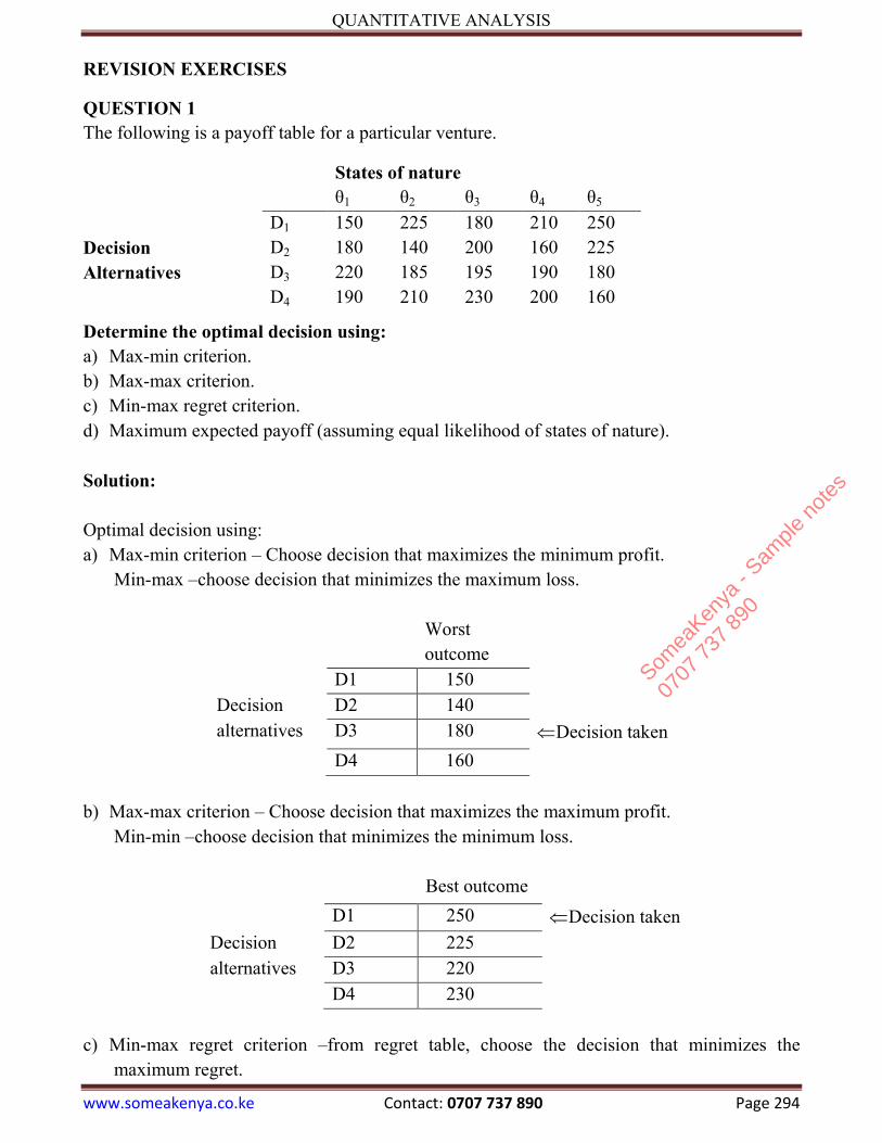
QUANTITATIVE ANALYSIS
www.someakenya.co.ke Contact: 0707 737 890 Page 294
REVISION EXERCISES
QUESTION 1
The following is a payoff table for a particular venture.
Determine the optimal decision using:
a) Max-min criterion.
b) Max-max criterion.
c) Min-max regret criterion.
d) Maximum expected payoff (assuming equal likelihood of states of nature).
Solution:
Optimal decision using:
a) Max-min criterion – Choose decision that maximizes the minimum profit.
Min-max –choose decision that minimizes the maximum loss.
Worst
outcome
D1 150
Decision D2 140
alternatives D3 180 Decision taken
D4 160
b) Max-max criterion – Choose decision that maximizes the maximum profit.
Min-min –choose decision that minimizes the minimum loss.
Best outcome
D1 250 Decision taken
Decision D2 225
alternatives D3 220
D4 230
c) Min-max regret criterion –from regret table, choose the decision that minimizes the
maximum regret.
States of nature
θ1 θ2 θ3 θ4 θ5
D1 150 225 180 210 250
Decision D2 180 140 200 160 225
Alternatives D3 220 185 195 190 180
D4 190 210 230 200 160
Somea
Kenya
- Sam
ple n
otes
0707
737
890

QUANTITATIVE ANALYSIS
www.someakenya.co.ke Contact: 0707 737 890 Page 295
Regret = maximum payoff for a state of nature less the payoff of a given state in a decision
alternative. E.g. regret for: D11 = 220 - 150 = 70
D31 = 210 - 190 = 20
Regret table:
States of Nature
θ1 θ2 θ3 θ4 θ5 Max Either
D1 70 0 50 0 0 70 Decision
Decision D2 40 85 30 50 25 85
alternative D3 0 40 35 20 70 70 Or this
D4 30 15 0 10 90 90
d) Maximum expected payoff –assuming equal likelihood of states of nature, decision that
maximizes the expected payoff determined is taken.
For example:
Expected payoff for D2 = Payoff (D21 + D22 + D23 + D24 + D25)/5
= (180 + 140 + 200 + 160 + 225)/5 = 181
Expected Payoff
D1 203 Decision taken
Decision D2 181
alternative D3 194
D4 198
QUESTION 2
Assume that Table question 1, is a loss table rather than a payoff table. Determine the optimal
decision using:
a) The min-max criterion, b) The min-min criterion, c) The min-max regret criterion, and d) The minimum expected loss criterion (again assuming equal likelihood of states of nature). Solution:
a) Min-max
Worst
outcome
D1 250
Decision D2 225
alternatives D3 220 Decision taken
D4 230
Somea
Kenya
- Sam
ple n
otes
0707
737
890

This is a SAMPLE (Few pages extracted from the complete notes: Page
numbers reflects the original pages on the complete notes).
It’s meant to show you the topics covered in the notes.
Download more at our websites:
www.someakenya.co.ke or
www.someakenya.com
To get the complete notes either in softcopy form or in
Hardcopy (printed & Binded) form, contact us:
Call/text/whatsApp 0707 737 890
Email: [email protected]
Get news and updates about kasneb by liking our page
www.fb.com/studycpa
Or following us on twitter www.twitter.com/someakenya
Pass on first attempt
“Buy quality notes and avoid refers/retakes which costs more money and time”
Sample/preview is NOT FOR SALE
Somea
Kenya
- Sam
ple n
otes
0707
737
890

QUANTITATIVE ANALYSIS
www.someakenya.co.ke Contact: 0707 737 890 Page 301
TOPIC 8
GAME THEORY
Introduction
Game theory is used to determine the optimum strategy in a competitive situation
When two or more competitors are engaged in making decisions, it may involve conflict of
interest. In such a case the outcome depends not only upon an individuals action but also upon
the action of others. Both competing sides face a similar problem. Hence game theory is a
science of conflict
Game theory does not concern itself with finding an optimum strategy but it helps to improve
the decision process.
Game theory has been used in business and industry to develop bidding tactics, pricing
policies, advertising strategies, timing of the introduction of new models in the market e.t.c.
RULES OF GAME THEORY
i) The number of competitors is finite
ii) There is conflict of interests between the participants
iii) Each of these participants has available to him a finite set of available courses of action i.e. choices
iv) The rules governing these choices are specified and known to all players v) While playing each player chooses a course of action from a list of choices available to
him vi) the outcome of the game is affected by choices made by all of the players. The choices
are to be made simultaneously so that no competitor knows his opponents choice until he is already committed to his own
vii) the outcome for all specific choices by all the players is known in advance and numerically defined
viii) When a competitive situation meets all these criteria above we call it a game
NOTE: only in a few real life competitive situation can game theory be applied because all the
rules are difficult to apply at the same time to a given situation.
ILLUSTRATION
Two players X and Y have two alternatives. They show their choices by pressing two types of
buttons in front of them but they cannot see the opponents move. It is assumed that both
players have equal intelligence and both intend to win the game.
This sort of simple game can be illustrated in tabular form as follows:
Somea
Kenya
- Sam
ple n
otes
0707
737
890

QUANTITATIVE ANALYSIS
www.someakenya.co.ke Contact: 0707 737 890 Page 302
Player Y Button R Button t
Player X Button m X wins 2 points X wins 3 points Button n Y wins 2 points X wins 1 point
The game is biased against Y because if player X presses button m he will always win. Hence Y will be forced to press button r to cut down his losses Alternative Illustration
Player Y Button R Button t
Player X Button m X wins 3 points Y wins 4 points Button n Y wins 2 points X wins 1 point
In this case X will not be able to press button m all the time in order to win(or button n).
similarly Y will not be able to press button r or button t all the time in order to win. In such a
situation each player will exercise his choice for part of the time based on the probability
Standard conventions in game theory Consider the following table
Y 3 -4
X -2 1 X plays row I, Y plays columns I, X wins 3 points
X plays row I, Y plays columns II, X looses 4 points
X plays row II, Y plays columns I, X looses 2 points
X plays row II, Y plays columns II, X wins 1 points
3, -4, -2, 1 are the known pay offs to X(X takes precedence over Y)
here the game has been represented in the form of a matrix. When the games are expressed in
this fashion the resulting matrix is commonly known as PAYOFF MATRIX
STRATEGY
It refers to a total pattern of choices employed by any player. Strategy could be pure or a mixed
one
In a pure strategy, player X will play one row all of the time or player Y will also play one of
this columns all the time.
In a mixed strategy, player X will play each of his rows a certain portion of the time and player
Y will play each of his columns a certain portion of the time.
Somea
Kenya
- Sam
ple n
otes
0707
737
890

This is a SAMPLE (Few pages extracted from the complete notes: Page
numbers reflects the original pages on the complete notes).
It’s meant to show you the topics covered in the notes.
Download more at our websites:
www.someakenya.co.ke or
www.someakenya.com
To get the complete notes either in softcopy form or in
Hardcopy (printed & Binded) form, contact us:
Call/text/whatsApp 0707 737 890
Email: [email protected]
Get news and updates about kasneb by liking our page
www.fb.com/studycpa
Or following us on twitter www.twitter.com/someakenya
Pass on first attempt
“Buy quality notes and avoid refers/retakes which costs more money and time”
Sample/preview is NOT FOR SALE
Somea
Kenya
- Sam
ple n
otes
0707
737
890

QUANTITATIVE ANALYSIS
www.someakenya.co.ke Contact: 0707 737 890 Page 310
TOPIC 9
NETWORK PLANNING AND ANALYSIS
BASIC CONCEPTS Network is a system of interrelationship between jobs and tasks for planning and control of resources of a project by identifying critical part of the project. Activity:Task or job of work, which takes time and resource e.g building a bridge. Its represented by an arrow which indicates where the task begins and ends Event (node):This is a point in time and it indicates the start or finish of an activity e.g in building a bridge, rails installed. Its represented by a circle. Dummy activity: An activity that doesn’t consume time or resources, its merely to show logical dependencies between activities so as abide by rules of drawing a network, its represented by dotted arrow Network. This is a combination of activities and events (including dummy activities) Rules for Drawing a Network
a) A network should only have one start point and one finish point (start event and finish event )
b) All activities must have at least one preceding event (tail event)and at least one succeeding event (head event), but an activity may not share the same tail event and head event.
c) An activity can only start after its tail event has been reached d) An event is only complete after all activities leading to it are complete. e) Activities are identified by alphabetical or numeric codes i.e. A,B,C; 1,2,3 or
identification by head or tail events 1-2, 2-4, 3-4,1-4… f) Loops (a series of activities leading back to the same event) and danglers (activities
which do not link to the overall project)are not allowed
Somea
Kenya
- Sam
ple n
otes
0707
737
890

QUANTITATIVE ANALYSIS
www.someakenya.co.ke Contact: 0707 737 890 Page 311
Dangling activity
B
A CR CA
Dummy Events This is an event that does not consume time or resources, its represented by dotted arrow. Dummies are applied when two or more events occur concurrently and they share the same head and tail events e.g. when a car goes to a garage tires are changed and break pads as well, instead of representing this as;
These events are represented as;
Example of a network Activities 1-2 - where 1 is the preceding event where as 2 is the succeeding event of the activity 1-3 2-4 2-5 3-5 4-5 4-6 5-6 6-7
.1.1.1 Loop
A- Tires Changed
B- Break pads Changed
Car Arrives (CA) Car ready (CR)
1
2
3
4
5
6 7
Somea
Kenya
- Sam
ple n
otes
0707
737
890

QUANTITATIVE ANALYSIS
www.someakenya.co.ke Contact: 0707 737 890 Page 312
TIME ANALYSIS
Assessing the time
After drawing the outline of the network time durations of the activities are then inserted.
a) Time estimates. The analysis of the projects time can be achieved by using :
i. Single time estimates for each activity. These estimates would be based on the
judgment of the individual responsible or by technical calculations using data from
similar projects
ii. Multiple time estimates for each activity. the most usual multiple time estimates are
three estimates for each activity , i.e. optimistic (O), Most Likely (ML), and
Pessimistic (P). These three estimates are combined to give an expected time and the
accepted formula is:
Expected time = 6
4MLPO
For example assume that the three estimates for an activity are
Optimistic 11 days Most likely 15 days Pessimistic 18 days
Expected time =
6
1541811
= 14.8 days
b) Use of time estimates. as three time estimates are converted to a single time estimate there
is no fundamental difference between the two methods as regards the basic time analysis
of a network. However, on completion of the basic time analysis, projects with multiple
time estimates can be further analyzed to give an estimate of the probability of
completing the project by a scheduled date.
c) Time units. Time estimates may be given in any unit, i.e. minutes , hours, days depending
on the project. All times estimates within a project must be in the same units otherwise
confusion is bound to occur.
Basic time analysis – critical path
The critical path of a network gives the shortest time in which the whole project can be
completed. It is the chain of activities with the longest duration times. There may be more than
one critical path which may run through a dummy.
Earliest start times (EST) – Forward pass, Once the activities have been timed we can
assess the total project time by calculating the ESTs for each activity. The EST is the earliest
possible time at which a succeeding activity can start.
Assume the following network has been drawn and the activity times estimated in days.
Somea
Kenya
- Sam
ple n
otes
0707
737
890

QUANTITATIVE ANALYSIS
www.someakenya.co.ke Contact: 0707 737 890 Page 313
B
2
A
1
E
1
C
3
F
2
D
4
B
2
A
1
E
1
C
3
F
2
D
4
The ESTs can be inserted as follows.
EST
The method used to insert the ESTs is also known as the forward pass, this is obtained by;
EST = The greater of [EST (tail event) + Activity duration]
a) Start from the start event giving it 0 values,
b) For the rest of the events EST is obtained by summing the EST of the tail event and the
activity duration
c) Where two or more routes converge into an activity, calculate individual EST per route
and the select the longest route (time)
d) The EST of the finish event is the shortest time the whole project can be completed.
Latest Start Times (LST) – Backward pass. this is the latest possible time with which a
preceding activity can finish without increasing the project duration. After this operation the
critical path will be clearly defined.
From our example this is done as follows;
2
0 1
3
4 5
2
3
0
0
1
1
3
4
4
7
5
9
Somea
Kenya
- Sam
ple n
otes
0707
737
890

This is a SAMPLE (Few pages extracted from the complete notes: Page
numbers reflects the original pages on the complete notes).
It’s meant to show you the topics covered in the notes.
Download more at our websites:
www.someakenya.co.ke or
www.someakenya.com
To get the complete notes either in softcopy form or in
Hardcopy (printed & Binded) form, contact us:
Call/text/whatsApp 0707 737 890
Email: [email protected]
Get news and updates about kasneb by liking our page
www.fb.com/studycpa
Or following us on twitter www.twitter.com/someakenya
Pass on first attempt
“Buy quality notes and avoid refers/retakes which costs more money and time”
Sample/preview is NOT FOR SALE
Somea
Kenya
- Sam
ple n
otes
0707
737
890

QUANTITATIVE ANALYSIS
www.someakenya.co.ke Contact: 0707 737 890 Page 325
REVISION EXERCISES
QUESTION 1
a) For the product development project in question 1 consider the detailed time estimates
given in the following table. Note that time estimates in the preceding exercise are
equivalent to modal time estimates in this exercise.
Time Estimates (weeks)
Activity Optimistic Most likely Pessimistic
A
B
C
D
E
F
G
H
1
1
4
1
4
1
1
6
3
1
5
1
6
1
2
8
4
2
9
1
12
2
3
10
Re-label your network in the question 1 to include expected duration ijd (in place of
activity duration dij and variances σij.
Use equations below
6
bm4ad
ijijij
ij
and σij
2
2
6
ijij ab
ijijij ab6 or
b) Compare slacks to those in question 1.
c) Has the critical path changed?
d) Determine the following probabilities:
i) That the project will be completed in 22 weeks or less.
ii) That the project will be completed by its earliest expected completion date.
iii) That the project takes more than 30 weeks to complete.
Solution:
a) Calculation of estimated duration dij and standard deviation of duration ij from the data of
time estimates for the various activities is as follows:
dij =
6
b4ma ijijij and ij
2=2
ij-ij
6
ab
Where: aij- optimistic time
bij- pessimistic time
mij- most likely time
where: aij - optimistic time
bij - pessimistic time
Somea
Kenya
- Sam
ple n
otes
0707
737
890

QUANTITATIVE ANALYSIS
www.someakenya.co.ke Contact: 0707 737 890 Page 326
Activity aij mij bij dij Slack Comment
A 1 3 4 2.8 0.25 8.4 Not critical
B 1 1 2 1.2 0.03 12.3 Not critical
C 4 5 9 5.5 0.69 0 Critical
D 1 1 1 1.0 0.00 9.7 Not critical
E 4 6 12 6.7 1.78 0 Critical
F 1 1 2 1.2 0.03 0 Critical
G 1 2 3 2.0 0.11 0 Critical
H 6 8 10 8.0 0.44 0 Critical
2ij
b) The slacks in this situation are all more than in the situation where optimistic/pessimistic
times are not included.
c) The critical path remained the same being C-E-F-G-H.
d)
i) The variance for the whole project is as follows
2=A2+B
2+C2+D
2+E2+F
2+G2+H
2
2=0.25+0.03+0.69+0+1.78+0.03+0.11+0.44
2=3.6
The expected time of completion is T=23.5 weeks. The probability of completion of
project within t=22 weeks is as follows:
P(t T )=P
σ
Ttz
=P
3.3
5.3222z
A
C
D
B
E
F
G H
5.5
6.7
1.3
1.2
2.8 1
2 8
0
0
2.8
11.2
13.5
13.5
15.5
11.2
23.5
23.5
12.2
12.2
5.5
5.5
0.6
9
1.7
8
0.0
3
0.1
1
0.4
4 0.0
3
0 0.2
5
Somea
Kenya
- Sam
ple n
otes
0707
737
890

This is a SAMPLE (Few pages extracted from the complete notes: Page
numbers reflects the original pages on the complete notes).
It’s meant to show you the topics covered in the notes.
Download more at our websites:
www.someakenya.co.ke or
www.someakenya.com
To get the complete notes either in softcopy form or in
Hardcopy (printed & Binded) form, contact us:
Call/text/whatsApp 0707 737 890
Email: [email protected]
Get news and updates about kasneb by liking our page
www.fb.com/studycpa
Or following us on twitter www.twitter.com/someakenya
Pass on first attempt
“Buy quality notes and avoid refers/retakes which costs more money and time”
Sample/preview is NOT FOR SALE
Somea
Kenya
- Sam
ple n
otes
0707
737
890

QUANTITATIVE ANALYSIS
www.someakenya.co.ke Contact: 0707 737 890 Page 330
TOPIC 10
QUEUING THEORY
INTRODUCTION
Queuing Theory is the study of waiting line which consists of one or more customers waiting
to be served. In queuing theory we analyze the following costs:
i) Waiting costs: These are the costs incurred by the customers waiting on the line. These
costs decrease as the service level increases.
ii) Service cost: These are the costs incurred when the customer is being attended at the
service facility.
The service costs increase as the service level increases. Therefore the total cost in queuing is
the sum of the service costs and the waiting cost.
The main problem in queuing is to determine the optimal service level which minimizes the
total cost.
Generally, the various costs in queuing can be summarized graphically as:
Queuing theory has the following components:
1. Arrivals or calling population
2. Waiting line
3. The service channel or facility
Service cost
TC
Waiting cost
Service Level S
Cos
t
��� �
��
Somea
Kenya
- Sam
ple n
otes
0707
737
890

QUANTITATIVE ANALYSIS
www.someakenya.co.ke Contact: 0707 737 890 Page 331
OPERATING CHARACTERISTICS OF QUEUING SYSTEMS
Analysis of a queuing system involves a study in its different operating characteristics. Some
of them are
1. Queue length (Lq)- The average number of customer in the queue waiting to get service .
This excludeds the customer(s) being served
2. System length (Ls) - the average number of customers in the system including those waiting
as well as those being served.
3. Waiting time in the queue (Wq) - the average time for which a customer has to wait in the
queue to get service.
4. Total time in the system (WS) - the average total time spent by a customer in the system
from the moment he arrives till he leaves the system. It is taken to be the waiting time plus
the service time.
5. Utilization factor (p) - It is the proportion of time a server actually spends with the
customers. It is also called traffic Intensity.
WAITING TIME AND IDLE TIME COSTS
In order to solve a queuing problem, service facility must be manipulated so that an optimum
balance is obtained between the cost of waiting time and the cost of idle time.
The cost of waiting customers generally includes either the indirect cost of lost business
(because people go somewhere else, but less than they had intended to, or do not come again
in future) or direct cost of idle equipment and persons; for example, cost of truck drivers and
equipment waiting to be unloaded or cost of operating an airplane or ship waiting to land or
dock.
The cost of lost business is not easy to assess, e.g., vehicle drivers wanting petrol will avoid
pumps having long queues. To determine how much business is lost, some type of
experimentation and data collection is required.
The cost of idle service facilities is the payment to be made to the servers engaged at the
facilities for the period for which they remain idle.
The waiting time cost is added to the cost of providing service to establish a total expected
cost.
The total expected cost is minimum at a service level denoted by point S. Thus the objective of
the technique is really to determine that particular level of service which minimizes the total
cost of providing service and waiting for that service.
Somea
Kenya
- Sam
ple n
otes
0707
737
890

QUANTITATIVE ANALYSIS
www.someakenya.co.ke Contact: 0707 737 890 Page 332
Therefore the issue of concern to the management is to determine the optimal service rate, S,
that will minimize the total cost associated with the waiting line
Let Cw = expected waiting cost / unit / unit time
Ls = expected (average) number of units in the system
Cf = cost of servicing one unit
Therefore expected waiting cost per time (period) = Cw x Ls = Cw�
���
And expected service cost per unit time (period) = Cf.�
Therefore total cost, C = Cw�
��� + �Cf
This will be minimum if:- �
�� (C) = 0
��
�� = Cw� (� − �)- 1+1 + Cf� = -Cw
�
(���)� + Cf = 0 make � the subject of formula
(� − �)�Cf = Cw�
(���)� x (� − �)�
(� − �)� ��
�� =
����
��
�(� − �)� = �����
��
� − � = �����
��
� = ���
��� + �
Waiting time cost
Increase services
Cost of providing services Total expected cost T
ota
l ex
pec
ted
co
st o
f op
erat
ing
fa
cult
y
0 S
Somea
Kenya
- Sam
ple n
otes
0707
737
890

This is a SAMPLE (Few pages extracted from the complete notes: Page
numbers reflects the original pages on the complete notes).
It’s meant to show you the topics covered in the notes.
Download more at our websites:
www.someakenya.co.ke or
www.someakenya.com
To get the complete notes either in softcopy form or in
Hardcopy (printed & Binded) form, contact us:
Call/text/whatsApp 0707 737 890
Email: [email protected]
Get news and updates about kasneb by liking our page
www.fb.com/studycpa
Or following us on twitter www.twitter.com/someakenya
Pass on first attempt
“Buy quality notes and avoid refers/retakes which costs more money and time”
Sample/preview is NOT FOR SALE
Somea
Kenya
- Sam
ple n
otes
0707
737
890

QUANTITATIVE ANALYSIS
www.someakenya.co.ke Contact: 0707 737 890 Page 340
REVISION EXERCISES
QUESTION 1
In a three channel system, the rate of service at each channel is 5 customers per hour and
customers arrive at the rate of 12 per hour. What is the probability that there are no customers
in the system at a given point in time?
Solution:
C= 3, = 12, = 5, = 12/3 x 5 = 0.8 P0 = 3! (1 – 0.8) (0.8 x 3)3 + 3! (1 – 0.8 (x) Where x = c-11 (c)n n!
= 3 x 2 x 1 (0.2) (2.4)3 + 3 x 2 x 1) (0.2) (x) x is the sum of 3 figures giving 1 ((c)n where n = 0; 1 (0.8 x 3)o = 1.0 0! n = 1 ; 1 (0.83 x 3) 1= 2.4 1! n = 2 ; 1 (0.8 x 3) 2 = ½ (2.4) 2 = 2.88 2! X 6.28 Po = 1.2 = 0.056 13.824 + 1.2 (6.28)
C= 3, = 12, = 5, = 12/3 x 5 = 0.8 P0 = 3! (1 – 0.8) (0.8 x 3)3 + 3! (1 – 0.8 (x) Where x = c-11 (c)n n! = 3 x 2 x 1 (0.2) (2.4)3 + 3 x 2 x 1) (0.2) (x)
Somea
Kenya
- Sam
ple n
otes
0707
737
890

QUANTITATIVE ANALYSIS
www.someakenya.co.ke Contact: 0707 737 890 Page 341
x is the sum of 3 figures giving 1 ((c)n where n = 0; 1 (0.8 x 3)o = 1.0 0! n = 1 ; 1 (0.83 x 3) 1= 2.4 1! n = 2 ; 1 (0.8 x 3) 2 = ½ (2.4) 2 = 2.88 2! X 6.28 Po = 1.2 = 0.056 13.824 + 1.2 (6.28)
QUESTION 2
A team of 15 men is employed to unload lorries at a terminal. The team works a 6 hour day
during which 36 lorries arrive (i.e. 6 per hour) and it takes 7 ½ minutes to unload one lorry
with the team acting as a single unit. Lorries are Served on a FIFO basis.
It has been estimated that the cost of keeping lorries waiting is Sh 6 per hour. Members of the
team are each paid Sh 2.50 per hour. It is also estimated that if the size of the team increased
to 20 men, the average service time would fall to 5 minutes.
Required;-
Calculate the cost of the present system and the cost of the proposed system, and determine
whether an increase in the size of the team would be justified on grounds of cost.
Solution:
The cost of service with
15 man team = 15 x 2.50 x 6 = sh. 225 per day
20 man team = 20 x 2.50 x 6 = sh. 300 per day
The daily cost of lorry waiting time, at sh.6 per hour may be calculated in either of 2 ways.
by calculating the average number of lorries in the system and multiplying this number by (sh
6 per hour x 6 hours per day) Sh. 36 per day or by calculating the average waiting time in the
system, and multiplying this time by sh.6 per hour and by the number of lorries in a 6 hour day
i.e. 36.
Average number of customers in the system = λ or P µ - λ 1 – P 15 man team 20 man team λ =6 µ = 60/7.5=8 P =0.75 λ =6 µ = 60/5=12 P =0.5
Somea
Kenya
- Sam
ple n
otes
0707
737
890

This is a SAMPLE (Few pages extracted from the complete notes: Page
numbers reflects the original pages on the complete notes).
It’s meant to show you the topics covered in the notes.
Download more at our websites:
www.someakenya.co.ke or
www.someakenya.com
To get the complete notes either in softcopy form or in
Hardcopy (printed & Binded) form, contact us:
Call/text/whatsApp 0707 737 890
Email: [email protected]
Get news and updates about kasneb by liking our page
www.fb.com/studycpa
Or following us on twitter www.twitter.com/someakenya
Pass on first attempt
“Buy quality notes and avoid refers/retakes which costs more money and time”
Sample/preview is NOT FOR SALE
Somea
Kenya
- Sam
ple n
otes
0707
737
890

QUANTITATIVE ANALYSIS
www.someakenya.co.ke Contact: 0707 737 890 Page 345
TOPIC 11
SIMULATION
INTRODUCTION
Simulation can be defined as a technique that imitates the operation as it evolves over time. It
is basically a technique of conducting experiments on a model of a system. Simulation model
usually takes the form of a set of assumptions about the operation of the system, expressed as
mathematical or logical relations between the objects of interest in the system.
In order to study a system once it is defined, two alternatives are available:-
i) To study the actual system itself and the other
ii) To construct the model of the system and study the model
Generally the study of the actual system has the disadvantages of being time consuming,
expensive and / or outright impossible (e.g. in a saw mill operation, it would be extremely time
consuming and costly to try every possibility of cutting logs to maximize profit Likewise it
would be impossible to study a proposed system without constructing some form of model.
Consequently models most existing or proposed systems are constructed and the models are
analysed how the actual system will react to change. However, many realistic systems can't be
modeled for solution by the standard operation research methods. Therefore some form of
simulation must be used to provide the solution. Simulation is a general method which can-be
used to solve problems in many areas of management such as
i) Inventory management
ii) Queuing problems
iii) Capital budgeting
iv) Project management
v) Profit planning (CVP analysis etc.)
DEFINITION OF TERMS IN SIMULATION
a) A System - a system can be defined as a collection of entities that act & interact
towards the accomplishment of some logical end. .
b) State of a system- This is the collection of the variables necessary' to describe the status
of the system at any given time. Systems are usually classified as either discrete or
continuous.
c) A discrete system is one which the state variable change only as discrete or countable
points in time
d) A continuous system- is one in which the state variables change continuously over time
Somea
Kenya
- Sam
ple n
otes
0707
737
890

QUANTITATIVE ANALYSIS
www.someakenya.co.ke Contact: 0707 737 890 Page 346
e) Dynamic simulation•-Representation a system as it evolves-overtime.
f) Static simulation model- Representation of a system at a particular point in time
g) Model –a model is a representation of the system and it usually takes the form of a set
of assumption about the operation of the system
There are several types of simulation model namely:
1. Static simulation model
2. Dynamic simulation models
3. Deterministic simulation-models
4. Stochastic simulation models
5. Discrete simulation models
6. Continuous simulation models
Static simulation model
This is a representation of a system at a particular point in time.
Dynamic simulation model
This is a representation of a system as it evolves over time.
Deterministic simulation model
This is a model that contains No random variables.
Stochastic simulation model
This model contains one or more random variables.
WHEN SIMULATION IS USED
i) When the assumptions made are unrealistic or unattainable.
ii) When the system takes too long to observe e.g. demographic / population issues(time
compression advantage)
iii) When, the cost and the danger of experimenting with the real world situations is very
high.
iv) Where there are difficulties in making observations e.g. space research and practice.
Molecular research.
Variables in a simulation model
A business model usually consists of linked series of equations and formulae arranged so that
they 'behave' in a similar manner to the real system being investigated. The formulae and
equations use a number of factors or variables which can be classified into 4 groups.
(a) Input or exogenous variables
(b) Parameters
(c) Status variables
(d) Output or endogenous variables
Somea
Kenya
- Sam
ple n
otes
0707
737
890

QUANTITATIVE ANALYSIS
www.someakenya.co.ke Contact: 0707 737 890 Page 347
These are described below.
a) Input variables
These variables are of two types - controlled and non-controlled.
Controlled variables: These are the variables that can be controlled by management. Changing
the input values of the controlled values and noting the change in the output results is the prime
activity of simulation. For example, typical controlled variables in an inventory simulation
might be the re-order level and re-order quantity. These could be altered and the effect on the
system outputs noted.
Non-controlled variables: These are Input variables which are not under management control.
Typically these are probabilistic or stochastic variables i.e., they vary but in some
uncontrollable probabilistic fashion.
For example, in a production simulation the number of breakdowns would be deemed to vary
in accordance with a probability distribution derived from records of past breakdown
frequencies.' In an inventory simulation demand and lead time would also be generally
classified as non- controlled, probabilistic variables
b) Parameters
These are also input variables which, for a given simulation have a constant value. Parameters
are factors which help to specify the relationships between other types of variables. For
example in a production simulation a parameter (or constant) might be the time taken for
routine maintenance, in an inventory simulation a parameter might be the cost of a stock-out.
c) Status variables
In some types of simulation the behavior of the system (rates, usages, speeds, demand and so
on) varies not only according to individual characteristics but also according to the general
state of the system at various times or seasons. As an example; in a simulation of supermarket
demand and checkout queuing, demand will be probabilistic and variable on any given day but
the general level of demand will be greatly influenced by the day of the week and the season of
the year. Status variables would be required to specify the day(s) and season(s) to be used in a
simulation.
Note: On occasions status variables and parameters would both be termed just parameters
although strictly speaking there is a difference between the two concepts.
d) Output variables
These are the results of the simulation. They arise from the calculations and tests performed in
the model the input values of the controlled values. The values derived for me probabilistic
elements and the specified parameters and status values. The output variables must be carefully
chosen to reflect the factors which are critical to the really system being simulated and they
related to the objectives of the really system. For example, output variables for an inventory
simulation would typically include:
Somea
Kenya
- Sam
ple n
otes
0707
737
890

This is a SAMPLE (Few pages extracted from the complete notes: Page
numbers reflects the original pages on the complete notes).
It’s meant to show you the topics covered in the notes.
Download more at our websites:
www.someakenya.co.ke or
www.someakenya.com
To get the complete notes either in softcopy form or in
Hardcopy (printed & Binded) form, contact us:
Call/text/whatsApp 0707 737 890
Email: [email protected]
Get news and updates about kasneb by liking our page
www.fb.com/studycpa
Or following us on twitter www.twitter.com/someakenya
Pass on first attempt
“Buy quality notes and avoid refers/retakes which costs more money and time”
Sample/preview is NOT FOR SALE
Somea
Kenya
- Sam
ple n
otes
0707
737
890

QUANTITATIVE ANALYSIS
www.someakenya.co.ke Contact: 0707 737 890 Page 356
REVISION EXERCISES
QUESTION 1
ABC Ltd. recently acquired a threshing machine with a useful life of 15 years. Over the useful
life, the machine is likely to have periodic failures and breakdowns. Past data for similar
machines indicate a probability distribution of failures as follows:
Number of failures 0 1 2 3
Probability 0.80 0.15 0.04 0.01
Required:
(i) Using the random numbers provided below, simulate the number of failures that will
occur over the useful life of the machine.
Random numbers: 70,88,37,12,45,99,54,71,64,93,67,80,55,34,22
(ii) Determine the average annual failure rate.
Solution:
No of failures Probability Cumulative probability RN - Ranges 0 1 2 3
0.80 0.15 0.04 0.01
0.80 0.95 0.99 1.00
00 – 79 80 – 94 95 – 98 99 >
Simulation Worksheet
Years Random numbers No of failures 1 2 3 4 5 6 7 8 9 10 11 12 13 14 15
70 88 37 12 45 99 54 71 64 93 67 80 55 34 22
0 1 0 0 0 3 0 0 0 1 0 1 0 0 0 6
Average annual failure rate = 6 = 0.4 15
Somea
Kenya
- Sam
ple n
otes
0707
737
890

QUANTITATIVE ANALYSIS
www.someakenya.co.ke Contact: 0707 737 890 Page 357
QUESTION 2
(a) Manukato Ltd. produces a designer perfume called “Hint of Elegance.” Production of
the perfume involves the use of two ingredients, X1 and X2 represented by the
production function given below:
Y = 21XX
Where Y = Number of bottles of designer perfume produced.
X1 = Units of ingredient 1.
X2 = Units of ingredient 2.
Currently, the company is operating at a level where the daily usage of X1 and X2 is set at 250
units and 360 units respectively.
The price of the designer perfume and the cost of ingredients X1 and X2 are random variables.
The data below relate to the three random variables.
Selling price of Y (per bottle)
Probabilities
Shs. 4,000 0.15 4,500 0.35 5,000 0.20 5,500 0.30
Cost of ingredient X1 Probabilities
Shs. 1,000 0.10 1,500 0.05 2,000 0.35 2,500 0.50
Cost of ingredient X2 Probabilities
Shs. 1,500 0.20 2,000 0.25 2,500 0.15 3,000 0.40
Required:
(i)Calculate the daily expected profit of the company.
(ii) Simulate the company’s profit for 10 days using the following random numbers:
58, 71, 96, 30, 24, 18, 46, 23, 34, 27, 85, 13, 99, 24, 44, 49,
Somea
Kenya
- Sam
ple n
otes
0707
737
890

This is a SAMPLE (Few pages extracted from the complete notes: Page
numbers reflects the original pages on the complete notes).
It’s meant to show you the topics covered in the notes.
Download more at our websites:
www.someakenya.co.ke or
www.someakenya.com
To get the complete notes either in softcopy form or in
Hardcopy (printed & Binded) form, contact us:
Call/text/whatsApp 0707 737 890
Email: [email protected]
Get news and updates about kasneb by liking our page
www.fb.com/studycpa
Or following us on twitter www.twitter.com/someakenya
Pass on first attempt
“Buy quality notes and avoid refers/retakes which costs more money and time”
Sample/preview is NOT FOR SALE
Somea
Kenya
- Sam
ple n
otes
0707
737
890