quantifying uncertainty & bayesian networks -...
TRANSCRIPT

Quantifying uncertainty & Bayesian networksCE417: Introduction to Artificial Intelligence
Sharif University of Technology
Spring 2015
“Artificial Intelligence: A Modern Approach”, 3rd Edition, Chapter 13, 14 (14.1,14.2,14.4)
Soleymani
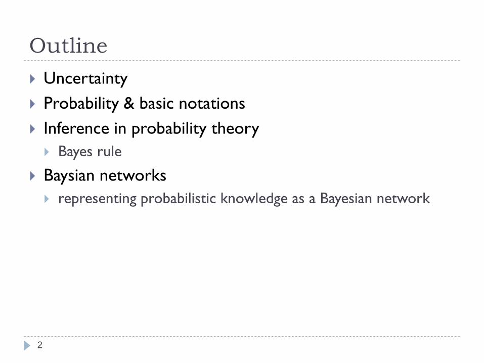
Outline
Uncertainty
Probability & basic notations
Inference in probability theory
Bayes rule
Baysian networks
representing probabilistic knowledge as a Bayesian network
2

Automated taxi example
3
At :“leave for airport t minutes before flight”
“Will At get us to the airport on time?”
“A90 will get us there on time if the car does not break
down or run out of gas and there's no accident on the
bridge and I don’t get into an accident and …”
Qualification problem
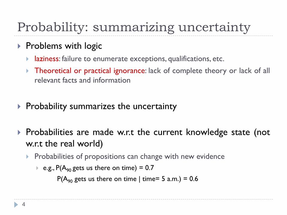
Probability: summarizing uncertainty
Problems with logic
laziness: failure to enumerate exceptions, qualifications, etc.
Theoretical or practical ignorance: lack of complete theory or lack of all
relevant facts and information
Probability summarizes the uncertainty
Probabilities are made w.r.t the current knowledge state (not
w.r.t the real world)
Probabilities of propositions can change with new evidence
e.g., P(A90 gets us there on time) = 0.7
P(A90 gets us there on time | time= 5 a.m.) = 0.6
4

Automated taxi example: rational decision
5
A90 can be a rational decision depending on performance
measure
Performance measure: getting to the airport in time, avoiding a long wait
in the airport, avoiding speeding tickets along the way,…
Maximizing expected utility
Decision theory = probability theory + utility theory
Utility theory: assigning a degree of usefulness for each state and preferring
states with higher utility

Basic probability notations (sets)
6
Sample space (Ω): set of all possible worlds
Probability model
0 ≤ 𝑃(𝜔) ≤ 1 (∀𝜔 ∈ Ω) 𝜔 is an atomic event
𝑃 Ω = 1
𝑃(𝐴) = 𝜔∈𝐴𝑃(𝜔) (∀𝐴 ⊆ Ω) 𝐴 is a set of possible worlds

Basic probability notations (propositions)
7
𝑆: set of all propositional sentences
Probability model
0 ≤ 𝑃(𝑎) ≤ 1 (∀𝑎 ∈ 𝑆)
If 𝑇 is a tautology 𝑃 𝑇 = 1
𝑃(𝜙) = 𝜔∈Ω: 𝜔⊨𝜙𝑃(𝜔) (∀𝜙 ∈ 𝑆)

Basic probability notations (propositions)
8
Each proposition corresponds to a set of possible worlds
A possible world is defined as an assignment of values to all
random variables under consideration.
Elementary proposition
e.g.,𝐷𝑖𝑐𝑒1 = 4
Complex propositions
e.g.,𝐷𝑖𝑐𝑒1 = 4 ∨ 𝐷𝑖𝑐𝑒2 = 6

Random variables
Domain of random variables:Boolean,discrete or continuous
Boolean
e.g.,The domain of 𝐶𝑎𝑣𝑖𝑡𝑦: {𝑡𝑟𝑢𝑒, 𝑓𝑎𝑙𝑠𝑒}
𝐶𝑎𝑣𝑖𝑡𝑦 = 𝑡𝑟𝑢𝑒 is abbreviated as 𝑐𝑎𝑣𝑖𝑡𝑦
Discrete
e.g.,The domain of𝑊𝑒𝑎𝑡ℎ𝑒𝑟 is 𝑠𝑢𝑛𝑛𝑦, 𝑟𝑎𝑖𝑛𝑦, 𝑐𝑙𝑜𝑢𝑑𝑦, 𝑠𝑛𝑜𝑤
Continuous
Probability distribution: the function describing probabilities of
possible values of a random variable
𝑃(𝑊𝑒𝑎𝑡ℎ𝑒𝑟 = 𝑠𝑢𝑛𝑛𝑦) = 0.6, 𝑃 𝑊𝑒𝑎𝑡ℎ𝑒𝑟 = 𝑟𝑎𝑖𝑛 = 0.1, …
9

Probabilistic inference
10
Joint probability distribution
specifies probability of every atomic event
Prior and posterior probabilities
belief in the absence or presence of evidences
Bayes’ rule
used when we don’t have 𝑃(𝑎|𝑏) but we have 𝑃(𝑏|𝑎)
Independence

Probabilistic inference
11
If we consider full joint distribution as KB
Every query can be answered by it
Probabilistic inference: Computing posterior distribution
of variables given evidence
An agent needs to make decisions based on the obtained evidence

Joint probability distribution
12
Joint probability distribution
Probability of all combinations of the values for a set of random vars.
Queries can be answered by summing over atomic events
snowcloudyrainysunnyWeather
0.020.0160.020.144Cavity = true
0.080.0640.080.576Cavity = false
𝐏(𝑊𝑒𝑎𝑡ℎ𝑒𝑟, 𝐶𝑎𝑣𝑖𝑡𝑦) : joint probability as a 4 × 2 matrix of values

Prior and posterior probabilities
Prior or unconditional probabilities of propositions: belief in
the absence of any other evidence
e.g.,𝑃 𝑐𝑎𝑣𝑖𝑡𝑦 = 0.2
𝑃(𝑊𝑒𝑎𝑡ℎ𝑒𝑟 = 𝑠𝑢𝑛𝑛𝑦) = 0.72
Posterior or conditional probabilities: belief in the presence of
evidences
e.g.,𝑃(𝑐𝑎𝑣𝑖𝑡𝑦 | 𝑡𝑜𝑜𝑡ℎ𝑎𝑐ℎ𝑒)
𝑃(𝑎|𝑏) = 𝑃(𝑎 ∧ 𝑏) 𝑃(𝑏) if 𝑃(𝑏) > 0
13

Sum rule and product rule
Product rule (obtained from the formulation of the conditional
probability):
𝑃(𝑎, 𝑏) = 𝑃(𝑎|𝑏) 𝑃(𝑏) = 𝑃(𝑏|𝑎) 𝑃(𝑎)
Sume rule:
𝑃(𝑎) =
𝑏
𝑃(𝑎, 𝑏)
14

Inference: example
Joint probability distribution:
Conditional probabilities:
𝑃(¬𝑐𝑎𝑣𝑖𝑡𝑦 | 𝑡𝑜𝑜𝑡ℎ𝑎𝑐ℎ𝑒)
=𝑃(¬𝑐𝑎𝑣𝑖𝑡𝑦 ∧ 𝑡𝑜𝑜𝑡ℎ𝑎𝑐ℎ𝑒)
𝑃(𝑡𝑜𝑜𝑡ℎ𝑎𝑐ℎ𝑒)
= 𝑐𝑎𝑡𝑐ℎ=𝑇,𝐹 𝑃(¬𝑐𝑎𝑣𝑖𝑡𝑦, 𝑡𝑜𝑜𝑡ℎ𝑎𝑐ℎ𝑒, 𝑐𝑎𝑡𝑐ℎ)
𝑐𝑎𝑡𝑐ℎ=𝑇,𝐹 𝑐𝑎𝑣𝑖𝑡𝑦=𝑇,𝐹 𝑃(𝑐𝑎𝑣𝑖𝑡𝑦, 𝑡𝑜𝑜𝑡ℎ𝑎𝑐ℎ𝑒, 𝑐𝑎𝑡𝑐ℎ)
=0.016 + 0.064
0.108 + 0.012 + 0.016 + 0.064= 0.4
15
¬𝑡𝑜𝑜𝑡𝑎𝑐ℎ𝑒𝑡𝑜𝑜𝑡𝑎𝑐ℎ𝑒
¬𝑐𝑎𝑡𝑐ℎ𝑐𝑎𝑡𝑐ℎ¬𝑐𝑎𝑡𝑐ℎ𝑐𝑎𝑡𝑐ℎ
0.0080.0720.0120.108𝑐𝑎𝑣𝑖𝑡𝑦
0.5760.1440.0640.016¬𝑐𝑎𝑣𝑖𝑡𝑦
𝐏 𝒚|𝐞 = 𝒛𝐏 𝒛, 𝐞, 𝐲
𝒛 𝒚𝐏 𝒛, 𝐞, 𝐲

Bayes' rule
Bayes' rule:𝑃(𝑎|𝑏) = 𝑃(𝑏|𝑎) 𝑃(𝑎) / 𝑃(𝑏)
𝑃 𝑎𝑏 = 𝑃 𝑎 𝑏 𝑃 𝑏 = 𝑃 𝑏 𝑎 𝑃 𝑎
In many problems, it may be difficult to compute 𝑃(𝑎|𝑏)directly, yet we might have information about 𝑃(𝑏|𝑎).
Computing diagnostic probability from causal probability:
𝑃(𝐶𝑎𝑢𝑠𝑒|𝐸𝑓𝑓𝑒𝑐𝑡) = 𝑃(𝐸𝑓𝑓𝑒𝑐𝑡|𝐶𝑎𝑢𝑠𝑒) 𝑃(𝐶𝑎𝑢𝑠𝑒) / 𝑃(𝐸𝑓𝑓𝑒𝑐𝑡)
16
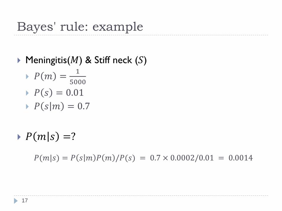
Bayes' rule: example
17
Meningitis(𝑀) & Stiff neck (𝑆)
𝑃 𝑚 =1
5000
𝑃 𝑠 = 0.01
𝑃 𝑠 𝑚 = 0.7
𝑃 𝑚 𝑠 =?
𝑃(𝑚|𝑠) = 𝑃 𝑠 𝑚 𝑃 𝑚 /𝑃(𝑠) = 0.7 × 0.0002/0.01 = 0.0014

Independence
Propositions 𝑎 and 𝑏 are independent iff
𝑃(𝑎|𝑏) = 𝑃(𝑎)
𝑃 𝑏 𝑎 = 𝑃 𝑏
𝑃(𝑎, 𝑏) = 𝑃(𝑎) 𝑃(𝑏)
𝑛 independent biased coins
The number of required independent probabilities
is reduced from 2𝑛 − 1 to 𝑛
18

Independence
𝑃 𝑡𝑜𝑜𝑡ℎ𝑎𝑐ℎ𝑒, 𝑐𝑎𝑡𝑐ℎ, 𝑐𝑎𝑣𝑖𝑡𝑦, 𝑐𝑙𝑜𝑢𝑑𝑦
= 𝑃(𝑡𝑜𝑜𝑡ℎ𝑎𝑐ℎ𝑒, 𝑐𝑎𝑡𝑐ℎ, 𝑐𝑎𝑣𝑖𝑡𝑦) 𝑃(𝑐𝑙𝑜𝑢𝑑𝑦)
19
The number of required independent probabilities is reduced from
21 = (23 − 1) × (4 − 1)to 10 = (23−1) + (4 − 1)
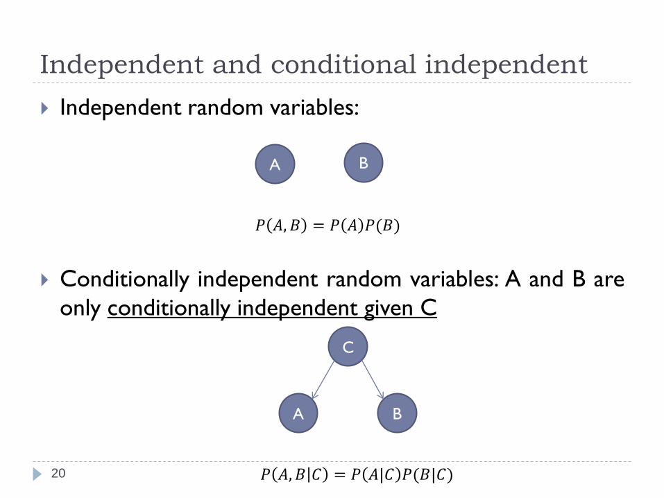
Independent and conditional independent
20
Independent random variables:
Conditionally independent random variables: A and B are
only conditionally independent given C
A B
C
𝑃 𝐴, 𝐵 𝐶 = 𝑃 𝐴|𝐶 𝑃(𝐵|𝐶)
A B
𝑃 𝐴, 𝐵 = 𝑃 𝐴 𝑃(𝐵)

Cavity example
Topology of network encodes conditional independencies
21
𝑊𝑒𝑎𝑡ℎ𝑒𝑟 is independent of the other variables
𝑇𝑜𝑜𝑡ℎ𝑎𝑐ℎ𝑒 and 𝐶𝑎𝑡𝑐ℎ are conditionally
independent given 𝐶𝑎𝑣𝑖𝑡𝑦

Wumpus example
22
𝑏 = ¬𝑏1,1 ∧ 𝑏1,2 ∧ 𝑏2,1
𝑘𝑛𝑜𝑤𝑛 = ¬𝑝1,1 ∧ ¬𝑝1,2 ∧ ¬𝑝2,1
𝑃 𝑃1,3 𝑘𝑛𝑜𝑤𝑛, 𝑏 =?

Wumpus example
23
Possible worlds with 𝑃1,3 = 𝑡𝑟𝑢𝑒 Possible worlds with 𝑃1,3 = 𝑓𝑎𝑙𝑠𝑒
𝑃 𝑃1,3 = 𝑇𝑟𝑢𝑒 𝑘𝑛𝑜𝑤𝑛, 𝑏 ∝ 0.2 × 0.2 × 0.2 + 0.2 × 0.8 + 0.8 × 0.2
𝑃 𝑃1,3 = 𝐹𝑎𝑙𝑠𝑒 𝑘𝑛𝑜𝑤𝑛, 𝑏 ∝ 0.8 × 0.2 × 0.2 + 0.2 × 0.8
⇒ 𝑃 𝑃1,3 = 𝑇𝑟𝑢𝑒 𝑘𝑛𝑜𝑤𝑛, 𝑏 = 0.31

Bayesian networks
Importance of independence and conditional independence
relationships (to simplify representation)
Bayesian network: a graphical model to represent
dependencies among variables
compact specification of full joint distributions
easier for human to understand
24

Bayesian network
25
Bayesian network is a directed acyclic graph
Each node shows a random variable
Each link from 𝑋 to 𝑌 shows a "direct influence“ of 𝑋 on 𝑌 (𝑋 is a
parent of 𝑌)
For each node, a conditional probability distribution 𝐏(𝑋𝑖|𝑃𝑎𝑟𝑒𝑛𝑡𝑠(𝑋𝑖))
shows the effects of parents on the node

Constructing a Bayesian network
26
How to construct a network for a specific problem?
Identify random variables
Determine conditional dependencies
Constructing CPDs
We need prior knowledge of modular relationships and causal
relationships

Burglary example
“A burglar alarm, respond occasionally to minor earthquakes.
Neighbors John and Mary call you when hearing the alarm.
John nearly always calls when hearing the alarm.
Mary often misses the alarm.”
Variables:
𝐵𝑢𝑟𝑔𝑙𝑎𝑟𝑦
𝐸𝑎𝑟𝑡ℎ𝑞𝑢𝑎𝑘𝑒
𝐴𝑙𝑎𝑟𝑚
𝐽𝑜ℎ𝑛𝐶𝑎𝑙𝑙𝑠
𝑀𝑎𝑟𝑦𝐶𝑎𝑙𝑙𝑠
27

Burglary example: DAG + CPTs
28
Conditional Probability Table
(CPT)
𝑃(𝐽 = 𝑓|𝐴)𝑃(𝐽 = 𝑡|𝐴)𝐴
0.10.9𝑡
0.950.05𝑓
CPTs as
quantitative
specification
𝑷(𝑨 = 𝒕|𝑩, 𝑬)
𝑷(𝑱 = 𝒕|𝑨) 𝑷(𝑴 = 𝒕|𝑨)
John nearly always calls when hearing the alarm.
Mary often calls when hearing the alarm.

Burglary example
29
John do not perceive
burglaries directly
John do not perceive
minor earthquakes

Accuracy-complexity tradeoff
30
We may not consider some of variables or links
Importance of getting more accurate probabilities vs. the cost of
specifying the extra information
It may not be worth the additional complexity in the network for the
small gain in accuracy
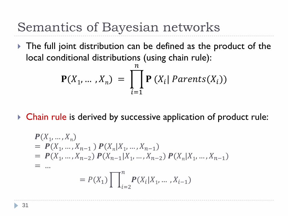
The full joint distribution can be defined as the product of the
local conditional distributions (using chain rule):
𝐏(𝑋1, … , 𝑋𝑛) =
𝑖=1
𝑛
𝐏 (𝑋𝑖| 𝑃𝑎𝑟𝑒𝑛𝑡𝑠(𝑋𝑖))
Chain rule is derived by successive application of product rule:
𝑷(𝑋1, … , 𝑋𝑛)= 𝑷(𝑋1, … , 𝑋𝑛−1 ) 𝑷(𝑋𝑛|𝑋1, … , 𝑋𝑛−1)= 𝑷(𝑋1, … , 𝑋𝑛−2) 𝑷(𝑋𝑛−1|𝑋1, … , 𝑋𝑛−2) 𝑷(𝑋𝑛|𝑋1, … , 𝑋𝑛−1)= …
= 𝑃(𝑋1) 𝑖=2
𝑛
𝑷(𝑋𝑖|𝑋1, … , 𝑋𝑖−1)
Semantics of Bayesian networks
31

Burglary example (joint probability)
32
We can compute joint probabilities from CPTs:
𝑃 𝑗 ∧ 𝑚 ∧ 𝑎 ∧ 𝑏 ∧ 𝑒
= 𝑃 (𝑗 | 𝑎) 𝑃 (𝑚 | 𝑎) 𝑃 𝑎 𝑏 ∧ 𝑒) 𝑃 (𝑏) 𝑃 (𝑒)
= 0.9 × 0.7 × 0.001 × 0.999 × 0.998 = 0.000628

Joint distribution in Bayesian networks
33
Indeed, we simplify chain rule through conditional
independencies assumptions:
𝑃 𝑋𝑖 𝑋1, 𝑋2, … , 𝑋𝑖−1) = 𝑃(𝑋𝑖| 𝑃𝑎𝑟𝑒𝑛𝑡𝑠(𝑋𝑖))
For each node, a CPD 𝑃(𝑋𝑖|𝑃𝑎𝑟𝑒𝑛𝑡𝑠(𝑋𝑖)) shows the
effects of parents on the node.
Conditional independencies:
Each node 𝑋𝑖 is conditionally independent of
𝑋1, 𝑋2, … , 𝑋𝑖−1, given only its immediate parents.

Bayesian network: Example
Naïve Bayes model:
𝐏(𝐶𝑎𝑢𝑠𝑒, 𝐸𝑓𝑓𝑒𝑐𝑡1, … , 𝐸𝑓𝑓𝑒𝑐𝑡𝑛) = 𝐏(𝐶𝑎𝑢𝑠𝑒)
𝑖=1
𝑛
𝐏(𝐸𝑓𝑓𝑒𝑐𝑡𝑖|𝐶𝑎𝑢𝑠𝑒)
Example
34

Compactness
Locally structured
A CPT for a Boolean variable with k Boolean parents requires:
2𝑘 rows for the combinations of parent values
𝑘 = 0 (one row showing prior probabilities of each possible value of
that variable)
If each variable has no more than 𝑘 parents
Baysian network requires 𝑂(𝑛 × 2𝑘) numbers (linear with 𝑛)
Full joint distribution requires 𝑂 2𝑛 numbers
35

Constructing Bayesian networks
I. Nodes:
determine the set of variables and order them as 𝑋1, … , 𝑋𝑛
(More compact network if causes precede effects)
II. Links:
for 𝑖 = 1 to 𝑛
1) select a minimal set of parents for 𝑋𝑖 from 𝑋1, … , 𝑋𝑖−1 such that
𝐏(𝑋𝑖 | 𝑃𝑎𝑟𝑒𝑛𝑡𝑠(𝑋𝑖)) = 𝐏(𝑋𝑖 | 𝑋1, … 𝑋𝑖−1)
2) For each parent insert a link from the parent to 𝑋𝑖
3) CPT creation based on 𝐏(𝑋𝑖 | 𝑋1, … 𝑋𝑖−1)
36

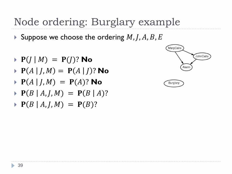
Suppose we choose the ordering 𝑀, 𝐽, 𝐴, 𝐵, 𝐸
𝐏 𝐽 𝑀) = 𝐏(𝐽)?
Node ordering: Burglary example
37

Suppose we choose the ordering 𝑀, 𝐽, 𝐴, 𝐵, 𝐸
𝐏 𝐽 𝑀) = 𝐏(𝐽)? No
𝐏 𝐴 𝐽,𝑀 = 𝐏 𝐴 𝐽 ?
𝐏 𝐴 𝐽,𝑀) = 𝐏(𝐴)?
Node ordering: Burglary example
38
Suppose we choose the ordering 𝑀, 𝐽, 𝐴, 𝐵, 𝐸
𝐏 𝐽 𝑀) = 𝐏(𝐽)? No
𝐏 𝐴 𝐽,𝑀 = 𝐏 𝐴 𝐽 ?No
𝐏 𝐴 𝐽,𝑀) = 𝐏(𝐴)? No
𝐏 𝐵 𝐴, 𝐽,𝑀) = 𝐏 𝐵 𝐴)?
𝐏 𝐵 𝐴, 𝐽,𝑀) = 𝐏(𝐵)?
Node ordering: Burglary example
39
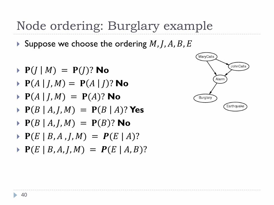
Suppose we choose the ordering 𝑀, 𝐽, 𝐴, 𝐵, 𝐸
𝐏 𝐽 𝑀) = 𝐏(𝐽)? No
𝐏 𝐴 𝐽,𝑀 = 𝐏 𝐴 𝐽 ?No
𝐏 𝐴 𝐽,𝑀) = 𝐏(𝐴)? No
𝐏 𝐵 𝐴, 𝐽,𝑀) = 𝐏 𝐵 𝐴)? Yes
𝐏 𝐵 𝐴, 𝐽,𝑀) = 𝐏 𝐵 ? No
𝐏(𝐸 | 𝐵, 𝐴 , 𝐽,𝑀) = 𝑷(𝐸 | 𝐴)?
𝐏(𝐸 | 𝐵, 𝐴, 𝐽,𝑀) = 𝑷(𝐸 | 𝐴, 𝐵)?
Node ordering: Burglary example
40

Suppose we choose the ordering 𝑀, 𝐽, 𝐴, 𝐵, 𝐸
𝐏 𝐽 𝑀) = 𝐏(𝐽)? No
𝐏 𝐴 𝐽,𝑀 = 𝐏 𝐴 𝐽 ?No
𝐏 𝐴 𝐽,𝑀) = 𝐏(𝐴)? No
𝐏 𝐵 𝐴, 𝐽,𝑀) = 𝐏 𝐵 𝐴)? Yes
𝐏 𝐵 𝐴, 𝐽,𝑀) = 𝐏(𝐵)? No
𝐏(𝐸 | 𝐵, 𝐴 , 𝐽,𝑀) = 𝑷(𝐸 | 𝐴)?No
𝐏(𝐸 | 𝐵, 𝐴, 𝐽,𝑀) = 𝑷(𝐸 | 𝐴, 𝐵)?Yes
Node ordering: Burglary example
41

Causal models
42
Some new links represent relationships that require difficult and unnatural
probability judgments
Deciding conditional independence is hard in non-causal directions

Node ordering: burglary example
The structure of the network and so the number of required probabilities
for different node orderings can be different
43
1 + 2 + 4 + 2 + 4 = 131 + 1 + 4 + 2 + 2 = 10
4
2 2
1 1
1 + 2 + 4 + 8 + 16 = 31
4
4
2
2
1 1
2
4
8
16

Why using Bayesian networks?
44
Compact representation of probability distributions: smaller
number of parameters
Instead of storing full joint distribution requiring large number of
parameters
Incorporation of domain knowledge and causal structures
Algorithm for systematic and efficient inference/learning
Exploiting the graph structure and probabilistic semantics
Take advantage of conditional and marginal independences among
random variables
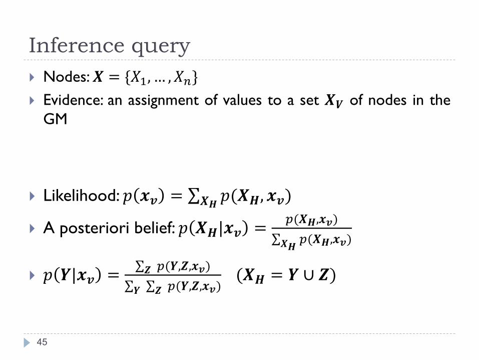
Inference query
45
Nodes:𝑿 = {𝑋1, … , 𝑋𝑛}
Evidence: an assignment of values to a set 𝑿𝑽 of nodes in the
GM
Likelihood: 𝑝 𝒙𝒗 = 𝑿𝑯 𝑝(𝑿𝑯, 𝒙𝒗)
A posteriori belief: 𝑝 𝑿𝑯|𝒙𝒗 =𝑝(𝑿𝑯,𝒙𝒗)
𝑿𝑯𝑝(𝑿𝑯,𝒙𝒗)
𝑝 𝒀|𝒙𝒗 = 𝒁 𝑝(𝒀,𝒁,𝒙𝒗)
𝒀 𝒁 𝑝(𝒀,𝒁,𝒙𝒗)(𝑿𝑯 = 𝒀 ∪ 𝒁)
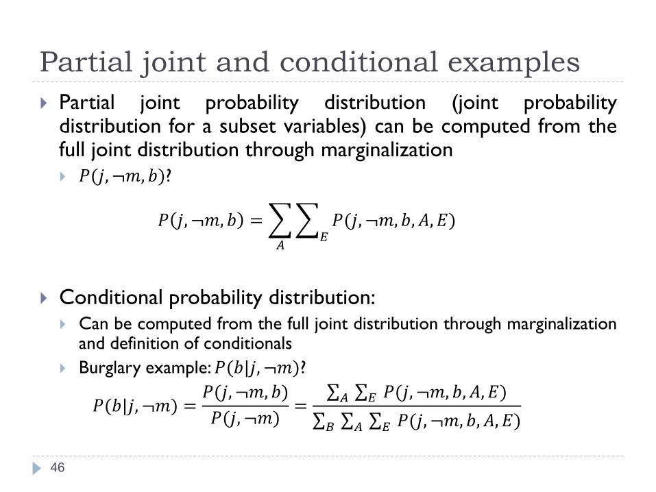
Partial joint and conditional examples
46
Partial joint probability distribution (joint probabilitydistribution for a subset variables) can be computed from thefull joint distribution through marginalization 𝑃(𝑗, ¬𝑚, 𝑏)?
𝑃 𝑗, ¬𝑚, 𝑏 =
𝐴
𝐸𝑃(𝑗, ¬𝑚, 𝑏, 𝐴, 𝐸)
Conditional probability distribution: Can be computed from the full joint distribution through marginalization
and definition of conditionals
Burglary example:𝑃(𝑏|𝑗, ¬𝑚)?
𝑃(𝑏|𝑗, ¬𝑚) =𝑃(𝑗, ¬𝑚, 𝑏)
𝑃(𝑗, ¬𝑚)= 𝐴 𝐸 𝑃(𝑗, ¬𝑚, 𝑏, 𝐴, 𝐸)
𝐵 𝐴 𝐸 𝑃(𝑗, ¬𝑚, 𝑏, 𝐴, 𝐸)
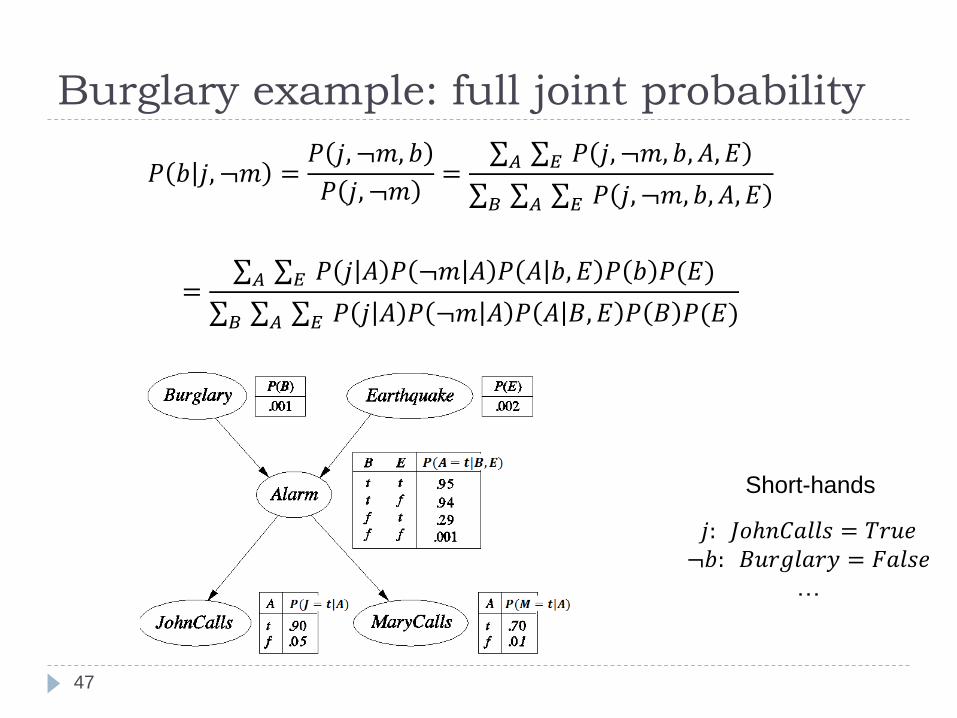
Burglary example: full joint probability
47
𝑃 𝑏 𝑗, ¬𝑚 =𝑃 𝑗, ¬𝑚, 𝑏
𝑃 𝑗, ¬𝑚= 𝐴 𝐸 𝑃 𝑗, ¬𝑚, 𝑏, 𝐴, 𝐸
𝐵 𝐴 𝐸 𝑃 𝑗, ¬𝑚, 𝑏, 𝐴, 𝐸
= 𝐴 𝐸 𝑃 𝑗 𝐴 𝑃 ¬𝑚 𝐴 𝑃 𝐴 𝑏, 𝐸 𝑃 𝑏 𝑃(𝐸)
𝐵 𝐴 𝐸 𝑃 𝑗 𝐴 𝑃 ¬𝑚 𝐴 𝑃 𝐴 𝐵, 𝐸 𝑃 𝐵 𝑃(𝐸)
𝑗: 𝐽𝑜ℎ𝑛𝐶𝑎𝑙𝑙𝑠 = 𝑇𝑟𝑢𝑒¬𝑏: 𝐵𝑢𝑟𝑔𝑙𝑎𝑟𝑦 = 𝐹𝑎𝑙𝑠𝑒
…
Short-hands

Inference in Bayesian networks
48
Computing 𝑝 𝑿𝑯|𝒙𝒗 in an arbitrary GM is NP-hard
Exact inference: enumeration intractable (NP-Hard)
Special cases are tractable
There are many enumeration-based methods

Enumeration
49
𝑃 𝒀 𝒙𝒗 ∝ 𝑃 𝒀, 𝒙𝒗
𝑃 𝒀, 𝒙𝒗 = 𝒁 𝑃(𝒀, 𝒙𝒗, 𝒁) exponential in general
we cannot find a general procedure that works efficiently forarbitrary GMs
Sometimes the structure of the network allows us to infermore efficiently
avoiding exponential cost
Can be improved by re-using calculations
similar to dynamic programming

Distribution of products on sums
50
Exploiting the factorization properties to allow sums and
products to be interchanged
𝑎 × 𝑏 + 𝑎 × 𝑐 needs three operations while 𝑎 × (𝑏 + 𝑐)requires two
Variable elimination: example
51
𝑃 𝑏, 𝑗 = 𝐴
𝐸
𝑀
𝑃 𝑏 𝑃 𝐸 𝑃 𝐴 𝑏, 𝐸 𝑃 𝑗 𝐴 𝑃 𝑀 𝐴
= 𝑃 𝑏
𝐸
𝑃 𝐸
𝐴
𝑃 𝐴 𝑏, 𝐸 𝑃 𝑗 𝐴 𝑀𝑃 𝑀 𝐴
𝑃 𝑏|𝑗 ∝ 𝑃(𝑏, 𝑗)Intermediate results are
probability distributions

Variable elimination: example
52
𝑃 𝐵, 𝑗 = 𝐴
𝐸
𝑀
𝑃 𝐵 𝑃 𝐸 𝑃 𝐴 𝐵, 𝐸 𝑃 𝑗 𝐴 𝑃 𝑀 𝐴
= 𝑃 𝐵
𝐸
𝑃 𝐸
𝐴
𝑃 𝐴 𝐵, 𝐸 𝑃 𝑗 𝐴 𝑀𝑃 𝑀 𝐴
𝒇4(𝐴)
11
𝒇7 𝐵, 𝐸 = 𝐴𝒇3(𝐴, 𝐵, 𝐸) × 𝒇4(𝐴) × 𝒇6(𝐴)
𝒇8 𝐵 = 𝐸𝒇2(𝐸) × 𝒇7 𝐵, 𝐸
𝑃 𝐵|𝑗 ∝ 𝑃(𝐵, 𝑗)
𝒇3(𝐴, 𝐵, 𝐸)𝒇1(𝐵) 𝒇2(𝐸) 𝒇5(𝐴,𝑀)
𝒇6(𝐴)
Intermediate results are
probability distributions

Variable elimination: Order of summations
53
An inefficient order:
𝑃 𝐵, 𝑗 = 𝑀
𝐸
𝐴
𝑃 𝐵 𝑃 𝐸 𝑃 𝐴 𝐵, 𝐸 𝑃 𝑗 𝐴 𝑃 𝑀 𝐴
= 𝑃 𝐵 𝑀 𝐸𝑃 𝐸
𝐴
𝑃 𝐴 𝐵, 𝐸 𝑃 𝑗 𝐴 𝑃 𝑀 𝐴
𝒇(𝐴, 𝐵, 𝐸,𝑀)

Variable elimination:
Pruning irrelevant variables
54
Any variable that is not an ancestor of a query variable or
evidence variable is irrelevant to the query.
Prune all non-ancestors of query or evidence variables:
𝑃 𝑏, 𝑗
Burglary
Alarm
John Calls
=True
Earthquake
Mary
Calls
XY
Z

Variable elimination algorithm
55
Given: BN, evidence 𝑒, a query 𝑃(𝒀|𝒙𝒗)
Prune non-ancestors of {𝒀, 𝑿𝑽}
Choose an ordering on variables, e.g.,𝑋1,…,𝑋𝑛 For i = 1 to n, If 𝑋𝑖 ∉ {𝒀, 𝑿𝑽}
Collect factors 𝒇1, … , 𝒇𝑘 that include 𝑋𝑖 Generate a new factor by eliminating 𝑋𝑖 from these factors:
𝒈 = 𝑋𝑖
𝑗=1
𝑘
𝒇𝑗
Normalize 𝑃(𝒀, 𝒙𝒗) to obtain 𝑃(𝒀|𝒙𝒗)
After this summation, 𝑋𝑖 is eliminated

Variable elimination algorithm
56
• Evaluating expressions in a proper order
• Storing intermediate results
• Summation only for those portions of the expression that
depend on that variable
Given: BN, evidence 𝑒, a query 𝑃(𝒀|𝒙𝒗)
Prune non-ancestors of {𝒀, 𝑿𝑽}
Choose an ordering on variables, e.g.,𝑋1,…,𝑋𝑛 For i = 1 to n, If 𝑋𝑖 ∉ {𝒀, 𝑿𝑽}
Collect factors 𝒇1, … , 𝒇𝑘 that include 𝑋𝑖 Generate a new factor by eliminating 𝑋𝑖 from these factors:
𝒈 = 𝑋𝑖
𝑗=1
𝑘
𝒇𝑗
Normalize 𝑃(𝒀, 𝒙𝒗) to obtain 𝑃(𝒀|𝒙𝒗)

Variable elimination
57
Eliminates by summation non-observed non-query variables
one by one by distributing the sum over the product
Complexity determined by the size of the largest factor
Variable elimination can lead to significant costs saving but its
efficiency depends on the network structure .
there are still cases in which this algorithm we lead to exponential time.

Complexity of variable elimination:
Singly connected graphs
58
Singly connected graphs: also known as (Poly)-tree graphs
Variable elimination order (Start from “leaves”up):
Find topological order
Eliminate variables in reverse order
Linear in number of variables (nodes)
Although it can be exponential in the size of BN including
parameters of conditional tables

Complexity of variable elimination:
Multiply connected graphs
59
Join individual nodes to form mega-nodes such
that the resulting network is poly-tree.
Inference: Exponential in number of variables in
the largest mega-node.
Exponential in tree-width
Tree-width:
maximum node cut +1
Size max-clique -1
Compact representation ⇏ Easy inference
A graph may have large tree-width while all nodes
have small number of parents
A
B C
D

Variable elimination: summary
60
Variable elimination algorithm
Elimination order is important.
In general, choosing the best order is NP-complete
Reduction from MAX-Clique
Efficient algorithm
Best order is known for poly-tree
In general, exact inference is usually fast for problems with low tree-width
exponential in tree-width, not the total number of variables

Summary
Probability is the most common way to represent uncertain
knowledge
Whole knowledge: Joint probability distribution in probability
theory (instead of truth table for KB in two-valued logic)
Independence and conditional independence can be used to
provide a compact representation of joint probabilities
Bayesian networks provides a compact representation of joint
distribution by network topology and CPTs
Using independencies and conditional independencies
61