quantifying overprovisioning vs. class-of-service: informing the net neutrality debate murat yuksel...
TRANSCRIPT
Quantifying Overprovisioning vs. Class-of-Service: Informing the
Net Neutrality Debate
Murat Yuksel (University of Nevada – Reno) [email protected]
K. K. Ramakrishnan (AT&T Labs Research) [email protected]
Shiv Kalyanaraman (IBM Research India) [email protected]
Joseph D. Houle (AT&T) [email protected]
Rita Sadhvani (Verizon Wireless) [email protected]
1

Motivation: Thick (Over-provisioned) or Thin (Engineered) Pipes?
Thin: How to deal with bursts/overload?And meet premium SLAs… !
Thick: Cost of overprovisioning?Can this commodity model break even?
0 40000 80000
10000
0
rate
time
[Jim Roberts et al.]
• Media-rich applications require performance guarantees:
– e.g.: VoIP requires <300ms round-trip delay, <1% loss
• How to respond to these application needs?
– CoS approach: provide priority (i.e. higher class) to premium traffic
– Classless (best-effort) service approach: over-provision the capacity
• Question: How much extra capacity does the classless service require to match the performance of the higher class (premium) service in the CoS approach? 0 40000 80000
10000
0
rate
time
2
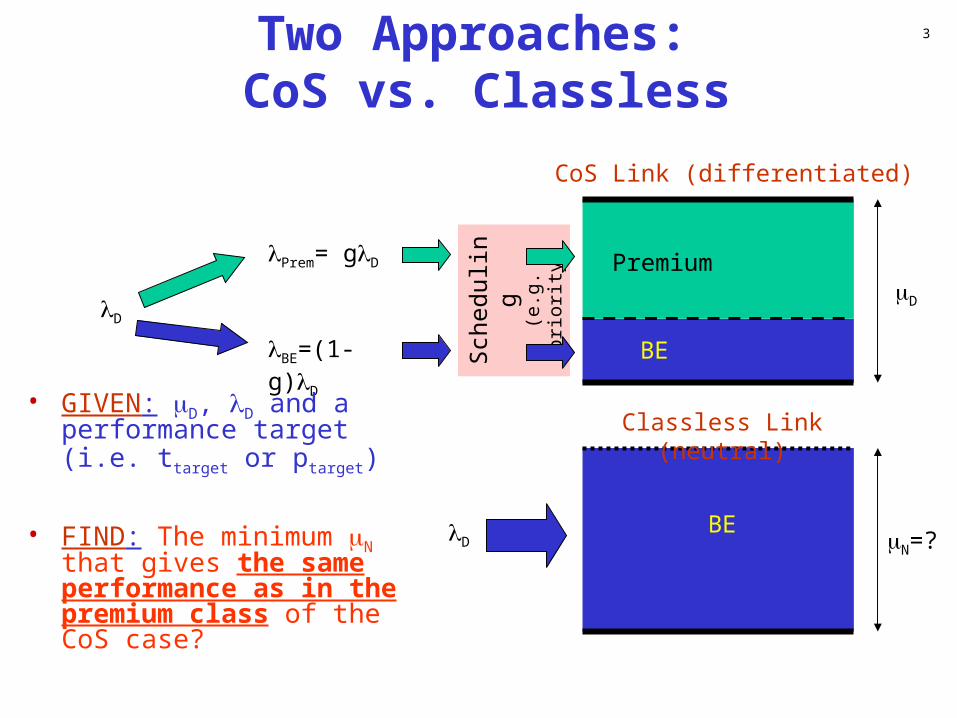
Two Approaches: CoS vs. Classless
Premium
BE
D
CoS Link (differentiated)
D
Prem= gD
BE=(1-g)D
D
• GIVEN: D, D and a performance target (i.e. ttarget or ptarget)
• FIND: The minimum N that gives the same performance as in the premium class of the CoS case?
N=?
Classless Link (neutral)
BE
Sch
edulin
g(e
.g.
pri
ori
ty)
3
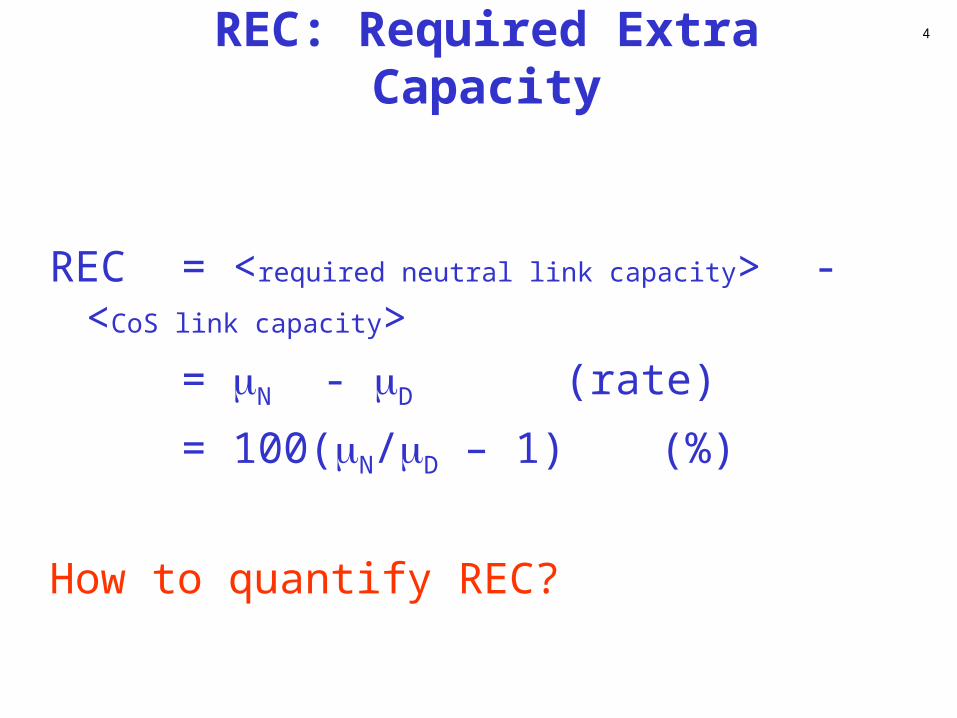
REC: Required Extra Capacity
REC = <required neutral link capacity> - <CoS link
capacity>= N - D (rate)
= 100(N/D – 1) (%)
How to quantify REC?
4
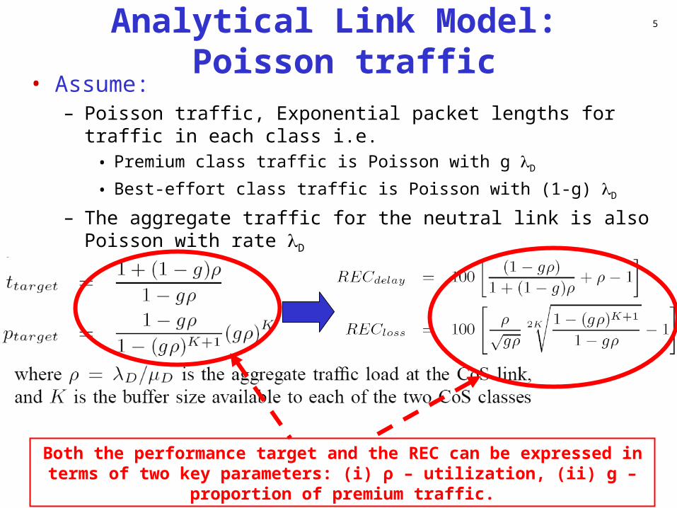
Analytical Link Model: Poisson traffic
• Assume:– Poisson traffic, Exponential packet lengths for traffic in each
class i.e.• Premium class traffic is Poisson with g D
• Best-effort class traffic is Poisson with (1-g) D
– The aggregate traffic for the neutral link is also Poisson with rate D
5
Both the performance target and the REC can be expressed in terms of two key parameters: (i) ρ – utilization, (ii) g – proportion of premium traffic.
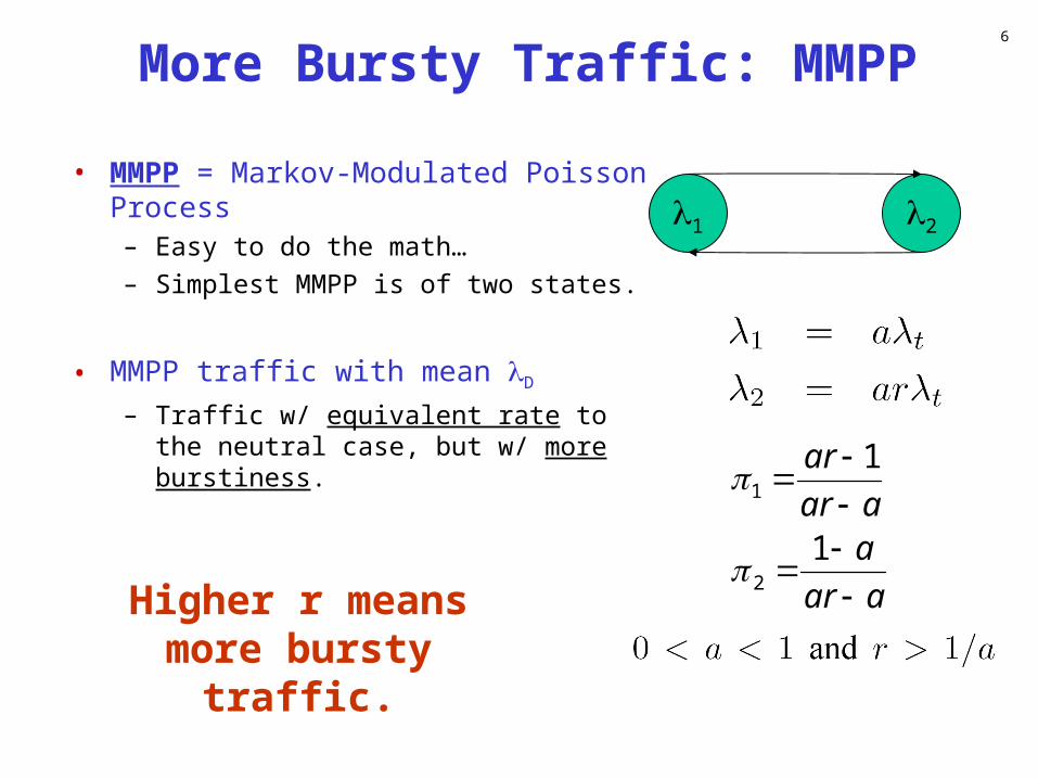
More Bursty Traffic: MMPP
• MMPP = Markov-Modulated Poisson Process– Easy to do the math…– Simplest MMPP is of two states.
• MMPP traffic with mean D
– Traffic w/ equivalent rate to the neutral case, but w/ more burstiness.
1 2
aar
aaar
ar
1
1
2
1
Higher r means more bursty
traffic.
6
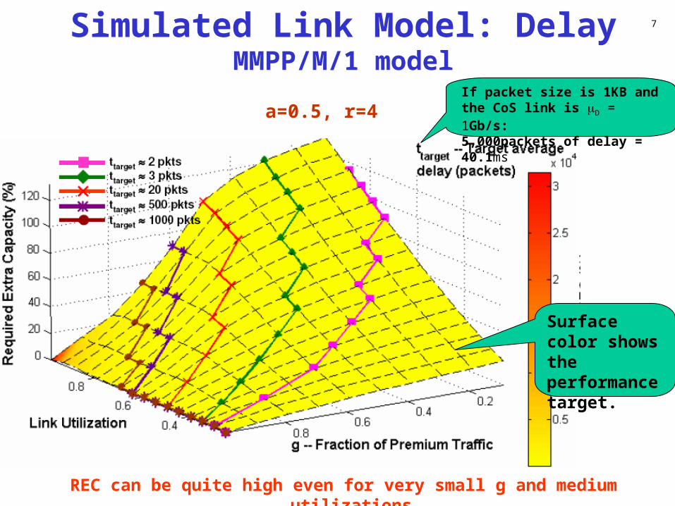
Simulated Link Model: DelayMMPP/M/1 model
a=0.5, r=4If packet size is 1KB and the CoS link is D = 1Gb/s:5,000packets of delay = 40.1ms
Surface color shows the performance target.
REC can be quite high even for very small g and medium utilizations.
7
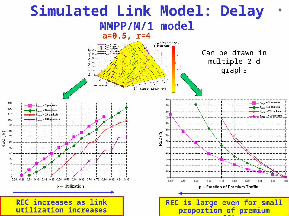
Simulated Link Model: DelayMMPP/M/1 model
a=0.5, r=4
REC increases as link utilization increases
REC is large even for small proportion of premium traffic
8
Can be drawn in multiple 2-d graphs

Simulated Link Model: LossMMPP/M/1/K model
The graphs are generic for various buffer sizes. An example: For a 10Mb/s link carrying 1KB packets:
K = ~15pkts 25ms buffer time
K = ~60pkts 100ms buffer time
9
REC for the same performance target decreases as buffer size increases
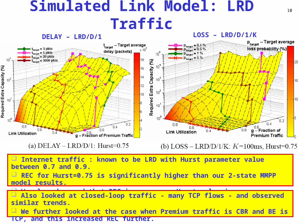
Simulated Link Model: LRD Traffic
10
Internet traffic : known to be LRD with Hurst parameter value between 0.7 and 0.9. REC for Hurst=0.75 is significantly higher than our 2-state MMPP model results. We also observed that REC increases as Hurst value increases towards 0.9.
DELAY – LRD/D/1 LOSS – LRD/D/1/K
Also looked at closed-loop traffic - many TCP flows - and observed similar trends. We further looked at the case when Premium traffic is CBR and BE is TCP, and this increased REC further.

Network Model
• Steps to calculate network REC (NREC):– Step 1: Construct the routing matrix RFxL based
on shortest path• Run Dijkstra’s algorithm on the topology
matrices ANxN and WNxN
– Step 2: Form the traffic vector Fx1 from TNxN
– Step 3: Calculate the traffic load on each link: RT = Q
– Step 4: Check the feasibility of the traffic load and routing
• For any link– If link capacity is less than the traffic load (e.g. C
< Q) then update T accordingly and go to Step 2.
– Step 5: Calculate the required per-link REC (i.e. N - D) by using QI as the traffic rate D for Ith link, and the performance goal ptarget or ttarget.
Used Rocketfuel
topologies for ANxN and WNxN.
Used gravity model for
TNxN.
Made a look-up to the simulated link model
results.
11
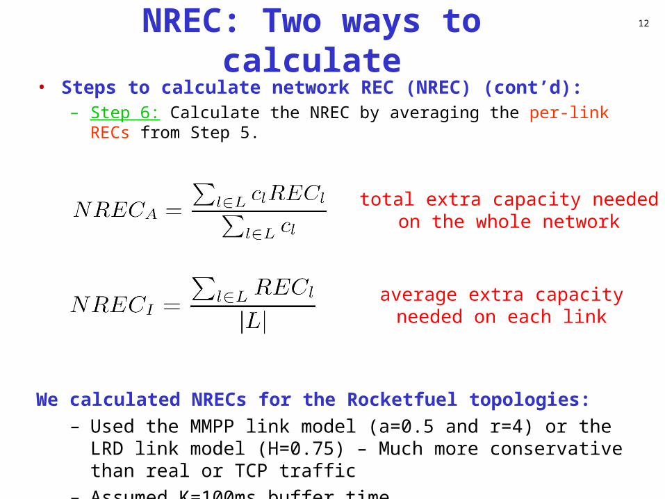
NREC: Two ways to calculate
• Steps to calculate network REC (NREC) (cont’d):– Step 6: Calculate the NREC by averaging the per-link RECs from
Step 5.
We calculated NRECs for the Rocketfuel topologies: – Used the MMPP link model (a=0.5 and r=4) or the LRD link
model (H=0.75) – Much more conservative than real or TCP traffic
– Assumed K=100ms buffer time– Only report Sprintlink, as the other topologies gave higher
REC values
12
total extra capacity needed on the whole network
average extra capacity needed on each link
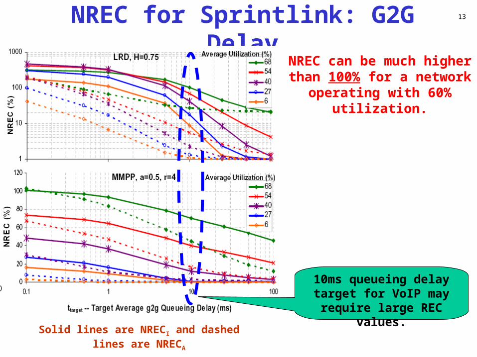
NREC for Sprintlink: G2G Delay
Solid lines are NRECI and dashed lines are NRECA
13
NREC can be much higher than 100% for a network
operating with 60% utilization.
10ms queueing delay target for VoIP may require large REC
values.

NREC for Sprintlink: G2G Loss
Solid lines are NRECI and dashed lines are NRECA
14
NREC can be much higher than 1000% even for a
network operating with 40% utilization.
0.1% loss target may require large REC
values.

Summary• A framework to study REC for delay or loss being the
performance target.• Link model
– REC grows when:• traffic becomes more bursty• the utilization of the CoS link becomes higher• the performance target becomes tighter• the fraction g of the Premium class traffic becomes smaller
– Closed-loop (e.g., TCP) or LRD traffic further increases REC
• Network model:– For legacy g2g performance targets, REC ranges from 50% to over
100% as g reduces below 0.5 and the utilization goes up to 60%.
• Future trends/work:– The performance targets will keep becoming tighter. REC is high
perpetually – not just today, but in future also.. – The value of g is a crucial factor. Small g does not necessary favor
a classless network.– Further research should estimate the actual costs of CoS and
classless designs, as scheduling & management complexity need to be considered.
15
Thank you!
THE END
16