quality sorting and trade: firm-level evidence for french …ies/fall07/mayerpaper.pdf · quality...

Quality sorting and trade:Firm-level evidence for French wine∗

Matthieu Crozet† Keith Head‡ Thierry Mayer§

October 31, 2007

Abstract

Investigations of the effect of quality differences on heterogeneous performancein exporting have been limited by lack of direct measures of quality. We examineexports of French wine, matching the exporting firms to producer ratings from twowine guidebooks. We show that high quality producers export to more markets,charge higher prices, and sell more in each market. Our model predicts qualitysorting: the more difficult a market is to serve, the better on average will be thefirms that serve it. Our findings point to the empirical importance of quality sortingin one industry and could be extended to other industries.

∗PRELIMINARY AND INCOMPLETE. We thank Isaac Holloway for research assistance and AndyBernard for very helpful suggestions.

†CEPII and University of Reims.‡Sauder School of Business, University of British Columbia, [email protected]§Universite de Paris I, Paris School of Economics, CEPII, and CEPR.

1 Introduction

Why do some firms export more intensively and extensively than others? In the seminalpapers of Melitz (2003) and Bernard, Eaton, Jenson, and Kortum (2003) the answeris productivity differences. However, measures of physical output per unit of input arerarely available at the firm level, forcing reliance on proxies like domestic market shares orvalue-added per worker. These variables can be driven by primitives other than physicalproductivity, such as product quality. A separate literature on quality and trade relies onnoisy proxies (unit values). We study French wine exports, where we are able to matchfirm-destination-level export flows to firm-level quality ratings from wine guides.

Prior work on quality and trade has examined both the supply side and demand side.Supply side research asks what makes a country export higher quality goods (as inferredfrom unit values)? Schott (2004) finds that within goods categories, unit values tend toincrease with the exporters’ per capita income, capital to labor ratio, skill ratio, and thecapital intensity of production. Hummels and Klenow (2005) find that, within categories,price and quantity indexes rise with origin-country income per capita. The elasticitiesare 0.09 (price) and 0.34 (quantity). The authors interpret their price result as showingwhy big countries do not suffer from a negative terms of trade effect (as they would in amodel without quality differentiation). Rather than drive down the value of their singlevariety, large countries export more varieties and also higher quantities and prices of eachvariety. Hummels and Klenow also argue in favour of a model with Romer (1994) fixedcosts per export market.

Demand-side papers ask what makes country demand a larger share of high qualitygoods (again inferred from unit values)? Hummels and Skiba (2004) find that averageFOB export price rise with freight costs to destination market. They interpret thisas a confirmation of the Alchian-Allen (1969) effect (“shipping the good apples out”).1

Hallak (2006) estimates destination-country income effects and find evidence supportingthe hypothesis that richer countries have relatively high demand for high quality. Hallakestimates an interaction between unit values (based on the US import data) and incomeper capita.2

This paper contributes to the quality and trade literature in terms of data and method.“Direct” quality measures compared to “inferred” quality (unit values, market shares).Firm-level quality measures matched to firm-level destination-specific exports. Our modelcombines the Hallak assumption on preferences for quality with the Baldwin and Harrigan(2007) assumption on the cost of quality. Methodologically, we develop new predictionsfor the heterogeneous quality model, relating conditional means to market attractivenessmeasures.

The paper proceeds as follows. We first derive new testable predictions from a model

1The Alchian-Allen effect relies upon freight costs that are less than proportional to product value.An increase in freight costs therefore lowers the relative price of high quality goods leading to an increasein their relative demand.

2The majority of the coefficients estimated are insignificant or negative and significant. Hallak’s“confirmation” of the theory is based upon finding more significant positive than significant negativecoefficients.

1

of firm-level heterogeneity in quality. Then we explain why applying this model to cham-pagne and burgundy producers makes sense. Next we estimate the firm-level equationsof that model and back out the implied values of the key structural parameters. Utilizingfixed effects estimated in the firm-level regressions, we estimate the conditional meanrelationships implied by the model. Our conclusion suggests a research program basedon the success of the quality sorting model as well as the empirical anomalies we find.

2 Theory

The theory examined in this paper is based on work by Baldwin and Harrigan (2007),who introduced a cost-quality tradeoff in the model of Melitz (2003), who introducedproductivity-heterogeneity in the model of Krugman (1980), who introduced trade coststo the monopolistic competition model of Dixit and Stiglitz (1977).

2.1 General Set-up

We consider a category of goods (in our case, an 8-digit goods classification) with a sub-utility function that is assumed to have a constant elasticity of substitution (CES), σ > 1,over the set, Bj, of all varieties, i available in country j:

Uj =

(∫i∈Bj

[s(i)γq(i)]σ−1

σ di

) σσ−1

. (1)

In this expression q(i) denotes quantity of variety i consumed and s(i) denotes its mea-sured quality.3 Following Hallak (2006), the intensity of the consumers’ desire for qualityis captured in parameter γ. The sub-utility enters full utility with a Cobb-Douglas ex-penditure parameter denoted µj. The foreign country comprises Mj individuals with yj

income per capita.Our data is based on export declarations which state values in FOB terms. Hence

we use x to denote FOB value of export and p = x/q to denote FOB prices. Exports ofvariety i to market j are given by

xj(i) =[pj(i)τj(i)/s(i)

γ]1−σ∫`∈Bj

[pj(`)τj(`)/s(`)γ]1−σd`µjyjMj/τj(i), (2)

In the above expression prices paid by consumers in j are given by pj(i)τj(i). Thus τj(i)−1is the ad valorem amount of all all trade costs incurred by firm i to sell in market j. As isstandard in the literature we assume a single factor of production, constant marginal costs,mill-pricing, the Dixit-Stiglitz markup, and iceberg transport costs. A firm is defined bythe trio of w(i), z(i), and s(i). Although we follow the convention of representing factorprices with w, we believe land is the more important factor for wine production. The

3In our application “star” ratings in wine guides provide s(i).

2

factor price is shown as firm-specific to capture the reality that firms have differing per-unit land costs. The productivity of the factor is denoted with z(i). Hence unit costs aregiven by w(i)/z(i). Since all our firms are located in close proximity to each other andprobably use the same transportation hubs, we approximate their trade costs as beingthe same for each market, τj. Taken together these assumptions imply export revenuefrom market j is given by

xj(i) =

(w(i)/z(i)

s(i)γ

)1−σ

µjyjMjτ1−σj P σ−1

j , (3)

where we have defined the price index in terms of quality-adjusted costs,

Pj ≡

(∫`∈Bj

[w(`)/z(`)

s(`)γ

]1−σ

d`

)1/(1−σ)

,

instead of prices so that the messy term involving the markup, [(σ− 1)/σ]σ−1 can cancelout in the numerator and denominator of (2).

The net contribution to firm profits of market j is given by

πj(i) = xj(i)/σ − F = ([z(i)/w(i)]s(i)γ)σ−1Aj/σ − F, (4)

where Aj is a factor that aggregates the determinants of the attractiveness of country jdefined as

Aj ≡ µjyjMj(τj/Pj)1−σ.

Attractiveness depends positively on the size (µjyjMj) of the market and relative access-ability (which is decreasing in τj/Pj).

2.2 The cost-quality tradeoff

We have so far allowed for heterogeneity in productivity (the standard approach followingMelitz (2003)), factor prices (an important consideration for wine producers), and quality.Three sources of heterogeneity is two too many for a tractable model. One option is tohold w/z constant and have a model of pure (costless) quality variation. The problemwith this is that in the Dixit-Stiglitz framework, mark-ups do not vary across firms andso quality has no independent effect on price. To account for the stylized fact that higherquality is associated with higher prices in this framework, we follow Baldwin and Harriganin assuming a deterministic tradeoff between cost and quality. We discuss the reasons toexpect such a relationship for wine in section 3.

Because we observe quality directly, and therefore want to focus on that variable, wemodify the parameterization of the cost-quality tradeoff slightly differently from Baldwinand Harrigan but this only matters for the exposition. Rather than assume firms draw aunit labour requirement (1/z), we assume firms draw a level of quality (s).

We assume that when firms take a high quality draw that a cost must be paid interms of higher factor prices and/or lower productivity. Thus we assume,

w(i)

z(i)= ωs(i)λ, (5)

3

with λ ≥ 0. Our parameter is related to the one used in Baldwin and Harrigan as follows:λ = 1/(1 + θ). For λ = 0, quality is costless and firms have unit factor costs given by ωno matter what quality they draw. Another useful special case is λ = −1. That value,combined with γ = 0 makes it possible to reinterpret s(i) as a productivity draw since itimplies w(i)/z(i) = ω/s(i). This allows us to compare the results of the quality-sortingmodel (γ > 0, λ ≥ 0) with the original Melitzian productivity sorting model (γ = 0,λ = −1).

2.3 Entry threshold quality

Substituting (5) into (4), we obtain

πj(i) = ω1−σs(i)(γ−λ)(σ−1)Aj/σ − F, (6)

For γ > λ, quality is valued at more than it costs to produce it, so a high s draw increasesprofits. Solving for the zero-profit cutoff quality for market j as

sj =

(Aj

σFωσ−1

) −1(σ−1)(γ−λ)

. (7)

As long as γ > λ it will be the case sj is the minimum level of quality required to entermarket j. This cut-off will be increasing in fixed costs and decreasing in the attractivenessof the market. For γ < λ, quality is not worth the cost and a lucky firm draws a low s.Thus, s becomes the maximum quality level.

If γ varies across countries then it is possible that, for some countries, s would be aminimum and, for others, it is a maximum. Hallak (2006) assumes a positive semi-logrelationship between per-capita income and the intensity of preference for quality:

γj = γ0 + γ1 ln(yj/y0), (8)

with γ1 > 0. Hallak’s original specification did not include y0. In his model γ0 is theintensity of preference for a hypothetical country with yj = 1. In our specification γj = γ0

for yj = y0. By setting y0 = to the world average we obtain a convenient interpretationfor estimates of γ0.

For quality to be desirable for exporting to market j—and therefore for sj to representa minimum—it must be that ln yj > ln y0 + (λ − γ0)/γ1. We assume for the purposesof calculating conditional expectations that this condition is met for all j but we willreconsider when we look at the data.

When this condition is met, the interpretation of (7) is straightforward. The level ofquality needed to enter market j is a negative function of how “easy” this market is forFrench exporters, which is captured by Aj. On the contrary, higher costs, either fixed(F ) or variable (ω) increase the quality cut-off, which means that lower quality firms willnot be able to sell abroad. This is for the quality draw model. Note that the logic isthe same in the efficiency draw case, where γ = 0 and λ = −1. In the ED model, theproductivity cut-off level decreases with ease of market Aj and increases with costs.

4

To obtain closed form solutions, we follow much of the recent literature in assuming aPareto distribution for heterogeneity. Thus, assume that the CDF, G(s), and PDF, g(s),take the forms

G(s) = 1− (s/s)−κ, and g(s) = κsκs−κ−1. (9)

The total pool of firms that might export to market j is given by Nx, which we consideras an exogenous variable here. The share of firms exporting to a market j is

Nj/Nx = Pr(s > s) = 1−G(s) = (s/s)−κ. (10)

Plugging in equation (7) for sj we can express the number of exporters to a market as afunction of the attributes of the market.

Nj = Nx

(Aj

σFωσ−1

) κ(σ−1)(γ−λ)

sκ (11)

The variable Aj collects a potentially large set of variables, some of which (e.g. tradecosts) are difficult to measure. An alternative approach is invert equation (10) to expressthe critical entry threshold as a function of the number of entrants:

sj = G−1(1−Nj/N) = (Nj/Nx)−1/κs (12)

In this formulation Nj/Nx can be thought of a single index of the ease of entering marketj. This has the advantage of compactness, and will be useful in particular as a graphicaldevice. We will also however present results in terms of the primitives of the model, and inparticular Aj and its underlying components, for testing models’ predictions in regressionanalysis, using (7) rather than (12). We now proceed to detailing those predictions interms of measurable aggregate statistics: the average quality, average price and averagequantity on each destination market j.

2.4 Conditional mean quality

The average quality of exporters to a given market is E[s | s > s]. The general form forthe expected value of a variable truncated from below is

E[s | s > s] =1

1−G(s)

∫ ∞

s

sg(s)ds.

The expected value of a truncated Pareto is

E[s | s > s] = sκ

κ− 1. (13)

Then substituting (12) into equation (13), we remove the unobserved threshold and obtainthe observed conditional mean quality of exporters to a market as a function of theobserved number of exporters to that market

E[s | s > s] =

(Nj

Nx

)−1/κ

sκ

κ− 1(14)

5

This negative relationship between average quality and popularity presumes truncationfrom below, which occurs for sufficiently high income countries, the ones that place im-portance on quality.

To obtain the prediction in terms of the primitives, substitute (7) into equation (13),and obtain

E[s | s > s] =

(Aj

σFωσ−1

) −1(σ−1)(γ−λ) κ

κ− 1(15)

The testable predictions are straightforward. Anything that makes a market moreattractive (higher Aj) will reduce the average level of quality (in the QD model) or theaverage level of productivity (in the ED model) measured for exporters to market j. Ina reduced form equation Aj can be approximated as a positive function of market sizeand a negative function of distance (or any other measurable proxy for trade costs toj). Average performance (quality or efficiency) of French exporters in j should thereforedecrease with GDP in j and increase with distance to j. Note that if fixed costs werealso a function of distance, it should be a positive one, and the overall prediction isunchanged: more distant markets should exhibit higher average performance (quality orefficiency). Assessing which type of sorting is actually taking place requires measures ofindividual quality and efficiency, which is not always available. There are, however, somediscriminating predictions between the two models to which we now turn.

2.5 Conditional mean price

With Dixit-Stiglitz pricing behavior and the cost-quality relationship embodied in equa-tion (5), individual firms charge FOB prices of

pj(i) =σ

σ − 1ωs(i)λ. (16)

These prices do not vary across destination markets. A more general model mightincorporate such variation either via cross-country differences in σ, and hence the mark-up. The mean price conditional on exporting does vary across markets:

E[p | s > s] =1

1−G(s)

∫ ∞

s

p(s)g(s)ds =ωσ

(σ − 1)(1−G(s))

∫ ∞

s

sλg(s)ds. (17)

Evaluating this expression for a Pareto distribution, we obtain4

E[p | s > s] =sλωσκ

(σ − 1)(κ− λ). (18)

Using equation (12) to substitute out the unobservable s we obtain

E[p | s > s] =

(Nj

Nx

)−λ/κsλωσκ

(σ − 1)(κ− λ). (19)

4For the integral to be finite we need κ > λ.

6

As with mean quality, the mean price conditional on exporting is decreasing in Nj/Nx

for the QD model. However, the prediction is opposite for the ED model, which youobtain by setting γ = 0 and λ = −1. When quality sorting takes place, only high qualityvarieties get exported to difficult countries, and those are high price varieties, becausehigh quality is associated with high costs in our setting. When efficiency sorting is thedriver of firms’ selection into export markets, only the most productive firms with lowmarginal cost make it to difficult markets, and -with a constant markup- those have alow price.

In terms of the primitives, the prediction on average price is the following:

E[p | s > s] =

(Aj

σF

) −λ(σ−1)(γ−λ) ω

γ(γ−λ) σκ

(σ − 1)(κ− λ). (20)

Recall that attractiveness, Aj ≡ µjyjMjτ1−σj P σ−1

j . In the QD model, where γ > λ > 0,the average price should therefore be a negative function of population (Mj), income percapita yj and taste for wine µj. It should however be increasing in distance dj, whichenters τj (and possibly Fj) positively. A reduced form equation of the QD model can beestimated in the following form:

ln E[p | s > s] = α0 + α1 ln Mj + α2 ln yj + α3 ln dj + εj, (21)

where α1, α2 < 0 and α3 > 0. This is a reduced form equation since i) not all componentsof trade costs are controlled for, ii) the fixed cost is left constant5, iii) the unobservablepreference parameter µj and price index Pj are left in the disturbance term. The EDmodel calls for opposite coefficients on all those variables, enabling for a discriminatingtest between those two views of exporters’ sorting.

2.6 Conditional mean quantity exported

Exports of variety i, expressed as a function of quality are given by

xj(i) = ω1−σAjs(i)(γ−λ)(σ−1) (22)

The quantity exported by a firm with quality s can be obtained by dividing (22) by theequation for FOB prices, (16):

qj(i) =σ − 1

σω−σAjs(i)

(σ−1)γ−λσ (23)

The conditional mean quantity is therefore given by

E[q | s > s] =σ − 1

σ

ω−σAj

1−G(s)

∫ ∞

s

s(σ−1)γ−λσg(s)ds. (24)

5As mentioned above however, if fixed costs of serving j are increasing in distance dj , the predictionon the signs of coefficients is left unaffected.

7

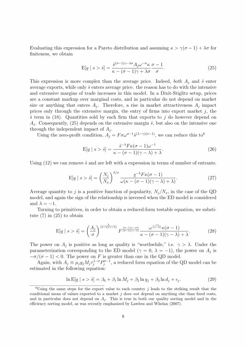
Evaluating this expression for a Pareto distribution and assuming κ > γ(σ − 1) + λσ forfiniteness, we obtain

E[q | s > s] =s(σ−1)γ−λσAjω

−σκ

κ− (σ − 1)γ + λσ

σ − 1

σ. (25)

This expression is more complex than the average price. Indeed, both Aj and s enteraverage exports, while only s enters average price. the reason has to do with the intensiveand extensive margins of trade increases in this model. In a Dixit-Stiglitz setup, pricesare a constant markup over marginal costs, and in particular do not depend on marketsize or anything that enters Aj. Therefore, a rise in market attractiveness Aj impactprices only through the extensive margin, the entry of firms into export market j, thes term in (18). Quantities sold by each firm that exports to j do however depend onAj. Consequently, (25) depends on the extensive margin s, but also on the intensive onethrough the independent impact of Aj.

Using the zero-profit condition, Aj = Fσωσ−1s(λ−γ)(σ−1), we can reduce this to6

E[q | s > s] =s−λFκ(σ − 1)ω−1

κ− (σ − 1)(γ − λ) + λ. (26)

Using (12) we can remove s and are left with a expression in terms of number of entrants.

E[q | s > s] =

(Nj

Nx

)λ/κs−λFκ(σ − 1)

ω(κ− (σ − 1)(γ − λ) + λ). (27)

Average quantity to j is a positive function of popularity, Nj/Nx, in the case of the QDmodel, and again the sign of the relationship is inversed when the ED model is consideredand λ = −1.

Turning to primitives, in order to obtain a reduced-form testable equation, we substi-tute (7) in (25) to obtain

E[q | s > s] =

(Aj

σ

) λ(σ−1)(γ−λ)

F(σ−1)γ−σλ(σ−1)(γ−λ)

ω−γ

(γ−λ) κ(σ − 1)

κ− (σ − 1)(γ − λ) + λ. (28)

The power on Aj is positive as long as quality is “worthwhile,” i.e. γ > λ. Under theparameterization corresponding to the ED model (γ = 0, λ = −1), the power on Aj is−σ/(σ − 1) < 0. The power on F is greater than one in the QD model.

Again, with Aj ≡ µjyjMjτ1−σj P σ−1

j , a reduced form equation of the QD model can beestimated in the following equation:

ln E[q | s > s] = β0 + β1 ln Mj + β2 ln yj + β3 ln dj + εj. (29)

6Using the same steps for the export value to each country j leads to the striking result that theconditional mean of values exported to a market j does not depend on anything else than fixed costs,and in particular does not depend on Aj . This is true in both our quality sorting model and in theefficiency sorting model, as was recently emphasized by Lawless and Whelan (2007).

8

When F does not vary across countries, the prediction is very simple and opposite tothe one on prices: β1, β2 > 0 and β3 < 0. This is a reduced form equation for the samereasons as the price equation. Again, the ED model calls for opposite coefficients on allthose variables, enabling for a discriminating test between those two views of exporters’sorting. In the QD model, easy markets see lower quality firms on average export highquantities of low price goods. In the ED case, those same high Aj countries face exportsby less efficient firms on average that charge high prices and sell less.

There appears to some ambiguity regarding the F term. Suppose that Fj is a positivefunction of dj. In the average price equation, the sign prediction on α3 is unchanged sinceτj and Fj are raised to the same power in (20). This is not the case in the mean quantityequation (28) since (σ − 1)γ − σλ > 0 as long as γ > λ > 0 and σ > 1. In that case, dj

has a positive influence on average quantity through Fj and a negative one through τj

in Aj. Note that in the ED parameterization, the distance should unambiguously raiseaverage quantity.

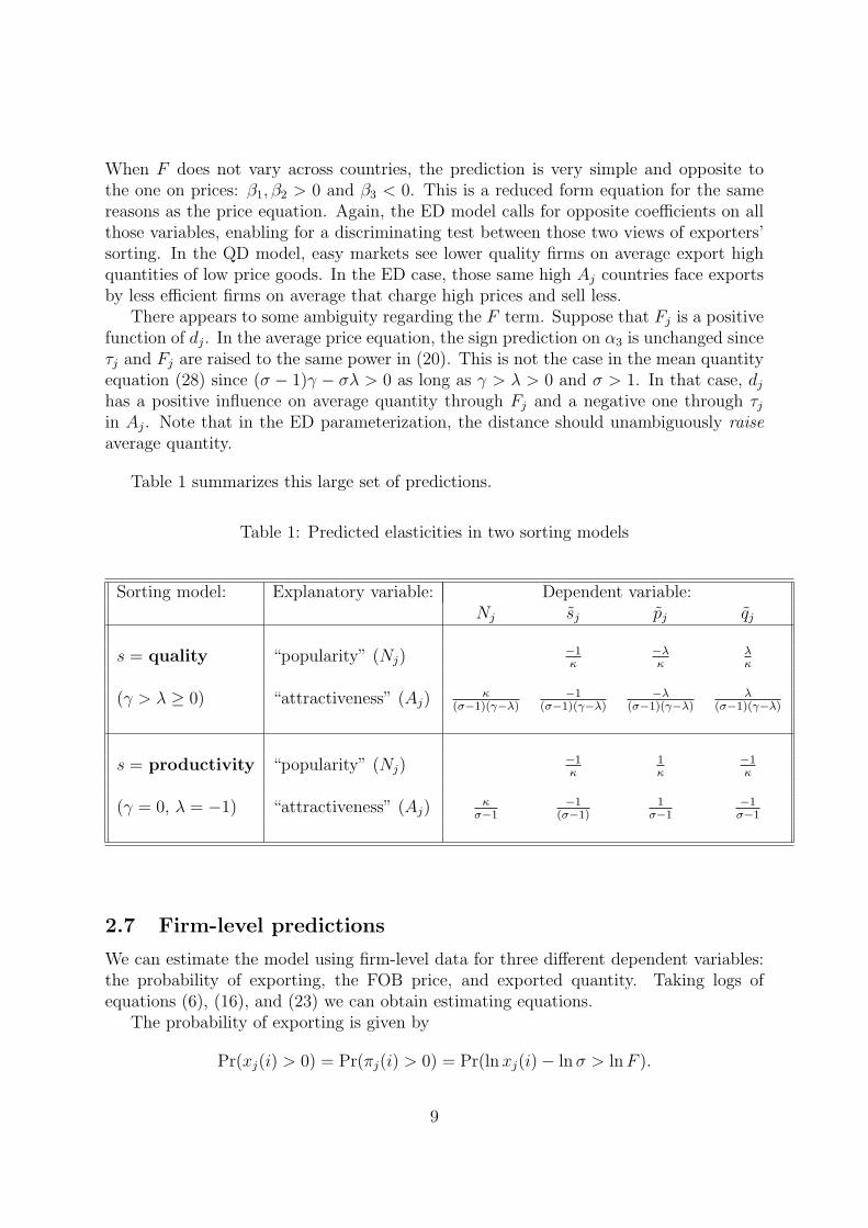
Table 1 summarizes this large set of predictions.

Table 1: Predicted elasticities in two sorting models

Sorting model: Explanatory variable: Dependent variable:Nj sj pj qj

s = quality “popularity” (Nj)−1κ

−λκ

λκ

(γ > λ ≥ 0) “attractiveness” (Aj)κ

(σ−1)(γ−λ)−1

(σ−1)(γ−λ)−λ

(σ−1)(γ−λ)λ

(σ−1)(γ−λ)

s = productivity “popularity” (Nj)−1κ

1κ

−1κ

(γ = 0, λ = −1) “attractiveness” (Aj)κ

σ−1−1

(σ−1)1

σ−1−1σ−1

2.7 Firm-level predictions

We can estimate the model using firm-level data for three different dependent variables:the probability of exporting, the FOB price, and exported quantity. Taking logs ofequations (6), (16), and (23) we can obtain estimating equations.

The probability of exporting is given by

Pr(xj(i) > 0) = Pr(πj(i) > 0) = Pr(ln xj(i)− ln σ > ln F ).

9

Without some additional source of heterogeneity, this probability would be one for s(i) >sj and zero otherwise. One way of introducing firm-level uncertainty is to assume thatthe fixed costs of exporting to country j for firm i, Fj(i) vary depending on a commoncomponent f , and a firm-country unobservable term εj(i). From (6), firm i will exportto j with probability:

Pr(xj(i) > 0) = Pr[(1− σ) ln(ω/fσ) + ln Aj + (γ − λ)(σ − 1) ln s(i) > εj(i)]. (30)

The parameters of this probability can be estimated by probit or logit depending on theassumption made on the distribution of the error term εj(i). We use logit because it canabsorb the country-year fixed effects for the Aj.

7

From (16), the price charged by firm i takes the following estimable form:

ln pj(i) = ln[σ/(σ − 1)] + ln ω + λ ln s(i), (31)

From (23), the firm-level exported quantity is

ln qj(i) = ln[(σ − 1)/σ]− σ ln ω + ln Aj + [(γ − λ)(σ − 1)− λ] ln s(i). (32)

For export probabilities and quantities, ln Aj appears on the RHS. Rather than at-tempt to estimate this term as a parametric function of country j primitives, we absorb itwith country-year-specific fixed effects. Firm-level prices do not vary across destinationsin the model but it is natural to relax the strong assumption of non-varying σ. In thatcase the structural interpretation of the country level fixed effect in the price equation isln[σj/(σj − 1)].

We have also estimated a semi-parametric form of these regressions in which we replaceln s(i) with a set of indicator variables corresponding to the number of stars accorded tothe producer. Our initial assessment was that the gain from more flexibility was not highenough to offset the cost in terms of the inability to extract estimates of γ and λ and thegreater number of coefficients to report and discuss.

3 Why Wine?

Champagne (nc8 22041011) and red burgundy (nc8 22042143) have built reputations fornon-replicable attributes. Thus, they exhibit Armington-style differentiation by place oforigin. With Champagne this is an organized legal and promotional effort. To qualify aschampagne in the EU (and Canada), a wine must be produced within the Champagnegeographic appelation.

“The important thing to remember is that while some processes of Champagneproduction may be duplicated, the terroir is unique, original, and impossibleto replicate.” (www.champagne.us)

7The Stata command is “xtlogit, fe”

10

www.champagne.us

Some wine critics agree with the proposition that sparking wine from Champagne isdistinct:

“The Champagne region has certain natural advantages that no amount ofmoney, ambition, or talent can surmount: The combination of chalky soil andfickle northern European weather yields sparkling wines that simply can’t bereplicated anyplace else, or at least anyplace that’s been tried.” (Steinberger,2005)

Burgundy producers do not invest in such overt promotion of their regional identity.However, wine critics tend to judge pinot noir wines relative to the Burgundian style.Furthermore, the most expensive wines in the world are red burgundies.

The relevance for this study is that Melitz (2003) model, upon which we base ouranalysis, assumes that firms face only the option of exporting or not to a given market.They cannot relocate production as in the Helpman, Melitz, Yeaple (2004) framework.With footloose production, the implications for quality sorting could be quite different.Thus, the geographic definition of champagne and burgundy makes these goods particu-larly appropriate for studying the effect of heterogeneity on the composition of exportersby destination.

While the model rests upon a product that is not reproducible in the export mar-ket, it also insists on firm-level differentiation within each country. Champagne fits thisassumption well. Geographic distinctions within champagne region (a single appelation)are not emphasized.

“[E]ssence of champagne is that it is a blended wine, known in all but ahandful of cases by the name of the maker, not the vineyard.” (Johnson andRobinson, 2005)

Quality determined by cellar-master’s talent at blending, “dosing,” etc. Sales policyemphasizes the brand.

In Burgundy, on the other hand, there are many small appelations, each of which issupposed to have distinct properties. Within the appelations, vineyards are further strat-ified into village wines, premier cru and grand cru. Many different producers typicallymake wine from grapes from the same grand cru vineyard. Conversely most producershave obtain grapes from multiple vineyards. Burgundians attribute most quality varia-tion to place-specific terroir : the soil, topography, and microclimate. Comparing acrosswines from the same vineyard, they also emphasize vintage: year-specific weather. Sinceour data does not report the vineyard or the vintage of the wine exported, it would ap-pear ill-suited to capture quality variation in burgundy wine. However, Robert Parker,the most influential wine critic in the world, asserts that there are large within-vineyardquality differences due to firm-specific variation in viticulture and vinification practices.

“Knowing the finest producers in Burgundy is unquestionably the most im-portant factor in your success in finding the best wines.”

11

There are several mechanisms supporting a cost-quality tradeoff in wine. First thereis the cost of acquiring land with the desirable terroir properties. In Burgundy “villagevineyards” cost e150–500K/ha (Robinson, 20??). Assuming an interest rate of 5% anda typical yield of 5000 bottles per hectare, this corresponds to a unit land cost of e1.5–5per bottle. On the other hand, land that has been designated as a grand cru vineyardcosts over e2M/ha, or more than e20 per bottle. In the Champagne region the major,where the quality of land has been built into the price of grapes through the system calledechelle des crus. Thus if we think of w(s) as the factor costs embodied in wine of qualitys, we have good reasons to expect w′ > 0.

Wine is also believed to exhibit a trade-off between yield and quality. Low-yield viti-culture, which involves pruning back vines from 40 hectalitres per hectare (the averagein Burgundy) to 20 hl/ha (the yield at the Romanee Conti vineyard) doubles unit landcosts. However, Parker and most other wine experts argue that this raises flavour con-centration. Indeed the importance of yield is recognized in much of the AOC regulationin France which sets allowable yield levels by appelation.

The process of winemaking itself also exhibits cost-quality tradeoffs. One familiarexample is the use of new oak barrel. The advantage of new oak is that imparts moreflavour into the wine. However, our calclations indicate that it adds something in theneighborhood of e2 to the cost of each bottle.

4 Data

4.1 Trade data

We use the micro-data collected each year based on export declarations submitted toFrench Customs. It is an almost comprehensive database which reports annual individ-ual shipments of each French exporting firms. The “almost” is due to EU legislationfollowing the implementation of the single market, which set different thresholds for com-pulsory declarations inside and outside the customs union. Inside the EU, shipmentsare reported if their annual trade value exceeds 250,000 euro. Exports outside the EUare recorded unless their value is smaller than 1000 euros or one ton. For each firm,Customs records values and quantities exported to 216 importing countries, and 11,5788-digit product classifications (combined nomenclature, which is abbreviated as “nc8”).We have observations for the six years from 1998 to 2003.

The nc8 is the harmonized system 6-digit (hs6) code with a 2-digit suffix that isparticular to the European Union. Wine has hs4 of 2204. Sparkling wine is 220410 andstill red wine less in less than two liter containers is 220421. For our purposes is fortunatethat the last two digits of nc8 distinguish important wine-growing regions in the EU. Thuschampagne, the sparkling wines of the official Champagne region are recorded as nc8 #22041011. Furthermore, red wines from the Burgundy wine region is classified as nc8 #22042143.

Champagne and red burgundy account for 0.45% and 0.048% respectively of Frenchmanufacturing trade. This might not seem much per se, but it is rather large compared

12

to other industries. The mean industry-level contribution to total trade is less than 0.01%and the largest exporting industry (aeroplanes and other aircraft exceeding 15 tons) ac-counts for 3.24% only. Our two industries are clearly among the largest 5% of contributorsto French trade. They also are strong outliers in other dimensions. When ranking nc8products according to number of exporting firms, champagne and red burgundy rank 21stand 65th respectively out of 11,578 products. Their importance is even more striking interms of the number of destination countries. As figure 1 shows, those two industriesexport to a much larger number of countries than the typical French industry.

Number of destination markets (average per year)

prob

abili

ty d

ensi

ty

0.00

00.

005

0.01

00.

015

0.02

00.

025

0 25 50 75 100 125 150 1750

500

1000

1500

freq

uenc

y

Exponential PDF

ChampagneRed Burgundy

Figure 1: Champagne and Wine are outliers in the distribution of destinations per product

The export declaration data provided us with firm identification numbers, or SIREN,for all 12,314 firms who exported any form of wine (hs4 = 2204) between 1998 and 2003.Of those, the French National institute (INSEE) provided us with the names, addresses,principal industry code, and other attributes of 10,341 firms in existence as of June 2007.We used the firm-level information to match our exporters with wine producers that wererated in two guidebooks.

4.2 Quality ratings

Wine producer quality ratings come from two different sources: i) a French one: Burtschy,Bernard and Antoine Gerbelle, 2006, Classement des meilleurs vins de France, Revue Des

13

Vins De France (Paris), which we will refer to as RVF, ii) an internationally recognizedone: Parker, Robert, Wine Buyer’s Guide, 5th Edition, 1999, which we refer to as WBG.For each of the listed producers, the name and location were matched with the exporter’sdataset by hand.

In RVF, listed producers receive between 0 and 3 stars. We have 64 champagneproducers listed, and are able to match those with 51 exporters. For burgundy, 268 arelisted, of which 206 can be found in the customs dataset. In WBG, producers (70 forchampagne, and 159 for burgundy) are categorized as “average,” “good,” “excellent,” or“outstanding.” Of those we manage to find 47 champagne exporters and 139 burgundyexporters.

Table 2: Champagne quality ratingsRVF’s Classement

Parker’s WBG n/a Incl. * ** *** Totaln/a 1724 16 6 0 0 1746Average 3 1 0 0 0 4Good 7 3 1 2 0 13Excellent 7 6 4 3 0 20Outstanding 1 0 3 4 2 10Total 1742 26 14 9 2 1793Note: Kendall’s τ measure of concordance −1 ≤ τ ≤ 1

(p-value for test for independence), all exporters:0.58 (0.000) / included in both books: 0.43(0.009).

Table 3: Burgundy quality ratingsRVF’s Classement

Parker’s WBG n/a Incl. * ** *** Totaln/a 1389 69 44 20 4 1526Average 19 7 6 4 1 37Good 28 4 4 12 1 49Excellent 11 1 11 14 1 38Outstanding 4 1 4 3 3 15Total 1451 82 69 53 10 1665Note: Kendall’s τ measure of concordance −1 ≤ τ ≤ 1

(p-value for test for independence), all exporters:0.39 (0.000) / Included in both books: 0.22(0.023).

Customs data lists exports by a firm for each nc8 product. However, in other firm-levelsources of data, firms are classified according to a“primary” activity. It appears actually

14

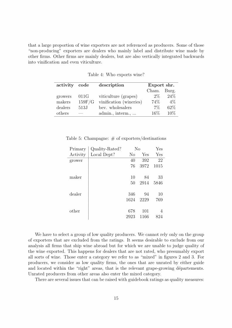
that a large proportion of wine exporters are not referenced as producers. Some of those“non-producing” exporters are dealers who mainly label and distribute wine made byother firms. Other firms are mainly dealers, but are also vertically integrated backwardsinto vinification and even viticulture.

Table 4: Who exports wine?

activity code description Export shr.Cham. Burg.

growers 011G viticulture (grapes) 2% 24%makers 159F/G vinification (wineries) 74% 4%dealers 513J bev. wholesalers 7% 62%others — admin., interm., ... 16% 10%

Table 5: Champagne: # of exporters/destinations

Primary Quality-Rated? No YesActivity Local Dept? No Yes Yesgrower 40 392 22

76 3972 1015

maker 10 84 3350 2914 5846

dealer 346 94 101624 2229 769

other 678 101 42923 1166 824

We have to select a group of low quality producers. We cannot rely only on the groupof exporters that are excluded from the ratings. It seems desirable to exclude from ouranalysis all firms that ship wine abroad but for which we are unable to judge quality ofthe wine exported. This happens for dealers that are not rated, who presumably exportall sorts of wine. Those enter a category we refer to as “mixed” in figures 2 and 3. Forproducers, we consider as low quality firms, the ones that are unrated by either guideand located within the “right” areas, that is the relevant grape-growing departements.Unrated producers from other areas also enter the mixed category.

There are several issues that can be raised with guidebook ratings as quality measures:

15

Figure 2: Markets/firm

(a) RVF rating: Champagne (b) WBG rating: Champagne

1 2 5 10 20 50 100

0.00

20.

010

0.05

00.

200

1.00

0

number (k) of markets (log scale)

shar

e of

firm

s ex

port

ing

to k

or

mor

e (lo

g sc

ale)

●

●

●

●

●●

●●

●●●●●

●●●●●

●

●

●

●

●●

●

●●●●

●

●

●

●●

●●

●●

●

●

●

●

●

●

Quality Rating

******includedlowmixed

1 2 5 10 20 50 100

0.00

20.

010

0.05

00.

200

1.00

0


shar

e of

firm

s ex

port

ing

to k

or

mor

e (lo

g sc

ale)

●

●

●

●

●

●

●

●

●●

●●

●●●

●

●

●

●●

●●

●●

●●●●

●●

●

●

●●●

●●

●●●

●

●

●

●

Quality Rating

outstandingexcellentgoodaveragelowmixed

(c) RVF rating: Burgundy (d) WBG rating: Burgundy

1 2 5 10 20 50 100

0.00

20.

010

0.05

00.

200

1.00

0


shar

e of

firm

s ex

port

ing

to k

or

mor

e (lo

g sc

ale)

●

●

●

●

●●

●

●

●●

●

●

●

●

●

●

●

●●

●●

●●

●●

●●

●●

●

●

●

●●

●●

●

●●

●●

●●●●●●●

●

●

●

●●

●●●

●

●

●

●

Quality Rating

******includedlowmixed

1 2 5 10 20 50 100

0.00

20.

010

0.05

00.

200

1.00

0


shar

e of

firm

s ex

port

ing

to k

or

mor

e (lo

g sc

ale)

●

●

●

●

●●

●

●●

●●

●

●

●

●●

●●

●●

●

●

●

●

●

●●

●●

●●●●

●●●●●●●●●

●

●

●

●●

●●●●

●

●

●

●

Quality Rating

outstandingexcellentgoodaveragelowmixed

16

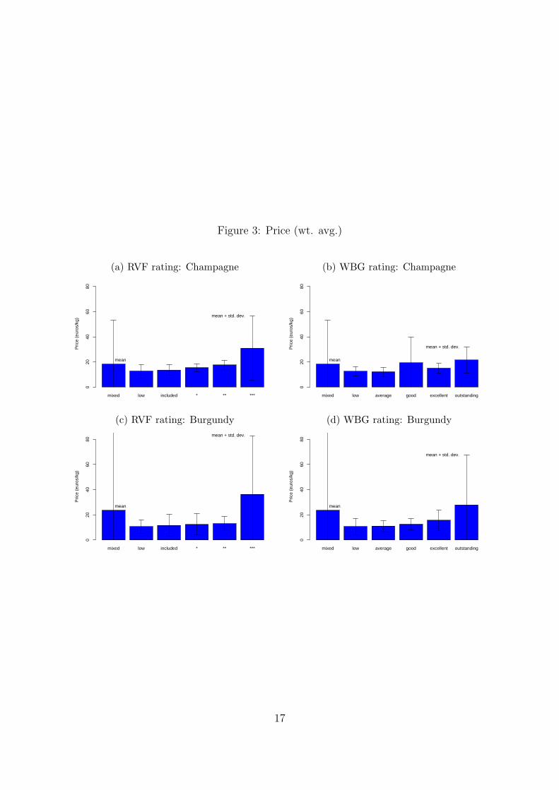
Figure 3: Price (wt. avg.)

(a) RVF rating: Champagne (b) WBG rating: Champagne

mixed low included * ** ***

Pric

e (e

uros

/kg)

020

4060

80

mean

mean + std. dev.

mixed low average good excellent outstanding

Pric

e (e

uros

/kg)

020

4060

80

mean

mean + std. dev.

(c) RVF rating: Burgundy (d) WBG rating: Burgundy

mixed low included * ** ***

Pric

e (e

uros

/kg)

020

4060

80

mean

mean + std. dev.

mixed low average good excellent outstanding

Pric

e (e

uros

/kg)

020

4060

80

mean

mean + std. dev.

17

Table 6: Burgundy: # exporters/destinations

Primary Quality-Rated? No YesActivity Local Dept? No Yes No Yesgrower 91 303 1 170

175 3276 2 4554

maker 21 20 5136 482 182

dealer 298 157 6 621922 3739 98 3159

other 356 143 2 301346 1112 54 643

1. The ratings are hard to interpret : units of measurement (stars) do not correspondto prices or quantities. Our theory includes parameter to measure marginal utilityof quality units. This parametric approach also has the advantage of compactnessin results presentation.

2. The ratings are unreliable: authors may have idiosyncratic tastes or be influenced bynon-taste considerations.8 In order to minimize this concern, we use two completelyindependent sets of ratings, for which we have no reason to suspect that author-specific “specificities” would be correlated.

3. The ratings are incomplete: bad producers are usually omitted from the guidebooksand much wine is exported by non-producers. We try to correct for this by inferringthe set of low quality firms and eliminating firms likely to have mixed quality.

4. The ratings may influence price directly : Some wine experts have become so famousworldwide, that their opinion exerts a direct impact on the price a firm can chargefor its wine.

5. The ratings may influence demand by increasing foreign customer awareness. Forinstance, consumers in New Zealand are probably not aware of all varieties of redburgundy produced and available for consumption in France. A guide like Parker’s,because it is in English, and so widely popular will change to effective set of varietiesin the consumer’s information set. To eliminate this concern, we run a separate setof regressions using only the French guide ratings (RVF) and restricting the sampleto non-francophone markets (RVF is not translated).

8Parker and the Faiveley affair.

18

5 Results

We start by presenting results on our firm-level predictions about how quality affects theprobability to become an exporter, quantity shipped and price charged.

5.1 Individual level analysis

Tables 7, 8, 9, and 10 report results of our firm-level regressions. In each of those tables,the first three columns average the two quality ratings (WBG and RVF) when measurings(i). The last three columns uses only the French rating (RVF) and restricts the sampleto non-francophone countries.

Table 7: Champagne firm-level regressions

(1) (2) (3) (4) (5) (6)qjt(i) > 0 ln pjt(i) ln qjt(i) qjt(i) > 0 ln pjt(i) ln qjt(i)

ln s(i) 3.61a 0.29a 1.80a 3.23a 0.25a 1.24a

(0.03) (0.01) (0.03) (0.03) (0.01) (0.04)

constant 2.50a 6.22a 2.59a 6.87a

(0.01) (0.03) (0.01) (0.03)Ratings WBG & RVF average RVF onlyDestinations all markets non-francophone marketsObservations 405189 12426 12426 317516 8801 8801Within-jt R2 0.117 0.203 0.092 0.102ρ: frac. var. ∼ FE 0.38 0.29 0.37 0.25

Destination-year (jt) fixed effects. Standard errors in parentheses.Significance levels: c p < 0.1, b p < 0.05, a p < 0.01

These regressions can be used to reveal the structural parameters of the model. Recallthat equation (32) defines the elasticity of quantity with respect to quality as ηqs ≡(γ − λ)(σ− 1)− λ. Therefore, the implied value of γ is λ + (ηqs + λ)/(σ− 1). Parameterλ can be obtained as the coefficient on log quality in the price regression, 0.29. Andersonand van Wincoop (2004) report 5 ≤ σ ≤ 10 as a reasonable range for the CES. Pluggingin estimates obtained for the full sample, we infer γ to lie between 0.52 and 0.81. Usingthe higher of the two values, a consumer is willing to trade 3.7 bottles of low quality(s = 1) wine for one bottle of the highest quality (s = 5).

Furthermore, we can use estimates in Table 8 to test the Hallak (2006) assumption ofincome dependence of the preference for quality parameter, γj = γ0 + γ1 ln(yj/y0), wherethe income per capita of country j is normalized by the average world income (y0). Withthis specification of preference for quality, the exported quantity equation becomes:

ln qj(i) = ln[(σ−1)/σ]−σ ln ω+ln Aj+[(γ0−λ)(σ−1)−λ] ln s(i)+γ1(σ−1) ln s(i) ln(yj/y0).(33)

19

Table 8: Champagne firm-level regressions with interactions


ln s(i) 3.63a 0.31a 1.52a 3.21a 0.26a 0.83a

(0.03) (0.01) (0.04) (0.03) (0.01) (0.04)

ln s(i)× ln(yjt/y0) 0.15a -0.03a 0.39a 0.13a -0.02b 0.58a

(0.02) (0.01) (0.02) (0.02) (0.01) (0.03)

Constant 2.49a 6.40a 2.59a 7.05a


Destination-year (jt) fixed effects. Standard errors in parentheses.Significance levels: c p < 0.1, b p < 0.05, a p < 0.01.y0 = $6, 800 is the all-country average GDP per capita (1998–2003).

With estimates of λ = 0.29 from the price equation and σ = 7 from the literature,one can provide estimates of both γ0 and γ1.

The interaction term coefficient in column (3) implies γ1 = 0.39/6 = 0.065. A doublingof GDP per capita generates a 6.5% increase in the quality preference parameter.9 Theyalso reveal γ0 = (1.81/6)+0.29 = 0.6. Finally, preference for quality parameter is revealedto be around two thirds for a country with the average income per capita (y0 = $6, 800),while for the United States in 2003 it is 0.6 + 0.065× ln(37658/6800) = 0.71. Note alsothat the interaction coefficient should be zero for the price regression and almost is.

5.2 Conditional mean analysis

We now proceed to the conditional mean analysis that allow a discrimination betweenthe QD and the ED models, based on certain contrasting predictions, in particular onhow average prices and average quantities vary according to the popularity (Nj) andattractiveness (Aj) of each market.

The first set of relationships to examine are the relationships between conditionalmeans and popularity shown in equations (14), (19), and (27). Since these are bivariaterelationships, we can examine them directly using scatterplots of average quality, price,and quantity versus number of exporters. The quality sorting and efficiency sorting mod-els both predict that all three relationships should be linear in log scale. Furthermore both

9Hallak (2006) reports a median estimate that implies γ1 = 0.03 with the same assumption on σ = 7.

20

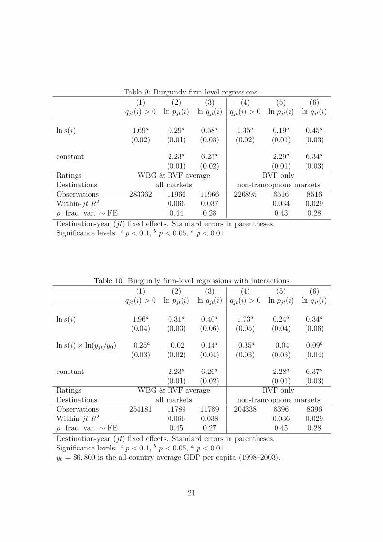
Table 9: Burgundy firm-level regressions


ln s(i) 1.69a 0.29a 0.58a 1.35a 0.19a 0.45a

(0.02) (0.01) (0.03) (0.02) (0.01) (0.03)

constant 2.23a 6.23a 2.29a 6.34a


Destination-year (jt) fixed effects. Standard errors in parentheses.Significance levels: c p < 0.1, b p < 0.05, a p < 0.01

Table 10: Burgundy firm-level regressions with interactions


ln s(i) 1.96a 0.31a 0.40a 1.73a 0.24a 0.34a

(0.04) (0.03) (0.06) (0.05) (0.04) (0.06)

ln s(i)× ln(yjt/y0) -0.25a -0.02 0.14a -0.35a -0.04 0.09b

(0.03) (0.02) (0.04) (0.03) (0.03) (0.04)

constant 2.23a 6.26a 2.28a 6.37a


Destination-year (jt) fixed effects. Standard errors in parentheses.Significance levels: c p < 0.1, b p < 0.05, a p < 0.01y0 = $6, 800 is the all-country average GDP per capita (1998–2003).

21

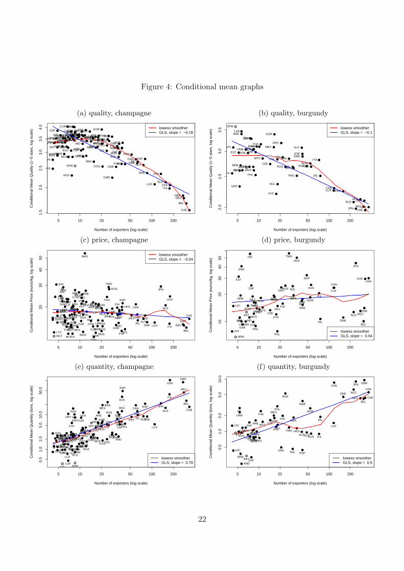
Figure 4: Conditional mean graphs

(a) quality, champagne (b) quality, burgundy

●

●

●

●●

●

●

●

●

● ●●●

●

●

●

●

●

●

●

●

●

●

●●

●●

●

●

●

●●

●

●

●

●

●

●

●

●

●●

●

●

●

●●

●

●

●●

●

●

●

●

●

●

●

●

●

●●

●

●

●●

●

●

●

●

●

●

●

●

●

●

●

●

●●

●

●

●

●

●

●

●

●

●

●

●

●

●

●

●

●

●

●●

●

●

●

●●

●

5 10 20 50 100 200

1.5

2.0

2.5

3.0

3.5

4.0

Number of exporters (log scale)

Con

ditio

nal M

ean

Qua

lity

(1−

5 st

ars,

log

scal

e)

●

●

●

●

●●

AGO

AIA

AND

ANTARE

ARGATG

AUS

AUT

BEL

BEN

BFABHRBHSBMU

BRA

BRB

CAF

CAN

CHE

CHL

CHN

CIV

CMR

COG

COLCRI

CYM

CYPCZE

DEU

DJI

DNK

DOMDZA

EGY

ESP

EST

FIN

GAB

GBR

GHA

GIB

GINGRC

HKG

HRV

HTI

HUNIDN

IND

IRL

ISLISR

ITA

JAM

JOR

JPN

KEN

KHM

KOR

LBN

LCA

LKALTU

LUX

LVA

MARMDG

MDV

MEX

MLI

MLT

MUS

MYS

NCL

NGA

NLD

NOR

NZL

PAN

PERPHL

POL

PRT

PYF

QAT

ROM

RUS

SEN

SGP

SPM

SVNSWE

SYC

SYR

TGO

THA

TTO

TUNTUR

TWNUKRURY

USA

VEN

VGBVNMVUTWLF

ZAF

lowess smootherGLS, slope = −0.18 ●

●

●

●

●

●●

●●

●

●

●

●

●

●

●

● ●●

●

●

●

●

●

●

●

●

●

●

●

●

●

●

●

●●

●

●

●

●

●

●

●

●

●

●

● ●

●

●

●

●

●

●

●

5 10 20 50 100 2002.

02.

53.

03.

5


Con

ditio

nal M

ean

Qua

lity

(1−

5 st

ars,

log

scal

e)

●

●

AND

ANT

ARE

AUS

AUT

BEL

BHSBMU

BRABRB

CAN

CHE

CHN

CIV

CZE

DEU

DNK

DOM ESPEST

FIN

GAB

GBR

GRC

HKG

HTI

IND

IRL

ISL

ISR

ITA

JPN

KOR

LUX

LVA

MEXMLT

MUS

MYS

NCL

NLD

NORNZL

PHL

POL

PRT

PYF

RUS SGP

SPM

SWE

THA

TWN

UKR

USA

VNM

ZAF

lowess smootherGLS, slope = −0.1

(c) price, champagne (d) price, burgundy

●

●

●

●

●

●

●

●●●

●

●

●

●

●

●

●

●

●

●

●●

●

●

●

●

● ●

●

●

●

●

●

●

● ●

● ●

●

●

●

●

●●

●

●

●

●

●

●●

●

●

●

●

●

●

●

●

●

●

●

●

●

●●

●

●

●

●

●

●

●

●

●

●

●

●

● ●

●●

●

●

●

●

●

●

●

●

●

●

●

●

●

●

●

●●

●●

●

●

●

●

5 10 20 50 100 200

2030

4050


Con

ditio

nal M

ean

Pric

e (e

uros

/kg,

log

scal

e)

●

●

●

●

●

●

AGO

AIA

AND

ANT AREARG

ATG

AUS

AUT

BELBENBFA

BHR

BHS

BMU

BRA

BRB

CAF

CAN

CHECHL

CHN

CIVCMR

COG

COL

CRI CYM

CYP

CZE

DEU

DJI

DNK

DOM

DZA

EGY

ESP

EST

FIN

GAB

GBRGHA

GIB

GIN

GRC

HKGHRV

HTI

HUN

IDN

IND

IRL

ISLISR

ITA

JAM

JOR

JPN

KEN

KHM

KOR

LBN

LCA

LKA

LTU

LUX

LVA

MARMDG

MDV

MEX

MLI

MLT

MUS

MYS

NCL

NGANLD

NORNZL

PAN

PER PHL

POLPRT

PYF

QAT

ROM

RUS

SEN

SGP

SPM

SVNSWE

SYC

SYR

TGO

THA

TTO

TUN

TUR

TWN

UKR

URYUSA

VEN

VGB

VNM

VUT

WLF

ZAF

lowess smootherGLS, slope = −0.04

●

●

●

●

●

●

●

●●

●

●

●

●

● ●

●

●

●

●

●

●

●

●

●

●

●●

●

●

●

●

●

●

●

●●

●

●●

●

●

●

●

●

●

●

●

●

●

●

●

●

●

●

●

5 10 20 50 100 200

1020

3040

50


Con

ditio

nal M

ean

Pric

e (e

uros

/kg,

log

scal

e)

●

●

AND

ANT

ARE

AUS

AUT

BEL

BHS

BMU

BRABRB

CAN

CHE

CHN

CIV

CZE DEU

DNK

DOM

ESP

EST

FIN

GAB

GBR

GRC

HKG

HTI

IND IRLISL

ISR

ITA

JPN

KOR

LUX

LVA

MEXMLT

MUS

MYS NCL

NLD

NOR

NZL

PHL

POL

PRT

PYF

RUS

SGP

SPM

SWE

THA

TWN

UKR

USA

VNM

ZAF

lowess smootherGLS, slope = 0.04

(e) quantity, champagne (f) quantity, burgundy

●

●

●

●

●

●

●

●

●

●

●

●●

●

●

●

●●

● ●

●

●

●

●

●

●

●

●

●

●

●

●

●

●

●

●

●

●

●

●

●

●

●

●

●

●

●

●

●

●

●

●

●

●

●

●

●

●●

●

●

●

●

●

●

●

●

●

●

●

●

● ●

●

●

●

●

●

●

●

●

●

●

●

●

●

●

●

●

●

●

●

●

●

●

●

●

●

●

●

●

●

●●

●

5 10 20 50 100 200

0.5

1.0

2.0

5.0

10.0

50.0


Con

ditio

nal M

ean

Qua

ntity

(to

ns, l

og s

cale

)

●

●

●

●

●

●AGO

AIA

AND

ANT

ARE

ARG

ATG

AUS

AUT

BEL

BEN

BFA

BHRBHS

BMU

BRA

BRB

CAF

CAN CHE

CHL CHN

CIV

CMR

COG

COL

CRI CYM

CYP

CZE

DEU

DJI

DNK

DOM

DZAEGY

ESP

EST

FIN

GAB

GBR

GHA

GIBGIN

GRC

HKG

HRVHTI

HUNIDN

IND

IRL

ISL

ISR

ITA

JAM

JOR

JPN

KEN

KHM

KOR

LBN

LCA

LKALTU

LUX

LVA

MAR

MDG

MDV

MEX

MLI

MLT

MUSMYS NCL

NGA

NLD

NOR

NZLPAN

PER

PHL

POL

PRT

PYF

QAT

ROM

RUS

SEN

SGP

SPM

SVN

SWE

SYC

SYR

TGO

THA

TTO

TUN

TUR TWN

UKR

URY

USA

VEN

VGB

VNMVUT

WLF

ZAF

lowess smootherGLS, slope = 0.78 ●

●

●●

●

●

●

●

●

●

●

●

●

●

●●

●

●

●

●

●

●

●

●

●

●

●

●

●●

●

●

●

●

●

●●

●

●

●

●

●

●

●

●

●

●

●

●

●

●

●

●

●

●

5 10 20 50 100 200

0.5

1.0

2.0

5.0

10.0


Con

ditio

nal M

ean

Qua

ntity

(to

ns, l

og s

cale

)

●

●

AND

ANT

ARE

AUSAUT

BEL

BHS

BMU

BRA

BRB

CAN

CHE

CHN

CIVCZE

DEU

DNK

DOM

ESP

EST

FIN

GAB

GBR

GRC

HKG

HTI

IND

IRL

ISL

ISRITA

JPN

KOR

LUX

LVA

MEX

MLTMUS

MYSNCL

NLD

NOR

NZL

PHL

POL

PRT

PYF

RUS

SGPSPM

SWE

THA

TWN

UKR

USA

VNM

ZAFlowess smootherGLS, slope = 0.5

22

models predict equal absolute slopes of opposite signs for the mean price and quantityfigures. The quality sorting model alone predicts the negative average quality-popularityrelationship, negative price-popularity relationship, and positive quantity-popularity re-lationship.

The six scatterplots shown as panels (a)–(f) of Figure 4 mainly support the qual-ity supporting predictions. Average quality and popularity exhibit a strong negativerelationships in panels (a) and (b)—once popularity is sufficiently high. Although therelationship is not globally linear, this may be due to small-sample issues for the lesspopular markets. On the other hand, average quantity and popularity have a strongpositive relationship in panel (e) for champagne and a noisier, but still clearly positiverelationship for red burgundy in panel (f). The mean price panels (c) and (d) are dis-appointing. The slope for red burgundy is close to zero and that for champagne is onlymildly negative. Some very popular markets like Japan (JPN) have high prices that runcounter to the model.

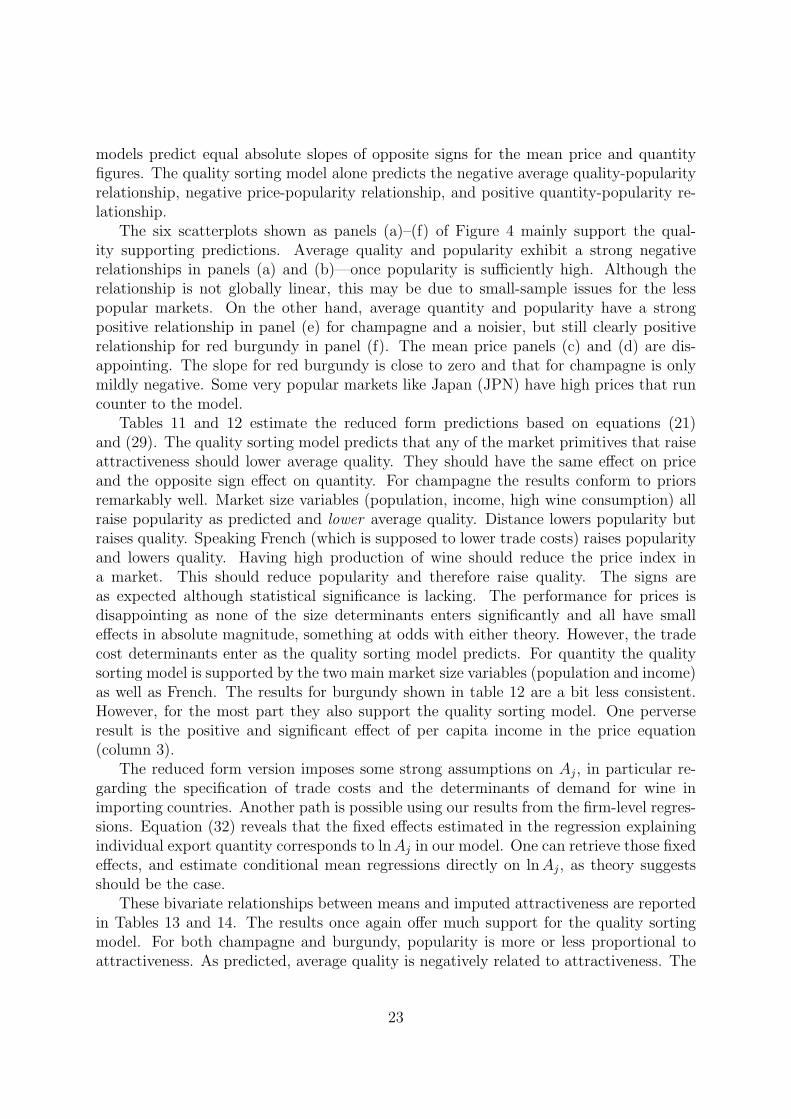
Tables 11 and 12 estimate the reduced form predictions based on equations (21)and (29). The quality sorting model predicts that any of the market primitives that raiseattractiveness should lower average quality. They should have the same effect on priceand the opposite sign effect on quantity. For champagne the results conform to priorsremarkably well. Market size variables (population, income, high wine consumption) allraise popularity as predicted and lower average quality. Distance lowers popularity butraises quality. Speaking French (which is supposed to lower trade costs) raises popularityand lowers quality. Having high production of wine should reduce the price index ina market. This should reduce popularity and therefore raise quality. The signs areas expected although statistical significance is lacking. The performance for prices isdisappointing as none of the size determinants enters significantly and all have smalleffects in absolute magnitude, something at odds with either theory. However, the tradecost determinants enter as the quality sorting model predicts. For quantity the qualitysorting model is supported by the two main market size variables (population and income)as well as French. The results for burgundy shown in table 12 are a bit less consistent.However, for the most part they also support the quality sorting model. One perverseresult is the positive and significant effect of per capita income in the price equation(column 3).

The reduced form version imposes some strong assumptions on Aj, in particular re-garding the specification of trade costs and the determinants of demand for wine inimporting countries. Another path is possible using our results from the firm-level regres-sions. Equation (32) reveals that the fixed effects estimated in the regression explainingindividual export quantity corresponds to ln Aj in our model. One can retrieve those fixedeffects, and estimate conditional mean regressions directly on ln Aj, as theory suggestsshould be the case.

These bivariate relationships between means and imputed attractiveness are reportedin Tables 13 and 14. The results once again offer much support for the quality sortingmodel. For both champagne and burgundy, popularity is more or less proportional toattractiveness. As predicted, average quality is negatively related to attractiveness. The

23

Table 11: Champagne, proxies for Aj

(1) (2) (3) (4)ln Njt ln E [s(i)] ln E [pjt(i)] ln E [qjt(i)]

ln popn. (Mjt) 0.40a -0.07a 0.01 0.37a

(0.05) (0.01) (0.01) (0.06)

ln inc. p.c. (yjt) 0.76a -0.05a 0.02 0.69a

(0.06) (0.01) (0.02) (0.06)

ln cons p.c (µjt) 0.07 -0.04a 0.00 0.03(0.05) (0.01) (0.01) (0.05)

ln prodn (↘ Pjt) -0.04 0.01c -0.00 0.01(0.03) (0.01) (0.01) (0.03)

ln distance (↗ τj) -0.03 0.07a 0.09a 0.10(0.08) (0.02) (0.03) (0.08)

French (↘ τj) 1.53a -0.22a -0.18a 0.61a

(0.18) (0.05) (0.05) (0.14)

constant -4.97a 1.17a 1.96a 0.67(0.93) (0.26) (0.32) (0.90)

Observations 168 160 168 168R2 0.654 0.529 0.212 0.741

GLS, weightj =√

Nj, Standard errors in parenthesesSignificance levels: c p < 0.1, b p < 0.05, a p < 0.01

24

Table 12: Burgundy, proxies for Aj


ln popn. (Mjt) 0.56a -0.05a -0.02 0.39a

(0.07) (0.01) (0.03) (0.05)

ln inc. p.c. (yjt) 1.15a -0.03 0.24a 0.49a

(0.07) (0.02) (0.03) (0.06)

ln cons p.c (µjt) 0.03 -0.02 -0.08b -0.01(0.07) (0.01) (0.03) (0.05)

ln prodn (↘ Pjt) -0.10b 0.01b 0.05a -0.10a

(0.04) (0.01) (0.01) (0.02)

ln distance (↗ τj) 0.01 0.00 0.19a -0.12c

(0.13) (0.02) (0.05) (0.07)

French (↘ τj) 1.32a -0.18a 0.10 0.59a

(0.22) (0.04) (0.12) (0.18)

Constant -9.42a 1.36a -0.64 3.21a

(1.36) (0.31) (0.54) (0.98)Observations 148 112 148 148R2 0.688 0.235 0.451 0.639

GLS, weightj =√


Table 13: Champagne, FE estimate for Aj


ln Ajt 0.97a -0.17a -0.07b 1.18a

(0.09) (0.02) (0.03) (0.04)

Constant 3.02a 0.94a 2.86a 9.18a

(0.15) (0.03) (0.03) (0.06)Observations 176 176 176 176R2 0.432 0.470 0.072 0.808

GLS, weightj =√


25

Table 14: Burgundy, FE estimate for Aj


ln Ajt 0.89a -0.12a -0.04 1.20a

(0.20) (0.02) (0.10) (0.07)

Constant 2.16a 0.87a 2.83a 7.87a

(0.25) (0.02) (0.09) (0.08)Observations 124 124 124 124R2 0.186 0.201 0.003 0.723

GLS, weightj =√


sign on the price effect is supportive of quality sorting but it is only statistically significantfor champagne. Finally the quantity relationships are strongly significant. Indeed theresult is too strong to be consistent with the theory’s prediction that the price andquantity effects be equal in absolute value. The asymmetry in magnitudes we find is alsoat odds with the efficiency sorting model. Taken together with the previous results, itseems to us that the prices are highly noisy and appear to be driven by forces outside thebasic models. Noise in unit values is to be expected but perhaps greater predictive powerwould be possible in a model with some pricing to market. The Dixit-Stiglitz-Krugmanprediction of destination-invariant FOB prices seems hard to square with the results.

6 Conclusion

We have illustrated the importance of quality for trade by examining an industry inwhich quality can be measured (albeit imperfectly). Heterogeneous firms theory impliesa threshold quality for market entry. The result is quality sorting: good firms are betterable to serve difficult markets. We show firms with higher measured quality are more likelyto export, export more, and charge higher prices. Champagne and (to a lesser extent)red burgundy exhibit quality sorting using direct measures. Quantities also respond tomarket attractiveness with the predicted sign. Firm-level prices exhibit much destinationlevel variation that is not predicted by the model. Average prices do not exhibit qualitysorting.

7 References

Baldwin, R. and J. Harrigan. 2007. “Zeros, Quality and Space: Trade Theory andTrade Evidence”, NBER Working Paper No. 13214.

Bernard, A., B. Jensen, S. Redding and P. Schott, 2007, “Firms in International Trade”Journal of Economic Perspectives.

26

Bernard, Andrew B., Jonathan Eaton, J. Bradford Jensen, and Samuel S. Kortum,(2003) “Plants and Productivity in International Trade”, American Economic Re-view, 93(4), 1268–1290.

Chaney, T. 2007. “ Distorted Gravity: the Intensive and Extensive Margins of Interna-tional Trade”, mimeo University of Chicago.

Eaton J., S. Kortum and F. Kramarz, 2004, “Dissecting Trade: Firms, Industries, andExport Destinations”, American Economic Review, Papers and Proceedings, 93:150–154.

Eaton, Jonathan, Samuel Kortum and Francis Kramarz (2006), “An Anatomy of In-ternational Trade: Evidence from French Firms”, University of Minnesota, mimeo-graph.

Hallak, J-C. 2006. “Product Quality and the Direction of Trade,” Journal of Interna-tional Economics 68(1): 238–265.

Helpman, Melitz and Rubinstein, 2007, “Estimating Trade Flows: Trading Partners andTrading Volumes”, mimeo Harvard University.

Hummels, D. and P. Klenow, 2005, “The Variety and Quality of a Nation’s Exports”,American Economic Review, 95, 704-723.

Lawless, M. and K. Whelan, 2007, “A Note on Trade Costs and Distance”, mimeoCentral Bank of Ireland.

Melitz M., 2003, “The Impact of Trade on Intra-Industry Reallocations and AggregateIn- dustry Productivity”, Econometrica, 71(6): 1695-1725.

Melitz, M. and G. Ottaviano, 2007, “Market Size, Trade, and Productivity,”, Review ofEconomic Studies, forthcoming.

Steinberger, Mike, 2005, “American Sparkling Wines: Are they ever as good as cham-pagne?” Slate, Posted at http://www.slate.com/id/2132509/ on Friday, Dec. 30,2005.

27

http://www.slate.com/id/2132509/

A Mean quality: other distributions

We can calculate expected quality with exponential and uniform draws for s. For G(s) =1− exp(−κs) we have

E[s | s > s] = s + 1/κ. (34)

Substituting Nj/Nx in place of s using the inverse CDF, we obtain

E[s | s > s] =ln Nx − ln Nj

κ. (35)

For G(s) = (s− s)/(s− s), we have

E[s | s > s] = (s + s)/2 (36)

Substituting Nj/Nx in place of s using the inverse CDF, we obtain

E[s | s > s] = s− (s− s)Nj

2Nx

. (37)

Thus we see truncated average quality can take various functional forms with respect toNj. However, the general result is that average quality declines with Nj, and thus with inattractiveness of the market(Aj). The effect is stronger when there is greater dispersionin the quality draws: i.e. high s− s or low κ.

28

quality sorting and trade: firm-level evidence for french …ies/fall07/mayerpaper.pdf · quality...

Documents