Summary of Research Activities conducted during the 2012 Summer Semester

Quality, Reliability and Maintenance Laboratory

Research Student: Larkin Liu

Supervisor: Prof Villiam Makis

Department of Mechanical and Industrial Engineering, University of Toronto, 5 King’s

College Road, Toronto, ON, Canada M5S 3G8

Table of Contents:

Acknowledgement

Section A)

Early Gearbox Fault Detection via Auto-Regressive Models in the Time Domain constructed from Vibrational Data & Abstract

1) Introduction

2) Gearbox and Sensor Data:

3) Data Collection

4) Determining TSA intervals using peak-to-peak algorithm

5) Time Synchronous Averaging (TSA)

6) Determining Root Mean Square

7) Order selection and construction of AR Model

8) Obtain Residuals, and set up 3 sigma bounds

9) Conclusion

Section B)

Summary of Miscellaneous Research Contributions for 2012 Summer Semester

B I)

Monitoring the Behavior of Individual Gear Teeth via Residual Data constructed

from Varying-Load Using Vector Auto-Regressive Model of Vibration Data

1) Experimental Overview

2) Monitoring the Behavior of Individual Gear Teeth

2 a) Root Mean Square Method:

2 b) Examining Kurtosis & Skew:

B II) Fourier Analysis to Identify Meshing Frequencies & Harmonics

References

Appendix

Acknowledgement:

Researcher: Larkin Liu

Supervisor: Prof. Villiam Makis

Department of Mechanical and Industrial Engineering, University of Toronto, 5 King’s College Road,

Toronto, ON, Canada M5S 3G8

The content of this report outlines my various contributions to the research activities at

the Quality, Reliability and Maintenance Laboratory at the University of Toronto, from

the duration of June 1st 2012 to August 31st 2012 under the Summer Undergraduate

Research Fellowship provided by the Mechanical and Industrial Engineering

Department of the University of Toronto.

Section A) Early Gearbox Fault Detection via Auto-Regressive Models in the Time Domain constructed from Vibrational Data

Abstract

Vibration-based testing and diagnostic techniques have been widely applied to detect

and prevent the degradation and deterioration of continuously functioning gearboxes.

The typical set up of this technique involves the collection of vibration signal data over

discrete time periods obtained from an array of sensors mounted onto the shell of the

gearbox. During this time frame, the gearbox is subjected to load conditions exceeding

the load-bearing capacities of the machine.

The vibration data collected is used to create an early fault detection scheme for the

machine. In order to process this data, one must first identify the correct meshing

frequency pertaining to the rotating gears. After that, the technique of time-

synchronous-averaging is used to reduce noise and produce a cleaner signal.

Once the signal is processed, an auto-regressive model is constructed from the data

collected from the healthy state. Subtracting the AR model prediction values from the

healthy state observations, we obtain residual values of the vibration signal. A standard

3-sigma control chart based on the residual data in the healthy state is set up and used

to monitor the behavior of the machine leading to early detection of failure.

The result of this research is beneficial in many industries including companies which

operate machines with a critical function that must comply to a guaranteed runtime

prior to failure. Such industries include, aerospace, manufacturing and military.

1) Introduction Vibration signal collection is a condition monitoring method that has attracted

increasing industry interest in recent years. Due to the widespread application of gears

in industrial practice (e.g. automotive, helicopters, aerospace etc.), if interpreted

correctly gearbox vibration data can be applied as a condition indicator of the moving

part of interest, in our case a specific gear in the transmission set up.

In this research, the load applied to the machinery remains constant, thereby

simplifying the procedure. It is worthy to note that in real production environments the

applied loads often vary in time. Therefore the application of this research will only

assist in automated machines that experience approximately constant load conditions

for prolonged periods of time.

Conventional vibrational monitoring techniques, such as this, are based on the

assumption that changes in the vibrational signals are due to the deterioration of the

condition of the gearbox , outlined in Zhan and Makis [2], therefore increasingly erratic

vibrational amplitudes, as well as increased mean value, imply the deterioration of the

machine.

Since the vibrational data is collected from an accelerometer sensor mounted on the

shell of the gearbox, unwanted vibration signals associated with all sorts of transmission

components (such as shafts, bearings etc.) will be recorded. This phenomenon masks

the vibration signal of the gear of interest, and therefore additional signal processing

methods such as time synchronous averaging should be applied to isolate the signal

corresponding to the specific gear.

Using the raw data containing vibrational signals, we use time synchronous averaging to

isolate the target gear. Subsequently, the root mean squared (RMS) value corresponding

to each period of the target gear is calculated to represent the magnitude of vibrational

variation of the rotating gear. Using the RMS values, we create an auto regressive (AR)

model to predict the behavior of the machine over the course of its run time. Observing

the difference between the actual RMS data and AR predicted values, we can use a

control chart to monitor the condition of the gear of interest.

[Figure 1. Flow chart overview of procedure.]

2) Gearbox and Sensor Data:

In this project, the aim was to create an early fault detection scheme for a running

gearbox under constant load conditions. To accomplish this, we used data from

Pennsylvania State University Applied Research Laboratory’s Mechanical Diagnostic

Test Bet (MDTB). In the experiment conducted by MDTB denoted a s Test Run 10, a

single reduction helical gearbox was run until failure. The machine was run at 100% and

then subsequently 200% maximum load.

The aim is to analyze the vibrational data collected from a single sensor, A02, and

analyze the vibration signatures captured by the machine during the runtime,

particularly the time frame where 200% maximum load was applied. During that time

frame the gearbox was running continuously for 93.2 hours until failure.

[Figure 2. Gearbox configuration and run conditions.]

3) Data Collection

During the data retrieval process, raw vibrational signals are directly imported from file

A02 into MATLAB. The vibrational data was collected in 10 second windows at set times

and triggered by accelerometer root mean squared thresholds. We use the threshold as

an indicator for the beginning of each periodic cycle in order to ensure that the data is

synchronous from the beginning of each 10 second window.

The technique of time synchronous averaging can be applied to clean the signal in

accordance to the frequency of the target gear, but first we must identify the time

intervals where synchronous cyclic repetition occurs. Before the collected data can be

interpreted and analyzed, the correct K value, (number of data points pertaining to one

cycle of the target gear) must be obtained in order for the data to be processed correctly.

The [K value] is a property of the mechanical configuration of the gearbox, and is used

to isolate the target gear for failure analysis. To identify the desired [K value] of the

target gear we use the following equation, outlined in Yang and Makis [1].

𝐾 =  𝑓!

𝑓!𝑁!

(1)

where 𝑓! is the sampling frequency of the sensor, 𝑓! is the meshing frequency of the

gears, and 𝑁! is the number of teeth of the target gear.

After obtaining the K value of the gearbox configuration, the collected raw data must be

sectioned into partitions, each the size of the amount of data, prescribed by the meshing

frequency. We begin by assuming that the natural frequency of the target gear should be

embedded in the raw signal. The technique of time synchronous averaging is then

applied to remove the white noise caused by gear shaft imbalance signals, and load

variation signatures etc. [1].

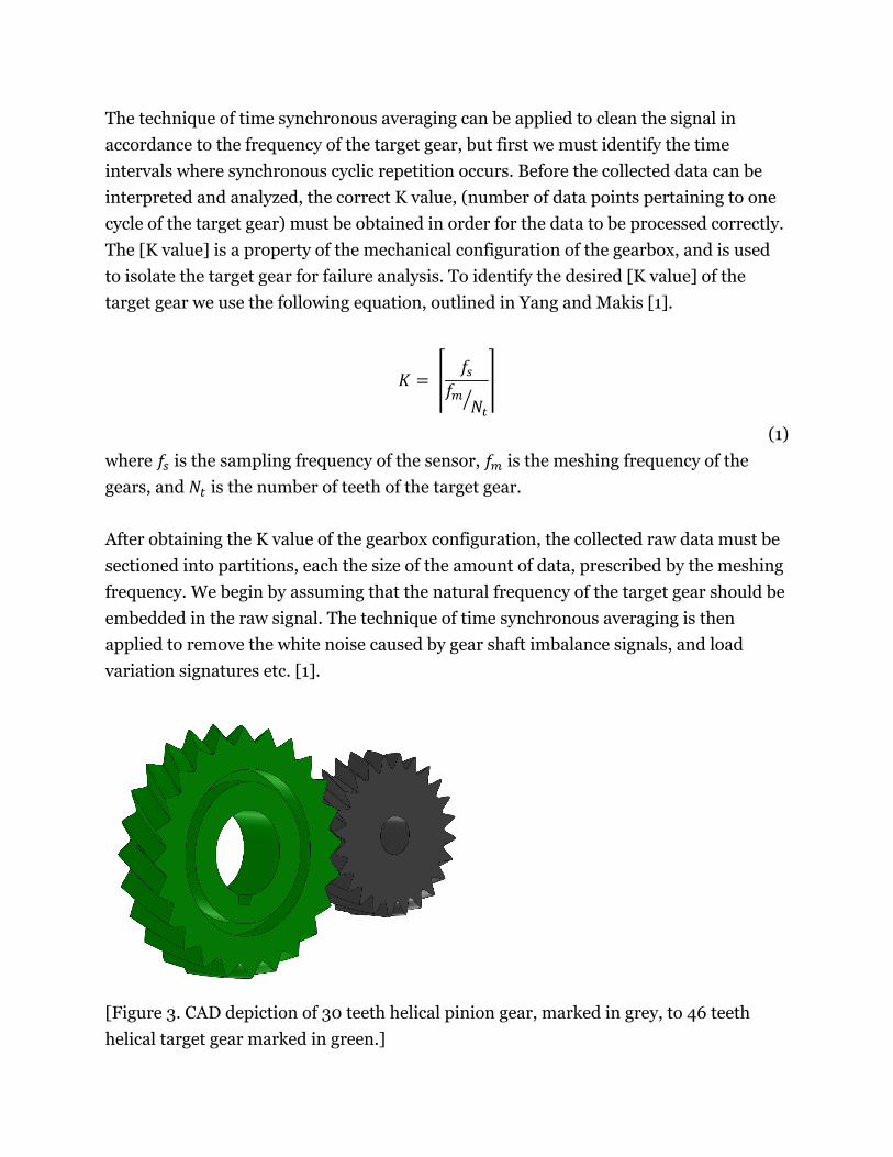
[Figure 3. CAD depiction of 30 teeth helical pinion gear, marked in grey, to 46 teeth

helical target gear marked in green.]

4) Determining TSA intervals using peak-to-peak algorithm

Due to the fact that the gear configuration of the gearbox in in contact with one another,

the varying frequencies excluding the white noise contribution would be considered to

be an effect of the varying harmonics within the gearbox, the dominant frequency being

the meshing frequency of the gear (875 Hz). Therefore, we can expect to observe

periodic behavior within each 10 second window.

The intervals of periodic behavior mark the beginning of repetition within the signal,

where we can subsequently use time synchronous averaging across each repetition to

produce a cleaner signal with reduced noise. However, when performing the peak-to-

peak algorithm independently on each 10 second window data file, the intervals where

peak to peak detection occur are very inconsistent. This is due to the fact that white

noise has a Gaussian distribution of varying amplitudes within the signal.

To produce a cleaner peak-to-peak signal from the 10 second window, with consistent

intervals, we take the averaged signature values over 60 files, and then run a peak to

peak algorithm on it. The results produce a more refined and precise interval locations,

with smaller variability.

In order to find the areas where cyclic repetition occurs, we must first obtain the peak-to

peak intervals within each data file collected. We use a peak-to-peak detection with

MATLAB. The peak-to-peak function “peaks(data)” locates the points where the local

maximum values appear. Using these location points we initiate the time synchronous

averaging algorithm.

5) Time Synchronous Averaging (TSA)

Time synchronous averaging (TSA) involves averaging the periodic data over the range

corresponding to the number of data points representing one cycle of the target gear

[K]. Each interval pertaining to one cycle corresponds to K = 1051 data points, initiated

at the time locations provided by the peak-to-peak algorithm. This ensures that each

packet of time data is synchronous with the next period. Subsequently for each 10

second window, we average periodic intervals corresponding to K data points, at

approximately 190 synchronous starting points, 𝑀!.

𝑀! =   𝑁/𝐾

(2)

Where N is equal to the number of data points corresponding to each 10 second window

(200,000). K is equal to the number of data points pertaining to one cycle of the target

gear (1051).

We begin time synchronous averaging (TSA) by averaging each periodic section of the

data file at the location points provided by the peak to peak algorithm.

TSA Formulation:

𝑽!"#(𝑘) =  1𝑀!

𝑽(𝑘 + 𝑖𝐾)!!!!

!!!

(3)

where, {𝑽!"#(𝑘)} refers to the TSA average of the sequence of 𝑀! points spanning one

period of the averaged sections, {𝑽 𝑘 } is used to denote the discrete time vibration data

within each data file representing a 10 second window, and k denotes the location of

each individual element (k = 1 to k = 1051) within one period of the target gear

frequency.

Once the TSA model is produced, each 10 second window is subsequently summarized

into a collection of K = 1051 data points corresponding to the number of data points

relative to each cycle of the target gear. Each 10 second window consisting of 200,000

data points is compressed into one packet consisting of K = 1051 data points.

Thereafter, each compressed data packed produced by TSA is combined together

chronologically for the purpose of comparison (note that the actual data collected by

each 10 second window pertains to discrete time intervals not necessarily continuous in

nature). Since there are 136 data files pertaining to the gearbox running at 200% load,

there are 136 𝑽!"# packets.

[Figure 4. Raw vibration data collected from sensor A02]

[Figure 5. Vibration data filtered using Time Synchronous Averaging]

6) Determining Root Mean Square

For purposes of simplification, we obtain the Root Mean Square (RMS) value of each

TSA packet. RMS is the measure of varying vibrational quantity indicative of the energy

of the vibration in each target gear cycle.

RMS Formula:

𝑅𝑀𝑆 =   !!

[𝑽!"#(𝑘)]!!

(4)

We see that the when RMS values increases, the process becomes increasingly out of

control.

[Figure 6. Root Mean Square Values with subtracted Mean from first 40 files in the

healthy state]

7) Order selection and construction of AR Model

The next step is to produce an Auto-Regressive model to simulate the future

performance of the gearbox in the healthy state. We use the AR model to model the RMS

values corresponding to the TSA packets to predict the future performance of the

gearbox.

Arbitrarily, we select the first 40 RMS values to be representative of the gearbox in the

healthy state. Also, we create 20 AR models based on lag orders 1 through 20 and

evaluate the Akaike Information Criterion (AIC) of each AR model based on the

respective lags to determine which model is the best.

We select the lag order which produces the lowest AIC value to model the behavior of

the RMS values in the healthy state. In this experiment, the lowest AIC value was

“6.6213” corresponding to the lag order 12. Therefore, an AR model with the lag order 12

was used to produce a healthy state model of the gearbox.

AIC formula:

AIC = 2k – 2ln(L)

(5)

L is the maximum likelihood function for each AR model, and k is the number of

parameters of the model. In order, to obtain the AIC values of each model in MATLAB,

we first use the “ar(data, lag)” function in MATLAB to generate the model parameters.

The “ar” function implements the Yule-Walker equations [7] to determine the

coefficients for the AR model. After, the AR model is fed into the function “aic(model)”,

part of the MATLAB System Identification Toolbox to determine the Akaike Index

Criterion of the model.

[Figure 7. AIC Values for AR models constructed from lag orders 1 to 20, with optimal

lag order of 12 marked in light green.]

Once the optimal lag order is known, we use the AR parameters generated from the

optimal lag order to forecast the behavior of the gearbox running in the healthy state.

[Figure 8. AR model of lag order 12 in green, RMS mean subtracted model in blue, area

to the left of the red dashed line indicates region pertaining to the healthy state of the

machine.]

8) Obtain Residuals, and set up 3 Sigma Bounds

In order to produce a control chart from the collected data, the AR model prediction of

the data generated from MATLAB is subsequently subtracted from the RMS values of

the observed data to obtain the error of the prediction, defined as the residual value. We

stipulate that the first 40 residual values pertain to the gearbox running in healthy state,

which we denote as the training data. And thus, the files from 41 to 136 corresponding to

the gearbox testing data, is utilized to monitor the condition of the gearbox.

Calculating the standard deviation of the residual data in the training phase we obtain

the 3-sigma bounds which are used to monitor the entire run time. Evaluating the

values of the RMS residual data, we can determine whether the process is in control or

not.

[Figure 9. Control Chart Residuals.]

We can see from the residual chart that the process has points falling outside of the

control bounds beginning with the file 'A0200310.010' '09-Jul-1998 15:06:32' [marked

in orange]. This indicates an anomaly in the state of the machine, and thus preventive

maintenance planning should begin to reduce the chance of failure.

From file 'A0200356.010' '09-Jul-1998 15:06:48' and onwards (marked in red), we can

see that the vibrational state of the machine is becoming extremely unstable, as

successive residual points fall outside of the 3 sigma limit. Therefore, preventive

maintenance should be preformed immediately.

9) Conclusion

The transmission fault detection scheme presented in this report was successful in

detecting the time where preventive maintenance should be planned, and also the time

where severe deterioration begins. A conventional TSA algorithm was used to isolate the

signals pertaining to the target gear. RMS values were calculated to represent the

varying quantity of each TSA packet representing a 10 second window. An AR model

was produced from the portion of the gearbox running in the healthy state. From the AR

model, residual values were obtained and used to monitor the condition of the machine

via control chart methods.

The application of this research can have an effective impact not only on preventive

maintenance but also on the quality assurance of machines. Industries which may find

suitable use for control chart methods to assist in fault detection and quality assurance

include military, power generation, automotive, and manufacturing. Of these industries,

there often exist machines which mandate a guaranteed run time before failure, and

thus a scheme to provide scheduled preventive maintenance would be beneficial in

order to reduce the chance of failure during the guaranteed run time.

Future considerations of this research include the utilization of more advanced

statistical models to model the vibrational phenomena. Such models include auto-

regressive moving average (ARMA) or auto-regressive exogenous (ARX) models. Using

these models, it is possible to create a fault detection scheme for machines operating

under varied loads [1].

Furthermore, instead of providing an AR model based on the RMS values, it is possible

to construct an AR model based on the actual vibration signal, such procedures would

require much greater computing power, and also more efficient algorithms. Also, more

advanced signal processing methods, such as harmonic filtering and Fourier analysis,

could be considered to produce even more refined and cleaner signals corresponding to

the target gear. The aforementioned future improvements could possibly enhance the

accuracy and utility of the fault detection scheme.

Section B) Summary of Miscellaneous Research Contributions for 2012 Summer Semester

B I) Monitoring the Behavior of Individual Gear Teeth via Residual Data

constructed from Varying-Load Using Vector Auto-Regressive Model of Vibration Data 1) Experimental Overview

In the research paper, “Detection of Gearbox Deterioration under Varying-Load Using

Vector Auto-Regressive Model of Vibration Data” [4], the goal was to create a fault

detection scheme for a varying load gearbox, by creating a Vector Autoregressive model

(VAR) model constructed from vibration data. The studied vibration data was obtained

from the Mechanical Diagnostic Test Bed (MDTB) built by Pennsylvania State

University Applied Research Laboratory Condition-Based Maintenance Department.

The MDTB gearbox contained a 70-tooth driven helical gear and a 21-tooth pinion gear,

driven at a set input speed using a 30 Hp, 1750 rpm drive motor, with the torque applied

by a 75 HP, 1750 rpm absorption motor [5].

2) Monitoring the Behavior of Individual Gear Teeth

The objective of this procedure was to capture the irregularities occurring during the run

time of the gear corresponding to each gear teeth. In the aforementioned experiment

conducted by MDTB, seven gear teeth were found to have deteriorated severely.

Therefore, if each gear teeth was isolated and monitored, we would expect data

pertaining to these seven gear teeth to show signs of deterioration.

During the entire run time, 93 vibrational data files spanning to 10 second time intervals

were captured. Each data file was time-synchronous averaged into K = 2285 data points,

corresponding to the number of data points representing one revolution of the target

gear [1].

𝐾 =  𝑓!

𝑓!𝑁!

(1)

We theorized that if we were to monitor the residual data obtained by subtracting the

VAR model from the actual vibration, we could monitor condition of each gear teeth. To

do this, we applied the use of 3 indicators, root mean square, kurtosis, and skew.

For all 93 “10 second windows”, we isolated it into data segments pertaining to each

gear teeth,

𝑘! =   𝐾/𝑁! = 2285/70 = 32

(6)

Where kt represents the number of data points representing each gear tooth, K is the

number of data points representing one revolution of the gear, Nt represents the number

of teeth. Therefore, each 32 residual data points represents one gear teeth, allowing us

to compute the RMS, Kurtosis, and Skew from the residual data of each gear teeth.

2 a) Root Mean Square Method:

The RMS captures the varying quantity of vibration of each gear tooth constructed from

the residual data. We stipulate that the increase in varying quantity, conveyed by the

increase in RMS value, indicates failure of the gear teeth.

[Figure 10. Sample RMS Values for Gear Teeth #16 ]

We found that while obtaining the RMS for each gear tooth, files pertaining to all gear

teeth on the target gear experienced increasing RMS values, as oppose to specifically the

seven gear teeth where severe deterioration were found after physical inspection. This

indicates that the deterioration of one gear teeth influences vibrational anomalies within

the entire mechanical system, thus we were unable to isolate and monitor each gear

teeth in particular using the RMS method.

2 b) Examining Kurtosis & Skew:

We assume that the residual data should be normally distributed for each gear tooth

operating in the healthy state. The kurtosis of the distribution captures the peaked-ness

of the distribution of residual data respective to the normal distribution. If the kurtosis

value increase in positive value, the distribution becomes more peaked. On the contrary,

if the kurtosis value becomes increasingly negative, the distribution becomes more “bell

shaped". [6]

The skewness measures the symmetry of the residual data distribution. An increasing

skew value away from zero indicates increasing dissymmetry, conveying that data is

distributed more to either the left or right. Whereas a skew value of zero indicates

perfect symmetry.

[Figure 11, Average Kurtosis values for each gear teeth 1 - 70 ]

We use these indicators, skewness and kurtosis, to measure the normality of data over

the run time. When the data becomes less adherent to the normal distribution we take

this as an indicator of deterioration.

After computing the kurtosis of the residual data pertaining to each gear tooth, we took

the average kurtosis of each gear tooth throughout time. We found that the average

kurtosis values remained below zero for all data files pertaining to each gear tooth,

indicating an imperfect normality distribution for all gear teeth pertaining to the target.

Moreover, the average skew of the residual data pertaining to each gear teeth on the

target gear all oscillated around the zero mark, the skew value was not indicative of

failure on any data file pertaining to specific gear teeth.

[Figure 12. Average skew values of gear teeth 1-70]

Overall, the objective to identify and monitor the specific gear teeth via RMS, kurtosis,

and skewness gave no conclusive results.

B II) Fourier Analysis to Identify Meshing Frequencies & Harmonics

One signal processing approach was to filter out raw vibration data using Fourier

transform to transform the data from the time domain to the frequency domain. This

allows us to identify the dominant and harmonic frequencies contained in the signal. To

accomplish we implemented a Fast Fourier Transform, which is an algorithm to

approximate the Discrete Fourier Transform [3].

The dominant frequency pertaining to the main meshing frequency was found to be

613 Hz, 3.065% of the meshing frequency ( fs ) of 20,000 Hz. The harmonic frequencies

resonating from that frequency was found to be, 1226 Hz,1839 Hz, 2452 Hz, all integer

multiples of the meshing frequency.

[Figure 13. Fast Fourier Transform of raw vibration signals in the frequency domain. X

axis indicates the percentage of the meshing frequency of 20,000 Hz.]

Subsequently, one could implement a high/low pass filter to filter out the signal. This

step was not carried through, however, we were successful in identifying the various

frequencies contained within the signal. The most dominant frequency contained within

the signal was the theoretical meshing frequency of 613 Hz.

References

[1] Yang, Ming, and Viliam Makis. "ARX Model-based Gearbox Fault Detection and Localization

under Varying Load Conditions." Journal of Sound and Vibration 329.24 (2010): 5209-221.

Print.

[2] Zhan, Yimin, and Viliam Makis. "A Robust Diagnostic Model for Gearboxes Subject to Vibration

Monitoring." Journal of Sound and Vibration 290.3-5 (2006): 928-55. Print.

[3] FFT Tutorial. Jesse's Homepage. University of Rhode Island, n.d. Web.

<http://www.ele.uri.edu/~hansenj/>.

[4] Lin, Chen, and Villiam Makis. "Detection of Varying-Load Gearbox Vibration by Using Vector

Autoregressive Model." Proceedings of the International Conference on Mechanical

Engineering and Mechatronics (2012): n. pag. Print.

[5] "Applied Research Laboratory - Serving America's Defense, Industry, and Education." Applied

Research Laboratory. N.p., n.d. Web. 28 Aug. 2012. <http://www.arl.psu.edu/>.

[6] DeCarlo, Lawrence T. "On the Meaning and Use of Kurtosis." Psychological Methods 2.3 (1997):

292-307. Print.

[7] Chen, Weitian, Brian D.O. Anderson, Manfred Deistler, and Alexander Filler. "Solutions of Yule-

Walker Equations for Singular AR Processes." Journal of Time Series Analysis 32.5 (2011): 531-

38. Print.

Appendix

Estimating AR parameters using Yule-Walker equations via MATLAB

The Auto-Regressive (AR) model prediction model which takes into consideration

previous observations corresponding to the lag order.

𝑌! = 𝑐 +   𝜑!𝑌!!!

!

!!!

+  𝜀!

(i)

Where, 𝑌! is the observation at time t, 𝑌!!! is the observation at lag t-i , 𝜑! is the AR

parameter for the lag order i, p is the lag order of the AR model, c is a constant

representing the mean value of the observation, (in our case 0) since we subtracted the

healthy state mean out of the RMS values, and 𝜀! is the noise at time t.

Therefore,

𝑌! = 𝑌! −  𝜀!

where 𝑌! is the AR prediction at time t.

The parameters used to create the AR model based on the lag order 12 were estimated

using the Yule Walker algorithm [7] in MATLAB using the function “aryule(data)”, part

of the system identification toolbox.

Estimating the AR parameters based on the RMS mean subtracted values we found the

AR parameters at lags 1 through 12, respectively to be

0.1212 -0.0923 -0.0162 0.0861 -0.2123 0.2562 0.1524 0.1723 -0.0388

0.0460 -0.0182 -0.0085