quality of service analysis of internet links with minimal information
TRANSCRIPT

UNIVERSIDAD AUTONOMA DE MADRID
ESCUELA POLITECNICA SUPERIOR
Ph.D. Thesis
Quality of Service Analysis of Internet
Links with Minimal Information
Author:Felipe Mata Marcos
Supervisor:Prof. Javier Aracil Rico
Madrid, 2012


DOCTORAL THESIS: Quality of Service Analysis of InternetLinks with Minimum Information
AUTHOR: Felipe Mata Marcos
SUPERVISOR: Prof. Javier Aracil Rico
The committee for the defense of this doctoral thesis is composed by:
PRESIDENT: Prof. TBA
MEMBERS: Dr. TBA
Dr. TBA
Prof. TBA
SECRETARY: Dr. TBA


To my parents


Summary
Monitoring the Quality of Service (QoS) of Internet links is of paramount
importance for Network Operators and Service Providers (NOSP), and con-
sequently has received great attention from the research community. To
monitor QoS, practitioners leverage on network traffic measurements and,
by means of practical models and statistical techniques, make predictions
and detect outliers that allow the planning of telecommunication networks
and the detection of abnormal behavior, respectively.
However, obtaining detailed measurements from Internet links at current
network speeds is very challenging, mainly because memory accesses’ speeds
have increased at a smaller pace than Internet links’ speeds. Moreover, the
amount of resources required to properly storage detailed network measure-
ments make unfeasible to perform long measurement campaigns. These facts
have motivated the application of different techniques to gather information
from the network, such as collecting subsets of network traffic by applying
sampling techniques in the packet capture process, or just collecting sum-
marized statistics of the number of bytes transferred, such as those used
in Multi Router Traffic Grapher (MRTG), where the maximum and aver-
age transfer speeds are recorded at non-overlapping time intervals of a given
length. These techniques make network traffic monitoring less demanding
and allow performing longer measurement campaigns.
Accordingly, this thesis proposes two methodologies to perform QoS anal-
ysis of Internet links leveraging on summarized statistics of network traffic.
Each methodology relies on a network traffic model, validated using actual
network traffic measurements, on which sound statistical methodologies are
used on attempts of detecting relevant events that either require action from
vii

viii Summary
the network managers or may be related with degradations of the provided
QoS.
The first methodology is designed to detect shifts in users’ behavior, and
consequently the detected events may entail capacity planning decisions. It
builds on modeling the network traffic during a day using a multivariate
fairly Gaussian distribution, from which changes in the parameters are de-
tected at timescales of weeks. The change point instants are detected using
clustering techniques and validated through the application of the Multivari-
ate Behrens-Fisher Problem (MBFP). The proposed methodology is applied
to real network measurements obtained from the Spanish academic network
RedIRIS, showing satisfactory performance and entailing large Operational
Expenditures (OPEX) reduction to NOSP in the management process of
large-scale networks.
The second methodology performs anomaly detection through trend re-
moval of network traffic measurements. It is tailored for Voice over IP (VoIP)
traffic data, which is one of the most popular services provided through In-
ternet nowadays. The methodology takes as input call count measurements
of the VoIP service exhibiting seasonal trends, and outputs stationary resid-
uals, which are used to detect anomalies by means of the application of un-
sophisticated statistical assumptions. Moreover, we propose a measurement
alternative for monitoring VoIP systems. This alternative yields smaller cor-
relations between the obtained measurements when some assumptions are
met, which we showed to be satisfied in actual measurements we analyzed.

Resumen
Monitorizar la Calidad de Servicio (QoS, de sus siglas en ingles) de enlaces
de Internet es de vital importancia para Operadores de Red y Proveedores de
Servicio (NOSP, de sus siglas en ingles), y por tanto ha recibido gran atencion
por parte de la comunidad cientıfica. Para monitorizar la QoS, los expertos
usan medidas del trafico de red y, mediante la aplicacion de modelos practicos
y tecnicas estadısticas, hacen predicciones y detectan valores atıpicos que
permiten el dimensionado de redes de telecomunicaciones y la deteccion de
comportamiento anomalo, respectivamente.
Sin embargo, obtener medidas detalladas de enlaces de Internet a las
velocidades de red actuales es muy exigente, principalmente porque las velo-
cidades de acceso a memorias han crecido a menor ritmo que las velocidades
de los enlaces de Internet. Ademas, la cantidad de recursos requerida para
almacenar apropiadamente medidas de red detalladas hace imposible realizar
largas campanas de medidas. Estos hechos han motivado la aplicacion de
diferentes tecnicas para recolectar informacion de la red, tales como recopilar
subconjuntos del trafico de red mediante la aplicacion de muestreo en el
proceso de captura de paquetes, o simplemente la recopilacion de estadısticos
resumidos del numero de bytes transferidos, como los usados en Multi Router
Traffic Grapher, donde la tasa de transmision maxima y media son recogidas
en intervalos disjuntos de una longitud dada.
Por consiguiente, esta tesis propone dos metodologıas para realizar analisis
de QoS en enlaces de Internet usando estadısticos resumidos del trafico de
red. Cada metodologıa se basa en un modelo del trafico de red, validado
con medidas de trafico de red reales, sobre los cuales tecnicas estadısticas
fiables son aplicadas con el objetivo de detectar eventos relevantes que o bien
ix

x Resumen
requieren actuacion por parte de los gestores de red o quiza esten relacionados
con degradaciones de la QoS provista.
La primera metodologıa esta disenada para detectar variaciones en el
comportamiento de los usuarios, por lo que los eventos detectados pueden
conllevar decisiones de dimensionado de red. Primero modelamos el trafico de
red a lo largo de un dıa usando una distribucion multivariante practicamente
Gaussiana, mediante la cual cambios en sus parametros son detectados en
escalas de tiempo de semanas. Los instantes de cambio se detectan usando
tecnicas de clustering y son validados mediante la aplicacion del Problema
de Behrens-Fisher Multivariante. La metodologıa propuesta se ha aplicado
a medidas reales de trafico de red obtenidas de la red academica espanola
RedIRIS, demostrando un rendimiento satisfactorio y conllevando para los
NOSP grandes reducciones de los gastos operacionales en el proceso de gestion
de redes de gran escala.
La segunda metodologıa realiza deteccion de anomalıas mediante la elimi-
nacion de la tendencia existente en medidas del trafico de red. Esta especıfi-
camente disenada para trafico de Voz sobre IP (VoIP, de sus siglas en ingles),
que es uno de los servicios mas populares ofrecidos a traves de Internet hoy en
dıa. La metodologıa utiliza medidas de la cantidad de llamadas en el servicio
VoIP que exhiben tendencias periodicas, y las transforma en residuos esta-
cionarios que son usados para detectar anomalıas mediante la aplicacion de
asunciones estadısticas poco sofisticadas. Ademas, tambien proponemos una
forma alternativa de monitorizar sistemas de VoIP. Esta alternativa produce
menores correlaciones entre las medidas obtenidas cuando algunas asunciones
se cumplen, las cuales son satisfechas concretamente en las medidas de trafico
real que hemos analizado.

Acknowledgments
It is difficult to write technical papers clear and concisely (moreover if you
have to write them in a foreign language), but it is more difficult to properly
write an acknowledgment, being fair with all the people that helped you,
either by directly working side by side, or by supporting and understanding
your situation externally. Therefore, I would like to explicitly thank those
people, whose help has mainly impacted my researching career and my whole
life, apologizing to those ones not mentioned. This work is dedicated to all
of them.
Firstly, I would like to thank my family for their support and under-
standing every time, although I have not been able to spend as much time
with them as I desire—however, I expect this situation to change from now
on. Their protection and upbringing have made up the man that I am
nowadays—well, not completely, they are only responsible for those good
things I sometimes do.
Although my friends’ contribution to this work is arguable (sorry dudes,
but you are better for wasting time ;-]!), they also merit to be acknowledged,
because taking the most of the spare time helps me to be productive during
working hours. Maybe since I started the PhD my free time is reduced and
I am not able to see you frequently, but it does not mean our relationship is
worse, it just changed. Nobody could snatch me the memories of the good
moments we have spent together.
A special acknowledgment is dedicated to my supervisor, Javier Aracil,
for his close collaboration and good advise, the fruitfulness of this work and
the forthcoming ones is mainly your duty. Thank you for allowing me to
start my researching career here. In the same way, I would like to thank my
xi

xii Acknowledgments
colleagues from the Networking Research Group: Javier Ramos, Pedro San-
tiago, Jaime Garnica, Vıctor Moreno, David Muelas, Santiago Pina, German
Retamosa, David Madrigal, Jorge Lopez de Vergara, Sergio Lopez, Paco
Gomez, Ivan Gonzalez, Luis de Pedro, Gustavo Sutter, and those that are
no longer here: Vıctor Lopez, Bas Huiszoon, Alfredo Salvador, Jose Alberto
Hernandez, Diego Sanchez, Jaime Fullaondo and Walter Fuertes. A singu-
lar mention is deserved to Jose Luis Garcıa, from whom I learned so much.
Thank you for all this time at the laboratory and all the good moments we
have shared. This also definitely includes my other colleagues from the labo-
ratory Pedro Gomez, Alvaro Garcıa and Miguel Cubillo. All my work would
not have been possible without the support of the Universidad Autonoma
de Madrid and the Departamento de Tecnologıa Electronica y de las Comu-
nicaciones (former Departamento de Informatica) of the Escuela Politecnica
Superior.
In addition, I would also like to express my gratitude to RedIRIS for
providing us with traffic measurements that have been fundamental to this
thesis, to the Spanish Ministry of Education and Science that has funded this
research under the F.P.U. fellowship program, and the COST TMA action
that has helped me to grow as a researcher. Specially related to the TMA
action, I would like show my gratefulness to Raimund Schatz and Michel
Mandjes for hosting me in Wien and Amsterdam, respectively.
My stay in Wien was very constructive. I learned a lot in the topic of
Quality of Experience, which I think is going to be one of the most fertile
field of research in networking. I would like to thank Peter Fr’ohlich and
Michal Ries for their comprehension and patience with me. This includes all
the members of The Telecommunications Research Center Vienna (FTW),
in particular the Settanni twins.
From my TMA STSM in Amsterdam I retain great memories. Further-
more, it was very productive. This stay helped me to grow up, both as a
researcher and as a person. Moreover, I learned a lot with the discussions with
Michel, and working side by side with Piotrek Zuraniewski, who in addition
helped me a lot to integrate in Universiteit van Amsterdam’s lifestyle and
feel less lonely. This absolutely includes all the staff and other students from

Acknowledgments xiii
the Korteweg-de Vries Institute for Mathematics, specially Ricardo Reis. Al-
though not in person, I also had the chance to work with Marco Mellia during
my STSM at Amsterdam. Furthermore, our achievements would not have
been possible without the VoIP traffic traces that Marco kindly shared with
us. I would like to sincerely express my gratitude to Marco and Telecommu-
nication Network Group of Politecnico di Torino members for allowing me
the use of such data in this thesis.
Last, but for sure not the least, Cristina, I dedicate this work to you.
Your company, support and understanding are invaluable. Thank you for
being by my side, we have to celebrate this! (yes yes, I pay...;-])


Contents
Title Page i
Summary vii
Resumen ix
Acknowledgments xi
Contents xvii
List of Figures xix
List of Tables xxiii
Acronyms xxxii
1 Introduction 1
1.1 Overview and Motivation . . . . . . . . . . . . . . . . . . . . . 1
1.2 Objectives and Hypothesis . . . . . . . . . . . . . . . . . . . . 3
1.3 Thesis Structure . . . . . . . . . . . . . . . . . . . . . . . . . . 4
2 State of the Art 7
2.1 Network Measurements . . . . . . . . . . . . . . . . . . . . . . 7
2.1.1 Packet Captures . . . . . . . . . . . . . . . . . . . . . . 8
2.1.2 NetFlow Records . . . . . . . . . . . . . . . . . . . . . 9
2.1.3 MRTG Records . . . . . . . . . . . . . . . . . . . . . . 11
2.2 Anomaly Detection . . . . . . . . . . . . . . . . . . . . . . . . 12
xv

xvi Contents
2.2.1 Introduction . . . . . . . . . . . . . . . . . . . . . . . . 13
2.2.2 Anomaly Intrusion Detection Taxonomy . . . . . . . . 15
2.2.3 Anomaly Intrusion Detection Techniques . . . . . . . . 26
2.2.4 Problems of Anomaly Intrusion Detection . . . . . . . 84
2.2.5 Future Trends in Anomaly Intrusion Detection . . . . . 90
2.2.6 Conclusions . . . . . . . . . . . . . . . . . . . . . . . . 91
3 Detection of Traffic Changes in Large-Scale Backbone Net-
works 93
3.1 Introduction . . . . . . . . . . . . . . . . . . . . . . . . . . . . 93
3.2 Measurement Dataset . . . . . . . . . . . . . . . . . . . . . . . 98
3.2.1 Description of the Measurement Dataset . . . . . . . . 98
3.2.2 RedIRIS Daily and Weekly Traffic Patterns . . . . . . 100
3.3 Multivariate Normal Model for Daily
Traffic . . . . . . . . . . . . . . . . . . . . . . . . . . . . . . . 101
3.3.1 Description of the Multivariate Normal Model . . . . . 102
3.3.2 Methodology . . . . . . . . . . . . . . . . . . . . . . . 105
3.3.3 Results of the Model Validation . . . . . . . . . . . . . 107
3.3.4 Discussion of the Results . . . . . . . . . . . . . . . . . 109
3.4 On-line Load Change Detection Algorithm . . . . . . . . . . . 110
3.4.1 Methodology . . . . . . . . . . . . . . . . . . . . . . . 111
3.4.2 Description of the Algorithm . . . . . . . . . . . . . . . 113
3.4.3 Validation of the Algorithm . . . . . . . . . . . . . . . 113
3.5 Change Point Analysis with Real
Network Measurements . . . . . . . . . . . . . . . . . . . . . . 121
3.6 Network Management Based on Relevant Events . . . . . . . . 126
3.7 Summary and Conclusions . . . . . . . . . . . . . . . . . . . . 129
4 Weekly Pattern Timeseries Detrending: The Case of VoIP 131
4.1 Introduction . . . . . . . . . . . . . . . . . . . . . . . . . . . . 132
4.2 Related Work . . . . . . . . . . . . . . . . . . . . . . . . . . . 134
4.3 Measurement Dataset . . . . . . . . . . . . . . . . . . . . . . . 137
4.3.1 Daily and Weekly Patterns . . . . . . . . . . . . . . . . 138

Contents xvii
4.3.2 Call Arrival Process . . . . . . . . . . . . . . . . . . . 138
4.3.3 Call Holding Time Distribution . . . . . . . . . . . . . 140
4.4 Detrending Methodology . . . . . . . . . . . . . . . . . . . . . 142
4.4.1 Methodology Description and Expected Results . . . . 143
4.4.2 Model Performance Results . . . . . . . . . . . . . . . 144
4.5 Measurement Alternative . . . . . . . . . . . . . . . . . . . . . 148
4.5.1 Alternative Proposal . . . . . . . . . . . . . . . . . . . 148
4.5.2 Correlations Study: Dependence on the Service Time
Distribution . . . . . . . . . . . . . . . . . . . . . . . . 150
4.6 Anomaly Detection Algorithm . . . . . . . . . . . . . . . . . . 155
4.6.1 Description of the Algorithm . . . . . . . . . . . . . . . 156
4.6.2 Anomaly Detection in VoIP Data . . . . . . . . . . . . 158
4.7 Summary and Conclusions . . . . . . . . . . . . . . . . . . . . 162
5 Conclusions 163
5.1 Main Contributions . . . . . . . . . . . . . . . . . . . . . . . . 163
5.2 Future Work . . . . . . . . . . . . . . . . . . . . . . . . . . . . 167
Conclusiones 169
References 177
List of Publications 227
A Kolmogorov-Smirnov Test and Lilliefors’ Correction 231
B Behrens-Fisher Problem 233
B.1 Univariate Behrens-Fisher Problem . . . . . . . . . . . . . . . 233
B.2 Multivariate Behrens-Fisher Problem . . . . . . . . . . . . . . 234
C Analysis of Hotelling’s T 2 Statistic 237
D Affine Transformations 241
Index 243


List of Figures
2.1 RedIRIS Points of Presence. . . . . . . . . . . . . . . . . . . . 10
2.2 Sample one-day MRTG monitoring. . . . . . . . . . . . . . . . 11
2.3 General taxonomy of Anomaly-based Intrusion Detection Sys-
tems that is applicable to Misuse-based Intrusion Detection
Systems. . . . . . . . . . . . . . . . . . . . . . . . . . . . . . . 16
2.4 Taxonomy of Anomaly-based Intrusion Detection principles
proposed by Axelsson. . . . . . . . . . . . . . . . . . . . . . . 19
2.5 Detailed taxonomy of Anomaly-based Intrusion Detection prin-
ciples proposed by Verwoerd and Hunt. . . . . . . . . . . . . . 20
2.6 Fine-grained taxonomy of Anomaly-based Intrusion Detection
principles proposed by Patcha and Park. . . . . . . . . . . . . 21
2.7 Fine-grained taxonomy of Anomaly-based Intrusion Detection
principles proposed by Garcıa-Teodoro et al. . . . . . . . . . . 22
2.8 Exhaustive taxonomy of Anomaly-based Intrusion Detection
principles proposed by Chandola et al. . . . . . . . . . . . . . 23
2.9 Taxonomy of computational intelligence systems applied to
Anomaly-based Intrusion Detection proposed byWu and Banzhaf. 24
2.10 Taxonomy proposal of Anomaly-based Intrusion Detection tech-
niques. . . . . . . . . . . . . . . . . . . . . . . . . . . . . . . . 25
3.1 RedIRIS network architecture. . . . . . . . . . . . . . . . . . . 99
3.2 Time Series representation of the utilization of a RedIRIS link
for a whole week. . . . . . . . . . . . . . . . . . . . . . . . . . 101
xix

xx List of Figures
3.3 Time Series representation of the average utilization pattern
of the RedIRIS network and time divisions according to the
multivariate model. . . . . . . . . . . . . . . . . . . . . . . . . 104
3.4 Univariate and multivariate normality test results. . . . . . . . 108
3.5 Work-flow of the on-line algorithm. . . . . . . . . . . . . . . . 114
3.6 False Positives Ratio in datasets with no changes. . . . . . . . 116
3.7 Detected changes in the staggered increments datasets. . . . . 117
3.8 Time Series representation of the change-free regions for the
first 300 samples. . . . . . . . . . . . . . . . . . . . . . . . . . 119
3.9 Zoom to the first four change-free regions of the 1st vector
component with delimitation lines for the theoretical change
points. . . . . . . . . . . . . . . . . . . . . . . . . . . . . . . . 120
3.10 Change points found by the on-line algorithm on the time
interval 10:30-12:00. . . . . . . . . . . . . . . . . . . . . . . . . 124
3.11 Examples of Sample Autocorrelation Function and Sample
Cross-correlation Function functions of the binary time series. 125
3.12 Sample weather map of the RedIRIS network, with some links
needing the network manager attention. . . . . . . . . . . . . 128
4.1 Average weekly pattern of the analyzed dataset. . . . . . . . . 138
4.2 Log-log plots of the data and best fitting models. . . . . . . . . 142
4.3 Data samples for the week under study and estimated pattern
based on previous weeks data samples. . . . . . . . . . . . . . 145
4.4 Residuals obtained after standardization with the estimated
pattern. . . . . . . . . . . . . . . . . . . . . . . . . . . . . . . 145
4.5 Gaussian Quantile-Quantile plots of the residuals. . . . . . . . 146
4.6 Autocorrelations of the residuals with nights included and re-
moved. . . . . . . . . . . . . . . . . . . . . . . . . . . . . . . . 147
4.7 Contour plots showing the isopleths of comparing the correla-
tions computed using both measurement alternatives (Corr(N0, Nt)−Corr(H0, Ht)) when the service time distribution is assumed
to be log-normal. . . . . . . . . . . . . . . . . . . . . . . . . . 153

List of Figures xxi
4.8 Correlation comparison of both measurement alternatives as-
suming the call holding time is distributed accordingly to the
two best fitting models. . . . . . . . . . . . . . . . . . . . . . . 155
4.9 Results of applying the anomaly detection algorithm to the
residuals obtained from the model. . . . . . . . . . . . . . . . 159
4.10 Actual measurements of Figure 4.9(a) with confidence bands. . 161
4.11 Actual measurements of Figure 4.9(b) with confidence bands. . 161


List of Tables
2.1 Sample statistics for the input and output of the target . . . . 12
2.2 Negative Selection approaches to Anomaly-based Intrusion De-
tection. . . . . . . . . . . . . . . . . . . . . . . . . . . . . . . . 28
2.3 Danger theory approaches to Anomaly-based Intrusion Detec-
tion. . . . . . . . . . . . . . . . . . . . . . . . . . . . . . . . . 30
2.4 Genetic algorithm approaches to Anomaly-based Intrusion De-
tection. . . . . . . . . . . . . . . . . . . . . . . . . . . . . . . . 31
2.5 Genetic programming approaches to Anomaly-based Intrusion
Detection. . . . . . . . . . . . . . . . . . . . . . . . . . . . . . 34
2.6 Fuzzy system approaches to Anomaly-based Intrusion Detection. 36
2.7 Finite state machines approaches to Anomaly-based Intrusion
Detection. . . . . . . . . . . . . . . . . . . . . . . . . . . . . . 38
2.8 Rule-based approaches to Anomaly-based Intrusion Detection. 39
2.9 Swarm intelligence approaches to Anomaly-based Intrusion
Detection. . . . . . . . . . . . . . . . . . . . . . . . . . . . . . 41
2.10 Information theory approaches to Anomaly-based Intrusion
Detection. . . . . . . . . . . . . . . . . . . . . . . . . . . . . . 42
2.11 Nearest neighbor algorithm approaches to Anomaly-based In-
trusion Detection. . . . . . . . . . . . . . . . . . . . . . . . . . 45
2.12 Artificial neural network approaches to Anomaly-based Intru-
sion Detection. . . . . . . . . . . . . . . . . . . . . . . . . . . 47
2.13 Bayesian networks approaches to Anomaly-based Intrusion De-
tection. . . . . . . . . . . . . . . . . . . . . . . . . . . . . . . . 51
xxiii

xxiv List of Tables
2.14 Decision trees approaches to Anomaly-based Intrusion Detec-
tion. . . . . . . . . . . . . . . . . . . . . . . . . . . . . . . . . 52
2.15 Ensembles of classifiers approaches to Anomaly-based Intru-
sion Detection. . . . . . . . . . . . . . . . . . . . . . . . . . . 53
2.16 Naive Bayes classifier approaches to Anomaly-based Intrusion
Detection. . . . . . . . . . . . . . . . . . . . . . . . . . . . . . 55
2.17 Support vector machines approaches to Anomaly-based Intru-
sion Detection. . . . . . . . . . . . . . . . . . . . . . . . . . . 57
2.18 Clustering approaches to Anomaly-based Intrusion Detection. 59
2.19 Self-organizing maps approaches to Anomaly-based Intrusion
Detection. . . . . . . . . . . . . . . . . . . . . . . . . . . . . . 62
2.20 Signal processing approaches to Anomaly-based Intrusion De-
tection. . . . . . . . . . . . . . . . . . . . . . . . . . . . . . . . 65
2.21 Gaussian model approaches to Anomaly-based Intrusion De-
tection. . . . . . . . . . . . . . . . . . . . . . . . . . . . . . . . 67
2.22 Markov model approaches to Anomaly-based Intrusion Detec-
tion. . . . . . . . . . . . . . . . . . . . . . . . . . . . . . . . . 69
2.23 Mixture of parametric distributions approaches to Anomaly-
based Intrusion Detection. . . . . . . . . . . . . . . . . . . . . 71
2.24 Histogram-based approaches to Anomaly-based Intrusion De-
tection. . . . . . . . . . . . . . . . . . . . . . . . . . . . . . . . 73
2.25 Kernel function-based approaches to Anomaly-based Intrusion
Detection. . . . . . . . . . . . . . . . . . . . . . . . . . . . . . 74
2.26 Principal component analysis based approaches to Anomaly-
based Intrusion Detection. . . . . . . . . . . . . . . . . . . . . 75
2.27 Threshold based approaches to Anomaly-based Intrusion De-
tection. . . . . . . . . . . . . . . . . . . . . . . . . . . . . . . . 78
2.28 Change detection based approaches to Anomaly-based Intru-
sion Detection. . . . . . . . . . . . . . . . . . . . . . . . . . . 80
2.29 Forecasting approaches to Anomaly-based Intrusion Detection. 83
3.1 Relevant data from the links contained in the dataset. . . . . . 100
3.2 Correspondence between vector components and time of day. . 104

List of Tables xxv
3.3 Critical values for the statistical tests for multivariate skew-
ness and kurtosis. . . . . . . . . . . . . . . . . . . . . . . . . . 108
3.4 Percentage of rejection of the multivariate skewness and kur-
tosis tests. . . . . . . . . . . . . . . . . . . . . . . . . . . . . . 109
3.5 Results of the on-line algorithm. . . . . . . . . . . . . . . . . . 122
3.6 Average of the on-line algorithm results. . . . . . . . . . . . . 123
3.7 Alert color code for network surveillance. . . . . . . . . . . . . 127
4.1 Results of the inhomogeneous Poisson arrival process assessment.140
4.2 Goodness of Fit results for different fitting models. . . . . . . 141
4.3 Parameters of the on-line algorithm for detecting anomalies in
the residuals. . . . . . . . . . . . . . . . . . . . . . . . . . . . 158
C.1 Rejecting values for the quotient between the square of the
change in one vector component and its variance. . . . . . . . 239


Acronyms
ACO Ant Colony Optimization. 41
AE All Equal. 115, 118, 119, 121
AID Anomaly-based Intrusion Detection. 14–48, 50–81, 83–92, 167
AIDS Anomaly-based Intrusion Detection System. 14–17, 24, 48, 74
AIS Artificial Immune System. 27–30, 64
ANN Artificial Neural Network. 46–49
API Application Programming Interface. 8
ARIMA Auto Regressive Integrated Moving Average. 116
BN Bayesian Network. 50
BSM Basic Security Mode. 86
CAPEX Capital Expenditures. 132
CCDF Complementary Cumulative Distribution Function. 140–142
CD Change Detection. 80–82
CDF Cumulative Distribution Function. 157
CHT Call Holding Times. 140, 152, 155, 166
xxvii

xxviii Acronyms
CI Computational intelligence. 26, 30, 40
DAG Directed Acyclic Graph. 50
DC Dendritic Cells. 30
DDoS Distributed Denial of Service. 43, 49, 62, 81, 82
DiffServ Differentiated Services. 1, 2
DoS Denial of Service. 48, 74, 76, 79, 81, 95
EC Evolutionary Computation. 30
ECDF Empirical Cumulative Distribution Function. 231
EoC Ensemble of Classifiers. 53
FP False Positive. 114
FPR False Positives Ratio. 115, 116, 118, 121
FS Fuzzy System. 35
FSM Finite State Machine. 38
GA Genetic Algorithm. 31–33, 37
GoF Goodness of Fit. 140, 141, 145
GP Genetic Programming. 33, 34
GPL General Public License. 11
GPU Graphic Processing Unit. 91
HIS Human Immune System. 27, 29
HMM Hidden Markov Model. 69–71

Acronyms xxix
HP Honeypot. 92
HTML HyperText Markup Language. 11
ICMP Internet Control Message Protocol. 28
ID Intrusion Detection. 13, 20, 21, 30, 32, 33, 37, 46, 53, 62, 75, 76, 87, 90,
91
IDOC Intrusion Detection Operating Characteristic. 87
IDS Intrusion Detection System. 13–15, 17, 18, 31–33, 35–37, 41, 46, 48–50,
52, 53, 57, 75, 77, 85–87, 90
IntServ Integrated Services. 1
IP Internet Protocol. 9, 17, 79, 82, 137
ISP Internet Service Provider. 98
KBS Knowledge-Based System. 38
KS Kolmogorov-Smirnov. 105, 139–142, 231
LGP Linear Genetic Programming. 34
M Means. 115
MBFP Multivariate Behrens-Fisher Problem. viii, 4, 96, 97, 110–113, 119–
121, 126–128, 234, 237
MI Monthly Increments. 117
MIB Management Information Base. 9, 11, 17, 48, 58, 74, 81
MIDS Misuse-based Intrusion Detection System. 14, 16
MLE Maximum Likelihood Estimate. 141

xxx Acronyms
MRTG Multi Router Traffic Grapher. vii, 8, 10–12, 98, 99, 143
MSE Mean Squared Error. 144
MV Mean-Variances. 115
MVN Multivariate Normality. 105–107, 109, 110, 112, 113
NBC Naive Bayes Classifier. 55
NN Nearest Neighbor. 44–46, 75
NOSP Network Operators and Service Providers. vii, viii, 4, 132, 137, 164,
166
NS Negative Selection. 27–29
OD Origin-Destination. 94, 95
OID Object IDentifier. 11
OPEX Operational Expenditures. viii, 5, 96, 122, 128, 129, 132, 164
P2P Peer-to-Peer. 125
PCA Principal Component Analysis. 75–79, 89
PCAP Packet Capture. 8
PoP Point of Presence. 94, 98, 137
PSO Particle Swarm Optimization. 41
Q-Q Quantile-Quantile. 145, 146
QI Quarterly Increments. 117
QoE Quality of Experience. 132

Acronyms xxxi
QoS Quality of Service. vii, viii, 1–4, 7, 12–14, 94–96, 129, 132, 163, 166,
167
RB Rule-Based. 39
RBF Radial Basis Function. 32, 49, 56
ROC Receiver Operating Characteristic. 87, 91
RSVP Resource Reservation Protocol. 1
SACF Sample Autocorrelation Function. 123, 125, 126
SCTP Stream Control Transmission Protocol. 10
SI Swarm Intelligence. 40, 41
SLA Service-level Agreement. 1, 129
SNMP Simple Network Management Protocol. 9, 11, 17, 58, 95, 98, 101,
102
SOM Self-Organizing Map. 62–65
SVD Singular Value Decomposition. 136
SVM Support Vector Machine. 56–58, 61
SXCF Sample Cross-correlation Function. 125, 126
TCP Transmission Control Protocol. 9, 28, 38, 63, 70, 81
TE Traffic Engineering. 1, 2
ToS Type of Service. 9
TSF Time Series Forecasting. 83
UAM Universidad Autonoma de Madrid. 10

xxxii Acronyms
UDP User Datagram Protocol. 9, 10, 28
V Variances. 115
VoIP Voice over IP. viii, 5, 83, 131–135, 137, 138, 140, 151, 152, 162, 165,
166, 168

Chapter 1
Introduction
This chapter provides an overview of this Ph.D. thesis and introduces its
motivation, presents its objectives and hypothesis, and finally describes its
main contributions outlining its organization.
1.1 Overview and Motivation
Quality of Service (QoS) refers to the delivery of data over communication
networks attending to special requirements. Particularly in computer net-
works, QoS refers to the guarantee of certain levels of performance to data
delivery by means of Traffic Engineering (TE) tasks. Such levels of perfor-
mance are commonly agreed in a contractual document signed by both the
provider and the consumer, namely the Service-level Agreement (SLA). A
SLA defines the performance of the service being offered in terms of some
measurable network indicators, such as throughput, latency or jitter. Net-
work managers and operators monitor their network with the aim of timely
detecting QoS degradations. The TE tasks they make use for QoS control
can be divided into two main classes: system based and measurement based
approaches. The former class is basically formed by two architectures that
provide frameworks for ensuring QoS, namely Integrated Services (IntServ)
and Differentiated Services (DiffServ). IntServ implements a parametrized
approach where applications use the Resource Reservation Protocol (RSVP)
1

2 Chapter 1. Introduction
to request and reserve resources through a network, whereas DiffServ imple-
ments a prioritized model by marking packets according to the type of service
they desire and applying different queueing strategies to tailor performance
to expectations.
On the other hand, the measurement based approaches leverage on net-
work traffic measurements and, by means of practical models and statistical
techniques, make predictions to plan telecommunication networks and de-
tect abnormal behavior. This second alternative for QoS provisioning is
commonly used in practice, as there are studies pointing out that improving
QoS by investing in capacity is more profitable than investing in provision
of multiple service classes [Odl99]. Consequently, this Ph.D. thesis focuses
on this latter class, and provides useful network traffic models and the corre-
sponding algorithms leveraging on them to develop TE tasks on large-scale
networks.
In order to accurately perform TE tasks, it has traditionally been of
paramount importance to have detailed descriptions about what is happening
in the network. For this reason, there are a lot of measurement techniques ex-
isting in the literature (active and passive), most of them being implemented
by network managers, allowing them to tackle incidences in the network. For
instance, network operators can track malicious traffic to prevent their users
for being target of security attacks [Den87, CLC04, MR04, SSS+10], assess
QoS [vdBMvdM+06, MPM05] or specially bill high consuming clients [EV02].
This increasing interest in network measurements by network operators has
been reflected in the research community. There have been many contri-
butions involving network measurements to characterize the Internet traf-
fic [RK96, BM01, BC02, NAR+04, DPV06a, MGDLdVA12], or even to char-
acterize specific applications [BS06, SFKT06, PGDM07, PM07, ZSGK08].
All these studies demonstrate the importance of network measurements
for network research and operation, however, collecting accurate network
measurements has become an arduous task because links’ speeds have in-
creased at a larger pace than memory accesses’ speeds [Rob00], making it
unfeasible to monitor all the network traffic. This fact has motivated the de-
velopment of new techniques to substitute the previously used ones, such as

1.2. Objectives and Hypothesis 3
the application of sampling to network traffic measurement [CPB93, Coc97,
LG08]. Sampling allows longer measurement campaigns; however, it entails a
reduction of the available information. Therefore, the application of statisti-
cal inference and digital signal processing techniques have gained importance,
allowing to obtain information of interest. One of the most common ways
for gathering this information is by extracting patterns or footprints that
are easily detectable and then characterize in an accurate manner the mea-
sured traffic [MC00], even measuring these footprints at different time resolu-
tions [PTZD05]. Once the footprints are detected, statistical methodologies
are applied to corroborate whether the conclusions obtained from them can
be extrapolated or they are just a particular case of the study [KN02].
This constraint in the amount of information possible to gather and an-
alyze from the network has fostered the development of techniques able to
identify abnormal behavior [ACP09] or pattern shifts with minimal informa-
tion [MGDA12]. The ability to infer different networks status with mini-
mal information makes these techniques also useful for real-time monitoring.
Consequently, network managers and operators are still capable of control
their networks and take action timely to resolve security breaks and capacity
shortages even though the information they can gather from the network is
a subsample of what really the network is transmitting.
1.2 Objectives and Hypothesis
This thesis presents the analysis of different measurement datasets of Internet
links with the aim of detecting degradations of the QoS in the network. The
analyzed datasets contain minimal information, in the sense that they contain
summarized statistics instead of having detailed records of each event in the
network.
We make two common assumptions for developing models of the analyzed
traffic. First, we assume that network traffic is short-term stationary—i.e.,
the statistics of the traffic distribution, and consequently its corresponding
parameters, slowly vary with time. Second, we assume that network traf-
fic exhibits a normal baseline under benign and without problems usage, and

4 Chapter 1. Introduction
deviations from such baseline may evidence the presence of attacks or pat-
tern shifts, which we term as anomalous events. This anomalous events,
which may pose QoS degradations to the network customers, may be de-
tected through deviations from the proposed models.
Consequently, our objective is to provide the necessary machinery to de-
tect such anomalous events in a timely fashion with statistical foundation
of their relevance, which is of paramount interest for Network Operators
and Service Providers (NOSP). This machinery places alerts of the detected
events to the network managers, allowing them to take appropriate responses
on attempts of diminishing the impact of such events in the level of QoS in
the network. To this end, we build network traffic models that are useful
for tracking the network traffic behavior at the timescales of interest, which
are given by the relevant events we aim to detect with the model. This
models constitute the normal baseline from which deviations are flagged as
anomalous, which are detected using sound statistical techniques.
1.3 Thesis Structure
The rest of the present document is structured as follows. First, Chapter 2
describes the state of the art. The first section presents a description of the
main formats of storing information captured from network links, whereas
the second one is devoted to survey the different approaches proposed in the
literature for the detection of anomalies, providing a taxonomy for classifying
the surveyed techniques.
Then, Chapter 3 presents a methodology for detecting change points at
large timescales which may evidence shifts in users’ behavior. The method-
ology leverages on a multivariate model for representing the network traf-
fic along a day, and change points are detected by inspecting the evolution
through time in the mean vector of the model. The change point instants are
detected using clustering techniques and validated through a sound statis-
tical technique, namely the Multivariate Behrens-Fisher Problem (MBFP).
This technique contrast the null hypothesis of stationary mean against the
alternative hypothesis of a mean shift. The proposed methodology is applied

1.3. Thesis Structure 5
to real network measurements obtained from the Spanish academic network
RedIRIS, showing satisfactory performance. Finally, we propose a framework
for applying the described methodology to perform network management of
large-scale networks. This framework allows the visualization of the detected
anomalous events in a network weather map, which entails a large reduction
of the Operational Expenditures (OPEX).
Chapter 4 describes a methodology for removing the inherent trend in
actual measurements due to the well-known day-night traffic pattern. This
methodology is specifically tailored for Voice over IP (VoIP) traffic data,
which is one of the most popular services provided through Internet nowa-
days. The methodology takes as input call count measurements of the VoIP
service exhibiting a seasonal trends, and outputs stationary residuals, which
are used to detect anomalies by means of unsophisticated statistical assump-
tions. Moreover, we propose in this chapter a measurement alternative for
monitoring VoIP systems. This alternative yields smaller correlations be-
tween the obtained measurements when some assumptions are met, which
we showed to be satisfied in the actual measurements from an Italian operator
that we analyzed.
Finally, Chapter 5 concludes this thesis and outlines future steps contin-
uing the work presented in Chapter 3 and Chapter 4.


Chapter 2
State of the Art
This chapter provides the background and revises the most relevant works
related to the topic of this thesis. The structure of the chapter is as follows.
First, the different kinds of usually available network measurements are de-
scribed in Section 2.1. Then, the concept of Quality of Service (QoS), that is,
the quality that the service provider is offering to its customers, is reviewed
from the viewpoint of anomaly detection in Section 2.2. Anomalies are net-
work events that deviate from the normal pattern and may be related to degra-
dations in the performance of Internet systems and host, thus influencing the
QoS. In the survey of Section 2.2 we include two approaches to anomaly de-
tection that are used in this thesis: change point detection of time series data
(Chapter 3) and time series prediction for detecting deviations from normal
behavior that may be closely related with service degradation (Chapter 4). In
any case, a more detailed revision of the related work of these and different
topics will be presented in the corresponding chapters when required.
2.1 Network Measurements
Network managers are in charge, among other tasks, of keeping network
performance under reasonable levels. For this reason, production networks
are continuously monitored, exporting the obtained measurements for fur-
ther processing. However, the amount of network traffic generated at large-
7

8 Chapter 2. State of the Art
scale networks is humongous, so it is very challenging to handle it in an
efficient way. These challenges appear since traffic traversing network links
at ever-increasing speeds has to be monitored in a timely fashion. For this
reason, different kinds of network traffic monitors have been developed. In
this chapter we describe the most common network monitoring tools and the
characteristics of the measurement data that they output. These measure-
ment data has been deeply analyzed in this study, so it is strongly necessary
to understand their advantages and their drawbacks, e.g., the information
that can or cannot be extracted from them, their computational costs, etc.
The remaining of the chapter is structured as follows. Section 2.1.1 describe
packet captures measurements. Following, the NetFlow records and the def-
inition of network flow are presented in Section 2.1.2. Finally, Section 2.1.3
describes the information available in Multi Router Traffic Grapher (MRTG)
records, and how it is obtained.
2.1.1 Packet Captures
Packet capture is the process whereby each packet traversing a link is copied
to output files, which are commonly referred as packet traces. This measure-
ment process reproduces exactly the status of the link within the measure-
ment period. The most common format for these packet traces is the one ob-
tained through the Packet Capture (PCAP) [JLM93] Application Program-
ming Interface (API), which is used and supported by a variety of network
sniffers and packet analyzers.
The advantage of packet captures is that all the available network infor-
mation is included in the packet traces, i.e., both the payloads and headers.
This, however, leads to an important drawback regarding storage require-
ments. As packet traces contain all the information within a packet, this
means that the packet trace size will be equal to the number of bytes of
the captured packets. As the speeds of networks are continuously increas-
ing [Rob00], the size of the packet traces is growing at the same rate for a
fixed measurement period. This fact makes long packet capture measure-
ment campaigns unfeasible, and it is common to have them split into one

2.1. Network Measurements 9
hour intervals within one day.
Another negative aspect of packet traces is that packet traces of produc-
tion networks are very hard to find. The reason for this is related to privacy
concerns regarding the personal information that is sent and received in the
Internet Protocol (IP) packets, including the IP addresses. Techniques to
circumvent these legal aspects are mainly based on anonymization of IP ad-
dresses and removal of packet payloads. Even taking into account these
limitations, there are few packet traces publicly available in the Internet.
These sources of traffic are not used in this thesis, as they are not con-
sidered to contain minimal information about the network status.
2.1.2 NetFlow Records
A flow is defined as a sequence of packets that share the same source and
destination IP addresses, port numbers and transport protocol identifica-
tion. The information that NetFlow stores for each flow entry in its memory
includes traffic volume (in bytes and packets), port numbers, source and
destination IP addresses, Type of Service (ToS), input and output interfaces
indexes (as per Simple Network Management Protocol (SNMP) Management
Information Base (MIB)), together with timestamps for the flow beginning
and end..
NetFlow is a proprietary format developed by Cisco Systems that runs in
their routers and it is implemented by other vendors as well. This protocol is
used to monitor the traffic that traverses a router and to keep performance
statistics. Cisco defines a flow as a unidirectional sequence of packets sharing
all the following 7 values, commonly referred as 7-tuple: Source and Desti-
nation IP addresses, IP protocol, Source and Destination ports in case that
the IP protocol is Transmission Control Protocol (TCP) or User Datagram
Protocol (UDP), Ingress interface and IP ToS.
NetFlow updates the NetFlow record for a flow when a new packet be-
longing to that flow is sampled, until a timeout counter expires, i.e., when
no packets belonging to that flow are sampled for more than timeout units of
time, or when it samples a packet that finalizes a TCP session, i.e., it samples

10 Chapter 2. State of the Art
a packet with either the FIN flag or the RST flag set. The NetFlow sampling
method is a deterministic sampling method, i.e., for every N packets it sees,
NetFlow samples the first packet and does nothing with the remaining ones.
The NetFlow record contains a wide variety of statistics about the flow,
where the most important ones are the timestamps for the flow start and
finishing times, number of bytes and packets observed in the flow (that are
actually estimations of the real value by taking into account the sampling
ratio), as well as the 7-tuple (see [Cla04] for more detailed description of
NetFlow records).
Each router with NetFlow capabilities generates NetFlow records, which
are exported from the router using UDP or Stream Control Transmission
Protocol (SCTP) packets to a NetFlow collector. In the RedIRIS scenario of
Figure 2.1, the autonomic routers are routers with NetFlow capabilities that
export the NetFlow records to the NetFlow collector located at Universidad
Autonoma de Madrid (UAM)’s premises. This scenario is also used for the
reporting of MRTG network measurements (Section 2.1.3).
12
3
Processing system
Datarepository
Flow Collector
Monitoring system
Figure 2.1: RedIRIS Points of Presence.

2.1. Network Measurements 11
2.1.3 MRTG Records
MRTG [OR98] is a software tool distributed under GNU General Public Li-
cense (GPL) freely available from the MRTG web page1. In its origins it was
developed as a software to monitor and measure traffic load on network links,
graphing the information and showing statistics as maximum, minimum and
mean values, but it has evolved to allow the user to visualize almost any kind
of information. It is written in Perl, and is available for several operating
systems, including Windows, Linux and Mac.
It uses SNMP to send requests to the monitored device. SNMP is an
application layer protocol that facilitates the exchange of information be-
tween network devices (where a SNMP agent must be running) using MIBs
to define hierarchically what information is available to be monitored.
Figure 2.2: Sample one-day MRTG monitoring.
The requests that MRTG sends to a device contain the Object IDentifier
(OID) of the resource that it wants to get information about. The SNMP
agent of the device looks up the OID in its MIB and response the MRTG
with the corresponding data encapsulated in SNMP protocol. MRTG then
gathers all the information received in an incremental database and creates
a HyperText Markup Language (HTML) document containing graphs of the
received information, as shown in Figure 2.2.
MRTG measures two values per target, the input value and the output
value. The input value is plotted as a solid green area and the output one
as a blue line, as can be seen in the figure. It collects the data every five
1http://oss.oetiker.ch/mrtg

12 Chapter 2. State of the Art
minutes for daily graphs, and greater time spans for weekly, monthly and
yearly graphs. Furthermroe, MRTG features automatic scaling of the Y-axis
to fit the graph to the information area and it also reports the maximum,
average and current values for both input and output data, as is shown in
Table 2.1.
Table 2.1: Sample statistics for the input and output of the target
Direction Max Average Current
In 2.23 Mb/s (22.3%) 1.23 Mb/s (12.3%) 1.89 Mb/s (18.9%)Out 880.0 b/s (0.0%) 16.0 b/s (0.0%) 312.0 b/s (0.0%)
MRTG measurements will form the information basis for the thesis, as
they are regarded as the minimum source of network information for man-
agement purposes.
2.2 Anomaly Detection
The Internet has opened new avenues for information accessing and sharing.
However, the widespread use of the Internet also presents an opportunity for
hackers and enemies to attack unprotected hosts in order to control them,
gain access to their sensitive information or discontinue its availability for
a certain period of time. This kind of activities impose severe losses to the
targets of the attacks, in the order of billions of U.S. dollars. In addition,
they may affect the QoS that the service providers offer to their customers
in several ways. Consequently, there is an increasing interest in preventing,
detecting and responding to such attacks in a timely fashion, which is com-
monly denoted as intrusion detection in the networking community. Intrusion
detection is accomplished by means of misuse detection systems, based on
well-known attack signatures, or anomaly detection systems, with the ability
of discover unknown kinds of attacks. In this section, we survey the proposed
taxonomies of anomaly intrusion detection systems, and propose a new one
that embraces them. Furthermore, we present the most comprehensive sur-
vey of anomaly intrusion detection techniques to date, based on the structure

2.2. Anomaly Detection 13
given by the proposed taxonomy. Finally, we discuss the main problems re-
lated to the anomaly intrusion detection paradigm, and the open roads for
future research that we envisage as of paramount importance for the success
of the field.
2.2.1 Introduction
The Internet has brought about numerous benefits, representing nowadays
one of the biggest avenues for information accessing and sharing. This en-
tails the development of complex corporate networks and a diversity of web
services, at which there is an important ensemble of data (customers per-
sonal information, financial corporate data, etc.) and resources that must
not be accessed, modified nor compromised by external entities. However,
the widespread use of the Internet also presents an opportunity for hackers
and enemies to attack unprotected hosts in order to control them, gain ac-
cess to their sensitive information or discontinue its availability for a certain
period of time, thus reducing their QoS. This kind of activities impose severe
losses to the targets of the attacks, in the order of billions of U.S. dollars
[Com08]. Consequently, there is an increasing interest in preventing, detect-
ing and responding to such attacks in a timely fashion, which is commonly
denoted as Intrusion Detection (ID) in the networking community.
Dating back more than twenty years, the bases for ID in networked
systems were established in the works of Anderson [And80] and Denning
[Den87]. The assumptions posed by these works for ID state that exploitation
of system’s vulnerabilities involves abnormal use of the system, and therefore
security violations could be detected from abnormal patterns of system usage
[Den87]. Since then, myriads of studies and proposals have been published
presenting different alternatives to tackle the ID problem, namely IDSs. IDSs
are the burglar alarm of the computer security field, making noise when an
intruder is detected to alert the security officer, which can respond to with
it an appropriate action. The performance of IDSs is measured in terms of
the detection accuracy and false positives rate. The detection accuracy is
the percentage of correct detected intrusions (true positives) out of the total

14 Chapter 2. State of the Art
number of intrusions, the higher the better. On the contrary, false positives
rate is the percentage of incorrect alerts placed by the Intrusion Detection
System (IDS) out of the total number of alerts generated, the lower the
better.
Traditionally, IDSs are classified as misuse-based intrusion detection sys-
tems or anomaly-based intrusion detection systems. A combination of both is
termed hybrid intrusion detection system. MIDSs, also denoted as signature-
based intrusion detection systems, aim at finding a match between the ac-
tivities in the system and a set of predefined malicious activity patterns,
similar to fingerprint identification against a criminal fingerprint database in
dactyloscopy. MIDSs have large detection accuracy for known attacks with a
low false positive rate. This makes them suitable for taking response actions
to the detected attacks. However, they are not able to detect new kinds of
attacks, or variants of existing ones, and the process of generating signatures
is a time-consuming task that must be performed continuously because new
classes of attacks are developed everyday.
On the contrary, AIDSs define a normal baseline, flagging deviations from
such normal profile as abnormal behavior, with the assumption that anoma-
lies are scarce compared to the normal behavior. It is like finding metals
buried in the beach sand, where the Anomaly-based Intrusion Detection Sys-
tem (AIDS) is the metal detector that points to possible metals. When an
AIDS places an alert, we either find a priced treasure (true positive) or a
worthless item (false positive). AIDSs are capable of pointing to new un-
known kind of attacks such as zero-day attacks . Nonetheless, they place a
high volume of false positive alerts, which prevents its autonomous deploy-
ment and forces the network manager to spend a significant amount of time
discarding irrelevant events. For this reason, AIDSs are not commonly de-
ployed in real networks under production, and MIDSs are used instead. Per
contra, this room for improvement has made AIDSs a fertile field of research
in the last years.
Motivated by the vast amount of research on AIDSs and its relevance
to QoS, this work aims at providing a comprehensive survey of the state of
the art in Anomaly-based Intrusion Detection (AID) techniques presented in

2.2. Anomaly Detection 15
the literature over the period 2000-2012, including a survey of the proposed
taxonomies.
We organize the rest of this article as follows. In Section 2.2.2 we survey
the taxonomies of AID techniques proposed in the literature and propose a
new one. Then, we review the proposed AID techniques in Section 2.2.3. We
leverage in this section on the taxonomy presented in Section 2.2.2, grouping
the existing techniques into the different categories in the taxonomy based
on the underlying detection paradigm they adopt. Section 2.2.4 discusses the
main problems when developing an AIDS, whereas Section 2.2.5 deliberates
on the future trends on AID. Finally, Section 2.2.6 concludes the section.
2.2.2 Anomaly Intrusion Detection Taxonomy
This section is devoted to review the taxonomies proposed in the literature
for AID techniques. In addition, we will propose a new taxonomy based on
the most important characteristics of the surveyed taxonomies.
Taxonomies Proposed in the Literature
There have been several studies surveying AID systems and techniques in the
recent past years, and some of them have proposed taxonomies to classify
such techniques. In addition, there exist taxonomies for AID that do not only
focus on classifying the different techniques used for AID, but also include
classifications based on other features of AIDSs—that also apply to IDSs in
general. Consequently, we divide this section into two parts, one dealing with
the taxonomies of AIDSs based on their features excepting the taxonomy of
the AID techniques, which is treated in the second part. The reason for
such splitting is because the first part applies generally to IDSs and there
is a high grade of consensus on it, while the taxonomies for AID techniques
vary considerably depending on the authors, and consequently deserve more
discussion.
Taxonomies of AIDSs AIDSs own a wide range of characteristics that
allow their classification. Although not all the authors providing taxonomies

16 Chapter 2. State of the Art
�����
�������� ���
�� ��� ���
����� ���
�� ��� ���
���������������� �����
����������������
� ��������������
��������� ��
�������������
�������������
���� ��������������
� ����������! �� �����
������"�����
#������$���
� ����������!��� �������
#������
������"�����
%�&��������� �����
'��!��&��
���!���!��&��
(��������)��� �
#����������&����������
������� ��������
Figure 2.3: General taxonomy of AIDSs that is applicable to MIDSs. Theclassification of AID techniques is deferred to Section 2.2.2.
for AIDSs include all these characteristics, there is a high grade of acceptance
on the ability of such characteristics to allow AIDSs differentiation, which
are also applicable to MIDSs. Such characteristics are summarized in Figure
2.3 and will be described in the following paragraphs.
Analysis Scale: Analysis scale ([ETGTDV04]) refers to the granular-
ity, either in terms of the parts of the system analyzed or in terms of the
time scale, used in the detection of anomalous events.
• Microscale: Methods based on the analysis of low-level features, such
as analysis of individual packets, traffic analysis over short periods of
time (in the order of seconds) or the analysis of specific services or
applications.
• Mesoscale: Methods based on the analysis of medium-level features,
such as analysis of connections or flows, traffic analysis over medium
periods of time (in the order of minutes) or the analysis of the traffic
destined to a specific host or subsets of hosts.
• Macroscale: Methods based on the analysis of high-level features, such
as network-wide analysis [LCD04b], traffic analysis over long periods
of time (in the order of hours or days) or the analysis of all the host
within the network.

2.2. Anomaly Detection 17
Behavior on Detection: Behavior of detection ([DDW00]) refers to
the action the IDS takes when an anomaly is detected.
• Passive alerting : Passive alerting is the usual approach used by AIDSs
given the high number of false alarms such systems usually place. Con-
sequently, AIDSs just signal an alert to the system manager in order
to alert for the discovered event, instead of taking actions that may
degrade the performance of the system to benign users.
• Active response: Some IDSs have an active response to the detected
events. These responses may be of the form of closing the connections
related to the attack, banning the remote IP address from which the
attack is launched or restoring the files modified by the suspicious user.
Data Source: Data source ([DDW00]) refers to the origin of the data
used to detect anomalies.
• Host-based : Host-based IDSs collect audit data from the host that is
under protection. The sources of the audit data may be Unix com-
mands providing snapshots of information on what is happening in the
host, such as ps, pstat, vmstat, getrlimit, ..., accounting information of
the usage of host’s resources, or the syslog of system calls.
• Network data: Network-based IDSs collect information from the net-
work to perform the AID. The sources of such data may be information
contained in MIB repositories accessed through SNMP, flow summaries
gathered from routers implementing NetFlow or its variants, or network
packets captured at the network interface card (see Section 2.1).
• Application log files : Application log files are log files generated by the
designer of the application, and are gaining importance lately given the
trend towards application servers. They have the advantage of being
more accurate and complete, but some kinds of attacks may prevent
the writing in such logs or may be targeted to lower levels of the system
stack making such sources worthless.

18 Chapter 2. State of the Art
Locus of Data-Collection: Locus of data-collection ([Axe00]) refers
to the number of sources of the data. It can be collected from many different
sources in a distributed fashion or from a single point using the centralized
approach.
Locus of Data-Processing: Locus of data-processing ([Axe00]) refers
to the way the data is processed after collection. It can be processed in a
central location or in a distributed fashion.
Time of Detection: Time of detection ([Axe00]) refers to the time
required to verify new data instances for anomalies. An IDS can detect
intrusions in real-time or off-line, in a forensic manner.
Usage Frequency: Usage frequency ([DDW00]) refers to the way IDSs
monitors the system. It can either continuously monitor the system or it can
wake-up periodically to perform the analysis.
Taxonomies of AID techniques There have been proposed several tax-
onomies for AID techniques that may vary considerably from one to another.
In order to survey such taxonomies in an organized manner, we review them
in chronological order. The description of the different classes in the tax-
onomies is deferred to Section 2.2.3.
We begin the survey of taxonomies with the technical report from 2000
of Axelsson [Axe00]. This was one of the first works to provide a taxonomy
of IDSs. The AID principles are divided into self-learning and programmed
principles (see Figure 2.4). The self-learning principles are divided depending
on whether they leverage on temporal information or not. On the other hand,
the programmed principles are either based on descriptive statistics or they
model the behavior through state series. The taxonomy proposed by McHugh
in 2001 [McH01] is basically the same proposed by Axelsson, but he added
immune inspired methods into the time series models.
Also in 2000, Debar et al. [DDW00] presented a revision of a previously
authored taxonomy [DDW99]. In such taxonomy, they divide the AID tech-

2.2. Anomaly Detection 19
����
���!��������
������&���������'���&�������
��� ���������������� ��
%�&��������� ������ ������������������
������&&���
��� ���������������� ���
��&����������� ��
��&������!"�����
%��������
����������� �������������&�������
Figure 2.4: Taxonomy of AID principles proposed by Axelsson [Axe00].
niques into five classes: Statistics, Expert systems, Neural networks, User
intention identification, and Computer immunology. User intention identifi-
cation is better known as profile-based, as denoted in other works.
Later in 2002, Verwoerd and Hunt [VH02] proposed a more detailed tax-
onomy, as shown in Figure 2.5. From the proposed classes, File and Taint
checking are already implemented in many operative systems and program-
ming languages.
In 2004, Estevez-Tapiador et al. [ETGTDV04] proposed a simple taxon-
omy, where the AID techniques are classified into Learnt-models and Specifi-
cation-based models. Then, Learnt models are later splitted into Statistical
and Rule-based. Similarly simple taxonomies were proposed by Kabiri and
Ghorbani in [KG05] and Sobh in [Sob06]. The taxonomy of Kabiri and
Ghorbani consists of four classes: Artificial intelligence, Embeded program-
ming, Agent based, and Software engineering; but no subclasses were pro-
posed. Similarly, the taxonomy proposed by Sobh divides AID techniques
into three classes: Statistical analysis, Data mining, and Rate limiting. These

20 Chapter 2. State of the Art
����
�&&��������&������� ��
����� �������� ������
*��� �� �����
�������� ��
%��������"�����
����������������������������
������������&����
���������� ����&����
#����������������
%����� �� �����
�����������
+�����������
Figure 2.5: Detailed taxonomy of AID principles proposed by Verwoerd andHunt [VH02].
taxonomies are very simple and lack some very important AID techniques’
classes.
Patcha and Park in [PP07] and Garcıa-Teodoro et al. in [GTDVMFV09]
propose other taxonomies based also in three main classes. However, such
classes are later divided into subclasses, providing more fine-grained taxono-
mies—see Figure 2.6 for Patcha and Park’s taxonomy and Figure 2.7 for the
taxonomy of Garcıa-Teodoro et al.
Finally, the most comprehensive taxonomy we have found in the literature
is that proposed by Chandola et al. in [CBK09]. Chandola et al. provided an
exhaustive survey of anomaly detection techniques not limited only to those
applied to ID, but also surveyed those applied to other fields such as fraud
detection or image processing. However, the taxonomy perfectly applies to
AID techniques, as shown in Figure 2.8.
As can be seen from the surveyed taxonomies, there is some kind of
consensus in the classes proposed in the literature to classify the different

2.2. Anomaly Detection 21
����
�������� ��
�� �������������
�����������������
�#��
�������&�����
�����&������
#������ �����!"�����
���� ���������������������
*�$$���� �
,����� ��������&��
���������������
#���������-������������ �����
���� �������������� �����
Figure 2.6: Fine-grained taxonomy of AID principles proposed by Patchaand Park [PP07].
techniques, being the principal differences related to the grouping of tech-
niques and the granularity of the description of the different branches in the
trees.
Finally, there are some other taxonomies of AID techniques restricted to
specific scientific disciplines. In this light, Kim et al. in [KBA+07] provide
a survey and taxonomy of immune system approaches to ID. The immune
system approaches may be divided into two main classes: Negative selection
and Danger theory. Artificial immune systems are a class of computationally
intelligent systems inspired by the principles of the human immune system.
The use of computational intelligence in intrusion detection systems was
studied by Wu and Banzhaf in [WB10], who proposed a taxonomy for such
systems as shown in Figure 2.9.
Taxonomy Proposal
In this section we propose a new taxonomy to classify the AID techniques.
This taxonomy is based on the surveyed taxonomies and on the review of
the existing literature that is presented in Section 2.2.3. The taxonomy

22 Chapter 2. State of the Art
����
�������� ��
(����������
������������
%�&���������&����
.���������"�����
*�������������� ������
��� �����������������
/0���������&��
�� �������������
�����������������
�������&�����
���������������
*�$$���� �
,����� ��������&��
#���������-������������ �����
Figure 2.7: Fine-grained taxonomy of AID principles proposed by Garcıa-Teodoro et al. [GTDVMFV09].

2.2. Anomaly Detection 23
���
#������ ������"�����
���������������
�����������������
��������1� ������ ������
'���"�����
�������������"���
.!�������������"���
'��������������#���������
�������� ��
����&���� �
,��������&����
'����������&����
��0������������&���� �������"�������
�������&���� ���������&�
.�������� �����
�����&�������������� �
��� ����
Figure 2.8: Exhaustive taxonomy of AID principles proposed by Chandolaet al. [CBK09].

24 Chapter 2. State of the Art
#�&������������������ ��
������ ������������������
�������������������
(��������������������
*�$$������
/���������� �&���������
������ �����&��������&��
������������ �����
�������������
����&��������� ��
����� �&�������
Figure 2.9: Taxonomy of computational intelligence systems applied to AIDproposed by Wu and Banzhaf [WB10].
is presented in Figure 2.10. It is a more detailed taxonomy divided into
five main classes: Computational intelligence, Information theory, Machine
learning, Statistical and Time series analysis.
Computational intelligence is a set of Nature-inspired computational method-
ologies and approaches to address complex problems of the real world, ap-
plications to which traditional methodologies and approaches are ineffective
or infeasible. Information theory is a branch of applied mathematics and
electrical engineering involving the quantification of information. Machine
learning is a scientific discipline concerned with the design and development
of algorithms that allow computers to evolve behaviors based on empiri-
cal data, such as from sensor data or databases. Although it is conceived
as a branch of computational intelligence, we have separated it as another
class given the prolific contribution of AIDSs belonging to machine learn-
ing. Statistical methods are based on statistics, which is the study of the
collection, organization, analysis, and interpretation of data. Finally, time
series analysis comprises methods for analyzing time series data in order to
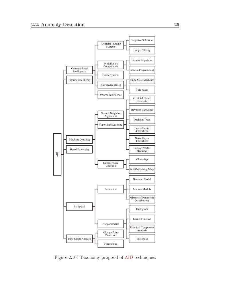
2.2. Anomaly Detection 25
����
#�&������������������ ��
������ ����&&��������&��
������������ �����
�������%�����
/����������#�&���������
,����� ��������&�
,����� �������&&����
*�$$�����&��
.�������!������
*�������������� ������
'��!"�����
����&��������� ��
�����&������%�����
�� ����� ��������
�������������"����������&��
����������� ��������
������ ������������������
�����������������
�� ������%�����
/���&"������#����������
�����������#����������
��������1� ������ ������
(������������ ��������
#���������
���!2�����$���������
��������� �������
�������� ��
����&���� �
,�������������
�������������
��0������������&���� �������"�������
�������&���� �
��������&�
.�����*�� �����
���� ����#�&��������������
%��������%�&����������������
#���������������� �����
*��� �������
Figure 2.10: Taxonomy proposal of AID techniques.

26 Chapter 2. State of the Art
extract meaningful statistics and other characteristics of the data. Although
it can be groped inside statistical, we have decided to locate it in a separate
branch because the viewpoint taken for AID may not be based on statistical
methods.
2.2.3 Anomaly Intrusion Detection Techniques
This section is devoted to provide a survey of the proposed techniques in AID.
Since the majority of the techniques rely on existing detecting paradigms as
presented in the taxonomy of Figure 2.10 and apply variations to them, we
will follow in this section the aforementioned classification and describe each
basic technique for each category, finally summarizing the different variations
proposed in the literature.
All these techniques are divided into two main steps. In the first step,
commonly denoted as the training phase, the AID technique builds a model
of the normal behavior based on training data. Then, in the second step,
anomalies are detected, and usually given an anomaly score, based on a
similarity measure of the test instances with the normal trained baseline.
This second step is denoted in the literature as testing phase.
Computational Intelligence
Computational intelligence (CI) is a fairly new research field of Nature-
inspired computational methodologies and approaches to address complex
problems of the real world applications. Although there is not yet full agree-
ment on what CI exactly is, there is a widely accepted view on which areas
belong to CI, which will be described next. The most accepted definition of
CI is given by Bezdek in [Bez92]:
A system is computational intelligent when it: deals with only
numerical (low-level) data, has pattern recognition components,
does not use knowledge in the artificial intelligence sense; and
additionally when it (begins to) exhibit (i) computational adap-
tivity, (ii) computational fault tolerance, (iii) speed approaching

2.2. Anomaly Detection 27
human-like turnaround, and (iv) error rates that approximate
human performance.
Artificial Immune Systems AISs try to mimic the Human Immune Sys-
tem (HIS), which is capable of protecting the body against damage from an
extremely large number of harmful pathogens without prior knowledge of the
structure of these pathogens [KBA+07].
Negative Selection: Negative Selection (NS) algorithms are based on
one specific aspect of the HIS: NS in the T-cell maturation process. NS elim-
inates inappropriate T-cells that bind to self antigens. This allows the HIS
to detect non-self antigens without mistakenly detecting self antigens. NS
algorithms consist of the following three steps: defining self, generating de-
tectors and monitoring the occurrence of anomalies. The self is defined as the
normal behavior of analyzed patterns in the monitored system. Secondly, the
algorithm generates a number of random patterns that are compared to the
self patterns. In the case of a pattern matching a self-pattern, such pattern
is not a useful detector and thus it is eliminated. Otherwise, it becomes a
detector. Finally, in the monitoring stage, when any of the detector patterns
match a monitored pattern, the monitored system is considered to be under
risk and an alert is placed [KBA+07].
NS-based methods entail a number of features that make them suitable
for AID. First, no prior knowledge of intrusions is required, which allows
to detect new kinds of anomalies. Second, the detection rate is tunable by
setting the number of generated detectors. Finally, detection is distributable,
which means that each detector can detect anomalies independently and
without communication with other detectors [DFH96].
Table 2.2 summarizes different approaches to AID based on NS algorithm.

28 Chapter 2. State of the Art
Table 2.2: Negative selection approaches to AID.
Technique Comments
Hofmeyr
and Forrest
[HF00]
They present LISYS, an architecture for detecting
anomalies using NS algorithm for binary detection gen-
eration.
Gonzalez et
al. [GDK02]
They present a technique to detect anomalies using
negative selection and classification.
Harmer et al.
[HWGL02]
NS applied to detect anomalies based on 28 TCP
packet header features and 16 features of UDP and In-
ternet Control Message Protocol (ICMP) packet head-
ers.
Dasgupta
and Gonzalez
[DG02]
They present two Artificial Immune System (AIS)-
based methods to detect anomalies: negative and pos-
itive characterization.
Gonzalez and
Dasgupta
[GD02b]
They propose a two-step approach for AID. First, a
NS algorithm is used to generate abnormal samples,
that are used jointly with normal ones in the training
of an artificial neural network. The proposed method
is compared with a self-organizing map.
Gonzalez and
Dasgupta
[GD03]
Network-based anomaly detection technique.
Gomez et al.
[GGD03]
They present a new technique for generating a set of
fuzzy rules that can characterize the non-self space (ab-
normal) using only self (normal) samples.
Esponda et al.
[EFH04]
They present a framework to evaluate positive and neg-
ative selection schemes.
Continued on next page

2.2. Anomaly Detection 29
Table 2.2 – continued from previous page
Technique Comments
Sarafijanovic
and Le
Boudec
[SLB05]
They investigate the use of an AIS to detect node mis-
behavior in a mobile ad hoc network using dynamic
source routing.
Powers and
He [PH08]
They propose a two-component hybrid model. The
first one uses an AIS to detect anomalies. The second
one uses self-organizing maps to classify the anomalies
detected by the AIS.
Greensmith et
al. [GFA08]
They present an AIS-based AID focused on the detec-
tion of port scanning using SYN packets.
Schmidt et al.
[SPL+09]
They present a framework to monitor smartphones and
remotely detect anomalies using self-organizing maps
and AIS techniques.
Danger Theory: In 1998, Burgess [Bur98] claimed that the self and
non-self distinction on which the NS algorithms are based was too simple
to model the whole HIS mechanism. Consequently, he proposed to use the
Danger theory [Mat94].
Danger theory argues that there must be discrimination beyond the self
and non-self distinction because the HIS only discriminates the self from
the non-self partially. As a consequence, Danger theory posits that it is
not the foreignness of the antigens what is important for immune detection,
but instead the relative danger of these antigens. In this way, the Danger
theory suggests that foreign invaders which are dangerous will induce the
generation of cellular molecules (danger signals) by initiating cellular stress
or cell death. Finally, this danger signal triggers the evaluation of potential

30 Chapter 2. State of the Art
antigens through negative selection. Aickelin et al. in [ABC+03] present the
first in-depth discussion on the application of Danger theory to ID.
Table 2.3 summarizes different approaches to AID based on Danger the-
ory.
Table 2.3: Danger theory approaches to AID.
Technique Comments
Burgess
[Bur00]
Cfengine: Open source configuration management
platform.
Begnum
and Burgess
[BB03]
Combine process homeostasis with Cfengine positive
and negative selection schemes.
Sarafijanovic
and Le
Boudec
[SLB04]
They present an AID system for wireless ad hoc net-
works that considers packet losses as a danger signal.
Greensmith et
al. [GAC05]
They employ DCs within AIS that coordinated T-cell
immune responses.
Kim et al.
[KWAM05]
They discuss T-cell immunity and tolerance for com-
puter worm detection.
Kim et al.
[KGTA05]
The artificial tissue, the Dendritic Cells (DC) algo-
rithm and T-cell algorithm were combined and pre-
sented as a different version of the danger theory in-
spired AISs.
Evolutionary Computation Evolutionary Computation (EC) is a sub-
field of CI that involves combinatorial optimization problems. EC uses iter-

2.2. Anomaly Detection 31
ative progress, such as growth or development in a population. This popu-
lation is then selected in a guided random search using parallel processing
to achieve the desired end. Such processes are often inspired by biological
mechanisms of evolution [WB10].
Genetic Algorithm: A Genetic Algorithm (GA) is a search heuristic
that mimics the process of natural evolution. This heuristic is routinely used
to generate useful solutions to search problems, such as finding anomalies
buried in the background traffic. GA is used in IDSs as optimization compo-
nents, for automatically modeling structure design or as classifiers [WB10].
In a GA, a population which encode candidate solutions to the target
problem evolves toward better solutions. The evolution usually starts from a
population of randomly generated individuals and happens in generations. In
each generation, the fitness of every individual in the population is evaluated,
multiple individuals are stochastically selected from the current population
based on their fitness, and modified (mutated) to form a new population.
The new population is then used in the next iteration of the algorithm.
Commonly, the algorithm terminates when either a maximum number of
generations has been produced, or a satisfactory fitness level has been reached
for the population. If the algorithm has terminated due to a maximum
number of generations, a satisfactory solution may or may not have been
reached. Consequently, a GA requires a genetic representation of the solution
and a fitness function to evaluate it.
Table 2.4 summarizes different approaches to AID based on GAs.
Table 2.4: Genetic algorithm approaches to AID.
Technique Comments
Mischiatti
and Neri
[MN00]
They learn network models using GAs, and compare
for discrepancies.
Continued on next page

32 Chapter 2. State of the Art
Table 2.4 – continued from previous page
Technique Comments
Balajinath
and Ragha-
van [BR01]
They use GAs to learn the individual user behavior and
detect anomalies by predicting current user behavior
based on past observations.
Gomez and
Dasgupta
[GD02a]
They present a methodology that allows the applica-
tion of fuzzy classifiers and genetic algorithms to AID.
Gomez et al.
[GDNG02]
The authors propose a new linear representation
scheme for evolving fuzzy rules using the concept of
complete binary tree structures and apply it to detect
network-based anomalies.
Hofmann et
al. [HSS03]
They use a GA to learn the structure of Radial Basis
Function (RBF) nets.
Pillai et al.
[PEV04]
They introduce the application of GAs, in order to im-
prove the effectiveness of IDSs.
Liu et al.
[LCLZ04]
They use genetic clustering to automatically establish
clusters and detect intruders by labeling normal and
abnormal groups.
Leon et al.
[LNG04]
They apply clustering to detect anomalies. The num-
ber of clusters is automatically determined by a GA.
Li [Li04] The author describes a technique of applying GAs to
network ID. The implementation considers both tem-
poral and spatial information of network connections.
Lu and Traore
[LT05]
They applied a GA to decide the number of clusters
based upon Gaussian mixture models.
Zhao et al.
[ZZL05]
They apply k-means to decide potential cluster centers
and a GA subsequently refined the centroids.
Continued on next page

2.2. Anomaly Detection 33
Table 2.4 – continued from previous page
Technique Comments
Gong et al.
[GZA05]
A GA is employed to derive a set of classification rules
from network audit data, and the support-confidence
framework is utilized as fitness function to judge the
quality of each rule.
Stein et al.
[SCWH05]
The authors propose an IDS that uses a GA to select
a subset of input features for decision tree classifiers,
thus improving the classification performance.
Abadeh et al.
[AHL07]
They propose an AID system based on fuzzy learning
using GAs.
Abadeh et al.
[SAHBS07]
They propose a method based on GAs to find fuzzy
rules.
Toosi and Ka-
hani [TK07]
They present a method to detect anomalies based on
three layers. One of them is based on GAs.
Ozyer et al.
[OAB07]
The authors propose an intelligent IDS that uses fuzzy
association rules mining to select classification rules
that are later used by a genetic fuzzy classifier.
Tsang et al.
[TKW07]
The authors present a novel ID approach that evolves
fuzzy-rules using GAs to detect network-based intru-
sions.
Genetic Programming: Genetic Programming (GP) is a specializa-
tion of GAs where each individual is a computer program. It is used to
optimize a population of computer programs according to a fitness land-
scape determined by a program’s ability to perform a given computational
task.

34 Chapter 2. State of the Art
GP evolves computer programs, traditionally represented in memory as
tree structures, which can be easily evaluated in a recursive manner. Every
tree node has an operator function and every terminal node has an operand,
making mathematical expressions easy to evolve and evaluate. Non-tree rep-
resentations have been suggested and successfully implemented, such as Lin-
ear Genetic Programming (LGP).
Table 2.5 summarizes different approaches to AID based on GP.
Table 2.5: Genetic programming approaches to AID.
Technique Comments
Song et al.
[SHZH03]
They propose page-based LGP with two-layer Sub-
set Selection to address a two-class intrusion detection
classification problem.
Lu and Traore
[LT04]
They present a rule evolution approach based on GP
for detecting novel attacks on networks.
Mukkamala et
al. [MSA04]
They present an AID approach based on LGP.
Song et al.
[SHZH05]
They present a methodology to filter features of a
dataset to its application to genetic programming.
Grosan et al.
[GAH05]
They present an AID system based on Multi-
Expression Programming.
Yin et al.
[YTHH05]
They present a GP-based rule learning approach for
detecting attacks on network.
Folino et al.
[FPS05]
They present an intrusion detection algorithm based
on GP ensembles.
Abraham
et al.
[AGMV07]
They present three variants of GP techniques to AID.
Continued on next page

2.2. Anomaly Detection 35
Table 2.5 – continued from previous page
Technique Comments
Chen et al.
[CAY07]
The authors present an IDS using a flexible multi-layer
Artificial Neural Network, which is evolved using the
probabilistic incremental program evolution algorithm
and whose features are selected using Particle Swarm
Optimization.
Fuzzy Systems FSs are based on fuzzy logic. Fuzzy logic, dealing with
the vague and imprecise, analyzes analog input values in terms of logical
variables that take on continuous values between 0 and 1, in contrast to
digital logic, which operates on discrete values of either 1 or 0 (true or false
respectively).
The input variables in a Fuzzy System (FS) are in general mapped into by
sets of membership functions, known as fuzzy sets. The process of converting
a crisp input value to a fuzzy value is called fuzzification. The microcontroller
makes decisions for what action to take based on a set of rules involving fuzzy
sets.
FSs consist of an input stage, a processing stage, and an output stage.
The input stage maps inputs to the appropriate membership functions and
truth values. The processing stage invokes each appropriate rule and gen-
erates a result for each, then combines the results of the rules. Finally, the
output stage converts the combined result back into a specific control output
value.
Table 2.6 summarizes different approaches to AID based on FSs.

36 Chapter 2. State of the Art
Table 2.6: Fuzzy system approaches to AID.
Technique Comments
Dickerson
and Dickerson
[DD00]
They present FIRE, an anomaly-based IDS that uses
fuzzy logic to assess whether malicious activity is tak-
ing place on a network.
Bridges and
Vaughn
[BV00]
They propose the use of fuzzy association rules and
fuzzy sequential rules to mine normal patterns from
audit data.
Luo and
Bridges
[LB00]
They build an AID system by comparing fuzzy rules
mined in the training phase with those mined from
new audit data.
Zhu et al.
[ZPZC01]
They present a comparison of three data mining tech-
niques for AID. They conclude that fuzzy sets provide
the best accuracy, followed by artificial neural networks
and rule-based techniques.
Florez et al.
[FBV02]
They propose a fuzzy rules comparison algorithm that
is amenable to on-line application.
Gomez et al.
[GDNG02]
The authors propose a new linear representation
scheme for evolving fuzzy rules using the concept of
complete binary tree structures and apply it to detect
network-based anomalies.
Gomez and
Dasgupta
[GD02a]
They present a methodology that allows the applica-
tion of fuzzy classifiers and genetic algorithms to AID.
Shah et al.
[SUJ03]
They present a fuzzy clustering (C-Mediods) approach
to AID.
Continued on next page

2.2. Anomaly Detection 37
Table 2.6 – continued from previous page
Technique Comments
Gomez et al.
[GGD03]
They present a new technique for generating a set of
fuzzy rules that can characterize the non-self space (ab-
normal) using only self (normal) samples.
Chavan et al.
[CSD+04]
The authors propose an IDS using artificial neural net-
works and fuzzy inference system.
El-Semary
et al.
[ESEGP05]
They propose an AID based on a fuzzy inference engine
to compare rules.
Chimphlee
et al.
[CANMS+06]
They present a fuzzy clustering (C-Means) approach
to AID.
Abadeh et al.
[AHL07]
They propose an AID system based on fuzzy learning
using genetic algorithm.
Abadeh et al.
[SAHBS07]
They propose a method based on GAs to find fuzzy
rules.
Toosi and Ka-
hani [TK07]
They present a method to detect anomalies based on
three layers. One of the is based on fuzzy logic.
Abraham et
al. [AJTH07]
They present a distributed AID system using fuzzy
classifiers.
Ozyer et al.
[OAB07]
The authors propose an intelligent IDS that uses fuzzy
association rules mining to select classification rules
that are later used by a genetic fuzzy classifier.
Tsang et al.
[TKW07]
The authors present a novel ID approach that evolves
fuzzy-rules using genetic algorithms to detect network-
based intrusions.

38 Chapter 2. State of the Art
Knowledge-Based A Knowledge-Based System (KBS) is a computer sys-
tem that emulates the decision-making ability of a human expert. KBSs are
designed to solve complex problems by reasoning about knowledge, like an
expert, and not by following the procedure of a developer as is the case in
conventional programming.
Finite State Machines: A Finite State Machine (FSM) is a mathe-
matical model used to design computer programs and digital logic circuits.
It is conceived as an abstract machine that can be in one of a finite number
of states. The machine is in only one state at a time (current state). It
can change from one state to another when initiated by a triggering event or
condition (transition). A particular FSM is defined by a list of the possible
transition states from each current state, and the triggering condition for
each transition.
Table 2.7 summarizes different approaches to AID based on FSMs.
Table 2.7: Finite state machines approaches to AID.
Technique Comments
Ghosh et al.
[GMS00]
They present two methods to detect anomalies. The
methods are based on artificial neural networks and
FSMs.
Sekar et al.
[SGF+02]
They present a method to detect anomalies based on
protocol modeling with FSMs.
Estevez-
Tapiador
et al.
[ETGTDV03]
They present a FSM model for TCP which is useful for
detecting anomalies through the use of Markov chains.
Treurniet
[Tre11]
The author presents a method to monitor Internet traf-
fic sessions using FSMs of the main protocols.

2.2. Anomaly Detection 39
Rule-Based: Rule-Based (RB) AID techniques learn rules that capture
the normal behavior of a system. A test instance that is not covered by any
such rule is considered as an anomaly. A basic RB technique consists of
two steps. The first step is to learn rules from the training data using a
rule learning algorithm. Each rule has an associated confidence value that
is proportional to the ratio of correctly classified training instances. The
second step is to find, for each test instance, the rule that best captures the
test instance. The inverse of the confidence associated with the best rule is
the anomaly score of the test instance.
Table 2.8 summarizes different approaches to AID based on RB.
Table 2.8: Rule-based approaches to AID.
Technique Comments
Lee et al.
[LSM00]
They propose to use the association rules and frequent
episodes computed from audit data to detect anoma-
lies.
Barbara et al.
[BCJW01]
They propose a system that implements several data
mining techniques to detect anomalies.
Zhu et al.
[ZPZC01]
They present a comparison of three data mining tech-
niques for AID. They conclude that fuzzy sets provide
the best accuracy, followed by artificial neural networks
and rule-based techniques.
Mahoney and
Chan [MC02]
They present a method that learn rules from attack-
free network traffic.
Mahoney and
Chan [MC03]
They present an algorithm (LERAD) that learns rules
for finding rare events in nominal time-series data with
long range dependencies.
Continued on next page

40 Chapter 2. State of the Art
Table 2.8 – continued from previous page
Technique Comments
Han and Cho
[HC03]
They present a rule-based model to integrate different
AID approaches.
Chan et al.
[CMA03]
They explore two methods for anomaly detection based
on past behavior. The first method is a rule learning
algorithm. The second method uses a clustering algo-
rithm to identify outliers.
Otey et al.
[OPG+03]
They present and evaluate a NIC-based network intru-
sion detection system. The AID system is rule-based.
Gomez et al.
[GGD03]
They present a new technique for generating a set of
fuzzy rules that can characterize the non-self space (ab-
normal) using only self (normal) samples.
Qin and
Hwang
[QH04]
They propose a new Internet trace technique for gen-
erating frequent episode rules to characterize Internet
traffic events.
Tandon and
Chan [TC07]
They propose the use of weights in the learned rules to
enhance LERAD.
Brauckhoff et
al. [BDWS09]
They propose the use of association rule mining to
find and summarize the flows related with the detected
anomalies.
Swarm Intelligence Swarm Intelligence (SI) is an CI technique involving
the study of collective behavior in decentralized systems. It computation-
ally emulates the emergent behavior of social insects or swarms in order to
simplify the design of distributed solutions to complex problems.
Generally speaking, SI models are population-based. Individuals in the
population are potential solutions. These individuals collaboratively search

2.2. Anomaly Detection 41
for the optimum through iterative steps. Individuals change their positions in
the search space, however, via direct or indirect communications, rather than
the crossover or mutation operators in evolutionary computation. Among the
SI methods, there are two that outstand: Ant Colony Optimization (ACO)
and Particle Swarm Optimization (PSO) [WB10].
Table 2.9 summarizes different approaches to AID based on SI.
Table 2.9: Swarm intelligence approaches to AID.
Technique Comments
Ramos and
Abraham
[RA05]
They present an ant-based clustering algorithm to de-
tect intrusion in a network infrastructure.
Tsang and
Kwong
[TK05]
They propose an improved version of the basic ant-
based clustering algorithm.
Abadeh et al.
[AHA06]
They embedded a standard PSO into their fuzzy ge-
netic algorithm.
Guolong et al.
[GQW07]
They propose the use of PSO to learn classification
rules.
He et al.
[HLC07]
They present an ant-classifier algorithm for discovering
classification rules.
Chen et al.
[CAY07]
The authors present an IDS using a flexible multi-layer
Artificial Neural Network, which is evolved using the
probabilistic incremental program evolution algorithm
and whose features are selected using PSO.

42 Chapter 2. State of the Art
Information Theory
Information theory is a branch of applied mathematics and electrical engi-
neering involving the quantification of information. A key measure of in-
formation, known as entropy, was proposed by Claude E. Shanon in 1948.
Entropy quantifies the uncertainty involved in predicting the value of a ran-
dom variable, and it has been applied to AID since, by hypothesis, anoma-
lies in data induce irregularities in the information content of the data set.
Consequently, measuring the information content in anomaly-free data and
comparing it to the entropy of test data is able to detect potential anomalies.
Table 2.10 summarizes different approaches to AID based on information
theory.
Table 2.10: Information theory approaches to AID.
Technique Comments
Lee and Xi-
ang [LX01]
They propose to use several information-theoretic mea-
sures, namely, entropy, conditional entropy, relative
conditional entropy, information gain, and information
cost for anomaly detection.
Gu et al.
[GMT05]
They introduce the detection of anomalies using the
maximum entropy which detect changes that point to
anomalies.
Lakhina et al.
[LCD05]
They present a method to detect anomalies in large
datasets through sample entropy.
Xu et al.
[XZB05]
They present a model to profile backbone traffic using
clustering and entropy.
Wagner and
Plattner
[WP05]
They present an application of entropy to detect worms
in the Internet.
Continued on next page

2.2. Anomaly Detection 43
Table 2.10 – continued from previous page
Technique Comments
Zuraniewski
and Rincon
[ZR06]
They propose two methods for detecting change points
in the network traffic fractality. The first one is based
on a cumulated sum (CUSUM) technique while the sec-
ond uses the Schwarz Information Criterion.
Nychis et al.
[NSA+08]
They evaluate entropy-based AID techniques. They
found that port and address distributions are highly
correlated.
Ashfaq et al.
[ARM+08]
They present a comparison of eight AID systems fo-
cused on detecting portscans. The best performance is
exhibited by entropy-based and threshold random walk
techniques.
Lee et al.
[LKK+08]
They propose a method for proactive detection of Dis-
tributed Denial of Service (DDoS) attacks using en-
tropy and clustering. The method is able to detect the
attacks in their initial stages.
Androulidakis
et al.
[ACP09]
They present a study of how to improve the sampling
process to reduce its impact on AID. They illustrate
their results with an entropy-based AID.
Burkhart et
al. [BSMD10]
They propose SEPIA, a library for multiparty compu-
tation that allows preserving privacy when aggregating
multi-domain network events and statistics. They illus-
trate the framework detecting anomalies using entropy
and thresholds.

44 Chapter 2. State of the Art
Machine Learning
Machine learning is a scientific discipline concerned with the design and de-
velopment of algorithms that allow computers to evolve behaviors based on
empirical data. A learner can take advantage of examples (data) to capture
characteristics of interest of their unknown underlying probability distribu-
tion. A major focus of machine learning research is to automatically learn
to recognize complex patterns and make intelligent decisions based on data.
Hence the learner must generalize (perform accurately on new, unseen ex-
amples after training on a finite data set) from the given examples, so as to
be able to produce a useful output in new cases. Quoting Tom M. Mitchell:
A computer program is said to learn from experience E with
respect to some class of tasks T and performance measure P, if
its performance at tasks in T, as measured by P, improves with
experience E [Mit97].
Nearest Neighbor Algorithms Nearest Neighbor (NN) algorithms are
based on the assumption that normal data instances are far from anomalous
data instances. Consequently, NN-based AID techniques require a distance
or similarity measure. For continuous attributes, Euclidean distance is a
popular choice.
The most popular algorithm uses the distance to the kth nearest neighbor
(k -NN). In this technique, an anomaly score proportionally inverse to the
distance to its kth nearest neighbor is assigned to new data instances. Finally,
a threshold, based either on the anomaly score or given by the mth largest
score, is used to determine which instances of the dataset are considered to
be anomalous.
Table 2.11 summarizes different approaches to AID based on nearest
neighbor algorithm.

2.2. Anomaly Detection 45
Table 2.11: Nearest neighbor algorithm approaches to
AID.
Technique Comments
Eskin et al.
[EAP+02]
They present three methods to detect anomalies, based
on nearest neighbors, clustering and support vector
machines, respectively.
Liao and Ve-
muri [LV02b]
They present a method to detect intrusions by moni-
toring executing programs. They use k -NN to detect
deviations of programs’ behavior.
Liao and Ve-
muri [LV02c]
They present a new approach, based on the k -NN clas-
sifier, to classify program behavior as normal or intru-
sive.
Dokas et al.
[DEK+02]
They present three methods to detect anomalies, based
on nearest neighbors, density based local outliers and
support vector machines, respectively.
Hu et al.
[HLV03]
They compare the performance of robust support vec-
tor machines with that of conventional support vector
machines and NN classifiers.
Lazarevic et
al. [LEK+03]
They compare different AID techniques, among which
they use k -NN.
Hautamaki et
al. [HKF04]
They present an outlier detection using indegree num-
ber algorithm that utilizes k -NN graph.
Patwari et al.
[PHIP05]
They use k -NN to reduce dimensionality of network
measurements to two dimensions thus providing a
mean for visualization of the relationships existing in
the data.
Continued on next page

46 Chapter 2. State of the Art
Table 2.11 – continued from previous page
Technique Comments
Ahmed et al.
[AOC07]
They investigate the use of the block-based One-Class
Neighbor Machine and the recursive Kernel-based On-
line Anomaly Detection algorithms for network ID.
Sharma et al.
[SPP07]
They present an IDS based on system call sequences
using text processing techniques. As similarity mea-
sure a kernel function is used, and k -NN classify the
processes as either normal or abnormal.
Li and Guo
[LG07]
The authors propose a novel supervised network ID
method based on transductive confidence machines for
k -NN.
Supervised Learning Supervised learning is the machine learning task
of inferring a function from supervised (labeled) training data. The training
data consist of a set of training examples and a desired output value. A
supervised learning algorithm analyzes the training data and produces an
inferred function. The inferred function should predict the correct output
value for any valid input object. Supervised learning techniques have been
numerously applied to AID, although it is hard to properly label training
data. Typically, attack-free data are used for the training phase, and the
paradigms flag unseen patterns as anomalous.
Artificial Neural Networks: An Artificial Neural Network (ANN) is
a mathematical model that is inspired by the structure and functional aspects
of biological neural networks. An ANN consists of an interconnected group
of artificial neurons, which changes its structure based on information that
flows through the network during the learning phase. They are typically

2.2. Anomaly Detection 47
used to model complex relationships between inputs and outputs or to find
patterns in data.
A basic ANN operates in two steps. First, an ANN is trained on the
normal training data to learn the normal classes. Second, each test instance
is provided as an input to the ANN. If the ANN accepts the test input, it is
normal and it is an anomaly on the contrary.
Table 2.12 summarizes different approaches to AID based on artificial
neural network.
Table 2.12: Artificial neural network approaches to AID.
Technique Comments
Ghosh et al.
[GMS00]
They present two methods to detect anomalies. The
methods are based on ANNs and finite state machines.
Lee and Hein-
buch [LH01]
They present a method to detect protocol misuse using
hierarchical neural networks.
Zhu et al.
[ZPZC01]
They present a comparison of three data mining tech-
niques for AID. They conclude that fuzzy sets provide
the best accuracy, followed by ANNs and rule-based
techniques.
Manikopoulos
and Papavas-
siliou [MP02]
They present a method to detect anomalies using a
distribution comparator. The comparisons are joined
with a neural network.
Gonzalez and
Dasgupta
[GD02b]
They propose a two-step approach for AID. First, a
negative selection algorithm is used to generate abnor-
mal samples, that are used jointly with normal ones
in the training of an ANN. The proposed method is
compared with a self-organizing map.
Continued on next page

48 Chapter 2. State of the Art
Table 2.12 – continued from previous page
Technique Comments
Mukkamala et
al. [MJS02]
They describe two approaches to AID, one using sup-
port vector machines and other using ANNs. In ad-
dition, they show an approach for data reduction, ex-
hibiting its performance with the proposed models.
Sung and
Mukkamala
[SM03]
They perform experiments to identify which are the
most interesting features of DARPA datasets (§2.2.4)for the identification of the different traffic kinds.
Joo et al.
[JHH03]
They propose a method that uses the neural network
model for AID but consider the cost ratio of false neg-
ative errors to false positive errors to enhance the ef-
fectiveness of the intrusion detection.
Li and
Manikopoulos
[LM03]
The authors present MAID, a histogram-based AIDSs
that uses ANN classifiers to detect Denial of Service
(DoS) attacks using MIB traffic parameters.
Moradi and
Zulkernine
[MZ04]
They present a a model to classify anomalies in three
classes (one of them is normal traffic) using a multilayer
neural network.
Chavan et al.
[CSD+04]
The authors propose an IDS using ANN and fuzzy in-
ference system.
Corchado et
al. [CHS05b]
They present a method to detect anomalies by project-
ing features using neural networks.
Chen et al.
[CHS05a]
They compare ANNs and support vector machines to
detect anomalies on business service management au-
dit data. They conclude that support vector machines
outperform ANNs.
Continued on next page

2.2. Anomaly Detection 49
Table 2.12 – continued from previous page
Technique Comments
Zhang et al.
[ZJK05]
They present two hierarchical frameworks to detect
intrusions based on modular neural networks trained
with RBFs.
Mukkamala et
al. [MSA05]
They present three methods to detect anomalies based
on artificial neural networks, support vector machines
and multivariate adaptive regression splines. Then
they build a new detector joining the previous ones,
which outperforms them.
Gavrilis and
Dermatas
[GD05]
They present and evaluate a RBF neural network de-
tector for DDoS attacks in public networks based on
statistical features estimated in short-time windows of
the incoming data packets.
Han and Cho
[HC06]
They use evolutionary neural networks to detect
anomalies.
Amini et al.
[AJS06]
They present a framework to detect intrusions using
different kinds of neural networks.
Florez-
Larrahondo
et al.
[FLLD+06]
They propose the integration of intelligent anomaly de-
tection agents for distributed monitoring. They moni-
tor operating system calls with neural network models
and function calls with hidden Markov models.
Faraoun
and Boukelif
[FB07]
They present a method to detect anomalies using neu-
ral networks that uses k -means clustering to improve
the training phase.
Chen et al.
[CAY07]
The authors present an IDS using a flexible multi-layer
ANN, which is evolved using the probabilistic incre-
mental program evolution algorithm and whose fea-
tures are selected using Particle Swarm Optimization.
Continued on next page

50 Chapter 2. State of the Art
Table 2.12 – continued from previous page
Technique Comments
Liu et al.
[LYY07]
The authors propose a hybrid IDS using principal com-
ponent analysis neural networks.
Corchado
and Herrero
[CH11]
They present a methodology to visualize network traffic
that is able to expose the anomalies present in such
traffic.
Bayesian Networks: A Bayesian Network (BN) is a probabilistic graph-
ical model that represents a set of random variables and their conditional de-
pendencies via a Directed Acyclic Graph (DAG). The nodes of such DAG rep-
resent random variables in the Bayesian sense. Edges represent conditional
dependencies—nodes which are not connected represent variables which are
conditionally independent of each other. Each node is associated with a prob-
ability function that takes as input a particular set of values for the node’s
parent variables and gives the probability of the variable represented by the
node.
Given a test data instance, the model estimates the posterior probability
of the test instance belonging to the normal and anomaly classes, based on
the training data. The class with the largest posterior probability is chosen
as the predicted class for the given test instance.
Table 2.13 summarizes different approaches to AID based on Bayesian
networks.

2.2. Anomaly Detection 51
Table 2.13: Bayesian networks approaches to AID.
Technique Comments
Valdes and
Skinner
[VS00]
They present an adaptive, model-based technique for
attack detection, using Bayes networks technology to
analyze bursts of traffic.
Ye et al.
[YXE00]
They present a method based on Bayesian probabilistic
network to detect network anomalies.
Barbara et al.
[BWJ01]
They propose a method based on a technique called
pseudo-Bayes estimators to enhance an anomaly de-
tection systems ability to detect new attacks while re-
ducing the false alarm rate as much as possible.
Bronstein et
al. [BDD+01]
They propose a general architecture and implementa-
tion for the autonomous assessment of health of arbi-
trary service elements using Bayesian networks.
Sebyala et al.
[SOS02]
They present the application of Bayesian technology
in the development of an anomaly detection system for
proxylets.
Kruegel et al.
[KMRV03]
They present a method to detect anomalies based
Bayesian classifiers aggregated in a Bayesian network.
Mutz et al.
[MVVK06]
They present a host-based AID system based on several
models of system call arguments. The different models
are joined using a Bayesian network.
Decision Trees: A Decision tree is a decision support tool that uses
a tree-like graph of decisions and their possible consequences. Decision tree
learning uses a decision tree as a predictive model which maps observations
about an instance to conclusions about the instance’s target value. In these

52 Chapter 2. State of the Art
tree structures, leaves represent class labels and branches represent conjunc-
tions of features that lead to those class labels.
Table 2.14 summarizes different approaches to AID based on decision
trees.
Table 2.14: Decision trees approaches to AID.
Technique Comments
Li and Ye
[LY01]
They present a model to detect anomalies based on
decision trees. The trees are trained using past data
with anomalies.
Amor et al.
[ABE04]
They present two models and compare their perfor-
mance using DARPA datasets(§2.2.4). The methods
are naive Bayes classifier and decision trees.
Peddabachigari
et al. [PAT04]
The authors compare IDSs based on decision trees and
support vector machines. They show that decision
trees give better overall performance than support vec-
tor machines.
Kang et al.
[KFH05]
They present a new model for representing system calls
and test its efficiency when applied to AID.
Depren et al.
[DTAC05]
They present a hybrid model for intrusion detection. A
self-organizing map and a decision tree are joined with
a rule-based decision support system.
Stein et al.
[SCWH05]
The authors propose an IDS that uses a genetic algo-
rithm to select a subset of input features for decision
tree classifiers, thus improving the classification perfor-
mance.
Continued on next page

2.2. Anomaly Detection 53
Table 2.14 – continued from previous page
Technique Comments
Gaddam et al.
[GPB07]
They present a two-step method to detect anomalies.
First they apply k -means clustering to cluster the data,
and then they apply ID3 decision to detect subgroups
within each cluster.
Peddabachigari
et al.
[PAGT07]
They present four different methods based on different
intelligent system approaches to detect anomalies.
Xiang et al.
[XYM08]
They propose a multiple-level hybrid classifier for ID
that combines tress classifiers and Bayesian clustering.
Ensemble of Classifiers: Ensemble of Classifiers (EoC) methods use
multiple models to obtain better predictive performance than could be ob-
tained from any of the constituent models. The objective is to combine the
different models in order to enhance their benefits while diminishing their
drawbacks. In addition, different models can provide complementary infor-
mation about the patterns to be classified.
Table 2.15 summarizes different approaches to AID based on ensembles
of classifiers.
Table 2.15: Ensembles of classifiers approaches to AID.
Technique Comments
Bass [Bas00] The author surveys IDSs requirements. He points that
future IDSs would base their decisions on data fusion.
Continued on next page

54 Chapter 2. State of the Art
Table 2.15 – continued from previous page
Technique Comments
Manikopoulos
and Papavas-
siliou [MP02]
They present a method to detect anomalies using a
distribution comparator. The comparisons are joined
with a neural network.
Han and Cho
[HC03]
They present a rule-based method to integrate different
anomaly detection models. The final system is more
robust to false positives.
Siaterlis and
Maglaris
[SM04]
They present a method to integrate different denial of
service attack detection mechanisms.
Mukkamala et
al. [MSA05]
They present three methods to detect anomalies based
on artificial neural networks, support vector machines
and multivariate adaptive regression splines. Then
they build a new detector joining the previous ones,
which outperforms them.
Shifflet
[Shi05]
The author presents a model, independent of the AID
techniques, to fusion alerts and information.
Mutz et al.
[MVVK06]
They present a host-based AID system based on several
models of system call arguments. The different models
are joined using a Bayesian network.
Peddabachigari
et al.
[PAGT07]
They present four different methods based on different
intelligent system approaches to detect anomalies. The
ensemble of all the methods has the best performance.
Zhou et al.
[ZHR+07]
They propose a method to fusion alerts from different
intrusion detection systems.
Continued on next page

2.2. Anomaly Detection 55
Table 2.15 – continued from previous page
Technique Comments
Giacinto et al.
[GPDRR08]
They present a method to detect anomalies by creating
a classifier for each traffic kind and fusing the informa-
tion of such classifiers.
Naive Bayes Classifiers: A Naive Bayes Classifier (NBC) is a sim-
ple probabilistic classifier based on applying Bayes’ theorem with strong
(naive) independence assumptions. This means that a NBC assumes that
the presence/absence of a particular feature of a class is unrelated to the
presence/absence of any other feature, given the class variable.
An advantage of the NBCs is that it only requires a small amount of
training data to estimate the parameters necessary for classification. Be-
cause independent variables are assumed, only the variances of the variables
for each class need to be determined and not the entire covariance matrix.
Despite of its simplicity, NBCs have shown remarkable performance in com-
plex problems.
Table 2.16 summarizes different approaches to AID based on naive Bayes
classifier.
Table 2.16: Naive Bayes classifier approaches to AID.
Technique Comments
Schultz et al.
[SEZS01]
The authors propose a method for detecting new ma-
licious executables using different classifiers. The best
performance is obtained through NBCs.
Kruegel et al.
[KMRV03]
They present a method to detect anomalies based
Bayesian classifiers aggregated in a Bayesian network.
Continued on next page

56 Chapter 2. State of the Art
Table 2.16 – continued from previous page
Technique Comments
Axelsson
[Axe04]
The author presents a method to detect anomalies us-
ing a Bayesian classifier with interactive training for
reducing the false positive rate.
Amor et al.
[ABE04]
They present two models and compare their perfor-
mance using DARPA datasets(§2.2.4). The methods
are naive Bayes classifier and decision trees.
Kang et al.
[KFH05]
They present a new model for representing system calls
and test its efficiency when applied to AID.
Support Vector Machines: A Support Vector Machine (SVM) is a
concept in statistics and computer science for a set of related supervised
learning methods that analyze data and recognize patterns, used for classi-
fication and regression analysis. The basic SVM takes a set of input data
and predicts, for each given input, which of two possible classes forms the
input, making SVMs a non-probabilistic binary linear classifier. Given a
set of attack-free training examples, an SVM training algorithm builds a
model that determines whether new examples lie within the learned region
or outside its boundaries. Kernels, such as RBF kernel, can be used to learn
complex regions.
Table 2.17 summarizes different approaches to AID based on support
vector machines.

2.2. Anomaly Detection 57
Table 2.17: Support vector machines approaches to AID.
Technique Comments
Dokas et al.
[DEK+02]
They present three methods to detect anomalies, based
on nearest neighbors, density based local outliers and
SVMs, respectively.
Eskin et al.
[EAP+02]
They present three methods to detect anomalies, based
on nearest neighbors, clustering and SVMs, respec-
tively.
Mukkamala et
al. [MJS02]
They describe two approaches to AID, one using SVMs
and other using artificial neural networks. In addition,
they show an approach for data reduction, exhibiting
its performance with the proposed models.
Hu et al.
[HLV03]
They compare the performance of Robust SVMs with
that of conventional SVM and nearest neighbors clas-
sifiers.
Lazarevic et
al. [LEK+03]
They compare different AID techniques, among which
they use SVMs.
Heller et al.
[HSKS03]
They present a host-based IDS that monitors accesses
to the Microsoft Windows Registry using SVMs.
Sung and
Mukkamala
[SM03]
They perform experiments to identify which are the
most interesting features of DARPA datasets (§2.2.4)for the identification of the different traffic kinds.
Kim and Park
[KP03]
They propose and evaluate a network-based IDS using
SVMs.
Laskov et al.
[LSK04]
They propose a novel formulation of a one-class SVM
specially designed for typical IDSs data features.
Continued on next page
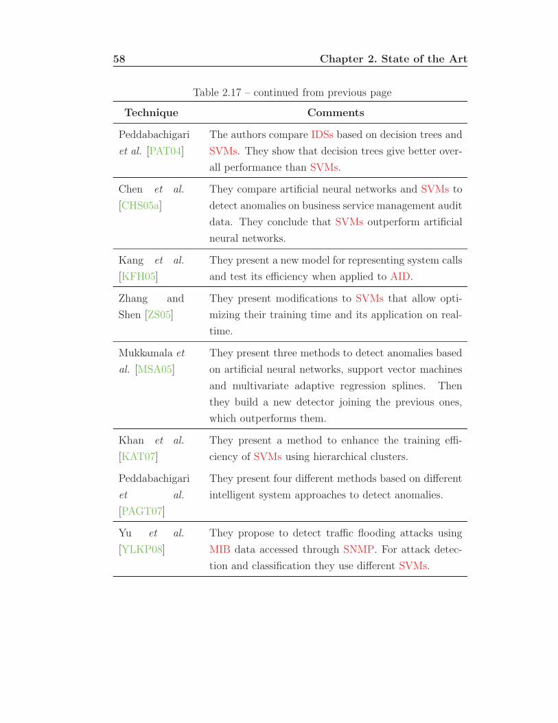
58 Chapter 2. State of the Art
Table 2.17 – continued from previous page
Technique Comments
Peddabachigari
et al. [PAT04]
The authors compare IDSs based on decision trees and
SVMs. They show that decision trees give better over-
all performance than SVMs.
Chen et al.
[CHS05a]
They compare artificial neural networks and SVMs to
detect anomalies on business service management audit
data. They conclude that SVMs outperform artificial
neural networks.
Kang et al.
[KFH05]
They present a new model for representing system calls
and test its efficiency when applied to AID.
Zhang and
Shen [ZS05]
They present modifications to SVMs that allow opti-
mizing their training time and its application on real-
time.
Mukkamala et
al. [MSA05]
They present three methods to detect anomalies based
on artificial neural networks, support vector machines
and multivariate adaptive regression splines. Then
they build a new detector joining the previous ones,
which outperforms them.
Khan et al.
[KAT07]
They present a method to enhance the training effi-
ciency of SVMs using hierarchical clusters.
Peddabachigari
et al.
[PAGT07]
They present four different methods based on different
intelligent system approaches to detect anomalies.
Yu et al.
[YLKP08]
They propose to detect traffic flooding attacks using
MIB data accessed through SNMP. For attack detec-
tion and classification they use different SVMs.

2.2. Anomaly Detection 59
Unsupervised Learning Unsupervised learning refers to the problem of
trying to find hidden structure in unlabeled data. Since the examples given
to the learner are unlabeled, there is no ground-truth to evaluate a potential
solution. This distinguishes unsupervised learning from supervised learning
and reinforcement learning.
Clustering: Clustering is the task of assigning a set of objects into
groups so that the objects in the same cluster are more similar to each other
than to those in other clusters.
Clustering can be achieved by various algorithms that differ significantly
in their notion of what constitutes a cluster and how to efficiently find them.
Popular notions of clusters include groups with low distances among the clus-
ter members, dense areas of the data space, intervals or particular statistical
distributions.
To detect anomalies using clustering, a clustering algorithm and a simi-
larity measure must be chosen. The most popular similarity measure is the
Euclidean distance. The clustering algorithm builds the clusters based on
the similarity distance. The anomalies are determined by the instances that
do not belong to any cluster, the instances that are far from their cluster
centroids, or data instances that belong to small or sparse clusters. The
interested reader is deferred to [CBK09, Section 6.1] for a discussion of the
differences between nearest neighbor and clustering paradigms.
Table 2.18 summarizes different approaches to AID based on clustering.
Table 2.18: Clustering approaches to AID.
Technique Comments
Portnoy et al.
[PES01]
They present a method to detect anomalies based on
clustering.
Ye and Li
[YL01]
They present a method based on clustering and classi-
fication to recognize intrusion signatures.
Continued on next page

60 Chapter 2. State of the Art
Table 2.18 – continued from previous page
Technique Comments
Taylor and
Alves-Foss
[TAF02]
They evaluate with real data an network-based AID
system based on clustering.
Eskin et al.
[EAP+02]
They present three methods to detect anomalies, based
on nearest neighbors, clustering and support vector
machines, respectively.
Sequeira and
Zaki [SZ02]
They present a host-based anomaly detection model
which uses clustering to detect anomalous events.
Gomez et al.
[GDN03]
The authors present a novel unsupervised robust clus-
tering technique based on the Gravitational Law and
the second Newton’s motion Law and apply it to
network-based AID.
Zanero and
Savaresi
[ZS04]
They present a two-tier architecture to detect anoma-
lies. The first layer summarizes the packet payload in-
formation, whereas the second layer detects and signals
anomalies.
Liu et al.
[LCLZ04]
They use genetic clustering to automatically establish
clusters and detect intruders by labeling normal and
abnormal groups.
Lakhina et al.
[LCD05]
They present a method to detect anomalies in large
datasets through sample entropy. The detected anoma-
lies are classified using clustering.
Xu et al.
[XZB05]
They present a model to profile backbone traffic using
clustering and entropy.
Kang et al.
[KFH05]
They present a new model for representing system calls
and test its efficiency when applied to AID.
Continued on next page

2.2. Anomaly Detection 61
Table 2.18 – continued from previous page
Technique Comments
Leung and
Leckie [LL05]
They present a method to detect anomalies using den-
sity and grid-based clustering.
Jiang et al.
[JSW+06]
They present CBUID, a clustering-based method for
the unsupervised intrusion detection.
Khan et al.
[KAT07]
They present a method to enhance the training effi-
ciency of SVMs using hierarchical clusters.
Faraoun
and Boukelif
[FB07]
They present a method to detect anomalies using neu-
ral networks that uses k -means clustering to improve
the training phase.
Gaddam et al.
[GPB07]
They present a two-step method to detect anomalies.
First they apply k -means clustering to cluster the data,
and then they apply ID3 decision to detect subgroups
within each cluster.
Zhong et al.
[ZKS07]
They investigate multiple unsupervised clustering al-
gorithms for AID: k -means, mixture of spherical Gaus-
sians and self-organizing map among others.
Lee et al.
[LKK+08]
They propose a method for proactive detection of
DDoS attacks using entropy and clustering. The
method is able to detect the attacks in their initial
stages.
Xiang et al.
[XYM08]
They propose a multiple-level hybrid classifier for ID
that combines tress classifiers and Bayesian clustering.
Self-Organizing Maps: A Self-Organizing Map (SOM) is a type of
artificial neural network that is trained using unsupervised learning to pro-
duce a low-dimensional, discretized representation of the input space of the

62 Chapter 2. State of the Art
training samples, called a map. This makes SOMs useful for visualizing
low-dimensional views of high-dimensional data, akin to multidimensional
scaling. The model was first described as an artificial neural network by
the Finnish professor Teuvo Kohonen, and therefore it is sometimes called a
Kohonen map [Koh82].
Like most artificial neural networks, SOMs operate in two modes: train-
ing and mapping. Training builds the map using input examples. It is a
competitive process, also called vector quantization. Mapping automatically
classifies a new input vector.
Table 2.19 summarizes different approaches to AID based on self-organizing
maps.
Table 2.19: Self-organizing maps approaches to AID.
Technique Comments
Rhodes et al.
[RMC00]
They use SOMs to recognize anomalies in computer
network data stream.
Lichodzijewski
et al.
[LZHH02a]
They present an AID system based on a SOM.
Lichodzijewski
et al.
[LZHH02b]
They present a host-based unsupervised AID method
using a SOM on user session’s information.
Labib and Ve-
muri [LV02a]
They present a method to detect anomalies based on
a SOM that allows results visualization.
Gonzalez and
Dasgupta
[GD02b]
They propose a two-step approach for AID. First, a
negative selection algorithm is used to generate abnor-
mal samples, that are used jointly with normal ones in
the training of an artificial neural network. The pro-
posed method is compared with a SOM.
Continued on next page

2.2. Anomaly Detection 63
Table 2.19 – continued from previous page
Technique Comments
Kayacik et al.
[KZHH03]
They present a method based on 6 SOMs, one for each
analyzed feature, to detect anomalies.
Ramadas et
al. [ROT03]
They present an AID model based on a SOM and apply
it to a six-tuple of network features.
Zanero and
Savaresi
[ZS04]
They present a two-tier architecture to detect anoma-
lies. The first layer summarizes the packet payload in-
formation, whereas the second layer detects and signals
anomalies.
Zanero
[Zan05]
They present a method to detect anomalies by moni-
toring TCP traffic patterns using a SOM.
Sarasamma et
al. [SZH05]
They present an AID system using a hierarchical SOM.
Depren et al.
[DTAC05]
They present a hybrid model for intrusion detection. A
SOM and a decision tree are joined with a rule-based
decision support system.
Vokorokos et
al. [VBC06]
They present an AID system using a SOM.
Bolzoni et al.
[BEH06]
They present a two-tier AID system. The first layer
uses a SOM to classify network traffic while the second
uses PAYL [WS04] to detect the anomalies.
Amini et al.
[AJS06]
They present a framework to detect intrusions using
different kinds of neural networks.
Wang et al.
[WGZY06]
They present two methods for host-based anomaly
detection by creating application profiles. The first
method is based on hidden Markov models while the
second is based on a SOM.
Continued on next page

64 Chapter 2. State of the Art
Table 2.19 – continued from previous page
Technique Comments
Kayacik et al.
[KZHH07]
They present an AID system using a hierarchical SOM.
Zhong et al.
[ZKS07]
They investigate multiple unsupervised clustering al-
gorithms for AID: k -means, mixture of spherical Gaus-
sians and SOMs among others.
Greensmith et
al. [GFA08]
They present an AIS-based AID focused on the detec-
tion of port scanning using SYN packets, and compare
it with a solution based on a SOM.
Powers and
He [PH08]
They propose a two-component hybrid model. The
first one uses an artificial immune system to detect
anomalies. The second one uses SOMs to classify the
anomalies detected by the artificial immune system.
Zanero and
Serazzi [ZS08]
They present a two-tier AID system. The first layer
uses a SOM to classify network traffic while the second
uses outlier detection to detect the anomalies.
Schmidt et al.
[SPL+09]
They present a framework to monitor smartphones and
remotely detect anomalies using a SOM and artificial
immune system techniques.
Signal Processing
Signal processing deals with operations on or analysis of signals, in either
discrete or continuous time. Signals of interest can include sound, images,
time-varying measurement values and sensor data. Signals are analog or
digital electrical representations of time-varying or spatial-varying physical
quantities.

2.2. Anomaly Detection 65
The most applied signal processing technique to detect anomalies is based
on the wavelet transform. The wavelet transform is a representation of a
signal by a combination of square-integrable functions, which is very useful
for detecting abrupt changes in the analyzed signals.
Table 2.20 summarizes different approaches to AID based on signal pro-
cessing.
Table 2.20: Signal processing approaches to AID.
Technique Comments
Barford
and Plonka
[BP01]
They present their intention to build a framework to
obtain and analyze anomalies based on flow-level net-
work traces, and present their main characteristics.
Thottan and
Ji [TJ03]
They present a method to detect anomalies based on
statistical signal processing technique based on abrupt
change detection.
Zhang et al.
[ZGGR05]
They introduce the term anomography, which is the
union of anomaly detection using tomographic data.
They present and compare different techniques.
Dainotti et al.
[DPV06b]
They propose a two-tier architecture to detect anoma-
lies. In the first layer two conservative are used to point
to possible anomalies. In the detectors second layer, a
continuous wavelet transform is used to determine the
time instant of the anomaly and its duration.
Zheng and Hu
[ZH06]
They present a method based on vector quantization,
a technique used in image compression.
Kyriakopoulos
and Parish
[KP07]
They use the wavelet transform to detect anomalies at
different timescales. Anomalies are detected as abrupt
signal changes.
Continued on next page

66 Chapter 2. State of the Art
Table 2.20 – continued from previous page
Technique Comments
Lu and Ghor-
bani [LG09]
They propose an AID system using wavelets and Gaus-
sian mixture models. They define 15 network features
that are able to model the normal network situation.
Then, using wavelets and an autoregressive model they
fit the time series of the characteristics. The residuals
of the regression are used to detect the anomalies.
Silveira et al.
[SDTG10]
They propose ASTUTE, a threshold-based AID tech-
nique focused on detecting correlated flows. They
compare the performance of ASTUTE with two alter-
nate anomaly detectors based on Kalman filters and
wavelets.
Statistical
Statistical AID methods rely on statistics to detect anomalous events. Statis-
tics is the study of the collection, organization, analysis, and interpretation of
data. The underlying principle of any statistical anomaly detection technique
is, quoting Anscombe and Guttman [AG60]:
An anomaly is an observation which is suspected of being
partially or wholly irrelevant because it is not generated by the
stochastic model assumed.
Statistical techniques fit a statistical model (usually for normal behavior)
to the given data and then apply a statistical inference test to determine if
an unseen instance belongs to this model or not.

2.2. Anomaly Detection 67
Parametric Parametric statistics is a branch of statistics that assumes
that the data have come from a type of probability distribution and makes
inferences about the parameters of the distribution. Parametric methods
establish more assumptions than non-parametric methods. If those extra
assumptions are correct, parametric methods can produce more accurate and
precise estimates. However, if those assumptions are incorrect, parametric
methods can be very misleading.
Gaussian Model: The Gaussian distribution is a two-parameter con-
tinuous probability distribution that has a bell-shaped probability density
function. The Gaussian distribution is considered the most prominent prob-
ability distribution in statistics: it is very tractable analytically, arises as the
outcome of the central limit theorem and the bell shape of the normal distri-
bution makes it a convenient choice for modeling a large variety of random
variables encountered in practice.
Gaussian model-based techniques fit a Gaussian distribution to anomaly-
free data. The parameters are commonly estimated using maximum likeli-
hood estimation [Ald97]. The anomaly score for a data instance is the inverse
of the probability of that instance being generated by the fitted model, and
a threshold is set to determine the anomalies.
Table 2.21 summarizes different approaches to AID based on Gaussian
models.
Table 2.21: Gaussian model approaches to AID.
Technique Comments
Yamanishi
and Takeuchi
[YT01]
They propose an AID method that uses a Gaussian
mixture model as a statistical representation of normal
behaviors.
Ye et al.
[YECV02]
They present an AID system based on a multivariate
Gaussian model. They use the Hotelling’s T2 test to
detect mean-shift anomalies.
Continued on next page

68 Chapter 2. State of the Art
Table 2.21 – continued from previous page
Technique Comments
Mutz et al.
[MVVK06]
They present a host-based AID system based on several
models of system call arguments. The different models
are joined using a Bayesian network.
Robertson et
al. [RVK+06]
They use different AID models to develop an AID sys-
tem. One of the methods uses a Gaussian distribution
to model attribute length. The system is applied to
detect web-based attacks.
Zhong et al.
[ZKS07]
They investigate multiple unsupervised clustering al-
gorithms for AID: k-means, mixture of spherical Gaus-
sians and self-organizing map among others.
Chhabra et al.
[CSKC08]
They present a method to detect network-wide anoma-
lies with sparse communication between monitors. The
method is based on the quantiles of traffic distributions
after Gaussian modeling.
Lu and Ghor-
bani [LG09]
They propose an AID system using wavelets and Gaus-
sian mixture models. They define 15 network features
that are able to model the normal network situation.
The, using wavelets and an autoregressive model they
fit the time series of the characteristics. The residuals
of the regression are used to detect the anomalies.
Markov Models: A Markov model is a stochastic model that assumes
the Markov property. A stochastic process has the Markov property, also
known as memoryless property, if the conditional probability distribution of
future states of the process (conditional on both past and present values)
depends only upon the present state; that is, given the present, the future
does not depend on the past.

2.2. Anomaly Detection 69
The most popular Markov models are Markov chains and HMMs. A
Markov chain is a mathematical system that undergoes transitions from one
state to another, between a finite or countable number of possible states.
It is a random process characterized by the Markov property. A Hidden
Markov Model (HMM) is a statistical Markov model in which the system
being modeled is assumed to be a Markov process with unobserved (hidden)
states. In a regular Markov model, the state is directly visible to the observer,
and therefore the state transition probabilities are the only parameters. In a
HMM, the state is not directly visible, but output, dependent on the state,
is visible. Each state has a probability distribution over the possible output
tokens. Therefore the sequence of tokens generated by a HMM gives some
information about the sequence of states.
Table 2.22 summarizes different approaches to AID based on Markov
models.
Table 2.22: Markov model approaches to AID.
Technique Comments
Lane and
Brodley
[LB03]
They introduce two approaches to AID: one employing
instance-based learning and the other using HMMs.
Estevez-
Tapiador
et al.
[ETGTDV03]
They present a finite state machine model for TCP
which is useful for detecting anomalies through the use
of Markov chains.
Yeung and
Ding [YD03]
They present two methods to detect host-based anoma-
lies. System calls are modeled using a HMM or fre-
quency distributions (histograms).
Wang et al.
[WGZ04b]
They present a model for detecting anomalies by ana-
lyzing system call logs using HMMs.
Continued on next page

70 Chapter 2. State of the Art
Table 2.22 – continued from previous page
Technique Comments
Ye et al.
[YZB04]
They present the application of Markov chains to
anomalies by building a model for system activity tran-
sitions.
Estevez-
Tapiador
et al.
[ETGTDV05]
They present a method based on the monitoring of in-
coming HTTP request to detect attacks against web
servers. The detection is accomplished through a
Markovian model.
Khanna and
Liu [KL06]
They present a method to detect anomalies on mobile
ad-hoc networks using a HMM.
Wang et al.
[WGZY06]
They present two methods for host-based anomaly
detection by creating application profiles. The first
method is based on HMMs while the second is based
on a self-organizing map.
Mutz et al.
[MVVK06]
They present a host-based AID system based on several
models of system call arguments. The different models
are joined using a Bayesian network.
Florez-
Larrahondo
et al.
[FLLD+06]
They propose the integration of intelligent anomaly de-
tection agents for distributed monitoring. They moni-
tor operating system calls with neural network models
and function calls with HMMs.
Paschalidis
and Smarag-
dakis [PS09]
They propose two methods to on-line spatial AID.
One is model-based using a Markov modulated process
whereas the other is model-free.
Mixture of Parametric Distributions: A mixture model is a prob-
abilistic model for representing the presence of subpopulations within an

2.2. Anomaly Detection 71
overall population, without requiring that an observed dataset should iden-
tify the subpopulation to which an individual observation belongs. Generally,
mixture models are used to make statistical inferences about the properties of
the subpopulations given only observations on the pooled population, with-
out subpopulation-identity information.
There are two possible approaches using mixture models. The first one
use a set of distributions to model the normal behavior, while using a differ-
ent set of distributions to model the anomalous behavior. Then, new data
instances are assigned to any of the distributions based on their likelihood,
and in the case such distribution is used to model the anomalous behavior,
data instances are flagged as anomalous. The second approach only models
the normal instances as a mixture of parametric distributions, and the data
instances that have low likelihood of belonging to the any of the distributions
are reported as anomalous.
Table 2.23 summarizes different approaches to AID based on mixtures of
parametric distributions.
Table 2.23: Mixture of parametric distributions ap-
proaches to AID.
Technique Comments
Eskin [Esk00] They present a method to detect anomalies using a
mixture model for explaining the presence of anomalies
in the data.
Yamanishi
and Takeuchi
[YT01]
They propose an AID method that uses a Gaussian
mixture model as a statistical representation of normal
behaviors.
Yamanishi
et al.
[YTWM04]
They propose a method to detect anomalies using a
finite mixture model.
Continued on next page

72 Chapter 2. State of the Art
Table 2.23 – continued from previous page
Technique Comments
Zhong et al.
[ZKS07]
They investigate multiple unsupervised clustering al-
gorithms for AID: k -means, mixture of spherical Gaus-
sians and self-organizing map among others.
Lu and Ghor-
bani [LG09]
They propose an AID system using wavelets and Gaus-
sian mixture models. They define 15 network features
that are able to model the normal network situation.
The, using wavelets and an autoregressive model they
fit the time series of the characteristics. The residuals
of the regression are used to detect the anomalies.
Nonparametric Nonparametric statistics refer to statistical techniques
that either do not rely on data belonging to any particular distribution or do
not assume that the structure of a model is fixed. Such techniques typically
make fewer assumptions regarding the data when compared to parametric
techniques.
Histogram: A histogram is a graphical representation showing a visual
impression of the distribution of data. It is an estimate of the probability
distribution of a random variable and was first introduced by Karl Pear-
son [Pea95]. A histogram consists of tabular frequencies, shown as adjacent
rectangles, erected over discrete intervals (bins), with an area equal to the
frequency of the observations in the interval. A histogram may also be nor-
malized displaying relative frequencies.
Histogram-based AID techniques build histograms of the analyzed data
to maintain a profile of the normal data. The histogram is build using attack-
free data, and new data instances are labeled as anomalous if they do not
fall in any of the histogram bins.
Table 2.24 summarizes different approaches to AID based on histograms.

2.2. Anomaly Detection 73
Table 2.24: Histogram-based approaches to AID.
Technique Comments
Eskin [Esk00] They present a method to detect anomalies using a
mixture model for explaining the presence of anomalies
in the data.
Yamanishi
and Takeuchi
[YT01]
They propose an AID method that uses a Gaussian
mixture model as a statistical representation of normal
behaviors.
Sekar et al.
[SGF+02]
They present a method to detect anomalies based on
protocol modeling with finite state machines.
Krugel et al.
[KTK02]
They present a method to detect anomalies based on
packet payload modeling. Then they use histograms
and a variation of χ2 test to detect deviations.
Yeung and
Ding [YD03]
They present two methods to detect host-based anoma-
lies. System calls are modeled using a hidden Markov
model or frequency distributions.
Li and
Manikopoulos
[LM03]
The authors present MAID, a histogram-based AIDS
that uses artificial neural network classifiers to detect
DoS attacks using MIB traffic parameters.
Yamanishi
et al.
[YTWM04]
They propose a method to detect anomalies using a
finite mixture model.
Mutz et al.
[MVVK06]
They present a host-based AID system based on several
models of system call arguments. The different models
are joined using a Bayesian network.

74 Chapter 2. State of the Art
Kernel Function: Kernel functions are used to estimate probability
density distributions. Although kernel-based techniques are nonparametric,
anomaly detection techniques based on kernel functions are similar to the
parametric methods aforementioned. The only difference is how the density
is estimated.
Table 2.25 summarizes different approaches to AID based on kernel func-
tions.
Table 2.25: Kernel function-based approaches to AID.
Technique Comments
Yeung and
Chow [YC02]
They present a method to detect anomalies using
Parzen windows with Gaussian kernels.
Ahmed et al.
[ACL07]
They present a kernel-based method to detect anoma-
lies that is amenable for on-line deployment.
Ahmed et al.
[AOC07]
They investigate the use of the block-based One-Class
Neighbor Machine and the recursive Kernel-based On-
line Anomaly Detection algorithms for network ID.
Sharma et al.
[SPP07]
They present an IDS based on system call sequences
using text processing techniques. As similarity mea-
sure a kernel function is used, and k -NN classify the
processes as either normal or abnormal.
Principal Component Analysis: Principal Component Analysis (PCA)
is an orthogonal transformation to convert a set of observations of possibly
correlated variables into a set of values of linearly uncorrelated variables
called principal components. The number of principal components is less
than or equal to the number of original variables.

2.2. Anomaly Detection 75
The assumption of PCA-based AID techniques is that data can be em-
bedded into a subspace of lower dimensionality where normal and anomalous
instances differ significantly.
Table 2.26 summarizes different approaches to AID based on principal
component analysis.
Table 2.26: Principal component analysis based ap-
proaches to AID.
Technique Comments
Shyu et al.
[SCSC03]
They present a method to detect anomalies based on
outlier detection using PCA.
Lakhina et al.
[LCD04b]
They use PCA to decompose network traffic in regu-
lar (anomaly-free) and noisy components which contain
spikes that point to anomalies.
Bouzida et al.
[BCCBG04]
They use PCA to alleviate the decision process of deci-
sion trees and nearest neighbor based AID techniques.
Lakhina et al.
[LCD04a]
They extend their work presented in [LCD04b] apply-
ing it to origin-destination flows. Moreover, they per-
form a manual classification of the detected anomalies.
Labib and Ve-
muri [LV04]
They present a PCA-based method to detect anomalies
focused on DoS attacks.
Oka et al.
[OOAK04]
They present a method to detect anomalies using sys-
tem information and eigen co-occurence matrix, which
is a technique close to PCA.
Wang et al.
[WGZ04a]
They present a ID method based on PCA with low
overhead and high efficiency.
Continued on next page

76 Chapter 2. State of the Art
Table 2.26 – continued from previous page
Technique Comments
Zhang et al.
[ZGGR05]
They introduce the term anomography, which is the
union of anomaly detection using tomographic data.
They present and compare different techniques.
Li et al.
[LBC+06]
They present an improvement to network-wide PCA-
based AID by using sketches.
Huang et al.
[HGH+06]
They present a framework to distributed AID by using
sophisticated thresholds. Moreover, they use PCA to
separate the network traffic in regular and noisy com-
ponents.
Wang and
Battiti
[WB06]
They present novel method for intrusion identification
in computer networks based on PCA.
Huang et al.
[HNG+07a]
The authors build a method to detect network-wide
anomalies based on the method proposed in [LCD04b],
but using less communication with the coordinator
node.
Ringberg et
al. [RSRD07]
The authors evaluate the application of PCA to de-
tect anomalies. They show that using PCA-based AID
techniques is harder because of the parameter tuning.
Huang et al.
[HNG+07b]
They present a framework to detect network-wide
anomalies in a distributed but coordinated fashion.
Huang et al.
[HFLX07]
They present a method to analyze BGP announce-
ments in large-scale networks. Using PCA they man-
age to detect events that cause network problems.
Liu et al.
[LYY07]
The authors propose a hybrid IDS using PCA neural
networks.
Continued on next page

2.2. Anomaly Detection 77
Table 2.26 – continued from previous page
Technique Comments
Wang et al.
[WGZ08]
They present a method to detect anomalies that is ap-
plicable to large datasets. It is based on PCA using
system call registries.
Schmidt et al.
[SPL+09]
They present a framework to monitor smartphones and
remotely detect anomalies using self-organizing maps
and artificial immune system techniques. The features
are selected using PCA.
Xu et al.
[XHF+09]
They present a method to extract useful information
from system logs and use it for PCA-based AID.
Brauckhoff et
al. [BSM09]
They analyze the problems of using PCA for AID and
propose the Karhunen-Loeve expansion to solve them.
Rubinstein et
al. [RNH+09]
They evaluate poisoning techniques to evade attack de-
tection in AID systems and propose an antidote using
robust statistics on the PCA-subspace method.
Threshold: Threshold-based techniques for AID detection are the sim-
plest statistical process control [SRRW00] mechanisms. Usually, the thresh-
olds are predefined based on heuristics or experience of the manager. The
thresholds may be upper or lower bounds that when surpassed provide ev-
idence of an attack. When the system has collected the sufficient enough
statistics, the thresholds establish when to place an alarm.
Table 2.27 summarizes different approaches to AID based on thresholds.

78 Chapter 2. State of the Art
Table 2.27: Threshold based approaches to AID.
Technique Comments
Staniford et
al. [SHM02]
They present SPADE, a statistical packet anomaly de-
tection engine to detect portscans.
Williamson
[Wil02]
They present a method to detect virus on the Internet.
They use a threshold-based technique to detect new
outgoing connections of infected hosts.
Jung et al.
[JPBB04]
They present a method to detect portscans based on
thresholds and sequential reasoning.
Wu et al.
[WVGK04]
They present a method to detect worms based on
checking which hosts are attempting connections to
unassigned IP addresses. They confirm the infection
by setting thresholds in different network statistics.
Borders and
Prakash
[BP04]
They present a method to detect malicious outgoing
connections. The detection is targeted to already in-
fected hosts, and is based on thresholds over outgoing
connections’ data.
Xu et al.
[XZB05]
They present a model to profile backbone traffic using
clustering and entropy.
Siris and
Papagalou
[SP06]
They present two algorithms to detect anomalies,
specifically SYN flooding DoS attacks. The pro-
posed algorithms are based on threshold and CUSUM
[Pag54].
Huang et al.
[HGH+06]
They present a framework to distributed AID by using
sophisticated thresholds. Moreover, they use PCA to
separate the network traffic in regular and noisy com-
ponents.
Continued on next page
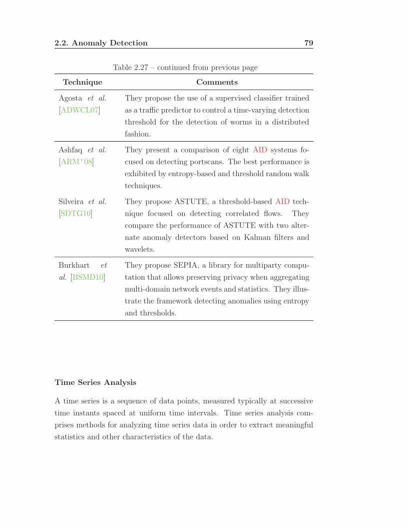
2.2. Anomaly Detection 79
Table 2.27 – continued from previous page
Technique Comments
Agosta et al.
[ADWCL07]
They propose the use of a supervised classifier trained
as a traffic predictor to control a time-varying detection
threshold for the detection of worms in a distributed
fashion.
Ashfaq et al.
[ARM+08]
They present a comparison of eight AID systems fo-
cused on detecting portscans. The best performance is
exhibited by entropy-based and threshold random walk
techniques.
Silveira et al.
[SDTG10]
They propose ASTUTE, a threshold-based AID tech-
nique focused on detecting correlated flows. They
compare the performance of ASTUTE with two alter-
nate anomaly detectors based on Kalman filters and
wavelets.
Burkhart et
al. [BSMD10]
They propose SEPIA, a library for multiparty compu-
tation that allows preserving privacy when aggregating
multi-domain network events and statistics. They illus-
trate the framework detecting anomalies using entropy
and thresholds.
Time Series Analysis
A time series is a sequence of data points, measured typically at successive
time instants spaced at uniform time intervals. Time series analysis com-
prises methods for analyzing time series data in order to extract meaningful
statistics and other characteristics of the data.

80 Chapter 2. State of the Art
Change Detection Change Detection (CD) is a statistical analysis tool
that tries to identify changes in the probability distribution of a stochas-
tic process or time series. In general the problem concerns both detecting
whether or not a change has occurred, or whether several changes might have
occurred, and identifying the times of any such changes. AID techniques
based on CD assume that any change in the modeled process is related with
an anomaly. In Chapter 3 we present an example of a CD technique to detect
sustained changes in large-scale networks.
Table 2.28 summarizes different approaches to AID based on change de-
tection.
Table 2.28: Change detection based approaches to AID.
Technique Comments
Choi et al.
[CPZ02]
They present a method to detect change points in net-
work traffic volume by detecting non-stationarities.
Cabrera et al.
[CLQ+02]
The authors propose the detection of DDoS attacks by
modeling the rate of change of key MIBs variables.
Thottan and
Ji [TJ03]
They present a method to detect anomalies based on
statistical signal processing technique based on abrupt
change detection.
Schweller et
al. [SGPC04]
They present a method to detect change points based
on sketches (reverse hashing).
Siris and
Papagalou
[SP06]
They present two algorithms to detect anomalies,
specifically SYN flooding DoS attacks. The pro-
posed algorithms are based on threshold and CUSUM
[Pag54].
Chen and
Hwang
[CH06]
They present a method to detect DDoS attacks by us-
ing change aggregation trees at each router.
Continued on next page

2.2. Anomaly Detection 81
Table 2.28 – continued from previous page
Technique Comments
Tartakovsky
et al.
[TRBK06a]
They present three methods to detect anomalies based
on CUSUM and applied to detect TCP SYN flooding
attacks.
Zuraniewski
and Rincon
[ZR06]
They propose two methods for detecting change points
in the network traffic fractality. The first one is based
on a cumulated sum (CUSUM) technique while the sec-
ond uses the Schwarz Information Criterion.
Tartakovsky
et al.
[TRBK06b]
They present two CD methods to detect anomalies.
The methods differ in the training step, and are applied
to network traffic.
Scherrer et al.
[SLO+07]
They present a model for Internet traffic at different ag-
gregation levels using a non-Gaussian process. Based
on such model, they present a method to detect anoma-
lies based on change detection on the parameters of the
model.
Dewaele et al.
[DFB+07]
They present a method to detect anomalies at a sin-
gle point in the network. To that end, sketches are
used to condense the information on similar groups.
Then, each group is modeled with a multiresolution
non-Gaussian process that is used to detect the anoma-
lies.
Chen et al.
[CHK07]
They present an architecture to detect DDoS attacks
using CD in the traffic volumes of different routers.
Schweller et
al. [SLC+07]
They propose the detection of volume-based anoma-
lies through change detection, using prediction and re-
versible sketches.
Continued on next page

82 Chapter 2. State of the Art
Table 2.28 – continued from previous page
Technique Comments
Rebahi et al.
[RSM08]
They present a CD method to detect attacks against
IP multimedia subsystems based on CUSUM.
D’Alconzo
et al.
[DCRM10]
They present a method to detect anomalies on 3G mo-
bile traffic. The method is based on detecting changes
on traffic distributions.
Mandjes and
Zuraniewski
[MZ11]
They propose the use of CUSUM-type change point
detection techniques for detecting overload periods in
network links in a setting in which each connection
roughly consumes the same amount of bandwidth.
Forecasting Time Series Forecasting (TSF) is the use of a model to predict
future values based on previously observed values. Typically, the predicted
values are given along with a confidence interval. Consequently, the AID
techniques based on TSF flag as anomalous any data instance that lie outside
the confidence interval provided on their prediction. In this section we can
also include regression models, where the residuals for the test instances are
used to provide anomaly scores. In Chapter 4 we provide an example of a
TSF technique for the detection of anomalies in Voice over IP (VoIP) call
count data.
Table 2.29 summarizes different approaches to AID based on forecasting.

2.2. Anomaly Detection 83
Table 2.29: Forecasting approaches to AID.
Technique Comments
Brutlag
[Bru00]
The author propose a method to detect aberrant be-
havior using the Holt-Winters prediction method.
Eskin et al.
[ELS01]
They present the use of dynamic windows in the de-
tection of system-call anomalies. They use prediction
to detect whether a sequence is probable or not.
Balajinath
and Ragha-
van [BR01]
They use genetic algorithms to learn the individual
user behavior and detect anomalies by predicting cur-
rent user behavior based on past observations.
Dagon et al.
[DQG+04]
They present a method to detect worms by using hon-
eypots (§ 2.2.5). They use logit regression to detect
clusters of relevant events.
Ye et al.
[YCB04]
They present two models for forecasting system calls
and detect anomalies when the χ2 distance to the pre-
diction is high.
Kang et al.
[KFH05]
They present a new model for representing system calls
and test its efficiency when applied to AID.
Zhang et al.
[ZGGR05]
They introduce the term anomography, which is the
union of anomaly detection using tomographic data.
They present and compare different techniques.
Schweller et
al. [SLC+07]
They propose the detection of volume-based anoma-
lies through change detection, using prediction and re-
versible sketches.
Continued on next page

84 Chapter 2. State of the Art
Table 2.29 – continued from previous page
Technique Comments
Agosta et al.
[ADWCL07]
They propose the use of a supervised classifier trained
as a traffic predictor to control a time-varying detection
threshold for the detection of worms in a distributed
fashion.
Lu and Ghor-
bani [LG09]
They propose an AID system using wavelets and Gaus-
sian mixture models. They define 15 network features
that are able to model the normal network situation.
The, using wavelets and an autoregressive model they
fit the time series of the characteristics. The residuals
of the regression are used to detect the anomalies.
Silveira et al.
[SDTG10]
They propose ASTUTE, a threshold-based AID tech-
nique focused on detecting correlated flows. They
compare the performance of ASTUTE with two alter-
nate anomaly detectors based on Kalman filters and
wavelets.
2.2.4 Problems of Anomaly Intrusion Detection
The application and development of AID systems is problematic in many
ways. First, the evaluation of new proposed AID systems lacks of properly
labeled data. This situation also obstruct the comparison of different AID
systems in order to select the system which better fits the needs of the man-
ager. Second, current network monitoring approaches are based on sampling
to cope with the ever-increasing communication speeds. This entails a infor-
mation reduction that may spoil the AID techniques applied in current IDSs.
However, despite of the traffic sampling, the amount of data to be analyzed
by an IDS is humongous, and usually is high-dimensional. Working with such

2.2. Anomaly Detection 85
large datasets make the training and testing phases of AID systems very time
consuming, and it may even prevent some AID systems to be deployed in
an on-line fashion. Moreover, the presence of none-relevant features in such
data sets may also reduce the detection accuracy of some AID systems. Con-
sequently, feature selection has gained interest in the recent years in order
to work only with the most relevant features to detect the target intrusions.
Finally, the fact that AID systems place large number of false alarms is vox
populi. Such large number of false positives is the reason for the limited
deployment of AID systems in real networks under production, because the
network manager has to manually inspect all the raised alarms in order to
filter those that were not related with a security compromise, and automated
responses to detected attacks cannot be applied, because they may lead to
self-imposed denials of service. We further analyze these problems related
with AID in what follows.
Evaluation of IDSs
Evaluating IDSs requires that the datasets used for testing have properly
labeled the data instances as normal or anomalous. This is also a require-
ment for the training datasets in supervised learning techniques. However,
labeling audit data is a very challenging and time consuming task. Such dif-
ficulty is observed by the scarce availability of free datasets for testing IDSs.
The most popular, and almost the only, labeled datasets for evaluating IDSs
were provided by the Lincoln Laboratory at MIT under the DARPA sponsor-
ship. Such laboratory provided two datasets ([LFG+00] and [LHF+00]) for
off-line evaluation of IDSs, but the process was discontinued, mainly because
of the mentioned difficulties in generating such datasets. The datasets were
generated in a controlled private network, with a mix of real and simulated
machines using custom software automata that generated background traffic,
while the 32 different attack types were targeted to the real machines. There
were four different sources for the datasets: sniffed network traffic, Solaris
Basic Security Mode (BSM) audit data, Windows NT audit data (added
in [LHF+00]), and file-system snapshots; and two datasets were provided

86 Chapter 2. State of the Art
for evaluation, one with labeled attacks for training purposes, and an unla-
beled one for fairly testing the different AID approaches. Later, Stolfo et
al. extracted basic features and derived secondary features from these origi-
nal data and created the KDD Cup 1999 data2 that was used for the Third
International Knowledge Discovery and Data Mining Tools competition.
However, despite the impressive undertaking of the Lincoln Lab evalua-
tion program, it has raised criticism regarding the methodologies used in the
evaluation and the generation of the datasets [McH00]. McHugh stressed the
lack of documentation of the experimental approach and the relative poor
basis for characterizing IDSs that the measures used in the evaluation pro-
vide. Such measures were the operating points of the different algorithms
tested. Receiver Operating Characteristic (ROC) techniques analyze the
trade-off between false alarm and detection rate for detection systems, and
were originally developed in the field of signal detection. McHugh criticizes
that ROC analysis is not a constructive measure, claim raised by some of the
participants in the evaluation as well. This has motivated the development
of more specific measures for evaluating IDSs. For instance, Cardenas et
al. [CBS06] propose Intrusion Detection Operating Characteristic (IDOC)
curves as a new IDS performance trade-off which combines in an intuitive
way the variables that are more relevant to the ID evaluation process. Ring-
berg et al. [RRR08] present the basic needs for evaluating AID systems,
claiming that the field deserves more rigor and an universal framework that
permits performance comparisons. They propose to use anomaly simula-
tion and background traffic in addition to labeled datasets to enhance IDSs
evaluation.
Finally, despite of the shortcomings pointed out by McHugh, there is a
large amount of research on IDSs that have used the DARPA datasets to
evaluate their proposals. We would like to note that these datasets are too
old for being useful for evaluation, and comparing the performance of new
developed techniques for AID with those evaluated in DARPA competitions
is extremely unfair.
2The dataset is available at http://kdd.ics.uci.edu/databases/kddcup99/
kddcup99.html

2.2. Anomaly Detection 87
Sampling
With the ever-increasing speeds of communication channels, sampling is a
must rather than an option in network traffic measurement. Sampling pro-
cedures are applied in several monitoring systems, such as NetFlow, and ba-
sically selects individuals (e.g., packets, flows, etc.) from within a population
(i.e., the network traffic) to estimate characteristics of the whole population
when observing the whole population is infeasible. However, despite of its
necessity, there have been several works pointing out the drawbacks that
sampling entails for AID ([BTW+06, MCS+06, MSC+06]).
These works have evaluated the impact of sampling on anomaly detection
metrics and whether sampled data is sufficient for anomaly detection. The
authors of [BTW+06] have observed that simple random sampling, which
is the most typically applied sampling technique, does not severely affect
the distributions of the number of bytes and packets, whereas the sampled
flow distribution significantly differs from the population counterpart. As
a consequence, the AID approaches leveraging on the amount of bytes or
packets work almost perfectly on sampled data, but flow-based AID tech-
niques [SSS+10] experience a decrement in their performance. Furthermore,
they found out that sampling affect the most the volume-based techniques,
whereas entropy-based alternatives maintain almost all their properties un-
altered, thus recommending their use when using sampled data.
There exist other sampling methods proposed in the literature, and some
of them are evaluated by Mai et al. [MCS+06]. Specifically, they compare
the simple random sampling with smart sampling [DLT03], flow-sampling
[DLT04] and sample-and-hold [EV03]. Among these techniques, the best
performance is observed with flow-sampling because it maintain higher accu-
racy at the flow level. On the other hand, smart sampling and sample-and-
hold are focused on detecting large flows (heavy-hitters), which makes them
irrelevant for AID because AID techniques focus typically on small flows.
To solve the problems that come along with sampling network traffic, An-
droulidakis et al. [ACP09] present an study on how network traffic sampling
may be improved in order that not only the impact of the sampling process

88 Chapter 2. State of the Art
on AID techniques is reduced, but also AID gets improved after the sampling
process. To this end, they propose selective sampling, that is able to remove
not interesting network data by opportunistically and preferentially sampling
traffic data with the aim of achieving a magnification of the appearance of
anomalies within the sampled data set.
Feature Selection and Reduction
Reducing the number of features used in an AID system reduces the training
and detection times. This is very advantageous, specifically reducing the
detection times, as it enable the deployment of the AID system to work in an
on-line fashion. Consequently, selecting an appropriate number of features on
which the AID approach is designed enhances the detection system, and may
also improve the system’s performance in a similar way that does selective
sampling [ACP09].
The problem of feature selection is of paramount importance in genetics,
where the number of features is overwhelming. It focuses on removing ir-
relevant features (those that not contribute to differentiate the instances in
the classification problem) and redundant features (those whose information
is contained or can be derived from other features). Many feature selection
techniques have been developed, and the interested reader is referred to the
survey of Chen et al. [CLCG06] for a detailed review of the state of the art.
An alternative to feature selection is feature transformation. Examples
of feature transformation are singular value decomposition and PCA, which
is one of the reasons for this technique being so popular for AID (see Sec-
tion 2.2.3).
False Positives
Current AID systems are popular for placing large number of false alarms.
Such false alarms appear as a result of the lack of interpretation of the dis-
covered suspicious events—an AID system classify audit data as normal or
anomalous, but do not provide detailed information regarding the nature of
the abnormality. False positives reduce the performance of AID system for

2.2. Anomaly Detection 89
several reasons. First of all, there is a very high cost of errors, specially
when compared to other fields where anomaly detection is applied [SP10].
A false positive forces the manager to spend time examining the reported
incident to ensure that the flagged event is malicious, discovering eventually
that it is benign. On the other hand, false negatives entail a compromise of
the monitored system, which may cause serious damage to an organization.
Furthermore, the high number of false positives prevent AID systems to take
automated response to the discovered events. Blocking an attack by dy-
namically reconfiguring a firewall to drop packets from the intruder-flagged
connection may result in an undesired denial of service to a benign user if it
is done in response to a legal network action wrongly identified as an attack.
For this reason, there have been studies to reduce the number of false
positives. Noel et al. [NWY02] propose a framework to characterize ID
activities: degree of attack guilt. This framework allows to assign a con-
fidence score to reported alarms and share such scores in order to reduce
the false positives rate. Kruegel et al. [KMRV03] identified two reasons for
the large number of false alarms, namely the simplistic aggregation of model
outputs in the decision phase and the lack of integration of additional infor-
mation into the decision process, and proposed an event classification scheme
to mitigate such shortcomings. The event classification scheme is based on
Bayesian networks, which improve the aggregation of different model outputs
and the incorporation of additional information. Their experimental results
show that the accuracy of the event classification process is significantly im-
proved. Later, Axelsson [Axe04] proposed to use a visualization process to
interact with the training of a Bayesian classifier, in order to reduce the false
positives rate by adjusting the model parameters. More recently, Gil Perez
et al. [GPGMMPSG12] proposed to assign a reputation score to each IDS
within a network, where the different IDSs collaborate to detect distributed
attacks. The reputation score is used to discard alarms from low reputation
IDSs, thus lowering the number of false alarms. Such reputation score is
based on previous interactions and alerts placed by each IDS.

90 Chapter 2. State of the Art
2.2.5 Future Trends in Anomaly Intrusion Detection
Future trends in AID have to focus on solving the problems pointed out in
the previous section, principally those related with evaluation of IDSs and
reduction of false positives rate. Regarding the former, more effort is needed
to develop ground-truth datasets, where the behavior-deviating patterns are
properly labeled and hence practitioners may evaluate their proposals to
be aware of their shortcomings. In addition, a fair comparison metric for
comparing different AID solutions is still missing. Those metrics proposed as
alternative to ROC analysis lack of generality, as the parameters values they
use (such as the cost associated with false positives/negatives) are system
dependent.
Regarding the false positives rate, we believe that reducing it is the main
open challenge in AID. One intermediate step could be the reduction of man-
ager’s analysis time spent in checking the reported alarms. To accomplish
such time reduction, we propose to use clustering techniques in order to
inspect groups of alarms instead of reviewing them individually. If an ap-
propriate clustering is obtained, then the manager would be able to inspect
only several alarms from a cluster in order to decide whether a given alarm
cluster constitutes a real threat or is a false alarm, thus saving great amount
of expensive manager time.
Another field of further investigation is to find ways to keep pace with cur-
rent networks’ increased size, speed, and dynamics. Paxson et al. [PAD+06]
propose to rethink hardware support for network analysis and ID. In this
light, the use of Graphic Processing Unit (GPU) acceleration to design high-
performance software, such as PacketShader [HJPM10] (a software router
framework for general packet processing with GPU acceleration) may open
new avenues for improving AID systems’ performance.
We would also like to note that, after the exhaustive revision of the lit-
erature provided, we have observed that the number of spatial-based AID
systems is surprisingly scarce. It is our belief that spatial-based AID systems
would gain interest by practitioners given the benefits that such approaches
may imply for the management of large-scale networks. Spatial analysis of

2.2. Anomaly Detection 91
the anomalies may in addition detect different kinds of attacks that go un-
noticed when observed at a single network point, by taking into account
correlations of the observed values at different network points and not only
its marginal distributions.
Finally, we believe that there is still a large gap to fill in the intrusion
security area based on detection of anomalies in order to be deployed in
real systems under production. Current approaches are based on hybrid
system, where a misuse intrusion detection components are used to detect
well-known attacks at high detection rates with the support of AID compo-
nents to quarantine unknown kind of attacks. Such systems would benefit
the usage of HPs in addition. A Honeypot (HP) is a trap set to detect,
deflect, or in some manner counteract attempts of unauthorized use of in-
formation systems. Generally it consists of a computer, data, or a network
site that appears to be part of a real network, but is actually isolated and
monitored, and which seems to contain information or a resource of value to
attackers. Consequently, any connection attempt to the HP is highly prob-
able of being a malicious activity. In this way, HPs may be regarded as a
surveillance system using cameras that record the intruder when trying to
open a safeguard that allow observing the intruder’s techniques to evade the
systems security. Furthermore, HPs will keep the attacker busy leaving more
time for the system manager to take response, and, as a consequence, HPs
may waste attackers’ time and force them to gave up promptly after failing
to reach their objectives.
2.2.6 Conclusions
This section presented a survey of the state of the art of anomaly intrusion
detection, focusing on the period 2000-2012. During this period, numerous
studies have presented research in new ways of discovering abnormal events
using network or host data. We believe this is the more comprehensive survey
on AID systems to date. We have presented in addition a survey of the
proposed taxonomies to classify the existing AID techniques, and proposed
a new comprehensive one. The taxonomy allowed us to present the main

92 Chapter 2. State of the Art
techniques applied in AID in an structured manner.
Furthermore, we have analyzed the main problems affecting the AID
paradigm, and which future trends should be addressed in order to solve
them. We hope that this work can serve as a useful guide through the maze
of the literature, enabling the understanding of the different approaches to
allow new practitioners focusing on the AID techniques that are prone to
provide higher performance given their specific requirements.
Chapter 3
Detection of Traffic Changes in
Large-Scale Backbone
Networks
Network management systems produce a huge amount of data in large-scale
networks. For example, the Spanish academic network features hundreds of
access and backbone links, each of which produces a link utilization time se-
ries. For the purpose of detecting relevant changes in traffic load a visual
inspection of all such time series is required. As a result, the operational ex-
penditure increases. In this chapter, we present an on-line change detection
algorithm to identify the relevant change points in link utilization, which are
presented to the network manager through a graphical user interface. Conse-
quently, the network manager only inspects those links that show a stationary
and statistically significant change in the link load. These changes may call
for link’s capacity upgrade in order to maintain desired levels of Quality of
Service.
3.1 Introduction
In large-scale networks, the amount of information provided by management
systems is huge. For example, time series of traffic volume or network link
93

94Chapter 3. Detection of Traffic Changes in Large-Scale Backbone
Networks
load may be provided per each access link. Network managers face with
visual inspection of far too many graphs, which motivates automated proce-
dures that basically pinpoint which are the links that deviate from a typical
behavior and demand intervention from the manager, out of the many links
present in the network. We propose a load model for network links that is
capable of efficiently tracking sustained load changes in network links. These
sustained changes may call for link’s capacity upgrade in order to maintain
a desired level of Quality of Service (QoS). Our model is suitable for any
network link with high aggregation—e.g., backbone links and access links
of large institutions. It is aimed at facilitating network-wide monitoring of
large-scale networks, by clearly identifying network links with a varying traf-
fic behavior. Moreover, forensic data for each link can be later analyzed
off-line, in order to spot possible correlations that serve to understand how
the detected load changes in one link have impacted the performance of the
rest of the network.
Previous approaches to network-wide traffic analysis use point-to-point
[BDTJ02, LPC+04] or point-to-multipoint [FGL+01] models for analyzing
the demands in backbone networks. The key concept in these works is the
Origin-Destination (OD) flow. An OD flow is a time series that comprises
all the traffic that enters the backbone in a given Point of Presence (PoP)
and leaves in another PoP. Therefore, the analysis of the backbone demands
is divided into n2 time series, each representing an OD flow, being n the
number of PoPs in the backbone network. To compute the OD flow time
series, the authors of these works leverage on flow level measurements to find
the amount of traffic entering the network at each PoP and routing informa-
tion measurements to determine the egress point of each measured flow. Our
approach to network-wide traffic analysis reduces the complexity of the afore-
mentioned methodologies leveraging on link time series. Network topologies
in backbone networks are usually far from being a completely meshed topol-
ogy. Thus, the number of links in a backbone network is considerably lower
than the square of the number of nodes. In our case study, the Spanish
academic network RedIRIS1 comprises 18 PoPs and only 30 backbone links.
1http://www.rediris.es/index.php.en

3.1. Introduction 95
Therefore, our network-wide traffic analysis approach accounts for only 60
elements to monitor (because the links are bidirectional), considerably less
than the 182 = 324 different OD flows with the RedIRIS topology. Moreover,
our model is fed only with average load measurements at high granularity
(90 minutes intervals), which can be easily obtained from Simple Network
Management Protocol (SNMP) measurements [Sta98]. This also entails a
complexity reduction compared with the other network-wide traffic analysis
approaches existing in the literature. Our model needs simpler measure-
ments and simpler post-processing steps for the measurements, which makes
it amenable for on-line application and enables its utilization in a broader
set of network links.
We think this work is relevant to network operators and the research
community. On one hand, network operators are aware of the importance of
detection of traffic changes, which are relevant at different timescales. Load
changes at short timescales are relevant for attack detection, where a sudden
change in the load may be related with flash crowds or Denial of Service
(DoS) attacks [BKPR02, CH06, KSZC03, SGPC04]. On the contrary, load
changes at long timescales (in the scale of days or weeks) should be taken into
account for traffic engineering task such as load balancing and capacity plan-
ning in order to guarantee some predefined levels of QoS [PTZD05, FGL+00].
To the best of our knowledge, there is little existing work in the literature
regarding traffic engineering procedures based on the detection of statisti-
cally significant sustained changes, and the more relevant approaches are
normally based on simple time series forecasting techniques [Bru00] focused
on short-term changes. In those cases, a prediction of the load is used to
compute confidence bands, where the actual value of the load should lie in
under normal network performance. However, this methodology is not able
to determine whether the change is stationary (i.e., the changed value is
maintained over several time periods) and therefore the traffic behavior has
changed. Consequently, in practice, the network manager should visually
inspect the different link load plots to make such decision. In contrast, our
methodology focuses only on sustained changes that may imply a shift in
users’ behavior, and the network manager should take action in response to

96Chapter 3. Detection of Traffic Changes in Large-Scale Backbone
Networks
such shift in order to maintain the offered QoS on the network.
In this chapter, we provide techniques that allow the network manager to
focus only on those links that show stationary load changes. The case study
is the Spanish Academic Network RedIRIS. We note that RedIRIS features
30 bidirectional backbone links and hundreds of connections to large insti-
tutions, and it is not feasible to analyze all of the corresponding time series
separately from an Operational Expenditures (OPEX) point of view. Con-
sequently, our proposed technique filters out those links which do not show
statistically significant changes in the traffic behavior. As a result, the OPEX
is largely reduced, because the traffic engineering tasks are only performed on
a reduced subset of links. To identify such changes, we developed an on-line
algorithm that uses clustering techniques and statistically sound method-
ologies to determine the location and statistical significance of the change
points. In addition to providing valuable techniques to discriminate load-
changing links, which have a direct impact in OPEX reduction, our findings
also serve to gain insight about the dynamics of load change in large-scale
networks. Is the load change continuous or showing sudden change in mean?
How frequent are load changes in a large network? Our analysis serves to
address these issues with a dataset that is three-year long and comprises the
whole Spanish academic network—i.e., more than one million users.
Our proposed algorithm is based on a fairly multivariate Gaussian vector
that models the daily traffic pattern of links with large aggregation level.
Such model splits the 24 hour day period into 16 non-overlapping intervals
of 90 minutes starting at midnight, each of which is a vector component. We
have validated our fairly Gaussian model with real network measurements
obtained also from the RedIRIS network, showing evidence that the signifi-
cance of the normal theory tests of mean vectors and covariance matrices is
not severely affected by the deviations from normality existing in actual data.
This result allows us to apply multivariate normal inference to the mean vec-
tor, namely the Multivariate Behrens-Fisher Problem (MBFP) procedure, to
determine if there is a statistically significant difference in the mean vectors
of two consecutive time series. Therefore, when there is evidence of a change
in the load time series, we alert the network managers, allowing them to take

3.1. Introduction 97
the appropriate action as a response to that change.
After assessing the performance of the load change detection algorithm,
we have applied it to such real network measurements, showing the efficiency
in reducing the number of times the network needs supervision. We have
analyzed more than 300 days worth of data, and in average, we have placed
around 11 alerts per link. This supposes that a network manager would have
receive an alert for a statistically significant and sustained change less than
4% of the days. In the remaining days, the network is considered stable and
no action is required.
A distinguishing feature of the MBFP procedure to detect changes is that
it evaluates the difference in the mean vectors taking all the vector compo-
nents into account at the same time. This may result in changes that are due
to either small differences in several vector components or large differences in
a single vector component. In addition, as the vector components represent
time intervals, the relevance of a change may be different depending on the
vector component that caused the change detection. For instance, changes
at night-time may not be relevant compared to those at the busy hours.
Consequently, we devise an alert color code to categorize the change points
located by our algorithm. Such color code is used to create weather maps
of the network, allowing to visually inspect the relevant events happening in
the network in an straightforward manner.
The rest of the chapter is organized as follows: Section 3.2 is devoted to
present the measurement dataset. Section 3.3 describes the load model and
presents the methodology and results of its validation process. Section 3.4
presents the on-line load change detection algorithm and the assessment of
its performance with synthetic data. Section 3.5 provides the results of the
application of the algorithm to actual network measurements and Section 3.6
shows how the proposed methodology could be applied to monitor a large-
scale network like RedIRIS. Finally, Section 3.7 concludes the chapter.

98Chapter 3. Detection of Traffic Changes in Large-Scale Backbone
Networks
3.2 Measurement Dataset
This section is devoted to present an overview of the network traffic mea-
surements used in this chapter. As we noted in the previous section, our
algorithm is fed by average load measurements computed at non-overlapping
intervals of 90 minutes length. A simple averaging process of SNMP measure-
ments obtained at 5 minutes granularity is enough to obtain such data. We
gather network measurements at such resolution from Multi Router Traffic
Grapher (MRTG) tools [OR98] installed on the network equipments of the
Spanish academic network RedIRIS (see Section 2.1.3 for a detailed descrip-
tion of MRTG). In what follows, we present a description of the dataset and
the network from which we obtained such measurements, and an overview
of the daily and weekly traffic patterns that characterize the links in the
network.
3.2.1 Description of the Measurement Dataset
The RedIRIS network comprises 18 PoPs spread along the Spanish country
(Figure 3.1 shows the backbone network topology), and provides Internet
access to more than 350 institutions, mainly universities and public research
centers, which make up a grand total of more than a million users. In addi-
tion, it has several Internet exchange points with the European Research and
Education Network GEANT, and with other ISPs (Telia, Global Crossing,
etc.). RedIRIS provided us with MRTG records and flow summaries of the
PoPs in Figure 3.1 and from an extensive set of universities and exchange
points. We have selected 18 links out of the total to make this study, which
transport large amounts of data and are representative of the variety of links
that are present in the network. Our dataset includes 10 university links, 5
backbone links of the RedIRIS core network and 3 links that provide con-
nection with exchange points or the European academic network GEANT2.
For privacy concerns, we label the University links as U1, U2, . . . , U10. We do
the same with the Backbone links, B1, B2, . . . , B5, and the eXchange point
2http://www.geant.net/

3.2. Measurement Dataset 99
links, X1, X2 and X3.
����������
�����
��������������
Figure 3.1: RedIRIS network architecture.
In total, we have collected and analyzed three-years worth of MRTG
records (2007, 2008 and 2009). MRTG have been configured with measure-
ment intervals of 5 minutes—i.e., there is a new record every five minutes.
With this time granularity, we have 288 records for each day and direction
(incoming/outgoing) in every link. Our measurements span from the 2nd of
February 2007 to the 10th of March 2009, namely we collect more than 750
days worth of data per link. Such MRTG records contain five different fields:
the UNIX timestamp of the measurements (which will play an special role in
the measurements preprocessing step) and the average and maximum trans-
fer rates, in bps, for both interfaces in the last measurement interval. We
summarize some relevant information about the links present in the dataset
in Table 3.1.
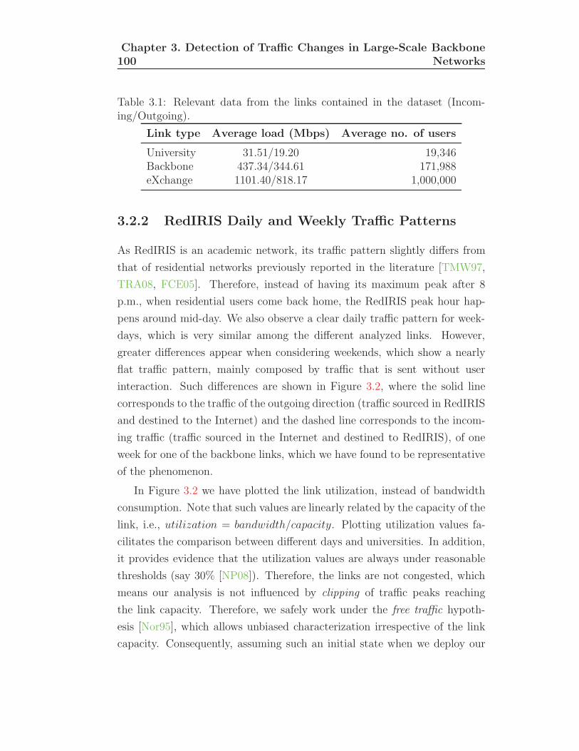
100Chapter 3. Detection of Traffic Changes in Large-Scale Backbone
Networks
Table 3.1: Relevant data from the links contained in the dataset (Incom-ing/Outgoing).
Link type Average load (Mbps) Average no. of users
University 31.51/19.20 19,346Backbone 437.34/344.61 171,988eXchange 1101.40/818.17 1,000,000
3.2.2 RedIRIS Daily and Weekly Traffic Patterns
As RedIRIS is an academic network, its traffic pattern slightly differs from
that of residential networks previously reported in the literature [TMW97,
TRA08, FCE05]. Therefore, instead of having its maximum peak after 8
p.m., when residential users come back home, the RedIRIS peak hour hap-
pens around mid-day. We also observe a clear daily traffic pattern for week-
days, which is very similar among the different analyzed links. However,
greater differences appear when considering weekends, which show a nearly
flat traffic pattern, mainly composed by traffic that is sent without user
interaction. Such differences are shown in Figure 3.2, where the solid line
corresponds to the traffic of the outgoing direction (traffic sourced in RedIRIS
and destined to the Internet) and the dashed line corresponds to the incom-
ing traffic (traffic sourced in the Internet and destined to RedIRIS), of one
week for one of the backbone links, which we have found to be representative
of the phenomenon.
In Figure 3.2 we have plotted the link utilization, instead of bandwidth
consumption. Note that such values are linearly related by the capacity of the
link, i.e., utilization = bandwidth/capacity. Plotting utilization values fa-
cilitates the comparison between different days and universities. In addition,
it provides evidence that the utilization values are always under reasonable
thresholds (say 30% [NP08]). Therefore, the links are not congested, which
means our analysis is not influenced by clipping of traffic peaks reaching
the link capacity. Therefore, we safely work under the free traffic hypoth-
esis [Nor95], which allows unbiased characterization irrespective of the link
capacity. Consequently, assuming such an initial state when we deploy our

3.3. Multivariate Normal Model for DailyTraffic 101
Monday Tuesday Wednesday Thursday Friday Saturday Sunday0
0.02
0.04
0.06
0.08
0.1
0.12
0.14
0.16
Day of the week
Util
izat
ion
(dim
ensi
onle
ss)
Incoming trafficOutgoing traffic
Figure 3.2: Time Series representation of the utilization of a RedIRIS linkfor a whole week.
proposed methodology in a network and that the manager takes into consid-
eration the alerts placed by the algorithm, the network should not present
saturation during long periods of time and the free traffic hypothesis should
remain valid.
3.3 Multivariate Normal Model for Daily
Traffic
In this section, we present our multivariate model for network daily traffic
load, and show practical evidence of its applicability. We assume that the
network measurements to model come from SNMP reports at 5 minutes
granularity due to its popularity, or instead come from another measurement
methodology but using the same format. This model takes advantage of
the apparently invariance of the daily traffic pattern shape for working days
presented in Section 3.2.2. The methodology for the model validation is
presented in Section 3.3.2, and the corresponding results can be found in
Section 3.3.3. Finally, a discussion of the results concludes this section.

102Chapter 3. Detection of Traffic Changes in Large-Scale Backbone
Networks
3.3.1 Description of the Multivariate Normal Model
From the overview of the RedIRIS daily traffic pattern, we can clearly differ-
entiate between weekdays and weekends. The former have a clear day-night
pattern, which is influenced by the number of users being active (sending
or receiving traffic) at the different times of the day. On the contrary, the
weekends have a nearly flat, less utilized daily pattern, which supports the
hypothesis that such traffic is mainly due to standalone applications, with
no user interaction. Accordingly, we remove weekends, summer & Christmas
holidays, national & regional holidays and eventually examination periods.
Thus, we only consider working days, which are more interesting for traffic
engineering purposes.
The model assumes that measurements of the same interval during dif-
ferent days come from the same (at first hand unknown) probability distri-
bution. We base such an assumption in the fact that the shape of the traffic
pattern does not show significant variation with time. Consequently, the
differences between the measurements in the same measurement interval of
different days should be small (if there is no change in the users’ behavior).
However, such probability distribution does not have the same parameters
between different measurement intervals of the same day, for instance at 12:00
a.m. and at 12:00 p.m. Therefore, a multivariate distribution to model the
daily network load seems to be reasonable, with each measurement interval
having its own parameters.
However, the number of different measurement intervals per day with the
default SNMP time granularity of the reports (5 minutes, which results in
288 measurements per day) is too large. Actually, a 288-variate model is
not analytically tractable [Don00]. In order to make the model more man-
ageable, we averaged the load values into 16 disjoint intervals of 90 minutes
(i.e., we average 90/5 = 18 SNMP samples to form each of the vector com-
ponents). The reasons to choose such averaging period are manifold: first,
we need the averaging period to be a multiple of the measurement gran-
ularity and a divisor of the number of minutes in a day; second, chances
are that data are missing in the five minutes timescale, but having 18 con-

3.3. Multivariate Normal Model for DailyTraffic 103
secutive five-minutes interval samples missing is unlikely. Note that if all
measurements from an averaging interval are missing, we place an alert to
the network manager (the link may be down), and then remove the whole
day from the sample, because the Gaussian vector is incomplete3; third, the
different measurement points may not be synchronized. A timescale of 90
minutes is coarse enough to circumvent this problem, as stated in [PTZD05];
fourth, the averaging process reduce the bias that outliers and measurement
errors introduce to the results; last, but not the least, the assumption of fairly
Gaussian Internet traffic holds when there is enough temporal aggregation
of the measurements [KN02, vdMMP06, vdBMvdM+06]. Consequently, in
addition to simplifying the model, we obtain a reasonable distribution for the
averaged samples (however, we take the fairly normal distribution only as an
hypothesis, and show practical evidence of the validity of such assumption
in the remaining of the section).
After the preprocessing step, which removes the holidays and incomplete
day-vectors, the dataset contains more than 300 samples per link and direc-
tion, each of them representing a day worth of traffic data that we model
with a 16-variate Gaussian distribution. Note that this preprocessing step
can be done in an on-line fashion, because the days to be removed are known
in advance. Finally, Figure 3.3 shows the time series of the average daily
utilization pattern of the RedIRIS network with the 16 selected intervals
presented in Table 3.2.
To summarize, we present the assumptions relevant to the model in the
following bullet list:
• The daily traffic-pattern shape can be regarded as short-term invariant.
• The utilization of the links is always below critical levels, e.g., 60%.
That means that we safely work under the free traffic hypothesis.
• Measurements from the same interval during different days come from
the same probability distribution.
3Alternatively, the network manager could decide to apply missing value techniquessuch as replacing with the mean value of such vector component of the cluster [AH08,Chapter 13].

104Chapter 3. Detection of Traffic Changes in Large-Scale Backbone
Networks
0 5 10 15 200
0.1
0.2
0.3
0.4
Hour of the day
Util
izat
ion
(dim
ensi
onle
ss)
RedIRIS daily traffic pattern
Figure 3.3: Time Series representation of the average utilization pattern ofthe RedIRIS network (solid line) and time divisions according to the multi-variate model (vertical dashed lines).
Table 3.2: Correspondence between vector components and time of day.
VectorTime interval
VectorTime interval
component component
1 00:00-01:30 9 12:00-13:302 01:30-03:00 10 13:30-15:003 03:00-04:30 11 15:00-16:304 04:30-06:00 12 16:30-18:005 06:00-07:30 13 18:00-19:306 07:30-09:00 14 19:30-21:007 09:00-10:30 15 21:00-22:308 10:30-12:00 16 22:30-00:00

3.3. Multivariate Normal Model for DailyTraffic 105
• The parameters of such distribution depend on the actual interval of
measurement.
• The Gaussian distribution is appropriate for modeling the average load
in such intervals (this assumption is validated in Section 3.3.3).
3.3.2 Methodology
To validate the applicability of the model to network traffic inferences, we
have performed several verifications of the fairly Gaussian assumption. More
specifically, we have adopted the methodology used in [vdMMP06] to verify
the fair normality of the marginal distributions of our multivariate model. In
addition to this, we have also tested for Multivariate Normality (MVN). This
is necessary because the fact that several variables have univariate normal dis-
tributions does not imply that they jointly have normal distribution [Kow73].
In what follows, we briefly describe the normality tests applied for both uni-
variate marginal and the joint multivariate distributions.
Van de Meent et al. [vdMMP06] have shown that the linear correlation
coefficient γ between the order statistics of the sample and the corresponding
normal quantiles of the model distribution (i.e., a normal distribution with
parameters estimated from the sample) is, roughly speaking, equivalent to
the Kolmogorov-Smirnov (KS) test for testing univariate normality, i.e., if
γ > 0.9, then the null hypothesis of normality cannot be rejected by the KS
test at significance level 0.05 (see Appendix A for further description of the
KS test). We have followed such approach and calculated the coefficient γ
for each of the 16 univariate normal distributions according to our model. To
compute γ, let x1, x2, . . . , xn be a univariate sample of size n. Let x and s2
be the unbiased estimates for the sample mean and the sample variance, i.e.,
x = n−1∑n
i=1 xi and s2 = (n− 1)−1∑n
i=1(xi − x)2. Define x(i), i = 1, 2, . . . , n
as the order statistics of the sample, i.e., x(1) < x(2) < . . . < x(n), and qi their
corresponding quantiles given by qi = Φ−1( in+1
), where Φ−1 is the inverse of
the normal cumulative distribution function with mean x and variance s2.
Denote by q the mean of the quantiles, then the linear correlation coefficient
γ is given by:

106Chapter 3. Detection of Traffic Changes in Large-Scale Backbone
Networks
γ =
∑n
i=1(x(i) − x)(qi − q)√∑n
i=1(x(i) − x)2∑n
i=1(qi − q)2. (3.1)
Regarding MVN, we have selected Mardia’s multivariate skewness and
kurtosis coefficients b1,p and b2,p [Mar70] to measure deviations from MVN.
The main reasons to select these statistics are their affine invariance prop-
erty and tractability. Moreover, Mardia has shown that the significance of
the normal theory tests of mean vectors and covariance matrices is adversely
affected by skewness [Mar75] and kurtosis [Mar74], respectively, i.e., having a
large skewness (kurtosis) deviation from multinormality adversely affects the
false positive rate of normal theory tests applied to the mean vector (covari-
ance matrix). Therefore, we can assess fairly MVN by using these tests and,
in addition, this can shed light on the suitability of our multivariate model for
making inferences about the mean vector and the covariance matrices—the
methodology we apply in Section 3.4 for change detection makes inference
about the mean vector. Let y1,y2, . . . ,yn be a p-dimensional random sample
of size n, then Mardia’s multivariate coefficients for skewness and kurtosis
are given, respectively, by:
b1,p =1
n2
n∑i=1
n∑j=1
r3ij and b2,p =1
n
n∑i=1
r4i , (3.2)
where n > p and
rij = (yi − y)TS−1n (yj − y), r2i = (yi − y)TS−1
n (yi − y), (3.3)
y =1
n
n∑i=1
yi, Sn =1
n
n∑i=1
(yi − y)(yi − y)T , (3.4)
where xT is the transpose vector of x. For convenience of applying ex-
isting statistical tables, the following standardized forms are used in prac-
tice [Mar70]:

3.3. Multivariate Normal Model for DailyTraffic 107
sb1,p =nb1,p6
d→ χ2df , sb2,p =
b2,p − p(p+ 2)(n− 1)/(n+ 1)√8p(p+ 2)/n
d→ N (0, 1),
(3.5)
where df = p(p+1)(p+2)/6 are the degrees of freedom of the χ2 distribution
andd→ means convergence in distribution (n → ∞). Therefore, large values
of b1,p and |b2,p| (because this second test is two-sided) indicate non-MVN.
3.3.3 Results of the Model Validation
To apply the above-mentioned techniques, we have preprocessed the data
set described in Section 3.2.1 according to the restrictions presented in Sec-
tion 3.3.1 (removal of holidays and incomplete day-vectors).
We have then computed the linear correlation coefficient γ using all the
measurement campaign samples in each direction of each link. The results
were very poor, and the univariate normality was rejected for all the marginal
distributions. However, this does not imply that the model is inappropriate,
but that the parameters may be changing with time, i.e., the sample is non-
stationary. In spite of this, we can assume that the traffic is short-term
stationary [GDHA+11], i.e., that the parameters of the underlying distri-
bution remain nearly stable for a short period of time, say 20-30 days, and
accordingly apply the normality tests to subsamples of that size. For this rea-
son, we have divided our sample into subsamples of size n = 20 day-vectors,
which is equivalent to a period of 25-28 natural days—that is because we rule
out holidays. Consequently, we computed the γ coefficient for each subsam-
ple marginal distribution, and the results are shown in Figure 3.4(a), where
we have plotted the cumulative distribution function of the γ value of such
marginal subsamples.
With regard to MVN, it is well-known that if non-normality is indicated
for one or more of the marginals, MVN can be rejected [JW92, p. 133].
Hence, we do not verify MVN neither for the whole dataset nor for those of
the above-mentioned subsamples in which any of the marginal distributions
was deemed non-Gaussian. To properly apply the corresponding standard-

108Chapter 3. Detection of Traffic Changes in Large-Scale Backbone
Networks
0.4 0.5 0.6 0.7 0.8 0.9 10
0.2
0.4
0.6
0.8
1
γ
F(γ)
Incoming direction
Outgoing direction
(a)
600 650 700 750−0.01
0
0.01
0.02
0.03
sb1,p
sb2,
p
Incoming directionOutgoing direction
(b)
Figure 3.4: Normality test results: (a) Univariate normality results. (b)Multivariate normality results.
ized values of the statistics for testing multivariate skewness and kurtosis,
we cannot use the corresponding limiting distributions, because the size of
our samples is small. Therefore, we ran N = 100, 000 Monte Carlo simula-
tions on N independently generated samples Z ∼ Np(0, Ip) of size n = 20 to
estimate the critical values of the standardized forms of the statistics, where
0 is a vector of 16 components all equal to 0, and Ip is the identity matrix
of rank p = 16. These critical values are summarized in Table 3.3 for three
different significance levels.
Table 3.3: Critical values for the statistical tests for multivariate skewnessand kurtosis.
Significance level (α) cvsb1,p
cvsb2,p
lower upper
0.10 695.7828 −0.0040 0.00540.05 708.6464 −0.0046 0.00690.01 732.4614 −0.0054 0.01
In this table, cvsb1,p refers to the critical value for the standardized value
of b1,p. Values of sb1,p larger than cvsb1,p indicate skewness in the sample.
On the other hand, cvsb2,p lower and cvsb2,pupper are the critical values for
the two-tailed test for kurtosis. Values of sb2,p smaller than cvsb2,p lower or
greater than cvsb2,pupper indicate kurtosis in the sample.
We have presented in Figure 3.4(b) the results of the statistical tests when

3.3. Multivariate Normal Model for DailyTraffic 109
applied to our dataset. We show in the x-axis the value of sb1,p whereas in
the y-axis we can find the values of sb2,p. Each subsample is represented by
a ◦ symbol for the incoming direction or by a × symbol for the outgoing
direction. We have represented with straight lines the thresholds given by
the critical values at the significance level α = 0.01. The percentage of
tests indicating rejection of the null hypothesis are presented in Table 3.4,
where we show the results of the Skewness test, the Kurtosis test and the
combination of both.
Table 3.4: Percentage of rejection of the multivariate skewness and kurtosistests.
Direction
Rejection ratio
Skewness test Kurtosis testEither Skewness
or Kurtosis
Incoming 2.80% 4.60% 6.54%Outgoing 5.88% 8.24% 14.12%Both 4.17% 6.25% 9.90%
3.3.4 Discussion of the Results
The results for the univariate normality test shown in Figure 3.4(a) give
evidence that the performance in the incoming and outgoing directions is
nearly the same, as the corresponding lines for each direction are partially
superimposed. In both of them, it can be seen that for more than 80% of
the cases studied, the goodness-of-fit measure γ was above the threshold 0.9.
Such results are close similar to those of [vdMMP06], so we can obtain a
similar conclusion, i.e., the 16-variate traffic load vector components, when
considered separately, can be deemed as fairly Gaussian.
Regarding MVN, Table 3.4 shows that the model fits better to the incom-
ing direction of traffic. This is a consequence of the larger aggregation of the
incoming traffic, as shown in Table 3.1. When taking both directions into
account, Table 3.4 shows that MVN can be rejected for approximately 10% of
the cases. Although we cannot assume that the multivariate model is totally

110Chapter 3. Detection of Traffic Changes in Large-Scale Backbone
Networks
accurate, there is an evidence based on the results that fairly MVN can be ac-
cepted. Moreover, we can see from such results that our model is suitable for
applying multinormality inference to the mean vector (e.g., the MBFP pro-
cedure), because the percentage or rejections for the skewness tests (4.17%)
is small and therefore the significance of the multinormality theory tests for
mean vectors [Mar75] will not be severely affected. The same conclusion can
be drawn by having a look at the percentage of rejections for the kurtosis
tests (6.25%), which in turn evidences that the significance of multinormality
theory tests for covariance matrices [Mar74] will not be affected drastically.
With regards to outstanding peaks or non sustained congestions, e.g.,
flash crowds, that may spoil the normality of the data, we note that the
effect of such undesirable situations is absorbed by the averaging process
applied in the preprocessing step of the model.
All in all, we note that the fair normality assumption cannot be rejected
for the majority of the subpopulations in the univariate case, and the fair
MVN assumption also seems to be correct, so the fair MVN hypothesis of
the proposed model can be accepted.
3.4 On-line Load Change Detection Algorithm
In the validation of the multivariate model we confirmed that the whole
dataset does not follow a normal distribution, whereas small subsamples of
it actually do. This fact suggest that the parameters of the normal distribu-
tion may be changing slowly with time—i.e., short-term stationarity. This
section presents an on-line load change detection algorithm, aimed at identi-
fying changes in traffic loads when monitoring Internet links. Such algorithm
produces an alert when a sustained and statistically significant change has
been detected. Then, the network manager verifies the change and takes ac-
tion if the change is truly relevant. Our algorithm uses a two-step approach
to detect the change points: first, a clustering technique for selecting poten-
tial change points is applied; then a sound statistical methodology is used to
determine whether changes are casual or they define a breakpoint between
stationary regions. Before describing the proposed algorithm in Section 3.4.2,

3.4. On-line Load Change Detection Algorithm 111
we introduce the applied methodology in Section 3.4.1. Then, we validate the
behavior of the algorithm with synthetically generated time series, showing
the results in Section 3.4.3.
3.4.1 Methodology
In this section, we first present the clustering technique that has been adopted
and then provide a brief introduction to the statistical methodology, namely
the Behrens-Fisher problem. The selected clustering algorithm is k -means
[DHS01], which is a two-step iterative algorithm that finds the clusters by
minimizing the sum of the squared distances to a representative, which is
called centroid. The input to the algorithm is the number of clusters k ex-
isting in the dataset—in our algorithm we always look for two clusters. The
choice of k -means for our on-line algorithm is due to the ease of adding a
new instance to an existing model. To do so, it is only necessary to compute
the distance from the new instance to the existing centroids, and then re-
compute the centroid for the cluster the new instance is assigned to. Finally,
if the centroids have changed, k -means is applied again from a quasi-optimal
solution, so the algorithm finds the new centroids faster than the first time.
On the other hand, in order to obtain clusters that are adjacent in time
(i.e., all samples of the cluster being sequential in time and not out of order),
the UNIX initial timestamp of the last sample of the day is included as an
additional vector component.
In order to verify that the obtained clusters are actually different, we
have applied the MBFP. The MBFP is the statistical problem of testing
whether the mean vectors of two multivariate Gaussian distributed popula-
tions (X(1),X(2)) are the same (null hypothesis H0), for the case of unknown
covariance matrices. Assuming homogeneity of the covariance matrices would
allow applying simpler models, such as MANOVA. However, the homogeneity
of covariance matrices is a strong assumption that indeed is not verified by
the data. This motivates the application of the MBFP whose sole assump-
tions are that X(i) ∼ Np(μ(i),Σ(i)), i = 1, 2; i.e., the samples of population i
come from a p-variate normal distribution with mean vector μ(i) and covari-

112Chapter 3. Detection of Traffic Changes in Large-Scale Backbone
Networks
ance matrix Σ(i). To solve this problem, the Hotelling’s T 2 statistic given
by
T 2 = nYS−1
y YT
n− 1
n− p
p∼ F (3.6)
is used, where Y is a p-dimensional vector Y = (y1, y2, . . . , yp) of the means
of the differences between both populations (X(1),X(2)), assuming both pop-
ulations are of equal size n [And58], and Sy is the unbiased estimation of its
covariance matrix as given by (3.4). This statistic follows a F -distribution
with p and n − p degrees of freedom under H0. However, when the sample
sizes are not the same, a transformation is needed before computing the T 2
statistic [And58, Section 5.6]. The interested reader is referred to Appendix
B.2 for further description of the MBFP procedure. We note that such test
is suitable when using our multivariate model because we have shown, in
Section 3.3, that the skewness of our sample (which is the deviation from
normality that mostly affects hypothesis testing procedures for normal mean
vectors) is typically under the bounds allowed by the statistical test.
The MBFP assumes that the data comes from multivariate normal dis-
tributions. In order to trust in the results of the MBFP test, we have to
make sure that our data is multivariate normal. Although we have assessed
the MVN of our model in the previous section, it was shown that in some
cases such assumption could be rejected. Consequently, we apply the same
analytical tests described in Section 3.3.2 to both clusters before applying
the MBFP. Although it is necessary to test the MVN assumption before
each application of the MBFP test, these tests are lightweight and can be
performed on-line very fast. If the MVN condition does not hold, the dis-
tribution of the T 2 statistic under the null hypothesis may differ from the
central F -distribution, and thus the probability of rejecting the null hypoth-
esis when it is actually true would be different—Type I error. Therefore, we
warn the network manager whenever this happens, in order not to blindly
trust the output of the algorithm.

3.4. On-line Load Change Detection Algorithm 113
3.4.2 Description of the Algorithm
Our on-line load change detection algorithm aims at identifying whether the
detected change point represents a breakpoint between two different station-
ary behaviors of the link load. More specifically, we wish to assess if a change
in the mean vector has occurred. Once detected, the change points are re-
ported to the network managers to let them know that potential anomalies
may have happened. The first step in our algorithm is to preprocess the
measurements in order to obtain daily samples according to the multivariate
model presented in Section 3.3.1.
We do such preprocessing in an on-line fashion, obtaining a day-sample
after all the measurements of a day have been collected, which we add to
the sample set S. When we have enough day-samples (#S ≥ 34), we apply
the k-means technique looking for two clusters. If the reported clusters are
suitable for the algorithm, i.e., each one with at least 17 samples (meaning
two potential sustained change-free regions), we mark as a potential change
point between the reported clusters. Once a potential change point is found,
we apply the MBFP statistical hypothesis testing procedure to the reported
clusters after testing for MVN. Even if the MVN assumption does not hold
(i.e., the MVN tests reject the null hypothesis) the algorithm continues to
the following step, and applies the MBFP test to the populations. However,
the network manager is warned about this fact to be aware of the potential
inaccuracy. Finally, if the MBFP test rejects the null hypothesis of equality
of means, an alert is placed to the network manager that indicates a sustained
and statistically significant change point, and the oldest cluster is removed
from the sample set. The flowchart of Figure 3.5 summarizes the work-flow
of the algorithm.
3.4.3 Validation of the Algorithm
To assess the performance of the load change detection algorithm, we have
tested it with synthetically generated data. Such data allow us to verify
whether the algorithm is detecting the changes properly, because we know
beforehand where the changes are located. The synthetic datasets generated
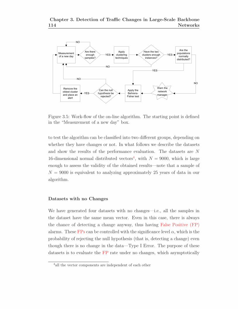
114Chapter 3. Detection of Traffic Changes in Large-Scale Backbone
Networks
����������� � �� ���
��� ���� ����� ��������
��
����� �������� ��������
���� �� �� ������� ����� �������
��
����� �� ������� ����� ��
!"#
$� �� ��� ��������� %� ��&�����
'����� �� ����� ������ �� ����� �
����
!"#
��
!"#
��� �� ��������� �������
�����%����
!"#
(�� �� ����)������
��
Figure 3.5: Work-flow of the on-line algorithm. The starting point is definedin the “Measurement of a new day” box.
to test the algorithm can be classified into two different groups, depending on
whether they have changes or not. In what follows we describe the datasets
and show the results of the performance evaluation. The datasets are N
16-dimensional normal distributed vectors4, with N = 9000, which is large
enough to assess the validity of the obtained results—note that a sample of
N = 9000 is equivalent to analyzing approximately 25 years of data in our
algorithm.
Datasets with no Changes
We have generated four datasets with no changes—i.e., all the samples in
the dataset have the same mean vector. Even in this case, there is always
the chance of detecting a change anyway, thus having False Positive (FP)
alarms. These FPs can be controlled with the significance level α, which is the
probability of rejecting the null hypothesis (that is, detecting a change) even
though there is no change in the data—Type I Error. The purpose of these
datasets is to evaluate the FP rate under no changes, which asymptotically
4all the vector components are independent of each other

3.4. On-line Load Change Detection Algorithm 115
must approach the probability of Type I Error, namely
P(Type I Error) = P(reject H0|H0 is true) = α = limM→∞
# of rejections
M,
(3.7)
where M is the total number of tests performed in datasets that fulfill H0.
Description of the Datasets These datasets are obtained through four
different affine transformations on four different random samples of size N
distributed according to a standard 16-variate normal distribution. The ap-
plied transformations have been chosen in order to obtain: (i) a sample where
all the vector components have the same mean and variance: All Equal (AE)
dataset; (ii) a sample where each vector component has a different mean, but
their variances are the same: Means (M) dataset; (iii) a sample where each
vector component has the same mean but a different variance: Variances (V)
dataset; and (iv) a sample where each vector component has different values
for the mean and variance: Mean-Variances (MV) dataset. Matlab code
for generating these affine transformations is provided in Appendix D. Even
though different vector components may have different values for the mean
and/or the variance, such values are held for all the N realizations of such
vector components.
Results We have measured the False Positives Ratio (FPR) given by (3.7)
for different significance levels α—see Figure 3.6. The results show that
the FPR of each dataset is always below the significance level used in the
tests. Such FPR remains almost negligible for significance levels smaller than
α = 0.06. Thus, we have a large interval of possible significance levels with
good performance. Significance levels above 0.06 experiment an increase in
the FPR, but also the FPR range remains smaller than the theoretical one.
The differences in the performance of the algorithm for the four different
datasets are not relevant, because these differences are mainly due to ran-
dom number generation issues—we have confirmed this by applying different
transformations to the same random sample.
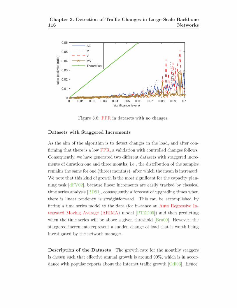
116Chapter 3. Detection of Traffic Changes in Large-Scale Backbone
Networks
0 0.01 0.02 0.03 0.04 0.05 0.06 0.07 0.08 0.09 0.10
0.01
0.02
0.03
0.04
0.05
0.06
significance level α
fals
e po
sitiv
es (r
atio
)
AEMVMVTheoretical
Figure 3.6: FPR in datasets with no changes.
Datasets with Staggered Increments
As the aim of the algorithm is to detect changes in the load, and after con-
firming that there is a low FPR, a validation with controlled changes follows.
Consequently, we have generated two different datasets with staggered incre-
ments of duration one and three months, i.e., the distribution of the samples
remains the same for one (three) month(s), after which the mean is increased.
We note that this kind of growth is the most significant for the capacity plan-
ning task [dFV02], because linear increments are easily tracked by classical
time series analysis [BD91], consequently a forecast of upgrading times when
there is linear tendency is straightforward. This can be accomplished by
fitting a time series model to the data (for instance an Auto Regressive In-
tegrated Moving Average (ARIMA) model [PTZD05]) and then predicting
when the time series will be above a given threshold [Bru00]. However, the
staggered increments represent a sudden change of load that is worth being
investigated by the network manager.
Description of the Datasets The growth rate for the monthly staggers
is chosen such that effective annual growth is around 90%, which is in accor-
dance with popular reports about the Internet traffic growth [Odl03]. Hence,

3.4. On-line Load Change Detection Algorithm 117
the monthly growth is approximately 6%. The quarterly growth has also been
set to approximately 6%, on attempts to make the obtained results compa-
rable, i.e., we have longer periods without changes in the quarterly growth
dataset, but the size of the staggers (which is relevant for our algorithm) are
the same in both time series. Accordingly, the theoretical number of changes
that should be detected with the algorithm in the Monthly Increments (MI)
dataset is 300 and in the Quarterly Increments (QI) dataset is 100.
Results In Figure 3.7(a), we show the number of detected changes on the
MI data as a function of the significance level of the performed tests. Note
that an increase in the significance level implies that the test is comparatively
less restrictive and the critical region is larger, resulting in more detected
changes. This figure shows very promising results, because the number of
detected changes is in the range 295-310, while the correct value is 300. In
addition, the number of false negatives is small for all the significances tested.
0 0.02 0.04 0.06 0.08 0.10
50
100
150
200
250
300
350
Significance level α
No.
of D
etec
ted
Cha
nges
Monthly increments
Detected
Theoretical
(a)
0 0.02 0.04 0.06 0.08 0.10
50
100
150
200
250
300
350
Significance level α
No.
of D
etec
ted
Cha
nges
Quarterly increments
DetectedTheoretical
(b)
Figure 3.7: Detected changes in the staggered increments dataset: (a)Monthly Increments dataset; (b) Quarterly Increments dataset.
Figure 3.7(b) presents the same information but for the QI data. We note
that the algorithm performance decreases. There is no significance level at
which we detect exactly the same number of changes that are theoretically in
the dataset. In addition, the false positives have enlarged, being now greater
than 50. With significance values larger than 0.06 we detect more than 300
changes, meaning that for every theoretical change, we alert for 3 detected

118Chapter 3. Detection of Traffic Changes in Large-Scale Backbone
Networks
changes. We will shed light on the causes of this misidentification in the
following paragraph by inspecting the results at a fixed significance level.
Analysis at Fixed Significance Level
We now further inspect the results of the validation, but with a fixed value
for the significance level. The value selected for the significance level is
α = 0.05, as it is the most commonly used value. By making the significance
level fixed, we can apply the analysis of the Hotelling’s T 2 statistic presented
in Appendix C. In addition, we can present graph plots of the clusters found
and inspect the reported change points. On those graphs, we plot the values
of the projection in one vector component, using different color and marker
combinations to differentiate the change-free regions according to the results
of the algorithm. Furthermore, we mark with a straight horizontal line the
mean of all the values within a change-free region, which makes it for judging
the validity of the reported change points. As the amount of points generated
for each vector component is huge, we will focus on certain regions of the
plots that we have found to be relevant for the validation.
Datasets with no Changes To analyze the reported changes when the
input dataset has no changes in theory, we focus on the AE dataset.
In Figure 3.8(a), we show the change-free regions found by the algo-
rithm using different color-marker schemes in the first 300 samples of the
AE dataset. Although the samples are concentrated around the true mean
(100), the algorithm detected some change points. This happens because we
are applying a statistical test, whose confidence level can be interpreted as
the FPR in the limit.
The change points reported by the algorithm in this dataset can be due to
the following reasons: (i) The algorithm found one cluster with mean above
the theoretical value followed by a cluster with mean under the theoretical
value (or vice versa). This can be easily seen between the first two change-
free regions in Figure 3.8(a); (ii) the weighted sum of the differences in all
the vector components is above F 1−α0p,N−p (Appendix C). To illustrate this fact,
we present in Figure 3.8(b) the same zoom area for vector component 2. The

3.4. On-line Load Change Detection Algorithm 119
0 50 100 150 200 250 30092
94
96
98
100
102
104
106
108Time Series of AE vector component 1
Samples
Val
ue
(a)
0 50 100 150 200 250 30090
95
100
105
110
115Time Series of AE vector component 2
Samples
Val
ue
(b)
Figure 3.8: Time Series representation of the change-free regions for the first300 samples: (a) 1st vector component of the AE dataset; (b) 2nd vectorcomponent of the AE dataset.
differences between the last two change-free regions on Figure 3.8(a)–(b) (the
dots (·) around sample 200 and the circles (◦) on its right) are very small, but
the addition of these differences through all the variables produces a change
point—this is in fact an advantage of the statistical procedure used in our
algorithm: MBFP tests for differences in the mean taking into account the
variations in all the vector components at the same time.
Datasets with Staggered Increments These datasets are designed to
be invariant both in mean and variance for a fixed period of time, after which
the value of the mean is increased. Consequently, in these regions without
changes we are in the same case as in the AE dataset. We therefore inspect
each stair of the dataset from the point of view used for the dataset with no
changes.
The clusters in the final samples of the MI and QI datasets (sample
8000 and above) are easily identified by the algorithm, as the differences
between those clusters are large enough due to the increment by percentage
in each theoretical change point. Therefore, we will zoom in the beginning
of the datasets and focus on the first samples—the four first change-free
regions. Such regions are depicted in Figure 3.9(a) for the MI dataset and
Figure 3.9(b) for the QI dataset, where we have placed vertical lines in the
time instants where the theoretical change points are located.

120Chapter 3. Detection of Traffic Changes in Large-Scale Backbone
Networks
0 30 60 90 12040
50
60
70
80Time Series of MI variable 1
Samples
Val
ue
(a)
0 90 180 270 36040
45
50
55
60
65
70Time Series of QI variable 1
Samples
Val
ue
(b)
Figure 3.9: Zoom to the first four change-free regions of the 1st vector compo-nent with delimitation lines for the theoretical change points: (a) MI dataset;(b) QI dataset.
As can be seen in the figures, the variance of the samples is large enough
(compared to the mean value) to make samples in different theoretical change-
free regions (therefore with different means) to be indistinguishable in some
cases. For instance, consider the first change-free region (under sample 30)
of Figure 3.9(a). The circle (◦) samples in this region are generated with the
same mean as the dot (·) ones. However, these circle samples resemble more
to those circle samples in the second change free region (between samples
30 and 60) than to the dot ones with the same theoretical mean. This is
detected by the algorithm through the clustering technique, which divides
the first region before the theoretical change. As the difference between the
means is truly significant, the MBFP procedure detects it and a change point
is reported between these clusters. That is a visual example that shows how
the algorithm misses the true location of the change point between those
regions, which we have also observed in other instants of the dataset. This
rationale explains all the false positives detected by the algorithm, that un-
der small variance samples or with a more restrictive significance value would
have been detected in the right time instant. However, if we pay attention
to the second change-free region, we find that there are no significant differ-
ences between the two clusters found by the algorithm when inspecting them
visually. Note from C that the detected change point between these two
clusters is also due to the differences in the means of the remaining vector

3.5. Change Point Analysis with RealNetwork Measurements 121
components, although apparently in this component there is no change.
In the QI dataset (Figure 3.9(b)), in each theoretical change-free region
our algorithm reported several change points. The reason for the detection
of these extra change points is the same pointed out for the AE dataset, as
the extra change points are detected within a theoretical change-free region,
where the mean and the variance remain constant. On the other hand,
there are some theoretical change points not reported by the algorithm—for
instance the one in sample 270. The explanation for this misidentification
is the same as in the MI dataset—i.e., the variance of the samples is high
compared to their mean.
Consequently, if we focus on the detected change points that cannot be
attributed to the inherent FPR of the statistical test given by its signifi-
cance, the performance of our algorithm with different kinds of datasets is
satisfactory because the number of change points detected is approximately
the same than in our ground truth datasets. There is still a little devia-
tion in the location of the change points, but such deviation is small enough
compared to the length of the change-free regions (we have location errors
smaller than 5 days, whereas the change-free regions are larger than 25 days
in average), and therefore its effect is not truly relevant for traffic engineer-
ing tasks performed by network managers. Actually, the aim of our change
point detection technique is to identify links with a changing stationary traf-
fic behavior and not sudden load increases, which are usually detected with
threshold-based management systems.
3.5 Change Point Analysis with Real
Network Measurements
In this section, we present the results of applying our change point detection
methodology (Section 3.4) to the real network measurements of Section 3.2.1.
Table 3.5 summarizes the number of tests performed and alerts generated by
our algorithm when applied to such dataset, which is three-year long. The
second column shows the number of times the MBFP testing methodology

122Chapter 3. Detection of Traffic Changes in Large-Scale Backbone
Networks
was applied. This is the number of times that the clustering algorithm found
potential change points. The third column shows the number of times an
alert was generated—i.e., the number of times the null hypothesis of equality
of means was not satisfied. The values on the left of the slash refer to the
incoming direction, and the ones on the right to the outgoing direction.
Table 3.5: Results of the on-line algorithm (Incoming/Outgoing).
LinkNumber Number
LinkNumber Number
of tests of alerts of tests of alerts
U1 68/130 12/9 U2 112/75 10/12U3 64/84 11/11 U4 79/59 10/12U5 62/75 13/11 U6 108/61 10/11U7 86/57 10/11 U8 73/84 10/10U9 68/76 13/11 U10 82/94 11/13B1 85/89 11/10 B2 98/85 8/9B3 56/76 11/12 B4 59/57 12/11B5 123/88 10/11 X1 65/102 11/12X2 67/67 11/12 X3 103/75 9/11
The advantage of our on-line algorithm to network load detection is that
it decreases the OPEX by reducing the human supervision. We remark
that our algorithm produces an alert only in case a stationary change in
the load happens. The rest of the time the link is considered normal and no
intervention from the network manager is required. Taking into account the
duration of the measurement campaign, our algorithm placed less than 13
network load change alerts requiring human supervision in a period of more
than 750 days (including holidays), which means a load change nearly every
two months in average. We also show in Table 3.6 the average values for
both the number of tests and the number of alerts in both directions, when
grouped by link type, and the total average of such quantities.
To illustrate these results, we present in Figure 3.10 the obtained clusters
using the color-markers scheme of Section 3.4.3 for different links. More
specifically, we show the results for the time interval 10:30-12:00 (variable
8), because it is the busiest interval. Figure 3.10(a)-(b) show the results for
U1 for the incoming-outgoing direction, respectively. Figure 3.10(c)-(d) show

3.5. Change Point Analysis with RealNetwork Measurements 123
Table 3.6: Average of the on-line algorithm results (Incoming/Outgoing).
Link type Number of tests Number of alerts
University 80.20/79.50 11.00/11.09Backbone 84.20/79.00 10.40/10.60eXchange 78.33/81.33 10.33/11.66
Total 80.94/79.67 10.72/11.06
the results for B1 and finally Figure 3.10(e)-(f) show the obtained clusters
for the X1. We have selected these links because we have found them to be
representative.
As it turns out, nearly all the clusters obtained by the algorithm and
shown in the figures are reasonable. However, there are some reported clus-
ters that do not seem to have been properly detected. It is worth recalling
the rationale followed in the validation of the algorithm, i.e., that a reported
change point can be due to differences in different variables than the one
shown.
To further analyze the results of the change detection algorithm, we cre-
ated a binary time series with the change points reported by the algorithm
for each direction of each university link. Such time series has a 0 value
during a change-free region (where we have also included holidays), whereas
the change point instant is marked with a 1. For each of these time series, we
have computed the Sample Autocorrelation Function (SACF) to find possi-
ble periodicities. Furthermore, in order to assess whether an autocorrelation
coefficient ac at a given lag l0 is significant, we have also delimited the 99%
confidence interval for the null hypothesis H0 : ac(l0) = 0 with horizontal
straight lines. Therefore, those lags l with ac(l) outside this region signifi-
cantly differ from 0. We show in Figure 3.11(a) an example of the results
from link U1, as we have found it to be representative of the set of SACF.
In that figure, we see that there is some periodicity in the binary change
point time series, because there are significant autocorrelation coefficients at
lags approximately multiple of 50. However, such periodicity does not mean
that the changes in the load are periodic, but that the restrictions of the

124Chapter 3. Detection of Traffic Changes in Large-Scale Backbone
Networks
0 50 100 150 200 250 3000
50
100
150
Days
Load
(Mbp
s)
(a)
0 50 100 150 200 250 300
20
40
60
80
100
Days
Load
(Mbp
s)
(b)
0 50 100 150 200 250 3000
500
1000
1500
Days
Load
(Mbp
s)
(c)
0 50 100 150 200 250 300
200
400
600
800
Days
Load
(Mbp
s)
(d)
0 50 100 150 200 250 3001000
1500
2000
2500
3000
3500
4000
Days
Load
(Mbp
s)
(e)
0 50 100 150 200 250 300
1000
1500
2000
Days
Load
(Mbp
s)
(f)
Figure 3.10: Change points found by the on-line algorithm on the time in-terval 10:30-12:00: (a) Incoming direction of link U1. (b) Outgoing directionof link U1. (c) Incoming direction of link B1. (d) Outgoing direction of linkB1. (e) Incoming direction of link X1. (f) Outgoing direction of link X1.

3.5. Change Point Analysis with RealNetwork Measurements 125
algorithm (i.e., that the changes must be sustained for more than two weeks)
affect the randomness of the time between change points. Therefore, we can
conclude that the changes in the load are not subjected to certain relevant
events, like the change between months or academic seasons.
0 100 200 300 400 500 600 700−0.2
0
0.2
0.4
0.6
0.8
Lag (days)
Sam
ple
Aut
ocor
rela
tion
(a)
−20 −10 0 10 20−0.2
0
0.2
0.4
0.6
0.8
Lag (days)S
ampl
e C
ross
Cor
rela
tion
(b)
Figure 3.11: Correlations functions of the binary time series (including hol-idays): (a) Sample Autocorrelation Function (SACF) of the outgoing di-rection of U1. (b) Sample Cross-correlation Function (SXCF) between theincoming and outgoing direction of U1.
In addition, we also computed the Sample Cross-correlation Function
(SXCF) between the incoming and outgoing directions of each university
link. The results show that only 3 out of the 18 total links have no signif-
icant cross-correlation coefficient xc within 5 lags, determined by the same
criteria used with the SACF. This means that the changes in the loads of
the incoming and outgoing directions of the same link are usually correlated,
and are detected by the algorithm within a small difference of days. Such
result is expected, as the main important facts impacting the load of a link
are traffic engineering tasks, such establishing/changing routes or upgrading
link capacities, and variations in the number of users accessing the network
or in the intensity of usage. On the other hand, we envisage that when the
changes are asymmetric (i.e., there appears a change in one direction but not
in the other one), such changes are mainly due to shifts in the way the users
access the network or their preferred applications—behavioral changes. For
instance, some Internet users are gradually moving from Peer-to-Peer (P2P)
applications, where received and sent traffic are approximately in the same

126Chapter 3. Detection of Traffic Changes in Large-Scale Backbone
Networks
order of magnitude, to one-click hosting services, where large amounts of
traffic are downloaded whereas the uploaded traffic is negligible for the most
of the users [AMD09]. An example of the SXCF is shown in Figure 3.11(b)
again for university U1. We show in that figure only the range of ±20 lags
from the origin, which is enough given the periodicity exhibited by the SACF
shown in Figure 3.11(a).
3.6 Network Management Based on Relevant
Events
In this section we present a network management system that uses the change
point detection algorithm—i.e., it shows the relevant events that potentially
need action by the network manager. We develop an alert color code to
differentiate the importance of the detected changes, which allows us to create
weather maps of the operator’s network showing the most conflictive links
that may be eligible for capacity planning and traffic engineering tasks. As
it turns out, when the algorithm detects a change point, it only reports its
location, but not any measure of its relevance. Obviously, the impact of
a change in the load in the busy hour is not the same as if the change is
produced in the midnight. To differentiate such changes, once our algorithm
has detected a change point, we apply a univariate normality test for the
differences in the means of each variable of the reported clusters. We do
so because the MBFP methodology does not distinguish between variables,
but takes the overall effect into account. As a consequence of the multiple
testing, we apply the Bonferroni correction [Hay05, page 386] to maintain the
familywise error rate, thus setting the corrected significance level to αc = α/p,
where α is the desired probability of Type I Error and p is the number
of tests, which in our case equals the dimension of the distribution. For
those univariate tests, we use the Welch’s t test [Wel38], which is the most
widely used approximation to the Behrens-Fisher problem in the univariate
case. These multiple tests determine which of the variables has experienced
a change. Consequently, we can establish an alert color code, depending on

3.6. Network Management Based on Relevant Events 127
which variables are known to have a change in their means and taking into
account the daily pattern of the link (Figure 3.2).
The alert color code contains five different colors. The variables and time
intervals such colors are related to are presented in Table 3.7. Consequently,
when we detect a change point, and this is motivated by a change in the
variables where the load is higher, we mark such link with red color, we do the
same using orange when the change is in a medium load variable, and using
yellow when the load is low—during nighttime. Finally, if there is no change
point, we mark the link as green, meaning that it remains stable. When we
encounter a conflict, i.e., changes happening in two or more variables with
different color codes, we mark the link with the most restricting color—i.e.,
we use the color assigned to the change in the variable with higher load. In
addition, chances are that no significant change is detected by the Welch’s t
test with the Bonferroni correction—for instance, if the change where due to
small differences in all the vector components. If this happens, we mark the
link using a blue color.
Table 3.7: Alert color code for network surveillance.
Color Meaning Variables Time period
Red Change in a high load variable 7-9 09:00-13:30Orange Change in a medium load variable 10-13 13:30-19:30Yellow Change in a low load variable 1-6, 14-16 19:30-09:00
BlueChange detected by the MBFP not
- -found by the multiple comparisons
Green No change detected by the MBFP - -
Note that the links marked with a color different than green would require
human supervision. Once the network manager becomes aware of the alert, it
can be disabled because either the change is not considered relevant enough
to take any action or the actions have already been carried out. To illustrate
the alert based system, an example of such map is presented in Figure 3.12
using the RedIRIS network architecture showed in Figure 3.1. In this exam-
ple, one link is marked with red color, meaning that in the corresponding
link, a change in a variable with high load was detected. We also have two

128Chapter 3. Detection of Traffic Changes in Large-Scale Backbone
Networks
links marked with orange color, corresponding to changes in medium load
variables, and two other links marked with yellow color corresponding to
changes in low load variables. Remember that in the link marked with red
color, chances are that there were changes also in other variables, but the
red alert prevails because it is the most important. In addition, there are
two links marked with blue color. In such links, a change in the load was
detected by the MBFP procedure. However, such change was due to small
contributions of the differences in all the vector components, and no change
was found by the Welch’s t test. Finally, the remaining links are marked with
green color, meaning that there is no change detected in those links, which
are then considered to remain stable.
��������
�������������
����������
������
��������������
����������
��������������
�����
Figure 3.12: Sample weather map of the RedIRIS network, with some linksneeding the network manager attention.
This way of visualizing the relevant events in the whole network facili-
tates large-scale network operators the surveillance of the network, allowing
them to reduce the OPEX expenditures or to move staff from the network
supervision center to link locations, in order to take action to respond to the
relevant events in a faster way.

3.7. Summary and Conclusions 129
3.7 Summary and Conclusions
In this chapter, we have presented an on-line load change detection algorithm,
which uses clustering and statistical techniques to identify statistically sig-
nificant load changes. The algorithm is based on a multivariate fairly normal
model, which keeps track of the well-known daily pattern of the network, in
order to make the statistical inference. We have validated the suitability of
that distribution to model the daily pattern and make inferences about the
means of the distribution.
The application of our methodology to real network measurements avail-
able from the Spanish academic network shows promising results, allowing
the network operator saving OPEX expenditures by reducing the visual in-
spection of the traffic time series. Finally, we have presented an alert color
code scheme that allows to manage the network focusing only on the relevant
events detected by the algorithm. To facilitate this task, visual maps of the
network are used as visualization tool of the algorithm’s output. This efficient
way of network-wide monitoring permit the service providers to guarantee
the required levels of QoS, as established in the corresponding Service-level
Agreement (SLA).


Chapter 4
Weekly Pattern Timeseries
Detrending: The Case of VoIP
Quality of service and of experience are very important and have consequently
attracted a lot of attention from the research community, specially for Voice
over IP (VoIP) services. The most impacting performance degradation for
VoIP comes from packet losses, which are mainly due to overload periods.
Consequently, timely detection of overload periods is crucial for management
of VoIP services and allows a reduction of expenses. The monitoring of actual
measurements for detecting overload periods lacks the existence of detrend-
ing models that remove the non-stationarity from the data. In this chapter,
we propose a detrending methodology tailored for VoIP services that removes
the trend from actual measurements and permits the application of the broad
family of statistical techniques that assume stationary data. To show the per-
formance of the methodology, we have designed an outlier-friendly anomaly
detection algorithm that signals anomalies after outlier removal. Further-
more, as the residuals of the detrending methodology exhibit large correla-
tions, we have proposed an alternative measurement methodology to monitor
Poisson-nature arrival processes, such as the process of call arrivals in a
VoIP system. The proposed technique outperforms the traditional one for
heavy-tailed service times, which we have demonstrated to be the case of the
actual measurements analyzed in this chapter.
131

132Chapter 4. Weekly Pattern Timeseries Detrending: The Case of
VoIP
4.1 Introduction
Quality of Service (QoS) and Quality of Experience (QoE) are very important
for Network Operators and Service Providers (NOSP), and have consequently
attracted a lot of attention from the research community [SJ11, MA06]. This
is specially the case of VoIP services, for which low values of QoS related
metrics (latency, packet loss and jitter) are crucial in order to enable its
deployment [KP09]. Furthermore, the users perception of these network
characteristics may foster the usage of the service, thus increasing service
providers revenue. With regards to the VoIP service, which we take as lead-
ing example in this chapter, the most impacting performance degradation
comes from packet losses [BMPR10]. Packet losses are mainly due to over-
load periods—i.e., time periods where the network devices are not able to
cope with the amount of load injected into the system. Furthermore, over-
load periods also have an impact on the latency and jitter, increasing the
values that may be observed during low occupancy periods. Consequently,
timely detection of overload periods is crucial for the management of VoIP
services [MZ11]. Timely detection of overload periods allows anticipation of
quality degradations and enables proactive network management [CCM+11].
To this end, NOSP are investing large amounts of money in capital and
operational expenditures. Capital Expenditures (CAPEX) are in the form
of new network devices capable of coping with the ever increasing speed in
network links, mainly in the form of active and passive probes that gather
network traffic measurements at different points in the network [CCM+11],
and high performance servers able to analyze the gathered measurements in a
centralized way [CMGD+11]. On the other hand, Operational Expenditures
(OPEX) are devoted to maintain such network devices and to hire network
managers capable of detecting and troubleshooting network problems. Given
this large investment, we have proposed an automated technique to reduce
OPEX by supporting the network monitoring tasks in Chapter 3. In order to
provide this support, the automated technique relies on the statistical analy-
sis of network traffic measurements. However, network traffic measurements
are not stationary. Instead, there is typically a day-night pattern, at which

4.1. Introduction 133
traffic loads are large during daytime and decrease at nighttime. This traffic
patterns are a consequence of users’ behavior, whose activity is reflected in
the amount of traffic observed in the network.
The lack of stationarity in network measurements, which is a common as-
sumption in the main statistical techniques, is a serious disadvantage when
analyzing network traffic measurements. As a consequence, direct appli-
cation of such statistical techniques to network traffic measurements may
lead to erroneous conclusions [DG06], such as large amounts of false posi-
tives/negatives. Therefore, we propose an unsophisticated methodology for
removing the inherent daily pattern in network traffic measurements, tailored
for VoIP call counts data. The methodology is based on some properties of
the call arrival process, which we prove to be time-varying Poisson in our
case study. The idea behind the proposed technique is simple. We com-
pute an estimate of the average daily pattern by means of a moving average
procedure. Such procedure has been proved to be fairly accurate for pre-
diction purposes [Tay08]. After the average daily pattern is computed, it is
subtracted from the actual measurements. In the end, we standardize the
result dividing the difference by the square root average pattern—which is
the standard deviation of the measurements given the Poisson nature of the
process. The output of the methodology are standardized samples (i.e., zero
mean and unit variance) that follow a normal distribution in the case the
amount of load in the network is considerable. Accordingly, we have ob-
served that the performance of the methodology improves when the night
periods are removed from the original sample. The night period removal
has no unfavorable consequences for our goals because the chances that an
overload period happens during night are negligible. However, we observed
that there are large correlations between the output samples, which evidences
lack of independence. As independence is typically an assumption for many
statistical techniques as well, such large correlation may spoil the results of
the statistical analysis applied. We investigated further such correlations,
and designed an alternative measurement methodology that yields smaller
correlations in some cases, which depend on the nature of the call holding
time distribution, than the traditional measurement methodology for Poisson

134Chapter 4. Weekly Pattern Timeseries Detrending: The Case of
VoIP
processes. Specifically, we show that when the call holding time distribution
follows a Pareto or log-normal distribution, there is a high probability that
our proposal outperforms the traditional one, which eventually depends on
the actual parameters of such distributions. Furthermore, we show that the
best fitting model for the call holding times is a mixture of two log-normals
and a Pareto distribution in our dataset. In addition, we present a numerical
evaluation which shows that the proposed alternative outperforms the tradi-
tional measurement methodology in terms of correlations if the call holding
time is distributed accordingly to the best fitting model.
On attempts to show the performance of the proposed trend removal tech-
nique, we propose an on-line oulier-friendly anomaly detection algorithm.
The algorithm removes outliers before signaling anomalies taking into ac-
count the likeliness of each model’s residual. The algorithm is able to detect
both shortages and overload periods, as well as shifts in users’ behavior.
The structure of the rest of the chapter is as follows: Section 4.2 presents
the related work. Mainly, we surveyed the forecasting techniques that have
been proposed for predicting call count measurements, and summarize the
models suggested in the literature to fit the arrival process and holding time
distribution of VoIP calls. Afterwards, a description of the dataset and its
daily pattern is presented in Section 4.3, along with the results of model-
ing the call arrival process and its duration distribution. After describing in
detail the proposed methodology to remove the trend from VoIP call count
measurements and assessing the validity of its theoretic assumptions in Sec-
tion 4.4, we propose the alternative measurement technique and present its
evaluation in Section 4.5. Next, we provide in Section 4.6 a description of
the anomaly detection methodology and the results of its application to the
measurement dataset after the seasonality is removed. Finally, Section 4.7
concludes the chapter.
4.2 Related Work
The traffic patterns in telecommunication systems have been analyzed for
more than a decade [TMW97], and even its evolution throughout time has

4.2. Related Work 135
been studied [Hee07]. Such patterns appear as a response to users’ behavior,
and are commonly referred in the literature with the term daily pattern. The
daily pattern varies depending of the kind of users that access the network,
although it can be deemed as invariant (i.e., having a similar shape from day
to day) when the kind of users is fixed. These users can be divided into two
main groups. On one hand, we have enterprise users—users that access the
network in their workplaces. The daily pattern that they produce is directly
related to the office working hours, i.e., the load is larger during working
hours, and usually there appear two clearly distinguishable peaks—before
and after lunchtime. A study of this kind of daily pattern can be found
in [MGDA10] for the Spanish Academic Network RedIRIS1 and was briefly
presented in Section 3.2.2. On the other hand, we have domestic users—users
that access the network from their residence. This pattern is also influenced
by the working hours, but in an opposite way: the load is larger after usual
working hours, when users come back from their workplaces. Such usage
pattern has been studied within the TRAMMS European project [ALK+09,
ALS+10].
This shape invariance of the network traffic measurements is also ob-
served at different timescales. For instance, if we compare measurements
in a weekly basis, we can observe that the shape of the pattern is approxi-
mately the same from Monday to Thursday. On Fridays, we observe a scaled
version of the other working days pattern—i.e., the shape is the same, but
the load is usually smaller. Finally, on weekends and holidays, we found
almost flat patterns when dealing with enterprise measurements. The main
reason for this flat pattern is that the traffic during weekends is principally
due to applications that are left running and generate traffic without user
interaction.
A similar traffic pattern can be observed when taking into account only
VoIP traffic [BMPR10, Hee07]. However, the studies of VoIP traffic have put
more effort on analyzing the call characteristics, namely the call arrival pro-
cess and the call holding time distribution, rather than focusing on the daily
or weekly patterns. Regarding the call arrival process, it is widely accepted
1http://www.rediris.es/index.php.en

136Chapter 4. Weekly Pattern Timeseries Detrending: The Case of
VoIP
that it is fairly well modeled by a time-inhomogeneous Poisson process, which
can be considered stationary at short timescales, ranging from scores of min-
utes to hours [Hee07, BMS+04, BGM+05]. In this line, there have been
studies in the literature proposing methods for estimating the parameters of
such processes [MPW96], assessing the validity of such assumption by means
of statistical tests [BGM+05, BMS+04, BZ02], and even adapting traditional
queuing-theoretic models to this arrival process [Mas02]. In our study, we use
the test presented in [BGM+05] to validate the time-inhomogeneous Poisson
arrival process assumption in our dataset. The details of the test are de-
scribed in Section 4.3.2. Conversely, there is no consensus in which model
provides the best fit to the call holding time distribution. However, the fact
that the holding times are no longer appropriately modeled by means of expo-
nential distributions has been widely proved. The distributions proposed in
the literature are manifold. Examples of this are the hyper-exponential dis-
tribution [Hee07], the inverse Gaussian distribution [BMPR10], the Weibull
distribution [CK02], the Pareto distribution [DSM04], and the log-normal
distribution [CHL07]. In our case study presented in Section 4.3.3 we show
that the best modeling distribution is the log-normal distribution, although
higher goodness-of-fit is achieved by a mixture model composed of two log-
normal and one Pareto components.
On the context of call centers, the main research efforts have focused
on providing an accurate forecast of the time series of call arrivals [ADL04,
SH05, SH08a, SH08b, Tay08]. Avramidis et al. [ADL04] propose three dif-
ferent models for this task. The proposed models are parsimonious, in the
sense that the number of parameters is small, which make them useful for
on-line methodologies. However, the timescale of prediction is larger than
two weeks which is useful for staffing of call centers, because the agents must
know their assignment two weeks or more ahead, but not for our purposes—
we work with complete weeks, or the weekly pattern, and require one-week
lead time forecasts. Shen and Huang [SH08b, SH05, SH08a] apply Singular
Value Decomposition (SVD) to reduce dimensionality and denoise the time
series before forecasting, by leveraging on the significant singular values. The
SVD is also useful for anomaly detection as showed in Section 2.2. However,

4.3. Measurement Dataset 137
such anomaly detection is achieved through visual inspection of the singu-
lar values, which makes it useless for application in automated detection
methodologies, and the timescale of detection is in the range of days, which
is useful for forensic network analysis, but not for on-line and timely reac-
tion. In [SH08b], Shen and Huang improve the forecasting methodology by
dynamically updating the forecast with intraday information. Such updates
reduce the prediction error, but at the expense of larger model complexity.
A comparison of univariate time series methods is presented in [Tay08]. This
comparison includes naive methods such as moving average—which is the
approach we follow in our methodology.
All in all, the more complex methods achieve the smaller prediction error
in few-days ahead forecasting, but simpler methods such as moving average
achieve similar prediction errors for one week lead times and are computa-
tionally more tractable.
4.3 Measurement Dataset
Experiments in this chapter are using actual traffic traces collected from an
operational network. Using Tstat [FMM+11], Internet Protocol (IP) traffic
exchanged by customers was measured in a large Point of Presence (PoP) of
an NOSP in Italy where VoIP is deployed. A total of 22,000 customers were
continuously monitored for more than 4 months, starting from November
2010. Tstat is used to identify VoIP flows, i.e., voice calls, and to extract
several performance indexes for each call [BMPR10]. The measurements were
kindly donated by the Telecommunication Network Group of Politecnico di
Torino, in compliance with data privacy preserving regulations.
In particular, in the context of the present chapter we are interested in
the call arrival process and call holding time distribution. The resulting
dataset contains the log of the call arrival epochs and the corresponding du-
rations. Later in this chapter, we statistically analyze these, and use the
resulting processes/distributions to assess the performance of our methodol-
ogy. This dataset containing start and end times of the calls will be referred
to as detailed below. On the other hand, the dataset containing the count

138Chapter 4. Weekly Pattern Timeseries Detrending: The Case of
VoIP
process of the number of calls being active is referred to as summarized in
what follows. It is used to estimate the average pattern, apply our proposed
detrending model and analyze the residuals for deviations of normality that
may signal anomalies in the network.
4.3.1 Daily and Weekly Patterns
In this section we present the average daily and weekly patterns of the VoIP
measurements we use in the following sections. As can be seen in Figure 4.1,
the daily and weekly patterns are very much alike to those of the RedIRIS
network presented in Section 3.2.2. The daily pattern exhibits two peaks,
before and after lunchtime, typical of enterprise networks. Although the
measurements come from residential networks, such behavior is expected
in VoIP data. Regarding the weekly patter, we again observe the typical
pattern of enterprise networks, having working days similar shape among
them. However, the weekends have an scaled version of the weekday pattern
instead of having a flat pattern such as the observed in enterprise networks.
Number
ofcalls
Monday Tuesday Wednesday Thursday Friday Saturday Sunday
50100150200250300350400450500
Figure 4.1: Average weekly pattern of the analyzed dataset.
4.3.2 Call Arrival Process
Classical theoretical models for voice traffic posit that the call arrival process
is Poisson distributed. Such process results when there is a large number of
users generating calls independently of each other. However, this simple

4.3. Measurement Dataset 139
model does not usually apply to actual measurements, commonly explained
because the users’ behavior varies during the day. To cope with such users’
behavior variation, non-homogeneous Poisson processes are used instead—
in which the intensity of call arrivals is time dependent. In practice, this
time-varying condition is relaxed, and the process rate is assumed to remain
constant for blocks of time—i.e., the process is considered to be short-term
stationary. We conjecture that the arrival process in our dataset is time-
varying Poisson in this sense, and thus the intensity remains constant for
time-blocks of length L. In our particular case, we need L ≥ 300 seconds to
prove the validity of equation (4.4).
To assess the correctness of our model, we apply to our detailed dataset
a test presented by Brown et al. in [BGM+05] specifically designed to sta-
tistically prove whether the arrival rate is constant within each given time
block. To construct the test, the interval of a day is split into disjoint blocks
of length L, resulting in a total of I blocks. With this setup, let Tij be the jth
ordered arrival time in the ith block. Denoting with J(i) the total number of
arrivals within the ith block, we then define Ti0 = 0 and
Rij = (J(i)+1−j)(−log
( L− Tij
L− Ti,j−1
)), j = 1, . . . , J(i); i = 1, . . . , I. (4.1)
The {Rij} will be independent standard exponential variables under the
null hypothesis that the arrival rate is constant within each block. We note
that the null hypothesis does not assume that the arrival rates of different
blocks have any pre-specified relationship, and refer the interested reader to
the original publication [BGM+05] for a proof of the test.
In Table 4.1 we present the results of applying the test to different block
sizes L. We use the Kolmogorov-Smirnov (KS) test to verify the null hypoth-
esis at 5% significance level—see Appendix A for a brief description of the KS
test. The results presented in the table show that the arrival process can be
regarded as fairly time inhomogeneous Poisson only at very short timescales,
say less than 10 minutes, which is enough to justify such an assumption in
our methodology.

140Chapter 4. Weekly Pattern Timeseries Detrending: The Case of
VoIP
Table 4.1: Results of the inhomogeneous Poisson arrival process assessment.
Block lengthRejection %
Block lengthRejection %
L (min) L (min)
90 73.93 30 35.3275 69.24 25 27.0460 61.34 20 19.0945 49.55 15 14.0840 43.88 10 9.3935 38.94 5 6.90
4.3.3 Call Holding Time Distribution
In this section we study the Call Holding Times (CHT) in our sample, aiming
at finding the model which best fits the service-time duration distribution.
The literature posits that the CHT distribution is no longer appropriately
modeled by an exponential distribution, and several alternatives have been
proposed. The majority of them are heavy-tailed distributions for the VoIP
service, which may be explained given the low (usually flat) rates at which the
service is commercialized. After a visual inspection, it turns out that a heavy-
tailed distribution is the more likely distribution to fit our detailed dataset
as well. In this visual inspection, we have used log-log plots of the empirical
Complementary Cumulative Distribution Function (CCDF) of the sample,
which allow us to gain insight in the tail of the distribution. Consequently,
we particularly restrict in our Goodness of Fit (GoF) assessment to heavy-
tailed distributions, in the sense that the distribution has heavier tails than
the normal distribution. To measure the GoF we use again the KS statistic,
although in this case testing for the null hypothesis that the sample comes
from the hypothesized distribution is not possible. As we are estimating the
parameters of the hypothesized models from the sample, the critical values
determined in this way are invalid [Dur73]. However, we still can use the KS
statistic as a measure of model discrepancy, which will allow us to select the
best fitting model.
Table 4.2 summarizes the results of the GoF study. In that table, we
present the models which evidenced better fit to the data sorted by the value

4.3. Measurement Dataset 141
of the KS statistic (the shorter the better), along with the MLEs of the
corresponding parameters.
Table 4.2: GoF results for different fitting models.
Distribution Parameters KS statistic
Pareto Log-normal1 Log-normal2
0.0046Pareto p = 0.6793 p = 0.2023 p = 0.1184
+ k = 0.2749 μ = 6.0857 μ = 3.54102 log-normal σ = 63.1607 σ = 0.9523 σ3 = 0.5201
Log-normal1 Log-normal2 –
0.00742 log-normal
p = 0.1089 p = 0.8911μ = 3.6421 μ = 4.2926σ = 0.4810 σ = 1.5528
Weibull Log-normal –
0.0075Weibull p = 0.0968 p = 0.9032
+ λ = 42.7199 μ = 4.2964log-normal k = 2.4978 σ = 1.5385
Log-normal – –
0.0246p = 1
Log-normal μ = 4.2218σ = 1.4882
Figure 4.2(a) shows the log-log plot of the empirical CCDF of the data
along with the models presented in Table 4.2. Accordingly with the quanti-
tative results, we can observe in the figure that the best fit is provided by the
mixture of two log-normal and one Pareto distributions. This mixture model
is capable of fitting the whole body of the data, but there is a lack of fit in the
very end of the tail. Furthermore, we can observe a small oscillation in the
data tail, which is not captured by any of the fitting models. However, this
can be just an artifact provoked by the sample size. Although the number
of samples is large (>1 million of samples) for usual purposes, it may not be
enough to accurately estimate the probabilities in the tail, since those events
are rather unlikely. To shed light to this fact, we computed a distributional
envelope for the log-normal fitting model, which shows the high variability
that the log-normal distribution can have in the tail. Concretely, we gen-

142Chapter 4. Weekly Pattern Timeseries Detrending: The Case of
VoIP
erated N = 1000 populations of size s =100K samples from a log-normal
distribution with the same parameters that provide the best fit. We com-
puted the empirical CCDFs of these populations, and plotted them jointly
with the data and the log-normal best fitting model in Figure 4.2(b). In that
figure we can observe that the actual measurements lie within the simulated
envelope. Consequently, we can conclude that the actual measurements are
a plausible realization of the best log-normal fitting. We note that in fact,
according to Table 4.2, there are models that provide even better fit to the
actual data. This means that the situation is even better if other models are
taken into account.
Call length (s)
P(X
>x)
Data2 log-normalWeibull + log-normalPareto + 2 log-normal
100 101 102 103 104 10510−8
10−6
10−4
10−2
100
(a)
Call length (s)
P(X
>x)
Simulated envelope
Actual dataLog-normal fit
10−2 10−1 100 101 102 103 104 105 10610−8
10−6
10−4
10−2
100
(b)
Figure 4.2: Log-log plots of the data: (a) log-log plot of the data and the bestfitting models according to the KS statistic value; (b) log-log plot of the dataalong with the best log-normal fit and its simulation envelope.
4.4 Detrending Methodology
In this section, we provide a methodology to remove the inherent seasonality
that exists in network traffic measurements. After its description and justifi-
cation, we present an analysis of its performance and the achievement of the
expected results.

4.4. Detrending Methodology 143
4.4.1 Methodology Description and Expected Results
Our methodology exploits the practical invariance of the weekly pattern to
estimate and remove the seasonality from the measurements. We assume
a set-up where the measurements are time series of traffic counters (byte
counts, number of active calls, etc.) at a given time granularity. In our
analysis, we will use a five-minute time granularity, because it is the usual
timescale for many tools that output network traffic measurements—e.g.,
the Multi Router Traffic Grapher (MRTG) tool [OR98]. We denote the
network traffic measurements as xni , being i = 0, 1, 2, . . . , 2015 the number
of the 5-minute interval within the week, starting on Monday midnight, and
n denoting the week number within the dataset, out of a total of N = 12
weeks. The purpose of the methodology is to provide a good estimate yn for
the measurement vector of week n, xn, using the available information from
previous weeks, xj , j < n.
We assume that the differences from week to week in the weekly pattern
are due to random deviations from an average network usage pattern, and
therefore propose the following model for the measurements
xn = α+ εn, (4.2)
where α denotes the average fixed pattern and εn are the random deviations
from such pattern. We assume that this deviations are normally distributed
with zero mean and heteroscedastic variance σ2.
The simpler approach for estimating the average pattern is to set the
prediction vector yn to a windowed average xn(w) of the measurements in
the previous weeks, assigning different weights Wj to different week lags,
being w the length of the window in weeks:
yn = αn = xn(w) =
w∑j=1
1
Wj
xn−j . (4.3)
The proposed estimation uses the arithmetic average of the measurements
in a window of size w = 5. We use this window size because it represents a

144Chapter 4. Weekly Pattern Timeseries Detrending: The Case of
VoIP
trade-off between model accuracy and robustness to pattern shifts—meaning
that the model would be able to track variations with time on the pattern
shape. On the other hand, we use the arithmetic mean (all the weights Wj
equal to the window size w) because it minimizes the Mean Squared Error
(MSE) of the estimator. Nonetheless, we have also tested different averaging
processes (for instance exponentially decreasing or increasing weights), and
the differences in performance are negligible.
We can then remove the estimated pattern from the actual measure-
ments, obtaining theoretically zero mean residuals. However, as the errors in
the model are assumed to be heteroscedastic, so will be the residuals com-
puted after trend removal. This would suppose a drawback, because many
of the main statistical tools assume homoscedasticity besides stationarity,
and therefore calls for standardization. Such standardization implies divid-
ing each residual by its standard deviation. Consequently, we would need
to design another model for estimating the pattern standard deviation. In-
stead, we exploit the distributional properties of the measurement process
to circumvent this computation. Concretely, we showed in Section 4.3.2 that
the arrival process is time inhomogeneous Poisson. As a consequence, we can
use the property relating the mean and the variance of a Poisson process to
estimate the standard deviation—for a Poisson process, the mean equals the
variance. Hence, we obtain standardized residuals rn by removing the aver-
age pattern from the actual measurements, and then dividing by its square
root:
rn =xn − yn
√yn
. (4.4)
4.4.2 Model Performance Results
We have estimated the seasonality according to equation (4.3) in our summa-
rized dataset, and computed the corresponding residuals using equation (4.4).
For the shake of brevity, we only show the results for one week, which we have
found to be representative of the performance of the model. Figure 4.3(a)
shows the estimated pattern, computed from previous weeks samples, super-

4.4. Detrending Methodology 145
imposed on the actual samples of the week under study. It shows the GoF
of the estimated pattern to the actual measurements, mainly due to the high
stability of the weekly pattern in this kind of data. The main differences ap-
pear at the peaks of the weekly pattern, at which the samples show abrupt
variations. The corresponding residuals are shown in Figure 4.4(a). The vari-
ance of the residuals seems to be higher than expected, even appearing very
large deviations from its mean—higher than 5σ. This can be better observed
in the corresponding Gaussian Quantile-Quantile (Q-Q) plot, shown in Fig-
ure 4.5(a), at which there appears deviations in the tails from the straight
line that indicate non-normality.
#calls
Monday
Tuesday
Wednesday
Thursday
Friday
Saturday
Sunday
samplespattern
0
100
200
300
400
500
600
(a)
#calls
Monday
Tuesday
Wednesday
Thursday
Friday
Saturday
Sunday
samplespattern
0
100
200
300
400
500
600
(b)
Figure 4.3: Data samples for the week under study and estimated patternbased on previous weeks data samples: (a) nights included; (b) nights re-moved.
Standardized
Residuals
Monday
Tuesday
Wednesday
Thursday
Friday
Saturday
Sunday
-10
-5
0
5
10
15
(a)
Standardized
Residuals
Monday
Tuesday
Wednesday
Thursday
Friday
Saturday
Sunday
-8
-6
-4
-2
0
2
4
6
(b)
Figure 4.4: Residuals obtained after standardization with the estimated pat-tern: (a) nights included; (b) nights removed.
The reason behind such large deviations from the hypothesized distribu-
tion is related with the night periods. During the night, the load decreases

146Chapter 4. Weekly Pattern Timeseries Detrending: The Case of
VoIP
Standard Normal Quantiles
Quan
tilesof
InputSam
ple
-4 -3 -2 -1 0 1 2 3 4-8
-6
-4
-2
0
2
4
6
8
10
12
(a) Deviations from a straight line appear inthe tail evidencing non-normality.
Standard Normal Quantiles
Quan
tilesof
InputSam
ple
-4 -3 -2 -1 0 1 2 3 4-8
-6
-4
-2
0
2
4
6
(b) Smaller deviations appear when nights areremoved.
Figure 4.5: Gaussian Quantile-Quantile plots of the residuals: (a) nightsincluded; (b) nights removed.
drastically, being nearly zero for several hours—when the majority of the
users sleep. The estimated pattern captures this behavior and causes the
residual computation to explode in the standardization step—when dividing
by the square root of the estimated pattern. To circumvent this numerical
problem, we decided to remove the night periods from the sample. Note that
for the final purpose of our methodology (i.e., detecting overload periods that
may cause system performance degradation) nights are practically irrelevant,
given that the amount of traffic is low and therefore it is difficult that sudden
changes might have an impact on the network performance.
We define the night period from midnight to 6 a.m., and remove the
related samples from the dataset—we filter out a total of 72 samples per
day. The corresponding estimated pattern and residuals are shown in Fig-
ure 4.3(b) and Figure 4.4(b), respectively. We can observe that without
nights the variance of the residuals has been reduced. This is shown also in
Figure 4.5(b), where the Gaussian Q-Q plot of the residuals without nights
is presented. As it can be observed, now the deviations in the tails are not
so large, and consequently fairly normality cannot be rejected.
However, we have observed that there is some periodical trends in the
residuals—see Figure 4.4. This may imply that there exists correlation be-
tween the residuals, violating the assumption of independence that is used in
most of the sound statistical procedures. To gain insight into this effect, we

4.4. Detrending Methodology 147
present in Figure 4.6 the autocorrelations of the residuals for both cases: in-
cluding and without including nights in the sample. Such figures confirm that
there is some periodic component in the residuals, because the autocorrela-
tion plots show some kind of oscillation. This turns out in a non-negligible
correlation, having more than 9% of the samples outside the 5% confidence
interval when nights are included and more than 7.5% when night periods
are filtered out. Although such values may not appear to be very large, it is
worth noting that such values are computed over the whole week, and there-
fore include large timescales that are not interesting in terms of correlations.
The corresponding values when taking into account only 2 hours (first 24
lags), are considerably larger. For the case including nights, we found that
approximately 85% of the samples are outside the 5% confidence interval,
whereas in the case without nights this value is reduced to approximately
80%.
Lag
Sam
ple
Autocorrelation
0
0 100 200 300 400 500 600 700 800
0
0.5
1
(a)
Lag
Sam
ple
Autocorrelation
0 100 200 300 400 500 600 700 800
0
0.5
1
(b)
Figure 4.6: Autocorrelations of the residuals: (a) nights included; (b) nightsremoved.
These results evidence the high correlation in the residuals, which may
imply a performance degradation when used as input for a methodology
assuming independence. We envisage that the reason behind such large cor-
relation in the residuals is due, among others, to the simplicity of our trend
estimation model, which is not able to adapt dynamically (i.e., in a short
timescale, say hours) to deviations from the pattern. As a consequence,
when actual measurements are above the estimated pattern from previous
weeks, there is a high probability that this situation would remain the same
for the next samples, and vice versa, resulting in the observed trend in the
residuals. Nonetheless, we have decided to keep the model as simpler as
possible at the expense of small performance degradations.

148Chapter 4. Weekly Pattern Timeseries Detrending: The Case of
VoIP
4.5 Measurement Alternative
In Section 4.4 we presented and analyzed the performance of our season-
ality removal methodology. Such methodology removes the seasonal trend
from call count measurements and transform the data into correlated fairly
standard-normal samples. Such correlation is a serious drawback for the
methodology, because most of the sound statistical techniques relies on inde-
pendent samples. We believe that such high correlations are due to several
reasons, mainly (i) the simplicity of the detrending model of Section 4.4;
(ii) the potential existence of call centers in our dataset, which may group
different calls being active within a time interval into a unique network flow,
increasing the correlation between measured samples; (iii) the discrete sup-
port of the data, as we are considering number of calls instead of bytes
transferred; and (iv) the way the measurements are obtained. Traditionally,
these systems are measured counting the number of calls N present in the
system at regular time instants (e.g., N0, Nt, N2t, . . .). In this section we an-
alyze an alternative to measure call counts, and compare its performance in
terms of correlation with the traditional one. More precisely, we define
Ha = {#calls that have been present in the system during the interval [a, a + t]}.
4.5.1 Alternative Proposal
To evaluate the performance of this alternative, we compute the correlation
between two measurements at different time instants—e.g., H0 and Hkt. To
simplify the computations, we will assume in what follows that the arrival
process is Poisson with constant arrival rate—i.e., the analysis presented
here is of practical application in the timescales where the arrival rate can
be deemed invariant, as reported in Section 4.3.2. Consequently, we obtain
Corr(H0, Hkt) =Cov(H0, Hkt)
std(H0) · std(Hkt)=
Cov(H0, Hkt)
V ar(H0)=
Cov(H0, Hkt)
E[H0],
(4.5)
where in the second equality we have used the stationarity assumption,
whereas in the last equality we have used the fact that H0 is a sum of (inde-

4.5. Measurement Alternative 149
pendent) Poisson processes, and consequently, it is Poisson and the variance
and the mean are equal. To compute equation (4.5), we split such processes
in the following Poisson processes:
Aa = # arrivals up to time a that depart in [a, a+ t].
Ba = # arrivals in [a, a + t] that depart in [a, a+ t].
Ca = # arrivals in [a, a+ t] that are still present at time a+ t.
Da = # arrivals up to time a that are still present at time a + t.
Therefore, we obtain the following identity:
Ha = Aa +Ba + Ca +Da, ∀a ∈ R (4.6)
However, for the correlation computation, we can simplify further, as
not all the subprocesses are dependent. On one hand, for the first count
interval, only those calls that are still present at the end of the interval can
still be there in the beginning of the latest count interval. Therefore, we can
take only into account such processes (C0 and D0) and the result will not
vary. On the other hand, for the latest count interval, only those calls that
arrived before the beginning of the interval can interact, so we can apply
the same reasoning and take only into account such processes (Akt and Dkt).
Consequently, equation (4.5) can be rewritten as follows:
Corr(H0, Hkt) =Cov(C0 +D0, Akt +Dkt)
E[A0 +B0 + C0 +D0](4.7)
We could now use the bilinearity property of the covariance function to
split the covariance in equation (4.7) and simplify the computation. However,
it can be shown that the following two identities hold for all a ∈ R:
Ca +Da = Na+t, (4.8)
Aa +Da = Na. (4.9)
Therefore,
Cov(C0 +D0, Akt +Dkt) = Cov(Nt, Nkt) = ρP(Se > (k − 1)t), (4.10)

150Chapter 4. Weekly Pattern Timeseries Detrending: The Case of
VoIP
where in the last identity we have defined ρ = λE[S], being S the service time
distribution, and Se its excess lifetime. This last result is well-known from
queueing systems theory. It is also true that Ba + Ca = Fa is the number of
arrivals in the interval [a, a + t]. This can be used to compute the mean of
Ha for all a ∈ R:
E[Ha] = E[Aa+Ba+Ca+Da] = E[Na+t+Fa] = ρ+λt = ρ(1+
t
E[S]
). (4.11)
Finally, using equations (4.10) and (4.11), we obtain the result for equa-
tion (4.5):
Corr(H0, Hkt) =ρP(Se > (k − 1)t)
ρ(1 + tE[S]
)=
P(Se > (k − 1)t)
1 + tE[S]
. (4.12)
It is worth noticing that in the previous computations we did not make
any assumption regarding the service time distribution, which means that
equation (4.12) holds for any kind of service time distribution given that the
arrival process is Poisson.
4.5.2 Correlations Study: Dependence on the Service
Time Distribution
We now proceed to evaluate the performance of our proposed alternative by
comparing the correlation appearing from our proposal versus the correlation
of the traditional call count process Nt. We make this comparison assuming
three kinds of service time distributions, namely exponential, Pareto and
log-normal. To this end, we use the following well-known result from the
queuing systems theory:
P(Se > y) =1
E[S]
∫∞
y
P(S > τ)dτ. (4.13)
Concretely, we want to assess whether Corr(H0, Hkt) is smaller than
Corr(N0, Nkt) in any situation.

4.5. Measurement Alternative 151
Exponential Distribution
In this subsection we assume that the call service time S is exponentially
distributed with parameter μ, i.e.,
P(S ≤ s) =(1− e−μs
)u(x), (4.14)
where u(x) is the heaviside step function [AS72].
Consequently, the excess lifetime distribution is as follows:
P(Se > y) =1
E[S]
∫∞
y
P(S > τ)dτ = e−μy. (4.15)
With this result, we obtain the following inequality:
Corr(H0, Hkt) < Corr(N0, Nkt) (4.16)
eμt < 1 + μt. (4.17)
(4.18)
It is easy to verify that the inequality (4.18) is never satisfied—for instance
using the series expansion of the exponential. Therefore, there is no situation
where the correlations of interval counts are smaller, so the number of calls
present in the system measurements is preferred for exponential service times.
However, although this distribution was widely accepted to model the service
times for the traditional voice service, it has been proved that it is not suitable
for VoIP systems—Section 4.2.
Pareto Distribution
In this subsection we assume that the call service time S is Pareto distributed
with parameter α, as follows:
P(S ≤ s) = [1− (1 + s)−α]u(s). (4.19)

152Chapter 4. Weekly Pattern Timeseries Detrending: The Case of
VoIP
The corresponding excess lifetime distribution is as follows:
P(Se > y) =1
E[S]
∫∞
y
P(S > τ)dτ = (1 + y)1−α, (4.20)
so we obtain:
Corr(H0, Hkt) < Corr(N0, Nkt)
f(t) =(1− t
1 + kt
)1−α
< 1 + (α− 1)t = g(t).
(4.21)
To find a sufficient solution for this new inequality, we will use the fact
that, if f(0) ≤ g(0), then f(t) ≤ g(t) if and only if f ′(t) ≤ g′(t) ∀t > 0. After
applying this reasoning for three times, we obtain the following sufficient
condition
Corr(H0, Hkt) < Corr(N0, Nkt)
k >α
2. (4.22)
(4.23)
However, we observed by numerical analysis that the condition is even
less restrictive, and there are some cases where k < α2and the inequality we
want to assess still holds for the Pareto distribution.
Log-normal Distribution
In this subsection we present the comparison of the correlations when the
service time distribution is assumed to be log-normal. Owing to its analytical
intractability, we will not present an analytical study of this case analogous
to the ones presented before. In contrast, we use a numerical approach to
study this distribution, because it is, in addition to the Pareto distribution,
the most common distribution used in practice for modeling CHT of VoIP
systems—Section 4.2.
We have used numerical integration to obtain the excess lifetime prob-

4.5. Measurement Alternative 153
ability for different values of the log-normal parameters μ and σ at differ-
ent time lags k. We use this results to compute surface plots of the differ-
ences in the correlations using the two measurement alternatives, concretely
Corr(N0, Nt)−Corr(H0, Ht). Such surface plots are presented in Figure 4.7
for the most representative values of k.
-0.4
-0.3 -0.3
-0.2
-0.2
-0.2
-0.1-0.1
-0.1-0.1
00 0
μ
σ
1 2 3 4 5 60.2
0.4
0.6
0.8
1
1.2
1.4
(a) k = 1.
-0.1
0
0
0
0 0 00
0.1
μ
σ
1 2 3 4 5 60.2
0.4
0.6
0.8
1
1.2
1.4
(b) k = 2.
00
00 0
00
0.040.04
0.08
μ
σ
1 2 3 4 5 60.2
0.4
0.6
0.8
1
1.2
1.4
(c) k = 3.
000
0
0 0 0 0 0 0 0 00 0 0 00 0 00 0 00 0
0.01
0.01
0.02
0.02
0.030.03
0.040.05
μ
σ
1 2 3 4 5 60.2
0.4
0.6
0.8
1
1.2
1.4
(d) k = 10.
Figure 4.7: Contour plots showing the isopleths of comparing the cor-relations computed using both measurement alternatives (Corr(N0, Nt) −Corr(H0, Ht)) when the service time distribution is assumed to be log-normal. Different values of the time lag k are reported in the figures.
As we can see in Figure 4.7, there is a clear benefit when using the
traditional approach for large values of μ but small of σ at the first lags—
k=1 in Figure 4.7(a) and k = 2 in Figure 4.7(b). Concretely, for k = 1
the performance of both alternatives is almost the same, being the difference
nearly zero for all the pairs (μ, σ) except the ones mentioned above. However,
as we move to larger lags, the situation improves for the proposed alternative.

154Chapter 4. Weekly Pattern Timeseries Detrending: The Case of
VoIP
In Figure 4.7(b) it can be observed a region at which the proposed alternative
clearly outperforms the classical alternative—for medium values of μ and
large values of σ. In addition, there is no region where the performance of
the traditional alternative improves—a region at which the difference is more
negative. In contrast, the differences in the region at which the traditional
alternative outperforms the proposed one for k = 1 are smaller as larger
values of k are taken into account. Concretely, for k = 3 (Figure 4.7(c))
such differences are almost negligible. On the contrary, the region where
the proposed alternative outperforms the traditional is wider, although the
differences have decreased—this is because the correlations decrease with
larger lags. Finally, in Figure 4.7(d) we can see that the proposed alternative
still outperforms the traditional one for k = 10, but now in a narrowed
region—at which, in fact, the differences are decreasing. In contrast, the
region where there is no difference between the alternatives has got larger,
because now there are more pairs (μ, σ) at which both correlations are equal
to zero.
All in all, we can see from Figure 4.7 that there is an overall benefit
from switching from the traditional alternative to the proposed one. This is
not only because there is a larger region at which the proposed alternative
outperforms the traditional one, but also because such difference in perfor-
mance is not negligible, and will turn out in smaller correlations, as desired.
However, we can see that there exist some regions where the traditional al-
ternative would be preferable, although for the cases analyzed these regions
are smaller than the regions at which the alternative proposal is better.
Numerical Correlation Study
Up to now, we have show that the proposed alternative methodology for
measuring call counts may outperform the traditional one in terms of cor-
relations, depending on the distribution that models the call holding time
distribution. This means that there are some cases where Corr(Ht, Hkt) is
smaller than Corr(Nt, Nkt). Consequently, one should analyze the service
time distribution in depth before deciding which kind of measurements cap-

4.6. Anomaly Detection Algorithm 155
ture from the network.
In this subsection, we provide a in-depth comparison of both measurement
alternatives, assuming as CHT distributions the best fitting models obtained
in Section 4.3.3. Concretely, we will restrict ourselves to the simple log-
normal fit and the mixture with two log-normal and one Pareto components.
In Figure 4.8 we show the results for both models. The figure shows that
assuming these call holding time distributions, the proposed measurement
alternative outperforms the traditional one at every time lag. The difference
between both correlations reach its maximum at the first lags, which is the
timescale of interest for the purposes of the methods presented in this paper.
Consequently, we have found practical evidence using actual network mea-
surements that the proposed measurement alternative would enhance models
performance in terms of yielding lower correlations.
k
Corr(N
t)-C
orr(H
t)
Simple fittingMixture fitting
0 2 4 6 8 10 12 14 16 18 200
0.02
0.04
0.06
0.08
0.1
0.12
Figure 4.8: Correlation comparison of both measurement alternatives assum-ing the call holding time is distributed accordingly to the two best fittingmodels as presented in Section 4.3.3.
4.6 Anomaly Detection Algorithm
In this section we present an on-line outlier-friendly algorithm to detect de-
viations from the model in the residuals. Basically, the algorithm computes

156Chapter 4. Weekly Pattern Timeseries Detrending: The Case of
VoIP
the likeliness of observing a sample deviating more than slower times σ, the
standard deviation of the residuals, expressed in terms of the number m
of samples one would have to generate from the hypothesized distribution
(standard normal in our case) in order to observe such a deviating sample.
Then the algorithm looks back to the m samples previous to the sample un-
der test, and decides whether the test sample is an outlier or an anomaly
depending on the number of observed samples within that interval that devi-
ates as much as the sample under test. That is the reason because we call our
algorithm outlier-friendly. Instead of fixing a confidence band, our algorithm
takes into account that although samples outside the confidence band are
strange, there is high likeliness of having them in small frequency for large
datasets. Consequently, if the algorithm has not observed samples outside
the confidence band for a large enough history interval, the next sample out-
side the confidence band will be regarded as an outlier, and no alert will be
generated. In our case, the length of the history interval is determined by the
likeliness of observing such a deviating sample. A more detailed description
of the algorithm is presented in Section 4.6.1. Finally, Section 4.6.2 presents
the results of applying the algorithm to the summarized dataset of Section
4.3.
4.6.1 Description of the Algorithm
The on-line outlier-friendly algorithm that we propose aims at detecting
residuals deviating more than slower times σ, the standard deviation of the
residuals, but taking into account the possibility of a sample being an outlier
as a consequence of being isolated—i.e., it is the only sample outside the
confidence band given by slower within a reasonable interval. The length
of the interval m is determined as a function of the likeliness of observing
such a deviating sample, and it is only considered backwards, as we cannot
anticipate the future when applying our algorithm on-line. However, if we
could consider future samples as well, chances are that there is an interval
of length m containing the sample under test as the only sample outside the
confidence band, although within the m− 1 previous samples to the sample

4.6. Anomaly Detection Algorithm 157
under test (our available history when applying the algorithm on-line) there
is at least one outside the confidence band. For this reason, we set the
algorithm to only inspect a fraction q of the interval m backwards, and give
a free interval of length (1− q) ·m in the future direction to compensate for
the unavailability of such data.
In addition, we mark all the samples deviating more than supper times σ
automatically as anomalous. This upper threshold is set in order to determine
the maximum amount of history samples the algorithm has to store. The
likeliness l of a sample under test t is l(t) = 2φ(−|t|), where the factor 2
comes from the two tailed nature of the normal distribution and φ denotes
the standard normal Cumulative Distribution Function (CDF). The length of
the backward history interval m is computed as the inverse of this likeliness,
as shown in equation (4.24).
m(t) = round( 1
2φ(−|t|)), (4.24)
where we have rounded the result to the nearest integer in order to consider
only integer-length intervals. With this relation, the thresholds slower and
supper translate into intervals of length mmin and mmax, respectively.
With these parameters set, the algorithm proceeds as follows:
1. Draw the next sample under test t and compute the length of the
interval m(t) using (4.24) and proceed to step 2.
2. If m(t) ≥ mmax, place an alert and proceed to step 1, else, proceed to
step 3.
3. Ifm(t) < mmin, the sample is normal: do not place an alert and proceed
to step 1. Else, proceed to step 4.
4. Inspect the q ·m(t) samples previous to t. If there is at least one sample
r such that |r| ≥ |t| within such interval, then place and alert. On the
contrary, the sample is not anomalous, it is just an outlier, and no alert
is placed. In any case, proceed back to step 1.

158Chapter 4. Weekly Pattern Timeseries Detrending: The Case of
VoIP
Table 4.3: Parameters of the on-line algorithm for detecting anomalies in theresiduals.
Parameter Value
slower 3supper 4
q 0.75mmin 370mmax 15,787
4.6.2 Anomaly Detection in VoIP Data
In this section we present the results of applying our algorithm described in
the previous section to the summarized dataset of Section 4.3. The parame-
ters used in the application of the algorithm are presented in Table 4.3.
We present the results of the application of the algorithm for two different
weeks of the dataset in Figure 4.9. We have selected these weeks as consid-
ering them representative of the performance of the algorithm. Figure 4.9(a)
is the same week presented in the figures of Section 4.4.2, whereas Figure
4.9(b) shows the next week in the dataset, at which one sample was regarded
as an outlier instead of an anomaly despite of being outside the confidence
band given by slower. In the figures, the residuals are plotted using a solid
green line, whereas the confidence bands given by slower are plotted using
horizontal dashed blue lines. Samples flagged as anomalous by the algorithm
are plotted using black asterisks (∗) symbols, whereas samples outside the
confidence band but not flagged as anomalous (outliers) are plotted using red
asterisks symbols. There is one of such ouliers on Tuesday of Figure 4.9(b).
Such sample is labeled as an outlier instead of an anomaly because it is the
only sample outside the confidence band given by slower since the beginning
of the week, and its deviation is not very large.
As can be seen in the figures, the anomalies are not mainly related to
day changes as a consequence of the night removal, however, there is a large
amount of them in such instants—this is better observed in figures 4.10 and
4.11 that will be described later. A more conservative (larger) night period
could be considered in order to remove some of the alerts generated in day

4.6. Anomaly Detection Algorithm 159
Residuals
Monday
Tuesday
Wednesday
Thursday
Friday
Saturday
Sunday
0
-6
-4
-2
0
2
4
(a)
Residuals
Monday
Tuesday
Wednesday
Thursday
Friday
Saturday
Sunday
-6
-4
-2
0
2
(b)
Figure 4.9: Results of applying the anomaly detection algorithm to the resid-uals obtained from the model presented in Section 4.4 (the ticks refer to themiddle of each day): (a) all the samples outside the 3σ confidence band arereported as anomalies; (b) one sample outside the 3σ confidence band is notreported as anomalous.
changes.
It may also be observed that some of the anomalies from one week are still
present in the next one—remember that 4.9(b) is next in time to 4.9(a). This
fact can be observed on the anomalies between Wednesday and Thursday
and some of the ones on Sunday. On the contrary, another anomalies are
only present in just one week, such as those on Monday and Tuesday. The
reason for this is related with the unlikeliness of the anomaly and the way
the average pattern is computed. Larger anomalies (i.e., anomalies that
deviate the most) take a larger impact on the average pattern as its effect
is proportional to the distance to the pattern, whereas smaller anomalies
are absorbed by the averaging process when computing the average pattern.
Consequently, larger anomalies modify the pattern, and affect the average
patterns where them are included, causing to wrongly flag as anomalous
samples that are indeed following the normal pattern—i.e., false positives.
In addition, they may hinder the detection of another anomalies that hide
behind the deviated pattern, thus provoking false negatives.
The solution to this would be to take into account the size of the anomalies
detected when computing the pattern, removing those whose deviation is

160Chapter 4. Weekly Pattern Timeseries Detrending: The Case of
VoIP
large from the pattern computation. As a side-effect of this measure, the
model would not be able to cope with abrupt changes in the pattern, as
those are filtered out as a consequence of the anomalies they entail. To
reduce this side-effect, the model would have to decide to either compute the
pattern from the previous samples at which the anomalies are filtered out (in
the case the density of the anomalies is low in the previous weeks), or instead
forget what used to be normal and use the samples flagged as anomalous,
because it now considers that the pattern has changed abruptly, maybe as
a consequence of a shift in users’ behavior—such as those changes inspected
in Chapter 3. We would like to note that this consideration could be taken
sample by sample (i.e., for each of the 2016 samples within a week, 1512 if
nights are removed) instead of for whole weeks, which may make the pattern
estimation and anomaly detection more robust to changes in the pattern.
We observe a large density of anomalies on Sunday of Figure 4.9(b). This
is not directly related to the anomalies on the same period in the previous
week, as those anomalies are more isolated. On the contrary, we think such
high density of anomalies may evidence a shortage (given that the actual week
is below the pattern) or a shift in users’ behavior, but given the anomalies in
the previous week in the same period we believe the shift in users’ behavior
is more likely.
Finally, although Figure 4.9 is useful for analyzing the performance of our
algorithm, in order to present the results to the network manager, plots of
the actual measurements are more practical. We can use our model to detect
anomalies without computing the residuals, but translating the confidence
bands in the residuals to confidence bands for the actual measurements.
These are just plots at distances ±slower · σ from the average pattern, where
σ, as shown in Section 4.4.1, is approximated with the square root of the
pattern. Examples of these plots are shown in Figure 4.10 and Figure 4.11
for the two weeks of Figure 4.9.

4.6. Anomaly Detection Algorithm 161
Number
ofcalls
Monday Tuesday Wednesday Thursday Friday Saturday Sunday0
100
200
300
400
500
Figure 4.10: Actual measurements of Figure 4.9(a) with confidence bands.
Number
ofcalls
Monday Tuesday Wednesday Thursday Friday Saturday Sunday0
100
200
300
400
500
Figure 4.11: Actual measurements of Figure 4.9(b) with confidence bands.

162Chapter 4. Weekly Pattern Timeseries Detrending: The Case of
VoIP
4.7 Summary and Conclusions
In this chapter, we have presented a model to detect short-term volume
anomalies (i.e., anomalies that have an impact in short time periods of ag-
gregate data) of VoIP measurements. The model uses an estimation of the
average weekly pattern to compute residuals from the model fitting that are
distributed as a standard normal distribution. Anomalies are detected taken
into account the likeliness of a high deviating residual and the amount of
residuals with such high deviation in the previous samples. Such model is
able to detect both shortages and overload periods, as well as shifts in users’
behavior. However, a considerable amount of false positives/negatives comes
as a result of not feeding the average weekly pattern estimation with the
discovered anomalies—i.e, anomalies are not filtered out when detected, and
are used also to estimate the patterns. We believe that this may be one of
the reasons for having very large correlations in the residuals, in addition to
the ones mentioned throughout the chapter. To reduce the correlations in
the residuals, we proposed an alternative measurement technique to moni-
tor Poisson-nature arrival processes, such as the process of calls arriving at
a VoIP system. Such alternative yields smaller correlations in the case the
service times of the calls in the system are heavy-tailed distributed, which is
the case for the analyzed dataset and other studies presented in the litera-
ture. Finally, the future work we envisage comprises the inclusion of feedback
from the anomaly detector module into the pattern estimation one, in order
to filter anomalies and improve the robustness of the pattern estimation to
enhance the proposed system.

Chapter 5
Conclusions
This chapter is devoted to summarize the main results of this Ph.D. thesis
(Section 5.1) and outline the envisaged directions for future work and new
research lines for continuing the contributions presented in this document
(Section 5.2).
5.1 Main Contributions
This thesis addressed the analysis of Internet link’s Quality of Service (QoS)
leveraging on minimal information measurements. Specifically, the source
of network information was count processes of network data or call counts,
which contain coarse-grained summarized statistics of the network status. To
achieve this objective, two contributions enshrined in the anomaly detection
context were proposed that accomplished the goal at different timescales: de-
tection of sustained load changes that provide useful information for capacity
planning and detection of mid-term pattern deviations that provide useful
information for abnormal behavior detection and troubleshooting. The main
conclusions from these contributions are presented at the end of their re-
spective chapters in this thesis. However, we outline them in the following
list.
1. Sustained load changes are detectable in large-scale networks
with statistical foundation by leveraging on coarse grained
163

164 Chapter 5. Conclusions
network link measurements: Chapter 3 demonstrated that using
an appropriate model for byte count measurements of router links it
is possible to apply sound statistical methodologies for the detection
of sustained load changes with statistical foundation. These changes
may be related with shifts in users’ behavior or may come as a re-
sult of traffic engineering decisions that modify the network topology
or routing architecture. Consequently, the detection of this kind of
load changes is useful for network capacity management and planning.
Furthermore, the usage of the proposed methodology significantly re-
duces the dedication of network managers to network measurement
time series inspection which, as it turns out, entails a large reduction
of the Network Operators and Service Providers (NOSP) Operational
Expenditures (OPEX), thus increasing the providers’ revenue. Other
contributions of this chapter are summarized in the following bullet
list:
• A multivariate fairly-Gaussian distribution is able to model the
day-night traffic pattern of sufficiently large aggregated measure-
ments using 16 components each representing 90-minutes disjoint
intervals (Section 3.3).
• An automated algorithm is able to work with the proposed model
in a on-line fashion to detect potential change points on coarse
grained measurements and assess their statistical significance (Sec-
tion 3.4).
• Change points are independent for a fixed network link, but the
change points in the incoming and outgoing directions of a given
network link are highly correlated (Section 3.5).
• Leveraging on the proposed model and detection algorithm, we
contributed with a visualization framework for the relevant dis-
covered events using a network weather map (Section 3.6).
Finally, the contributions in this chapter have led to the following pub-
lications (presented in chronological order):

5.1. Main Contributions 165
- F. Mata, J. Aracil, and J. L. Garcıa-Dorado, “Automated Detec-
tion of Load Changes in Large-Scale Networks,” in Proceedings
of International Workshop on Traffic Monitoring and Analysis,
Aachen (Germany), May 2009, pp. 34–41.
- F. Mata and J. Aracil, “Performance evaluation of an Online
Load Change Detection Algorithm,” in Proceedings of Interna-
tional Conference on Computer and Automation Engineering, vol.
1, Singapore (Republic of Singapore), February 2010, pp. 261–
266.
- F. Mata, J. L. Garcıa-Dorado and J. Aracil, “On the Suitability
of Multivariate Normal Models for Statistical Inference Based on
Traffic Measurements,” in Passive and Active Measurement con-
ference, Zurich (Switzerland), April 2010, Poster Session.
- F. Mata, J. L. Garcıa-Dorado, and J. Aracil, “Multivariate Fairly
Normal Traffic Model for Aggregate Load in Large-Scale Data
Networks,” in Proceedings of Wired/Wireless Internet Communi-
cations, Lulea (Sweden), June 2010, pp. 278–289.
- F. Mata, J. L. Garcıa-Dorado, and J. Aracil, “Caracterizacion
temporal de las demandas de ancho de banda en enlaces con alta
agregacion mediante un modelo normal multivariante,” in Actas
de las IX Jornadas de Ingenierıa Telematica, Valladolid (Spain),
October 2010.
- F. Mata, J. L. Garcıa-Dorado, and J. Aracil, “Detection of traffic
changes in large-scale backbone networks: The case of the Spanish
academic network,” Computer Networks, 56 (2) (2012), pp. 686–
702.
2. Mid-term volume-based anomalies are detectable using pre-
diction in time series with trends leveraging on history data:
Chapter 4 demonstrated that it is possible to remove the inherent
trend existing in time series data of Voice over IP (VoIP) service mea-
surements leveraging on history data and apply statistical inference to

166 Chapter 5. Conclusions
detect volume-based anomalies that may be related with shortage or
overload periods. This kind of anomalies reduce the QoS of the service
drastically, so timely detection of such anomalies is of paramount im-
portance for NOSP, as it prevents the degradation of the customers’
perception of the service, thus fostering its usage. Other contributions
of this chapter are summarized in the following bullet list:
• The call arrival process in a VoIP service may be modeled using
a time-inhomogeneous Poisson process (Section 4.3.2).
• The call holding time distribution in a VoIP service is no longer
appropriately modeled by exponential distributions, and more ac-
curate models are provided by mixtures of heavy-tailed distribu-
tions (Section 4.3.3).
• The Poissonian nature of the call arrival process allows remov-
ing the inherent trend of VoIP call count measurements yielding
standard normal residuals (Section 4.4).
• Given the distributions of the call arrival process and Call Hold-
ing Times (CHT), measuring the number of calls that have been
present in the system during uniformly spaced time intervals gen-
erates lower correlated processes than measuring the number of
calls present in the system at the end of the uniformly spaced
time intervals (Section 4.5).
• Leveraging on the proposed trend removal methodology, we con-
tributed with a outlier-friendly anomaly detection algorithm that
removes outliers from the residuals before signaling large-deviating
samples as anomalous (Section 4.6).
Finally, the contributions in this chapter have led to the following pub-
lication:
- F. Mata, P. Zuraniewski, M. Mandjes and M. Mellia, “Anomaly
Detection in VoIP Traffic with Trends,” accepted for its publi-
cation in Proceedings of 24th International Teletraffic Congress,
Krakow (Poland), September 2012.

5.2. Future Work 167
In addition to these contributions, we also presented a comprehensive
survey of Anomaly-based Intrusion Detection (AID) systems. The survey
focused on the period 2000-2012. During this period, numerous studies pre-
sented research in new ways of discovering abnormal events using network
or host data. We believe this is the more comprehensive survey on AID
systems to date. We have presented in addition a survey of the proposed
taxonomies to classify the existing AID techniques, and proposed a new one
embracing them (Section 2.2.2). The taxonomy allowed us to present the
main techniques applied in AID in an structured manner (Section 2.2.3).
Furthermore, we analyzed the main problems affecting the AID paradigm
(Section 2.2.4), and which future trends should be addressed in order to solve
them (Section 2.2.5). We hope that this work can serve as a useful guide
through the maze of the literature, enabling the understanding of the different
approaches to allow new practitioners focusing on the AID techniques that
are prone to provide higher performance given their specific requirements.
5.2 Future Work
The results presented in this thesis open new research lines for future work
in QoS analysis with minimal information. In what follows, we suggest some
future research topics in this field:
• Load variance change detection: In this thesis we focused on the
detection of changes in the load mean. Detecting changes in the load
mean is useful for capacity management and planning, as a consequence
of the naive rule of thumb typically used to over-provision current net-
work links—this rule of thumb set the required link capacity to the
mean value of the load plus some guard band to prevent overload peri-
ods. Consequently, a change in the mean load may require the upgrade
of a link’s capacity following this rule of thumb. However, if smarter
dimensioning rules are used (e.g., [PNvdMM09, vdMMP07]), changes
in the load variance may also trigger the upgrade of a link’s capacity,
as these smarter dimensioning rules set the required link capacity to

168 Chapter 5. Conclusions
the mean value plus some standard deviations, in addition to the guard
band.
• Include feedback from the anomaly detector in the pattern
estimation and residual computation to enhance robustness:
As was mentioned in Chapter 4, the proposed methodology to remove
the trend was not informed of the anomalies detected by the anomaly
detection algorithm. This lack of feedback has the consequence of using
abnormal values to estimate the pattern, which may provoke the clas-
sification of normal instances as anomalous, in addition to allow some
anomalies to hide within the wrongly estimated pattern. Consequently,
a correct management of the detected anomalies may enhance the ro-
bustness of the proposed methodology and, moreover, it may allow the
detection of pattern shifts if large densities of anomalies are observed
in the recent history.
• Test new regression models for VoIP call count data: In our
contribution in Chapter 4, we restricted ourselves to an unsophisticated
methodology to remove the trend from the measurements, with the ob-
jective of having high results interpretation and low system complexity
to enable its on-line deployment. However, other regression models may
be used to accomplish similar objectives, and the performance of the
different solutions may be compared. Specifically, given the Poissonian
nature of the call arrival process, Poisson regression seems to be a very
promising alternative to the proposed trend removal methodology.
• Trend removal of multi-service measurements: The proposed
trend removal methodology presented in Chapter 4 is tailored to call
count data of VoIP services. This trend removal methodology exploits
the properties of the Poissonian nature of the call count process, which
is not typically observed in multi-service measurements. Therefore,
new trend removal methodologies must be designed in order to obtain
satisfactory results when removing the trend from multi-service traffic
measurements.

Conclusiones
Este capıtulo esta dedicado a resumir los principales resultados de esta tesis
y a dar una vision general de las direcciones previstas para el trabajo futuro
para continuar con las contribuciones presentadas en este documento.
Contribuciones Principales
Esta tesis trata el analisis de Calidad de Experiencia (QoS, de sus siglas
en ingles) de enlaces de Internet utilizando medidas de red con informacion
mınima. Concretamente, la fuente de informacion de red fueron procesos
de conteo de datos de red o conteo de llamadas, que contienen estadısticos
resumidos con baja granularidad del estado de la red. Para alcanzar este
objetivo, se han propuesto dos contribuciones enmarcadas en el contexto de
deteccion de anomalıas, las cuales alcanzan el objetivo propuesto a diferentes
escalas de tiempo: deteccion de cambios sostenidos en la carga que provee
informacion util para el dimensionado de la red y la deteccion de desvia-
ciones sobre el patron a media escala que suministra informacion util para la
deteccion y solucion de comportamientos anomalos. Las principales conclu-
siones de estas contribuciones se han presentado al final de sus respectivos
capıtulos, sin embargo, son resumidas en la siguiente lista.
1. Cambios sostenidos en la carga son detectables con base esta-
dıstica en redes con numerosos enlaces mediante el uso de
medidas de enlaces de red con baja granularidad: El Capıtulo
3 demostro que usando un modelo apropiado para medidas de conteo
de bytes de enlaces de routers es posible aplicar tecnicas estadısticas
169

170 Conclusiones
fiables para la deteccion con base estadıstica de cambios sostenidos en
la carga. Estos cambios pueden estar relacionados con cambios en el
comportamiento de los usuarios o pueden ser resultado de decisiones
de ingenierıa de trafico que modifican la topologıa de red o la arqui-
tectura de enrutado. Consecuentemente, la deteccion de este tipo de
cambios en la carga es util para la gestion y el dimensionado de redes.
Ademas, el uso de la metodologıa propuesta reduce significativamente
la dedicacion que los gestores de red han de dedicar a la inspeccion de
series temporales del trafico, lo que conlleva una gran reduccion de los
Gastos Operativos (OPEX, de sus siglas en ingles) de los Proveedores
de Servicios y Operadores de Red (NOSP, de sus siglas en ingles), y por
tanto incrementa sus ingresos. Otras contribuciones de este capıtulo se
resumen en la siguiente lista de vinetas:
• Una distribucion multivariante practicamente Gaussiana es capaz
de modelar el patron de trafico dıa-noche de medidas de red sufi-
cientemente agregadas usando 16 componentes, cada una repre-
sentando intervalos disjuntos de 90 minutos de duracion (Seccion
3.3).
• Un algoritmo automatico es capaz de trabajar con el modelo propuesto
en tiempo real para detectar puntos de cambio potenciales en
medidas de red con baja granularidad y verificar su significancia
estadıstica (Seccion 3.4).
• Los puntos de cambio son independientes entre sı para un enlace
de red fijo, pero los puntos de cambio en los sentidos ascendente y
descendente de un enlace de red dado estan altamente correlados
(Seccion 3.5).
• Usando el modelo y algoritmo de deteccion propuestos, hemos
contribuido con un marco de visualizacion para los eventos rele-
vantes descubiertos usando un mapa del tiempo de la red (Seccion
3.6).
Finalmente, las contribuciones de este capıtulo han dado lugar a las

Conclusiones 171
siguientes publicaciones (presentadas en orden cronologico):
- F. Mata, J. Aracil, and J. L. Garcıa-Dorado, “Automated Detec-
tion of Load Changes in Large-Scale Networks,” in Proceedings
of International Workshop on Traffic Monitoring and Analysis,
Aachen (Germany), May 2009, pp. 34–41.
- F. Mata and J. Aracil, “Performance evaluation of an Online
Load Change Detection Algorithm,” in Proceedings of Interna-
tional Conference on Computer and Automation Engineering, vol.
1, Singapore (Republic of Singapore), February 2010, pp. 261–
266.
- F. Mata, J. L. Garcıa-Dorado and J. Aracil, “On the Suitability
of Multivariate Normal Models for Statistical Inference Based on
Traffic Measurements,” in Passive and Active Measurement con-
ference, Zurich (Switzerland), April 2010, Poster Session.
- F. Mata, J. L. Garcıa-Dorado, and J. Aracil, “Multivariate Fairly
Normal Traffic Model for Aggregate Load in Large-Scale Data
Networks,” in Proceedings of Wired/Wireless Internet Communi-
cations, Lulea (Sweden), June 2010, pp. 278–289.
- F. Mata, J. L. Garcıa-Dorado, and J. Aracil, “Caracterizacion
temporal de las demandas de ancho de banda en enlaces con alta
agregacion mediante un modelo normal multivariante,” in Actas
de las IX Jornadas de Ingenierıa Telematica, Valladolid (Spain),
October 2010.
- F. Mata, J. L. Garcıa-Dorado, and J. Aracil, “Detection of traffic
changes in large-scale backbone networks: The case of the Spanish
academic network,” Computer Networks, 56 (2) (2012), pp. 686–
702.
2. Anomalıas a media escala basadas en volumen son detectables
usando prediccion en series temporales con tendencias basan-
dose en datos historicos: El Capıtulo 4 demostro que es posible
eliminar la tendencia inherente que existe en series temporales de datos

172 Conclusiones
del servicio de voz sobre IP (VoIP, de sus siglas en ingles) basandose
en datos historicos y aplicando inferencia estadıstica para detectar
anomalıas basadas en volumen, que pueden estar relacionadas con periodos
con cortes o sobrecargas de trafico. Este tipo de anomalıas reduce la
QoS drasticamente, por lo que la deteccion oportuna de estas anomalıas
es de primordial importancia para los NOSP, ya que previene la degra-
dacion de la imagen que los clientes tienen del servicio, fomentando ası
su uso. Otras contribuciones de este capıtulo se resumen en la siguiente
lista de vinetas:
• El proceso de llegadas en el servicio de VoIP puede ser mode-
lado usando un proceso de Poisson de tasa no homogenea (Seccion
4.3.2).
• La distribucion del tiempo de servicio en el servicio de VoIP ya
no es correctamente modelada con distribuciones exponenciales.
Modelos mas precisos se obtienen mediante combinaciones de distri-
buciones con cola pesada (Seccion 4.3.3).
• La naturaleza Poissoniana del proceso de llegadas de llamadas
permite eliminar la tendencia inherente en medidas de conteo de
llamadas de VoIP, dando lugar a residuos con distribucion normal
estandar (Seccion 4.4).
• Dadas las distribuciones del proceso de llegadas de llamadas y del
tiempo de servicio, medir el numero de llamadas que han estado
presentes en el sistema durante intervalos de tiempo equiespa-
ciados genera procesos menos correlados que medir el numero de
llamadas presentes en el sistema al final de dichos intervalos de
tiempo (Seccion 4.5).
• Utilizando la metodologıa propuesta para eliminacion de tendencias,
hemos contribuido con un algoritmo de deteccion de anomalıas
que elimina los valores atıpicos de los residuos antes de senalizar
muestras con grandes desviaciones como anomalas (Seccion 4.6).
Finalmente, las contribuciones de este capıtulo han dado lugar a la

Conclusiones 173
siguiente publicacion:
- F. Mata, P. Zuraniewski, M. Mandjes and M. Mellia, “Anomaly
Detection in VoIP Traffic with Trends,” aceptado para su publi-
cacion en Proceedings of 24th International Teletraffic Congress,
Krakow (Poland), September 2012.
Ademas de estas contribuciones, tambien hemos presentado una exhaus-
tiva revision de sistemas de deteccion de anomalıas. Esta revision se centro en
el periodo 2000-2012. Durante este periodo, numerosos estudios presentaron
investigacion sobre nuevas maneras de descubrir eventos anormales usando
datos de red o de equipos. Creemos que esta es la revision mas exhaustiva
sobre sistemas de deteccion de anomalıas presentada hasta la fecha. Ademas,
hemos presentado una revision de las taxonomıas propuestas para clasificar
las tecnicas existentes de deteccion de anomalıas, y propusimos una nueva
que embarca a las anteriores (Seccion 2.2.2). Esta taxonomıa nos permitio
presentar las principales tecnicas aplicadas en deteccion de anomalıas de
manera estructurada (Seccion 2.2.3).
Ademas, hemos analizado los principales problemas que afectan el para-
digma de deteccion de anomalıas (Seccion 2.2.4), y que tendencias futuras
se deben tratar para resolverlas (Seccion 2.2.5). Esperamos que este trabajo
pueda servir como una guıa util a traves de la vasta literatura, posibilitando
la comprension de los diferentes enfoques para permitir a los nuevos profe-
sionales centrarse en las tecnicas de deteccion de anomalıas que son propensas
a obtener mayores rendimientos dados unos requerimientos especıficos.
Trabajo Futuro
Los resultados presentados en esta tesis abren nuevas lıneas de investigacion
para trabajo futuro en el analisis de QoS usando informacion mınima. En lo
que sigue, sugerimos algunos temas de investigacion futura en este area:
• Deteccion de cambios en la varianza de la carga: En esta tesis
nos hemos centrado en la deteccion de cambios en la media de la

174 Conclusiones
carga. Detectar estos cambios es util para el dimensionado de redes,
como consecuencia de las reglas simples utilizadas para sobredimen-
sionar los enlaces de red actuales (estas reglas simples establecen el
ancho de banda requerido por un enlace al valor medio de la carga
mas un extra como banda de guarda para evitar periodos de sobre-
carga). Por consecuencia, un cambio en la carga media puede requerir
la actualizacion de la capacidad de un enlace siguiendo estas reglas.
Sin embargo, si reglas de dimensionado mas inteligentes son utilizadas
(por ejemplo [PNvdMM09, vdMMP07]), los cambios en la varianza de
la carga pueden tambien provocar la actualizacion de un enlace, ya que
estas reglas de dimensionado mas inteligentes establecen el ancho de
banda requerido por un enlace al valor medio de la carga mas varias
desviaciones estandar, ademas de la banda de guarda.
• Incluir retroalimentacion desde el detector de anomalıas al
estimador de patrones y computador de residuos para incre-
mentar la robustez del sistema: Como fue mencionado en el Capı-
tulo 4, la metodologıa propuesta para eliminar la tendencia no tenıa
en cuenta las anomalıas detectadas por el algoritmo de deteccion de
anomalıas a la hora de calcular el patron medio. La falta de esta retro-
alimentacion tiene como consecuencia el uso de valores anormales a la
hora de estimar el patron, lo que puede provocar la clasificacion erronea
de instancias normales como anomalas, y ademas puede permitir a
algunas anomalıas esconderse detras del patron mal estimado. Por
consecuencia, una correcta gestion de las anomalıas detectadas puede
mejorar la robustez de la metodologıa propuesta y, ademas, puede
permitir la deteccion de variaciones en el patron si una gran densidad
de anomalıas se observan entre las muestras recientes.
• Probar nuevos modelos de regresion para datos de VoIP: En
nuestra contribucion en el Capıtulo 4, nos restringimos a una metodolo-
gıa simple para eliminar la tendencia de las medidas con el objetivo de
tener una mayor interpretacion de los resultados y menor complejidad
en el sistema para posibilitar su funcionamiento en tiempo real. Sin

Conclusiones 175
embargo, otros modelos de regresion pueden ser usados para conseguir
objetivos similares y el rendimiento de las diferentes soluciones puede
compararse. Concretamente, dada la naturaleza Poissoniana del proceso
de llegadas de llamadas, la regresion de Poisson parece ser una alter-
nativa prometedora para la metodologıa de eliminacion de tendencias
propuesta.
• Eliminacion de tendencias en medidas multi-servicio: La meto-
dologıa para eliminar tendencias propuesta en el Capıtulo 4 esta espe-
cıficamente disenada para datos de conteo de llamadas de servicios
de VoIP. Esta metodologıa explota las propiedades Poissonianas del
proceso de llegada de llamadas al sistema, que no se dan en medidas de
otro tipo de servicios. Por tanto, nuevas metodologıas de eliminacion
han de ser disenadas para obtener resultados satisfactorios cuando se
elimina la tendencia de medidas de trafico multi-servicio.


References
[ABC+03] U. Aickelin, P. Bentley, S. Cayzer, J. Kim, and J. McLeod,
Danger theory: The link between AIS and IDS?, Artificial
Immune Systems (2003), 147–155. 30
[ABE04] N.B. Amor, S. Benferhat, and Z. Elouedi, Naive bayes vs
decision trees in intrusion detection systems, Proceedings
of 2004 ACM symposium on Applied computing, ACM,
2004, pp. 420–424. 52, 56
[ACL07] T. Ahmed, M. Coates, and A. Lakhina, Multivariate on-
line anomaly detection using kernel recursive least squares,
Proceedings of 26th IEEE International Conference on
Computer Communications, IEEE, 2007, pp. 625–633. 74
[ACP09] G. Androulidakis, V. Chatzigiannakis, and S. Papavas-
siliou, Network anomaly detection and classification via
opportunistic sampling, IEEE Network. 23 (2009), no. 1,
6–12. 3, 43, 87, 88
[ADL04] A.N. Avramidis, A. Deslauriers, and P. L’Ecuyer, Model-
ing daily arrivals to a telephone call center, Manage. Sci.
(2004), 896–908. 136
[ADWCL07] J.M. Agosta, C. Diuk-Wasser, J. Chandrashekar, and
C. Livadas, An adaptive anomaly detector for worm detec-
tion, Proceedings of 2nd USENIX workshop on Tackling
177

178 References
computer systems problems with machine learning tech-
niques, USENIX Association, 2007, pp. 3–9. 79, 84
[AG60] F.J. Anscombe and I. Guttman, Rejection of outliers,
Technometrics (1960), 123–147. 66
[AGMV07] A. Abraham, C. Grosan, and C. Martin-Vide, Evolution-
ary design of intrusion detection programs, Int. J. Netw.
Secur. 4 (2007), no. 3, 328–339. 34
[AH08] H.J. Ader and DJ Hand, Advising on research methods: a
consultant’s companion, Johannes van Kessel Publ., 2008.
103
[AHA06] M.S. Abadeh, J. Habibi, and S. Aliari, Using a particle
swarm optimization approach for evolutionary fuzzy rule
learning: a case study of intrusion detection, Proceed-
ings of Information Processing and Management of Un-
certainty in Knowledge Based Systems, 2006, pp. 2–7. 41
[AHL07] M.S. Abadeh, J. Habibi, and C. Lucas, Intrusion detection
using a fuzzy genetics-based learning algorithm, J. Netw.
Comput. Appl. 30 (2007), no. 1, 414–428. 33, 37
[AJS06] M. Amini, R. Jalili, and H.R. Shahriari, Rt-unnid: A prac-
tical solution to real-time network-based intrusion detec-
tion using unsupervised neural networks, Comput. Secur.
25 (2006), no. 6, 459–468. 49, 63
[AJTH07] A. Abraham, R. Jain, J. Thomas, and S.Y. Han, D-scids:
Distributed soft computing intrusion detection system, J.
Netw. Comput. Appl. 30 (2007), no. 1, 81–98. 37
[Ald97] J. Aldrich, Ra fisher and the making of maximum likeli-
hood 1912-1922, Statistical Science 12 (1997), no. 3, 162–
176. 67

References 179
[ALK+09] A. Aurelius, C. Lagerstedt, M. Kihl, M. Perenyi,
I. Sedano, and F. Mata, A Traffic Analysis in the
TRAMMS Project, Telekomunikacije 4 (2009), 29–37. 135
[ALS+10] A. Aurelius, C. Lagerstedt, I. Sedano, S. Molnar, M. Kihl,
and F. Mata, TRAMMS: Monitoring the evolution of res-
idential broadband Internet traffic, Future Network and
Mobile Summit, 2010, pp. 1–9. 135
[AMD09] D. Antoniades, E. P. Markatos, and C. Dovrolis, One-
click hosting services: a file-sharing hideout, Proceedings
of ACM SIGCOMM Internet Measurement Conference
(Chicago, USA), 2009, pp. 223–234. 126
[And58] T. W. Anderson, An introduction to multivariate statisti-
cal analysis, Wiley New York, 1958. 112, 234, 235, 236
[And80] J.P. Anderson, Computer security threat monitoring and
surveillance, Tech. report, James P. Anderson Company,
Fort Washington, Pennsylvania, 1980. 13
[AOC07] T. Ahmed, B. Oreshkin, and M. Coates, Machine learn-
ing approaches to network anomaly detection, Proceedings
of 2nd USENIX workshop on Tackling computer systems
problems with machine learning techniques, USENIX As-
sociation, 2007, p. 7. 46, 74
[ARM+08] A. Ashfaq, M. Robert, A. Mumtaz, M. Ali, A. Sajjad, and
S. Khayam, A comparative evaluation of anomaly detec-
tors under portscan attacks, Recent Advances in Intrusion
Detection, Lecture Notes in Computer Science, vol. 5230,
Springer Berlin / Heidelberg, 2008, pp. 351–371. 43, 79
[AS72] M. Abramowitz and I. A. Stegun (eds.), Handbook of
mathematical functions with formulas, graphs, and math-
ematical tables, Dover, 1972. 151

180 References
[Axe00] S. Axelsson, Intrusion detection systems: A survey and
taxonomy, Tech. report, Chalmers University of Technol-
ogy, 2000. 18, 19
[Axe04] , Combining a bayesian classifier with visualisa-
tion: Understanding the IDS, Proceedings of 2004 ACM
workshop on Visualization and data mining for computer
security, ACM, 2004, pp. 99–108. 56, 89
[Bas00] T. Bass, Intrusion detection systems and multisensor data
fusion, Communications of the ACM 43 (2000), no. 4, 99–
105. 53
[BB03] K.M. Begnum and M. Burgess, A scaled, immunological
approach to anomaly countermeasures: Combining ph with
cfengine, Proceedings of IFIP/IEEE Eighth International
Symposium on Integrated Network Management, 2003,
pp. 31–42. 30
[BC02] N. Brownlee and K. C. Claffy, Understanding Internet
traffic streams: dragonflies and tortoises, IEEE Commu-
nications Magazine 40 (2002), no. 10, 110–117. 2
[BCCBG04] Y. Bouzida, F. Cuppens, N. Cuppens-Boulahia, and
S. Gombault, Efficient intrusion detection using princi-
pal component analysis, Proceedings of 3eme Conference
sur la Securite et Architectures Reseaux, 2004. 75
[BCJW01] D. Barbara, J. Couto, S. Jajodia, and N. Wu, Adam: a
testbed for exploring the use of data mining in intrusion
detection, ACM SIGMOD Record 30 (2001), no. 4, 15–24.
39
[BD91] P. J. Brockwell and R. A. Davis, Time series: theory and
methods, Springer Series in Statistics, Springer, 1991. 116

References 181
[BDD+01] A. Bronstein, J. Das, M. Duro, R. Friedrich, G. Kleyner,
M. Mueller, S. Singhal, and I. Cohen, Self-aware ser-
vices: Using bayesian networks for detecting anomalies in
internet-based services, Proceedings of IEEE/IFIP Inter-
national Symposium on Integrated Network Management,
IEEE, 2001, pp. 623–638. 51
[BDTJ02] S. Bhattacharyya, C. Diot, N. Taft, and J. Jetcheva,
Geographical and temporal characteristics of inter-PoP
flows: View from a single PoP, European Transactions
on Telecommunications 13 (2002), no. 1, 5–22. 94
[BDWS09] D. Brauckhoff, X. Dimitropoulos, A. Wagner, and K. Sala-
matian, Anomaly extraction in backbone networks using
association rules, Proceedings of 9th ACM SIGCOMM
Internet measurement conference, ACM, 2009, pp. 28–34.
40
[BEH06] D. Bolzoni, S. Etalle, and P. Hartel, Poseidon: a 2-tier
anomaly-based network intrusion detection system, Pro-
ceedings of Fourth IEEE International Workshop on In-
formation Assurance, IEEE, 2006, pp. 156–166. 63
[Bez92] J.C. Bezdek, On the relationship between neural networks,
pattern recognition and intelligence, Int. J. Approx. Rea-
soning 6 (1992), no. 2, 85–107. 26
[BGM+05] L.D. Brown, N. Gans, A. Mandelbaum, A. Sakov, H. Shen,
S. Zeltyn, and L.H Zhao, Statistical analysis of a telephone
call center: A queueing science perspective, J. Am. Stat.
Assoc. 100 (2005), 36–50. 136, 139
[BKPR02] P. Barford, J. Kline, D. Plonka, and A. Ron, A signal
analysis of network traffic anomalies, Proceedings of ACM
SIGCOMM Workshop on Internet Measurement (Mar-
seille, France), 2002, pp. 71–82. 95

182 References
[BM01] N. Brownlee and M. Murray, Streams, Flows and Torrents,
PAM Workshop, 2001. 2
[BMPR10] R. Birke, M. Mellia, M. Petracca, and D. Rossi, Experi-
ences of VoIP traffic monitoring in a commercial ISP, Int.
J. Netw. Manag. 20 (2010), no. 5, 339–359. 132, 135, 136,
137
[BMS+04] L.D. Brown, A. Mandelbaum, A. Sakov, H. Shen, S. Zel-
tyn, and L. Zhao, Multifactor Poisson and Gamma–
Poisson models for call center arrival times, Tech. report,
University of Pennsylvania, 2004. 136
[BP01] P. Barford and D. Plonka, Characteristics of network traf-
fic flow anomalies, Proceedings of 1st ACM SIGCOMM
Workshop on Internet Measurement, ACM, 2001, pp. 69–
73. 65
[BP04] K. Borders and A. Prakash, Web tap: detecting covert web
traffic, Proceedings of 11th ACM conference on computer
and communications security, ACM, 2004, pp. 110–120.
78
[BR01] B. Balajinath and SV Raghavan, Intrusion detection
through learning behavior model, Comput. Commun. 24
(2001), no. 12, 1202–1212. 32, 83
[Bru00] J. Brutlag, Aberrant behavior detection in time series for
network monitoring, Proceedings of USENIX Conference
on System Administration, 2000, pp. 139–146. 83, 95, 116
[BS06] S. A. Baset and H. Schulzrinne, An Analysis of the Skype
Peer-to-Peer Internel Telephony Protocol, IEEE Infocom,
2006. 2
[BSM09] D. Brauckhoff, K. Salamatian, and M. May, Applying
PCA for traffic anomaly detection: Problems and solu-

References 183
tions, Proceedings of The 28th Annual IEEE International
Conference on Computer Communications, IEEE, 2009,
pp. 2866–2870. 77
[BSMD10] M. Burkhart, M. Strasser, D. Many, and X. Dim-
itropoulos, Sepia: privacy-preserving aggregation of multi-
domain network events and statistics, Proceedings of 19th
USENIX conference on Security, USENIX Association,
2010, pp. 15–32. 43, 79
[BTW+06] D. Brauckhoff, B. Tellenbach, A. Wagner, M. May, and
A. Lakhina, Impact of packet sampling on anomaly detec-
tion metrics, Proceedings of 6th ACM SIGCOMM confer-
ence on Internet Measurement, ACM, 2006, pp. 159–164.
87
[Bur98] M. Burgess, Computer immunology, Proceedings of the
12th USENIX conference on System administration,
USENIX Association, 1998, pp. 283–298. 29
[Bur00] , Evaluating cfengine’s immunity model of site
maintenance, Proceeding of 2nd SANE System Admin-
istration Conference, 2000. 30
[BV00] S.M. Bridges and R.B. Vaughn, Fuzzy data mining and
genetic algorithms applied to intrusion detection, Proceed-
ings of 23rd National Information Systems Security Con-
ference, vol. 19, 2000, pp. 13–31. 36
[BWJ01] D. Barbara, N. Wu, and S. Jajodia, Detecting novel net-
work intrusions using bayes estimators, Proceedings of
first SIAM Conference on Data Mining, 2001. 51
[BZ02] L.D. Brown and L.H. Zhao, A test for the Poisson distri-
bution, Sankhya Ser. A 64 (2002), no. 3, 611–625. 136

184 References
[CANMS+06] W. Chimphlee, A.H. Abdullah, M. Noor Md Sap, S. Sri-
noy, and S. Chimphlee, Anomaly-based intrusion detec-
tion using fuzzy rough clustering, Proceedings of Inter-
national Conference on Hybrid Information Technology,
vol. 1, IEEE, 2006, pp. 329–334. 37
[CAY07] Y. Chen, A. Abraham, and B. Yang, Hybrid flexi-
ble neural-tree-based intrusion detection systems, Interna-
tional Journal of Intelligent Systems 22 (2007), no. 4, 337–
352. 35, 41, 49
[CBK09] V. Chandola, A. Banerjee, and V. Kumar, Anomaly de-
tection: A survey, ACM Comput. Surv. 41 (2009), no. 3,
15. 20, 23, 59
[CBS06] A.A. Cardenas, J.S. Baras, and K. Seamon, A framework
for the evaluation of intrusion detection systems, Proceed-
ings of IEEE Symposium on Security and Privacy, IEEE,
2006, pp. 15–pp. 86
[CCM+11] A. Cuadra, M. M. Cutanda, R. M. Martınez,
O. Fernandez, S. Prieto, S. Serrano, and J. C. Barbadillo,
OMEGA-Q: A platform for measuring, troubleshooting
and monitoring the quality of IPTV services, Proceedings
of International Symposium on Integrated Network Man-
agement (Dublin, Ireland), 2011, pp. 878–891. 132
[CH06] Y. Chen and K. Hwang, Collaborative change detection of
DDoS attacks on community and ISP networks, Proceed-
ings of IEEE Symposium on Collaborative Technologies
and Systems, 2006, pp. 401–410. 80, 95
[CH11] E. Corchado and A. Herrero, Neural visualization of net-
work traffic data for intrusion detection, Appl. Soft. Com-
put. 11 (2011), no. 2, 2042–2056. 50

References 185
[CHK07] Y. Chen, K. Hwang, and W.S. Ku, Collaborative detection
of ddos attacks over multiple network domains, IEEE T.
Parall. Distr. 18 (2007), no. 12, 1649–1662. 81
[CHL07] W.E. Chen, H.N. Hung, and Y.B. Lin, Modeling VoIP
call holding times for telecommunications, IEEE Netw. 21
(2007), no. 6, 22–28. 136
[CHS05a] W.H. Chen, S.H. Hsu, and H.P. Shen, Application of SVM
and ANN for intrusion detection, Computers & Opera-
tions Research 32 (2005), no. 10, 2617–2634. 48, 58
[CHS05b] Emilio Corchado, Alvaro Herrero, and Jose Saiz, Detect-
ing compounded anomalous SNMP situations using coop-
erative unsupervised pattern recognition, Artificial Neural
Networks: Formal Models and Their Applications, Lec-
ture Notes in Computer Science, vol. 3697, Springer Berlin
/ Heidelberg, 2005, pp. 750–750. 48
[CK02] C.N. Chuah and R.H. Katz, Characterizing packet audio
streams from Internet multimedia applications, Proceed-
ings of International Conference on Communications (New
York, USA), vol. 2, 2002, pp. 1199–1203. 136
[Cla04] B. Claise, RFC 3954: Cisco Systems NetFlow Services
Export Version 9, 2004. 10
[CLC04] L.C. Chen, T.A. Longstaff, and K.M. Carley, Characteri-
zation of defense mechanisms against distributed denial of
service attacks, Comput. Secur. 23 (2004), no. 8, 665–678.
2
[CLCG06] Y. Chen, Y. Li, X.-Q. Cheng, and L. Guo, Survey and
taxonomy of feature selection algorithms in intrusion de-
tection system, Information Security and Cryptology, Lec-
ture Notes in Computer Science, vol. 4318, Springer Berlin
/ Heidelberg, 2006, pp. 153–167. 88

186 References
[CLQ+02] J.B.D. Cabrera, L. Lewis, X. Qin, W. Lee, and R.K.
Mehra, Proactive intrusion detection and distributed de-
nial of service attacksa case study in security management,
Journal of Network and Systems Management 10 (2002),
no. 2, 225–254. 80
[CMA03] P.K. Chan, M.V. Mahoney, and M.H. Arshad, A machine
learning approach to anomaly detection, Tech. report, De-
partment of Computer Sciences, Florida Institute of Tech-
nology, Melbourne, 2003. 40
[CMGD+11] A. Cuadra, F. Mata, J.L. Garcıa-Dorado, J. Aracil,
J. de Vergara, F. Cortes, P. Beltran, E. de Mingo, and
A. Ferreiro, Traffic monitoring for assuring quality of ad-
vanced services in Future Internet, Proceedings of Inter-
national Conference on Wired/Wireless Internet Commu-
nications, 2011, pp. 186–196. 132
[Coc97] W. G. Cochran, Sampling techniques, Wiley and Sons,
NY, 1997. 3
[Com08] Computer Economics, 2007 malware report: The eco-
nomic impact of viruses, spyware, adware, botnets, and
other malicious code, July 2008. 13
[CPB93] K. C. Claffy, G. C. Polyzos, and H.-W. Braun, Application
of sampling methodologies to network traffic characteri-
zation, SIGCOMM Comput. Commun. Rev. 23 (1993),
no. 4, 194–203. 3
[CPZ02] B.Y. Choi, J. Park, and Z.L. Zhang, Adaptive random
sampling for load change detection, ACM SIGMETRICS
Performance Evaluation Review 30 (2002), no. 1, 272–273.
80

References 187
[CSD+04] S. Chavan, K. Shah, N. Dave, S. Mukherjee, A. Abra-
ham, and S. Sanyal, Adaptive neuro-fuzzy intrusion detec-
tion systems, Proceedings of International Conference on
Information Technology: Coding and Computing, vol. 1,
IEEE, 2004, pp. 70–74. 37, 48
[CSKC08] P. Chhabra, C. Scott, E.D. Kolaczyk, and M. Crovella,
Distributed spatial anomaly detection, The 27th Annual
IEEE International Conference on Computer Communi-
cations, IEEE, 2008, pp. 1705–1713. 68
[DCRM10] A. D’Alconzo, A. Coluccia, and P. Romirer-Maierhofer,
Distribution-based anomaly detection in 3g mobile net-
works: from theory to practice, International Journal of
Network Management 20 (2010), no. 5, 245–269. 82
[DD00] J.E. Dickerson and J.A. Dickerson, Fuzzy network profiling
for intrusion detection, Proceedings of 19th International
Conference of the North American Fuzzy Information Pro-
cessing Society, 2000, pp. 301–306. 36
[DDW99] H. Debar, M. Dacier, and A. Wespi, Towards a taxonomy
of intrusion-detection systems, Comput. Netw. 31 (1999),
no. 8, 805–822. 18
[DDW00] , A revised taxonomy for intrusion-detection sys-
tems, Ann. Telecommun. 55 (2000), no. 7, 361–378. 17,
18
[DEK+02] P. Dokas, L. Ertoz, V. Kumar, A. Lazarevic, J. Srivastava,
and P.N. Tan, Data mining for network intrusion detec-
tion, Proceedings of NSF Workshop on Next Generation
Data Mining, 2002, pp. 21–30. 45, 57
[Den87] D.E. Denning, An intrusion-detection model, IEEE Trans.
Softw. Eng. (1987), no. 2, 222–232. 2, 13

188 References
[DFB+07] G. Dewaele, K. Fukuda, P. Borgnat, P. Abry, and K. Cho,
Extracting hidden anomalies using sketch and non gaus-
sian multiresolution statistical detection procedures, Pro-
ceedings of 2007 workshop on Large scale attack defense,
ACM, 2007, pp. 145–152. 81
[DFH96] P. D’haeseleer, S. Forrest, and P. Helman, An immuno-
logical approach to change detection: Algorithms, analysis
and implications, Proceedings of IEEE Symposium on Se-
curity and Privacy, IEEE, 1996, pp. 110–119. 27
[dFV02] Y. d’Halluin, P.A. Forsyth, and K.R. Vetzal, Managing ca-
pacity for telecommunications networks under uncertainty,
IEEE/ACM Trans. Netw. 10 (2002), no. 4, 579 – 587. 116
[DG02] D. Dasgupta and F. Gonzalez, An immunity-based tech-
nique to characterize intrusions in computer networks,
IEEE Trans. Evol. Comput. 6 (2002), no. 3, 281–291. 28
[DG06] E.B. Dagum and S. Giannerini, A critical investigation on
detrending procedures for non-linear processes, J. Macroe-
con. 28 (2006), no. 1, 175–191. 133
[DHS01] R. O. Duda, P. E. Hart, and D. G. Stork, Pattern classi-
fication, Wiley New York, 2001. 111
[DLT03] N. Duffield, C. Lund, and M. Thorup, Estimating flow
distributions from sampled flow statistics, Proceedings of
2003 conference on Applications, technologies, architec-
tures, and protocols for computer communications, ACM,
2003, pp. 325–336. 87
[DLT04] , Flow sampling under hard resource constraints,
SIGMETRICS Perform. Eval. Rev. 32 (2004), no. 1, 85–
96. 87

References 189
[Don00] D.L. Donoho, High-dimensional data analysis: The curses
and blessings of dimensionality, AMS Math Challenges
Lecture (2000), 1–32. 102
[DPV06a] A. Dainotti, A. Pescape, and G. Ventre, A Packet-level
Characterization of Network Traffic, 11th Intenational
Workshop on Computer-Aided Modeling Analysis and De-
sign of Communication Links and Networks, 2006, pp. 38–
45. 2
[DPV06b] A. Dainotti, A. Pescape, and G. Ventre, Wavelet-based
detection of DoS attacks, Proceedings of IEEE Global
Telecommunications Conference, 2006, pp. 1–6. 65
[DQG+04] D. Dagon, X. Qin, G. Gu, W. Lee, J. Grizzard, J. Levine,
and H. Owen, Honeystat: Local worm detection using hon-
eypots, Recent Advances in Intrusion Detection, Lecture
Notes in Computer Science, vol. 3224, Springer Berlin /
Heidelberg, 2004, pp. 39–58. 83
[DSM04] T.D. Dang, B. Sonkoly, and S. Molnar, Fractal analy-
sis and modeling of VoIP traffic, Proceedings of Interna-
tional Telecommunications Network Strategy and Plan-
ning Symposium (Vienna, Austria), 2004, pp. 123–130.
136
[DTAC05] O. Depren, M. Topallar, E. Anarim, and M.K. Ciliz, An
intelligent intrusion detection system (IDS) for anomaly
and misuse detection in computer networks, Expert sys-
tems with Applications 29 (2005), no. 4, 713–722. 52,
63
[Dur73] J. Durbin, Weak convergence of the sample distribu-
tion function when parameters are estimated, Ann. Stat.
(1973), 279–290. 140, 232

190 References
[EAP+02] E. Eskin, A. Arnold, M. Prerau, L. Portnoy, and S. Stolfo,
A geometric framework for unsupervised anomaly detec-
tion: Detecting intrusions in unlabeled data, Proceedings
of Conference on Applications of Data Mining in Com-
puter Security, vol. 6, Kluwer Academics, 2002, pp. 77–
102. 45, 57, 60
[EFH04] F. Esponda, S. Forrest, and P. Helman, A formal frame-
work for positive and negative detection schemes, IEEE
Trans. Syst. Man Cybern. Part B-Cybern. 34 (2004),
no. 1, 357–373. 28
[ELS01] E. Eskin, W. Lee, and S.J. Stolfo, Modeling system calls
for intrusion detection with dynamic window sizes, Pro-
ceedings of DARPA Information Survivability Conference
& Exposition II, vol. 1, IEEE, 2001, pp. 165–175. 83
[ESEGP05] A. El-Semary, J. Edmonds, J. Gonzalez, and M. Papa, A
framework for hybrid fuzzy logic intrusion detection sys-
tems, Proceedings of 14th IEEE International Conference
on Fuzzy Systems, IEEE, 2005, pp. 325–330. 37
[Esk00] E. Eskin, Anomaly detection over noisy data using
learned probability distributions, Proceedings of Interna-
tional Conference on Machine Learning, 2000. 71, 73
[ETGTDV03] J.M. Estevez-Tapiador, P. Garcıa-Teodoro, and J.E. Dıaz-
Verdejo, Stochastic protocol modeling for anomaly based
network intrusion detection, Proceedings of First IEEE
International Workshop on Information Assurance, IEEE,
2003, pp. 3–12. 38, 69
[ETGTDV04] J. M. Estevez-Tapiador, P. Garcıa-Teodoro, and J. E.
Dıaz-Verdejo, Anomaly detection methods in wired net-
works: a survey and taxonomy, Comput. Commun. 27
(2004), 1569–1584. 16, 19

References 191
[ETGTDV05] J.M. Estevez-Tapiador, P. Garcıa-Teodoro, and J.E. Dıaz-
Verdejo, Detection of web-based attacks through markovian
protocol parsing, Proceedings of 10th IEEE Symposium on
Computers and Communications, IEEE, 2005, pp. 457–
462. 70
[EV02] C. Estan and G. Varghese, New directions in traffic
measurement and accounting, ACM SIGCOMM , 2002,
pp. 323–336. 2
[EV03] , New Directions in Traffic Measurement and Ac-
counting: Focusing on the Elephants, Ignoring the Mice,
ACM Transactions on Computer Systems 21 (2003), no. 3,
270–313. 87
[FB07] K.M. Faraoun and A. Boukelif, Neural networks learning
improvement using the k-means clustering algorithm to de-
tect network intrusions, International Journal of Informa-
tion and Mathematical Sciences 3 (2007), no. 2, 161–168.
49, 61
[FBV02] G. Florez, SA Bridges, and R.B. Vaughn, An improved
algorithm for fuzzy data mining for intrusion detection,
Proceedings of 2002 Annual Meeting of the North Amer-
ican Fuzzy Information Processing Society, IEEE, 2002,
pp. 457–462. 36
[FCE05] K. Fukuda, K. Cho, and H. Esaki, The impact of residen-
tial broadband traffic on Japanese ISP backbones, Comput.
Commun. Rev. 35 (2005), no. 1, 15–22. 100
[FGL+00] A. Feldmann, A. Greenberg, C. Lund, N. Reingold, and
J. Rexford, Netscope: Traffic engineering for IP networks,
IEEE Network. 1 (2000), no. 9, 11–19. 95
[FGL+01] A. Feldmann, A. Greenberg, C. Lund, N. Reingold,
J. Rexford, and F. True, Deriving traffic demands for

192 References
operational IP networks: methodology and experience,
IEEE/ACM Trans. Netw. 9 (2001), no. 3, 265–280. 94
[FLLD+06] G. Florez-Larrahondo, Z. Liu, Y.S. Dandass, S.M.
Bridges, and R. Vaughn, Integrating intelligent anomaly
detection agents into distributed monitoring systems,
Journal of Information Assurance and Security 1 (2006),
no. 1, 59–77. 49, 70
[FMM+11] A. Finamore, M. Mellia, M. Meo, M.M. Munafo, and
D. Rossi, Experiences of internet traffic monitoring with
tstat, IEEE Network. 25 (2011), no. 3, 8–14. 137
[FPS05] G. Folino, C. Pizzuti, and G. Spezzano, GP ensemble for
distributed intrusion detection systems, Pattern Recogni-
tion and Data Mining, Lecture Notes in Computer Sci-
ence, vol. 3686, Springer Berlin / Heidelberg, 2005, pp. 54–
62. 34
[GAC05] J. Greensmith, U. Aickelin, and S. Cayzer, Introduc-
ing dendritic cells as a novel immune-inspired algorithm
for anomaly detection, Artificial Immune Systems (2005),
153–167. 30
[GAH05] C. Grosan, A. Abraham, and S. Y. Han, Mepids: Multi-
expression programming for intrusion detection system,
Artificial Intelligence and Knowledge Engineering Appli-
cations: A Bioinspired Approach, Lecture Notes in Com-
puter Science, vol. 3562, Springer Berlin / Heidelberg,
2005, pp. 167–210. 34
[GD02a] J. Gomez and D. Dasgupta, Evolving fuzzy classifiers for
intrusion detection, Proceedings of the 2002 IEEE Work-
shop on Information Assurance, vol. 6, New York: IEEE
Computer Press, 2002, pp. 321–323. 32, 36

References 193
[GD02b] F. Gonzalez and D. Dasgupta, Neuro-immune and self-
organizing map approaches to anomaly detection: A com-
parison, Proceedings of First International Conference on
Artificial Immune Systems, 2002, pp. 203–211. 28, 47, 62
[GD03] F.A. Gonzalez and D. Dasgupta, Anomaly detection us-
ing real-valued negative selection, Genet. Program. Evol.
Mach. 4 (2003), no. 4, 383–403. 28
[GD05] D. Gavrilis and E. Dermatas, Real-time detection of dis-
tributed denial-of-service attacks using RBF networks and
statistical features, Comput. Netw. 48 (2005), no. 2, 235–
245. 49
[GDHA+11] J. L. Garcıa-Dorado, J. A. Hernandez, J. Aracil,
J. E. Lopez de Vergara, and S. Lopez-Buedo, Character-
ization of the busy-hour traffic of IP networks based on
their intrinsic features, Comput. Netw. 55 (2011), no. 9,
2111 – 2125. 107
[GDK02] F. Gonzalez, D. Dasgupta, and R. Kozma, Combining neg-
ative selection and classification techniques for anomaly
detection, Proceedings of Congress on Evolutionary Com-
putation, vol. 1, IEEE, 2002, pp. 705–710. 28
[GDN03] J. Gomez, D. Dasgupta, and O. Nasraoui, A new gravi-
tational clustering algorithm, Proceedings of Third SIAM
International Conference on Data Mining, vol. 3, 2003,
pp. 83–94. 60
[GDNG02] J. Gomez, D. Dasgupta, O. Nasraoui, and F. Gonzalez,
Complete expression trees for evolving fuzzy classifier sys-
tems with genetic algorithms and application to network
intrusion detection, Proceedings of Annual Meeting of the
North American Fuzzy Information Processing Society,
IEEE, 2002, pp. 469–474. 32, 36

194 References
[GFA08] J. Greensmith, J. Feyereisl, and U. Aickelin, The DCA:
SOMe comparison, Evolutionary Intelligence 1 (2008),
no. 2, 85–112. 29, 64
[GGD03] J. Gomez, F. Gonzalez, and D. Dasgupta, An immuno-
fuzzy approach to anomaly detection, Proceedings of 12th
IEEE International Conference on Fuzzy Systems, vol. 2,
IEEE, 2003, pp. 1219–1224. 28, 37, 40
[GMS00] A. Ghosh, C. Michael, and M. Schatz, A real-time intru-
sion detection system based on learning program behavior,
Recent Advances in Intrusion Detection, Lecture Notes in
Computer Science, vol. 1907, Springer Berlin / Heidelberg,
2000, pp. 93–109. 38, 47
[GMT05] Y. Gu, A. McCallum, and D. Towsley, Detecting anoma-
lies in network traffic using maximum entropy estimation,
Proceedings of 5th ACM SIGCOMM conference on Inter-
net Measurement, USENIX Association, 2005, pp. 32–32.
42
[GPB07] S.R. Gaddam, V.V. Phoha, and K.S. Balagani, K-means+
id3: A novel method for supervised anomaly detection by
cascading k-means clustering and id3 decision tree learn-
ing methods, IEEE Trans. Knowl. Data Eng. 19 (2007),
no. 3, 345–354. 53, 61
[GPDRR08] G. Giacinto, R. Perdisci, M. Del Rio, and F. Roli, Intru-
sion detection in computer networks by a modular ensem-
ble of one-class classifiers, Information Fusion 9 (2008),
no. 1, 69–82. 55
[GPGMMPSG12] M. Gil-Perez, F. Gomez-Marmol, G. Martınez-Perez, and
A. Skarmeta-Gomez, Repcidn: A reputation-based collab-
orative intrusion detection network to lessen the impact of

References 195
malicious alarms, Journal of Network and Systems Man-
agement 20 (2012), 1–40. 89
[GQW07] C. Guolong, C. Qingliang, and G. Wenzhong, A pso-
based approach to rule learning in network intrusion de-
tection, Fuzzy Information and Engineering, Advances in
Soft Computing, vol. 40, Springer Berlin / Heidelberg,
2007, pp. 666–673. 41
[GTDVMFV09] P. Garcıa-Teodoro, J. Dıaz-Verdejo, G. Macia-Fernandez,
and E. Vazquez, Anomaly-based network intrusion detec-
tion: Techniques, systems and challenges, Comput. Secur.
28 (2009), no. 1-2, 18–28. 20, 22
[GZA05] R.H. Gong, M. Zulkernine, and P. Abolmaesumi, A
software implementation of a genetic algorithm based
approach to network intrusion detection, Proceedings
of Sixth International Conference on Software Engi-
neering, Artificial Intelligence, Networking and Paral-
lel/Distributed Computing and First ACIS International
Workshop on Self-Assembling Wireless Networks, IEEE,
2005, pp. 246–253. 33
[Hay05] A.F. Hayes, Statistical methods for communication sci-
ence, Taylor & Francis, 2005. 126
[HC03] S.J. Han and S.B. Cho, Detecting intrusion with rule-based
integration of multiple models, Comput. Secur. 22 (2003),
no. 7, 613–623. 40, 54
[HC06] , Evolutionary neural networks for anomaly detec-
tion based on the behavior of a program, IEEE Trans.
Syst., Man, Cybern. B 36 (2006), no. 3, 559–570. 49
[Hee07] P.E. Heegaard, Evolution of traffic patterns in telecommu-
nication systems, Porceedings of International Conference

196 References
on Communications and Networking in China (Shanghai,
China), 2007, pp. 28–32. 135, 136
[HF00] S.A. Hofmeyr and S. Forrest, Architecture for an artifi-
cial immune system, Evolutionary computation 8 (2000),
no. 4, 443–473. 28
[HFLX07] Y. Huang, N. Feamster, A. Lakhina, and J. Xu, Diagnos-
ing network disruptions with network-wide analysis, SIG-
METRICS Perform. Eval. Rev. 35 (2007), no. 1, 61–72.
76
[HGH+06] L. Huang, M. Garofalakis, J. Hellerstein, A. Joseph, and
N. Taft, Toward sophisticated detection with distributed
triggers, Proceedings of 2006 SIGCOMM workshop on
Mining network data, ACM, 2006, pp. 311–316. 76, 78
[HJPM10] S. Han, K. Jang, K. Park, and S. Moon, Packetshader:
a GPU-accelerated software router, SIGCOMM Comput.
Commun. Rev. 40 (2010), no. 4, 195–206. 90
[HKF04] V. Hautamaki, I. Karkkainen, and P. Franti, Outlier detec-
tion using k-nearest neighbour graph, Proceedings of 17th
International Conference on Pattern Recognition, vol. 3,
IEEE, 2004, pp. 430–433. 45
[HLC07] J. He, D. Long, and C. Chen, An improved ant-based
classifier for intrusion detection, Proceedings of Third In-
ternational Conference on Natural Computation, vol. 4,
IEEE Computer Society, 2007, pp. 819–823. 41
[HLV03] W. Hu, Y. Liao, and V.R. Vemuri, Robust anomaly detec-
tion using support vector machines, Proceedings of inter-
national conference on machine learning, 2003, pp. 282–
289. 45, 57

References 197
[HNG+07a] L. Huang, X.L. Nguyen, M. Garofalakis, J.M. Hellerstein,
M.I. Jordan, A.D. Joseph, and N. Taft, Communication-
efficient online detection of network-wide anomalies, Pro-
ceedings of 26th Annual IEEE International Conference
on Computer Communications, IEEE, 2007, pp. 134–142.
76
[HNG+07b] L. Huang, X.L. Nguyen, M. Garofalakis, M.I. Jordan,
A. Joseph, and N. Taft, In-network PCA and anomaly
detection, Advances in Neural Information Processing Sys-
tems 19 (2007), 617–630. 76
[HSKS03] K.A. Heller, K.M. Svore, A.D. Keromytis, and S.J. Stolfo,
One class support vector machines for detecting anoma-
lous windows registry accesses, Proceedings of workshop
on Data Mining for Computer Security, 2003. 57
[HSS03] A. Hofmann, C. Schmitz, and B. Sick, Rule extraction
from neural networks for intrusion detection in computer
networks, Proceedings of IEEE International Conference
on Systems, Man and Cybernetics, vol. 2, IEEE, 2003,
pp. 1259–1265. 32
[HWGL02] P.K. Harmer, P.D. Williams, G.H. Gunsch, and G.B. La-
mont, An artificial immune system architecture for com-
puter security applications, IEEE T. Evolut. Comput. 6
(2002), no. 3, 252 –280. 28
[JHH03] D. Joo, T. Hong, and I. Han, The neural network models
for IDS based on the asymmetric costs of false negative
errors and false positive errors, Expert Systems with Ap-
plications 25 (2003), no. 1, 69–75. 48
[JLM93] V. Jacobson, C. Leres, and S. McCanne, pcap-Packet Cap-
ture library, 1993. 8

198 References
[JPBB04] J. Jung, V. Paxson, A.W. Berger, and H. Balakrishnan,
Fast portscan detection using sequential hypothesis testing,
Proceedings of IEEE Symposium on Security and Privacy,
IEEE, 2004, pp. 211–225. 78
[JSW+06] S.Y. Jiang, X. Song, H. Wang, J.J. Han, and Q.H. Li,
A clustering-based method for unsupervised intrusion de-
tections, Pattern Recognition Letters 27 (2006), no. 7,
802–810. 61
[JW92] R. A. Johnson and D. W. Wichern, Applied multivariate
statistical analysis, Prentice-Hall International Editions,
1992. 107
[KAT07] L. Khan, M. Awad, and B. Thuraisingham, A new intru-
sion detection system using support vector machines and
hierarchical clustering, VLDB J. 16 (2007), no. 4, 507–
521. 58, 61
[KBA+07] J. Kim, P.J. Bentley, U. Aickelin, J. Greensmith,
G. Tedesco, and J. Twycross, Immune system approaches
to intrusion detection–a review, Natural computing 6
(2007), no. 4, 413–466. 21, 27
[KFH05] D.K. Kang, D. Fuller, and V. Honavar, Learning clas-
sifiers for misuse and anomaly detection using a bag
of system calls representation, Proceedings of Sixth An-
nual IEEE SMC Information Assurance Workshop, IEEE,
2005, pp. 118–125. 52, 56, 58, 60, 83
[KG05] P. Kabiri and A.A. Ghorbani, Research on intrusion de-
tection and response: A survey, Int. J. Netw. Secur. 1
(2005), no. 2, 84–102. 19
[KGTA05] J. Kim, J. Greensmith, J. Twycross, and U. Aickelin, Ma-
licious code execution detection and response immune sys-

References 199
tem inspired by the danger theory, Proceedings of Adap-
tive and Resilient Computing Security Workshop, 2005.
30
[KL06] R. Khanna and H. Liu, System approach to intrusion de-
tection using hidden markov model, Proceedings of 2006
international conference on Wireless communications and
mobile computing, ACM, 2006, pp. 349–354. 70
[KMRV03] C. Kruegel, D. Mutz, W. Robertson, and F. Valeur,
Bayesian event classification for intrusion detection, Pro-
ceedings of Computer Security Applications Conference,
IEEE, 2003, pp. 14–23. 51, 55, 89
[KN02] J. Kilpi and I. Norros, Testing the Gaussian approxima-
tion of aggregate traffic, Proceedings of ACM SIGCOMM
Workshop on Internet Measurement (Marseille, France),
2002, pp. 49–61. 3, 103
[Koh82] T. Kohonen, Self-organized formation of topologically cor-
rect feature maps, Biological cybernetics 43 (1982), no. 1,
59–69. 62
[Kow73] C. J. Kowalski, Non-normal bivariate distributions with
normal marginals, The American Statistician 27 (1973),
no. 3, pp. 103–106. 105
[KP03] D. Kim and J. Park, Network-based intrusion detection
with support vector machines, Information Networking,
Lecture Notes in Computer Science, vol. 2662, Springer
Berlin / Heidelberg, 2003, pp. 747–756. 57
[KP07] K. G. Kyriakopoulos and D. J. Parish, Automated De-
tection of Changes in Computer Network Measurements
using Wavelets, Proceedings of 16th International Confer-
ence on Computer Communications and Networks, 2007,
pp. 1223–1227. 65

200 References
[KP09] S. Karapantazis and F.N. Pavlidou, VoIP: A comprehen-
sive survey on a promising technology, Comput. Netw. 53
(2009), no. 12, 2050–2090. 132
[KSZC03] B. Krishnamurthy, S. Sen, Y. Zhang, and Y. Chen, Sketch-
based change detection: methods, evaluation, and appli-
cations, Proceedings of ACM SIGCOMM Conference on
Internet Measurement (Miami, USA), 2003, pp. 234–247.
95
[KTK02] C. Krugel, T. Toth, and E. Kirda, Service specific anomaly
detection for network intrusion detection, Proceedings of
2002 ACM symposium on Applied computing, ACM,
2002, pp. 201–208. 73
[KWAM05] J. Kim, W. Wilson, U. Aickelin, and J. McLeod, Coop-
erative automated worm response and detection immune
algorithm (cardinal) inspired by t-cell immunity and tol-
erance, Artificial Immune Systems (2005), 168–181. 30
[KZHH03] H.G. Kayacik, A.N. Zincir-Heywood, and M.I. Heywood,
On the capability of an SOM based intrusion detection
system, Proceedings of International Joint Conference on
Neural Networks, vol. 3, IEEE, 2003, pp. 1808–1813. 63
[KZHH07] H. G. Kayacik, A. N. Zincir-Heywood, and M. I. Hey-
wood, A hierarchical SOM-based intrusion detection sys-
tem, Eng. Appl. Artif. Intell. 20 (2007), 439–451. 64
[LB00] J. Luo and S.M. Bridges, Mining fuzzy association rules
and fuzzy frequency episodes for intrusion detection, Inter-
national Journal of Intelligent Systems 15 (2000), no. 8,
687–703. 36
[LB03] T. Lane and C. E. Brodley, An empirical study of two ap-
proaches to sequence learning for anomaly detection, Ma-
chine Learning 51 (2003), 73–107. 69

References 201
[LBC+06] X. Li, F. Bian, M. Crovella, C. Diot, R. Govindan, G. Ian-
naccone, and A. Lakhina, Detection and identification of
network anomalies using sketch subspaces, Proceedings of
6th ACM SIGCOMM conference on Internet measure-
ment, ACM, 2006, pp. 147–152. 76
[LCD04a] A. Lakhina, M. Crovella, and C. Diot, Characterization
of network-wide anomalies in traffic flows, Proceedings
of 4th ACM SIGCOMM conference on Internet measure-
ment, ACM, 2004, pp. 201–206. 75
[LCD04b] , Diagnosing network-wide traffic anomalies, Com-
put. Commun. Rev. 34 (2004), no. 4, 219–230. 16, 75, 76
[LCD05] , Mining anomalies using traffic feature distribu-
tions, ACM SIGCOMM Computer Communication Re-
view, ACM, 2005, pp. 217–228. 42, 60
[LCLZ04] Y. Liu, K. Chen, X. Liao, and W. Zhang, A genetic clus-
tering method for intrusion detection, Pattern Recognit.
37 (2004), no. 5, 927–942. 32, 60
[LEK+03] A. Lazarevic, L. Ertoz, V. Kumar, A. Ozgur, and J. Srivas-
tava, A comparative study of anomaly detection schemes
in network intrusion detection, Proceedings of Third
SIAM International Conference on Data Mining, vol. 3,
SIAM, 2003, pp. 25–36. 45, 57
[LFG+00] R.P. Lippmann, D.J. Fried, I. Graf, J.W. Haines,
K.R. Kendall, D. McClung, D. Weber, S.E. Webster,
D. Wyschogrod, R.K. Cunningham, et al., Evaluating in-
trusion detection systems: The 1998 darpa off-line intru-
sion detection evaluation, Proceedings of DARPA Infor-
mation Survivability Conference and Exposition, vol. 2,
IEEE, 2000, pp. 12–26. 85

202 References
[LG07] Y. Li and L. Guo, An active learning based tcm-knn algo-
rithm for supervised network intrusion detection, Comput.
Secur. 26 (2007), no. 7-8, 459–467. 46
[LG08] W. J. Liu and J. Gong, Double sampling for flow measure-
ment on high speed links, Computer Networks 52 (2008),
no. 11, 2221–2226. 3
[LG09] W. Lu and A.A. Ghorbani, Network anomaly detection
based on wavelet analysis, EURASIP Journal on Advances
in Signal Processing 2009 (2009), 4. 66, 68, 72, 84
[LH01] S.C. Lee and D.V. Heinbuch, Training a neural-network
based intrusion detector to recognize novel attacks, IEEE
Trans. Syst. Man Cybern. Paart A-Syst. Hum. 31 (2001),
no. 4, 294–299. 47
[LHF+00] R. Lippmann, J.W. Haines, D.J. Fried, J. Korba, and
K. Das, The 1999 darpa off-line intrusion detection eval-
uation, Comput. Netw. 34 (2000), no. 4, 579–595. 85
[Li04] W. Li, Using genetic algorithm for network intrusion de-
tection, Proceedings of United States Department of En-
ergy Cyber Security Group 2004 Training Conference,
2004, pp. 24–27. 32
[Lil67] H. W. Lilliefors, On the Kolmogorov-Smirnov test for nor-
mality with mean and variance unknown, Journal of the
American Statistical Association 62 (1967), no. 318, 399–
402. 232
[LKK+08] K. Lee, J. Kim, K.H. Kwon, Y. Han, and S. Kim, DDoS
attack detection method using cluster analysis, Expert Sys-
tems with Applications 34 (2008), no. 3, 1659–1665. 43,
61

References 203
[LL05] K. Leung and C. Leckie, Unsupervised anomaly detection
in network intrusion detection using clusters, Proceedings
of Twenty-eighth Australasian conference on Computer
Science, vol. 38, Australian Computer Society, Inc., 2005,
pp. 333–342. 61
[LM03] J. Li and C. Manikopoulos, Early statistical anomaly in-
trusion detection of dos attacks using mib traffic param-
eters, Proceedings of Information Assurance Workshop,
IEEE, 2003, pp. 53–59. 48, 73
[LNG04] E. Leon, O. Nasraoui, and J. Gomez, Anomaly detection
based on unsupervised niche clustering with application to
network intrusion detection, Proceedings of Congress on
Evolutionary Computation, vol. 1, IEEE, 2004, pp. 502–
508. 32
[LPC+04] A. Lakhina, K. Papagiannaki, M. Crovella, C. Diot, E.D.
Kolaczyk, and N. Taft, Structural analysis of network traf-
fic flows, ACM SIGMETRICS Performance Evaluation
Review 32 (2004), no. 1, 61–72. 94
[LSK04] P. Laskov, C. Schafer, and I. Kotenko, Intrusion detec-
tion in unlabeled data with quarter-sphere support vector
machines, Proceedings of International GI Workshop on
Detection of Intrusions and Malware & Vulnerability As-
sessment, 2004, pp. 71–82. 57
[LSM00] W. Lee, S.J. Stolfo, and K.W. Mok, Adaptive intrusion
detection: A data mining approach, Artificial Intelligence
Review 14 (2000), no. 6, 533–567. 39
[LT04] W. Lu and I. Traore, Detecting new forms of network in-
trusion using genetic programming, Computational Intel-
ligence 20 (2004), no. 3, 475–494. 34

204 References
[LT05] , An unsupervised anomaly detection framework
for network intrusions, Tech. report, Information Secu-
rity and Object Technology Group, University of Victoria,
2005. 32
[LV02a] K. Labib and R. Vemuri, Nsom: A real-time network-based
intrusion detection system using self-organizing maps,
Tech. report, Dept. of Applied Science, University of Cal-
ifornia, Davis, 2002. 62
[LV02b] Y. Liao and V.R. Vemuri, Use of k-nearest neighbor clas-
sifier for intrusion detection, Comput. Secur. 21 (2002),
no. 5, 439–448. 45
[LV02c] , Using text categorization techniques for intrusion
detection, Proceedings of 11th USENIX Security Sympo-
sium, USENIX Association, 2002, pp. 51–59. 45
[LV04] K. Labib and V.R. Vemuri, Detecting and visualizing
denial-of-service and network probe attacks using princi-
pal component analysis, Proceedings of Third Conference
on Security and Network Architectures, 2004. 75
[LX01] W. Lee and D. Xiang, Information-theoretic measures for
anomaly detection, Proceedings of IEEE Symposium on
Security and Privacy, IEEE, 2001, pp. 130–143. 42
[LY01] X. Li and N. Ye, Decision tree classifiers for computer
intrusion detection, Journal of Parallel and Distributed
Computing Practices 4 (2001), no. 2, 179–190. 52
[LYY07] G. Liu, Z. Yi, and S. Yang, A hierarchical intrusion detec-
tion model based on the pca neural networks, Neurocom-
puting 70 (2007), no. 7, 1561–1568. 50, 76
[LZHH02a] P. Lichodzijewski, A.N. Zincir-Heywood, and M.I. Hey-
wood, Dynamic intrusion detection using self-organizing

References 205
maps, Proceedings of 14th Annual Canadian Information
Technology Security Symposium, 2002. 62
[LZHH02b] , Host-based intrusion detection using self-
organizing maps, Proceedings of 2002 International Joint
Conference on Neural Networks, vol. 2, IEEE, 2002,
pp. 1714–1719. 62
[MA06] A. Meddahi and H. Afifi, “Packet-E-model”: E-model for
VoIP quality evaluation, Comput. Netw. 50 (2006), no. 15,
2659–2675. 132
[Mar70] K. V. Mardia, Measures of multivariate skewness and kur-
tosis with applications, Biometrika 57 (1970), no. 3, 519.
106
[Mar74] , Applications of some measures of multivariate
skewness and kurtosis in testing normality and robustness
studies, Sankhya: The Indian Journal of Statistics, Series
B 36 (1974), no. 2, 115–128. 106, 110
[Mar75] , Assessment of multinormality and the robustness
of Hotelling’s T 2 test, Applied Statistics (1975), 163–171.
106, 110
[Mas02] W.A. Massey, The analysis of queues with time-varying
rates for telecommunication models, Telecommun. Syst.
21 (2002), no. 2, 173–204. 136
[Mat94] P. Matzinger, Tolerance, danger, and the extended family,
Annu. Rev. Immunol. 12 (1994), no. 1, 991–1045. 29
[MC00] S. McCreary and K. C. Claffy, Trends in Wide Area IP
Traffic Patterns, Tech. report, The Cooperative Associa-
tion for Internet Data Analysis (CAIDA), 2000. 3

206 References
[MC02] M.V. Mahoney and P.K. Chan, Learning nonstationary
models of normal network trafc for detecting novel attacks,
Proceedings of 8th ACM SIGKDD International Confer-
ence on Knowledge Discovery and Data Mining, ACM
Press, 2002, pp. 376–385. 39
[MC03] , Learning rules for anomaly detection of hostile
network trafc, Proceedings of 3rd IEEE International Con-
ference on Data Mining, IEEE Computer Society, 2003,
p. 601. 39
[McH00] J. McHugh, Testing intrusion detection systems: A cri-
tique of the 1998 and 1999 darpa intrusion detection
system evaluations as performed by lincoln laboratory,
ACM Transactions on Information and System Security
3 (2000), no. 4, 262–294. 86
[McH01] , Intrusion and intrusion detection, Int. J. Inf. Se-
cur. 1 (2001), no. 1, 14–35. 18
[MCS+06] J. Mai, C. N. Chuah, A. Sridharan, T. Ye, and H. Zang,
Is sampled data sufficient for anomaly detection?, Pro-
ceedings of 6th ACM SIGCOMM conference on Internet
measurement, 2006, pp. 165–176. 87
[MGDA10] F. Mata, J.L. Garcıa-Dorado, and J. Aracil, Multivariate
fairly normal traffic model for aggregate load in large-scale
data networks, Wired/Wireless Internet Communications,
Lecture Notes in Computer Science, vol. 6074, Springer
Berlin / Heidelberg, 2010, pp. 278–289. 135
[MGDA12] , Detection of traffic changes in large-scale back-
bone networks: The case of the spanish academic network,
Comput. Netw. 56 (2012), no. 2, 686 – 702. 3

References 207
[MGDLdVA12] F. Mata, J. L. Garcıa-Dorado, J. E. Lopez de Vergara,
and J. Aracil, Factor analysis of Internet traffic destina-
tions from similar source networks, Internet Research 22
(2012), no. 1, 29–56. 2
[Mit97] T.M. Mitchell, Machine learning, McGraw Hill, 1997. 44
[MJS02] S. Mukkamala, G. Janoski, and A. Sung, Intrusion detec-
tion: support vector machines and neural networks, Pro-
ceedings of the IEEE international joint conference on
neural networks, 2002, pp. 1702–1707. 48, 57
[MN00] M. Mischiatti and F. Neri, Applying local search and ge-
netic evolution in concept learning systems to detect in-
trusion in computer networks, Proceedings of Workshop
about Machine Learning and Data Mining, 2000. 31
[MP02] C. Manikopoulos and S. Papavassiliou, Network intrusion
and fault detection: a statistical anomaly approach, IEEE
Commun. Mag. 40 (2002), no. 10, 76–82. 47, 54
[MPM05] G. M. Muntean, P. Perry, and L. Murphy, Objective
and Subjective Evaluation of QOAS Video Streaming over
Broadband Networks, IEEE eTransactions on Network and
Service Management 2 (2005), no. 1, 19–28. 2
[MPW96] W.A. Massey, G.A. Parker, and W. Whitt, Estimating
the parameters of a nonhomogeneous Poisson process with
linear rate, Telecommun. Syst. 5 (1996), no. 2, 361–388.
136
[MR04] J. Mirkovic and P. Reiher, A taxonomy of DDoS attack
and DDoS defense mechanisms, Comput. Commun. Rev.
34 (2004), no. 2, 39–53. 2
[MSA04] S. Mukkamala, A. Sung, and A. Abraham, Modeling intru-
sion detection systems using linear genetic programming

208 References
approach, Innovations in Applied Artificial Intelligence,
Lecture Notes in Computer Science, vol. 3029, Springer
Berlin / Heidelberg, 2004, pp. 633–642. 34
[MSA05] S. Mukkamala, A.H. Sung, and A. Abraham, Intrusion
detection using an ensemble of intelligent paradigms, J.
Netw. Comput. Appl. 28 (2005), no. 2, 167–182. 49, 54,
58
[MSC+06] J. Mai, A. Sridharan, C.N. Chuah, H. Zang, and T. Ye,
Impact of packet sampling on portscan detection, IEEE J.
Sel. Area. Comm. 24 (2006), no. 12, 2285–2298. 87
[MVVK06] D. Mutz, F. Valeur, G. Vigna, and C. Kruegel, Anomalous
system call detection, ACM Transactions on Information
and System Security 9 (2006), no. 1, 61–93. 51, 54, 68,
70, 73
[MZ04] M. Moradi and M. Zulkernine, A neural network based sys-
tem for intrusion detection and classification of attacks,
Proceedings of 2004 IEEE International Conference on
Advances in Intelligent Systems - Theory and Applica-
tions, 2004. 48
[MZ11] M.R.H. Mandjes and P. Zuraniewski, M/G/infinity tran-
sience, and its applications to overload detection, Perfor-
mance Evaluation 68 (2011), 507–527. 82, 132
[NAR+04] H. T. M. Neto, J. M. Almeida, L. C. D. Rocha, W. Meira,
P. H. C. Guerra, and V. A. F. Almeida, A characterization
of broadband user behavior and their e-business activities,
ACM SIGMETRICS Performance Evaluation Review 32
(2004), no. 3, 3–13. 2
[Nor95] I. Norros, On the use of fractional brownian motion in
the theory of connectionless networks, IEEE J. Sel. Area.
Comm. 13 (1995), no. 6, 953 –962. 100

References 209
[NP08] A. Nucci and K. Papagiannaki, Design, measurement and
management of large-scale IP networks, Cambridge Uni-
versity Press, 2008. 100
[NSA+08] G. Nychis, V. Sekar, D.G. Andersen, H. Kim, and
H. Zhang, An empirical evaluation of entropy-based traffic
anomaly detection, Proceedings of 8th ACM SIGCOMM
conference on Internet measurement, ACM, 2008, pp. 151–
156. 43
[NWY02] S. Noel, D. Wijesekera, and C. Youman, Modern intrusion
detection, data mining, and degrees of attack guilt, Appli-
cations of Data Mining in Computer Security (2002), 1–31.
89
[OAB07] T. Ozyer, R. Alhajj, and K. Barker, Intrusion detection by
integrating boosting genetic fuzzy classifier and data min-
ing criteria for rule pre-screening, J. Netw. Comput. Appl.
30 (2007), no. 1, 99–113. 33, 37
[Odl99] A. M. Odlyzko, The economics of the internet: Utility,
utilization, pricing and quality of service, Tech. report,
University of Minnesota, 1999. 2
[Odl03] A. M. Odlyzko, Internet traffic growth: sources and impli-
cations, Proceedings of SPIE (Orlando, USA), vol. 5247,
2003, pp. 1–15. 116
[OOAK04] M. Oka, Y. Oyama, H. Abe, and K. Kato, Anomaly detec-
tion using layered networks based on eigen co-occurrence
matrix, Recent Advances in Intrusion Detection, Lecture
Notes in Computer Science, vol. 3224, Springer Berlin /
Heidelberg, 2004, pp. 223–237. 75
[OPG+03] M. Otey, S. Parthasarathy, A. Ghoting, G. Li, S. Nar-
ravula, and D. Panda, Towards nic-based intrusion de-

210 References
tection, Proceedings of ninth ACM SIGKDD interna-
tional conference on knowledge discovery and data mining,
ACM, 2003, pp. 723–728. 40
[OR98] T. Oetiker and D. Rand, MRTG: The Multi Router Traffic
Grapher, Proceedings of USENIX Conference on System
Administration (Boston, USA), 1998, pp. 141–148. 11, 98,
143
[PAD+06] V. Paxson, K. Asanovic, S. Dharmapurikar, J. Lockwood,
R. Pang, R. Sommer, and N. Weaver, Rethinking hard-
ware support for network analysis and intrusion preven-
tion, Proceedings of USENIX Hot Security, 2006, p. 11.
90
[Pag54] E.S. Page, Continuous inspection schemes, Biometrika 41
(1954), no. 1/2, 100–115. 78, 80
[PAGT07] S. Peddabachigari, A. Abraham, C. Grosan, and
J. Thomas, Modeling intrusion detection system using
hybrid intelligent systems, J. Netw. Comput. Appl. 30
(2007), no. 1, 114–132. 53, 54, 58
[PAT04] S. Peddabachigari, A. Abraham, and J. Thomas, Intrusion
detection systems using decision trees and support vector
machines, International Journal of Applied Science and
Computations 11 (2004), no. 3, 118–134. 52, 58
[Pea95] K. Pearson, Contributions to the mathematical theory of
evolution. ii. skew variation in homogeneous material,
Philosophical Transactions of the Royal Society of Lon-
don. A 186 (1895), 343–414. 72
[PES01] L. Portnoy, E. Eskin, and S. Stolfo, Intrusion detection
with unlabeled data using clustering, Proceedings of ACM
CSS Workshop on Data Mining Applied to Security, 2001,
pp. 1–13. 59

References 211
[PEV04] M.M. Pillai, J.H.P. Eloff, and H.S. Venter, An approach
to implement a network intrusion detection system using
genetic algorithms, Proceedings of 2004 annual research
conference of the South African institute of computer sci-
entists and information technologists on IT research in de-
veloping countries, South African Institute for Computer
Scientists and Information Technologists, 2004, pp. 221–
221. 32
[PGDM07] M. Perenyi, A. Gefferth, T. D. Dang, and S. Molnar, Skype
Traffic Identification, IEEE Global Telecommunications
Conference, 2007, pp. 399–404. 2
[PH08] S.T. Powers and J. He, A hybrid artificial immune system
and self organising map for network intrusion detection,
Information Sciences 178 (2008), no. 15, 3024–3042. 29,
64
[PHIP05] N. Patwari, A.O. Hero III, and A. Pacholski, Manifold
learning visualization of network traffic data, Proceedings
of ACM SIGCOMM workshop on Mining network data,
ACM, 2005, pp. 191–196. 45
[PM07] M. Perenyi and S. Molnar, Enhanced Skype traffic identi-
fication, Proceedings of the 2nd international conference
on Performance evaluation methodologies and tools, 2007.
2
[PNvdMM09] A. Pras, L. Nieuwenhuis, R. van de Meent, and M.R.H.
Mandjes, Dimensioning network links: a new look at
equivalent bandwidth, IEEE Network. 23 (2009), no. 2,
5–10. 167, 174
[PP07] A. Patcha and J.M. Park, An overview of anomaly detec-
tion techniques: Existing solutions and latest technological

212 References
trends, Comput. Netw. 51 (2007), no. 12, 3448–3470. 20,
21
[PS09] I.C. Paschalidis and G. Smaragdakis, Spatio-temporal net-
work anomaly detection by assessing deviations of empir-
ical measures, IEEE/ACM Trans. Netw. 17 (2009), no. 3,
685–697. 70
[PTZD05] K. Papagiannaki, N. Taft, Zhi-Li Zhang, and C. Diot,
Long-term forecasting of Internet backbone traffic, IEEE
Transactions on Neural Networks 16 (2005), no. 5, 1110–
1124. 3, 95, 103, 116
[QH04] M. Qin and K. Hwang, Frequent episode rules for inter-
net anomaly detection, Proceedings of third IEEE Inter-
national Symposium on Network Computing and Appli-
cations, IEEE, 2004, pp. 161–168. 40
[RA05] V. Ramos and A. Abraham, Antids: Self orga nized ant-
based c lustering model for intrusion det ection system,
Soft Computing as Transdisciplinary Science and Technol-
ogy, Advances in Soft Computing, vol. 29, Springer Berlin
/ Heidelberg, 2005, pp. 977–986. 41
[RK96] A. Rueda and W. Kinsner, A survey of traffic character-
ization techniques in telecommunication networks, Cana-
dian Conference on Electrical and Computer Engineering
(Calgary, Alta., Canada), vol. 2, May 1996, pp. 830–833.
2
[RMC00] B.C. Rhodes, J.A. Mahaffey, and J.D. Cannady, Multiple
self-organizing maps for intrusion detection, Proceedings
of 23rd national information systems security conference,
2000, pp. 16–19. 62

References 213
[RNH+09] B.I.P. Rubinstein, B. Nelson, L. Huang, A.D. Joseph,
S. Lau, S. Rao, N. Taft, and JD Tygar, Antidote: un-
derstanding and defending against poisoning of anomaly
detectors, Proceedings of 9th ACM SIGCOMM conference
on Internet measurement conference, ACM, 2009, pp. 1–
14. 77
[Rob00] L. G. Roberts, Beyond Moore’s Law: Internet Growth
Trends, Computer 33 (2000), no. 1, 117–119. 2, 8
[ROT03] M. Ramadas, S. Ostermann, and B. Tjaden, Detecting
anomalous network traffic with self-organizing maps, Re-
cent Advances in Intrusion Detection, Lecture Notes in
Computer Science, vol. 2820, Springer Berlin / Heidel-
berg, 2003, pp. 36–54. 63
[RRR08] H. Ringberg, M. Roughan, and J. Rexford, The need
for simulation in evaluating anomaly detectors, Comput.
Commun. Rev. 38 (2008), no. 1, 55–59. 86
[RS94] F. J. Rohlf and R. R. Sokal, Statistical tables, WH Free-
man, 1994. 232
[RSM08] Y. Rebahi, M. Sher, and T. Magedanz, Detecting flood-
ing attacks against IP Multimedia Subsystem (IMS) net-
works, Proceedings of IEEE/ACS International Confer-
ence on Computer Systems and Applications, IEEE, 2008,
pp. 848–851. 82
[RSRD07] H. Ringberg, A. Soule, J. Rexford, and C. Diot, Sensitiv-
ity of PCA for traffic anomaly detection, SIGMETRICS
Perform. Eval. Rev. 35 (2007), no. 1, 109–120. 76
[RVK+06] W. Robertson, G. Vigna, C. Kruegel, R.A. Kemmerer,
et al., Using generalization and characterization tech-
niques in the anomaly-based detection of web attacks, Pro-

214 References
ceedings of 13th Symposium on Network and Distributed
System Security, 2006. 68
[SAHBS07] M. Saniee Abadeh, J. Habibi, Z. Barzegar, and M. Sergi,
A parallel genetic local search algorithm for intrusion de-
tection in computer networks, Engineering Applications of
Artificial Intelligence 20 (2007), no. 8, 1058–1069. 33, 37
[SCSC03] M.L. Shyu, S.C. Chen, K. Sarinnapakorn, and L.W.
Chang, A novel anomaly detection scheme based on prin-
cipal component classifier, Tech. report, Center for High
Assurance Computer Systems, 2003. 75
[SCWH05] G. Stein, B. Chen, A.S. Wu, and K.A. Hua, Decision tree
classifier for network intrusion detection with ga-based fea-
ture selection, Proceedings of 43rd annual Southeast re-
gional conference, vol. 2, ACM, 2005, pp. 136–141. 33,
52
[SDTG10] F. Silveira, C. Diot, N. Taft, and R. Govindan, Astute:
detecting a different class of traffic anomalies, SIGCOMM
Comput. Commun. Rev. 40 (2010), no. 4, 267–278. 66,
79, 84
[SEZS01] M.G. Schultz, E. Eskin, F. Zadok, and S.J. Stolfo, Data
mining methods for detection of new malicious executa-
bles, Proceedings of IEEE Symposium on Security and
Privacy., IEEE, 2001, pp. 38–49. 55
[SFKT06] K. Suh, D. R. Figueiredo, J. Kurose, and D. Towsley,
Characterizing and Detecting Skype-Relayed Traffic, Pro-
ceedings of the 25th IEEE International Conference on
Computer Communications, April 2006, pp. 1–12. 2
[SGF+02] R. Sekar, A. Gupta, J. Frullo, T. Shanbhag, A. Tiwari,
H. Yang, and S. Zhou, Specification-based anomaly de-
tection: a new approach for detecting network intrusions,

References 215
Proceedings of 9th ACM conference on computer and com-
munications security, ACM, 2002, pp. 265–274. 38, 73
[SGPC04] R. Schweller, A. Gupta, E. Parsons, and Y. Chen, Re-
versible sketches for efficient and accurate change de-
tection over network data streams, Proceedings of ACM
SIGCOMM Conference on Internet Measurement, 2004,
pp. 207–212. 80, 95
[SH05] H. Shen and J.Z. Huang, Analysis of call centre arrival
data using singular value decomposition, Appl. Stoch.
Models. Bus. Ind. 21 (2005), no. 3, 251–263. 136
[SH08a] , Forecasting time series of inhomogeneous Poisson
processes with application to call center workforce manage-
ment, Ann. Appl. Stat. 2 (2008), no. 2, 601–623. 136
[SH08b] , Interday forecasting and intraday updating of call
center arrivals, M&SOM-Manuf. Serv. Oper. Manag. 10
(2008), no. 3, 391–410. 136, 137
[She04] D. Sheskin, Handbook of parametric and nonparametric
statistical procedures, CRC Press, 2004. 232
[Shi05] J. Shifflet, A technique independent fusion model for net-
work intrusion detection, Proceedings of Midstates Con-
ference on Undergraduate Research in Computer Science
and Mathematics, vol. 3, 2005, pp. 13–19. 54
[SHM02] S. Staniford, J.A. Hoagland, and J.M. McAlerney, Prac-
tical automated detection of stealthy portscans, Journal of
Computer Security 10 (2002), no. 1/2, 105–136. 78
[SHZH03] D. Song, M. Heywood, and A. Zincir-Heywood, A lin-
ear genetic programming approach to intrusion detection,
Genetic and Evolutionary Computation, Lecture Notes in

216 References
Computer Science, vol. 2724, Springer Berlin / Heidelberg,
2003, pp. 208–208. 34
[SHZH05] D. Song, M.I. Heywood, and A.N. Zincir-Heywood, Train-
ing genetic programming on half a million patterns: an ex-
ample from anomaly detection, IEEE T. Evolut. Comput.
9 (2005), no. 3, 225–239. 34
[SJ11] R. Stankiewicz and A. Jajszczyk, A survey of QoE as-
surance in converged networks, Comput. Netw. 55 (2011),
no. 7, 1459–1473. 132
[SLB04] S. Sarafijanovic and J.Y. Le Boudec, An artificial im-
mune system for misbehavior detection in mobile ad-hoc
networks with virtual thymus, clustering, danger signal,
and memory detectors, Artificial Immune Systems, Lec-
ture Notes in Computer Science, vol. 3239, Springer Berlin
/ Heidelberg, 2004, pp. 342–356. 30
[SLB05] , An artificial immune system approach with sec-
ondary response for misbehavior detection in mobile ad
hoc networks, IEEE T. Neural. Networ. 16 (2005), no. 5,
1076–1087. 29
[SLC+07] R. Schweller, Z. Li, Y. Chen, Y. Gao, A. Gupta,
Y. Zhang, P.A. Dinda, M.Y. Kao, and G. Memik, Re-
versible sketches: enabling monitoring and analysis over
high-speed data streams, IEEE/ACM Trans. Netw. 15
(2007), no. 5, 1059–1072. 81, 83
[SLO+07] A. Scherrer, N. Larrieu, P. Owezarski, P. Borgnat, and
P. Abry, Non-gaussian and long memory statistical char-
acterizations for internet traffic with anomalies, IEEE T.
Depend. Secure. 4 (2007), no. 1, 56–70. 81

References 217
[SM03] A.H. Sung and S. Mukkamala, Identifying important fea-
tures for intrusion detection using support vector ma-
chines and neural networks, Proceedings of Symposium
on Applications and the Internet, IEEE, 2003, pp. 209–
216. 48, 57
[SM04] C. Siaterlis and B. Maglaris, Towards multisensor data
fusion for DoS detection, Proceedings of 2004 ACM sym-
posium on Applied computing, ACM, 2004, pp. 439–446.
54
[Sob06] T.S. Sobh, Wired and wireless intrusion detection system:
Classifications, good characteristics and state-of-the-art,
Comput. Stand. Interfaces 28 (2006), no. 6, 670–694. 19
[SOS02] A.A. Sebyala, T. Olukemi, and L. Sacks, Active platform
security through intrusion detection using naive bayesian
network for anomaly detection, Proceedings of London
Communications Symposium, 2002. 51
[SP06] V.A. Siris and F. Papagalou, Application of anomaly de-
tection algorithms for detecting syn flooding attacks, Com-
put. Commun. 29 (2006), no. 9, 1433–1442. 78, 80
[SP10] R. Sommer and V. Paxson, Outside the closed world: On
using machine learning for network intrusion detection,
Proceedings of IEEE Symposium on Security and Privacy,
IEEE, 2010, pp. 305–316. 89
[SPL+09] A.D. Schmidt, F. Peters, F. Lamour, C. Scheel, S.A.
Camtepe, and S. Albayrak, Monitoring smartphones for
anomaly detection, Mobile Networks and Applications 14
(2009), no. 1, 92–106. 29, 64, 77
[SPP07] A. Sharma, A.K. Pujari, and K.K. Paliwal, Intrusion de-
tection using text processing techniques with a kernel based

218 References
similarity measure, Comput. Secur. 26 (2007), 488–495.
46, 74
[SRRW00] Z.G. Stoumbos, M.R. Reynolds, T.P. Ryan, and W.H.
Woodall, The state of statistical process control as we pro-
ceed into the 21st century, J. Am. Stat. Assoc. 95 (2000),
no. 451, 992–998. 77
[SSS+10] A. Sperotto, G. Schaffrath, R. Sadre, C. Morariu, A. Pras,
and B. Stiller, An overview of IP flow-based intrusion de-
tection, IEEE Communications Surveys & Tutorials 12
(2010), no. 3, 343–356. 2, 87
[Sta98] W. Stallings, SNMP, SNMPv2, SNMPv3, and RMON
1 and 2, Addison-Wesley Longman Publishing Co., Inc.
Boston, USA, 1998. 95
[Ste74] M. A. Stephens, EDF statistics for goodness of fit and
some comparisons, Journal of the American Statistical As-
sociation 69 (1974), no. 347, 730–737. 232
[SUJ03] H. Shah, J. Undercoffer, and A. Joshi, Fuzzy clustering
for intrusion detection, Proceedings of 12th IEEE Inter-
national Conference on Fuzzy Systems, vol. 2, IEEE, 2003,
pp. 1274–1278. 36
[SZ02] K. Sequeira and M. Zaki, Admit: anomaly-based data min-
ing for intrusions, Proceedings of eighth ACM SIGKDD
international conference on Knowledge discovery and data
mining, ACM, 2002, pp. 386–395. 60
[SZH05] S.T. Sarasamma, Q.A. Zhu, and J. Huff, Hierarchical Ko-
honenen net for anomaly detection in network security,
IEEE Trans. Syst., Man, Cybern. B 35 (2005), no. 2, 302–
312. 63

References 219
[TAF02] C. Taylor and J. Alves-Foss, An empirical analysis of nate:
Network analysis of anomalous traffic events, Proceedings
of 2002 workshop on New security paradigms, ACM, 2002,
pp. 18–26. 60
[Tay08] J.W. Taylor, A comparison of univariate time series meth-
ods for forecasting intraday arrivals at a call center, Man-
age. Sci. 54 (2008), no. 2, 253–265. 133, 136, 137
[TC07] G. Tandon and P.K. Chan, Weighting versus pruning in
rule validation for detecting network and host anomalies,
Proceedings of 13th ACM SIGKDD international confer-
ence on Knowledge discovery and data mining, ACM,
2007, pp. 697–706. 40
[TJ03] M. Thottan and C. Ji, Anomaly detection in IP networks,
IEEE T. Signal. Proces. 51 (2003), no. 8, 2191–2204. 65,
80
[TK05] C.H. Tsang and S. Kwong, Multi-agent intrusion detec-
tion system in industrial network using ant colony clus-
tering approach and unsupervised feature extraction, Pro-
ceedings of IEEE International Conference on Industrial
Technology, IEEE, 2005, pp. 51–56. 41
[TK07] A.N. Toosi and M. Kahani, A new approach to intru-
sion detection based on an evolutionary soft computing
model using neuro-fuzzy classifiers, Comput. Commun. 30
(2007), no. 10, 2201–2212. 33, 37
[TKW07] C.H. Tsang, S. Kwong, and H. Wang, Genetic-fuzzy rule
mining approach and evaluation of feature selection tech-
niques for anomaly intrusion detection, Pattern Recognit.
40 (2007), no. 9, 2373–2391. 33, 37

220 References
[TMW97] K. Thompson, G. J. Miller, and R. Wilder, Wide-area In-
ternet traffic patterns and characteristics, IEEE Network
11 (1997), no. 6, 10–23. 100, 134
[TRA08] TRAMMS consortium, TRAMMS IP Traffic report,
Tech. Report 2, TRAMMS project, 2008, available at
http://projects.celtic-initiative.org/tramms/
files/tramms_public_ip_traffic_report_no2.pdf,
last acessed May 2012. 100
[TRBK06a] A.G. Tartakovsky, B.L. Rozovskii, R.B. Blazek, and
H. Kim, Detection of intrusions in information systems
by sequential change-point methods, Statistical Methodol-
ogy 3 (2006), no. 3, 252–293. 81
[TRBK06b] A.G. Tartakovsky, B.L. Rozovskii, R.B. Blazek, and
H. Kim, A novel approach to detection of intrusions
in computer networks via adaptive sequential and batch-
sequential change-point detection methods, IEEE Trans.
Signal Process. 54 (2006), no. 9, 3372–3382. 81
[Tre11] J. Treurniet, A network activity classification schema and
its application to scan detection, IEEE/ACM Trans. Netw.
(2011), no. 99, 1396–1404. 38
[VBC06] L. Vokorokos, A. Balaz, and M. Chovanec, Intrusion
detection system using self organizing map, Acta Elec-
trotechnica et Informatica 6 (2006), no. 1, 1–6. 63
[vdBMvdM+06] H. van den Berg, M.R.H. Mandjes, R. van de Meent,
A. Pras, F. Roijers, and P. Venemans, QoS-aware band-
width provisioning for IP network links, Computer Net-
works 50 (2006), no. 5, 631–647. 2, 103
[vdMMP06] R. van de Meent, M.R.H. Mandjes, and A. Pras,
Gaussian traffic everywhere?, Proceedings of IEEE In-

References 221
ternational Conference on Communications (Instanbul,
Turkey), vol. 2, June 2006, pp. 573–578. 103, 105, 109
[vdMMP07] , Smart Dimensioning of IP Network Links, 18th
IFIP/IEEE International Workshop on Distributed Sys-
tems: Operations and Management (DSOM’07), Springer,
2007, pp. 86–97. 167, 174
[VH02] T. Verwoerd and R. Hunt, Intrusion detection techniques
and approaches, Comput. Commun. 25 (2002), no. 15,
1356–1365. 19, 20
[VS00] A. Valdes and K. Skinner, Adaptive, model-based monitor-
ing for cyber attack detection, Recent Advances in Intru-
sion Detection, Lecture Notes in Computer Science, vol.
1907, Springer Berlin / Heidelberg, 2000, pp. 80–93. 51
[WB06] W. Wang and R. Battiti, Identifying intrusions in com-
puter networks with principal component analysis, Pro-
ceedings of First International Conference on Availability,
Reliability and Security, IEEE, 2006, pp. 8–pp. 76
[WB10] S.X. Wu and W. Banzhaf, The use of computational in-
telligence in intrusion detection systems: A review, Appl.
Soft. Comput. 10 (2010), no. 1, 1–35. 21, 24, 31, 41
[Wel38] B. L. Welch, The significance of the difference between
two means when the population variances are unequal,
Biometrika 29 (1938), no. 3, 350–362. 126, 234
[WGZ04a] W. Wang, X. Guan, and X. Zhang, A novel intrusion de-
tection method based on principle component analysis in
computer security, Advances in Neural Networks, Lecture
Notes in Computer Science, vol. 3174, Springer Berlin /
Heidelberg, 2004, pp. 88–89. 75

222 References
[WGZ04b] W. Wang, X.H. Guan, and X.L. Zhang, Modeling program
behaviors by hidden markov models for intrusion detection,
Proceedings of 2004 International Conference on Machine
Learning and Cybernetics, vol. 5, IEEE, 2004, pp. 2830–
2835. 69
[WGZ08] W. Wang, X. Guan, and X. Zhang, Processing of massive
audit data streams for real-time anomaly intrusion detec-
tion, Comput. Commun. 31 (2008), no. 1, 58–72. 77
[WGZY06] W. Wang, X. Guan, X. Zhang, and L. Yang, Profiling
program behavior for anomaly intrusion detection based
on the transition and frequency property of computer audit
data, Comput. Secur. 25 (2006), no. 7, 539–550. 63, 70
[Wil02] M.M. Williamson, Throttling viruses: Restricting prop-
agation to defeat malicious mobile code, Proceedings of
18th Annual Computer Security Applications Conference,
IEEE, 2002, pp. 61–68. 78
[WP05] A. Wagner and B. Plattner, Entropy based worm and
anomaly detection in fast IP networks, Proceedings of
IEEE International Workshops on Enabling Technologies:
Infrastructure for Collaborative Enterprise, IEEE, 2005,
pp. 172–177. 42
[WS04] K. Wang and S. Stolfo, Anomalous payload-based net-
work intrusion detection, Recent Advances in Intrusion
Detection, Lecture Notes in Computer Science, vol. 3224,
Springer Berlin / Heidelberg, 2004, pp. 203–222. 63
[WVGK04] J. Wu, S. Vangala, L. Gao, and K.A. Kwiat, An effective
architecture and algorithm for detecting worms with var-
ious scan, Proceedings of Internet Society Network and
Distributed System Security Symposium, 2004. 78

References 223
[XHF+09] W. Xu, L. Huang, A. Fox, D. Patterson, and M.I. Jordan,
Detecting large-scale system problems by mining console
logs, Proceedings of ACM SIGOPS 22nd symposium on
Operating systems principles, ACM, 2009, pp. 117–132.
77
[XYM08] C. Xiang, P.C. Yong, and L.S. Meng, Design of multiple-
level hybrid classifier for intrusion detection system using
bayesian clustering and decision trees, Pattern Recogni-
tion Letters 29 (2008), no. 7, 918–924. 53, 61
[XZB05] K. Xu, Z.L. Zhang, and S. Bhattacharyya, Profiling in-
ternet backbone traffic: behavior models and applications,
SIGCOMM Comput. Commun. Rev. 35 (2005), no. 4,
169–180. 42, 60, 78
[YC02] D.Y. Yeung and C. Chow, Parzen-window network intru-
sion detectors, Proceedings of 16th International Confer-
ence on Pattern Recognition, vol. 4, IEEE, 2002, pp. 385–
388. 74
[YCB04] N. Ye, Q. Chen, and C.M. Borror, Ewma forecast of
normal system activity for computer intrusion detection,
IEEE T. Reliab. 53 (2004), no. 4, 557–566. 83
[YD03] D.Y. Yeung and Y. Ding, Host-based intrusion detec-
tion using dynamic and static behavioral models, Pattern
Recognit. 36 (2003), no. 1, 229–243. 69, 73
[YECV02] N. Ye, S.M. Emran, Q. Chen, and S. Vilbert, Multivariate
statistical analysis of audit trails for host-based intrusion
detection, IEEE Trans. Comput. 51 (2002), no. 7, 810–
820. 67
[YL01] N. Ye and X. Li, A scalable clustering technique for in-
trusion signature recognition, Proceedings of 2001 IEEE

224 References
Workshop on Information Assurance and Security, 2001,
pp. 1–4. 59
[YLKP08] J. Yu, H. Lee, M.S. Kim, and D. Park, Traffic flooding
attack detection with SNMP MIB using SVM, Comput.
Commun. 31 (2008), no. 17, 4212–4219. 58
[YT01] K. Yamanishi and J. Takeuchi, Discovering outlier fil-
tering rules from unlabeled data: combining a supervised
learner with an unsupervised learner, Proceedings of sev-
enth ACM SIGKDD international conference on Knowl-
edge discovery and data mining, ACM, 2001, pp. 389–394.
67, 71, 73
[YTHH05] C. Yin, S. Tian, H. Huang, and J. He, Applying genetic
programming to evolve learned rules for network anomaly
detection, Advances in Natural Computation (2005), 445–
445. 34
[YTWM04] K. Yamanishi, J.I. Takeuchi, G. Williams, and P. Milne,
On-line unsupervised outlier detection using finite mix-
tures with discounting learning algorithms, Data Mining
and Knowledge Discovery 8 (2004), no. 3, 275–300. 71, 73
[YXE00] N. Ye, M. Xu, and S.M. Emran, Probabilistic networks
with undirected links for anomaly detection, Proceedings
of IEEE Systems, Man, and Cybernetics Information As-
surance and Security Workshop, 2000, pp. 175–179. 51
[YZB04] N. Ye, Y. Zhang, and C.M. Borror, Robustness of the
markov-chain model for cyber-attack detection, IEEE T.
Reliab. 53 (2004), no. 1, 116–123. 70
[Zan05] S. Zanero, Analyzing TCP traffic patterns using self or-
ganizing maps, Image Analysis and Processing, Lecture
Notes in Computer Science, vol. 3617, Springer Berlin /
Heidelberg, 2005, pp. 83–90. 63

References 225
[ZGGR05] Y. Zhang, Z. Ge, A. Greenberg, and M. Roughan, Net-
work anomography, Proceedings of 5th ACM SIGCOMM
conference on Internet Measurement, 2005, p. 30. 65, 76,
83
[ZH06] J. Zheng and M. Hu, An anomaly intrusion detection sys-
tem based on vector quantization, IEICE Transactions on
information and systems E series D 89 (2006), no. 1, 201–
210. 65
[ZHR+07] J. Zhou, M. Heckman, B. Reynolds, A. Carlson, and
M. Bishop, Modeling network intrusion detection alerts for
correlation, ACM Transactions on Information and Sys-
tem Security 10 (2007), no. 1, 4. 54
[ZJK05] C. Zhang, J. Jiang, and M. Kamel, Intrusion detection
using hierarchical neural networks, Pattern Recognition
Letters 26 (2005), no. 6, 779–791. 49
[ZKS07] S. Zhong, T.M. Khoshgoftaar, and N. Seliya, Clustering-
based network intrusion detection, International Journal
of Reliability Quality and Safety Engineering 14 (2007),
no. 2, 169. 61, 64, 68, 72
[ZPZC01] D. Zhu, G. Premkumar, X. Zhang, and C.H. Chu, Data
mining for network intrusion detection: A comparison of
alternative methods, Decision Sciences 32 (2001), no. 4,
635–660. 36, 39, 47
[ZR06] P. Zuraniewski and D. Rincon, Wavelet transforms and
change-point detection algorithms for tracking network
traffic fractality, Proceedings of 2nd Conference on Next
Generation Internet Design and Engineering, IEEE, 2006,
pp. 216–223. 43, 81
[ZS04] S. Zanero and S.M. Savaresi, Unsupervised learning tech-
niques for an intrusion detection system, Proceedings

226 References
of 2004 ACM symposium on Applied computing, ACM,
2004, pp. 412–419. 60, 63
[ZS05] Z. Zhang and H. Shen, Application of online-training svms
for real-time intrusion detection with different considera-
tions, Comput. Commun. 28 (2005), no. 12, 1428–1442.
58
[ZS08] S. Zanero and G. Serazzi, Unsupervised learning algo-
rithms for intrusion detection, Proceedings of IEEE Net-
work Operations and Management Symposium, IEEE,
2008, pp. 1043–1048. 64
[ZSGK08] M. Zink, K. Suh, Y. Gu, and J. Kurose, Watch global,
cache local: YouTube network traffic at a campus net-
work: measurements and implications, Proceedings of
SPIE 6818 (2008), 681805. 2
[ZZL05] J.L. Zhao, J.F. Zhao, and J.J. Li, Intrusion detection based
on clustering genetic algorithm, Proceedings of Interna-
tional Conference on Machine Learning and Cybernetics,
vol. 6, IEEE, 2005, pp. 3911–3914. 32

List of Publications
Publications Directly Related to this Thesis
1. Felipe Mata, Javier Aracil, and Jose Luis Garcıa-Dorado, “Automated
Detection of Load Changes in Large-Scale Networks,” in Proceedings
of International Workshop on Traffic Monitoring and Analysis, Aachen
(Germany), May 2009. Published in Lecture Notes in Computer Sci-
ence, Vol. 5537, pp. 34–41, Springer Verlag.
Chapter 3 in this thesis.
2. Felipe Mata and Javier Aracil, “Performance evaluation of an Online
Load Change Detection Algorithm,” in Proceedings of International
Conference on Computer and Automation Engineering, vol. 1, Singa-
pore (Republic of Singapore), February 2010, pp. 261–266.
Chapter 3 in this thesis.
3. Felipe Mata, Jose Luis Garcıa-Dorado, and Javier Aracil, “Multivari-
ate Fairly Normal Traffic Model for Aggregate Load in Large-Scale
Data Networks,” in Proceedings of Wired/Wireless Internet Commu-
nications, Lulea (Sweden), June 2010. Published in Lecture Notes in
Computer Science, Vol. 6074, pp. 278–289, Springer Verlag.
Chapter 3 in this thesis.
227

228 List of Publications
4. Felipe Mata, Jose Luis Garcıa-Dorado and Javier Aracil, “On the Suit-
ability of Multivariate Normal Models for Statistical Inference Based
on Traffic Measurements,” in Passive and Active Measurement confer-
ence, Zurich (Switzerland), April 2010, Poster Session.
Chapter 3 in this thesis.
5. Felipe Mata, Jose Luis Garcıa-Dorado, and Javier Aracil, “Caracter-
izacion temporal de las demandas de ancho de banda en enlaces con
alta agregacion mediante un modelo normal multivariante,” in Actas de
las IX Jornadas de Ingenierıa Telematica, Valladolid (Spain), October
2010.
Chapter 3 in this thesis.
6. Felipe Mata, Jose Luis Garcıa-Dorado, and Javier Aracil, “Detection
of traffic changes in large-scale backbone networks: The case of the
Spanish academic network,” Computer Networks, 56 (2) (2012), pp.
686–702.
Chapter 3 in this thesis.
7. Felipe Mata, Piotr Zuraniewski, Michel Mandjes and Marco Mellia,
“Anomaly Detection in VoIP Traffic with Trends,” accepted for its
publication in Proceedings of 24th International Teletraffic Congress,
Krakow (Poland), September 2012.
Chapter 4 in this thesis.
Publications in Topics Related to this Thesis
8. Felipe Mata, Jose Luis Garcıa-Dorado, Javier Aracil, and Jorge Lopez
de Vergara “Factor analysis of Internet traffic destinations from similar
source networks,” Internet Research, 22 (1) (2012), pp. 29-56.
9. Felipe Mata, Roberto Gonzalez-Rey, Jose Luis Garcıa-Dorado, and
Javier Aracil, “On the Real Impact of Path Inflation in Networks Un-
der Production,” accepted for its publication in Proceedings of TRaf-

List of Publications 229
fic Analysis and Classification Workshop, Limassol (Cyprus), August
2012.
10. Antonio Cuadra, Felipe Mata, Jose Luis Garcıa-Dorado, Javier Aracil,
Jorge Lopez de Vergara, Francisco Javier Cortes, Pablo Beltran, Ed-
uardo de Mingo, and Angel Ferreiro, “Traffic monitoring for assur-
ing quality of advanced services in future Internet,” in Proceedings of
Wired/Wireless Internet Communications, Vilanova i la Geltru (Spain),
June 2011. Published in Lecture Notes in Computer Science, Vol. 6649,
pp. 186–196, Springer Verlag.
11. Andreas Aurelius, Christina Lagerstedt, Inigo Sedano, Sandor Molnar,
Maria Kihl, and Felipe Mata, “TRAMMS: Monitoring the evolution of
residential broadband Internet traffic,” in Proceedings of Future Net-
work and Mobile Summit, Florence (Italy), June 2010, pp. 1-9.
12. Andreas Aurelius, Christina Lagerstedt, Maria Kihl, Marcell Perenyi,
Inigo Sedano, and Felipe Mata, “A Traffic analysis in the TRAMMS
project,” Telekomunikacije magazine, November 2009.
13. Antonio Cuadra, Angel Ferreiro, Nuria Gomez, Felipe Mata, and Javier
Ramos, “Monitorizacion de trafico IP para el control de calidad de ser-
vicio en entornos convergentes,” in Actas de las XIX Jornadas Telecom
I+D, Madrid (Spain), November 2009.


Appendix A
Kolmogorov-Smirnov Test and
Lilliefors’ Correction
The Kolmogorov-Smirnov (KS) test is a quite general test to determine the
equality of one-dimensional probability distributions. It can be used to com-
pare two samples (two-sample KS test) or to compare a sample with a refer-
ence continuous probability distribution (one-sample KS test). In our study
we have used the one-sample KS test variant. The hypothesis of the test is
that the sample X = x1, x2, . . . , xn comes from a continuous probability dis-
tribution given by F (x). To proceed with the test the following three steps
are needed.
1. Order sample values x(1), x(2), . . . , x(n).
2. Compute the Empirical Cumulative Distribution Function (ECDF) Fn(x)
as follows
Fn(x) =
⎧⎪⎨⎪⎩
0 if x < x(1)
rn
if x(r) ≤ x < x(r+1)
1 if x ≥ x(n)
3. Compute the maximum discrepancy between the ECDF Fn(x) and the
hypothesized one F (x) with the statistic
Dn = max|Fn(x)− F (x)| (A.1)
231

232 Appendix A. Kolmogorov-Smirnov Test
which distribution, under the null hypothesis, has been tabulated [RS94].
If once fixed α, the computed Dn is greater than the tabulated value,
the null hypothesis is rejected.
However, if the theoretical distribution function F (x) is computed by esti-
mating the parameters from the sample, the distribution of Dn is only an
approximation, thus the power of the test is reduced [Ste74], and the re-
sults of the test are very conservative because the used critical values are
invalid—see [Dur73]. The Lilliefors test arises when correcting for this bias
in the normal case. So, Lilliefors [Lil67] computed the distribution of Dn
when the parameters of the normal distribution (μ, σ2) are estimated by the
sample parameters (x, s2) and tabulated it [She04].

Appendix B
Behrens-Fisher Problem
The Behrens-Fisher problem is the statistical problem of testing whether the
means of two normally distributed populations (X(1), X(2)) are the same (null
hypothesis H0) or not (alternative hypothesis H1) when the variances of the
populations are unknown—i.e., it cannot be assumed that both variances are
equal. In this Appendix, we present the most popular solutions to this problem
in the univariate (Section B.1) and multivariate (Section B.2) cases.
B.1 Univariate Behrens-Fisher Problem
A similar problem to the Behrens-Fisher problem, but simpler, is the sta-
tistical problem of testing whether the means of two normally distributed
populations (X(1), X(2)) are the same when the variances are equal. The
solution to this problem is well-known and uses the two-sample Student’s
t-test. The assumptions are that X(i) ∼ N (μ(i), σ(i)), i = 1, 2; i.e. the sam-
ples of population i come from a univariate normal distribution with mean
μ(i) and variance σ(i). The t statistic to test whether the means are different
under the equality of variances assumption can be calculated as follows:
t =X(1) − X(2)
sX(1)X(2)
√1n1
+ 1n2
, (B.1)
233

234 Appendix B. Behrens-Fisher Problem
where
sX(1)X(2) =
√(n1 − 1)s2
X(1) + (n2 − 1)s2X(2)
n1 + n2 − 2(B.2)
and ni, X(i) and s2X(i) are respectively the sample size, sample mean and
sample variance of population X(i), i = 1, 2. The statistic (B.1) is distributed
according a Student’s t-distribution with ν = n1+n2−2 degrees of freedom.
The most popular solution to the univariate Behrens-Fisher problem is the
approximation proposed by Welch [Wel38]. This approximation, popularly
kwnon as Welch’s t-test, is an adaptation of Student’s t-test, as follows:
w =X(1) − X(2)√s2X(1)
n1+
s2X(2)
n2
, (B.3)
which follows a Student’s t-distribution with ν ′ degrees of freedom under the
null hypothesis. Unlike in Student’s t-test, the denominator is not based on
a pooled variance estimate. The degrees of freedom ν ′ associated with this
variance estimate is approximated using the Welch-Satterthwaite equation:
ν ′ =
(s2X(1)
n1+
s2X(2)
n2
)2
s4X(1)
n21(n1−1)
+s4X(2)
n22(n2−1)
(B.4)
We use Welch’s t-test in Section 3.6 for the evaluation of changes in the
mean of each vector component individually. Once the w-statistic is com-
puted, the statistical test at level α proceeds by comparing the obtained w
value with the 1−α percentile of the Student’s t-distribution with ν ′ degrees
of freedom. We denote this percentile by t1−αν′ . Then, the null hypothesis is
rejected if w > t1−αν′ .
B.2 Multivariate Behrens-Fisher Problem
The generalization of the Behrens-Fisher Problem to multivariate data is
known as the Multivariate Behrens-Fisher Problem (MBFP) [And58], which

Appendix B. Behrens-Fisher Problem 235
we use in the methodology presented in Chapter 3. The assumptions are that
X(i) ∼ Np(μ(i),Σ(i)), i = 1, 2; i.e. the samples of population i come from a
p-variate normal distribution with mean vector μ(i) and covariance matrix
Σ(i), where in our case p = 161. To solve this problem the Hotelling’s T 2
statistic is used, and two different cases arise depending on the sizes of the
populations. If both populations have the same number of samples n, and
the numbering of the samples does not depend on the samples themselves,
the procedure is to form a new random variable Y that is the difference of
the initial populations, i.e. yj = x(1)j − x
(2)j , j = 1, 2, . . . , n. For this new
random variable (that under the null hypothesis has zero mean) the sample
mean vector Y and the sample covariance matrix Sy are computed. The
T 2-statistic in this case is as follows:
T 2 = nY S−1
y Y t
n− 1
n− p
p, (B.5)
where Y t denotes the transpose vector of Y . It can be shown (see chap-
ter 5 of [And58]) that under the null hypothesis T 2 follows a noncentral F
distribution with p and n−p degrees of freedom and noncentrality parameter
η = (μ(1) − μ(2))Σ−1y (μ(1) − μ(2))t. (B.6)
Under the null hypothesis, μ(1) = μ(2), so η = 0. As the noncentrality param-
eter is zero, the distribution of equation (B.5) turns out to be a Snedecor’s
F distribution.
On the other hand, when the sizes of the populations are not equal, a
transformation is needed before computing the T 2-statistic. If the sizes of
X(1) and X(2) are respectively n1 and n2, assuming that n1 < n2 without
loss of generality, we obtain a new random variable Q through the following
1We use bold font to denote vectors, and capital letters to denote matrices except forthe Hotelling’s statistic, that we use a capital letter to indicate that it corresponds to themultivariate version of the problem.

236 Appendix B. Behrens-Fisher Problem
transformation, as follows:
qj = x(1)j −
√n1
n2x(2)j +
1√n1n2
n1∑k=1
x(2)k − 1
n2
n2∑l=1
x(2)l , j = 1, · · · , n1, (B.7)
where x(1)k , k = 1, 2, · · · , n1, are the samples ofX(1) and x
(2)m ,m = 1, 2, · · · , n2,
are the samples of X(2). As shown by [And58], this new random variable
has a mean vector equal to the difference of the mean vectors of the two
populations, and the covariance matrix is given by the following equation:
Cov(qk, qm) = E[qk − E[qk]] · E[qm − E[qm]] = δk,m(Σ(1) +
n1
n2
Σ(2)), (B.8)
where δk,m is the Dirac delta function evaluated in k − m and E is the
Expectation Operator. The T 2-statistic in this case is as follows:
T 2 = n1
QS−1q Qt
n1 − 1
n1 − p
p. (B.9)
As in the previous case, equation (B.9) is distributed under the null hypoth-
esis as a Snedecor’s F distribution with p and n1 − p degrees of freedom.
Once the T 2 statistic is computed taking into account the case that applies
of the above described, the statistical test at level α proceeds by comparing
the obtained T 2 value with the 1 − α percentile of the Snedecor’s F distri-
bution with the appropriate degrees of freedom. If the degrees of freedom
are p and m, we denote this percentile by F 1−αp,m . Then, the null hypothesis
is rejected if T 2 > F 1−αp,m .

Appendix C
Analysis of Hotelling’s T 2
Statistic
In this appendix we present an analysis of Hotelling’s T 2 statistic, given
by equation (B.5), to further understand why a change is reported using
the Multivariate Behrens-Fisher Problem (MBFP), in order to apply our
conclusions when we deeply inspect the output of the algorithm at a fixed
significance level using synthetically generated input in Section 3.4.3. The
statistic follows a F -distribution with p and n− p degrees of freedom under
H0, where we assume that both populations have the same size n to simplify
computations.
The term YS−1y YT is a quadratic form of the p vector components of
the random vector Y. As we are using synthetic data, we can approximate
the covariance matrix used to generate the samples as follows. Such matrix
has been chosen to be diagonal—remember that the vector components are
independent. This implies that the quadratic form is the weighted sum of the
square of all the vector components—being the weights given by the elements
of the diagonal of the covariance matrix. In the simplest case, all the vector
components have the same variance, so the covariance matrix is a multiple
of the identity matrix. Assuming all the vector components of Y are equal
to y, this yields
237

238 Appendix C. Analysis of Hotelling’s T 2 Statistic
T 2 = nYS−1
y YT
n− 1
n− p
p≈ n
Y 1σ2 IpY
T
n− 1
n− p
p=
n
n− 1
n− p
p
p∑i=1
y2iσ2
≈ n
n− 1
n− p
p
py2
σ2= n
n− p
n− 1
y2
σ2. (C.1)
If we set a fixed value for the significance level α = α0, we are comparing
the value obtained from (B.5) against a value that is a function of n—given
that the dimension of the random vector p is also fixed. This function is
the 1-α0 percentile of Snedecor’s F -distribution with p and n − p degrees
of freedom—we use F 1−α0p,n−p to denote this percentile. We reject H0 if the T 2
statistic value is greater than the value of the function evaluated in that n,
which is equivalent toy2
σ2>
F 1−α0p,n−p
n
n− 1
n− p. (C.2)
However, if we do not assume such simplifications (i.e., that the covariance
matrix is not a scaled version of the identity matrix, but it is still diagonal,
and all vector components of Y are not necessarily equal), we reach to a
more general version of condition (C.2), given that T 2 satisfies:
T 2 = nYS−1
y YT
n− 1
n− p
p≈ n
n− 1
n− p
p
p∑i=1
y2iσ2i
=n
n− 1
n− p
p
p∑i=1
wiy2i , (C.3)
with the weights of vector component i, wi, being equal to the inverse of the
variance of variable i
wi =1
σ2i
. (C.4)
Consequently, the general form of condition (C.2) is as follows:
p∑i=1
wiy2i >
F 1−α0p,n−p
n
n− 1
n− pp = CV. (C.5)
If condition (C.5) is satisfied, it is possible that there exists a subset I of

Appendix C. Analysis of Hotelling’s T 2 Statistic 239
the set of index I in the summation of the left hand side such that
p∑i=1
wiy2i >
∑i∈I
wiy2i >
F 1−α0p,n−p
n
n− 1
n− pp. (C.6)
Consequently, it is possible that a change is reported when there are
significant changes only in a subset of the vector components, i.e., if we
take into account a single variable i /∈ I, chances are that a change is not
observable in such subspace, although the test methodology reports a change
due to the differences in the vector components i ∈ I.
Table C.1: Rejecting values for the quotient between the square of the changein one vector component and its variance.
n n− p CV n n− p CV
17 1 231.9660 22 6 0.624018 2 9.1768 23 7 0.477519 3 2.7449 24 8 0.383520 4 1.3880 25 9 0.318821 5 0.8769 26 10 0.2719
Finally, we present in Table C.1 the critical values for the first ten suitable
values of n—note that n > p is required in order to ensure the matrix Sy is
invertible.


Appendix D
Affine Transformations
In this appendix, we provide the Matlab code that we used to generate
the four different affine transformations applied to generate the controlled
datasets used in the validation of the proposed algorithm (Section 3.4.3).
%%%%%%%%%%%%%%%%%%%%%%%%%%%%%%%%%%%%%
% Synthetic data generator
%%%%%%%%%%%%%%%%%%%%%%%%%%%%%%%%%%%%%
clear all
N = 9000; %Sample size
p = 16; %Vector dimension
X = randn(N,p); %Random sample of standard multinormal
%% all the vector components equally distributed
mu = 100*ones(N,p); %mean vector
sigma = diag(10*ones(1,p)); %covariance matrix
[B,D] = eig(sigma);
A = B*sqrt(D);
allEqual = mu+X * A’; %affine transformation
%% all vector components equally distributed but with
% different means
241

242 Appendix D. Affine Transformations
mu = ones(N,1)*linspace(50,150,p); %mean vector
sigma = diag(10*ones(1,p)); %covariance matrix
[B,D] = eig(sigma);
A = B*sqrt(D);
means = mu + X * A’; %affine transformation
%% all vector components equally distributed but with
% different variance
mu = 100*ones(N,p); %mean vector
sigma = diag(10*linspace(0.5,1.5,p));%covariance matrix
[B,D] = eig(sigma);
A = B*sqrt(D);
variances = mu +X*A’; %affine transformation
%% all vector components equally distributed but with
% different mean and variance
mu = ones(N,1)*linspace(50,150,p); %mean vector
sigma = diag(10*linspace(0.5,1.5,p));%covariance matrix
[B,D] = eig(sigma);
A = B*sqrt(D);
meansVariances = mu +X*A’; %affine transformation

Index
Anomaly Detection, viii, 7, 12,
92, 131, 134, 136, 155–160,
163, 166, 168, 228
Ant Colony Optimization, 41
Artificial Immune Systems, 21, 27–
30, 64
Danger Theory, 21, 29–30
Dendritic cells, 30
Negative Selection, 21, 27–30,
47, 63
Artificial Neural Network, 28, 35–
39, 41, 46–50, 54, 57, 58,
62, 63, 74
Bayesian Network, 50–51, 54, 55,
68, 71, 74, 90
Behrens-Fisher Problem, 233
Multivariate, viii, 4, 96, 97,
110–113, 119–121, 126–
128, 234–237
Univariate, 233–234
Call Holding Time, 140–142, 155
Distribution, 133–137, 140–
142, 152, 154, 155, 166
Capital Expenditures, 132
Change Detection, 66, 80–84, 93,
97, 106, 110–121, 123, 129,
165, 167
Clustering, viii, 4, 32, 36, 37, 40–
43, 45, 49, 53, 56, 58–62,
64, 69, 72, 79, 91, 96, 110,
111, 120, 122, 129
Complementary Cumulative Dis-
tribution Function, 140–
142
Computational Intelligence, 21, 24,
26–41
Artificial Immune Systems, 21,
27–30, 64
Danger Theory, 21, 29–30
Negative Selection, 21, 27–
30, 47, 63
Evolutionary Computation,
30–35, 41
Genetic Algorithm, 31–33,
37, 41, 52
Genetic Programming, 33–35
Fuzzy Systems, 35–37
Knowledge-Based System, 38–
40
243

244 Index
Finite State Machine, 38–39,
70
Rule-Based AID, 39–40
Swarm Intelligence, 40–41
Cumulative Distribution Function,
105, 107, 157
Danger Theory, 21, 29–30
Datasets
All Equal, 115
Means, 115
Means-Variances, 115
Monthly Increments, 117
Quarterly Increments, 117
Variances, 115
Decision Tree, 33, 51–53, 64
Denial of Service, 48, 54, 74, 76,
79, 81, 90, 95
Detection Accuracy, 14, 85
Differentiated Services, 1, 2
Directed Acyclic Graph, 50
Empirical Cumulative Distribution
Function, 231
Ensemble of Classifiers, 53–55
Evolutionary Computation, 30–35,
41
Genetic Algorithm, 31–33, 37,
41, 52
Genetic Programming, 33–35
Expert System, 38–40
False Positive, 14, 48, 54, 55, 86,
89–91, 114, 117
False Positives Rate, 13, 14, 90, 91,
106, 115, 116, 118, 121
Finite State Machine, 38–39, 70
Flow, 8–10, 16, 17, 40, 46, 66, 67,
76, 80, 85, 88, 94, 95, 98,
137, 148
Fuzzy Systems, 35–37
Gaussian Model, 68–69, 96
Genetic Algorithm, 31–33, 37, 41,
52
Genetic Programming, 33–35
Goodness of Fit, 140, 141, 145
Graphic Processing Unit, 91
Hidden Markov Model, 49, 64, 69,
74
Histogram-based AID, 48, 70, 73–
74
Honeypots, 84, 92
Hotelling’s T 2 Statistic, 112, 118,
235–239
Information Theory, 24, 42–43
Integrated Services, 1
Intrusion Detection, 13, 20, 21, 30,
32, 33, 37, 46, 53, 62, 75,
76, 87, 90, 91
Anomaly Detection, viii, 7, 12–
92, 131, 134, 136, 155–160,
163, 166, 168, 228
Anomaly-based Intrusion De-
tection, 14–48, 50–81, 83–
92

Index 245
Anomaly-based Intrusion De-
tection System, 14–17, 24,
48, 74
Intrusion Detection System,
13–15, 17, 18, 31, 32, 52,
53, 57, 85–87, 90
Misuse-based Intrusion Detec-
tion System, 14, 16
Intrusion Detection Operating
Characteristic, 87
ISP, 98
Kernel Function-based AID, 46,
74–75
Knowledge-Based System, 38–40
Finite State Machine, 38–39,
70
Rule-Based AID, 39–40
Kolmogorov-Smirnov, 105, 139–
142, 231–232
Kurtosis, 106, 108–110
Machine Learning, 24, 44–65
Nearest Neighbor, 44–46, 59,
76
Supervised Learning, 46–58
Artificial Neural Network,
28, 35–39, 41, 46–50, 54,
57, 58, 62, 63, 74
Bayesian Network, 50–51,
54, 55, 68, 71, 74, 90
Decision Tree, 33, 51–53, 64
Ensemble of Classifiers, 53–
55
Naive Bayes Classifier, 52,
55–56
Support Vector Machine, 56–
58, 61
Unsupervised Learning, 58–65
Clustering, 32, 36, 37, 40–43,
45, 49, 53, 56, 58–62, 64,
69, 72, 79, 91
Self-Organizing Map, 28, 29,
47, 52, 61–65
Markov Chains, 38, 69
Markov Models, 69
Markov property, 69
Maximum Likelihood Estimate,
141
Mean Squared Error, 144
Mixture of Parametric Distribu-
tions, 71–73
Monitoring Tools, 7
Multi Router Traffic Grapher, 11–
12, 98, 99, 143
Record, 12
Multivariate Behrens-Fisher Prob-
lem, viii, 4, 96, 97, 110–
113, 119–121, 126–128,
234–237
Multivariate Network Traffic
Model, 101–110
Variables, 104
Multivariate Normality, 105
Naive Bayes Classifier, 52, 55–56
Nearest Neighbor, 44–46, 59, 76

246 Index
Negative Selection, 21, 27–30, 47,
63
NetFlow, 8–10
Record, 10
Sampling Technique, 10
Network Measurements, 7–12
Network Operators and Service
Providers, 132
Normal Distribution, 233, 235
Covariance Matrix, 235
Mean, 233, 235
Variance, 233
Normality Test
Univariate Normality
Kolmogorov-Smirnov, see
Kolmogorov-Smirnov
Mardia Kurtosis Test, see
Kurtosis
Mardia Skewness Test, see
Skewness
Operational Expenditures, 96, 132
Origin-Destination Flow, 94
Packet Captures, 8–9
Packet Traces, 8
Particle Swarm Optimization, 41
PCAP, 8
Percentile, 234, 236
Point of Presence, 94, 137
Principal Component Analysis,
75–78, 89
Quality of Experience, 132
Quality of Service, 1, 2, 7, 93, 132
Quantile-Quantile Plot, 145
Radial Basis Function, 56
Receiver Operating Characteristic,
87
Resource Reservation Protocol, 1
Rule-Based AID, 39–40
Sample Autocorrelation Function,
123, 125
Sample Cross-correlation Func-
tion, 125
Self-Organizing Map, 28, 29, 47,
52, 61–65
Service-level Agreement, 1
Signal Processing, 65–67
Significance Level, 234, 236
Simple Network Management Pro-
tocol, 9, 11, 17, 58, 95
Singular Value Decomposition, 89,
136
Skewness, 106, 108–110, 112
Snedecor’s F distribution, 235, 236
Statistical, 67–80
Nonparametric, 73–80
Histogram-based AID, 48,
70, 73–74
Kernel Function-based AID,
46, 74
Principal Component Analy-
sis, 75–78
Threshold-based AID, 78–80
Parametric, 67–73

Index 247
Gaussian Model, 68–69
Markov Models, 69
Mixture of Parametric Dis-
tributions, 71–73
Student’s t-distribution, 234
Support Vector Machine, 56–58, 61
Swarm Intelligence, 40–41
Ant Colony Optimization, 41
Particle Swarm Optimization,
41
Threshold-based AID, 78–80
Time Series Analysis, 80–85
Change Detection, 66, 80–84
Time Series Forecasting, 83–85
Time Series Forecasting, 83–85
Traffic engineering, 1, 2
Univariate Normality Tests, 231
Analytical, 231
Kolmogorov-Smirnov Test,
231
Lilliefors Test, 232
Voice over Internet Protocol, 131–
135, 137, 138, 140, 151,
152, 162
Wavelet, 65
Zero-day attacks, 14