Quality Meshing of Implicit Solvation Modelsof Biomolecular Structures ⋆

Yongjie Zhang† Guoliang Xu§ Chandrajit Bajaj†

†Computational Visualization Center, Department of Computer Sciences, Institute for ComputationalEngineering and Sciences, The University of Texas at Austin, Austin, TX78712, USA

§State Key Laboratory of Scientific and Engineering Computing, Institute of Computational Mathematics,Academy of Mathematics and System Sciences, Chinese Academy of Sciences, Beijing, 100080, China

Abstract

This paper describes a comprehensive approach to construct quality meshes for implicit solvation modelsof biomolecular structures starting from atomic resolution data in the Protein DataBank (PDB). First, asmooth volumetric electron density map is constructed from atomic data using weighted Gaussian isotropickernel functions and a two-level clustering technique. This enables the selection of a smooth implicit solva-tion surface approximation to the Lee-Richards molecular surface. Next, amodified dual contouring methodis used to extract triangular meshes for the surface, and tetrahedral meshes for the volume inside or outsidethe molecule within a bounding sphere/box of influence. Finally, geometric flowtechniques are used to im-prove the surface and volume mesh quality. Several examples are presented, including generated meshes forbiomolecules that have been successfully used in finite element simulations involving solvation energeticsand rate binding constants.

Key words: quality mesh, biomolecule, implicit solvation model, finite element simulation.

1 Introduction

Finite element simulations have become an important tool inthe analysis of biomolecular func-tional models, such as electrophoresis, electrostatics and diffusion influenced reaction rate con-stants [36] [37] [41]. For efficient and accurate finite element solutions, adaptive and qualitymeshes are a necessary first step. Quite often, people have togive up FEM because they cannot generate satisfied triangular or tetrahedral meshes to represent the geometric model for largecomplicated biomolecules such as Ribosome (Fig. 1), or thosestructures whose active site occursat the bottom of a narrow gorge (deep pocket) (Fig.13).

⋆ Visit http://www.ices.utexas.edu/cvc/meshing/MolMesh

Preprint submitted to Elsevier Science 30 June 2005

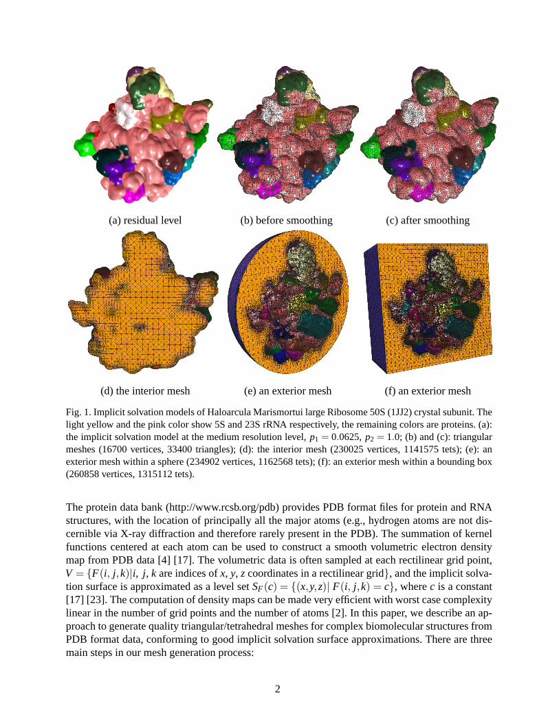
(a) residual level (b) before smoothing (c) after smoothing

(d) the interior mesh (e) an exterior mesh (f) an exterior mesh

Fig. 1. Implicit solvation models of Haloarcula Marismortui large Ribosome 50S (1JJ2) crystal subunit. Thelight yellow and the pink color show 5S and 23S rRNA respectively, the remaining colors are proteins. (a):the implicit solvation model at the medium resolution level,p1 = 0.0625,p2 = 1.0; (b) and (c): triangularmeshes (16700 vertices, 33400 triangles); (d): the interior mesh (230025 vertices, 1141575 tets); (e): anexterior mesh within a sphere (234902 vertices, 1162568 tets); (f): an exterior mesh within a bounding box(260858 vertices, 1315112 tets).

The protein data bank (http://www.rcsb.org/pdb) providesPDB format files for protein and RNAstructures, with the location of principally all the major atoms (e.g., hydrogen atoms are not dis-cernible via X-ray diffraction and therefore rarely present in the PDB). The summation of kernelfunctions centered at each atom can be used to construct a smooth volumetric electron densitymap from PDB data [4] [17]. The volumetric data is often sampled at each rectilinear grid point,V = {F(i, j,k)|i, j, k are indices ofx, y, zcoordinates in a rectilinear grid}, and the implicit solva-tion surface is approximated as a level setSF(c) = {(x,y,z)| F(i, j,k) = c}, wherec is a constant[17] [23]. The computation of density maps can be made very efficient with worst case complexitylinear in the number of grid points and the number of atoms [2]. In this paper, we describe an ap-proach to generate quality triangular/tetrahedral meshesfor complex biomolecular structures fromPDB format data, conforming to good implicit solvation surface approximations. There are threemain steps in our mesh generation process:

2

(1) Implicit Solvation Surface – A good approximation of theimplicit solvation surface is gen-erated from a smooth volumetric synthetic electron densitymap by a careful choice of theparameter of Gaussian kernel functions.

(2) Mesh Generation – The modified dual contouring method is used to generate triangular andinterior/exterior tetrahedral meshes.

(3) Quality Improvement – Geometric flows are used to improvethe quality of extracted trian-gular and tetrahedral meshes.

The summation of Gaussian kernel functions is used to construct the density map of a biomoleculeand sampled volumetric data. A smooth implicit solvation model can be constructed to approxi-mate the Lee-Richards molecular surface by using weighted Gaussian isotropic kernel functionsand a two-level clustering techniques.

The dual contouring method [19] [42] [43] is selected for mesh generation as it tends to yieldmeshes with better aspect ratio. In order to generate exterior meshes, we add a sphere or boxoutside the biomolecular surface as an outer boundary. A variant of the dual contouring methodis developed to extract interior and exterior meshes. Our tetrahedral mesh is spatially adaptiveand attempts to preserve molecular surface features while minimizing the number of elements. Anextension step is performed to generate the exterior mesh.

The extracted triangular and tetrahedral meshes cannot be directly used for finite element calcula-tions, they need to be modified and improved. Since the isosurface generated from discrete volu-metric data suffers from noise, geometric flows are used to smooth the generated surface mesheswith feature preserved. The quality of extracted surface and volume meshes is also improved.

The main contributions of this paper include: a simple and uniform treatment for approximatingimplicit solvation models, a modified adaptive surface and volume mesh extraction scheme com-bined with geometric flows and therefore yields high qualitymeshes. The generated meshes of themonomeric and tetrameric mouse acetylcholinesterase (mAChE) have been successfully used insolving the steady-state Smoluchowski equation using finite element method [36] [37] [41].

The remainder of this paper is organized as the following: Section 2 reviews related previous work.Section 3 introduces how to construct implicit solvation surface from PDB format data. Section4 explains mesh generation schemes. Section 5 discusses mesh quality improvement. Section 6presents results and conclusion.

2 Previous Work

Molecular Surface Approximation: There are three different approximations of molecular sur-faces or interfaces [31], the van der Waals surface (VWS), thesolvent-accessible surface (SAS)and the solvent-excluded surface (SES) or the Lee-Richards surface [22]. The VWS is simply theboundary of the union of balls. As introduced in [22], the SASis an inflated VWS with a probesphere. The SES is a surface inside of which the probe never intrudes.

3

According to the properties of molecular structures, Laug and Borouchaki used a combined advancing-front and generalized-Delaunay approach to mesh molecularsurfaces [21]. Algorithms were de-veloped for sampling and triangulating a smooth surface with correct topology [1]. Skin surfaces,introduced by Edelsbrunner in [9], have a rich combinational structure and are suitable for model-ing large molecules in biological computing. Cheng et. al [6]maintained an approximating trian-gulation of a deforming skin surface. Simplex subdivision schemes are used to generate tetrahedralmeshes for molecular structures in solving the Poisson-Boltzmann equation [18]. Gaussian func-tions have been used to construct density maps [4] [17] [28],from which implicit solvation modelsare approximated as an isocontour [17] [23] [14]. However, it still remains a challenging problemto generate quality triangular and tetrahedral meshes for large complicated molecular structures.

Mesh Generation: As reviewed in [30] [38], octree-based, advancing front based and Delaunaylike techniques were used for triangular and tetrahedral mesh generation. The octree techniquerecursively subdivides the cube containing the geometric model until the desired resolution isreached [33]. Advancing front methods start from a boundaryand move a front from the bound-ary towards empty space within the domain [12] [25]. Delaunay refinement is to refine trianglesor tetrahedra locally by inserting new nodes to maintain theDelaunay criterion (‘empty circum-sphere’) [8]. Sliver Exudation [7] was used to eliminate those slivers. Shewchuk [34] solved theproblem of enforcing boundary conformity by constrained Delaunay triangulation (CDT).

The predominant algorithm for isosurface extraction from volume data is Marching Cubes (MC)[26], which computes a local triangulation within each cubeto approximate the isosurface by us-ing a case table of edge intersections. MC was extended to extract tetrahedral meshes betweentwo isosurfaces [13]. A different and systematic algorithmwas proposed for interval volume tetra-hedralization [29]. By combining SurfaceNets [16] and the extended Marching Cubes algorithm[20], octree based Dual Contouring [19] generates adaptive multiresolution isosurfaces with goodaspect ratio and preserves sharp features. The dual contouring method has already been extendedto extract adaptive and quality tetrahedral meshes from volumetric imaging data [42] [43].

Quality Improvement: Algorithms for mesh improvement can be classified into threecategories[38] [30]: local coarsening/refinement by inserting/deleting points, local remeshing by face/edgeswapping and mesh smoothing by relocating vertices.

Laplacian smoothing relocates the vertex position at the average of the nodes connecting to it [10].Instead of relocating vertices based on a heuristic algorithm, the optimization technique measuresthe quality of the surrounding elements to a node and attempts to optimize it. The optimization-based smoothing yields better results while it is more expensive than Laplacian smoothing. There-fore, a combined Laplacian/Optimization-based approach was recommended [5] [11]. The Lapla-cian operator was discretized over triangular meshes [27],and geometric flows have been usedin surface and imaging processing [32] [40]. Physically-based simulations are used to repositionnodes [24]. Anisotropic meshes are obtained from bubble equilibrium [35].

4

3 Implicit Solvation Surface from volumetric Density Maps

We extract the implicit solvation surface (molecular surface) as a level set of the volumetric syn-thetic electron density maps. The implicit solvation surface is chosen to be a good approximationof the Lee-Richards molecular surface [22] by choosing an appropriate parameter of the Gaussiankernel functions.

3.1 Gaussian Density Map

As used for Poisson-Boltzmann electrostatics calculationsin [18], a characteristic functionf (x) isselected to represent an ‘inflated’ van der Waals-based accessibility

f (x) =

1, if ‖x−xi‖ < r i +σ for i = 1, . . . ,N,

0, otherwise,(1)

where (xi, ri) are the centers and radii of the N atoms in the biomolecule, and σ is the radiusof the diffusing species, here we chooseσ = 2 [37]. Whenσ = 0, the VWS is constructed. Thefunction f (x) provides a grid-based volumetric data which can be isocontoured at the isovalue 0.5to represent the SAS. Fig. 16(a) shows one constructed geometric model of mAChE.

Molecules are often modelled as the union of hard spheresSi (atoms). The surface, denoted asM0,of a molecule is therefore described as the boundary of the union of balls. To have the blurringeffect at the intersection parts of atoms, the molecular surface is approximated by an isocontour[4]:

M :={

x∈ R3 : G(x) = 1

}

(2)

with

G(x) =N

∑i=1

eBi

(

‖x−xi‖2

r2i−1

)

, (3)

where (xi , ri) are the center and radius of theith atom in the biomolecule, andBi < 0 is called‘decay rate’, which controls the blurring effect. Note thatBi must be negative to ensure that thedensity function goes to zero as‖ x− xi ‖ goes to infinity. In order to make the distance betweenM andM0 as uniformly as possible, we take

C = Bi/r2i , (4)

whereC < 0 is a given constant. NowG(x) becomes

5

G(x,C) =N

∑i=1

eC(‖x−xi‖2−r2

i ). (5)

The various presentationM(Ci) = {x ∈ R3 : G(x,Ci) = 1} of the molecular surface is therefore

achieved by takingC = C1, . . . ,Cl .

As shown in Fig. 2, the different effects ofC and constantBi(= B) are studied in a two-spheresystem, one is centering at (0, 0, 0) with the radius of 1.0, the other one is at (2.8, 0, 0) with theradius of 2.0. It could be observed that

Fig. 2. Implicit Solvation models by choosing various C in (a) and Bi in (b). Yellow balls are two inputatoms. The correspondence between C/Bi values and these models are shown in Table 1.

Table 1: C/Bi and Implicit Solvation Models in Fig. 2

Red Green Magenta Blue

Fig.2(a) C = -0.125 C = -0.25 C = -0.5 C = -1.0

Fig.2(b) Bi= -0.125 Bi= -0.25 Bi= -0.5 Bi= -1.0

• C leads to more uniform inflation thanBi.• Small balls have more inflation than big ones.• Large error happens around the intersection region, and error reduces gradually away from it.• LargerC andBi lead to more inflation. For the same C andBi value, e.g., -0.125,Bi tends to

introduce more inflation.

Fig. 3 shows implicit solvation models of Ribosome 30S. Compared with Fig. 3(a), proteins inflatemuch more seriously in Fig. 3(e). rRNA in Fig. 3(c) and (f) looks similar, but proteins in Fig. 3(f)look a little more inflated than Fig. 3(b). rRNA in Fig. 3(d) and(g) looks similar too, but proteinsin Fig. 3(g) are close to proteins in Fig. 3(c).

6

(a) C = -0.03125 (b) C = -0.125 (c) C = -0.25 (d) C = -0.5

(e) B = -0.03125 (f) B = -0.125 (g) B = -0.5Fig. 3. Implicit solvation models of Thermus Thermophilus small Ribosome 30S (1J5E) crystal subunit forvarious Gaussian kernel parameters. The pink color shows 16S rRNA and the remaining colors are proteins.

3.2 Multi-Level Gaussian Density Map

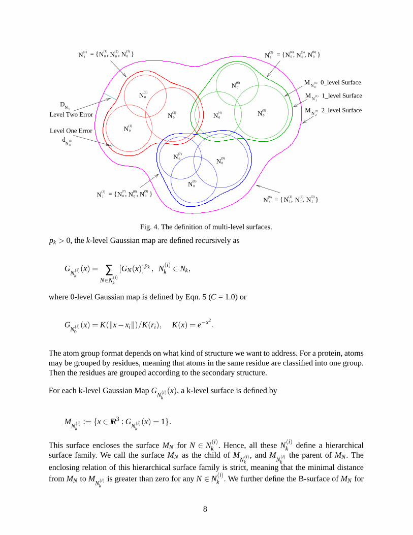
In order to model different level structures, we introduce multi-level Gaussian map. First let us

introduce some notations as shown in Fig. 4. LetN0 = {N(0)0 , · · · ,N(n)

0 } denote the index set of all

the atoms withN(i)0 = {i}. SupposeN0 is grouped into several subsetsN(i)

1 , i = 1,2, · · · ,n1, suchthat

n1⋃

i=1

N(i)1 = N0, N(i)

1

⋂

1≤i 6= j≤n1

N( j)1 = φ. (6)

The setN1 := {N(i)1 }n1

i=1, whose elements are also sets, may be further grouped into some subsets

N(i)2 , i = 1,2, · · · ,n2, such that

n2⋃

i=1

N(i)2 = N1, N(i)

2

⋂

1≤i 6= j≤n2

N( j)2 = φ. (7)

The collection of{N(i)2 }n2

i=1 is denoted byN2. This hierarchical grouping process could be repeatedseveral times according to the nature of the molecular complex considered. In practical, two or

three iterations may be enough. By using these setsN(i)k and a given sequence{pk} of p with

7

N

D1N

(1)

0N

0

N

M1N

0_level SurfaceM (5)

d

(1)N2

(0)N

0

(9)

1 = { , , }1

(3)N1

(2)N

2

(0) 2_level Surface

(1) 1_level Surface

Level Two Error

Level One Error

M

N

(8)N

0

(9)N

0

(6)

0

NN0

(1)

0

(7)N

N

N

0

(3)N

N0

(1)

(2)0

(5)N

0

(4)N0

(2)

N = { , , }

0

(6)N0

(5)

(3)

0

(8)N0

(7)N1

N(1)

N = { , , }0

(3)N01 0

(4)N1

(2)N = { , , }

Fig. 4. The definition of multi-level surfaces.

pk > 0, thek-level Gaussian map are defined recursively as

GN(i)

k(x) = ∑

N∈N(i)k

[GN(x)]pk , N(i)k ∈ Nk,

where 0-level Gaussian map is defined by Eqn. 5 (C = 1.0) or

GN(i)

0(x) = K(‖x−xi‖)/K(r i), K(x) = e−x2

.

The atom group format depends on what kind of structure we want to address. For a protein, atomsmay be grouped by residues, meaning that atoms in the same residue are classified into one group.Then the residues are grouped according to the secondary structure.

For each k-level Gaussian MapGN(i)

k(x), a k-level surface is defined by

MN(i)

k:= {x∈ IR3 : G

N(i)k

(x) = 1}.

This surface encloses the surfaceMN for N ∈ N(i)k . Hence, all theseN(i)

k define a hierarchicalsurface family. We call the surfaceMN as the child ofM

N(i)k

, andMN(i)

kthe parent ofMN. The

enclosing relation of this hierarchical surface family is strict, meaning that the minimal distance

from MN to MN(i)

kis greater than zero for anyN ∈ N(i)

k . We further define the B-surface ofMN for

8

(a) low resolution (b) residual level (c) atomic levelFig. 5. Implicit solvation models of Haloarcula Marismortui large Ribosome 50S (1JJ2) crystal subunit. (a)p1 = 0.03125; (b)p1 = 0.125; (c)p1 = 0.5. p2 = 1.0. The light yellow and the pink color show 5S and 23SrRNA respectively, the remaining colors are proteins.

all N ∈ N(i)k as

SN(i)

k= Bd

(⋃

N∈N(i)k

{x∈ IR3 : GN(x) ≤ 1})

,

where Bd() denotes the boundary of a region inIR3. Note thatSN(i)

kis enclosed strictly byM

N(i)k

.

The aim to introduce multi-level Gaussian map is to address the structure of molecules at a cer-tain level. For instance, at the residual level of a protein,we regard each residue as one unit andtherefore the residue is modelled as one structure. The sub-structures of the residue (atoms), arenot modelled individually. Similarly, at the secondary level, a group of residues is regraded as oneunit while the residues are not regarded as individual structures. The goal of addressing certainlevel structure and un-addressing the higher level ones is achieved by the properly selection of theparameterpk in the multi-level Gaussian map. Basically, largerpk should be chosen to addressk-level structure and smallerpk−1 is used to un-address(k−1)-level structures.

Considering three levels of structures, including the atomic, the residual and the second levels,we can construct three level Gaussian map with givenp1, p2 and p3. To address the secondarystructure, we need to choosep3 larger andp2 smaller, whilep1 have less influence to the secondarystructure. Therefore, we consider only two-level Gaussianmap instead of three: Level one is theresidual level, Level two is the low level. In this paper, we only consider two-level Gaussian map.

In implicit solvation modeling, various models are constructed by choosing differentp1 ∈ (0,∞)and p2 ∈ (0,∞) in the Gaussian map. To make the constructed model correspond to a certainlevel, p1 and p2 need to be selected properly. For a fixed level, the structureat this level shouldbe distinguishable, while the structure at a higher level may not be presented remarkably. Forinstance, at the residual level, the chain structure of residuals should be observed, while atomsmay not be distinguished clearly. Fig. 5 shows constructed models of Ribosome 50S at the lowresolution, residual and atomic levels.

9

3.3 Surface Point Classification and Parameterization

The adopted multi-level Gaussian map addresses certain substructures, which are visually distin-guishable. To enhance the contrast, certain color maps may be used to paint the substructures.Therefore, a classification of the surface points is required. Basically, the problem is: for each

point p∈ MN( j)

kwe need to classify this point by its child surfacesMN, N ∈ N( j)

k . Point p∈ MN( j)

kbelongs toMN if and only if

GN(p) ≥ GN(p) ∀N ∈ N( j)k N 6= N. (8)

Such a classification is unique for point which makes the inequality above hold strictly, otherwise,it is not unique. According to this classification of surface, M

N( j)k

is partitioned into patches, each

of them belongs to one child surface. We denote the patch belonging toMN by MN( j)

k ,N.

The surfaceMN( j)

kcould be classified according to zero level surfaces. That is, the pointp∈ M

N( j)k

belongs toSN(i)

0if and only if

GN(i)

0(p) ≥ GNk

0(p) ∀ i 6= k. (9)

Let xi andr i be the center and radius ofSi . Then

P(p) := xi +r i(p−xi)

‖p−xi‖(10)

is the nearest point fromp to SN(i)

0. Equation (10) establishes a mapping from a patch of surface

MN( j)

k, which belongs to sphereSi, to a patch of sphereSi . It follows from [3] that this patch of

sphere could be represented exactly by a NURB patch over a(u,v) domain, with trimming curvesas the boundaries of the patch. Therefore, the mapping (10) leads to a piecewise parameterizationof the surfaceM

N( j)k

.

3.4 Error Computation

In order to obtain the tight enclosing surface for the first level, we need to compute the minimal

distance fromMN, N ∈ N(i)1 to its parent surfaceM

N(i)1

. On the other hand, in order to have an error

controlled approximation of the second level surface, we need to compute the maximal error from

MN, N ∈ N(i)2 to its parent surfaceM

N(i)2

. Hence, we need to consider the error computation for two

levels of surfaces. The error computations are based on a point projection algorithm.

Given the surfaceMN, a pointq /∈ MN and a unit directionn, the point projection algorithm in thefollowing computes a nearby intersection pointp of the lineq+ tn (t ∈ (−∞,∞)) with the surfaceMN.

10

Algorithm 3.4.1 (Point Projection).

(1) Compute an interval[a,b] for t, on whichGN(q+ tn)−1 changes sign once. This is achievedby a linear search step in a certain range[A,B]. If (∇GN(q))Tn[GN(q)−1] < 0, search inndirection, otherwise in−n direction. If such an interval could not be found, the project pointdoes not exist and return a failure signal. After the interval is determined, sett0 = a+b

2 andk = 0.

(2) Computetk+1 by the Newton iteration method

tk+1 = tk−GN(q+ tkn)

nT∇GN(q+ tkn). (11)

If tk+1 /∈ (a,b), replacetk+1 by a+b2 .

(3) Replace the interval[a,b] by [a, tk+1] if GN(q+tn)−1 changes sign over[a, tk+1], and replace[a,b] by [tk+1,b] otherwise.

(4) If |b− a| < ε (ε is a given error tolerance, we take it to be10−4), stop the iteration andp = q+ tk+1n is the projection point, otherwise, setk = k+1 and go back to step 2.

We specify the searching range[A,B] in step 1 of the algorithm to be[−4,4], since the atomdiameters are around 4. Errors beyond that are not considered here. If the projection exists, thenthe projection pointp of pointq on the surfaceMN in the directionn is denoted byPMN(q,n).

3.4.1 Minimal Error of Level One Surface

Now we assumek = 1, then the child surfaces are atoms. LetN = { j} ∈ N(i)1 , the minimal error

from MN = SN to MN(i)

1is defined by

dN := minp∈M

N(i)1 ,N

‖p−x j‖− r j , j ∈ N.

Let q = x j + r jp−x j

‖p−x j‖, thenq is on the sphereSN andp is the projection ofq to the surfaceM

N(i)1

in the spherical normal directionn(q). That is,p = PMN

(i)1

(q,n(q)). Hence in order to computedN,

we need to computePMN

(i)1

(q,n(q)) for q∈ SN.

Now we consider the computation of the minimal distance fromMN to MN(i)

1, where N ∈ N(i)

1 .

First we assume that each atom (sphere) is uniformly sampledwith m vertices. This sampling isachieved by translating a triangulated unit sphere to each of the atom center and re-scaling it to theatom size. We obtain the unit sphere triangulation from [39]. For each vertexq on the triangulatedatom surfaceMN, PM

N(i)1

(q,n(q)) is computed using thepoint projectionalgorithm, wheren(q) is

the spherical normal atq.

Algorithm 3.4.2 (Minimal Error computation).

11

SetdN = 4.

for each triangle vertexq∈ SN ∩SN0 do{

computePMN1(q,n(q)), and then compute

dN = min{dN,‖PMN1(q,n(q))−x j‖− r j},

if PMN1(q,n(q)) ∈ MN1,N.

(12)

}

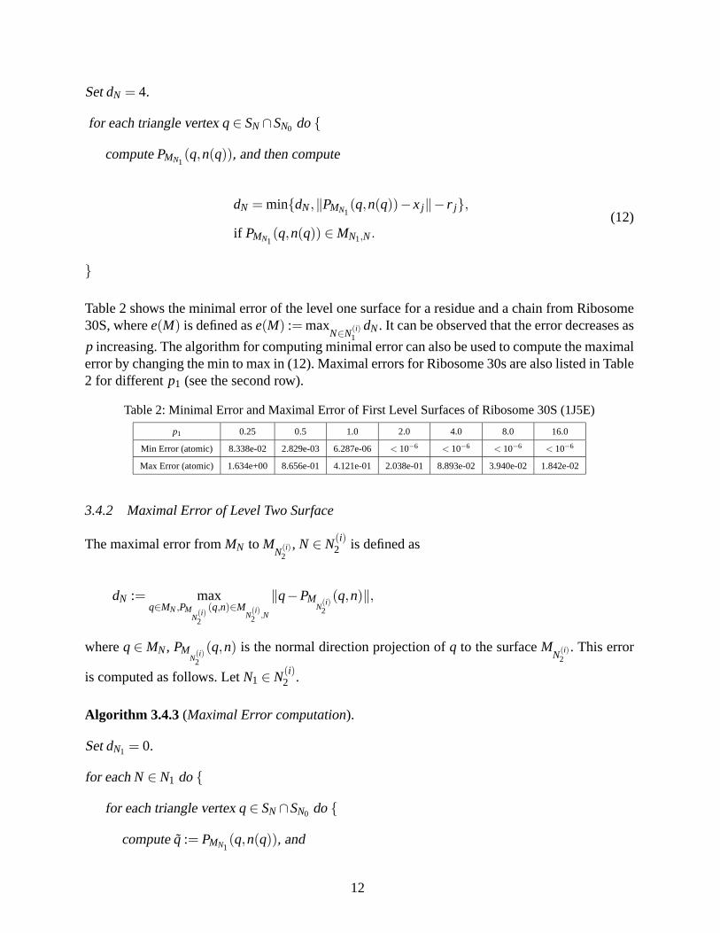
Table 2 shows the minimal error of the level one surface for a residue and a chain from Ribosome30S, wheree(M) is defined ase(M) := max

N∈N(i)1

dN. It can be observed that the error decreases as

p increasing. The algorithm for computing minimal error can also be used to compute the maximalerror by changing the min to max in (12). Maximal errors for Ribosome 30s are also listed in Table2 for differentp1 (see the second row).

Table 2: Minimal Error and Maximal Error of First Level Surfaces of Ribosome 30S (1J5E)

p1 0.25 0.5 1.0 2.0 4.0 8.0 16.0

Min Error (atomic) 8.338e-02 2.829e-03 6.287e-06 < 10−6 < 10−6 < 10−6 < 10−6

Max Error (atomic) 1.634e+00 8.656e-01 4.121e-01 2.038e-01 8.893e-02 3.940e-02 1.842e-02

3.4.2 Maximal Error of Level Two Surface

The maximal error fromMN to MN(i)

2, N ∈ N(i)

2 is defined as

dN := maxq∈MN,PM

N(i)2

(q,n)∈MN

(i)2 ,N

‖q−PMN

(i)2

(q,n)‖,

whereq∈ MN, PMN

(i)2

(q,n) is the normal direction projection ofq to the surfaceMN(i)

2. This error

is computed as follows. LetN1 ∈ N(i)2 .

Algorithm 3.4.3 (Maximal Error computation).

SetdN1 = 0.

for eachN ∈ N1 do{

for each triangle vertexq∈ SN ∩SN0 do{

computeq := PMN1(q,n(q)), and

12

computePMN

(i)2

(q,n(q)) if q∈ MN1,N

and then compute

dN1 = max{dN1,‖PMN1(q,n(q))−PM

N(i)2

(q,n(q))‖

if PMN

(i)2

(q,n(q)) ∈ MN(i)

2 ,N1.

}

}

Again, the projection points ˜q = PMN1(q,n(q)) andPM

N(i)2

(q,n(q)) are computed by the point pro-

jection algorithm, where the searching range[A,B] is set to be[0,4], since we knowMN(i)

2enclosing

MN and we are not interested in the errors that are larger than 4.

The first row of Table 3 shows the maximal errors of the second level (residual level) surfaces forribosome 30s, wherep1 is chosen to be 0.5, p2 = 0.25,0.5,1.0, · · · ,16. The second row lists themaximal errors of the second level (low level) surfaces for the samep1 andp2. The results showthat the errors decrease in approximately linear rate asp2 increases.

Table 3: Maximal Error of Second Level Surfaces of Ribosome 30S (1J5E)

p2 0.25 0.5 1.0 2.0 4.0 8.0 16.0

Max Error (residual) 3.923e+00 2.124e+00 6.832e-01 3.240e-01 1.550e-01 7.794e-02 3.278e-02

Max Error (low) 9.899e+00 7.695e+00 8.045e-01 2.365e-01 1.390e-01 6.113e-02 2.653e-02

3.5 Good Approximations of Molecular Surfaces

We have discussed that it is sufficient to consider two-levelGaussian map. To address certainstructures,p1 is taken to be a small value to blur the higher level details,p2 is chosen to be largerto enhance the feature of the current level structure. As we have shown in the last section, a smallerp1 leads to a larger error for the level one surface, and a largerp2 leads to a smaller error for thesecond level surface. Therefore, our strategy for obtaining tight enclosing surface is to remove thelevel one error and ignore the error of the second level.

The main idea to obtain the tight level one enclosing surfaceMN(1)

1is to reduce the radii of the

atoms, such thatMN(i)

1touches the original atoms (see Fig. 6). Supposey ∈ M

N(i)1

is the nearest

point to thej-th atom, j ∈ N(i)1 , and the distance fromy to the atom isd j . Then we have

∑l∈N(i)

1 ,l 6= j

[K(‖y−xl‖)/K(r l )]p1 +[K(‖y−x j‖)/K(r j)]

p1 = 1. (13)

13

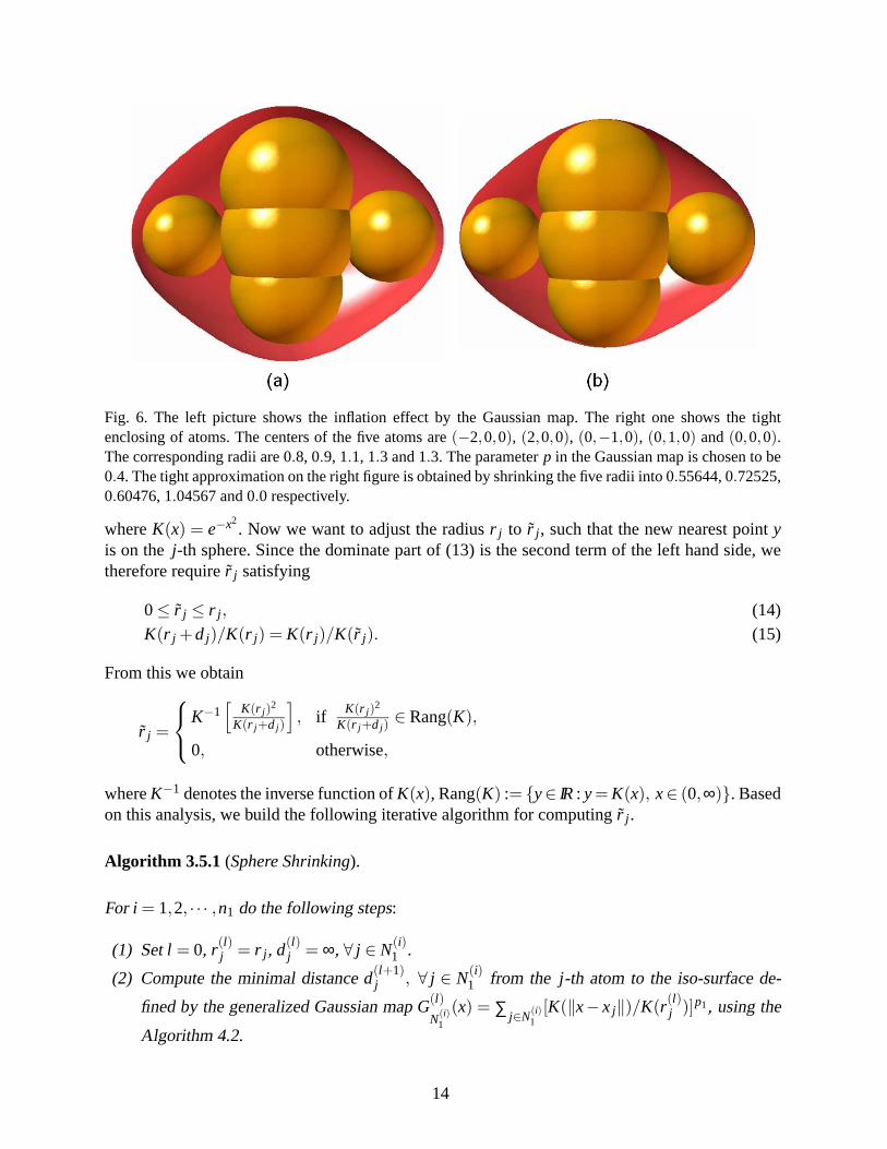
Fig. 6. The left picture shows the inflation effect by the Gaussian map. Theright one shows the tightenclosing of atoms. The centers of the five atoms are(−2,0,0), (2,0,0), (0,−1,0), (0,1,0) and(0,0,0).The corresponding radii are 0.8, 0.9, 1.1, 1.3 and 1.3. The parameterp in the Gaussian map is chosen to be0.4. The tight approximation on the right figure is obtained by shrinking the fiveradii into 0.55644, 0.72525,0.60476, 1.04567 and 0.0 respectively.

whereK(x) = e−x2. Now we want to adjust the radiusr j to r j , such that the new nearest pointy

is on the j-th sphere. Since the dominate part of (13) is the second termof the left hand side, wetherefore require ˜r j satisfying

0≤ r j ≤ r j , (14)K(r j +d j)/K(r j) = K(r j)/K(r j). (15)

From this we obtain

r j =

K−1[

K(r j )2

K(r j+d j )

]

, if K(r j)2

K(r j+d j )∈ Rang(K),

0, otherwise,

whereK−1 denotes the inverse function ofK(x), Rang(K) := {y∈ IR : y= K(x), x∈ (0,∞)}. Basedon this analysis, we build the following iterative algorithm for computing ˜r j .

Algorithm 3.5.1 (Sphere Shrinking).

For i = 1,2, · · · ,n1 do the following steps:

(1) Setl = 0, r(l)j = r j , d(l)

j = ∞, ∀ j ∈ N(i)1 .

(2) Compute the minimal distanced(l+1)j , ∀ j ∈ N(i)

1 from the j-th atom to the iso-surface de-

fined by the generalized Gaussian mapG(l)

N(i)1

(x) = ∑j∈N(i)

1[K(‖x− x j‖)/K(r(l)

j )]p1, using the

Algorithm 4.2.

14

Fig. 7. Different effects of changingp2 and tight/non-tight approximations for three amino acids (ASN,THR and TYR) which consist of 49 atoms. The surface (b), (c) and (d)are the same as outer surfaces of (e),(f) and (g) respectively. The inner surface of (e), (f) and (g) is the hard sphere model of three residues. (a)shows the atomic level approximation of the hard sphere model, wherep1 = 5.0, p2 = 1.0; (b), (e), (c) and(f) show the tight approximation of the residual level withp1 = 0.4. But differentp2 are used. We choosep2 = 2.0 for (b) p2 = 0.5 for (c). It could be observed that largerp2 leads to closer approximation. (d) and(g) show non-tight approximations using the samep1 andp2 as (c) and (f). Comparing with (f), even largererror is observed in (g).

(3) Compute

r(l+1)j =

K−1

[

K(r j )K(r(l)j )

K(r j+d(l)j )

]

, ifK(r j )K(r(l)

j )

K(r j+d(l)j )

∈ Rang(K),

0, otherwise.

(4) If maxj∈N(i)

1|d(l)

j − d(l+1)j | < ε (we takeε = 10−4), terminate thel loop andr(l+1)

j are the

required results. Otherwise, setl = l +1 and go back to step 2.

Remark: The conditionK(r j )K(r(l)

j )

K(r j+d(l)j )

∈ Rang(K) may lead to some of the atoms locating in the deep

inside of the molecule are not touchable. Figure 6 shows thatthe circle at the origin is not touched.

The experiments show the sphere shrinking algorithm converges in a linear rate. Table 4 lists the

errore(l)max= max

j∈N(i)1|d(l)

j | for 20 amino acids withp1 = 0.4. These amino acids are taken from

the protein mAChE. We notice that the shape of different copies of one amino acids will differ.Currently, we are studying theoretically the convergence ofthe algorithm.

15

Table 4: Errorse(l)max for 20 amino acids andp1 = 0.4

l ALA ARG ASN ASP CYS GLN GLU GLY HSD ILE

0 5.13e-01 6.97e-01 5.99e-01 6.23e-01 5.36e-01 6.26e-01 7.06e-01 4.34e-01 7.36e-01 6.00e-01

2 6.22e-02 1.37e-01 2.66e-01 6.75e-02 5.86e-02 1.16e-01 7.78e-02 5.33e-02 7.20e-02 5.62e-02

4 2.80e-03 3.79e-02 5.83e-02 1.50e-03 6.82e-04 1.76e-03 4.57e-04 1.90e-02 1.45e-02 2.73e-03

6 5.76e-04 2.30e-02 1.83e-04 4.93e-04 1.81e-04 4.51e-04 1.38e-04 8.62e-05 5.30e-03 5.60e-04

8 1.30e-04 6.95e-04 6.06e-05 1.64e-04 4.97e-05 1.74e-04 4.26e-05 6.31e-06 2.20e-03 1.25e-04

10 3.14e-05 2.18e-04 2.22e-05 5.59e-05 1.39e-05 7.84e-05 1.32e-05 7.16e-07 9.94e-04 3.11e-05

l LEU LYS MET PHE PRO SER THR TRP TYR VAL

0 8.48e-01 8.62e-01 6.08e-01 6.14e-01 7.98e-01 9.63e-01 1.06e-00 6.01e-01 6.10e-01 7.07e-01

2 6.51e-02 3.96e-01 1.13e-01 8.94e-02 2.06e-03 8.81e-02 3.06e-02 9.17e-02 6.03e-02 2.86e-02

4 5.72e-03 1.54e-03 7.78e-03 6.50e-03 3.62e-04 5.28e-04 6.63e-03 1.49e-02 4.25e-02 5.76e-03

6 1.27e-03 5.18e-04 2.25e-03 1.90e-03 9.12e-05 1.19e-04 1.68e-03 6.42e-03 1.69e-03 1.36e-03

8 3.03e-04 1.77e-04 6.77e-04 7.13e-04 2.35e-05 2.66e-05 4.67e-04 2.90e-03 6.93e-04 3.56e-04

10 7.52e-05 6.23e-05 2.09e-04 3.02e-04 6.26e-06 5.88e-06 1.36e-04 1.56e-03 3.52e-04 9.78e-05

Fig. 8. Multi-resolution models of Ribosome 30S. (a) - Ribosome 30S at the low level with p1 = 0.0625,p2 = 1.0 in multi-level Gaussian map. Ribosome 30S contains 22 chains and each of them is painted in adifferent color. The pink color shows 16S rRNA and the remaining colorsare proteins. The blue box showsone protein (Chain B). (b) - Chain B at the residual level withp1 = 0.4, p2 = 5.0. It consists of 234 residues.(c) - Chain B at the atomic level withp1 = 5.0, p2 = 1.0. It consists of 1900 atoms.

Fig. 7 shows multi-resolution models of the amino acid ASN, THR and TYR with variousp1

and p2. Fig. 7(a) shows an atomic level model, Fig. 7(a∼g) are residual level models. It can beobserved that when the samep1 is selected, smallerp2 leads to fatter surfaces. Compared withFig. 7(g), Fig. 7(f) is more tight.

Fig. 8 shows multi-resolution models of Ribosome 30S. Fig. 8(a) is a low level model, the pinkcolor shows 16S rRNA and the remaining colors are proteins. One protein (Chain B) is separatedfrom the whole structure. The residual level model can be constructed by selecting smallp1 and

16

largep2 as shown in Fig. 8(b), and the atomic level model is constructed by selecting largep1 andsmall p2 as shown in Fig. 8(c).

4 Mesh Generation

There are two main methods for contouring scalar fields, primal contouring [26] and dual con-touring [19]. Both of them can be extended to tetrahedral meshgeneration. The dual contouringmethod [42] [43] is often the method of choice as it tends to yield meshes with better aspect ratio.

4.1 Triangular Meshing

Dual contouring [19] uses an octree data structure, and analyzes those edges that have endpointslying on different sides of the isosurface, calledsign change edges. The mesh adaptivity is de-termined during a top-down octree construction. Each sign change edge is shared by either four(uniform case) or three (adaptive case) cells, and one minimizer point is calculated for each ofthem by minimizing a predefined Quadratic Error Function (QEF) [15]:

QEF[x] = ∑i

[ni · (x− pi)]2 , (16)

wherepi, ni represent the position and unit normal vectors of the intersection point respectively.For each sign change edge, a quad or triangle is constructed by connecting the minimizers. Thesequads and triangles provide a ‘dual’ approximation of the isosurface.

A recursive cell subdivision process was used to preserve the correct topology [43] of the iso-surface. During the cell subdivision, the function value ateach newly inserted grid point can beexactly calculated since we know the function (Gaussian functions, Eqn. (5)). Additionally, wecan generate a more accurate triangular mesh by projecting each generated minimizer point ontothe isosurface (Eqn. (2)).

4.2 Tetrahedral Meshing

The dual contouring method has already been extended to extract tetrahedral meshes from volu-metric scalar fields [42] [43]. The cells containing the isosurface are called boundary cells, and theinterior cells are those cells whose eight vertices are inside the isosurface. In the tetrahedral meshextraction process, all the boundary cells and the interiorcells need to be analyzed in the octreedata structure. There are two kinds of edges in boundary cells, one is a sign change edge, the otheris an interior edge. Interior cells only have interior edges. In [42] [43], interior edges and interiorfaces in boundary cells are dealt with in a special way, and the volume inside boundary cells istetrahedralized. For interior cells, we only need to split them into tetrahedra.

17

(a) (b) (c)

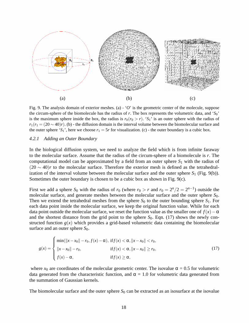
Fig. 9. The analysis domain of exterior meshes. (a) - ‘O’ is the geometric center of the molecule, supposethe circum-sphere of the biomolecule has the radius ofr. The box represents the volumetric data, and ‘S0’is the maximum sphere inside the box, the radius isr0(r0 > r). ‘S1’ is an outer sphere with the radius ofr1(r1 = (20∼ 40)r). (b) - the diffusion domain is the interval volume between the biomolecular surface andthe outer sphere ‘S1’, here we chooser1 = 5r for visualization. (c) - the outer boundary is a cubic box.

4.2.1 Adding an Outer Boundary

In the biological diffusion system, we need to analyze the field which is from infinite farawayto the molecular surface. Assume that the radius of the circum-sphere of a biomolecule isr. Thecomputational model can be approximated by a field from an outer sphereS1 with the radius of(20∼ 40)r to the molecular surface. Therefore the exterior mesh is defined as the tetrahedral-ization of the interval volume between the molecular surface and the outer sphereS1 (Fig. 9(b)).Sometimes the outer boundary is chosen to be a cubic box as shown in Fig. 9(c).

First we add a sphereS0 with the radius ofr0 (wherer0 > r andr0 = 2n/2 = 2n−1) outside themolecular surface, and generate meshes between the molecular surface and the outer sphereS0.Then we extend the tetrahedral meshes from the sphereS0 to the outer bounding sphereS1. Foreach data point inside the molecular surface, we keep the original function value. While for eachdata point outside the molecular surface, we reset the function value as the smaller one off (x)−αand the shortest distance from the grid point to the sphereS0. Eqn. (17) shows the newly con-structed functiong(x) which provides a grid-based volumetric data containing thebiomolecularsurface and an outer sphereS0.

g(x) =

min(‖x−x0‖− r0, f (x)−α), if f (x) < α,‖x−x0‖ < r0,

‖x−x0‖− r0, if f (x) < α,‖x−x0‖ ≥ r0,

f (x)−α, if f (x) ≥ α,

(17)

wherex0 are coordinates of the molecular geometric center. The isovalueα = 0.5 for volumetricdata generated from the characteristic function, andα = 1.0 for volumetric data generated fromthe summation of Gaussian kernels.

The biomolecular surface and the outer sphereS0 can be extracted as an isosurface at the isovalue

18

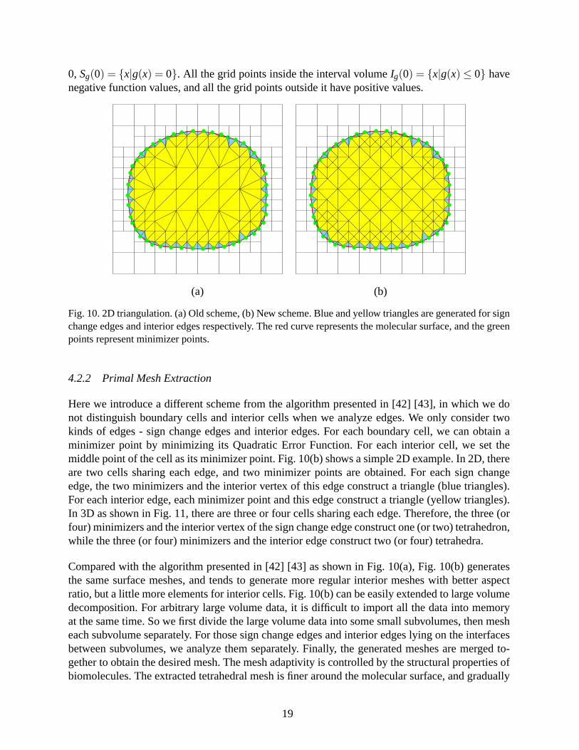
0, Sg(0) = {x|g(x) = 0}. All the grid points inside the interval volumeIg(0) = {x|g(x) ≤ 0} havenegative function values, and all the grid points outside ithave positive values.

(a) (b)

Fig. 10. 2D triangulation. (a) Old scheme, (b) New scheme. Blue and yellow triangles are generated for signchange edges and interior edges respectively. The red curve represents the molecular surface, and the greenpoints represent minimizer points.

4.2.2 Primal Mesh Extraction

Here we introduce a different scheme from the algorithm presented in [42] [43], in which we donot distinguish boundary cells and interior cells when we analyze edges. We only consider twokinds of edges - sign change edges and interior edges. For each boundary cell, we can obtain aminimizer point by minimizing its Quadratic Error Function. For each interior cell, we set themiddle point of the cell as its minimizer point. Fig. 10(b) shows a simple 2D example. In 2D, thereare two cells sharing each edge, and two minimizer points areobtained. For each sign changeedge, the two minimizers and the interior vertex of this edgeconstruct a triangle (blue triangles).For each interior edge, each minimizer point and this edge construct a triangle (yellow triangles).In 3D as shown in Fig. 11, there are three or four cells sharingeach edge. Therefore, the three (orfour) minimizers and the interior vertex of the sign change edge construct one (or two) tetrahedron,while the three (or four) minimizers and the interior edge construct two (or four) tetrahedra.

Compared with the algorithm presented in [42] [43] as shown inFig. 10(a), Fig. 10(b) generatesthe same surface meshes, and tends to generate more regular interior meshes with better aspectratio, but a little more elements for interior cells. Fig. 10(b) can be easily extended to large volumedecomposition. For arbitrary large volume data, it is difficult to import all the data into memoryat the same time. So we first divide the large volume data into some small subvolumes, then mesheach subvolume separately. For those sign change edges and interior edges lying on the interfacesbetween subvolumes, we analyze them separately. Finally, the generated meshes are merged to-gether to obtain the desired mesh. The mesh adaptivity is controlled by the structural properties ofbiomolecules. The extracted tetrahedral mesh is finer around the molecular surface, and gradually

19

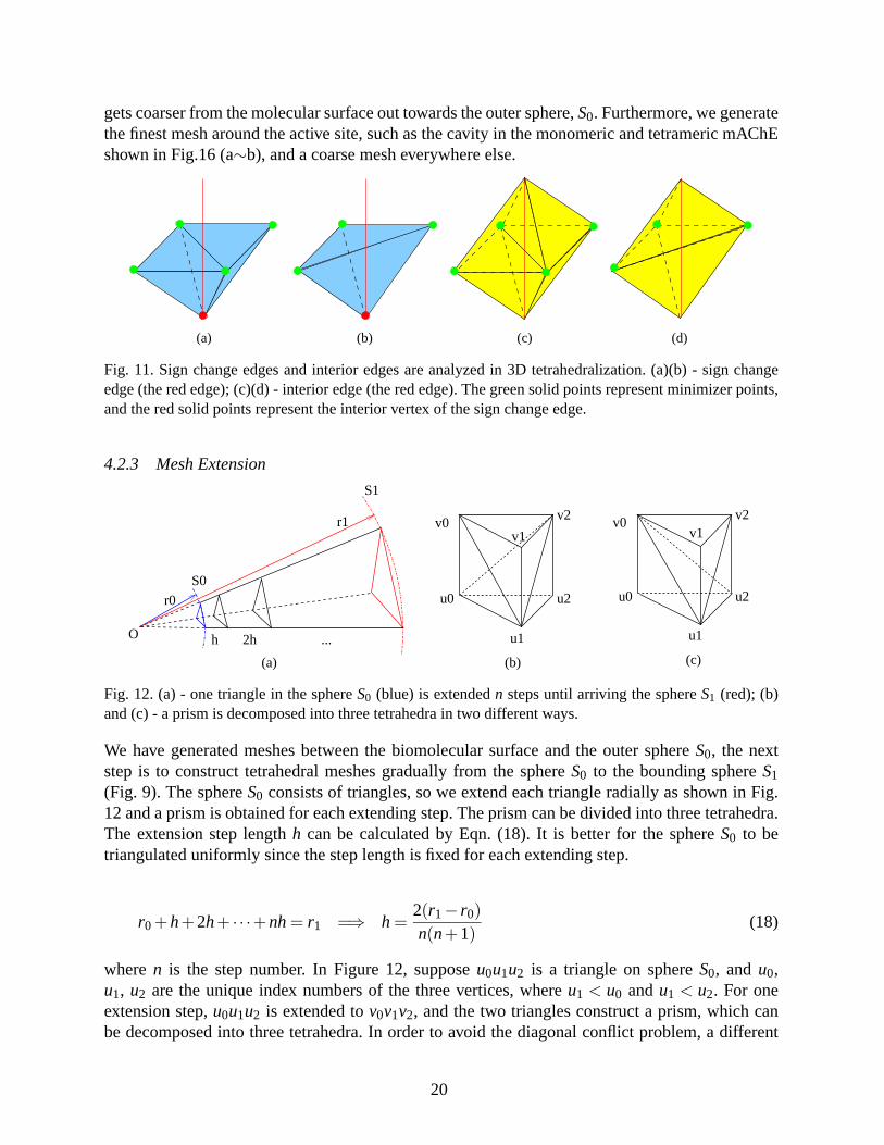
gets coarser from the molecular surface out towards the outer sphere,S0. Furthermore, we generatethe finest mesh around the active site, such as the cavity in the monomeric and tetrameric mAChEshown in Fig.16 (a∼b), and a coarse mesh everywhere else.

(b) (c) (d)(a)

Fig. 11. Sign change edges and interior edges are analyzed in 3D tetrahedralization. (a)(b) - sign changeedge (the red edge); (c)(d) - interior edge (the red edge). The green solid points represent minimizer points,and the red solid points represent the interior vertex of the sign change edge.

4.2.3 Mesh Extension

...h

r0

O

(b)

u0

2h

r1

S0

v2v0

u2

(a)

v1v1

S1

v0

u1

(c)

u0

u1

u2

v2

Fig. 12. (a) - one triangle in the sphereS0 (blue) is extendedn steps until arriving the sphereS1 (red); (b)and (c) - a prism is decomposed into three tetrahedra in two different ways.

We have generated meshes between the biomolecular surface and the outer sphereS0, the nextstep is to construct tetrahedral meshes gradually from the sphereS0 to the bounding sphereS1

(Fig. 9). The sphereS0 consists of triangles, so we extend each triangle radially as shown in Fig.12 and a prism is obtained for each extending step. The prism can be divided into three tetrahedra.The extension step lengthh can be calculated by Eqn. (18). It is better for the sphereS0 to betriangulated uniformly since the step length is fixed for each extending step.

r0 +h+2h+ · · ·+nh= r1 =⇒ h =2(r1− r0)

n(n+1)(18)

wheren is the step number. In Figure 12, supposeu0u1u2 is a triangle on sphereS0, and u0,u1, u2 are the unique index numbers of the three vertices, whereu1 < u0 andu1 < u2. For oneextension step,u0u1u2 is extended tov0v1v2, and the two triangles construct a prism, which canbe decomposed into three tetrahedra. In order to avoid the diagonal conflict problem, a different

20

decomposition method (Fig. 12(b∼c)) is chosen based on the index number of the three vertices.If u0 < u2, then we choose Fig. 12(b) to split the prism into three tetrahedra. Ifu2 < u0, then Fig.12(c) is selected

Assume there arem triangles on the sphereS0, which is extendedn steps to arrive the sphereS1.m prisms or 3m tetrahedra are generated in each extending step, and a totalof 3mn tetrahedra areconstructed in the extension process. Therefore, it is better to keep coarse and uniform triangularmesh on the sphereS0.

5 Quality Improvement

In general, the molecular surface generated by iscontouring the Gaussian density function or thecharacteristic function is bumpy. This is because the volume data could not be sufficiently fine dueto the capacity limit of the computer, and is not smooth enough, especially for the data generatedfrom the characteristic function. The error of the isosurface from the characteristic function couldbe as large as half of the grid size since the characteristic function generates binary volumetricdata, and could be very large relative to the atom size. Therefore, a post-processing step for theextracted isosurface is necessary. There are three tasks for the mesh quality improvement:

(1) Denoising the surface mesh (vertex adjustment in the normal direction).(2) Improving the aspect ratio of the surface mesh (vertex adjustment in the tangent direction).(3) Improving the aspect ratio of the volumetric mesh (vertex adjustment inside the volume).

We use geometric partial differential equations (PDEs) to handle the first two problems. GeometricPDEs, such as the mean curvature flow, the surface diffusion flow and Willmore flow, have beenintensively used in surface and imaging processing [40]. Here we choose the surface diffusion flowto smooth the molecular surface.

∂x∂t

= ∆H(x)~n(x), (19)

whereH is the mean curvature,~n is the unit surface normal vector, and∆ is the Laplacian-Beltramioperator. This flow is area shrinking and volume preserving.Furthermore, it preserves sphereexactly and torus approximately. Suppose a molecular surface could be ideally represented by thejoining of spherical and torus surface patches [21], it is desirable to use the surface diffusion flowto evolve the isosurface. However, this flow could only improve the surface shape, not the meshregularity. In order to improve the aspect ratio, we need to add a tangent movement in Eqn. (19).Hence the flow becomes

∂x∂t

= ∆H(x)~n(x)+v(x)~T(x), (20)

wherev(x) is the velocity in the tangent direction~T(x).

21

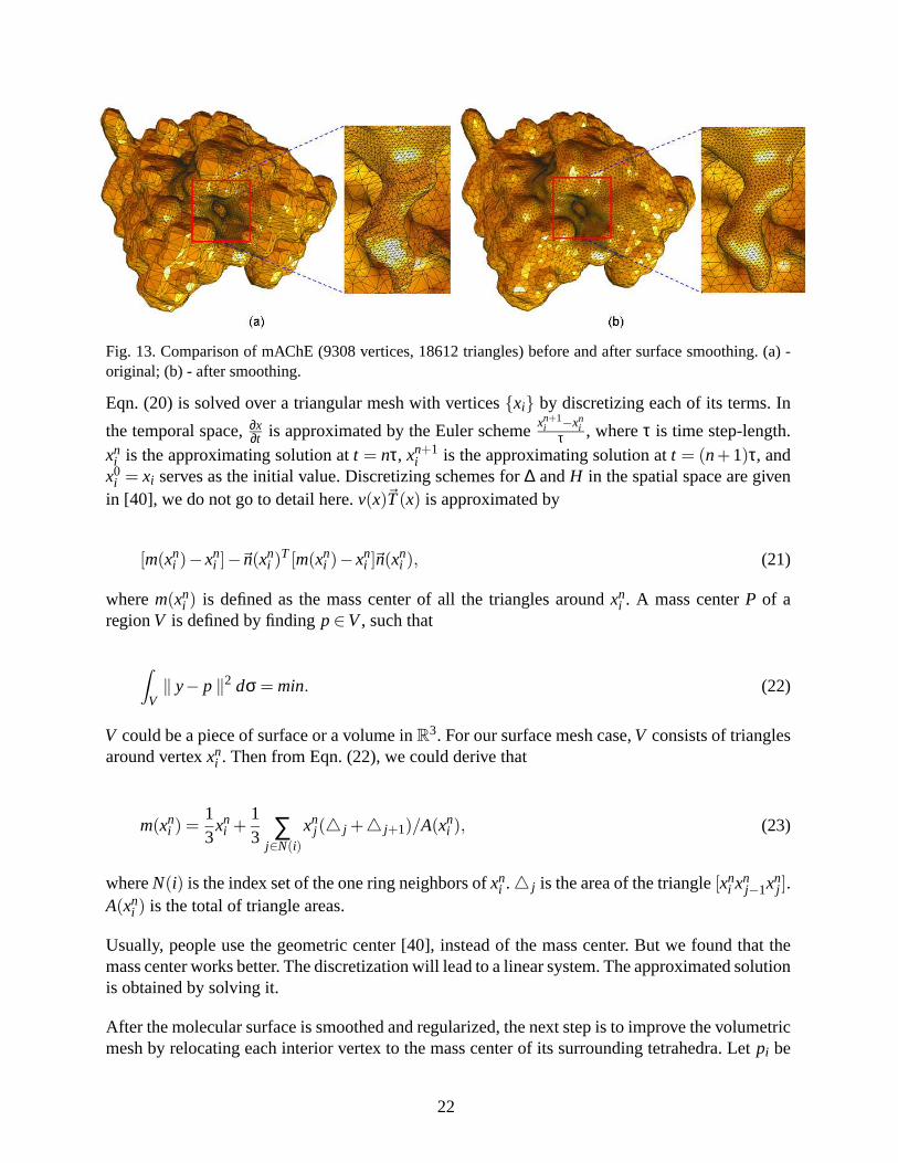
Fig. 13. Comparison of mAChE (9308 vertices, 18612 triangles) before and after surface smoothing. (a) -original; (b) - after smoothing.

Eqn. (20) is solved over a triangular mesh with vertices{xi} by discretizing each of its terms. In

the temporal space,∂x∂t is approximated by the Euler schemexn+1

i −xni

τ , whereτ is time step-length.xn

i is the approximating solution att = nτ, xn+1i is the approximating solution att = (n+1)τ, and

x0i = xi serves as the initial value. Discretizing schemes for∆ andH in the spatial space are given

in [40], we do not go to detail here.v(x)~T(x) is approximated by

[m(xni )−xn

i ]−~n(xni )

T [m(xni )−xn

i ]~n(xni ), (21)

wherem(xni ) is defined as the mass center of all the triangles aroundxn

i . A mass centerP of aregionV is defined by findingp∈V, such that

∫

V‖ y− p ‖2 dσ = min. (22)

V could be a piece of surface or a volume inR3. For our surface mesh case,V consists of triangles

around vertexxni . Then from Eqn. (22), we could derive that

m(xni ) =

13

xni +

13 ∑

j∈N(i)

xnj (△ j +△ j+1)/A(xn

i ), (23)

whereN(i) is the index set of the one ring neighbors ofxni .△ j is the area of the triangle[xn

i xnj−1xn

j ].A(xn

i ) is the total of triangle areas.

Usually, people use the geometric center [40], instead of the mass center. But we found that themass center works better. The discretization will lead to a linear system. The approximated solutionis obtained by solving it.

After the molecular surface is smoothed and regularized, the next step is to improve the volumetricmesh by relocating each interior vertex to the mass center ofits surrounding tetrahedra. Letpi be

22

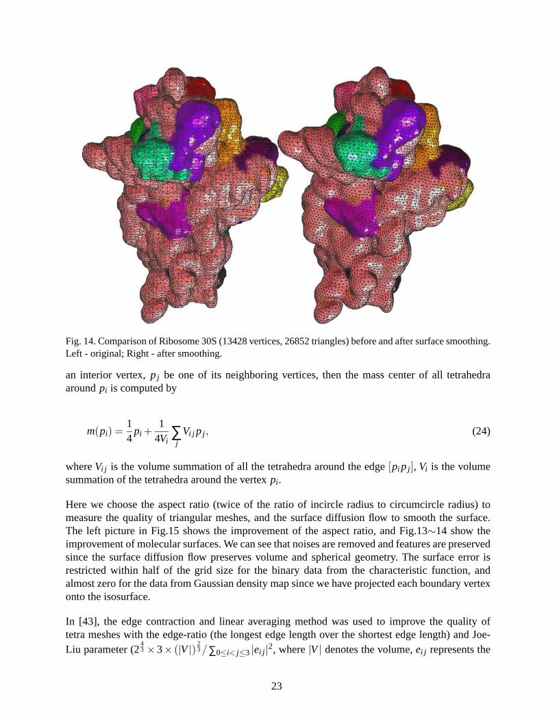
Fig. 14. Comparison of Ribosome 30S (13428 vertices, 26852 triangles) before and after surface smoothing.Left - original; Right - after smoothing.

an interior vertex,p j be one of its neighboring vertices, then the mass center of all tetrahedraaroundpi is computed by

m(pi) =14

pi +1

4Vi∑

jVi j p j , (24)

whereVi j is the volume summation of all the tetrahedra around the edge[pi p j ], Vi is the volumesummation of the tetrahedra around the vertexpi.

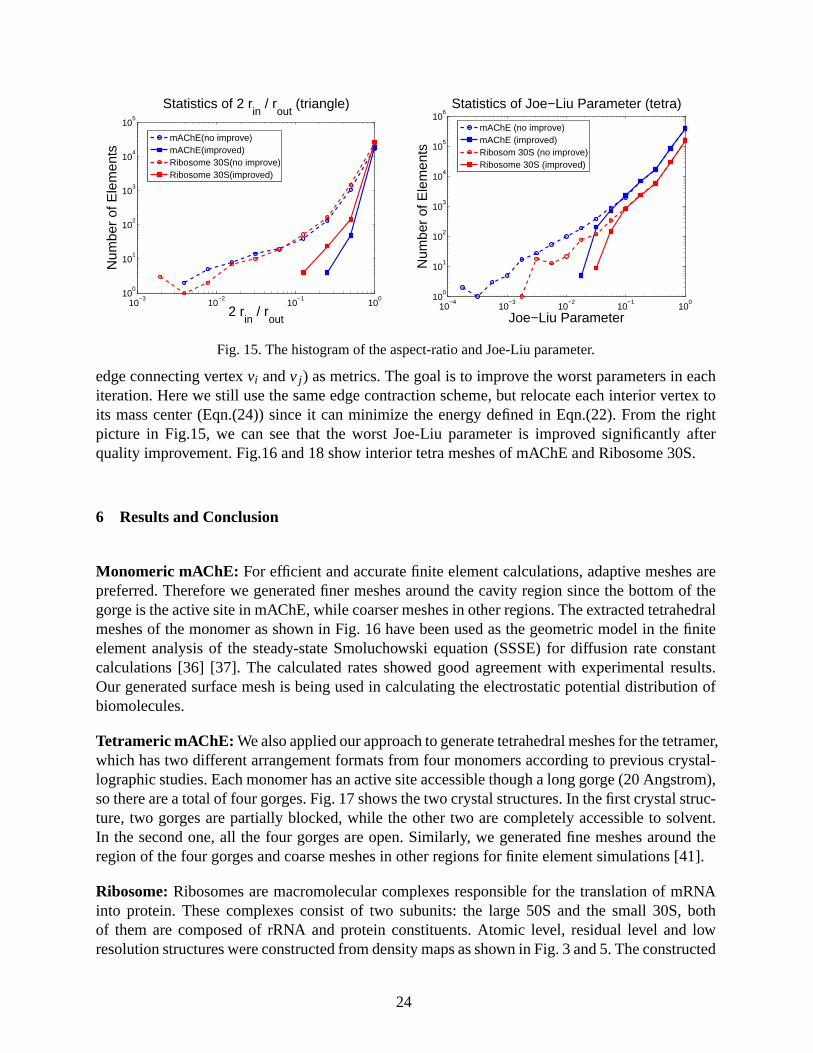
Here we choose the aspect ratio (twice of the ratio of incircle radius to circumcircle radius) tomeasure the quality of triangular meshes, and the surface diffusion flow to smooth the surface.The left picture in Fig.15 shows the improvement of the aspect ratio, and Fig.13∼14 show theimprovement of molecular surfaces. We can see that noises are removed and features are preservedsince the surface diffusion flow preserves volume and spherical geometry. The surface error isrestricted within half of the grid size for the binary data from the characteristic function, andalmost zero for the data from Gaussian density map since we have projected each boundary vertexonto the isosurface.

In [43], the edge contraction and linear averaging method was used to improve the quality oftetra meshes with the edge-ratio (the longest edge length over the shortest edge length) and Joe-Liu parameter (2

43 ×3× (|V|)

23/∑0≤i< j≤3 |ei j |

2, where|V| denotes the volume,ei j represents the

23

10−3

10−2

10−1

100

100

101

102

103

104

105

Statistics of 2 rin

/ rout

(triangle)

2 rin

/ rout

Num

ber

of E

lem

ents

mAChE(no improve)mAChE(improved)Ribosome 30S(no improve)Ribosome 30S(improved)

10−4

10−3

10−2

10−1

100

100

101

102

103

104

105

106

Statistics of Joe−Liu Parameter (tetra)

Joe−Liu Parameter

Num

ber

of E

lem

ents

mAChE (no improve)mAChE (improved)Ribosom 30S (no improve)Ribosome 30S (improved)

Fig. 15. The histogram of the aspect-ratio and Joe-Liu parameter.

edge connecting vertexvi andv j ) as metrics. The goal is to improve the worst parameters in eachiteration. Here we still use the same edge contraction scheme, but relocate each interior vertex toits mass center (Eqn.(24)) since it can minimize the energy defined in Eqn.(22). From the rightpicture in Fig.15, we can see that the worst Joe-Liu parameter is improved significantly afterquality improvement. Fig.16 and 18 show interior tetra meshes of mAChE and Ribosome 30S.

6 Results and Conclusion

Monomeric mAChE: For efficient and accurate finite element calculations, adaptive meshes arepreferred. Therefore we generated finer meshes around the cavity region since the bottom of thegorge is the active site in mAChE, while coarser meshes in other regions. The extracted tetrahedralmeshes of the monomer as shown in Fig. 16 have been used as the geometric model in the finiteelement analysis of the steady-state Smoluchowski equation (SSSE) for diffusion rate constantcalculations [36] [37]. The calculated rates showed good agreement with experimental results.Our generated surface mesh is being used in calculating the electrostatic potential distribution ofbiomolecules.

Tetrameric mAChE: We also applied our approach to generate tetrahedral meshesfor the tetramer,which has two different arrangement formats from four monomers according to previous crystal-lographic studies. Each monomer has an active site accessible though a long gorge (20 Angstrom),so there are a total of four gorges. Fig. 17 shows the two crystal structures. In the first crystal struc-ture, two gorges are partially blocked, while the other two are completely accessible to solvent.In the second one, all the four gorges are open. Similarly, wegenerated fine meshes around theregion of the four gorges and coarse meshes in other regions for finite element simulations [41].

Ribosome: Ribosomes are macromolecular complexes responsible for thetranslation of mRNAinto protein. These complexes consist of two subunits: the large 50S and the small 30S, bothof them are composed of rRNA and protein constituents. Atomiclevel, residual level and lowresolution structures were constructed from density maps as shown in Fig. 3 and 5. The constructed

24

Fig. 16. Interior and exterior tetra meshes of monomeric mAChE. The left two pictures conform to theSAS withσ = 2, and the right two pictures conform to the surface constructed from Gaussian summationwith p1 = 0.25, p2 = 1.0. From left to right: (65147 vertices, 323442 tets), (121670 vertices,656823 tets),(103680 vertices, 509597 tets) and (138967 vertices, 707284 tets). The color shows potential (leftmost) orresidues (the right two).

Fig. 17. Interior and exterior tetra meshes of tetrameric mAChE,p1 = 0.5, p2 = 1.0. The left two picturesshow the 1st crystal structure 1C2O (133078 vertices, 670950 tets), and the right two pictures show the 2ndone 1C2B, (106463 vertices, 551074 tets). Cavities are shown in red boxes.

Fig. 18. Interior and exterior tetra meshes of Ribosome 30S, low resolution,p1 = 0.03125,p2 = 1.0. Fromleft to right: (33612 vertices, 163327 tets), (37613 vertices, 186496 tets) and (40255 vertices, 201724 tets).The pink color shows 16S rRNA and other colors show proteins.

25

various implicit solvation models help to study the machinery of protein production. Fig. 18 andFig. 1 show interior and exterior meshes of Ribosome 30S/50S.

We have developed a quality molecular meshing approach fromPDB data, including implicit sol-vation surface construction from electron density maps, triangular/tetrahedral mesh generation,and quality improvement with surface smoothing. Geometricfeatures are preserved for the molec-ular surface. Some of our generated meshes have been used or is being used in boundary/finiteelement simulations.

Acknowledgments

We wish to thank Vinay Siddavanahalli and John Wiggins for all their help with the generationof smooth volumetric electron density maps using CVC’s fast summation code for biomolecularstructures, and also thank Dr. Yuhua Song, Dr. Deqiang Zhang, Prof. Nathan Baker and Prof.Andrew McCammon for using and helping us calibrate our LBIE mesher for biomolecules. Thework at University of Texas was supported in part by NSF-ITR grants ACI-0220037, EIA-0325550and grants from the NIH 0P20 RR020647 and R01 GM074258. A substantial part of the work onthis paper was done when Prof. Guoliang Xu was visiting Prof.Chandrajit Bajaj at UT-CVC. Hiswork was partially supported by the aforementioned grants,the J.T. Oden ICES fellowship and inpart by Natural Science Foundation of China (10371130) and National Key Basic Research Projectof China (2004CB318000).

References

[1] N. Akkiraju and H. Edelsbrunner. Triangulating the surface of a molecule.Discrete AppliedMathematics, 71:5–22, 1996.

[2] C. Bajaj, J. Castrillon, V. Siddavanahalli, and W. Zhao. Fast calculations of implicit solvationmodels of molecules and solvation energies.Manuscript, 2004.

[3] C. Bajaj, H. Lee, R. Merkert, and V. Pascucci. NURBS based B-rep Models from Macro-molecules and their Properties. InProceedings Fourth Symposium on Solid Modeling andApplications, pages 217–228, 1997.

[4] J. Blinn. A generalization of algebraic surface drawing.ACM Transactions on Graphics,1(3):235–256, 1982.

[5] S. Canann, J. Tristano, and M. Staten. An approach to combined laplacian and optimization-based smoothing for triangular, quadrilateral and quad-dominant meshes. In7th Interna-tional Meshing Roundtable, pages 479–494, 1998.

[6] H.-L. Cheng, T. Dey, H. Edelsbrunner, and J. Sullivan. Dynamic skin triangulation.DiscreteComputational Geometry, 25:525–568, 2001.

[7] S.-W. Cheng, T. Dey, H. Edelsbrunner, M. Facello, and S. Teng. Sliver exudation.ProceedingJournal of ACM, 47:883–904, 2000.

26

[8] P. Chew. Guaranteed-quality delaunay meshing in 3d. InACM Symposium on ComputationalGeometry, pages 391–393, 1997.

[9] H. Edelsbrunner. Deformable smooth surface design.Discrete Computational Geometry,21:87–115, 1999.

[10] D. Field. Laplacian smoothing and delaunay triangulations. Communications in AppliedNumerical Methods, 4:709–712, 1988.

[11] L. Freitag. On combining laplacian and optimization-based mesh smoothing techniqes.AMD-Vol. 220 Trends in Unstructured Mesh Generation, pages 37–43, 1997.

[12] P. Frey, H. Borouchaki, and P.-L. George. Delaunay tetrahedralization using an advancing-front approach. In5th International Meshing Roundtable, pages 31–48, 1996.

[13] I. Fujishiro, Y. Maeda, H. Sato, and Y. Takeshima. Volumetric data exploration using intervalvolume. IEEE Transactions on Visualization and Computer Graphics, 2(2):144–155, 1996.

[14] R.R. Gabdoulline and R.C. Wade. Analytically defined surfaces to analyze molecular inter-action properties.Journal of Molecular Graphics, 14(6):341–353, 1996.

[15] M. Garland and P. Heckbert. Simplifying surfaces with color and texture using quadric errormetrics. InIEEE Visualization, pages 263–270, 1998.

[16] S. Gibson. Using distance maps for accurate surface representation in sampled volumes. InIEEE sympos. on Volume visualization, pages 23–30, 1998.

[17] J. Grant and B. Pickup. A gaussian description of molecular shape.Journal of PhysicalChemistry, 99:3503–3510, 1995.

[18] M. Holst, N. Baker, and F. Wang. Adaptive multilevel finite element solution of the poisson-boltzmann equation i: Algorithms and examples.Journal of Computational Chemistry,21:1319–1342, 2000.

[19] T. Ju, F. Losasso, S. Schaefer, and J. Warren. Dual contouring of hermite data. InSIGGRAPH,pages 339–346, 2002.

[20] L. Kobbelt, M. Botsch, U. Schwanecke, and H. Seidel. Feature sensitive surface extractionfrom volume data. InSIGGRAPH, pages 57–66, 2001.

[21] P. Laug and H. Borouchaki. Molecular surface modeling and meshing. Engineering withComputers, 18:199–210, 2002.

[22] B. Lee and F. Richards. The interpretation of protein structures: Estimation of static accessi-bility. Journal Molecular Biology, 55:379–400, 1971.

[23] M. Lee, M. Feig, F. Salsbury, and C. Brooks. New analytic approximation to standard molec-ular volume definition and its application to generalized born calculation.Journal of Com-putational Chemistry, 24:1348–1356, 2003.

[24] R. Lohner, K. Morgan, and O. Zienkiewicz. Adaptive grid refinement for compressible eulerequations.Accuracy Estimates and Adaptive Refinements in Finite Element Computations,I. Babuska et. al. eds. Wiley, pages 281–297, 1986.

[25] R. Lohner and P. Parikh. Three dimensional grid generation by the advancing-front method.International Journal for Numerical Methods in Fluids, 8:1135–1149, 1988.

[26] W. Lorensen and H. Cline. Marching cubes: A high resolution 3d surface construction algo-rithm. In SIGGRAPH, pages 163–169, 1987.

[27] M. Meyer, M. Desbrun, P. Schr ¨oder, and A. Burr. Discrete differential-geometry operatorsfor triangulated 2-manifolds.VisMath’02, Berlin, 2002.

[28] P. G. Mezey.Shape in Chemistry: An Introduction to Molecular Shape and Topology. VCHPublishers, New York, 1993.

27

[29] G. Nielson and J. Sung. Interval volume tetrahedrization. In IEEE Visualization, pages221–228, 1997.

[30] S. Owen. A survey of unstructured mesh generation technology. In 7th Internat. MeshingRoundtable, pages 26–28, 1998.

[31] M. Sanner, A. Olson, and J. Spehner. Reduced surface: An efficient way to compute molec-ular surfaces.Biopolymers, 38:305–320, 1996.

[32] G. Sapiro. Geometric partial differential equations and imaging analysis.Cambridge Uni-versity Press, 2001.

[33] M. Shephard and M. Georges. Three-dimensional mesh generation by finite octree technique.International Journal for Numerical Methods in Engineering, 32:709–749, 1991.

[34] J. Shewchuk. Constrained delaunay tetrahedrizations and provably good boundary recovery.In 11th International Meshing Roundtable, pages 193–204, 2002.

[35] K. Shimada, A. Yamada, and T. Itoh. Anisotropic triangular meshing of parametric surfacesvia close packing of ellipsoidal bubbles. In6th International Meshing Roundtable, pages375–390, 1997.

[36] Y. Song, Y. Zhang, C. Bajaj, and N. Baker. Continuum diffusion reaction rate calculationsof wild type and mutant mouse acetylcholinesterase: Adaptive finite element analysis.Bio-physical Journal, 87(3):1558–1566, 2004.

[37] Y. Song, Y. Zhang, T. Shen, C. Bajaj, J. McCammon, and N. Baker. Finite element solution ofthe steady-state smoluchowski equation for rate constant calculations.Biophysical Journal,86(4):2017–2029, 2004.

[38] S.-H. Teng and C. Wong. Unstructured mesh generation: Theory, practice and perspectives.International Journal of Computational Geometry and Applications, 10(3):227–266, 2000.

[39] G. Xu. Discrete laplace-beltrami operator on sphere and optimal spherical triangulations.Research Report, Institute of Computational Mathematics and Sciences/Engineering Com-putation, Chinese Academy of Sciences, No. ICM-04-11, 2004.

[40] G. Xu. Discrete laplace-beltrami operators and their convergence.Computer Aided GeometryDesign, 21:767–784, 2004.

[41] D. Zhang, J. Suen, Y. Zhang, Y. Song, Z. Radic, P. Taylor, M. Holst, C. Bajaj, N. Baker,and J. McCammon. Tetrameric mouse acetylcholinesterase: Continuum diffusion rate cal-culations by solving the steady-state smoluchowski equation using finite element methods.Biophysical Journal, 88(3):1659–1665, 2005.

[42] Y. Zhang, C. Bajaj, and B-S Sohn. Adaptive and quality 3d meshing from imaging data. InACM Solid Modeling and Applications, pages 286–291, 2003.

[43] Y. Zhang, C. Bajaj, and B-S Sohn. 3d finite element meshing from imaging data.Specialissue of Computer Methods in Applied Mechanics and Engineering on Unstructured MeshGeneration, in press, 2004.

28