cDNA Microarray Quality Assessment and Quality Control

with BioConductor packages

Nolwenn Le MeurJanuary 2007

Copyright 2007

Outline

Data acquisition & QA/QC Pre-processing Image analysisQuality AssessmentPre-processing and Quality Control

Lab

Scan

(adapted from Duggan et al., Nat. Gen. , 1999)

Two-color Microarray

Test Reference ExcitationLaser 1 Laser 2

Emission

Computer analysisHybridize target

to microarray

Spotting

PCR amplification and purification

RT-PCR

Label withFluor dyes

Oligonucleotides or cDNA clones

Probe (gene reporter)

Cy5 Cy3

Target

Terminology

• Target: DNA hybridized to the array, mobile substrate.

• Probe: DNA spotted on the array (spot).

• print-tip-group :collection of spots printed using the same print-tip (or pin), aka. grid.

• G, Gb: Cy3 signal and background intensities

• R, Rb: Cy5 signal and background intensities

• M = log2(R) - log2(G)

• A = 1/2(log2(R) + log2(G))

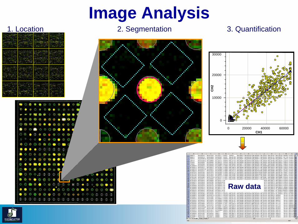
Image Analysis

Intensity (532)0 20000 40000 60000

Inte

nsity

(635

)

0

30000

CH

2

CH1

10000

20000

1. Location 2. Segmentation 3. Quantification

Raw data

Intens ity (532)0 4000 8000

Inte

nsity

(635

)

0

2000

4000

6000

Intens ity (532)0 20000 40000 60000

Inte

nsity

(635

)

0

50000

100000

Intens ity (532)0 2000 4000 6000

Inte

nsity

(635

)

0

1000

2000

Quality Assessment

Intens ity (532)0 20000 40000 60000

Inte

nsity

(635

)

0

10000

20000

30000

• Background• Foreground

Quality AssessmentFor at the probe-level:

Sourcesfaulty printing, uneven distribution, contamination with debris, magnitude of signal relative to noise, poorly measured spots

Spot qualityBrightness: foreground/background ratioUniformity: variation in pixel intensities and ratios of intensities within a spotMorphology: area, perimeter, circularitySpot Size: number of foreground pixels

Actionuse weights for measurements to indicate reliability in later analysis.set measurements to NA (missing values)

Quality AssessmentFor each array

Problemsarray fabrication defectproblem with RNA extractionfailed labeling reactionpoor hybridization conditionsfaulty scanner

Quality measuresPercentage of spots with no signal (~30% exlcuded spots)Range of intensities(Av. Foreground)/(Av. Background) > 3 in both channelsDistribution of spot signal area

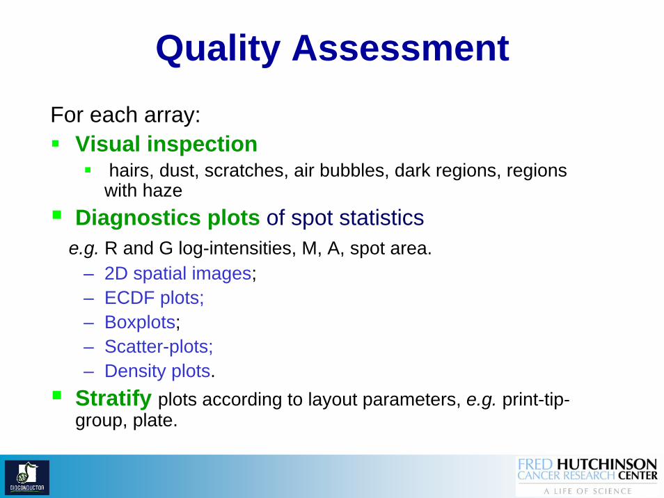
Quality AssessmentFor each array:

Visual inspectionhairs, dust, scratches, air bubbles, dark regions, regions with haze

Diagnostics plots of spot statisticse.g. R and G log-intensities, M, A, spot area.

– 2D spatial images;– ECDF plots;– Boxplots;– Scatter-plots;– Density plots.

Stratify plots according to layout parameters, e.g. print-tip-group, plate.

Image Plots

> library(«marray»)

> data(swirl)

> Gcol <-maPalette(low="white",high="green",k = 50)

> Rcol <-maPalette(low ="white",high="red",k = 50)

>image(swirl[,1],xvar="maRb",col=Rcol)

>image(swirl[,1],xvar="maRf",col=Rcol)

>image(swirl[,1],xvar="maGb",col=Gcol)

>image(swirl[,1],xvar="maRf",col=Gcol)

R R Console

Spatial Effects – Image Plots

R Rb R-Rbcolor scale by rank

Print-tip Washing

Spotting Pin Quality Decline

after delivery of 3x105 spots

after delivery of 5x105 spots

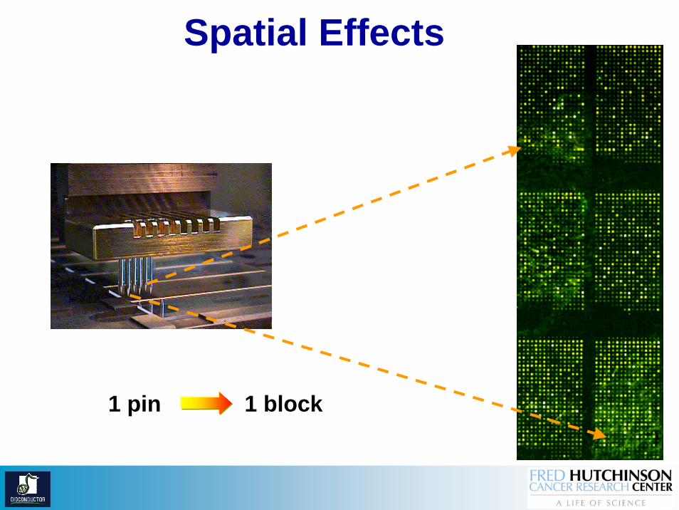
Spatial Effects

1 pin 1 block

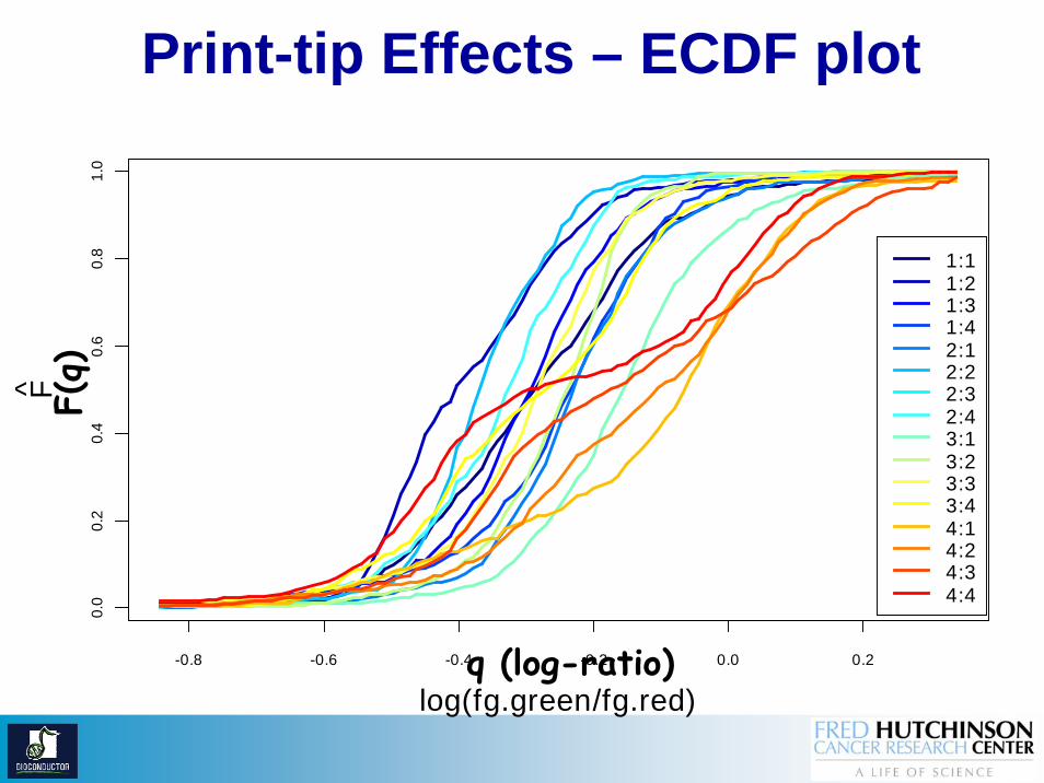
Print-tip Effects – ECDF plot

-0.8 -0.6 -0.4 -0.2 0.0 0.2

0.0

0.2

0.4

0.6

0.8

1.0

41 (a42-u07639vene.txt) by spotting pin

log(fg.green/fg.red)

F̂

1:11:21:31:42:12:22:32:43:13:23:33:44:14:24:34:4

q (log-ratio)

F(q)

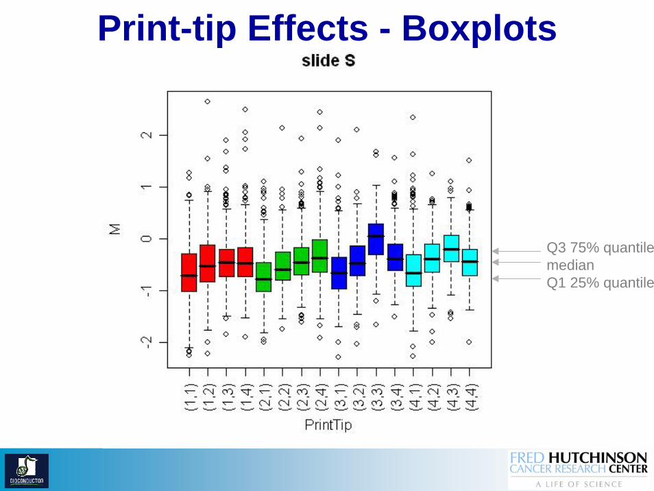
Print-tip Effects - Boxplots

Q3 75% quantilemedianQ1 25% quantile

PCR plates

Diagnostic plot with arrayQuality

library(«arrayQuality»)

?maQualityPlots

R R Console

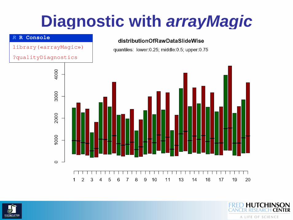
Diagnostic with arrayMagic

library(«arrayMagic»)

?qualityParameters

R R Console

FileName DL32 DL31 DL30 HuPr_4005_DCy3 PEC34_cntrl PEC34_HGF PEC34_SFN+PEC34_SFNCy5 Control Control Control Controlhybridisation HuPr_4008_DL3 HuPr_4007_DL3 HuPr_4006_DHuPr_4005_Dwidth 0.39 0.36 0.43 0.43medianDistance 0.22 0.21 0.25 0.28correlation 0.94 0.95 0.94 0.94correlationLogRaw 0.82 0.86 0.82 0.79meanSignalGreen 2701.65 2664.29 1558.81 2928.64meanSignalRed 2797.52 2683.97 2037.56 3194.82meanSignal 2749.59 2674.13 1798.19 3061.73signalRange.Green 11001.25 11188.90 6289.65 11982.30signalRange.Red 11446.00 11207.00 8602.65 13497.80backgroundRange.Green 21.00 28.00 14.00 23.00backgroundRange.Red 28.00 19.00 28.00 37.00signalToBackground.Green 9.14 8.30 5.67 10.88signalToBackground.Red 14.01 14.00 10.53 16.08

Diagnostic with arrayMagiclibrary(«arrayMagic»)

?qualityDiagnostics

R R Console

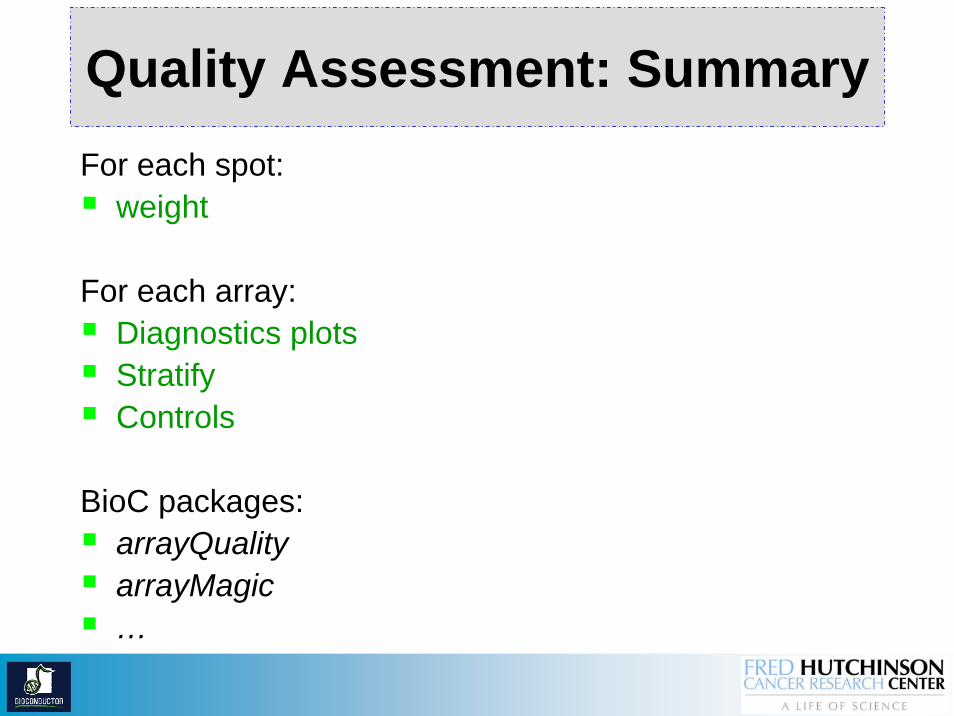
Quality Assessment: SummaryFor each spot:

weight

For each array:Diagnostics plotsStratifyControls

BioC packages:arrayQualityarrayMagic…

Outline

Data acquisition & QA/QC Pre-processing Image analysisQuality AssessmentPre-processing and Quality Control

Lab

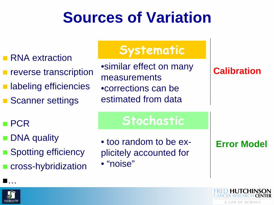
Sources of Variation

PCR DNA quality Spotting efficiencycross-hybridization…

RNA extraction reverse transcription labeling efficienciesScanner settings

Systematic •similar effect on many measurements•corrections can be estimated from data

Stochastic• too random to be ex-plicitely accounted for • “noise”

Calibration

Error Model

Background Correction

none

subtraction, movingmin

Minimun,edwards, normexp,…

More details … limma>?backgroundCorrect

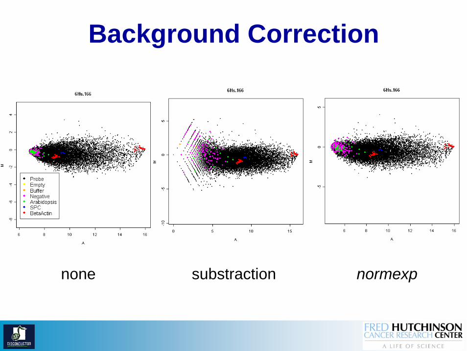
Background Correction

none substraction normexp

Background Correction

NormalizationIdentify and remove the effects of systematic variation

Normalization is closely related to quality assessment. In a ideal experiment, no normalization would be necessary, as the technical variations would have been avoided.

Normalization is needed to ensure that differences in intensities are indeed due to differential expression, and not some printing, hybridization, or scanning artifact.

Normalization is necessary before any analysis which involves between slide comparisons of intensities, e.g., clustering, testing.

Normalization methods

• median• loess • 2D loess• print-tip loess • variance stabilisation• …..

Smyth, G. K., and Speed, T. P. (2003). In: METHODS: Selecting Candidate Genes from DNA Array Screens: Application to Neuroscience

Two-channel

Separate-channel

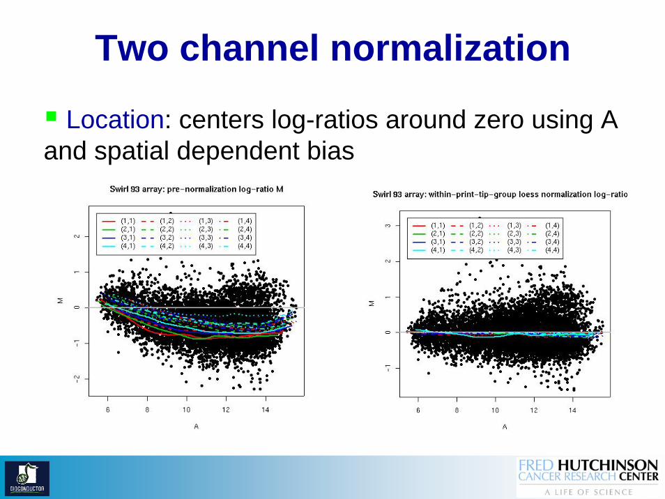
Two channel normalization

Location: centers log-ratios around zero using A and spatial dependent bias

Two channels normalization

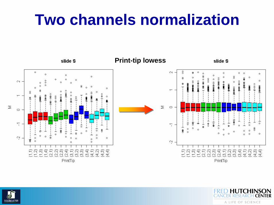
Print-tip lowess

Two channels normalization

Location: centers log-ratios around zero using A and spatial dependent bias

Scale: adjust for different in scale between multiple arrays

median centered median centered & MAD scaled

Scaling

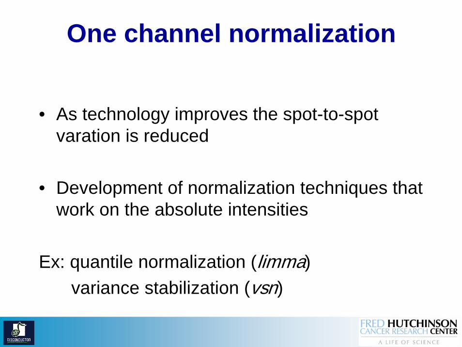
One channel normalization

• As technology improves the spot-to-spot varation is reduced

• Development of normalization techniques that work on the absolute intensities

Ex: quantile normalization (limma)variance stabilization (vsn)

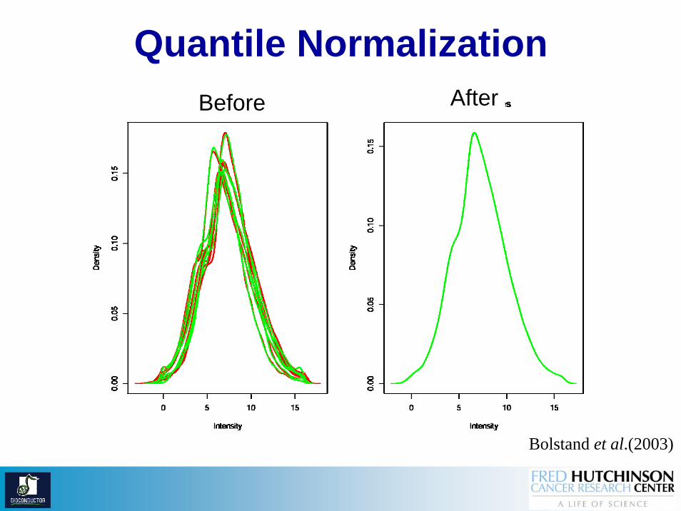
Quantile Normalization

Bolstand et al.(2003)

Before After

Variance StabilizationTransformation

(Huber et al. 2004)intensity

-200 0 200 400 600 800 1000

- - - log

—— arsinh

Estimation of transformation parameters (location, scale) based on Maximun Likelihoodparadigm

vsn–normalized data behaves close to the normal distribution

log-transformation is replaced by a arsinh transformationMeaningful around 0Original intensities may be negatives

Variance Stabilization

Diagnostic plot with arrayMagic

library(«arrayMagic»)

?qualityDiagnostics

R R Console

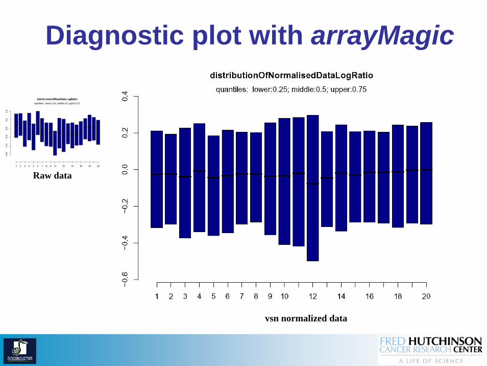
Diagnostic plot with arrayMagic

Raw data

vsn normalized data

Diagnostic plot with arrayMagic

Diagnostic plot with arrayMagic

Preprocessing : Summary

For each array:Background correction or notNormalization Diagnostic plots QA/QC

BioC pacakges:arrayQualityarrayMagicvsnlimma…

BioC Task View: TwoChannel

24 packages (18 Bioc1.8)