Qualitative Robustness in Bayesian Inference

Houman Owhadi and Clint ScovelCalifornia Institute of Technology

December 10, 2014

Abstract

We develop a framework for quantifying the sensitivity of the distribution of pos-terior distributions with respect to perturbations of the prior and data generatingdistributions in the limit when the number of data points grows towards infinity.In this generalization of Hampel [47] and Cuevas’ [18] notion of qualitative robust-ness to Bayesian inference, posterior distributions are analyzed as measure-valuedrandom variables (measures randomized through the data) and their robustness isquantified using the total variation, Prokhorov, and Ky Fan metrics. Our resultsshow that (1) the assumption that the prior has Kullback-Leibler support at theparameter value generating the data, classically used to prove consistency, can alsobe used to prove the non-robustness of posterior distributions with respect to in-finitesimal perturbations (in total variation metric) of the class of priors satisfyingthat assumption, (2) for a prior which has global Kullback-Leibler support on aspace which is not totally bounded, we can establish non qualitative robustness and(3) consistency and robustness are, to some degree, antagonistic requirements anda careful selection of the prior is important if both properties (or their approxima-tions) are to be achieved. The mechanisms supporting our results are different andcomplementary to those discovered by Hampel and developed by Cuevas, and alsoindicate that misspecification generates non qualitative robustness.

Contents

1 Introduction 2

2 Structure of the paper and non-robustness mechanisms 32.1 General set up . . . . . . . . . . . . . . . . . . . . . . . . . . . . . . . . . 32.2 Robustness and Consistency . . . . . . . . . . . . . . . . . . . . . . . . . . 42.3 Mechanisms generating non-robustness . . . . . . . . . . . . . . . . . . . . 6

2.3.1 Robustness under misspecification . . . . . . . . . . . . . . . . . . 92.4 Robustness and Computational Bayesian Inference . . . . . . . . . . . . . 10

3 Lorraine Schwartz’ Theorem 11

1

arX

iv:1

411.

3984

v2 [

mat

h.ST

] 9

Dec

201

4

4 Qualitative Robustness of Bayesian Inference 144.1 Varying the data generating distribution and fixing the prior . . . . . . . 154.2 Varying the prior and fixing the data generating distribution . . . . . . . 154.3 Qualitative Robustness of Bayesian Inference -Definition . . . . . . . . . . 184.4 Proprokhorov Robustness . . . . . . . . . . . . . . . . . . . . . . . . . . . 19

5 Main Results 21

6 Kullback-Leibler Support 24

7 Appendix: Some Prokhorov Geometry 25

8 Proofs 268.1 Proof of Corollary 3.1 . . . . . . . . . . . . . . . . . . . . . . . . . . . . . 268.2 Proof of Proposition 3.4 . . . . . . . . . . . . . . . . . . . . . . . . . . . . 278.3 Proof of Theorem 5.1 . . . . . . . . . . . . . . . . . . . . . . . . . . . . . . 288.4 Proof of Theorem 5.5 . . . . . . . . . . . . . . . . . . . . . . . . . . . . . . 308.5 Proof of Lemma 6.2 . . . . . . . . . . . . . . . . . . . . . . . . . . . . . . 32

Acknowledgments 32

References 32

1 Introduction

Robust Bayesian Analysis [6, 8] seeks to quantify variations in the output of Bayesianinference with respect to perturbations of the model and the prior. The importance ofsuch an effort is expressed by Wasserman, Lavine and Wolpert [89]:

“Most statisticians would acknowledge that an analysis is not complete unlessthe sensitivity of the conclusions to the assumptions is investigated. Yet, inpractice, such sensitivity analyses are rarely used. This is because sensitivityanalyses involve difficult computations that must often be tailored to thespecific problem. This is especially true in Bayesian inference where thecomputations are already quite difficult.”

In the classical Robust Bayesian framework, one defines a model and a prior anddescribes a perturbation class for the model and the prior and then asks, given thespecific value of the data, what is the range of possible conclusions (posterior values)as the model and the prior varies over their perturbation classes. Although robustnesshas been established for classes of finite dimensional perturbations [6, 8, 12, 91], recentresults [71, 70], summarized in [72], suggest that, under finite information, that is,finite codimensional perturbations (e.g., when the class of perturbed priors are definedvia TV/Prokhorov metrics or a finite number of constraints on marginal distributions),Bayesian inference is not only not robust, it is brittle, that is, extremely non-robust.

2

The mechanism generating this brittleness can be seen as an extreme occurrence of thedilation phenomenon [90] which, in robust Bayesian inference, refers to the enlargementof optimal bounds caused by the data dependence of worst priors. This data dependenceof worst priors is inherent to the formulation of classical Bayesian Sensitivity Analysis,in which worst priors are computed given the specific value of the data.

Therefore, although the brittleness results of [71, 70] suggest that Bayesian infer-ence may not be robust under finite information within the classical Robust Bayesianframework [71, 70], one may ask whether robustness could be established under finiteinformation by exiting this strict framework and computing the sensitivity of posteriorconclusions independently of the specific value of the data. To investigate this question,this paper will generalize Hampel [47] and Cuevas’ [18] notion of qualitative robustnessto Bayesian inference based on the quantification of the sensitivity of the distribution ofposterior distributions with respect to perturbations of the prior and the data generatingdistribution, in the limit when the number of data points grows towards infinity. Notethat, contrary to classical Bayesian Sensitivity Analysis, in the proposed formulation,the data is not fixed and posterior values are therefore analyzed as dynamical systemsrandomized through the distribution of the data.

2 Structure of the paper and non-robustness mechanisms

2.1 General set up

We will now describe the general setup allowing us to analyze posterior distributionsas measure-valued random variables or measure-valued dynamical systems randomizedthrough the distribution of the data. We defer measure theoretic technicalities untillater. Let Θ and X be measurable spaces. We write M(X) for the set of probabilitydistributions on X, M(Θ) for the set of probability distributions on Θ and M2(Θ) :=M(M(Θ)

)the set of probability distributions on the set of probability distributions

on Θ. We fix a prior π ∈ M(Θ), a model P : Θ → M(X), and consider a datagenerating distribution µ ∈M(X). Let µn ∈Mn(X) denote the n-fold product measurecorresponding to taking n-i.i.d. samples and for any such n-sample xn from µn, letπxn ∈ M(Θ) denote the posterior measure associated with the prior, model, and thesample. Then we ask how these posteriors πxn vary as a function of the sample data xn

when it is generated by i.i.d. sampling from µ, that is xn ∼ µn. To do so, we considerthe map

π : Xn →M(Θ)

defined by the determination of the posteriors

π(xn) := πxn

and consider its corresponding pushforward operator

π∗ :M(Xn)→M2(Θ) ,

3

where we have removed the bar over π in the notation to remind us that this pushforwardoperator π∗ corresponds to the prior π. Note that π∗µ

n is the sampling distribution ofthe posterior distribution πxn (of the parameter θ) when the data xn is a random variabledistributed according to µn. Since Mn(X) ⊂M(Xn) and µn ∈Mn(X), it follows thatµn ∈M(Xn) so that the pushforward

π∗µn ∈M2(Θ)

is well-defined.In Section 4 we will define the qualitative robustness of Bayesian inference as the

property that π∗µn and π′∗(µ

′)n can be made arbitrarily close for large enough n ifthe priors π and π′ and the data generating distributions µ and µ′ are close enough.In particular, unlike Hampel and Cuevas who require ”for all n” in their definitions,we follow Huber [50] and Mizera [66] in only requiring closeness ”for large enough n”.The results of this paper are applicable to both versions. Most of the non-robustnessmechanisms presented in this paper only require perturbations in the prior distributions(that is, µ = µ′) and so are particularly relevant to well-specified Bayesian inference.Of course the notion of qualitative robustness will depend on the metrics placed on thespace M(X) of data-generating distributions, the space M(Θ) of prior distributions onΘ and the space M2(Θ) of random distributions on Θ. The total variation, Prokhorovand Ky Fan metrics will be of particular interest in our analysis.

2.2 Robustness and Consistency

Since the proposed notion of qualitative robustness is established in the limit when thenumber of data points grows towards infinity, it is natural to expect that the notion ofconsistency (i.e., the property that posterior distributions convergence towards the datagenerating distribution) will play an important role.

Although consistency is primarily a frequentist notion, according to Blackwell andDubins [10] and Diaconis and Freedman [21], consistency is equivalent to intersubjectiveagreement which means that two Bayesians will ultimately have very close predictivedistributions. Therefore, it also has importance for Bayesians. Fortunately, not only arethere mild conditions which guarantee consistency, but the Bernstein-von-Mises theoremgoes further in providing mild conditions under which the posterior is asymptoticallynormal. The most famous of these are Doob [23], Le Cam and Schwartz [62], andSchwartz [80, Thm. 6.1]. For more recent developments, see Barron, Schervish andWasserman [3], Barron [4], Wasserman [88], Ghosh, Ghosal and Ramamoorthi [37],Ghosh [40], Kleijn [58], Walker [86], and the excellent review by Ghosal [36]. Moreover,the assumptions needed for this consistency are so mild that one can be lead to theconclusion that the prior does not really matter once there is enough data. For example,we quote Edwards, Lindeman and Savage [29]:

“Frequently, the data so completely control your posterior opinion that thereis no practical need to attend to the details of your prior opinion.”

4

On the other hand, seemingly paradoxical results regarding inconsistency were foundby Diaconis and Freedman [21, 31], and Freedman [30, 32, 33]: one consequence ofFreedman [33] is that the set of pairs of priors leading to concurring asymptotic posteriorconclusions is meager, i.e. very small in a topological sense.

Moreover, it appears that the full implications of model misspecification, when thedata generating distribution is not exactly in the model class, have only been appreciatedsomewhat recently, see, e.g. Kleijn [57], Grunwald [44], Grunwald and Langford [43],Muller [67], Kleijn and van der Vaart [59, 60], and applied investigations in Biologybegun in Douady et al. [24] and in Economics in Lubik and Schorfheide [63]. We quotefrom Kleijn and van der Vaart [60]:

“In the misspecified situation the posterior distribution of a parameter shrinksto the point within the model at minimum Kullback-Leibler divergence to thetrue distribution, a consistency property that it shares with the maximumlikelihood estimator. Consequently one can consider both the Bayesian pro-cedure and the maximum likelihood estimator as estimates of this minimumKullback- Leibler point. A confidence region for this minimum Kullback-Leibler point can be built around the maximum likelihood estimator basedon its asymptotic normal distribution, involving the sandwich covariance.One might also hope that a Bayesian credible set automatically yields avalid confidence set for the minimum Kullback-Leibler point. However, themisspecified Bernstein-Von Mises theorem shows the latter to be false.”

That is, in the misspecified case, not only do we have inconsistency, we also have strongconvergence -with consequences for confidence sets. Indeed even earlier, to some, theconsistency results appeared to generate more confidence than possibly they should. Wequote A. W. F. Edwards [28, Pg. 60]:

“It is sometimes said, in defence of the Bayesian concept, that the choice ofprior distribution is unimportant in practice, because it hardly influences theposterior distribution at all when there are moderate amounts of data. Theless said about this ’defence’ the better.”

We will demonstrate that the Edwards defence is essentially what produces non qualita-tive robustness in Bayesian inference. In particular, the assumptions required for con-sistency are such that arbitrarily small local perturbations of prior distributions (nearthe data generating distribution) result in consistency or non-consistency, and therefore,have large impacts on the asymptotic behavior of posterior distributions. To make thisprecise, in the following two sections we develop the notions of consistency and robust-ness of Bayesian inference. In particular, in Section 3 we develop the consistency theoremof Schwartz so that it can easily be used in the robustness analysis that is developedSection 4.

A relationship between robustness and consistency has been observed recently inHable and Christmann [46] in ill-posed classification and regression problems, as definedby Dey and Ruymgaart [19], and is based on a fundamental link between robustness and

5

consistency in the results of Hampel [47, Lem. 3] and Cuevas [18, Thm. 1] which can beroughly stated as follows: qualitative robustness and consistency imply that the infinitesample limit is a continuous function of the data generating distribution. Therefore,for consistent systems non qualitative robustness follows from the discontinuity of theinfinite sample limit. This approach has been used by Cuevas [18, Thm. 7] to establishthe non qualitative robustness of two common Bayesian models with fixed priors underperturbations in the data generating distribution.

Moreover, with extra work and stronger but still mild assumptions, rates for consis-tency can be obtained, see e.g. Shen and Wasserman [81], Ghosal, Ghosh, and van derVaart [39], Huang [49], and in the misspecified case Kleijn and van der Vaart [60]. Inparticular, the availability of local conditions guaranteeing rates to consistency has beeninvestigated in Martin, Hong and Walker [65]. We conjecture that when these resultsare applicable, that they can be used to increase the degree of non qualitative robustnessof Bayesian inference in a quantitative way.

Remark 2.1. Cuevas and Hampel use of the word consistency has a different meaningthan the classical one used by, say, Schwartz. That is, to them, consistency denotesthe “convergence” of the distribution of posterior values (in the infinite sample limit)towards a single point. This definition does not require the converge of the distributionof posterior distributions towards the correct point (i.e. the measure corresponding tothe data generating distribution). Therefore, we could paraphrase Hampel and Cuevas’result as Convergence and Robustness implies continuity of the infinite sample limit withrespect to the data generating distribution, whereas Schwartz proves consistency, that isconvergence plus convergence to the correct point. Consequently, weaker theorems suchas those found by Berk [9] in the misspecified case may be sufficient to interact withthe result, or generalizations thereof, of Hampel and Cuevas to generate non qualitativerobustness.

2.3 Mechanisms generating non-robustness

For the clarity of the paper, in this subsection, we introduce some of the mechanismsgenerating non qualitative robustness in Bayesian inference, which complement the mech-anism discovered by Hampel [47, Lem. 3] and Cuevas [18, Thm. 1]. More precisely, thefirst illustrations presented are simplified graphical representations of the mechanismsused to obtain the main (non qualitative robustness) results of Section 5, which do notutilize any misspecification. Then we present mechanisms which appear to generate nonqualitative robustness due to misspecification.

The core mechanism is derived from the nature of both the assumptions and asser-tions of results supporting consistency. A prototypical example of such results, whichwe will use in our proofs, is the corollary to Schwartz’ consistency theorem presented inSection 3. More precisely, using the notations of Section 2.1, Corollary 3.1 states thatif the data generating distribution is µ = P (θ∗) and if the prior π attributes positivemass to every Kullback-Leibler neighborhood of θ∗ ∈ Θ, then the posterior distributionconverges towards δθ∗ as n → ∞. The assumption that π attributes positive mass to

6

Figure 2.1: The data generating distribution is P (θ∗). π′ has most of its mass aroundθ. π is an arbitrarily small perturbation of π′ so that π has Kullback-Leibler support atθ∗. Corollary 3.1 implies that πn converges towards δθ∗ while π′n remains close to δθ.

(a) Density of π (b) Density of π (c) Density of π′

Figure 2.2: The data generating distribution is P (θ∗). The probability density functionsof π and π′ are p and p′ with respect to the uniform distribution on [0, 1]. π is anarbitrarily small perturbation of π′ in total variation. πn converges towards δθ∗ whilethe distance between the support of π′n and θ∗ remains bounded from below by a > 0.

every Kullback-Leibler neighborhood of θ∗ ∈ Θ does not require π to place a significantamount of mass around θ∗, but instead can be satisfied with an arbitrarily small amount.Therefore, if, as in Figure 2.1, π is a prior distribution with support centered aroundθ 6= θ∗, but with a very small amount of mass about θ∗, so that it satisfies the assump-tions of Corollary 3.1 at θ∗, then π can be slightly perturbed into a π′ with support alsocentered around θ 6= θ∗, but with no mass about θ∗. In this situation, although π andπ′ can be made arbitrarily close in total variation distance, the posterior distribution ofπ converges towards δθ∗ as n → ∞, whereas that of π′ remains close to δθ. Figure 2.2gives an illustration of the same phenomenon when the parameter space Θ is the interval[0, 1] and the probability density functions of π and π′ are p and p′ with respect to theuniform measure.

Note that the mechanism illustrated in Figures 2.1 and 2.2 does not generate nonqualitative robustness at all priors but instead for the full class of consistency priors, de-

7

(a) π (b) π′

Figure 2.3: Non-robustness caused by misspecification. The parameter space of themodel is Θ1. We assume that the model P : Θ1 →M(X) is the restriction of an injectivemodel P : Θ1 × Θ2 → M(X) to Θ1 × θ2 = 0. The data generating distribution isP (θ∗) where θ∗ := (θ∗1, θ

∗2), with θ∗2 6= 0, so that the model P is misspecified. π satisfies

Cromwell’s rule. π′ is an arbitrarily small perturbation of π having Kullback-Leiblersupport at θ∗. Corollary 3.1 implies that π′n converges towards δθ∗ while the distancebetween the support of πn and θ∗ remains bounded from below by a > 0.

fined by the assumption of having positive mass on every Kullback-Leibler neighborhoodof θ∗. One may wonder whether this non qualitative robustness can be avoided by select-ing the prior π to satisfy Cromwell’s rule (that is, the assumption that π gives strictlypositive mass to every nontrivial open subset of the parameter space Θ). Theorem 5.4shows that this is not the case if the parameter space Θ is not totally bounded. Forexample, when Θ = R, for all δ > 0 one can find θ ∈ R such that the mass that π placeson the ball of center θ and radius one is smaller than δ, and by displacing this smallamount of mass one obtains a perturbed prior π′ whose posterior distribution remainsasymptotically bounded away from that of π when the data-generating distribution isP (θ). Similarly if Θ is totally bounded then Theorem 5.5 places an upper bound onthe size of the perturbation of the prior π that would be required as a function of thecovering complexity of Θ. Note that these observations suggest that a maximally quali-tatively robust prior should place as much mass as possible near all possible candidates θfor the parameter θ∗ of the data generating distribution, thereby reinforcing the notionthat a maximally robust prior should have its mass spread as uniformly as possible overthe parameter space. We refer to Section 6 for a discussion on the existence of suchmeasures in relation to the geometry of the sets of measures having local and globalKullback-Leibler support.

8

(a) P∗π (b) ν

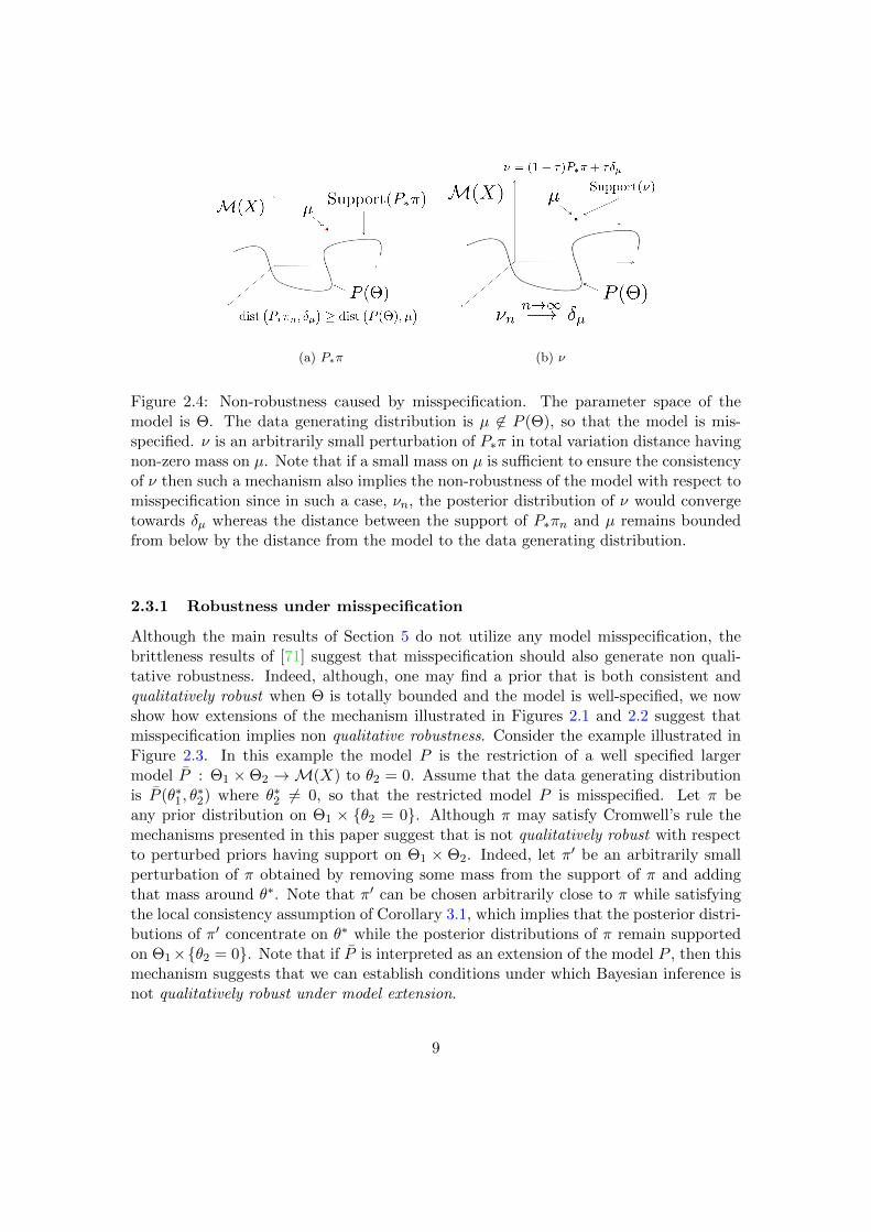
Figure 2.4: Non-robustness caused by misspecification. The parameter space of themodel is Θ. The data generating distribution is µ 6∈ P (Θ), so that the model is mis-specified. ν is an arbitrarily small perturbation of P∗π in total variation distance havingnon-zero mass on µ. Note that if a small mass on µ is sufficient to ensure the consistencyof ν then such a mechanism also implies the non-robustness of the model with respect tomisspecification since in such a case, νn, the posterior distribution of ν would convergetowards δµ whereas the distance between the support of P∗πn and µ remains boundedfrom below by the distance from the model to the data generating distribution.

2.3.1 Robustness under misspecification

Although the main results of Section 5 do not utilize any model misspecification, thebrittleness results of [71] suggest that misspecification should also generate non quali-tative robustness. Indeed, although, one may find a prior that is both consistent andqualitatively robust when Θ is totally bounded and the model is well-specified, we nowshow how extensions of the mechanism illustrated in Figures 2.1 and 2.2 suggest thatmisspecification implies non qualitative robustness. Consider the example illustrated inFigure 2.3. In this example the model P is the restriction of a well specified largermodel P : Θ1 ×Θ2 →M(X) to θ2 = 0. Assume that the data generating distributionis P (θ∗1, θ

∗2) where θ∗2 6= 0, so that the restricted model P is misspecified. Let π be

any prior distribution on Θ1 × θ2 = 0. Although π may satisfy Cromwell’s rule themechanisms presented in this paper suggest that is not qualitatively robust with respectto perturbed priors having support on Θ1 × Θ2. Indeed, let π′ be an arbitrarily smallperturbation of π obtained by removing some mass from the support of π and addingthat mass around θ∗. Note that π′ can be chosen arbitrarily close to π while satisfyingthe local consistency assumption of Corollary 3.1, which implies that the posterior distri-butions of π′ concentrate on θ∗ while the posterior distributions of π remain supportedon Θ1×θ2 = 0. Note that if P is interpreted as an extension of the model P , then thismechanism suggests that we can establish conditions under which Bayesian inference isnot qualitatively robust under model extension.

9

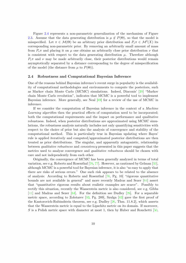
Figure 2.4 represents a non-parametric generalization of the mechanism of Figure2.3. Assume that the data generating distribution is µ 6∈ P (Θ), so that the model ismisspecified. Let π ∈ M(Θ) be an arbitrary prior distribution and P∗π ∈ M2(X) itscorresponding non-parametric prior. By removing an arbitrarily small amount of massfrom P∗π and placing it on µ one obtains an arbitrarily close prior distribution ν thatis consistent with respect to the data generating distribution µ. Therefore althoughP∗π and ν may be made arbitrarily close, their posterior distributions would remainasymptotically separated by a distance corresponding to the degree of misspecificationof the model (the distance from µ to P (Θ)).

2.4 Robustness and Computational Bayesian Inference

One of the reasons behind Bayesian inference’s recent surge in popularity is the availabil-ity of computational methodologies and environments to compute the posteriors, suchas Markov chain Monte Carlo (MCMC) simulations. Indeed, Diaconis’ [20] “Markovchain Monte Carlo revolution”, indicates that MCMC is a powerful tool to implementBayesian inference. More generally, see Neal [69] for a review of the use of MCMC ininference.

If we consider the computation of Bayesian inference in the context of a MachineLearning algorithm then the practical effects of computation need to be incorporated;both the computational requirements and the impact on performance and qualitativerobustness. Indeed, when posterior distributions are approximated using MCMC simu-lations, the robustness analysis naturally includes not only quantifying sensitivities withrespect to the choice of prior but also the analysis of convergence and stability of thecomputational method. This is particularly true in Bayesian updating where Bayes’rule is applied iteratively and computed/approximated posterior distributions are thentreated as prior distributions. The singular, and apparently antagonistic, relationshipbetween qualitative robustness and consistency presented in this paper suggests that themetrics used to analyze convergence and qualitative robustness should be chosen withcare and not independently from each other.

Originally, the convergence of MCMC has been generally analyzed in terms of totalvariation, see e.g. Roberts and Rosenthal [76, 77]. However, as cautioned by Gelman [35],although MCMC is a powerful tool for Bayesian inference, it is also “so easy to apply thatthere are risks of serious errors.” One such risk appears to be related to the absenceof analysis: According to Roberts and Rosenthal [76, Pg. 10] “rigorous quantitativebounds are not available in general” and more recently Madras and Sezer [64] assertthat “quantitative rigorous results about realistic examples are scarce”. Possibly torectify this situation, recently the Wasserstein metric is also considered, see e.g. Gibbs[41] and Madras and Sezer [64]. For the definition see Dudley [26]. For a separablemetric space, according to Zolotarev [93, Pg. 289], Szulga [83] gave the first proof ofthe Kantorovich-Rubinshtein theorem, see e.g. Dudley [26, Thm. 11.8.2], which assertsthat the Wasserstein metric is equal to the Lipschitz metric on its domain. If moreover,S is a Polish metric space with diameter at most 1, then by Huber and Ronchetti [50,

10

Cor. 2.18] we haved2Pr ≤ dW ≤ 2dPr

for all probability measures and, when the diameter is bounded, Gibbs and Su [42,Thm. 2] furthermore show that

d2Pr ≤ dW ≤ (diam(S) + 1)dPr .

Therefore, on Polish metric spaces of bounded diameter, the Wasserstein metric is equiv-alent to the Prokhorov metric and therefore metrizes weak convergence.

Now let us incorporate the MCMC analysis into the robustness analysis when theposteriors are computed using MCMC simulations. Let us further suppose that weare in a situation where we can prove when the computation will have converged, orprove that it has converged using diagnostics such as found in Carlin and Chib [13] andCowles and Carlin [16]. It then appears that incorporating the MCMC simulation intothe robustness analysis makes establishing robustness in any topology stronger than thatwhich we can establish the convergence of the MCMC appear problematic. Consequently,it appears that establishing qualitative robustness of Bayesian inference in the totalvariation topology onM(Θ) might be too much to ask, while weaker topologies, such asthe Wasserstein or Prokhorov topologies, might facilitate practical robustness analysisfor important problems.

3 Lorraine Schwartz’ Theorem

As described in Section 2.2, robustness and consistency are closely related propertiesand consistency will be at the core of the mechanism generating non-robustness. Thebreakthrough in consistency for Bayesian inference is considered to be Schwartz’ theorem[80, Thm. 6.1], so we use it as a model for consistency and the conditions sufficient togenerate it. Stated in Barron, Schervish and Wasserman [3, Intro], Wasserman [88,Pg. 3] and Ghosal, Ghosh and Ramamoorthi [37, Cor. 1] for the nonparametric case, forthe parametric case we will operate in standard Borel spaces; measurable spaces whichare Borel isomorphic with a Borel subset of a Polish metric space. By Schervish [79,Thm. B.32], regular conditional probabilities exist for conditioning random variableswith values in a standard Borel space. Moreover, when the parametric model is aMarkov kernel and is dominated by a σ-finite measure, then by the Bayes’ Theorem fordensities Schervish [79, Thm. 1.31] we have, in addition, that the Bayes’ rule for densitiesdetermines a valid family of densities for the regular conditional distributions. We saythat a model P : Θ→M(X) is dominated if there exists a σ-finite Borel measure ν onX such that Pθ ν, θ ∈ Θ.

Recall the Kullback-Leibler divergence K between two measures µ1 and µ2 definedby

K(µ1, µ2) :=

∫log(dµ1

dν

/dµ2

dν

)dµ1 ,

where ν is any measure such that both µ1 and µ2 are absolutely continuous with respectto ν. It is well known that K is nonnegative, and that it is finite only if µ1 µ2, and

11

in that case K(µ1, µ2) =∫

log dµ1dµ2

dµ1 . From this we can define the Kullback-Leibler

ball Kε(µ) of radius ε about µ ∈ M(X) by Kε(µ) = µ′ ∈ M(X) : K(µ, µ′) ≤ ε.For a model P : Θ → M(X), there is the pullback to a function K on Θ defined byK(θ1, θ2) := K(Pθ1 , Pθ2) and when the model is dominated by a σ-finite measure ν, ifwe let p(x|θ) := dPθ

dν (x), x ∈ X be a realization of the Radon-Nikodym derivative, thenthe pullback has the form

K(θ1, θ2) :=

∫log

p(x|θ1)

p(x|θ2)dPθ1(x) .

From this we define a Kullback-Leibler neighborhood of a point θ ∈ Θ by

Kε(θ) :=θ′ ∈ Θ : K(θ, θ′) ≤ ε

.

Let us define the set of priors K(θ) ⊂ M(Θ) which have Kullback-Leibler support at θby

K(θ) :=π ∈M(Θ) : π

(Kε(θ)

)> 0, ε > 0

,

which implicitly requires that Kε(θ) be measurable1 for all ε > 0. Also let K ⊂ M(Θ)denote those measures with global Kullback-Leibler support, that is,

K := ∩θ∈ΘK(θ)

is the set of priors which have Kullback-Leibler support at all θ, and let Kae ⊃ K, definedby

Kae :=

π ∈M(Θ) : π

θ ∈ Θ : π

(Kε(θ)

)> 0, ε > 0

= 1

, (3.1)

denote the set of priors with almost global Kullback-Leibler support.Let us address the measurability of the Kullback-Leibler neighborhoods Kε(θ) ⊂

Θ, ε > 0. For the nonparametric case, Barron, Schervish and Wasserman [3, Lem. 11]demonstrate that the Kullback-Leibler neighborhoods Kε(Pθ∗) ⊂M(X) are measurablewith respect to the strong topology restricted to the subspace of measures which areabsolutely continuous with respect to a common σ-finite reference measure. For theparametric case, Dupuis and Ellis [27, Lem. 1.4.3] assert that on a Polish space that Kis lower semicontinuous in both arguments. Since the subset embedding : X → X ′ ofa subset X of a metric space X ′ is isometric, when X is a Borel subset of a separablemetric space X ′, it can be shown that the induced pushforward map i∗ : M(X) →M(X ′) is isometric in the Prokhorov metrics, in particular it is continuous. Since thecomposition of a continuous and a lower semicontinuous function is lower semicontinuous,it follows from Dupuis and Ellis [27, Lem. 1.4.3] that on any realization of a standardBorel space that the Kullback-Leibler divergence is lower semicontinuous in each of its

1 Note the change from the standard definition Kε(µ) = µ′ : K(µ, µ′) < ε to ours Kε(µ) = µ′ :K(µ, µ′) ≤ ε does not affect which measures have Kullback-Leibler support, but is more convenientsince then Kε(µ) is closed, simplifying the proof that Kε(θ) is measurable.

12

arguments separately, in particular, fixing the first, it is lower semicontinuous. ThereforeKε(Pθ∗) ⊂ M(X) is closed, and therefore measurable for ε > 0. Consequently, when Pis measurable, it follows that Kε(θ

∗) ⊂ Θ is measurable for ε > 0.The following corollary to Schwartz’ Theorem, and its implications in Proposition

3.4, gives us the form of consistency that we will use in the robustness analysis. Since itassumes the model P : Θ → M(X) is measurable, and since by Aliprantis and Border[1, Thm. 15.13] the map M(X) → R defined by µ 7→ µ(A) is Borel measurable for allA ∈ B(X), it follows that P corresponds to a Markov kernel. Moreover since it alsoassumes the model to be dominated, it follows from Barron, Schervish and Wasserman[3, Lem. 10] that the Radon-Nikodym derivatives can be chosen so that they are B(X)×B(Θ) measurable. Consequently, for a prior π, such a choice determines a well-definedconditional measure πxn for any n-sample xn ∈ Xn. Note the assumption that the mapP : Θ→ P (Θ) be open.

Corollary 3.1 (Schwartz). Let X and Θ be Borel subsets of Polish metric spaces andequip M(X) and M(Θ) with the Prokhorov metric. Consider an injective measurabledominated model P : Θ → M(X) with the family of conditional densities chosen to beB(X) × B(Θ) measurable. Furthermore suppose that P : Θ → P (Θ) is an open map.Then for every π ∈M(Θ) with Kullback-Leibler support at θ∗ ∈ Θ, for every measurableneighborhood U of θ∗, we have

πxn(U)→ 1 n→∞, a.e. P∞θ∗ .

Remark 3.2. Since Θ is a Borel subset of a Polish metric space and P is injective andmeasurable, it follows from Kechris’ [55, Cor. 15.2] corollary to the Lusin-Souslin Theo-rem [55, Thm. 15.1], that P (Θ) ⊂M(X) is Borel. However, the additional assumptionthat P : Θ→ P (Θ) be open is equivalent to assuming that P−1 : P (Θ)→ Θ is continu-ous. In particular, it follows that P−1 : P (Θ)→ Θ is measurable, so that P : Θ→ P (Θ)is a Borel isomorphism.

Remark 3.3. When Θ and X are Borel subsets of Polish metric spaces, if P is injectiveand P (Θ) ⊂ M(X) is discrete, in that every subset of P (Θ) is open in the relativetopology, it follows that P−1 : P (Θ) → Θ is continuous and therefore P : Θ → P (Θ) isopen. In addition, since separable discrete spaces are countable, see e.g. [82, Sec. II.3.8],it follows that P (Θ) is countable and therefore measurable. It also follows that Θ iscountable, although it may not be discrete. Since P−1(A) is countable, and thereforemeasurable, for all measurable A, it follows that P is measurable. Consequently, in thiscase the measurability and openness conditions on the model P of Theorem 5.1 followfrom the assumption that P (Θ) ⊂M(X) be discrete.

It will be useful to express the assertion of Corollary 3.1 and some of its consequencesin terms of the convergence of measures and random measures. To that end, recall thenotation M2(Θ) := M(M(Θ)), and consider the corresponding sequence of randomvariables πn : (X∞, P∞θ∗ ) → M(Θ), defined by πn(x∞) := πxn , x

∞ ∈ X∞, and itsinduced sequence of laws (πn)∗P

∞θ∗ ∈ M2(Θ). Note especially that δδθ∗ is the Dirac

mass in M2(Θ) situated at the Dirac mass δθ∗ in M(Θ) situated at θ∗.

13

Proposition 3.4. The assertion of Corollary 3.1 is equivalent to

πxn 7→ δθ∗ a.e. P∞θ∗ ,

where 7→ is weak convergence. This in turn implies that

P∞θ∗dPr(πn, δθ∗) > ε

→ 0 n→∞ , (3.2)

for ε > 0, which is equivalent to

dPrr

((πn)∗P

∞θ∗ , δδθ∗

)→ 0 n→∞ , (3.3)

where dPrr is the Prokhorov metric on M2(Θ) defined with respect to the Prokhorovmetric dPr on M(Θ).

4 Qualitative Robustness of Bayesian Inference

Hable and Christmann [45] have recently established qualitative robustness for supportvector machines. Hampel [47] introduced the notion of the qualitative robustness ofa sequence of estimators and Cuevas [18] has extended Hampel’s definition and hisbasic structural results to Polish parameter spaces. Boente et al. [11] have developedqualitative robustness for stochastic processes and Nasser et al. [68] for estimation. Theprimary goal of this section is to develop a notion of qualitative robustness for Bayesianinference in the spirit of Hampel. To do so, in Section 4.1, we begin by demonstratinghow Bayesian inference with a fixed prior can naturally be put into Hampel’s framework,following Cuevas [18]. Then, in Section 4.2, we consider fixing the data generatingdistribution, and in Section 4.3 we combine the two into one coherent framework. Finally,in Section 4.4, we define a weaker form based on the Prokhorov metric on the space ofmeasures on the space of measures equipped with the Prokhorov metric, and demonstratehow non-robustness with respect to this weaker form establishes non-robustness for theprimary form. Under the assumptions of Schwartz’ corollary, posterior distributions arewell-defined for any multi-sample, so that for this discussion, we can disregard any well-definedness issues regarding the definition of the posterior and the resulting measuretheoretic technicalities. For the more general case, to incorporate that conditioning isonly defined almost everywhere, we refer to Mizera’s [66] comprehensive extension ofHampel and Cuevas’ results to multivalued mappings.

Of course, there are many variations on this theme, and the choice of metrics willaffect not only the attainability of results, but the relevance of any results obtained.Metrics on spaces of measures is a well studied field, see e.g. Rachev et al. [75] and Gibbsand Su [42], but to keep the presentation simple, here we will restrict our attention tothe total variation, Prokhorov and Ky Fan metrics. On general measurable spaces, wecan metrize the space of measures M(X) and the space of measures on the space ofmeasuresM2(Θ) using total variation. However, when X is metric, we can also metrizethe space of measures M(X) with the Prokhorov metric. In the same way, when Θ is

14

a metric space, we can metrize the space of measures M(Θ) also with the Prokhorovmetric, and having metrized in any way, we can then proceed to metrize M2(Θ) usingthe Prokhorov metric. Moreover, we remind the reader that, unlike Hampel and Cuevaswho require ”for all n” in their definitions, we follow Huber [50] and Mizera [66] in onlyrequiring closeness ”for large enough n”. Finite sample versions, as introduced in Hableand Christmann [46, Def. 2], are also available.

4.1 Varying the data generating distribution and fixing the prior

Following Cuevas [18], we define qualitative robustness when varying the data generatingdistribution and fixing the prior.

Definition 4.1. Let P ⊂ M(X) be an admissible set containing µ ∈ M(X) and letdM(X) and dM2(Θ) be metrics on the spaces M(X) and M2(Θ) respectively. Then wesay that the Bayesian inference for prior π ∈ M(Θ) is qualitatively robust at µ, withrespect to the subset P and the metrics dM(X) and dM2(Θ), if for any ε > 0, there existsa δ > 0 such that

µ ∈ P, dM(X)(µ, µ) < δ =⇒ dM2(Θ)(π∗µn, π∗µ

n) < ε

for large enough n.

Using this setup with Polish spaces and the resulting Prokhorov metrics, Cuevas [18,Thm. 7] proves in two cases, that common Bayesian models with specific fixed priors arenot qualitatively robust.

4.2 Varying the prior and fixing the data generating distribution

Regarding the importance of the robustness of Bayesian inference with respect to theprior, we quote from Berger’s [7] discussion on Diaconis and Ylvisaker [22]:

“There is a very serious issue concerning such an approximation, however,namely the issue of whether this good approximation to the prior ensuresthat the posterior will also be well approximated. I think the answer, ingeneral, is no.”

The stability of Bayesian decision theory with respect to the prior was fully initiatedby Kadane and Chuang [52, 53] and further developed in Chuang [14] and Salinetti [78],and positive results obtained. In particular, in [52] comparison with previous notions,in particular that of Edwards, Lindman and Savage [29], is made. In Kadane andSrinivasan [51, 54] sufficient conditions for the stability of Bayes decision problems underuniform convergence of losses are obtained, generalizing the previously mentioned works[52, 14, 78].

However, we would like to proceed along the lines of Hampel’s approach here, sothat we can combine it with Section 4.1 to obtain a framework for qualitative robustnessfor Bayesian inference which simultaneously includes variation in the prior and the data

15

generating distribution into one Hampel-like framework in a natural way. This has theadded advantage that we can utilize the fundamental results of Hampel [47] and Cuevas[18], and points to further development which will be useful. For example, Mizera [66]has fully developed these notions of qualitative robustness to include both ill-definednessand multi-valuedness, an extension which would be extremely useful for any treatmentof Bayesian inference which incorporates conditioning only being determined almosteverywhere. To that end, let us now develop a definition of qualitative robustness withrespect to variation in the prior, for fixed data generating distribution, based on Hampel.

For a single sample x ∈ X, Basu et al.[5] say that the Bayesian inference is qualita-tively robust at π and x ∈ X, with respect to a metric dM(Θ) onM(Θ) and an admissibleset Π ⊂M(Θ) containing π, if given ε > 0, there exists a δ > 0 such that

π ∈ Π, dM(Θ)(π, π) < δ =⇒ dM(Θ)(πx, πx) < ε

They provide many positive results and some negative results regarding the Prokhorovand Levy metrics. We can extend this definition easily to a sequence x∞ := xi, i = 1, ...,as follows: for the first n, we let xn := xi, i = 1, .., n denote the n-sample and thendefine the sequence of posteriors πxn ∈M(Θ), n = 1, ... Then we say that the Bayesianinference is qualitatively robust at π and x∞ ∈ X∞ using the notion of stability of adynamical system: if, given ε > 0, there exists a δ > 0 such that

π ∈ Π, dM(Θ)(π, π) < δ =⇒ dM(Θ)(πxn , πxn) < ε ,

for large enough n. However, this definition puts no distributional requirements on thesequence x∞. For an i.i.d. sample sequence x∞ ∼ µ∞, we can include the “i.i.d. withrespect to µ” assumption in the definition in a natural way by saying that the Bayesianinference is qualitatively robust at π if given ε1, ε2 > 0, there exists a δ > 0 such that

π ∈ Π, dM(Θ)(π, π) < δ =⇒ µnxn : dM(Θ)(πxn , πxn) > ε1

< ε2

for large enough n. This definition can be calibrated with the following single parameterversion: given ε > 0, there exists a δ > 0 such that

π ∈ Π, dM(Θ)(π, π) < δ =⇒ µnxn : dM(Θ)(πxn , πxn) > ε

< ε (4.1)

for large enough n, where by “calibrated” we mean that if µnxn : dM(Θ)(πxn , πxn) >

ε1< ε2, then if we define ε := max (ε1, ε2), we have

µnxn : dM(Θ)(πxn , πxn) > ε

≤ µn

xn : dM(Θ)(πxn , πxn) > ε1

< ε2

< ε ,

so that we conclude that µnxn : dM(Θ)(πxn , πxn) > ε

< ε, and conversely, if µn

xn :

dM(Θ)(πxn , πxn) > ε< ε, then µn

xn : dM(Θ)(πxn , πxn) > ε1

< ε2 with ε1 := ε, ε2 :=

ε.

16

We now express the condition (4.1) as convergence in probability of M(Θ)-valuedrandom variables and metrize this convergence using the Ky Fan metric. To that end,consider the sequence of maps

πn : X∞ →M(Θ)

defined byπn(x∞) := πxn , x∞ ∈ X∞ .

Then for every µ ∈ M(X), we use the same symbol πn to denote the correspondingsequence

πn : (X∞, µ∞)→M(Θ)

of M(Θ)-valued random variables defined on the probability space (X∞, µ∞).To metrize the condition (4.1) as convergence of the random variables πn using the

Ky Fan metric, recall that for a metric spaces S, the metric d : S×S → R is a continuousfunction and therefore Borel measurable with respect to the Borel σ-algebra B(S × S).However, in general, we have a proper inclusion B(S) × B(S) ⊂ B(S × S), so that, ingeneral, the metric may not be measurable with respect to B(S)×B(S). However, whenS is separable, it follows from Dudley [26, Prop. 4.1.7], that B(S)×B(S) = B(S×S), inwhich case we have the appropriate measurability of the metric function needed in thedefinition of the Ky Fan metric that will follow. This is the reason Rachev et al. [75,Rmk. 2.5.1] restricts attention to separable spaces. See Dudley [25] for the developmentof weak convergence of measures on nonseparable spaces.

For a separable metric space S, probability space (Ω,Σ, P ), and two S-valued randomvariables Z : Ω→ S and W : Ω→ S, the Ky Fan distance between Z and W , see e.g. [26,Pg. 289], is defined as

α(Z,W ) := infε ≥ 0 : P (d(Z,W ) > ε) ≤ ε

. (4.2)

By Dudley [26, Thm. 9.2.2], the Ky Fan metric metrizes convergence in probability ofS-valued random variables from (Ω,Σ, P ).

To proceed, suppose that the metric space(M(Θ), dM(Θ)

)is separable. In partic-

ular, note that when Θ is a separable metric space, such as a Borel subset of a Polishmetric space, then the metric space

(M(Θ), dPr

), where dPr is the Prokhorov metric, is

separable. Then for fixed data generating measure µ and two priors π, π ∈ M(Θ), theidentity

µ∞dM(Θ)

(πn, πn) > ε

= µ∞

x∞ : dM(Θ)

(πn(x∞), πn(x∞)

)> ε

= µnxn : dM(Θ)(πxn , πxn) > ε

implies that the inequality

µnxn : dM(Θ)(πxn , πxn) > ε

< ε

on the righthand side of (4.1) can be written

µ∞dM(Θ)(πn, πn) > ε

< ε

17

which, from the definition (4.2), implies that

αµ(πn, πn) ≤ ε ,

where αµ denotes the Ky Fan metric defined on the space of M(Θ)-valued randomvariables W : (X∞, µ∞)→M(Θ) on the probability space (X∞, µ∞).

Since, for fixed data generating measure µ, the sequence of random variables πn, n =1, .. are all defined on the same probability space (X∞, µ∞), the definition 4.1 of qual-itative robustness now can be stated in terms of the Ky Fan metric on the space ofM(Θ)-valued random variables.

Definition 4.2. Let dM(Θ) be a metric on M(Θ) making it separable. Consider µ ∈M(X), π ∈ M(Θ) and an admissible set Π containing π. Then the Bayesian inferenceis qualitatively robust if given ε > 0, there exists a δ > 0 such that

π ∈ Π, dM(Θ)(π, π) < δ =⇒ αµ(πn, πn) < ε

for large enough n, where αµ is the Ky Fan metric on the space ofM(Θ)-valued randomvariables on the probability space (X∞, µ∞).

This seems to be the most reasonable generalization of Basu et al. [5] to i.i.d se-quences. Of course, other definitions could be used -we simply must specify a metric αµon M(Θ)-valued random variables.

4.3 Qualitative Robustness of Bayesian Inference -Definition

Now we take the ideas of the previous two subsections and combine them to allow thevariation in both the prior and the data generating distribution. Recall from Section 4.1that when the prior π is fixed and we vary the data generating distribution µ, we definea map π : Xn →M(Θ) by

π(xn) := πxn

and use the corresponding pushforward operator

π∗ :M(Xn)→M2(Θ) ,

to pushforward µn toπ∗µ

n ∈M2(Θ) .

Then we say that the Bayesian inference for prior π ∈ M(Θ) is qualitatively robust atµ with respect to an admissible set P containing µ, and metrics dM(X) and dM2(Θ), iffor any ε > 0, there exists a δ > 0 such that

µ ∈ P, dM(X)(µ, µ) < δ =⇒ dM2(Θ)(π∗µn, π∗µ

n) < ε

for large enough n.

18

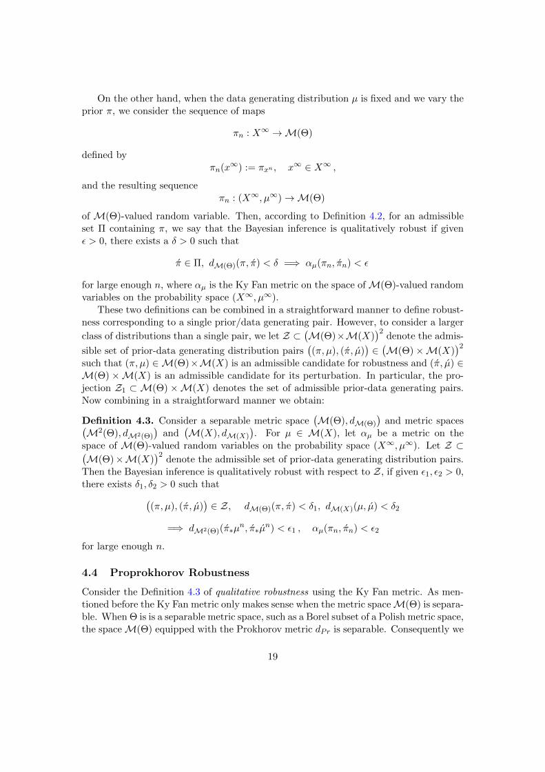
On the other hand, when the data generating distribution µ is fixed and we vary theprior π, we consider the sequence of maps

πn : X∞ →M(Θ)

defined byπn(x∞) := πxn , x∞ ∈ X∞ ,

and the resulting sequenceπn : (X∞, µ∞)→M(Θ)

of M(Θ)-valued random variable. Then, according to Definition 4.2, for an admissibleset Π containing π, we say that the Bayesian inference is qualitatively robust if givenε > 0, there exists a δ > 0 such that

π ∈ Π, dM(Θ)(π, π) < δ =⇒ αµ(πn, πn) < ε

for large enough n, where αµ is the Ky Fan metric on the space ofM(Θ)-valued randomvariables on the probability space (X∞, µ∞).

These two definitions can be combined in a straightforward manner to define robust-ness corresponding to a single prior/data generating pair. However, to consider a larger

class of distributions than a single pair, we let Z ⊂(M(Θ)×M(X)

)2denote the admis-

sible set of prior-data generating distribution pairs((π, µ), (π, µ)

)∈(M(Θ)×M(X)

)2such that (π, µ) ∈M(Θ)×M(X) is an admissible candidate for robustness and (π, µ) ∈M(Θ) ×M(X) is an admissible candidate for its perturbation. In particular, the pro-jection Z1 ⊂ M(Θ) ×M(X) denotes the set of admissible prior-data generating pairs.Now combining in a straightforward manner we obtain:

Definition 4.3. Consider a separable metric space(M(Θ), dM(Θ)

)and metric spaces(

M2(Θ), dM2(Θ)

)and

(M(X), dM(X)

). For µ ∈ M(X), let αµ be a metric on the

space of M(Θ)-valued random variables on the probability space (X∞, µ∞). Let Z ⊂(M(Θ)×M(X)

)2denote the admissible set of prior-data generating distribution pairs.

Then the Bayesian inference is qualitatively robust with respect to Z, if given ε1, ε2 > 0,there exists δ1, δ2 > 0 such that(

(π, µ), (π, µ))∈ Z, dM(Θ)(π, π) < δ1, dM(X)(µ, µ) < δ2

=⇒ dM2(Θ)(π∗µn, π∗µ

n) < ε1 , αµ(πn, πn) < ε2

for large enough n.

4.4 Proprokhorov Robustness

Consider the Definition 4.3 of qualitative robustness using the Ky Fan metric. As men-tioned before the Ky Fan metric only makes sense when the metric spaceM(Θ) is separa-ble. When Θ is is a separable metric space, such as a Borel subset of a Polish metric space,the spaceM(Θ) equipped with the Prokhorov metric dPr is separable. Consequently we

19

now fix it to be (M(Θ), dPr). Let us call Definition 4.3 using the Ky Fan metric definedon the space of (M(Θ), dPr)-valued random variables Ky Fan-Prokhorov robustness. Wenow define a weaker notion of qualitative robustness which we call Proprokhorov robust-ness such that Ky Fan-Prokhorov robustness implies Proprokhorov robustness. Conse-quently, and most importantly, Proprokhorov non-robustness implies Ky Fan-Prokhorovnon-robustness. This weaker robustness has two distinct advantages. The first is thatit has a simpler expression than Ky Fan-Prokhorov robustness and the second is thatit is simpler to analyze. This simpler structure amounts to the Prokhorov metric onthe space of probability measures on the space of probability measures equipped withthe Prokhorov metric, suggesting the name Prokhorov-Prokhorov robustness, which wehave shortened to Proprokhorov. Basic results which we will need regarding this metricspace are derived in the appendix, Section 7.

To proceed, for fixed π and µ, the sequence

πn : (X∞, µ∞)→M(Θ) , n = 1, ...

of M(Θ)-valued random variables can be used to pushforward µ∞ to the sequence

(πn)∗µ∞ ∈M2(Θ) , n = 1, ...

of laws in M2(Θ). Since, by definition πn(x∞) := πxn and the maps π : Xn → M(Θ)were defined by π(xn) := πxn , dropping the ¯ in the notation, it follows that

π∗µn = (πn)∗µ

∞, n = 1, ... (4.3)

According to Dudley [26, Thm. 11.3.5], for S-valued random variables Z,W from thesame probability space, with laws µZ , µW , we have

dPr(µZ , µW ) ≤ α(Z,W ) . (4.4)

Let us denote the Prokhorov metric on the spaceM2(Θ) by dPrr. Then for fixed µ andpriors π and π, it follows from (4.3) and the Prokhorov-Ky Fan inequality (4.4) that

dPrr(π∗µn, π∗µ

n) = dPrr((πn)∗µ

∞, (πn)∗µ∞)

≤ αµ(πn, πn)

and so we conclude that

dPrr(π∗µn, π∗µ

n) ≤ αµ(πn, πn) , n = 1, ... .

From the triangle inequality we then obtain

dPrr(π∗µn, π∗µ

n) ≤ dPrr(π∗µn, π∗µ

n) + dPrr(π∗µn, π∗µ

n)

≤ αµ(πn, πn) + dPrr(π∗µn, π∗µ

n) ,

bounding the simple single term dPrr(π∗µn, π∗µ

n) in terms of the two terms αµ(πn, πn)and dPrr(π∗µ

n, π∗µn) of Ky Fan-Prokhorov robustness, defined in 4.3 using the Pro-

prokhorov metric dPrr on M2(Θ). Using the term dPrr(π∗µn, π∗µ

n) to define Pro-prokhorov robustness, it therefore follows that Ky Fan-Prokhorov robustness implies

20

Proprokhorov robustness articulated with respect to three parameters δ1, δ2 and ε andthe Proprokhorov metric. By putting a metric on M(Θ) ×M(X) which is consistentwith the product metric, we state an equivalent version in terms of two parameters δand ε.

Definition 4.4 (Proprokhorov Robustness). Let(M(X), dM(X)

)be a metric space and

let Θ be a separable metric space and consider the separable metric spaces(M(Θ), dPr)

and(M2(Θ), dPrr

). Let d be a metric which is consistent with the product metric

dPr × dM(X) onM(Θ)×M(X) . Let Z ⊂(M(Θ)×M(X)

)2denote the admissible set

of prior-data generating distribution pairs. Then the Bayesian inference is qualitativelyrobust with respect to Z, if given ε > 0, there exists a δ > 0 such that(

(π, µ), (π, µ))∈ Z, d

((π, µ), (π, µ)

)< δ, =⇒ dPrr(π∗µ

n, π∗µn) < ε

for large enough n.

Since it is essential for our main results, we summarize the fact that Proprokhorovrobustness is weaker than Ky Fan-Prokhorov robustness.

Theorem 4.5. Let(M(X), dM(X)

)be a metric space and let Θ be a separable metric

space. Then Ky Fan-Prokhorov robustness of Definition 4.3, using the Ky Fan metricon the space of (M(Θ), dPr)-valued random variables, implies Proprokhorov robustnessof Definition 4.4.

5 Main Results

Now that we have defined qualitative robustness for Bayesian inference and presentedthe consistency conditions of Section 3, we are now prepared for our main results. In-deed, the brittleness results of [71, 70, 72] and the non qualitative robustness results ofCuevas [18, Thm. 7] suggest that we may obtain non qualitative robustness according toDefinition 4.3 by fixing the prior and varying the data generating distribution. However,according to Berk [9], in the misspecified case, although ”there need be no convergence(in any sense)”, in the limit the posterior becomes confined to a carrier set consistingof those points which are closest in terms of the Kullback-Leibler divergence. Conse-quently, it appears possible that a generalization of the results of Hampel [47, Lem. 3]and Cuevas [18, Thm. 1] which allows such a set-valued notion of consistency may besufficient. Certainly it will require the more sophisticated notions of the continuity, orsemi-continuity, of the Kullback-Leibler set-valued information projection and its de-pendence on the geometry of the model class P (Θ) ⊂ M(X). Although this path willcertainly be instructive and appears feasible, we instead find it simpler to obtain nonqualitative robustness by fixing the data generating distribution to be in the model classand varying the prior. In particular, we show that the inference is not Proprokhorovrobust according to Definition 4.4. It then follows from Theorem 4.5 that it is not KyFan-Prokhorov robust according to Definition 4.3, when the Ky Fan metric is definedon (M(Θ), dPr)-valued random variables. It is important to note that these results do

21

not require any misspecification. Moreover, it appears that Bayesian Inference’s depen-dence on both the data generating distribution and the prior leads to two complementarymechanisms generating non qualitative robustness; whereas Cuevas’ result [18, Thm. 7]utilizes consistency and the discontinuity of the infinite sample limit, this other compo-nent utilizes the non-robustness of consistency, namely that the set of consistency priors,those with Kullback-Leibler support at the data generating distribution, is not robust.

Now let us return to our main results. For θ ∈ Θ, let us denote the set of priors withKullback-Leibler support at θ by

K(θ) := π ∈M(Θ) : π has Kullback-Leibler support at θ

and, for ρ > 0, define a total variation uniformity Πρ(θ) ⊂M(Θ)×M(Θ) by

Πρ(θ) := (π, π) ∈M(Θ)×M(Θ) : π ∈ K(θ), dtv(π, π) < ρ

of prior pairs where the first component has Kullback-Leibler support at θ and the secondcomponent is within ρ of the first in the total variation metric. For θ ∈ Θ, we define anadmissible set of prior-data generating distribution pairs Zρ(θ) ⊂

(M(Θ)×M(X)

)2by

Zρ(θ) := Πρ(θ)× Pθ × Pθ , (5.1)

using the identification of(M(Θ)×M(X)

)2with M(Θ)×M(Θ)×M(X)×M(X).

Our Main Theorem shows, under the conditions of Schwartz’ Corollary, that theBayesian inference is not robust under the assumption that the prior has Kullback-Leibler support at the parameter value generating the data.

Theorem 5.1. For all θ ∈ Θ, given the conditions of Schwartz’ Corollary 3.1, theBayesian inference is not Proprokhorov robust at Zρ(θ) for all ρ > 0.

Remark 5.2. Actually the proof shows more; let D denote the diameter of Θ, then forε < min (D2 , 1), there does not exist a δ > 0 such that the Definition 4.4 of Proprokhorovrobustness is satisfied. Since min (D2 , 1) is large, either half the diameter of the space orlarger than 1, we say the inference is brittle.

Remark 5.3. In particular, Theorem 4.5 implies that the inference is not Ky Fan-Prokhorov robust.

Theorem 5.1 does not assert that the Bayesian inference is not robust at any specifiedprior, only that it is not robust under the assumption that the prior has Kullback-Leiblersupport at the parameter value generating the data. To establish non-robustness atspecific priors we include variation in the data-generating distribution in the model classas follows. Let ∆P ⊂M(X)×M(X), defined by

∆P = (Pθ, Pθ), θ ∈ Θ ,

denote the fact that we allow the data generating distribution to vary throughout themodel class but do not allow any perturbations to it. Then, for π ∈ M(Θ), define the

admissible set Zρ(π) ⊂(M(Θ)×M(X)

)2by

Zρ(π) := π ×Btvρ (π)×∆P ,

22

where Btvρ (π) is the open ball in the total variation metric.

Since the following theorem is a corollary to the theorem after it, Theorem 5.5, wedo not include its proof. However, we state it here because it is the more fundamentalresult.

Theorem 5.4. Given the conditions of Schwartz’ Corollary 3.1 with Θ not totallybounded. Then if the prior π has Kullback-Leibler support for all θ ∈ Θ, the Bayesianinference is not Proprokhorov robust at Zρ(π) for all ρ > 0.

Since a metric space is totally bounded if and only if its completion is compact,when Θ is totally bounded, we assume that it is a Borel subset of a compact metricspace. In this case, although Theorem 5.4 does not apply, utilizing the covering numberand packing number inequalities of Kolmogorov and Tikhomirov [61], we can providea natural quantification of qualitative robustness. To that end, we define covering andpacking numbers. For a finite subset Θ′ ⊂ Θ, the finite collection of open balls Bε(θ), θ ∈Θ′ is said to constitute a covering of Θ if Θ ⊂ ∪θ∈Θ′Bε(θ). For a finite set Θ′ we denoteits size by |Θ′|. The covering numbers are defined by

Nε(Θ) = min|Θ′| : Θ ⊂ ∪θ∈Θ′Bε(θ)

,

that is, Nε(Θ) is the smallest number of open balls of radius ε centered on points inΘ which covers Θ. On the other hand, a set of points Θ′ ⊂ Θ is said to constitute anε-packing if d(θ1, θ2) ≥ ε, θ1 6= θ2 ∈ Θ′. The packing numbers are then defined by

Mε(Θ) := max|Θ′| : Θ′ is an ε-packing of Θ

.

Since the Kolmogorov and Tikhomirov [61, Thm. IV] inequalities

M2ε(Θ) ≤ Nε(Θ) ≤Mε(Θ) (5.2)

are valid in the not totally bounded case, if we allow values of ∞, the following theoremhas Theorem 5.4 as its corollary.

Theorem 5.5. Given the conditions of Theorem 5.4 with Θ totally bounded and ρ > 0.If the Bayesian inference is Proprokhorov robust, then given ε > 0, in terms of theproduct metric we must have

δ < min( 1

N2ε(Θ), ρ).

Remark 5.6. Although the total variation metric on M(Θ) is not used in the metricdefining qualitative robustness for separability, measurability, and consistency purposes,the definition of the admissible sets Zρ(θ) and Zρ(π) in terms of the total variationmetric and a look at the proofs, can be used to show that these non qualitative robustnessresults primarily depend on total variation and do not arise because of the use of theweak topology.

23

6 Kullback-Leibler Support

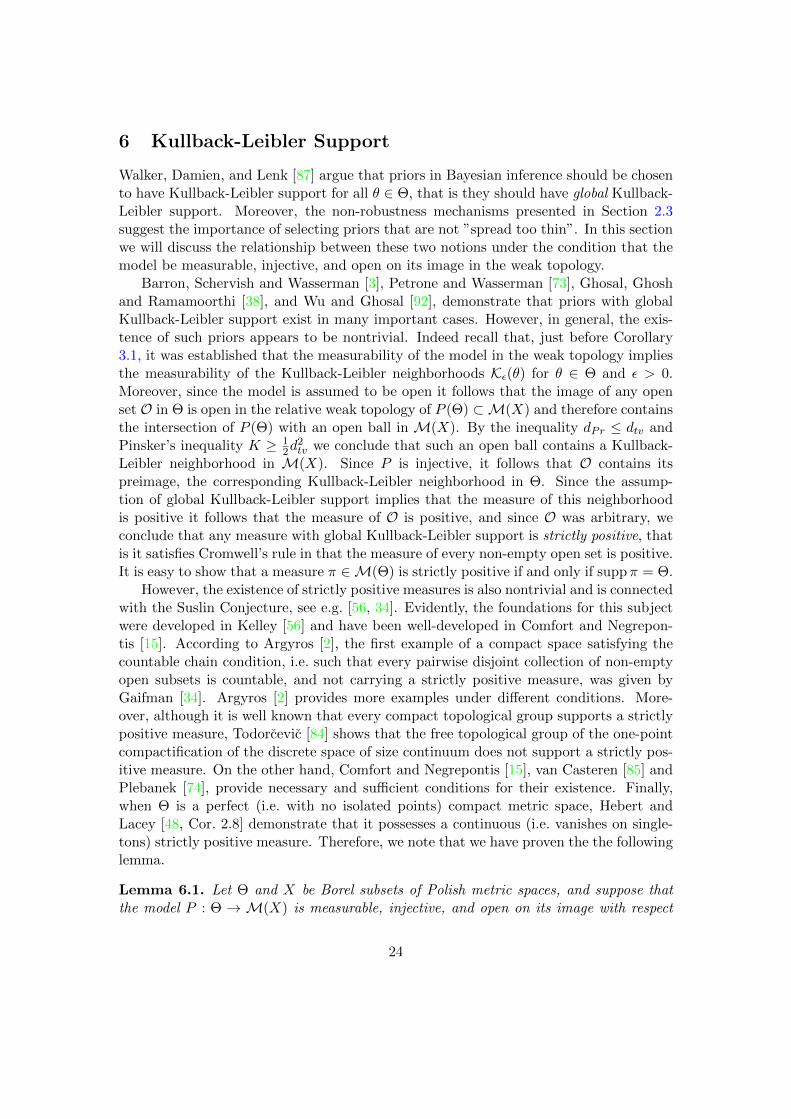
Walker, Damien, and Lenk [87] argue that priors in Bayesian inference should be chosento have Kullback-Leibler support for all θ ∈ Θ, that is they should have global Kullback-Leibler support. Moreover, the non-robustness mechanisms presented in Section 2.3suggest the importance of selecting priors that are not ”spread too thin”. In this sectionwe will discuss the relationship between these two notions under the condition that themodel be measurable, injective, and open on its image in the weak topology.

Barron, Schervish and Wasserman [3], Petrone and Wasserman [73], Ghosal, Ghoshand Ramamoorthi [38], and Wu and Ghosal [92], demonstrate that priors with globalKullback-Leibler support exist in many important cases. However, in general, the exis-tence of such priors appears to be nontrivial. Indeed recall that, just before Corollary3.1, it was established that the measurability of the model in the weak topology impliesthe measurability of the Kullback-Leibler neighborhoods Kε(θ) for θ ∈ Θ and ε > 0.Moreover, since the model is assumed to be open it follows that the image of any openset O in Θ is open in the relative weak topology of P (Θ) ⊂M(X) and therefore containsthe intersection of P (Θ) with an open ball in M(X). By the inequality dPr ≤ dtv andPinsker’s inequality K ≥ 1

2d2tv we conclude that such an open ball contains a Kullback-

Leibler neighborhood in M(X). Since P is injective, it follows that O contains itspreimage, the corresponding Kullback-Leibler neighborhood in Θ. Since the assump-tion of global Kullback-Leibler support implies that the measure of this neighborhoodis positive it follows that the measure of O is positive, and since O was arbitrary, weconclude that any measure with global Kullback-Leibler support is strictly positive, thatis it satisfies Cromwell’s rule in that the measure of every non-empty open set is positive.It is easy to show that a measure π ∈M(Θ) is strictly positive if and only if suppπ = Θ.

However, the existence of strictly positive measures is also nontrivial and is connectedwith the Suslin Conjecture, see e.g. [56, 34]. Evidently, the foundations for this subjectwere developed in Kelley [56] and have been well-developed in Comfort and Negrepon-tis [15]. According to Argyros [2], the first example of a compact space satisfying thecountable chain condition, i.e. such that every pairwise disjoint collection of non-emptyopen subsets is countable, and not carrying a strictly positive measure, was given byGaifman [34]. Argyros [2] provides more examples under different conditions. More-over, although it is well known that every compact topological group supports a strictlypositive measure, Todorcevic [84] shows that the free topological group of the one-pointcompactification of the discrete space of size continuum does not support a strictly pos-itive measure. On the other hand, Comfort and Negrepontis [15], van Casteren [85] andPlebanek [74], provide necessary and sufficient conditions for their existence. Finally,when Θ is a perfect (i.e. with no isolated points) compact metric space, Hebert andLacey [48, Cor. 2.8] demonstrate that it possesses a continuous (i.e. vanishes on single-tons) strictly positive measure. Therefore, we note that we have proven the the followinglemma.

Lemma 6.1. Let Θ and X be Borel subsets of Polish metric spaces, and suppose thatthe model P : Θ → M(X) is measurable, injective, and open on its image with respect

24

to the weak topology. If Θ does not possess a strictly positive probability measure, thenK = ∅.

In the situation of Lemma 6.1, although Theorem 5.4 does not apply, an almosteverywhere version of it can be proved under the the weaker assumption that π hasalmost global Kullback-Leibler support, that is π ∈ Kae as defined in (3.1).

The following result illustrates density properties of the sets of measures with Kullback-Leibler support.

Lemma 6.2. Let Θ and X be Borel subsets of Polish metric spaces and consider ameasurable model P : Θ→M(X), where M(X) is equipped with weak topology, and theresulting Kullback-Leibler divergence K on Θ×Θ. Then the set of probability measuresK(θ) with Kullback-Leibler support at θ is a convex dense subset of M(Θ) in the totalvariation topology. Moreover, if the set of probability measures K := ∩θ∈ΘK(θ) withKullback-Leibler support at all θ ∈ Θ is non-empty, it is a convex dense subset.

7 Appendix: Some Prokhorov Geometry

We establish a basic mechanism to bound from below the Prokhorov distance betweentwo measures based on the values of the measures on the neighborhood of a single set.

Lemma 7.1. Let Z be a metric space and consider the space M(Z) of Borel probabilitymeasures equipped with the Prokhorov metric. Consider µ ∈ M(Z) and suppose thatthere exists a set B ∈ B(Z) and α, δ ≥ 0 such that

µ(Bε) ≤ δ, ε < α .

Then, for any µ′ ∈M(Z), we have

dPr(µ, µ′) ≥ min

(α, µ′(B)− δ

).

Proof. If dPr(µ1, µ2) ≥ α the assertion is proved, so let us assume that dPr(µ1, µ2) < α.Then, denoting d∗ := dPr(µ1, µ2), it follows from the assumption that µ(Ad

∗) ≤ δ, so

that

µ′(A) ≤ µ(Ad∗) + d∗

≤ δ + d∗

from which we conclude that µ′(A) − δ ≤ d∗. Therefore, either dPr(µ1, µ2) ≥ α ordPr(µ1, µ2) ≥ µ′(A)− δ, proving the assertion.

Lemma 7.2. Let S be a separable metric space. Then, for an S-valued random variableX we have

α(X, s) = dPr(L(X), δs)

where α is the Ky Fan metric and s denotes the random variable with constant value s.

25

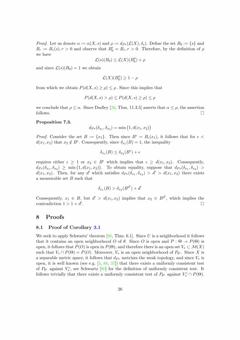
Proof. Let us denote α := α(X, s) and ρ := dPr(L(X), δs). Define the set B0 := s andBr := Br(s), r > 0 and observe that Br

0 = Br, r > 0. Therefore, by the definition of ρwe have

L(s)(B0) ≤ L(X)(Bρ0) + ρ

and since L(s)(B0) = 1 we obtain

L(X)(Bρ0) ≥ 1− ρ

from which we obtain P (d(X, s) ≥ ρ) ≤ ρ . Since this implies that

P (d(X, s) > ρ) ≤ P (d(X, s) ≥ ρ) ≤ ρ

we conclude that ρ ≤ α. Since Dudley [26, Thm. 11.3.5] asserts that α ≤ ρ, the assertionfollows.

Proposition 7.3.dPr(δx1 , δx2) = min

(1, d(x1, x2)

)Proof. Consider the set B := x1. Then since Bε = Bε(x1), it follows that for ε <d(x1, x2) that x2 /∈ Bε. Consequently, since δx1(B) = 1, the inequality

δx1(B) ≤ δx2(Bε) + ε

requires either ε ≥ 1 or x2 ∈ Bε which implies that ε ≥ d(x1, x2). Consequently,dPr(δx1 , δx2) ≥ min

(1, d(x1, x2)

). To obtain equality, suppose that dPr(δx1 , δx2) >

d(x1, x2). Then, for any d′ which satisfies dPr(δx1 , δx2) > d′ > d(x1, x2) there existsa measurable set B such that

δx1(B) > δx2(Bd′) + d′

Consequently, x1 ∈ B, but d′ > d(x1, x2) implies that x2 ∈ Bd′ , which implies thecontradiction 1 > 1 + d′.

8 Proofs

8.1 Proof of Corollary 3.1

We seek to apply Schwartz’ theorem [80, Thm. 6.1]. Since U is a neighborhood it followsthat it contains an open neighborhood O of θ. Since O is open and P : Θ → P (Θ) isopen, it follows that P (O) is open in P (Θ), and therefore there is an open set V∗ ⊂M(X)such that V∗ ∩ P (Θ) = P (O). Moreover, V∗ is an open neighborhood of Pθ∗ . Since X isa separable metric space, it follows that dPr metrizes the weak topology, and since V∗ isopen, it is well known (see e.g. [3, 88, 37]) that there exists a uniformly consistent testof Pθ∗ against V c

∗ , see Schwartz [80] for the definition of uniformly consistent test. Itfollows trivially that there exists a uniformly consistent test of Pθ∗ against V c

∗ ∩ P (Θ).

26

Moreover, since P is injective it follows that Oc = P−1(V c∗ ). Therefore, there exists a

uniformly consistent test of Pθ∗ against V c∗ ∩ P (Θ) = Pθ : θ ∈ Oc.

Since V∗ is open, it also follows that there is a Prokhorov metric ball Bs(Pθ∗) of radiuss > 0 about Pθ∗ such that Bs(Pθ∗) ⊂ V∗. Now consider the Kullback-Leibler ball Kτ (Pθ∗)

for τ < s2

2 . It follows from Csiszar, Kemperman and Kullback’s [17] improvementK ≥ 1

2d2tv of Pinsker’s inequality and the inequality dtv ≥ dPr, that Kτ (Pθ∗) ⊂ Bs(Pθ∗).

Since then Kτ (Pθ∗) ⊂ Bs(Pθ∗) ⊂ V∗ it follows that

P−1(Kτ (Pθ∗)

)⊂ P−1(V∗) = O .

Consider now the Kullback-Leibler neighborhood Wτ (θ∗) ⊂ Θ of θ∗ defined by pullingKτ (Pθ∗) back to Θ by the model P :

Wτ (θ∗) := P−1(Kτ (Pθ∗)

).

Then the previous inequality states that

Wτ (θ∗) ⊂ O .

Since the Kullback-Leibler neighborhoods are measurable in the weak topology and Pis assumed measurable, it follows that Wτ (θ∗) is measurable.

Therefore, O and Wτ (θ∗) satisfy the assumptions of the sets V and and W in [80,Thm. 6.1]. Consequently, since by assumption, the prior π has Kullback-Leibler support,it follows that we can apply Schwartz’ theorem [80, Thm. 6.1] to obtain the assertionfor O and since U ⊃ O is measurable the assertion follows.

8.2 Proof of Proposition 3.4

Let O denote the open sets in Θ and Oθ∗ ⊂ O denote the open neighborhoods of θ∗.Then, under the conditions of Corollary 3.1, for O ∈ Oθ∗ , it follows that

πxn(O)→ 1 n→∞, a.e. P∞θ∗ .

Since δθ∗(O) = 1, O ∈ Oθ∗ and δθ∗(O) = 0, O ∈ O \ Oθ∗ it easily follows that

lim infnπxn(O) ≥ δθ∗(O), ∀O ∈ O, a.e. P∞θ∗ .

which, by the Portmanteau theorem [26, Thm. 11.1.1], is equivalent to

πxn 7→ δθ∗ a.e. P∞θ∗ .

where 7→ denotes weak convergence.Now consider the corresponding sequence of random variables πn : (X∞, P∞θ∗ ) →

M(Θ), defined by πn(x∞) := πxn , x∞ ∈ X∞, and its induced sequence of laws (πn)∗P

∞θ∗ ∈

M2(Θ). Then πxn 7→ δθ∗ a.e. P∞θ∗ is equivalent to

πn 7→ δθ∗ a.s. P∞θ∗ .

27

Since Θ is a separable metric space it follows that M(Θ) equipped with the Prokhorovmetric is a separable metric space. Since a.s. convergence implies convergence in proba-bility for random variables with values in a separable metric space, it follows that

πn 7→ δθ∗ inP∞θ∗ − probability ,

that is,

P∞θ∗dPr(πn, δθ∗) > ε

→ 0 n→∞ .

Since M(Θ) is a separable metric space it follows that M2(Θ) equipped with theProkhorov metric is also a separable metric space. Therefore, since on separable metricspaces convergence in probability to a constant valued random variable is equivalent tothe weak convergence of the corresponding set of laws to the Dirac mass situated at thatvalue, see e.g. Dudley [26, Prop. 11.1.3], it follows that the convergence in probability,πn → δθ∗ inP∞θ∗ − probability, is equivalent to the corresponding convergence of laws

(πn)∗P∞θ∗ 7→ δδθ∗ n→∞ .

Finally, since the Proprokhorov metric dPrr on M2(Θ) metrizes the weak topology onM2(Θ) =M(M(Θ)), it follows that the latter is equivalent to

dPrr

((πn)∗P

∞θ∗ , δδθ∗

)→ 0 n→∞ .

8.3 Proof of Theorem 5.1

Fix θ∗ ∈ Θ, and consider another point θ ∈ Θ and the Dirac mass δθ ∈ M(Θ) situatedat θ. From Lemma 6.2 we know that K(θ∗) is dense in M(Θ) in the total variationtopology. In particular, for π ∈ K(θ∗), the convex combination

πα := απ + (1− α)δθ

is a probability measure with Kullback-Leibler support, that is, πα ∈ K(θ∗), α > 0. and

dtv(πα, δθ) ≤ α. (8.1)

Therefore, it follows that(πα, δθ) ∈ Πρ(θ

∗) , α < ρ ,

and therefore (πα, δθ, Pθ∗ , Pθ∗

)∈ Zρ(θ∗) , α < ρ ,

where Zρ(θ∗) is the admissible set defined in (5.1).For the prior πα, let παn : (X∞, P∞θ∗ )→M(Θ), defined by παn(x∞) := παxn , x

∞ ∈ X∞,denote the corresponding sequence of posterior random variables, and let (παn)∗P

∞θ∗ ∈

M2(Θ) denote its induced sequence of laws. On the other hand, for the prior δθ, it iseasy to see that (δθ)xn = δθ, x

n ∈ Xn, so that if we denote the corresponding sequenceof posterior random variables by δnθ , then (δnθ )∗P

∞θ∗ = (δθ)∗P

nθ∗ = δδθ .

28

Since the assumptions of Schwartz’ Corollary 3.1 are satisfied and πα has Kullback-Leibler support at θ∗, we can apply the assertion (3.2) of Proposition 3.4

P∞θ∗dPr(π

αn , δθ∗) > ε

→ 0 n→∞ ,

for ε > 0. To complete the proof we simply use the fact that convergence in law to aDirac mass is equivalent to convergence in probability to a constant random variable,that is use the equivalent assertion (3.3) of Proposition 3.4

dPrr

((παn)∗P

∞θ∗ , δδθ∗

)→ 0 n→∞ , (8.2)

where dPrr is the Prokhorov metric on M2(Θ). Now the proof is very simple. Indeed,from the triangle inequality we have

dPrr

((παn)∗P

∞θ∗ , δδθ

)≥ dPrr

(δδθ∗ , δδθ

)− dPrr

((παn)∗P

∞θ∗ , δδθ∗

)and, by two applications of Proposition 7.3, we have

dPrr

(δδθ∗ , δδθ

)= min

(dPr

(δθ∗ , δθ

), 1)

= min(

min(d(θ∗, θ), 1

), 1)

= min(d(θ∗, θ), 1

).

Therefore, since (δnθ )∗P∞θ∗ = δδθ , the convergence (8.2) implies that

dPrr

((παn)∗P

∞θ∗ , (δ

nθ )∗P

∞θ∗

)→ min

(d(θ∗, θ), 1

), n→∞ .

Finally, since dPr ≤ dtv, it follows from (8.1) that

dPr(πα, δθ) ≤ α.

Then, for any δ > 0, if we restrict α so that α < min (δ, ρ), it follows that dtv(πα, δθ) < ρ

and dPr(πα, δθ) < δ, so that (

πα, δθ, Pθ∗ , Pθ∗)∈ Zρ(θ∗) , (8.3)

dPr(πα, δθ) < δ . (8.4)

Let D := sup d(θ1, θ2) : θ1, θ2 ∈ Θ denote the diameter of Θ. Then it follows from thetriangle inequality that, for any ε > 0, there exists a θ ∈ Θ such that d(θ∗, θ) ≥ D

2 − ε.Consequently, for any ε < min (D2 , 1), no matter how small δ is, there is an α > 0 suchthat, in addition to (8.3) and (8.4), we have

dPrr

((παn)∗P

∞θ∗ , (δ

nθ )∗P

∞θ∗

)> ε ,

for large enough n. Consequently, by the Definition 4.4, the Bayesian inference is notProprokhorov robust.

29

8.4 Proof of Theorem 5.5

It follows from the definition of the packing numbers that, for ε > 0, there is a packingθi, i = 1, ..,M2ε(Θ) and therefore the collection of open balls Bε(θi), i = 1, ..,M2ε(Θ)is a disjoint union. Denoting N2ε := N2ε(Θ) and M2ε :=M2ε(Θ), we therefore obtain

1 = π(Θ)

≥ π(∪M2εi=1 Bε(θi)

)=

M2ε∑i=1

π(Bε(θi)

)≥ M2ε min

i=1,M2ε

π(Bε(θi)

).

Consequently, since (5.2) implies M2ε ≥ N2ε, there exists a point θ∗ ∈ Θ such that

π(Bε(θ

∗))≤ 1

N2ε. (8.5)

Let Bε := Bε(θ∗) denote the open ball about θ∗ and let Bc

ε denote its complement. Letπε ∈M(Θ), defined by

πε(B) :=π(Bc

ε ∩B)

π(Bcε )

, B ∈ B(Θ) ,

denote the normalization of the restriction of π to Bcε which, by the inequality (8.5), is

well defined. Since π = π(Bcε )π

ε + π|Bε it follows that π − πε = π|Bε − π(Bε)πε so that

we obtain

dtv(πε, π) ≤ π(Bε) ≤

1

N2ε

from which we obtain

dPr(πε, π) ≤ 1

N2ε. (8.6)

In particular, when 1N2ε

< ρ, we obtain

πε ∈ Btvρ (π)

and therefore (π, πε, Pθ∗ , Pθ∗

)∈ Zρ(π) .

That is, when 1N2ε

< ρ, the point(π, πε, Pθ∗ , Pθ∗

)∈ Zρ(π).

For the prior πε, let πεn : (X∞, P∞θ∗ )→M(Θ), defined by πεn(x∞) := πεxn , x∞ ∈ X∞,

denote the corresponding sequence of posterior random variables, and let (πεn)∗P∞θ∗ ∈

M2(Θ) denote its induced sequence of laws. Since the assumptions of Schwartz’ Corol-lary 3.1 are satisfied and π has Kullback-Leibler support at θ∗, we can apply the assertion(3.3) of Proposition 3.4 to the sequence of posterior laws (πn)∗P

∞θ∗ corresponding to π:

dPrr

((πn)∗P

∞θ∗ , δδθ∗

)→ 0 n→∞ . (8.7)

30

From the triangle inequality we have

dPrr

((πn)∗P

∞θ∗ , (π

εn)∗P

∞θ∗

)≥ dPrr

((πεn)∗P

∞θ∗ , δδθ∗

)− dPrr

((πn)∗P

∞θ∗ , δδθ∗

), (8.8)

so to lower bound the lefthand side it is sufficient in the limit to lower bound the firstterm on the right. To that end, we use a quantitative version of the partial converse [26,Thm. 11.3.5] of convergence in probability implies convergence in law, valid when theconvergence in law is to a Dirac mass. Indeed, if we denote the Ky Fan metric determinedfrom the measure P∞θ∗ by αθ∗ , Lemma 7.2 asserts that

dPrr

((πεn)∗P

∞θ∗ , δδθ∗

)= αθ∗(π

εn, δθ∗) . (8.9)

To evaluate the Ky Fan distance on the righthand side, first observe that since πε hassupport contained in the closed set Bc

ε , it follows from Schervish [79, Thm. 1.31] thatπεxn also has support contained in Bc

ε a.e Pnθ∗ . Therefore, if we define B0 := θ∗ andBr := Br(θ

∗), it follows that Br0 = Br, so that

πεxn(Br0) = 0 , a.e. Pnθ∗ , r < ε

and(δθ∗)xn(B0) = 1 , a.e. Pnθ∗ .

It follows from Lemma 7.1 that

dPr(πεxn , (δθ∗)xn

)≥ min (ε, 1) a.e. P∞θ∗ ,

and, since ε ≤ 1, we obtain

P∞θ∗(dPr(πεxn , (δθ∗)xn

)≥ ε)

= 1 .

Therefore, by the definition (4.2) of the Ky Fan metric, we obtain αθ∗(πεn, δθ∗) ≥ ε and,

by the identity (8.9), we conclude that

dPrr

((πεn)∗P

∞θ∗ , δδθ∗

)≥ ε .

Consequently, from the triangle inequality (8.8) and the convergence (8.7), we conclude,for any ε > 0, that for large enough n we have

dPrr

((πn)∗P

∞θ∗ , (π

εn)∗P

∞θ∗

)≥ ε− ε . (8.10)

Consequently, if this Bayesian inference is Proprokhorov robust, then for ε > 0, it followsfrom (8.10) and (8.6) that δ < 1

N2ε. The requirement that perturbations be admissible,

that is determine members in Zρ(π), implies that δ < ρ.

31

8.5 Proof of Lemma 6.2

The condition that π ∈ M(Θ) have Kullback-Leibler support at θ, that is π ∈ K(θ), isboth projective and monotonic in the following sense. It is projective in that if π ∈ K(θ)then απ ∈ K(θ) for α > 0, and it is monotonic in the sense that π′ ≥ π and π ∈ K(θ)implies that π′ ∈ K(θ). The same is true for the condition π ∈ K. Consequently, considerπ ∈ K(θ) and consider any π ∈M(Θ). Then it follows that πα := απ+ (1−α)π ∈ K(θ)for all α > 0. Since

πα − π = α(π − π)

it follows that dtv(πα, π) ≤ α and since α > 0 was arbitrary the result is proved. Theproof is the same for K.

Acknowledgments

The authors gratefully acknowledge this work supported by the Air Force Office ofScientific Research under Award Number FA9550-12-1-0389 (Scientific Computation ofOptimal Statistical Estimators).

References

[1] C. D. Aliprantis and K. C. Border. Infinite Dimensional Analysis: A Hitchhiker’sGuide. Springer, Berlin, third edition, 2006.

[2] S. Argyros. On compact spaces without strictly positive measure. Pacific Journalof Mathematics, 105(2):257–272, 1983.

[3] A. Barron, M. J. Schervish, and L. Wasserman. The consistency of posterior dis-tributions in nonparametric problems. Ann. Statist., 27(2):536–561, 1999.

[4] A. R. Barron. Discussion: On the consistency of Bayes estimates. The Annals ofstatistics, pages 26–30, 1986.

[5] S. Basu, S. R. Jammalamadaka, and W. Liu. Stability and infinitesimal robustnessof posterior distributions and posterior quantities. Journal of statistical planningand inference, 71(1):151–162, 1998.

[6] J. O. Berger. The robust Bayesian viewpoint. In Robustness of Bayesian Analyses,volume 4 of Stud. Bayesian Econometrics, pages 63–144. North-Holland, Amster-dam, 1984. With comments and with a reply by the author.

[7] J. O. Berger. Discussion of ”Quantifying prior opinion” by Diaconis and Ylvisaker.Bayesian Statistics, 2:133–156, 1985.

[8] J. O. Berger. An overview of robust Bayesian analysis. Test, 3(1):5–124, 1994. Withcomments and a rejoinder by the author.

32

[9] R. H. Berk. Limiting behavior of posterior distributions when the model is incorrect.Ann. Math. Statist. 37 (1966), 51–58; correction, ibid, 37:745–746, 1966.

[10] D. Blackwell and L. Dubins. Merging of opinions with increasing information. TheAnnals of Mathematical Statistics, pages 882–886, 1962.

[11] G. Boente, R. Fraiman, and V. J. Yohai. Qualitative robustness for stochasticprocesses. The Annals of Statistics, pages 1293–1312, 1987.

[12] G. E. P. Box. Non-normality and tests on variances. Biometrika, 40:318–335, 1953.

[13] B. P. Carlin and S. Chib. Bayesian model choice via Markov chain Monte Carlomethods. Journal of the Royal Statistical Society. Series B (Methodological), pages473–484, 1995.

[14] D. T. Chuang. Further theory of stable decisions. In Robustness of Bayesian Anal-yses, volume 4 of Stud. Bayesian Econometrics, pages 165–228. North-Holland,Amsterdam, 1984.

[15] W. W. Comfort and S. Negrepontis. Chain Conditions in Topology, volume 79.Cambridge University Press Cambridge-New York, 1982.

[16] M. K. Cowles and B. P. Carlin. Markov chain Monte Carlo convergence diagnostics:a comparative review. Journal of the American Statistical Association, 91(434):883–904, 1996.

[17] I. Csiszar. I-divergence geometry of probability distributions and minimizationproblems. The Annals of Probability, pages 146–158, 1975.

[18] A. Cuevas. Qualitative robustness in abstract inference. Journal of statistical plan-ning and inference, 18(3):277–289, 1988.

[19] A. K. Dey and F. H. Ruymgaart. Direct density estimation as an ill-posed inverseestimation problem. Statistica Neerlandica, 53(3):309–326, 1999.

[20] P. Diaconis. The Markov chain Monte Carlo revolution. Bulletin of the AmericanMathematical Society, 46(2):179–205, 2009.

[21] P. Diaconis and D. Freedman. On the consistency of Bayes estimates. Ann. Statist.,14(1):1–67, 1986. With a discussion and a rejoinder by the authors.

[22] P. Diaconis and D. Ylvisaker. Quantifying prior opinion. Bayesian statistics, 2:133–156, 1985.

[23] J. L. Doob. Application of the theory of martingales. In Le Calcul des Probabiliteset ses Applications, Colloques Internationaux du Centre National de la RechercheScientifique, no. 13, pages 23–27. Centre National de la Recherche Scientifique,Paris, 1949.

33

[24] C. J. Douady, F. Delsuc, Y. Boucher, W. F. Doolittle, and E. J. P. Douzery. Com-parison of Bayesian and maximum likelihood bootstrap measures of phylogeneticreliability. Molecular Biology and Evolution, 20(2):248–254, 2003.

[25] R. M. Dudley. Weak convergence of probabilities on nonseparable metric spaces andempirical measures on Euclidean spaces. Illinois Journal of Mathematics, 10(1):109–126, 1966.

[26] R. M. Dudley. Real Analysis and Probability, volume 74 of Cambridge Studies inAdvanced Mathematics. Cambridge University Press, Cambridge, 2002. Revisedreprint of the 1989 original.

[27] P. Dupuis and R. S. Ellis. A weak convergence approach to the theory of largedeviations, volume 902. John Wiley & Sons, 2011.

[28] A. W. F. Edwards. Likelihood. Johns Hopkins University Press, Baltimore, ex-panded edition, 1992.

[29] W. Edwards, H. Lindman, and L. J. Savage. Bayesian statistical inference forpsychological research. Psychological Review, 70(3):193, 1963.

[30] D. Freedman. On the Bernstein-von Mises theorem with infinite-dimensional pa-rameters. Annals of Statistics, pages 1119–1140, 1999.

[31] D. Freedman and P. Diaconis. On inconsistent Bayes estimates in the discrete case.The Annals of Statistics, pages 1109–1118, 1983.

[32] D. A. Freedman. On the asymptotic behavior of Bayes’ estimates in the discretecase. The Annals of Mathematical Statistics, pages 1386–1403, 1963.

[33] D. A. Freedman. On the asymptotic behavior of bayes estimates in the discrete caseII. The Annals of Mathematical Statistics, pages 454–456, 1965.

[34] H. Gaifman. Concerning measures on Boolean algebras. Pacific J. Math, 14:61–73,1964.

[35] A. Gelman. Inference and monitoring convergence. In Markov chain Monte Carloin practice, pages 131–143. Springer, 1996.

[36] S. Ghosal. A review of consistency and convergence of posterior distribution. InVaranashi Symposium in Bayesian Inference, Banaras Hindu University, 1997.

[37] S. Ghosal, J. K. Ghosh, and R. V. Ramamoorthi. Consistency issues in Bayesiannonparametrics. Statistics Textbooks and Monographs, 158:639–668, 1999.

[38] S. Ghosal, J. K. Ghosh, and R. V. Ramamoorthi. Posterior consistency of dirichletmixtures in density estimation. Annals of Statistics, 27(1):143–158, 1999.

34

[39] S. Ghosal, J. K. Ghosh, and A. W. Van Der Vaart. Convergence rates of posteriordistributions. Annals of Statistics, 28(2):500–531, 2000.

[40] J. K. Ghosh and R. V. Ramamoorthi. Bayesian Nonparametrics. Springer Seriesin Statistics. Springer-Verlag, New York, 2003.

[41] A. L. Gibbs. Convergence in the Wasserstein metric for Markov chain Monte Carloalgorithms with applications to image restoration. Stochastic models, 20(4):473–492,2004.

[42] A. L. Gibbs and F. E. Su. On choosing and bounding probability metrics. Interna-tional statistical review, 70(3):419–435, 2002.

[43] P. Grunwald and J. Langford. Suboptimal behavior of Bayes and MDL in classifi-cation under misspecification. Machine Learning, 66(2-3):119–149, 2007.

[44] P. D. Grunwald. Bayesian inconsistency under misspecification. 2006. http://

homepages.cwi.nl/~pdg/ftp/valenciapost.pdf.

[45] R. Hable and A. Christmann. On qualitative robustness of support vector machines.Journal of Multivariate Analysis, 102(6):993–1007, 2011.

[46] R. Hable and A. Christmann. Robustness versus consistency in ill-posed classifi-cation and regression problems. In Classification and Data Mining, pages 27–35.Springer, 2013.

[47] F. R. Hampel. A general qualitative definition of robustness. The Annals of Math-ematical Statistics, pages 1887–1896, 1971.

[48] D. Hebert and H. Lacey. On supports of regular Borel measures. Pacific Journalof Mathematics, 27(1):101–118, 1968.

[49] T.-M. Huang. Convergence rates for posterior distributions and adaptive estimation.The Annals of Statistics, 32(4):1556–1593, 2004.

[50] P. J. Huber and E. M. Ronchetti. Robust Statistics. Wiley Series in Probability andStatistics. John Wiley & Sons Inc., Hoboken, NJ, second edition, 2009.

[51] J Kadane and C. Srinivasan. Bayesian robustness and stability [with discussion andrejoinder]. Lecture Notes-Monograph Series, pages 81–100, 1996.

[52] J. B. Kadane and D. T. Chuang. Stable decision problems. The Annals of Statistics,pages 1095–1110, 1978.

[53] J. B. Kadane and D. T. Chuang. Stable decision problems. In Robustness ofBayesian Analyses, volume 4 of Stud. Bayesian Econometrics, pages 145–164.North-Holland, Amsterdam, 1984.

35

[54] J. B. Kadane and C. Srinivasan. Bayes decision problems and stability. Sankhya:The Indian Journal of Statistics, Series A, pages 383–404, 1998.

[55] A. S. Kechris. Classical Descriptive Set Theory. Graduate Texts in Mathematics.Springer-Verlag, New York, 1995.

[56] J. L. Kelley. Measures on Boolean algebras. Pacific J. Math, 9(11):1165–1177, 1959.

[57] B. J. K. Kleijn. Bayesian asymptotics under misspecification. 2004. http://

dspace.ubvu.vu.nl/bitstream/handle/1871/10842/6757.pdf?sequence=1.

[58] B. J. K. Kleijn. Criteria for Bayesian consistency. arXiv preprint arXiv:1308.1263,2013.

[59] B. J. K. Kleijn and A. W. van der Vaart. Misspecification in infinite-dimensionalBayesian statistics. Ann. Statist., 34(2):837–877, 2006.

[60] B. J. K. Kleijn and A. W. van der Vaart. The Bernstein-Von-Mises theorem undermisspecification. Electron. J. Stat., 6:354–381, 2012.

[61] A. N. Kolmogorov and V. M. Tikhomirov. ε-entropy and ε-capacity of sets infunction spaces. Trans. Amer. Math. Soc, 17:277–364, 1961.

[62] L. Le Cam and L. Schwartz. A necessary and sufficient condition for the existence ofconsistent estimates. The Annals of Mathematical Statistics, pages 140–150, 1960.

[63] T. Lubik and F. Schorfheide. A Bayesian look at the new open economy macroeco-nomics. In NBER Macroeconomics Annual 2005, Volume 20, pages 313–382. MITPress, 2006.

[64] N. Madras and D. Sezer. Quantitative bounds for Markov chain convergence:Wasserstein and total variation distances. Bernoulli, 16(3):882–908, 2010.

[65] R. Martin, L. Hong, and S. G. Walker. A note on Bayesian convergence rates underlocal prior support conditions. arXiv preprint arXiv:1201.3102, 2012.

[66] I. Mizera. Qualitative robustness and weak continuity: the extreme unction. Non-parametrics and Robustness in Modern Statistical Inference and Time Series Anal-ysis: A Festschrift in honor of Professor Jana Jureckova, 1:169, 2010.

[67] U. K. Muller. Risk of Bayesian inference in misspecified models, and the sandwichcovariance matrix. Econometrica, 81(5):1805–1849, 2013.

[68] M. Nasser, N. A. Hamzah, and Md. A. Alam. Qualitative robustness in estimation.Pakistan Journal of Statistics and Operation Research, 8(3):619–634, 2012.

[69] R. M. Neal. Probabilistic inference using Markov chain Monte Carlo meth-ods. 1993. https://www.cs.princeton.edu/courses/archive/fall07/cos597C/readings/Neal1993.pdf.

36

[70] H. Owhadi and C. Scovel. Brittleness of Bayesian inference and new Selberg for-mulas. 2013. http://arxiv.org/abs/1304.7046v2.

[71] H. Owhadi, C. Scovel, and T. J. Sullivan. Bayesian Brittleness. 2013. http:

//arxiv.org/abs/1304.6772v2.

[72] H. Owhadi, C. Scovel, and T. J. Sullivan. On the Brittleness of Bayesian Inference.2013. http://arxiv.org/abs/1308.6306v2.

[73] S. Petrone and L. Wasserman. Consistency of Bernstein polynomial posteri-ors. Journal of the Royal Statistical Society: Series B (Statistical Methodology),64(1):79–100, 2002.

[74] G. Plebanek. A note on strictly positive Radon measures. In Colloq. Math, vol-ume 69, pages 187–192, 1995.

[75] S. T. Rachev, L. B. Klebakov, S. V. Stoyanov, and F. J. Fabozzi. The Methods ofDistances in the Theory of Probability and Statistics. Springer, New York, 2013.

[76] G. O. Roberts and J. S. Rosenthal. Markov-chain Monte Carlo: Some practicalimplications of theoretical results. Canadian Journal of Statistics, 26(1):5–20, 1998.

[77] G. O. Roberts and J. S. Rosenthal. General state space Markov chains and MCMCalgorithms. Probability Surveys, 1:20–71, 2004.

[78] G. Salinetti. Stability of Bayesian decisions. Journal of Statistical Planning andInference, 40(2):313–329, 1994.

[79] M. J. Schervish. Theory of Statistics. Springer, 1995.

[80] L. Schwartz. On Bayes procedures. Z. Wahrscheinlichkeitstheorie und Verw. Gebi-ete, 4:10–26, 1965.

[81] X. Shen and L. Wasserman. Rates of convergence of posterior distributions. Ann.Statist., 29(3):687–714, 2001.

[82] L. A. Steen and J. A. Seebach Jr. Counterexamples in Topology. Holt, Rinehartand Winston, 1970.

[83] A. Szulga. On minimal metrics in the space of random variables. Theory of Proba-bility & Its Applications, 27(2):424–430, 1983.

[84] S. Todorcevic. Some applications of S and L combinatorics. Annals of the NewYork Academy of Sciences, 705(1):130–167, 1993.

[85] J. A. Van Casteren. Strictly positive Radon measures. Journal of the LondonMathematical Society, 49(1):109–123, 1994.

[86] S. Walker. New approaches to Bayesian consistency. Annals of Statistics, pages2028–2043, 2004.

37

[87] S. Walker, P. Damien, and P. Lenk. On priors with a Kullback–Leibler property.Journal of the American Statistical Association, 99(466), 2004.

[88] L. Wasserman. Asymptotic properties of nonparametric Bayesian procedures. InPractical nonparametric and semiparametric Bayesian statistics, pages 293–304.Springer, 1998.

[89] L. Wasserman, M. Lavine, and R. L. Wolpert. Linearization of Bayesian robustnessproblems. J. Statist. Plann. Inference, 37(3):307–316, 1993.

[90] L. Wasserman and T. Seidenfeld. The dilation phenomenon in robust Bayesianinference. J. Statist. Plann. Inference, 40:345–356, 1994.

[91] L. A. Wasserman. Prior envelopes based on belief functions. Ann. Statist.,18(1):454–464, 1990.

[92] Y. Wu and S. Ghosal. Kullback Leibler property of kernel mixture priors in Bayesiandensity estimation. Electronic Journal of Statistics, 2:298–331, 2008.

[93] V. M. Zolotarev. Probability metrics. Theory of Probability & Its Applications,28(2):278–302, 1984.

38