qualitative analysis of a mathematical model for …

Tenth MSU Conference on Differential Equations and Computational Simulations.

Electronic Journal of Differential Equations, Conference 23 (2016), pp. 197–212.

ISSN: 1072-6691. URL: http://ejde.math.txstate.edu or http://ejde.math.unt.edu

ftp ejde.math.txstate.edu

QUALITATIVE ANALYSIS OF A MATHEMATICAL MODEL FORMALARIA TRANSMISSION AND ITS VARIATION

ZHENBU ZHANG, TOR A. KWEMBE

Abstract. In this article we consider a mathematical model of malaria trans-

mission. We investigate both a reduced model which corresponds to the sit-uation when the infected mosquito population equilibrates much faster than

the human population and the full model. We prove that when the basicreproduction number is less than one, the disease-free equilibrium is the only

equilibrium and it is locally asymptotically stable and if the reproduction num-

ber is greater than one, the disease-free equilibrium becomes unstable and anendemic equilibrium emerges and it is asymptotically stable. We also prove

that, when the reproduction number is greater than one, there is a minimum

wave speed c∗ such that a traveling wave solution exists only if the wave speedc satisfies c ≥ c∗. Finally, we investigate the relationship between spread-

ing speed and diffusion coefficients. Our results show that the movements of

mosquito population and human population will speed up the spread of thedisease.

1. Introduction

Malaria is one of the most devastating diseases and a leading cause of death inthe tropical regions of the world [10]. Half of the world’s population is at risk formalaria, which is endemic in more than 100 countries. Although preventable andtreatable, malaria causes significant morbidity and mortality, especially in resource-poor regions [30].

Malaria is an infectious disease caused by the Plasmodium parasite and transmit-ted to humans through the bite of infected anopheles mosquitoes [7]. The incidenceof malaria has been growing recently due to increasing parasite drug-resistance onone hand and mosquito insecticide-resistance on the other hand.

Malaria is spread in three ways. The most common way is by the bite of aninfected anopheles mosquito. Although malaria could also be spread through atransfusion of infected blood and by sharing needle with an infected person, theycan, in this case, be effectively prevented. Therefore, as long as we can find an ef-fective preventive measure to prevent the spread of malaria by mosquitoes, malariacould be reduced or eradicated. Although, in some tropical regions, malaria hasdecreased recently, in some areas, the transmission of the disease is still a severe

2010 Mathematics Subject Classification. 35C07, 35K51, 35K58, 35Q92.

Key words and phrases. Malaria; equilibrium; stability; traveling waves; spreading speed.c©2016 Texas State University.

Published March 21, 2016.

197

198 Z. ZHANG, T. A. KWEMBE EJDE-2016/CONF/23

threat and the factors that maintain the transmission continues to be of greatchallenge. As reported in ([30]) intervention mechanisms have increased but otherfactors including poor sanitation, weak health systems, limited disease surveillancecapabilities, drug and insecticide resistance, natural disasters, armed conflicts, mi-gration, and climate change continue to complicate malaria control efforts in themost affected regions of the world. Therefore, it is very important to investigatethese factors thoroughly by developing and analyzing appropriate mathematicalmodels to establish the essential tools and identifiable targets needed to eliminatethe transmission of malaria.

Mathematical models are among the most important useful tools that are of-ten applied in identifying control measures that are most important, as well as inquantifying the effectiveness of different control strategies in controlling or elim-inating malaria in endemic regions ([25]). Mathematical modeling as a tool forgaining deeper insights in the control of the spread of malaria began in 1911 withthe Ross’s model ([26]) and extended by MacDonald in his 1957 landmark book[19]. The resulting two-dimensional prey-predator model describing the interac-tions between the human and mosquito populations and malaria transmission iscommonly known as the Ross-MacDonald model [19]. Since then, mathematicalmodels of various levels of complexity have been developed to explore the possibili-ties of controlling and eliminating malaria infection. Notable contributions includedynamics models incorporating acquired immunity proposed by Dietz, Molineauxand Thomas [8]. Aron expanded on the ideas of Dietz, Molineaux and Thomas in[4]. A thorough review of existing mathematical models of malaria and control canbe found in Anderson and May [3], Aron and May [5], Koella [11] and Nedelman[21]. There have also been some recent elegant models that included environmentalfactors in [17, 34, 35]. The spread of anti-malaria resistance models is treated in [12]and the mathematical models incorporating the evolution of immunity is coveredin [13]. Very recently, Ngwa and Shu [23] and Ngwa[22] proposed a dynamical sys-tem of compartmental model for the spread of malaria with a susceptible - exposed- infectious - recovered - susceptible (SEIRS) pattern for humans and a suscepti-ble - exposed - infectious (SEI) pattern for mosquitoes. In his Ph.D. dissertation,Chitnis in [6] and Chitnis et al in [7] analyzed a similar model for malaria transmis-sion. Although some of these models are quite sophisticated, they are non-spatial.The common trend for these models is in the investigation of the dynamic char-acteristics of the Ross mosquitoes and human reproductive number R0. The Rossreproductive number R0 is generally defined as the number of secondary infectionsthat one infectious person would produce in a fully susceptible population throughthe entire duration of the infectious period. As a concept, it is derived from theidea of a reproductive number in population dynamics which is defined as the ex-pected number of offspring that one organism will produce over its lifespan. In thedynamic malaria models that have evolved over time, the reproductive number ineach case defers only by the number of equations in the systems and the parameterscharacterizing the evolution of the population variables. The analysis of the modelsin each case shows the existence of two equilibriums, the endemic and disease-freeequilibriums. In particular, they proved the Ross assertion that when R0 > 1,there exist a unique endemic equilibrium and when R0 ≤ 1, there is a disease-free equilibrium. Other variations included bifurcation and stability analysis of theensuing systems of the first order ordinary differential equations [1, 6, 7, 10, 23].

EJDE-2015/CONF/23 MODEL FOR MALARIA TRANSMISSION 199

However, the fact that human and mosquito populations move randomly suggeststhe development of the malaria mathematical models that incorporate the diffusivemovements of human and mosquitoes. In particular, with the development of trans-portation and globalization, human movement becomes more and more popular. Itturns out that, for many diseases including malaria, human population movementcontributes greatly to the spread and persistence of the disease [9], and is there-fore an important consideration when implementing intervention strategies [32].Despite this, little is known about human movement patterns and their epidemi-ological consequences [29]. In fact, the failure of the Global Malaria EradicationProgramme in the 1950s and 1960s may be due, in part, to the failure to take intoaccount human movement [9]. In this project we will assume that both humanhosts and mosquitoes are in random motion drifting from areas of high densitiesto low densities. In fact, Weinberger, et al. incorporated this principle in the de-velopment of theories for the linear determinacy for spread in cooperative models[31]. In this development they constructed a discrete-time recursion system witha vector of population distributions of species and an operator that models thegrowth, interaction, and migration of the species. They developed results that in-corporated the local invasion of equilibrium of cooperating species by a new speciesor mutant. They established that the change in equilibrium density of each speciesspreads at its own asymptotic speed with the speed of the invader the slowest ofthe speeds. The growth, interaction, and migration operator is chosen to insurethat all species spread at the same asymptotic speed and the speed agreed withthat of the invader for a linearized problem in which case the recursion has a singlelinearly determinate speed. They suggested that these conditions could be verifiedfor the case of age dependent reaction-diffusion models. Following their work, Louand Zhao [18] studied an age-dependent reaction-diffusion malaria model with in-cubation period in the vector population and established the existence of spreadspeed for malaria in endemic and disease-free regions. Inspired by this work, Wuand Xiao [33] derived a non-age dependent time-delayed reaction-diffusion malariamodel. In this work, they analyzed the positivity and invariance of traveling wavesolutions of the resulting Cauchy problem in an unbounded domain. They thenrelated the Ross reproduction ratio R0 to the threshold that predicts the spreadof malaria and showed the existence of traveling wave solutions connecting the twosteady states known as the disease-free steady state and the endemic steady statethat exist if R0 > 1 and traveling wave solutions connecting the disease-free steadystate itself do not exist if R0 < 1. There is no conclusion in the case when R0 = 1.

In this paper, we have modified the Ross-MacDonald model to a reaction-diffusion system that is not a time-delayed system having the Weinberger et al.growth, interaction, and migration operator type to investigate the existence andstability of steady states. We will also investigate the existence of traveling wavesolutions and establish the endemic and disease-free steady states in terms of theasymptotic spread speeds of mosquitoes and human. It is well-known that, for anepidemic disease model, the existence of traveling wave solutions implies the spatialspread of the epidemic wave of infectiousness into the population. We will inves-tigate the existence of traveling wave solutions under different assumptions andderive some sufficient and (or) necessary conditions on the parameters for the exis-tence of traveling wave solutions that provide for a deeper insights into how malariainvade the human population. These results will provide the decision maker some


useful references to take appropriate control or preventive measures. We will alsoinvestigate the effect of human movement on the spreading speed of the disease.

This paper is organized as follows: In Section 2, we describe the model and themeaning of the parameters in the model. In Section 3, we consider a simplifiedmodel and investigate the existence of traveling waves. In Section 4, we considerthe full model and investigate the existence of steady states and their stability, theexistence of travelling waves, and the effect of diffusion on the spreading speed ofthe disease. In section 5, we present some numerical simulations to verify someof our theoretical results derived in previous sections, and finally we make a shortconclusion based on our mathematical analysis.

2. Description of the model

We will consider a simple modification of Ross-Macdonald model. We considerone spatial dimension case. Since malaria transmission is restricted to only a fewkilometers from specific mosquito breeding sites [1], we take the region to be thewhole space R. Because the life expectancy of a human is much longer than that ofa mosquito we assume that the population of humans is closed with no births andno deaths except from malaria. We also assume that humans and mosquitoes areeither infected or uninfected and the total numbers of humans and mosquitoes areconstants. Thus we need only investigate the dynamics of the infected humans andmosquitoes. Let u(t, x) and v(t, x) be the spatial densities of infected humans andinfected mosquitoes at time t in x, respectively. Let a be the human-biting rate;that is, the rate at which mosquitoes bite humans, b be the mosquito-to-humantransmission efficiency, that is, the probability, given an infectious mosquito hasbitten a susceptible human, that the human becomes infected, and r be the human-to-mosquito transmission efficiency, that is, the probability, given a susceptiblemosquito has bitten an infectious human, that the mosquito becomes infected.Assume that both humans and mosquitoes are allowed to diffuse with diffusivecoefficients D and d, respectively. We let m denote the ratio of the number ofmosquitoes to humans, η denote the human recovery rate due to treatment, andδ denote the per capita death rate of infected human hosts due to the disease.We let µ denote the mosquito death rate. Then one version of the modified Ross-MacDonald mathematical model for malaria transmission with diffusion in onespatial dimension case is

∂u

∂t= Duxx +mabv(1− u)− (η + δ)u, x ∈ R, t > 0,

∂v

∂t= dvxx + aru(1− v)− µv, x ∈ R, t > 0,

u(0, x) = u0(x), v(0, x) = v0(x), x ∈ R,

(2.1)

where u0(x) ≥ 0 6≡ 0 and v0(x) ≥ 0 6≡ 0 are the initial densities of infected humanpopulation and infected mosquito population, respectively.

3. A reduced model

As the first step, same as in [25], we assume that the infected mosquito populationequilibrates much faster than the infected human population. Thus, by assumingthat the mosquito population dynamics is at equilibrium, the equations in (2.1) canbe reduced to the single equation:


∂u

∂t= Duxx +

ma2bru

aru+ µ(1− u)− (η + δ)u, x ∈ R, t > 0.

Simplifying this equation as in [25], we obtain

∂u

∂t= Duxx + f(u), x ∈ R, t > 0, (3.1)

where

f(u) =[αβ − µ(η + δ)− β(α+ η + δ)u]u

βu+ µ,

α = mab, β = ar. This is the equation we are going to analyze in this Section.First, we investigate constant steady states and their stability. By setting f(u) =

0 we obtain the following two equilibria: one disease-free equilibrium u0 = 0 andthe other one is the endemic equilibrium,

ue =αβ − µ(η + δ)β(α+ η + δ)

,

which exists whenαβ − µ(η + δ) > 0. (3.2)

In terms of the original parameters, (3.2) is equivalent to the basic reproductionnumber R0 > 1:

R0 =ma2br

µ(η + δ)> 1.

By direct computations, we have

f ′(u) =µ[αβ − µ(η + δ)]− 2βµ(α+ η + δ)u− β2(α+ η + δ)u2

(βu+ µ)2.

Thus, we have

f ′(0) =αβ − µ(η + δ)

µ.

Therefore, if αβ − µ(η + δ) < 0, that is, in the case that there exists only oneequilibrium u0, then f ′(0) < 0 and u0 = 0 is locally asymptotically stable. Ifαβ − µ(η + δ) > 0, that is, when the endemic equilibrium ue exists, then f ′(0) > 0and u0 = 0 is unstable. In this case,

f ′(ue) = − (α+ η + δ)[αβ − µ(η + δ)]α(β + µ)

< 0.

Therefore, ue is asymptotically stable. Specifically, we have the following stabilitytheorem from [36, Theorem 4.3.12].

Theorem 3.1. If αβ − µ(η + δ) > 0, 0 ≤ φ(x) ≤ ue and φ(x) 6≡ 0, then the initialvalue problem

∂u

∂t= Duxx + f(u), x ∈ R, t > 0,

u(0, x) = φ(x), x ∈ R,

has a unique global solution uφ(t, x) which satisfies

limt→∞

uφ(t, x) = ue.


Let w = u/ue, then (3.1) can be written as

∂w

∂t= Dwxx + g(w), x ∈ R, t > 0, (3.3)

where

g(w) =(α+ η + δ)[αβ − µ(η + δ)]w(1− w)

[αβ − µ(η + δ)]w + µ(α+ η + δ).

Obviously, we have g(0) = g(1) = 0 and for 0 < w < 1, g(w) > 0. By directcomputations we have

g′(0) = f ′(0) =αβ − µ(η + δ)

µ.

It is easily seen that, when αβ − µ(η + δ) > 0 and 0 < w < 1,

g(w) <(α+ η + δ)[αβ − µ(η + δ)]w

µ(α+ η + δ)=αβ − µ(η + δ)

µw = g′(0)w.

Therefore, by a well-known result from [14] (see also[24, 31]), we know that

c∗ = 2√g′(0)D = 2

√D[αβ − µ(η + δ)]/µ

is the spreading speed of (3.3). It is also the spreading speed of (3.1). This meansthat if an observer travels in the direction of propagation at a speed that is abovec∗, he would observe that there is no infected population. Specifically, this meansthat any solution u(t, x) with initial value u(0, x) ≡ 0 outside a finite ball |x| ≤ Rsatisfies

limt→∞,|x|≥(c∗+ε)t

u(t, x) = 0,

where ε > 0 is an arbitrarily small number.Now we investigate the existence of traveling wave solutions of (3.3). Let’s

assume that (3.3) has a traveling wave solution w(t, x) = q(x − ct), then q(ξ)satisfies

Dq′′ + cq′ + g(q) = 0, (3.4)

where

q′ =dq

dξ.

We investigate the existence of two types of traveling wave solutions. That is, theexistence of pulse wave solutions and the existence of wave fronts. To study theexistence of pulse wave solutions, we require that q(−∞) = q(∞) = 0 and q(ξ) > 0.This implies there is a pulse wave of infections which propagates into the uninfectedpopulation. By linearizing (3.4) near q = 0, we have

Dq′′ + cq′ +αβ − µ(η + δ)

µq ≈ 0, (3.5)

Thus,

q(ξ) ≈ e−c±√c2−4D[αβ−µ(η+δ)]/µ

2D .

Since we require q(ξ)→ 0 as ξ → ±∞ with q(ξ) > 0, this solution cannot oscillateabout q = 0. Otherwise, q(ξ) < 0 for some ξ. So, if a pulse wave solution exists,the wave speed c must satisfy

c ≥ c∗ = 2√D[αβ − µ(η + δ)]/µ.


Thus, if αβ − µ(η + δ) < 0, there is no pulse wave solution. A pulse wave solutioncan exist only if αβ − µ(η + δ) > 0. But we know that this is the condition for theendemic equilibrium to exist. Thus, we know that a pulse wave solution can existonly when ue exists. We also see that the minimum wave speed is the spreadingspeed and it depends on D. The bigger D is , the bigger the wave speed. Thisimplies that the movement of human will speed up the spread of the infection.

Now we investigate the existence of wave fronts. To do this we require thatq(−∞) = 1 and q(+∞) = 0 and q(ξ) is monotonic decreasing. Due to the specificform of g(w) which satisfies the conditions of [36, Theorem 2.2.13], we have thefollowing theorem.

Theorem 3.2. There exists a minimal wave speed c∗:

c∗ = 2

√D[αβ − µ(η + δ)]

µ

such that the sufficient and necessary condition for (3.3) to have a wave frontw = q(x− ct) satisfying

q(−∞) = 1, q(+∞) = 0

is c ≥ c∗.

Again we see that if αβ−µ(η+δ) < 0, there is no wave front. Same as before, weknow that only when the endemic equilibrium ue exists that a wave front solutioncan exist. We also see that the minimum wave speed is the spreading speed anddepends on D. The bigger D is, the bigger the wave speed is. This implies thatthe movement of human will speed up the spread of the infection.

4. The full model

In this section, we will investigate the full model described by the system (2.1).In terms of α and β, (2.1) can be written as

∂u

∂t= Duxx + f1(u, v), x ∈ R, t > 0,

∂v

∂t= dvxx + f2(u, v) x ∈ R, t > 0,

u(x, 0) = u0(x), v(x, 0) = v0(x), x ∈ R,

(4.1)

wheref1(u, v) = αv(1− u)− (η + δ)u, f2(u, v) = βu(1− v)− µv.

We first study the spatial-independent steady states of the system. By solving

αv(1− u)− (η + δ)u = 0,

βu(1− v)− µv = 0,(4.2)

we found two equilibria: disease-free equilibrium: E0 = (u0, v0) = (0, 0) and en-demic equilibrium Ee = (ue, ve), where

ue =αβ − µ(η + δ)β(α+ η + δ)

, ve =αβ − µ(η + δ)α(β + µ)

,

which exists when αβ − µ(η + δ) > 0, i.e. R0 > 1.


4.1. Stability as the steady states of corresponding spatially-independentmodel. To investigate the stability of E0 and Ee as the steady states of corre-sponding spatially-independent model, we let F(u, v) = (f1(u, v), f2(u, v))T . Thenby direct computations we found that the Jacobian matrix of (4.1) at E0 is

J0 = DF(E0) =[−(η + δ) α

β −µ

].

Its trace, Tr(J0), and determinant, det(J0), are

Tr(J0) = −(µ+ η + δ) < 0,

det(J0) = µ(η + δ)− αβ.

Thus, det(J0) < 0 if R0 > 1 and det(J0) > 0 if R0 < 1. Therefore, if R0 < 1, thereis no endemic equilibrium and the disease-free equilibrium is locally asymptoticallystable. If R0 > 1, the endemic equilibrium Ee exists and the disease-free equilibriumis unstable (see [2]). The Jacobian matrix of (4.1) at Ee is

Je = DF(Ee) =

[−β(α+η+δ)

β+µα(η+δ)(β+µ)β(α+η+δ)

βµ(α+η+δ)α(β+µ) −α(β+µ)

α+η+δ

].

Its trace, Tr(Je), and determinant, det(Je), are

Tr(Je) = −α(β + µ)2 + β(α+ η + δ)2

(α+ η + δ)(β + µ)< 0,

det(Je) = αβ − µ(η + δ) > 0.

Therefore, Ee is locally asymptotically stable. In fact, we claim thatIf R0 > 1, the distributions of human and mosquito populations arespatially uniform (hence, (2.1) is reduced to a spatially-independentmodel), and u(0) + v(0) > 0, then the endemic equilibrium Ee, asa steady state of the corresponding spatially-independent model, isglobally stable in the first quadrant.

Indeed, it is easily seen that

∂f1

∂u+∂f2

∂v= −αv − βu− (µ+ η + δ) < 0,

for u, v > 0. Thus, by Bendixson’s Criterion, there is no periodic solutions inthe first quadrant. We also know that 0 ≤ u ≤ 1 and 0 ≤ v ≤ 1. Therefore, thePoincare-Bendixson theorem implies the global stability of Ee in the first quadrant.

4.2. Stability as the steady states of (4.1). Next we will prove that the endemicequilibrium Ee is a global attractor of (4.1) in the first quadrant by constructinga family of contracting rectangles in the first quadrant. For the convenience ofexplanations, we write the first equation in (4.2) as

u =αv

αv + η + δ

and denote the curve in the u − v plane as C1 and write the second equation in(4.2) as

v =βu

βu+ µ


and denote the curve in the u − v plane as C2. Then Ee = (ue, ve) is the uniqueintersection point of C1 and C2 in the first quadrant. Now we use [28, Definition14.18] to construct a family of contracting rectangles

Σk = {(u, v)| 0 < ak ≤ u ≤ bk, 0 < ck ≤ v ≤ dk}as follows: the line segment u = ak, ck ≤ v ≤ dk is always to the left of C1; theline segment u = bk, ck ≤ v ≤ dk is always to the right of C1; the line segmentv = ck, ak ≤ u ≤ bk is always below C2; the line segment v = dk, ak ≤ u ≤ bk isalways above C2, and as k →∞, the rectangles contract to Ee. Then we claim that

For any point p = (u, v) ∈ ∂Σk, F(p) · n(p) < 0, where ∂Σk isthe boundary of Σk, n(p) is the outward pointing normal at p andF(p) = (f1(p), f2(p))T .

Indeed, on u = ak, ck ≤ v ≤ dk, n(p) = (−1, 0)T , u < αvαv+η+δ . Therefore,

mathbfF (p) · n(p) = (αv + η + δ)u− αv < (αv + η + δ) · αv

αv + η + δ− αv = 0.

On u = bk, ck ≤ v ≤ dk, n(p) = (1, 0)T , u > αvαv+η+δ . Therefore,

F(p) · n(p) = αv − (αv + η + δ)u < αv − (αv + η + δ) · αv

αv + η + δ= 0.

On v = ck, ak ≤ u ≤ bk , n(p) = (0,−1)T , v < βuβu+µ . Therefore,

F(p) · n(p) = (βu+ µ)v − βu < (βu+ µ) · βu

βu+ µ− βu = 0.

On v = dk, ak ≤ u ≤ bk, n(p) = (0, 1)T , v > βuβu+µ . Therefore,

F(p) · n(p) = βu− (βu+ µ)v < βu− (βu+ µ) · βu

βu+ µ= 0.

Thus we know that Σk is a family of contracting rectangles contracting to Ee andEe is a global attractor of (4.1) in the first quadrant.

4.3. Existence of travelling wave solutions. Next we will investigate the exis-tence of traveling wave solutions. As usual, a traveling wave solution of (4.1) is asolution of the form (u(t, x), v(t, x)) = (u(ξ), v(ξ)) with ξ = x − ct. c is called thewave speed. We are looking for a traveling wave solution connecting the endemicequilibrium and the disease-free equilibrium. That is, (u(ξ), v(ξ)) satisfies

limξ→−∞

(u(ξ), v(ξ)) = (ue, ve), limξ→∞

(u(ξ), v(ξ)) = (0, 0).

By substituting (u(ξ), v(ξ)) in (4.1), we have

Du′′ + cu′ + αv(1− u)− (η + δ)u = 0,

dv′′ + cv′ + βu(1− v)− µv = 0.

To prove the existence of traveling wave solutions, as in [15], we use [16, Theorem4.2]. To do so, we need to verify the five conditions in this theorem. First we have

F(E0) = 0, and F(Ee) = 0.

It is easily seen that system given by (4.1) is cooperative in the sense that f1(u, v)is non-decreasing with respect to v and f2(u, v) is non-decreasing with respect tou.


It is also true that F does not depend explicitly on x and t and the diffusioncoefficient matrix is a constant diagonal matrix.

F(p) is continuous and has uniformly bounded piecewise continuous first partialderivatives for p = (u, v) satisfying 0 ≤ u ≤ ue, 0 ≤ v ≤ ve, and it is differentiableat E0. The off-diagonal entries of J0 are nonnegative. When αβ − µ(η+ δ) > 0, J0

has a positive eigenvalue given by

λ1 =−(µ+ η + δ) +

√(µ+ η + δ)2 + 4[αβ − µ(η + δ)]

2.

The eigenvector corresponding to λ1 is

V1 =[µ− (η + δ) +

√[µ− (η + δ)]2 + 4αβ2β

],

which has positive components.Finally, all the diagonal entries of the diffusion coefficient matrix are positive.

Therefore, when αβ−µ(η+ δ) > 0, by [16, Theorem 4.2], there is a minimum wavespeed c∗ such that for every c ≥ c∗, system (4.1) has a traveling wave solution(u(x− ct), v(x− ct)) which is non-increasing in x and for which (u(−∞), v(−∞)) =Ee and (u(+∞), v(+∞)) = E0. Thus, as before, we know that only when theendemic equilibrium Ee exists that a travelling wave solution can exist.

4.4. Analysis of spreading speed. Next we will investigate the relationship be-tween the minimum wave speed and the spreading speed. It turns out this is muchmore complicated than the single equation case. To do so, we first need to definespreading speed in the case of a system of equations.

As in [15], we give the following reaction-diffusion system version of the definitionof spreading speed introduced in [31].

Definition 4.1. The spreading speed of (4.1) is defined as the positive number c∗

with the properties that for any initial functions (u0(x), v0(x)) which lies betweenE0 and Ee and which coincides with E0 outside a bounded set, the correspondingsolution (u(t, x), v(t, x)) of (4.1) has the properties that for each positive ε > 0

limt→∞{ sup|x|≥(c∗+ε)t

‖(u(t, x), v(t, x))‖} = 0

and for any strictly positive constant vector w = (ω1, ω2) there is a positive Rw

with the property that if u0(x) ≥ ω1 > 0, v0(x) ≥ ω2 > 0 on an interval of length2Rw, then the corresponding solution (u(t, x), v(t, x)) of (4.1) satisfies

limt→∞

{sup

|x|≤(c∗−ε)t‖(u(t, x)− ue, v(t, x)− ve)‖

}= 0.

From [16, Theorem 4.2] we know that the aforementioned minimum wave speedc∗ is the unique spreading speed of (4.1). To analyze the spreading speed c∗, weneed to introduce the concept of linearly determinacy (see [31, 15])

Definition 4.2. The spreading speed c of the linearized system of (4.1) at E0

∂u

∂t= Duxx − (η + δ)u+ αv, x ∈ R, t > 0,

∂v

∂t= dvxx + βu− µv x ∈ R, t > 0,

u(x, 0) = u0(x), v(x, 0) = v0(x), x ∈ R,


is defined as the positive number c with the properties that for any ε > 0,

limt→∞

{sup

|x|≥(c+ε)t

‖(u(t, x), v(t, x))‖}

= 0,

limt→∞

{sup

|x|≤(c−ε)t‖(u(t, x), v(t, x))‖

}> 0.

When c∗ = c, the spreading speed of (4.1) is said to be linearly determined.

We claim that the spreading speed of (4.1) is linearly determined. To provethis, we need to verify the conditions in [31, Theorem 4.2]. Indeed, since the fiveconditions [16, Theorem 4.2] imply the [31, Hypotheses 4.1] and we have verifiedthese conditions, all we need to verify now is the following subtangential condition

F(ρ

[uv

])≤ ρDF(E0)

[uv

]. (4.3)

holds for all positive ρ. An easy calculation shows that (4.3) is true. Thus, c∗ = c.Therefore, to calculate c∗, we only need to find c. c is given by (see [31], [15])

c = infξ>0

λ1(ξ)

where λ1(ξ) is the largest eigenvalue of

A(ξ) =

[ξD − η+δ

ξαξ

βξ ξd− µ

ξ

].

The two eigenvalues of A(ξ) are the solutions of quadratic equation

λ2 + pλ+ k = 0, (4.4)

where

p =µ+ η + δ

ξ− ξ(d+D),

k =µ(η + δ)− αβ

ξ2+ ξ2Dd− µD − d(η + δ).

A direct computations gives

λ1(ξ) =−p+

√Q

2,

whereQ =

4αβξ2

+ (µ− η − δ

ξ+ ξ(D − d))2.

It turns out that it is very difficult to find the infimum of λ1(ξ). Our main interestis to investigate the dependence of the spreading speed on the diffusion rates usingsome specific values of other parameters. To determine the values of the relatedparameters, a lot of clinic research has been done. Due to the variety of populations,regions, treatments, it seems many different specific values are possible as long asthey stay in a reasonable range. Here we take the parameter values from differentsources as cited. We take d = 8.838 × 10−3 (km2/day, [1]), a = 0.2 (day−1, [20]),b = 0.5 ([1]), r = 0.5 ([27]), m = 2 ([27]), η = 0.05 (day−1, [27]), δ = 0.05 (day−1,[1]), µ = 0.1 (day−1, [27]). Thus α = 0.2, β = 0.1. We assume that D = Kd withK a positive number. Then

p =0.2ξ− (1 +K)dξ,


Table 1. K, Critical Point, and Spreading Speed

K 1 5 10 20 50 100ξ0 2.16489 1.15804 0.831208 0.59164 0.375562 0.265875c 0.0382665 0.0681764 0.0934187 0.130022 0.203613 0.287027

Q =0.08ξ2

+ 7.811× 10−5(K − 1)2ξ2,

λ1(ξ) = 4.419× 10−3(1 +K)ξ − 0.1ξ

+0.5ξ

√0.08 + 7.811× 10−5(K − 1)2ξ4.

It is easily seen thatlimξ→0

λ1(ξ) = limξ→∞

λ1(ξ) =∞.

With the help of Mathematica, we can see that for any positive K, λ1(ξ) has aunique positive critical point ξ0. We take K = 1, 5, 10, 20, 50, 100 and list thecorresponding positive critical points and the minimum values of λ1(ξ). That is, c,in Table 1.

From Table 1 we can see that, the critical point is a decreasing function of Kand the spreading speed is an increasing function of K. Therefore, we know thatthe larger the diffusive coefficient of human is, the faster the disease spread. Thatis, the movement of human will speed up the spread of the disease.

5. Numerical simulations

In this section, we will perform some numerical simulations to support some ofour theoretical results. To do so, first, we take the parameters as we did in the lastsection. That is, we take d = 8.838 × 10−3 (km2/day, [1]), a = 0.2 (day−1, [20]),b = 0.5 ([1]), r = 0.5 ([27]), m = 2 ([27]), η = 0.05 (day−1, [27]), δ = 0.05 (day−1,[1]), µ = 0.1 (day−1, [27]). Thus α = 0.2, β = 0.1(day−1, [27]). For these values,

αβ − µ(η + δ) = 0.01 > 0.

Therefore, the endemic equilibrium Ee = (ue, ve) exists with

ue =13, ve =

14.

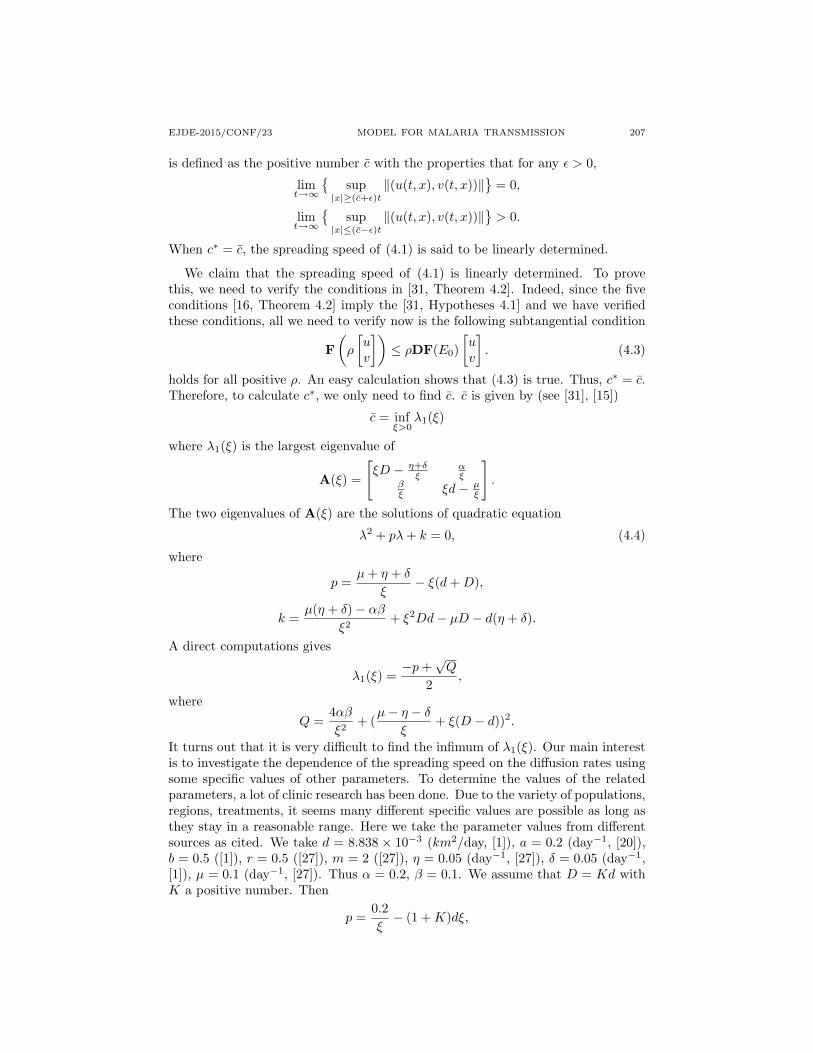
Our results imply that, as a steady state of the corresponding spatially-independentmodel, Ee is globally stable in the first quadrant. Figure 1 below is the graph of thenumerical solution with u(0) = 0.35 and v(0) = 0.05. From the graph we can seethat as t → ∞, (u(t), v(t)) → ( 1

3 ,14 ) = (ue, ve). In fact, when we choose different

initial values, we have the same scenario. That is, Ee = (ue, ve) is globally stable.Next we adjust the parameters. Recall that the meaning of b and r are mosquito-

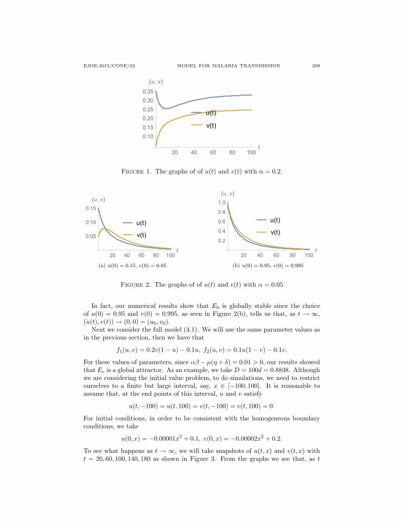
to-human and human-to-mosquito transmission efficiency, respectively. Small val-ues of b or r leads to small values of α or β. Without loss of generality, we assumethat α is decreased from 0.2 to 0.05 so that

αβ − µ(η + δ) = −0.05 < 0.

Thus the disease-free equilibrium E0 = (u0, v0) = (0, 0) is the only steady stateand our result shows that it is locally stable. Now we choose u(0) = 0.15 andv(0) = 0.05 to find the numerical solution. Figure 2(a) below is the graph of thesolution. We can see that, as t→∞, (u(t), v(t))→ (0, 0) = (u0, v0).


u(t)

v(t)

20 40 60 80 100t

0.10

0.15

0.20

0.25

0.30

0.35

{u, v }

Figure 1. The graphs of of u(t) and v(t) with α = 0.2.

u(t)

v(t)

20 40 60 80 100t

0.05

0.10

0.15

{u, v }

(a) u(0) = 0.15, v(0) = 0.05

u(t)

v(t)

20 40 60 80 100t

0.2

0.4

0.6

0.8

1.0

{u, v }

(b) u(0) = 0.95, v(0) = 0.995

Figure 2. The graphs of of u(t) and v(t) with α = 0.05

In fact, our numerical results show that E0 is globally stable since the choiceof u(0) = 0.95 and v(0) = 0.995, as seen in Figure 2(b), tells us that, as t → ∞,(u(t), v(t))→ (0, 0) = (u0, v0).

Next we consider the full model (4.1). We will use the same parameter values asin the previous section, then we have that

f1(u, v) = 0.2v(1− u)− 0.1u, f2(u, v) = 0.1u(1− v)− 0.1v.

For these values of parameters, since αβ − µ(η + δ) = 0.01 > 0, our results showedthat Ee is a global attractor. As an example, we take D = 100d = 0.8838. Althoughwe are considering the initial value problem, to do simulations, we need to restrictourselves to a finite but large interval, say, x ∈ [−100, 100]. It is reasonable toassume that, at the end points of this interval, u and v satisfy

u(t,−100) = u(t, 100) = v(t,−100) = v(t, 100) = 0.

For initial conditions, in order to be consistent with the homogeneous boundaryconditions, we take

u(0, x) = −0.00001x2 + 0.1, v(0, x) = −0.00002x2 + 0.2.

To see what happens as t → ∞, we will take snapshots of u(t, x) and v(t, x) witht = 20, 60, 100, 140, 180 as shown in Figure 3. From the graphs we see that, as t


becomes larger and larger, (u(t, x), v(t, x)) tends closer and closer to Ee = ( 13 ,

14 ).

This implies that Ee is a global attractor.

u(t,x)

v(t,x)

-100 -50 50 100x

0.05

0.10

0.15

0.20

0.25

{u, v }

(a) t = 20

u(t,x)

v(t,x)

-100 -50 50 100x

0.05

0.10

0.15

0.20

0.25

0.30

{u, v }

(b) t = 60

u(t,x)

v(t,x)

-100 -50 50 100x

0.05

0.10

0.15

0.20

0.25

0.30

{u, v }

(c) t = 100

u(t,x)

v(t,x)

-100 -50 50 100x

0.05

0.10

0.15

0.20

0.25

0.30

0.35{u, v }

(d) t = 140

u(t,x)

v(t,x)

-100 -50 50 100x

0.05

0.10

0.15

0.20

0.25

0.30

0.35{u, v }

(e) t = 180

Figure 3. The graphs of of u(t, x) and v(t, x) with α = 0.2

Conclusion. From our mathematical analysis of a model of malaria transmission,we see that when the basic reproduction number is less than one, the disease-freeequilibrium is the only equilibrium and it is locally asymptotically stable and ifthe reproduction number is greater than one, the disease-free equilibrium becomesunstable and an endemic equilibrium emerges and it is asymptotically stable. Wealso proved that, when the reproduction number is greater than one, there is aminimum wave speed c∗ such that for every c ≥ c∗, there exists a travelling wavesolution with wave speed c and the minimum wave speed is also the spreading speedof the disease. We also investigated the relationship between spreading speed and


diffusion coefficients. Our results show that when the infected mosquito populationequilibrates much faster than the human population, the spreading speed of thedisease is proportional to the square root of the human diffusive coefficient. Ingeneral situation, we only know that the movements of mosquito population andhuman population will speed up the spread of the disease. Therefore, when malariabreaks out in some regions, it is necessary to limit the movement of human beingto keep the spread of the disease under control. The exact relationship between thespreading speed and the diffusion coefficients need to be further investigated.

Acknowledgements. The authors would like to thank the anonymous refereesfor their valuable comments and suggestions and bringing reference [33] to ourattention. This work is partially supported by NSF grant DMS -1330801.

References

[1] M. Al-Arydah, R. Smith; Controlling malaria with indoor residual spraying in spatially het-

erogeneous environments, Mathematical Biosciences and Engineering, Vol. 8, No. 4, pp 889-914, 2011.

[2] L. J. S. Allen; An Introduction to Mathematical Biology, Prentice Hall, 2007.

[3] R. M. Anderson, R. M. May; Infectious Diseases of Humans: Dynamics and Control, OxfordUniversity Press, Oxford, UK, 1991.

[4] J. L. Aron; Mathematical modeling of immunity to malaria, Math. Biosci., 90 (1988), pp

385-396.[5] J. L. Aron, R. M. May; The population dynamics of malaria in The Population Dynamics

of Infectious Disease: Theory and Applications, R. M. Anderson, ed., Chapman and Hall,

London, 1982, pp 139-179.[6] N. Chitnis; Using Mathematical Models in Controlling the Spread of Malaria, Ph.D. thesis,

Program in Applied Mathematics, University of Arizona, Tucson, AZ, 2005.

[7] N. Chitnis, J. M. Cushing, J. M. Hyman; Bifurcation analysis of a mathematical model formalaria transmission, SIAM J. Appl. Math. Vol. 67. No. 1, 24-45, 2006.

[8] K. Dietz, L. Molineaux, A. Thomas; A malaria model tested in the African savannah, Bull.

World Health Organ., 50 (1974), pp 347-357.[9] B. Greenwood, T. Mutabingwa; Malaria in 2002. Nature, Vol. 415, 670-672, 2002.

[10] A. T. King, E. Mends-Brew, E. Osei-Frimpong, K. R. Ohene; Mathematical model for thecontrol of malaria-Case study: Chorkor polyclinic, Accra, Ghana, Global. Adv. Research J.

of Medicine and Medical Sci., Vol 1, No. 5, 108-118, 2012.

[11] J. C. Koella; On the use of mathematical models of malaria transmission, Acta Tropica, Vol.49, 1-25, 1991.

[12] J. C. Koella, R. Antia; Epidemiological models for the spread of anti-malarial resistance,

Malaria J., 2:3 (2003).[13] J. C. Koella, C. Boete; A model for the coevolution of immunity and immune evasion in

vector-borne disease with implications for the epidemiology of malaria, The American Natu-

ralist, 161 (2003), pp 698-707.

[14] A. Kolmogorov, I. G. Petrovsky, N. S. Piscounov; Etude de lequation de la diffusion aveccroissance de la quantite de matiere et son application a un probeme biologique, Bull. Moscow

Univ. Math. Mech., Vol. 1, 1-26, 1937.

[15] M. Lewis, J. Renclawowicz, P. V .D. Driessche; Traveling waves and spread rates for a westnile virus model, Bull. Math. Bio., Vol. 68, No. 1, pp 3-23, 2006.

[16] B. Li, H. Weinberger, M. Lewis; Spreading speeds as slowest wave speeds for cooperativesystems, Math. Biosci, Vol. 196, pp 82-98, 2005.

[17] J. Li, R. M. Welch, U. S. Nair, T. L. Sever, D. E. Irwin, C. Cordon-Rosales, N. Padilla;

Dynamic malaria models with environmental changes, in Proceedings of the Thirty-Fourth

Southeastern Symposium on System Theory, Huntsville, AL, 2002, pp 396-400.[18] Y. Lou, X. Zhao; A reaction-diffusion malaria model with incubation period in the vector

population, J. Math. Biol., 62 (2011), 543-568.[19] G. Macdonald; The Epidemiology and Control of Malaria, Oxford University Press, London,

1957.


[20] O. D. Makinde, K. O. Okosun; Impact of Chemo-therapy on Optimal ontrol of Malaria

Disease with Infected Immigrants, BioSystems, Vol. 104, 32-41, 2011.

[21] J. Nedelman; Introductory review: Some new thoughts about some old malaria models, Math.Biosci., 73 (1985), pp 159-182.

[22] G. A. Ngwa; Modelling the dynamics of endemic malaria in growing populations, Discrete

Contin. Dyn. Syst. Ser. B, 4 (2004), pp 1173-1202.[23] G. A. Ngwa, W. S. Shu; A mathematical model for endemic malaria with variable human

and mosquito populations, Mathematical and Computer Modeling, Vol. 32, 747-763, 2000.

[24] A. Okubo, S. Levin; Diffusion and Ecological Problems: Moderm Perspectives, Springer-Verlag, New York, 2002.

[25] O. Prosper, N. Ruktanonchai, M. Martcheva; Assessing the role of spatial heterogeneity and

human movement in malaria dynamics and control, J. Theor. Biol. Vol. 303, pp 1-14, 2012.[26] R. Ross; The Prevention of malaria, John Murray, London, 1911.

[27] S. Ruan, D. Xiao, J. C. Beier; On the delayed Ross-Macdonald model for malaria transmis-sion, Bull. of Math. Bio. Vol. 70, 1098-1114, 2008.

[28] J. Smoller; Shock waves and reaction-diffusion equations, Second Edition, Springer-Verlag,

1994.[29] S. T. Stoddard, A. C. Morrison, G. M. Vazquez-Prokopec, V. P. Soldan, T. J. Kochel, U.

Kitron, J. P. Elder, T. W. Scott; The Role of human movement in the transmission of

vector-borne pathogens. PLos Negl Trop Dis, 3(7):e481, 2009.[30] U. S. Global Health Policy, Fact Sheet, March 2011, The Henry J. Kaiser Family Foundation.

[31] H. F. Weinberger, M. A. Lewis, B. Li; Analysis of linear determinacy for spread in cooperative

models, J. Math. Biol., Vol. 45 (2002), 183-218.[32] M. E. Woolhouse, C. Dye, J. F. Etard, T. Smith, J. D. Charwood; Heterogeneities in the

transmission of infectious agents:implications for the design of control program. Proc. Natl.

Acad. Sci. USA, Vol. 94, 338-342, 1997.[33] C. Wu, D. Xiao; Travelling wave solutions in a non-local and time-delayed reaction-diffusion

model, IMA J. Appl. Math. Vol. 78, Issue 6(2013), 1290-1317.[34] H. M. Yang; Malaria transmission model for different levels of acquired immunity and

temperature-dependent parameters (vector), Revista de Saude Publica, 34 (2000), pp 223-

231.[35] H. M. Yang, M. U. Ferreira; Assessing the effects of global warming and local social and

economic conditions on the malaria transmission, Revista de Saude Publica, 34 (2000), pp

214-222.[36] Q. X. Ye, Z. Y. Li; Introduction to Reaction-Diffusion Equations, Science Press, Beijing,

China, 1994.

Zhenbu Zhang

Department of Mathematics and Statistical Sciences, Jackson State University, Jack-son, MS 39217, USA

E-mail address: [email protected]

Tor A. KwembeDepartment of Mathematics and Statistical Sciences, Jackson State University, Jack-

son, MS 39217, USAE-mail address: [email protected]

qualitative analysis of a mathematical model for …

Documents