QUADRATIC INTEGER PROGRAMMING APPROACH

FOR MRF-BASED LABELING PROBLEMS

Seong Jae Hwang

A THESIS

in

Robotics

Presented to the Faculties of the University of Pennsylvania in Partial

Fulfillment of the Requirements for the Degree of Master of Science in Engineering

2013

_______________________________

Camillo J. Taylor

Supervisor of Thesis

_______________________________

Camillo J. Taylor

Graduate Group Chairperson

ii

Contents

Acknowledgement ...................................................................................................... vii

Abstract ....................................................................................................................... viii

1. Introduction......................................................................................................... 1

2. Problem formulation .......................................................................................... 5

2.1 Labeling Problem .......................................................................................... 5

2.2 Graphical Models .......................................................................................... 6

2.3 Quadratic Programming ................................................................................ 8

2.4 MRF to QIP ................................................................................................... 10

2.5 Penalty Function ............................................................................................ 13

2.6 Smoothness Function ..................................................................................... 14

2.7 The Choice of and ................................................................................... 18

2.8 Label Constraints ........................................................................................... 20

3. Algorithm ............................................................................................................. 24

4. OpenGM .............................................................................................................. 31

iii

4.1 Problem Models ............................................................................................. 32

4.1.1 Inpainting ............................................................................................. 33

4.1.2 Multiclass Color-based Segmentation .................................................. 34

4.1.2 Color Segmentation .............................................................................. 35

4.1.3 Object-based Segmentation .................................................................. 35

4.1.5 MRF Photomontage .............................................................................. 35

4.1.6 Stereo Matching .................................................................................... 36

4.1.6 Image Inpainting ................................................................................... 37

4.1.7 Chinese Character ................................................................................. 37

4.1.9 Scene Decomposition ........................................................................... 37

4.1.10 Non-rigid Point Matching ................................................................... 38

4.2 Inference Methods ......................................................................................... 38

4.2.1 Message Passing ................................................................................... 39

4.2.2 Graph Cut ............................................................................................. 40

5. Experiment .......................................................................................................... 43

5.1 OpenGM ........................................................................................................ 43

5.2 HDF5 ............................................................................................................. 44

5.3 Scoring Matrix Construction ..................................................................... 45

5.4 Results ........................................................................................................... 46

5.5 The QIP Analysis .......................................................................................... 56

6. Conclusion ........................................................................................................... 59

iv

List of Tables

Table 5-1. Problem models with properties. ................................................................ 43

Table 5-2. Algorithms with short descriptions and function types .............................. 44

Table 5-3. Inference methods used on problem models. ............................................. 45

Table 5-4. color-seg results. ......................................................................................... 49

Table 5-5. color-seg-n4 results. ................................................................................... 49

Table 5-6. color-seg-n8 results. ................................................................................... 49

Table 5-7. dtf-chinesechar results. ............................................................................... 50

Table 5-8. inpainting-n4 results. .................................................................................. 50

Table 5-9. inpainting-n8 results. .................................................................................. 50

Table 5-10. matching results. ....................................................................................... 51

Table 5-11. mrf-inpainting results. .............................................................................. 51

Table 5-12. mrf-photomontage results. ........................................................................ 51

v

Table 5-13. mrf-stereo results. ..................................................................................... 52

Table 5-14. object-seg results. ..................................................................................... 52

Table 5-15. scene-decomposition results. .................................................................... 52

vi

List of Figures

Figure 5-1. HDF5 file structure .................................................................................. 47

Figure 5-2. Examples of dtf-chinesechar results using QIP ....................................... 54

Figure 5-3. Examples of inpainting-n4 using TRWS-LF2 and QIP. .......................... 54

Figure 5-4. Examples of color-seg-n4 using TRWS-LF2 and QIP. ........................... 55

Figure 5-5. Examples of mrf-stereo using QIP. .......................................................... 56

vii

Acknowledgement

I would like to thank Prof. Camillo J. Taylor for supervising this research which is large-

ly based on the current research under his guidance. I would also like to thank Prof.

Kostas Daniilidis and Prof. Jean Gallier for serving on the thesis committee and being

supportive.

viii

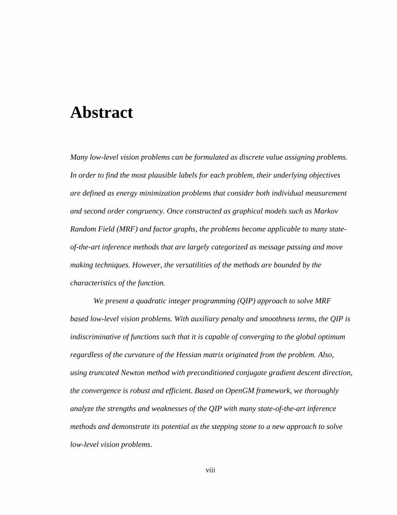
Abstract

Many low-level vision problems can be formulated as discrete value assigning problems.

In order to find the most plausible labels for each problem, their underlying objectives

are defined as energy minimization problems that consider both individual measurement

and second order congruency. Once constructed as graphical models such as Markov

Random Field (MRF) and factor graphs, the problems become applicable to many state-

of-the-art inference methods that are largely categorized as message passing and move

making techniques. However, the versatilities of the methods are bounded by the

characteristics of the function.

We present a quadratic integer programming (QIP) approach to solve MRF

based low-level vision problems. With auxiliary penalty and smoothness terms, the QIP is

indiscriminative of functions such that it is capable of converging to the global optimum

regardless of the curvature of the Hessian matrix originated from the problem. Also,

using truncated Newton method with preconditioned conjugate gradient descent direction,

the convergence is robust and efficient. Based on OpenGM framework, we thoroughly

analyze the strengths and weaknesses of the QIP with many state-of-the-art inference

methods and demonstrate its potential as the stepping stone to a new approach to solve

low-level vision problems.

1

1. Introduction

Many computer vision problems focus on extracting low-level information, such as stereo

correspondence or clustering, from images. Also known as early vision problems, these

low-level problems often require pixel-wise accuracy and spatial correlation among

nearby pixels. Such measurements allow the problems to be formulated as energy

minimization problems that capture both demands with two different energy functions:

one measures the pixel-wise cost such as intensity difference and the other assesses

relationship among neighbors such as smoothness. When these functions take discrete

values, the energy function can effectively represent various low-level problems. For

instance, in clustering problem, the labels indicate the assigned clusters of pixels, and in

stereo problem, they are intensity differences of each pixel from two images. Such

discrete energy minimization problems pose a major merit of also being able to be

expressed as a graphical model, Markov Random Field (MRF) [12], allowing various

inference methods to be applicable.

MRF model opened the doors to many powerful inference methods, and their

successful performances on various problems are well known [34]. However, the distinct

energy functions used in the different methods made the comparison among those

algorithms inconvenient. In 2006, [34] built a unifying framework providing a fair

comparison among many prominent inference algorithms at the time such as graph cut

2

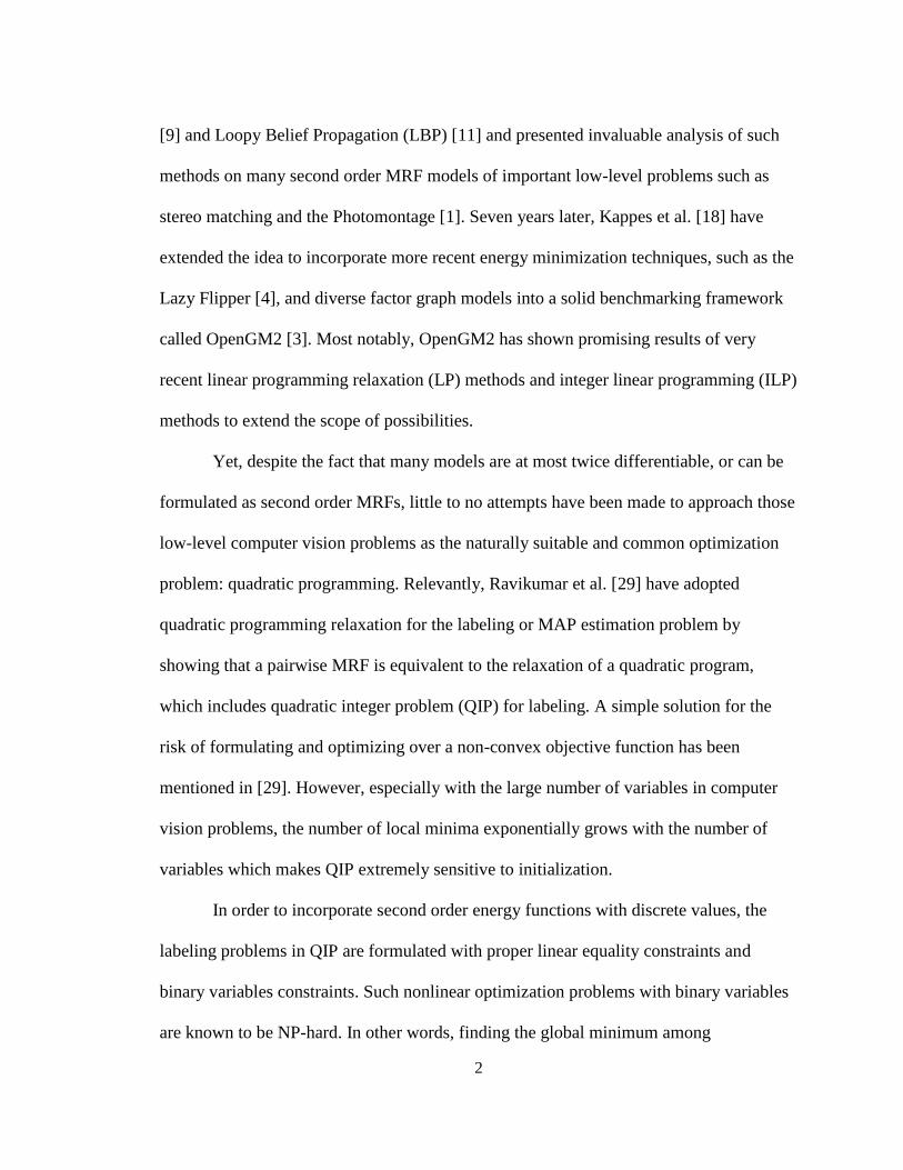
[9] and Loopy Belief Propagation (LBP) [11] and presented invaluable analysis of such

methods on many second order MRF models of important low-level problems such as

stereo matching and the Photomontage [1]. Seven years later, Kappes et al. [18] have

extended the idea to incorporate more recent energy minimization techniques, such as the

Lazy Flipper [4], and diverse factor graph models into a solid benchmarking framework

called OpenGM2 [3]. Most notably, OpenGM2 has shown promising results of very

recent linear programming relaxation (LP) methods and integer linear programming (ILP)

methods to extend the scope of possibilities.

Yet, despite the fact that many models are at most twice differentiable, or can be

formulated as second order MRFs, little to no attempts have been made to approach those

low-level computer vision problems as the naturally suitable and common optimization

problem: quadratic programming. Relevantly, Ravikumar et al. [29] have adopted

quadratic programming relaxation for the labeling or MAP estimation problem by

showing that a pairwise MRF is equivalent to the relaxation of a quadratic program,

which includes quadratic integer problem (QIP) for labeling. A simple solution for the

risk of formulating and optimizing over a non-convex objective function has been

mentioned in [29]. However, especially with the large number of variables in computer

vision problems, the number of local minima exponentially grows with the number of

variables which makes QIP extremely sensitive to initialization.

In order to incorporate second order energy functions with discrete values, the

labeling problems in QIP are formulated with proper linear equality constraints and

binary variables constraints. Such nonlinear optimization problems with binary variables

are known to be NP-hard. In other words, finding the global minimum among

3

exponentially many local minima quick requires impractical amount of computation as

the problem size grows. Also, enforcing binary variables alters the objective function to

be more concave, leaving the problem to be more vulnerable to initialization.

Nonetheless, Murray et al. [26] showed the possibility of obtaining the global minimum

in a pool of local minima using smoothness function. Consequently, the convex

smoothness function carefully dominates the concave terms to make the entire objective

function convex, paving descent paths towards the global minimum regardless of the

starting position. Their results were encouraging compared to other mixed-integer

nonlinear programming problem solvers.

In this paper, we present a QIP method for solving the labeling problems in low-

level computer vision. The labeling problems that we are interested in can easily be

formulated as pairwise MRF models, which are identical to QIP problems [29]. We have

used the factor graph models provided in OpenGM2 [3] to express QIP objective

functions. More specifically, only the second order problems were considered because of

the nature of QIP, but we were neither limited by function types nor grid structures. Then

we introduce smoothness terms to make the problem convex and use a descent method to

search for the global minimum. Since many of the problems of our interests are large in

terms of number of variables, we used truncated Newton method with preconditioned

conjugate gradient direction. Despite the immense sizes of the objective matrices (n from

1,000 to1,000,000), the algorithm took reasonable computation time to converge due to

the sparse block structure of the objective matrices. Using OpenGM2 benchmark, we

show our results compared to other state-of-the-art methods in terms of quality and speed.

4

In the following sections, we provide thorough problem formulation. In chapter 2,

we describe the basic problem formulation, including the transition from labeling

problem to QIP and the integration of auxiliary penalty and smoothness terms.

Furthermore, we mention truncated Newton method with precondition conjugate gradient

because this is the fundamental basis to our optimization scheme. Then, in chapter 3, we

present the algorithm in depth along with the analysis. In chapter 4, we give detailed

descriptions of OpenGM framework. The experiments to compare our algorithm among

various other state-of-the-art algorithms various problem models based on OpenGM2

framework will be demonstrated in chapter 5. Lastly, in chapter 6, we conclude with the

future work.

5

2. Problem formulation

In this chapter, we first describe the basic knowledge necessary to understand the

problem. Then we transition into the formulation of the labeling problem into a quadratic

integer programming problem.

2.1 Labeling Problem

Many of the low-level vision problems can be understood as assigning a discrete value to

each pixel to represent relevant information. For instance, in image segmentation

problems of partitioning image into sets, each pixel is labeled to indicate the superpixel it

is partitioned into. In stereo problems of finding pixel correspondences between two

images, the distance between the corresponding pixels is translated as labels. Naturally,

to measure the quality of the assignments of each pixel independently with respect to the

problem objectives, first order function arise in each problem to compute what we call

matching costs. In addition, the problems also imply certain level of spatial continuity

among pixels to reflect the coherence of the objects in the image. To express such

constraints, higher order functions inevitably appear to assess the agreement of a pixel

given other pixels, usually its neighbors, and return what we call smoothness costs. Given

6

a set of pixels and a label space , for each pixel with label , written as ,

we can express the total cost as an energy function

( ) ( ) ( )

(1)

where is the matching cost and ( ) is the smoothness cost. While

are often defined explicitly to define the basic goal of the problem, ( ) can be

completely arbitrary and affect the quality of the result. For instance, in a color based

segmentation problem, considering 4 (2 horizontal and 2 vertical) and 8 (2 horizontal, 2

vertical, and 4 diagonal) neighbors shows different results. Also, the functions sometimes

possess certain conditions for some algorithms such as -expansion [9] that requires the

function to be metric. Thus, the choice of smoothness function needs to be carefully

considered for both the algorithms and the models. Our algorithm only requires the

smoothness function to be of at most second order while it is not restricted to be metric.

2.2 Graphical Models

Given a set of nodes V and a set of edges E, a graph G = (V, E) can be used to express the

dependence among variables, and a graph with a set of undirected edges is also called a

Markov Random Field (MRF). Then, the inference problem comes down to assigning the

most probable label for each node, or finding the maximum a posteriori (MAP)

estimation. Let be a variable for node and the set of those variables be

. Since we are interested in a pairwise MRF, we consider the functions related

to the set of edges , and let be a parameter and be a potential function

7

between two nodes and that are connected by an edge . Without loss of

generality, as shown in [35], the joint probability distribution of a generic MRF is

proportional to a pairwise MRF such that

(∑ ∑ ( )

) (2)

where is the set of parameters and the first summation consists of parameters and func-

tions related to individual variables. Therefore, the MAP problem finds that maximiz-

es (2), which is

∑ ∑ ( )

(3)

We mention another graphical model that is used throughout the experiments. A

factor graph consists of a set of variable nodes , a set of factor nodes ,

and a set of edges that makes G a bipartite graph. To define the variable

nodes involved with each factor , let | be the neigh-

borhood of a factor and the variable nodes in that neighborhood be . Then each

factor has an associated function which we can use to express the ener-

gy function for a set of labels as

∑

(4)

Using (4), the MAP solution to the log-linear model is

8

∑

(5)

which is the set of most likely labels. The OpenGM framework specifically modeled the

problems using factor graph instead of MRF because the relationship between functions

and variables can be expressed more intuitively than what MRF can represent [20].

2.3 Quadratic Programming

An optimization problem where its objective function is a quadratic function subject to

linear constraints is called a quadratic programming (QP). For , ( is the

space of symmetric space of size n) and , a general QP formulation is

(6)

where , , and . If is positive definite, various opti-

mization methods such as conjugate gradient method become suitable. We modify (6) to

enforce the variables to be integers such that

(7)

9

where the last constraint requires the variables to be binary. However, the last constraint

not only is nonlinear, but also makes the problem NP-hard; thus the problem is relaxed

into

(8)

where for the simplicity, an inequality of a vector and a constant implies the element-

wise inequality, and this can be solved in polynomial time with applied heuristic

schemes to obtain integer results (Chapter 7 on [14]). Also known as quadratic integer

programming (QIP), (7) only allows binary variables, but the problem can be formulated

to fully express the energy functions that take discrete values, or labels, given a factor

graph and its functions, which will be discussed next.

2.4 MRF to QIP

Our algorithm solves the QIP relaxation representation of the labeling problems, which

are in MRFs; thus, it is important to show their equivalence [29]. We first introduce

indicator functions to imply discrete values such that

{

, ( ) {

, (9)

where and are discrete values, or labels. (9) can be used to explicitly express the po-

tential functions as

10

∑

( ) ∑ ( )

which allow us to write (3) without expressing edges as

∑ ∑ ( )

(10)

where is the parameter associated with variable with label , and is the pa-

rameter associated with and with labels and respectively. The replacement of

edges with the new potential functions allows (10) to be represented in a relaxed linear

programming (LP) form as shown in [5]. First, the integer linear programming (ILP)

formulation of (11) is

∑ ∑

∑

∑

where the variables and ( ) are the relaxations

of (10). The second and the fourth constraints enforce the variable to have only one

11

label, and the first and the third constraints imply the binary AND relationship between

and . Similar to (8), the above ILP is relaxed into

∑ ∑

∑

∑

(11)

The binary indicator functions in (9) can be interpreted as an independent joint between

two unary indicator functions such that ( ) ( ), which implies that

the relaxed variables can also be understood such that .

Now we can rewrite (11) as

∑ ∑

∑

which is a relaxed QP. In [29], they have shown that the optimal value of the relaxed ver-

sion is equal to the optimal value of the (10), which is the MAP problem of a MRF model.

12

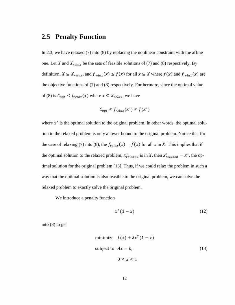
2.5 Penalty Function

In 2.3, we have relaxed (7) into (8) by replacing the nonlinear constraint with the affine

one. Let and be the sets of feasible solutions of (7) and (8) respectively. By

definition, , and for all where and are

the objective functions of (7) and (8) respectively. Furthermore, since the optimal value

of (8) is where , we have

where is the optimal solution to the original problem. In other words, the optimal solu-

tion to the relaxed problem is only a lower bound to the original problem. Notice that for

the case of relaxing (7) into (8), the for all in . This implies that if

the optimal solution to the relaxed problem, is in , then

, the op-

timal solution for the original problem [13]. Thus, if we could relax the problem in such a

way that the optimal solution is also feasible to the original problem, we can solve the

relaxed problem to exactly solve the original problem.

We introduce a penalty function

(12)

into (8) to get

(13)

13

where and . In order to minimize (12) with a positive

coefficient, each variable is pushed towards either 0 or 1. With a sufficiently large , the

benefit of reducing the penalty term dominates benefit of using continuous variables

, and the variables become binary, or . Also, we also notice that the ad-

dition of the penalty function does not affect the optimal value of (13) compared to the

original problem because (12) is zero for a binary given a sufficiently large . Thus, the

optimal values are the same for the newly relaxed problem (13) and the original problem

(7); thus, the optimal solutions to both problems are the same. Since having a zero penal-

ty from (12) enforces the relaxed and the original problem to have the same global mini-

mum, (12) is called an exact penalty function [26, 13].

However, even though the global minimizers for (7) and (13) are the same, find-

ing one is challenging because (12) is highly concave, and with sufficiently large , the

entire objective function becomes concave. Thus, while it excels at finding a local mini-

mum, having one that is also the global minimum becomes a whole new task. This leads

to introducing another term in the next section.

2.6 Smoothness Function

Many smoothing methods attempt to help finding the global minimum for a problem with

numerous local minima by “smoothing” out relatively insignificant local minima. In the

context of optimization [17], the objective function is modified appropriately to suppress

the magnitudes of higher order derivatives while preserving the general structure. One

way is by locally smoothing the function, making the function more resilient to numerical

14

noise, which may cause many undesirable minima that could mislead searching methods

away from desired local minima. Unfortunately, this solution could be irrelevant when

the problem does not suffer from reaching meaningful local minima successfully such as

the problem of our interest. Thus, a smoothing method covering the larger scope of the

problem called global smoothing is suggested.

The goal of global smoothing is to tweak the function to find the global minimum

out of many local minima. By definition, a function is strictly convex if there is only one

minimum, which is the global minimum. Thus, we appropriately modify the objective

function to be strictly convex. Again, by appropriately we mean without losing the fun-

damental nature of the function, so the global minimizer of the smoothed function still

resembles of the original function. The objective function with a smoothing term is

thus

for an objective function and a smoothing parameter . The choice of the

smoothing function is crucial along with the parameter, and Theorem 3.1 in [26] provides

an important insight that guarantees the existence of a smoothing function, which in the

context of the binary problem is a twice-differentiable function with a positive definite

Hessian, with a large enough . Then, a local minimum of the smoothed function found

by a minimization method is in fact the global minimum.

However, even though the minimizer is heading towards the global minimum, it is

still not the same as that of the original function. Thus, this technique is used iteratively

to reinforce the weakness of the original problem, which is the extreme dependence on

15

the initialization. A large is used initially to find the roughest but the safest minimizer

that attempts to find a good minimizer regardless of the quality of the initialization. Then,

the next iteration uses a smaller to reduce the amount of smoothness to start reverting

back to the original problem and the minimizer of the previous iteration, which is much

closer to the correct local minimizer than a generalized initialization. Eventually, be-

comes zero and the smoothness is disappeared, and by then the local minimizer found

using the original non-convex objective function is optimistically the same as the global

minimum. Consequently, is the parameter to consider in each iteration, and the mecha-

nism of choosing a good is not trivial. If is too large, the smoothness term could

overwhelm the problem structure so the minimizer could be biased towards optimizing

the smoothness term. On the other hand, if is too small, the weak smoothness function

could start introducing local minima. Thus, should be delicately chosen in order to get

the most out of smoothing while avoiding the oversimplification of the problem.

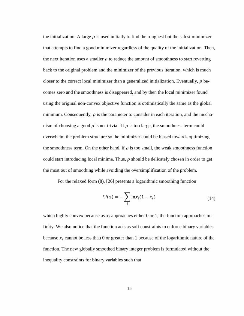
For the relaxed form (8), [26] presents a logarithmic smoothing function

∑

(14)

which highly convex because as approaches either 0 or 1, the function approaches in-

finity. We also notice that the function acts as soft constraints to enforce binary variables

because cannot be less than 0 or greater than 1 because of the logarithmic nature of the

function. The new globally smoothed binary integer problem is formulated without the

inequality constraints for binary variables such that

16

∑

(15)

Such technique of implying inequality constraints is called a barrier method and (14) is

an example of a barrier function known as a logarithmic barrier function. Now we see

that (14) is an amalgamation of ∑ and ∑ , which are the basic logarithmic

barrier functions for inequalities and respectively. Although eliminating in-

equality constraints does simplify the problem to our favor, the primary advantage of us-

ing a logarithmic barrier function is using its strict convex nature for smoothing. Thus,

combining (13) with (14), we have the final problem formulation that incorporates both

the concave penalty function and the convex smoothing function:

∑

(16)

Thus, the problem is shaped by two parameters, and . We have already

pointed out that the penalty term does not affect the structure of the original problem. The

choice of the smoothing function prevails such that it also does not bias the variables to

favor 0 or 1 because (14) is an even function with respect to the point of minimum, which

occurs when the variable is 0.5. Thus, even with sufficiently large and , optimization

techniques on (16) still finds the minimizer based on the structure, or the gradient, of the

original objective function while the additional terms only assist the process. Since

we have acknowledged that the additional terms are independent of the original functions,

17

we now notice that the choice of and is a whole new question, which dictates the suc-

cess of our algorithm.

2.7 The Choice of and

The meaning of sufficiently large penalty function parameter can be arbitrary, but

based on the original problem, can be cleverly chosen. As stated in 2.5, the purpose of

the penalty function is to adjust the problem to be concave, which enforces the minimizer

to be at the boundary of the feasible space. This can be achieved with an adequately large

, but if is too large the penalty term can overwhelm the structure of the original

function. So ideally, one wants to be just enough to make the objective concave,

preserving the general shape of the original function.

We focus on the relevant case of binary QIP. We mention that a second-order

function is concave if its Hessian is negative semidefinite, or has eigenvalues that are less

than or equal to zero. Keeping this in mind, we can rewrite (13) with a quadratic function

such that

(17)

which can be rewritten as

18

(18)

where is an identity matrix of the size of . Clearly, the Hessian of the objective func-

tion of (18) is . Since is symmetric, its eigenvalues are real. Assuming is not

negative semidefinite, let be the largest positive eigenvalue of . The largest eigenval-

ue of is then . Since , choosing will ensure the largest eigenval-

ue to be less than or equal to zero, making safely negative semidefinite.

Thus, the smallest and the most ideal is the largest eigenvalue of . This is allows us to

take out of the consideration, simplifying the algorithm to manipulate only the smooth-

ness parameter . The remaining portion of the penalty function, , does not affect

the choice of so its absence is indifferent, resulting the equation

Choosing a good value for the smoothing parameter , however, can be more

complicated. Initially, it can be sufficiently large to induce overall convexity of the func-

tion. As the algorithm progresses, the value decreases to start revealing local minima as

the function becomes non-convex. Once the function is not convex anymore, its behavior

gets difficult to measure since the function in each iteration differ by the degree of non-

convexity dictated purely by the , which has no analytical insight below a certain value.

19

In [26], they have heuristically chosen a constant for the initial for all their experiments

that diminishes by a constant factor, which is heuristically determined as well.

In our algorithm, different from [26], we only consider in each iteration. De-

spite the heuristics, we point out the fact the algorithm can be terminated when the varia-

bles are not exactly 0 or 1 given the nature of the labeling constraints. As a result, is not

required to converge very close to 0 as the algorithm converges to satisfying conditions

beforehand. This is based on the problem structure, which will be explained in the next

section.

2.8 Label Constraints

The problem of our particular interest is the labeling problem, which can be formulated

as

∑

(19)

which includes the smoothness function as well. Based on the structure of the first con-

straint, this binary QIP can be turned into a labeling problem that can support any label.

Without loss of generality, assume the original objective matrix agrees with the in-

stance we are about to state. Let be the number of variables considered in the given

problem such as number of pixels. Let be the number of labels. We say that a varia-

ble has a label by letting be a binary vector of size by 1 where only the var-

iable is 1. Since only one label can be assigned to each , the constraint is

20

∑

(20)

where is the element of . The idea of (20) is equivalent to the first constraint of

(11) which consists of an indicator function. We can simplify (20) for each such that

The list of equality constraints can be reconstructed as follows. Let the vector of

size . The objective function variable is a vector of size such that

In other words, is a stack of for all such that

(21)

Finally, a matrix of size by is constructed such that

where is the element of at row and column . Thus, is matrix that contains

for the corresponding in to obey (20), and we can formulate (20) as

(22)

In all our labeling problem formulation in QIP, we assume the equality constraints follow

the structure of (22).

We point out another trick to simplify (19). We first rewrite the smoothness func-

tion as

21

∑

∑

(23)

Notice that in (23), the left summation implies the constraint . If this constraint ex-

ists, then (22) implies that because the individual sum has to equal to 1 as in (21).

Also, since the left summation of (23) is a convex function itself, the right summation of

(23) can be taken out such that the final QIP formulation becomes

∑

(24)

Note that we cannot consider the same simplification using the right summation of (23)

because itself and (22) do not imply . We notice that the new smoothing function

does make the variables to be biased towards 1. However, the labeling problem concerns

with which variable is assigned a value instead of what value is assigned. Since the

smoothing function does not discriminate the variables, the simplification of the penalty

function is safe.

22

3. Algorithm

When applicable, second-order optimization techniques such as Newton method are

accepted as better approaches than first-order optimization techniques, and they become

more appealing when the Hessian matrix can be found effortlessly. Fortunately, the QIP

formulation allows us to extract the Hessian matrix very easily. However, the type of

problems we are interested in, which are low-level vision problems, consists of thousands

of variables, and with high number of labels, the size of the scoring matrix can be

quickly have a size of a million by a million. For this reason, optimization techniques that

require matrix inversion become impractical. Furthermore, matrix computation of

involving such large matrix should be a concern, but due to the block sparse structure of

the Hessian matrix, which will be described in the next section, matrix multiplication can

be efficiently handled. As in [26], we utilize truncated Newton method, which find a

negative descent direction using conjugate gradient method instead of a matrix inversion.

To avoid matrix inversion, we first turn the problem into an unconstrained prob-

lem by merging the constraints into the objective function. In short, given (24), we start

with a constraint obeying initial variable such that and consider the direction

that does not violate the constraint. We let be a vector of where is the number

of labels, and the direction lives in the null space of defined such that . Let

be a matrix of rank that its column vectors are that basis of the null space of

23

such that . Then, we can safely compute by searching for the vector of size

such that . Since we know the structure of , we used constructed

the Householder reflection matrix of vector of size with the first element added by

√ in the direction of to get a reflection that negates all the elements of except the

first one to be zero. Thus, we form the null space by using all the columns except for the

first column of the Householder reflection matrix as the basis, creating the null space .

We compute for using and express such that where is the feasible

step. The null space will be used in almost every matrix multiplication involving . For

instance, a reduced Hessian matrix is computed and used instead of to perform

multiplications involving in terms of . Also, this process needs to be done only once

before the main iteration because does not change given the problem.

Before the iteration, given of size by where for number of la-

bels and number of variables, we assign by finding the largest eigenvalue of . Find-

ing the exact value of the maximum eigenvalue of by solving the characteristic poly-

nomial is ideal, but this quickly becomes impractical as the size of the matrix increases to

thousands. Since any greater than or equal to the maximum eigenvalue of is still ac-

ceptable, we used the Gershgorin circle theorem to estimate the upper bound of the max-

imum eigenvalue. In our experiments, we have observed this to be viable.

The gist of a linesearch method is finding the step direction. In standard Newton

method, the search direction is where is the Hessian matrix and is the

first-order gradient. However, as mentioned previously, inverting a large size Hessian

matrix is not suitable for the problem of interest. Thus, in truncated Newton method, the

search direction is found approximately by using conjugate gradient method (CG). Com-

24

pared to a normal gradient method of finding the search direction orthogonal to the cur-

rent direction, CG computes the step orthogonal to the current vector with respect to the

Hessian matrix. The conjugate direction is much more efficient than the standard gradient,

enough to justify the extra computation, which involves a matrix multiplication of the

large size Hessian matrix. However, CG is still an iterative method that guarantees its

convergence in steps, and this requires a special attention since the size of our Hessian

is very large. Fortunately, the number of steps can be vastly reduced if the condition

number of the Hessian matrix is small. That is, if the differences among the eigenvalues

are small, the Hessian matrix is shaped spherically, often allowing CG to converge well

before steps. Various preconditioning techniques exist to find a preconditioning matrix

that approximates such that can be computed efficiently where the

condition number of is much smaller than that of . For a large scale matrix, such

as our case, a simple diagonal preconditioning is used where we use the diagonal of the

Hessian matrix as the preconditioner. Clearly, this technique is effective when the matrix

is non-singular, which is not always the case for our reduced Hessian matrix. Thus, we

incorporated a commonly used Levenberg-Marquardt method on the reduced Hessian

matrix by adding a diagonal matrix of entries to reduce the trust region.

Before we explain the conjugate gradient search direction, we first explicitly show

the necessary components to demonstrate the simplicity of constructing them. First, we

rewrite (24) such that

25

where is the objective function of (24). Given , we can express in terms of

such that it is the null space of , or for a vector of size as

∑

(25)

where is the row of . Thus, if is computed, then the problem can be formulated

as an unconstrained QIP as

. (26)

The first-order derivative of (25) with respect to can easily derived as

where

for . Notice (25) is equivalent to .

Finally, the second-order derivative of (25) with respect to is

and we mention that .

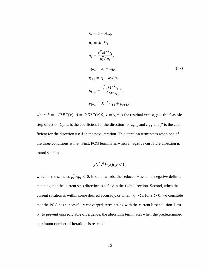
Now that we have all the necessary components, let us illustrate the precondi-

tioned conjugate gradient (PCG) method as in [31], but in terms of our variables. In our

case, PCG tries to solve

at each of its iteration for such that . Given an appropriate preconditioner

, the entire PCG procedures is as follows:

26

(27)

where , , , is the residual vector, is the feasible

step direction , is the coefficient for the direction for and and is the coef-

ficient for the direction itself in the next iteration. This iteration terminates when one of

the three conditions is met. First, PCG terminates when a negative curvature direction is

found such that

which is the same as . In other words, the reduced Hessian is negative definite,

meaning that the current step direction is safely in the right direction. Second, when the

current solution is within some desired accuracy, or when | | for , we conclude

that the PCG has successfully converged, terminating with the current best solution. Last-

ly, to prevent unpredictable divergence, the algorithm terminates when the predetermined

maximum number of iterations is reached.

27

The PCG is a direction searching method for the truncated-Newton method,

which is an iterative method itself. The truncated-Newton method, once it converges and

finds a local minimum, is repeated with the minimizer of the previous iteration for the

current iteration that is closer to the original problem by gradually decreasing the

smoothness parameter . For our experiments, a constant coefficient is mul-

tiplied to such that . The entire algorithm terminates if each that consists

in such way as in (22) is assigned a label with enough confidence such that

for where . Note that does not need to be very close to 1, es-

pecially with large labels. In practice, we used . Otherwise, the algorithm termi-

nates after a certain number of top iterations. Once the final solution in binary variables is

chosen, the index of the maximum variable in each for is the label for the

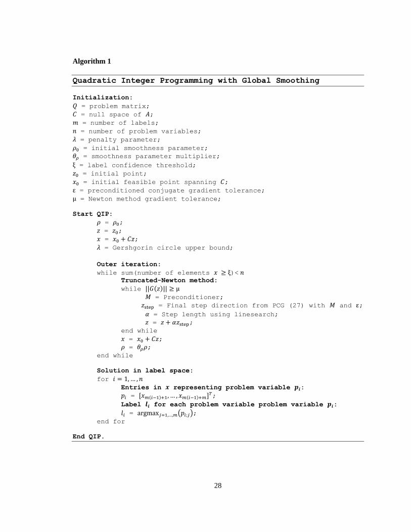
respective such that ( ). The pseudo-code of our entire algo-

rithm is presented on the next page.

28

Algorithm 1

Quadratic Integer Programming with Global Smoothing

Initialization:

= problem matrix;

= null space of ;

= number of labels;

= number of problem variables;

= penalty parameter;

= initial smoothness parameter; = smoothness parameter multiplier;

= label confidence threshold;

= initial point;

= initial feasible point spanning ;

= preconditioned conjugate gradient tolerance;

= Newton method gradient tolerance;

Start QIP:

= ;

= ;

= ;

= Gershgorin circle upper bound;

Outer iteration:

while sum(number of elements )< Truncated-Newton method:

while || ||

= Preconditioner; = Final step direction from PCG (27) with and ;

= Step length using linesearch; = ; end while

= ; = ; end while

Solution in label space:

for Entries in representing problem variable :

= ;

Label for each problem variable problem variable :

= ( ); end for

End QIP.

29

4. OpenGM

Fortunately for the community, Andres, Beier, and Kappes have provided an extensive

framework that is based upon a C++ template library called OpenGM [3] that formulates

discrete graphical models and implements inference techniques on those models. As

mentioned in 2.2, various low level computer vision problems are posed in factor graphs,

and they are stored as HDF5 [16] files that follows unified conventions and describes the

problem exactly with minimal information. As a result, the inference algorithms do not

need to necessarily know the problems. In fact, many of the inference methods have been

incorporated into OpenGM by creating wrappers for the pre-existing codes that are

available by the individual authors to interpret and use the HDF5 files. However, even

though the simplification of the modeling scheme greatly benefits the overall framework

in many ways, we believe that we need to understand the problems on a high level in

order to truly identify the strengths and weaknesses of each algorithm. Thus, we dig a

little deeper into the models to better understand existing low level vision problems and

analyze them in terms of our algorithm, which allows us to explain the bridge between

the models and QIP formulation. Also, for our research, it is equally important to

comprehend the cores of the inference methods to select the ones that have similar

limitations as ours to provide a fairer and more common stage.

30

4.1 Problem Models

Many of the low level vision problems have been constructed in various researches to

facilitate the computer vision community. Since the problems have originally been

formulated for individual algorithm, they have been reformulated as factor graphs in

HDF5 files with unified convention. On the high level, the models are derived from

common low level vision problems such as segmentation and stereo problems that

involve single or multiple images and assignment of each pixel with a problem related

label. On the low level, the entire factor graph can be constructed with basic parameters

such as number of variables and the predetermined scoring functions that describe the

problems. We go over suitable problem models from both high and low level

perspectives.

By the nature of computer vision problems involving images, many models in-

volve tens of thousands of variables to represent each pixel in the image. To distinguish

these variables from the QIP variables, we will call them the problem variables. Also, we

will be talking about the problems that are implemented in OpenGM. The smallest and

the largest problem sizes are 19 and 7 million respectively. Typically, the problem size

affects the runtime of the algorithms proportionally. For instance, in QIP, the problem

size is directly correlated to the size of the objective matrix. More specifically, letting

be the number of problem variables, the size of is proportional to .

On a high level sense, the label space represents the objective of the problem. For

example, in a segmentation problem, the label space is the number of maximum super-

pixels. Varying from 2 to 100,000, the number of labels also has a similar effect as the

31

problem size such that the size of is exactly . Therefore, the size of can in-

crease very quickly, giving a practical limitation in terms of the number of variables and

labels that QIP can handle reasonably. Fortunately, we do not need to make any assump-

tion about the label space as it is provided and static for each model.

An arguably more significant component of the problem models is the order of

functions. Although the factor graph is capable of implementing higher order functions,

many low level problems use second order functions. This is because the problems often

deal with the grid structured 2D images and consider neighboring pixels, which makes

second order function appropriate. The majority of the models in OpenGM are defined

with second order functions, which fit perfectly for our QIP method along with many

other state-of-the-art techniques that only support up to second order functions.

As mentioned in the introduction, low level vision problems handle tasks that are

closer to the raw image than the semantic representation for high level techniques such as

machine learning. Consequently they may look relatively simpler than the high level

tasks, but the difficulty and the significance are nonetheless complex and invaluable.

4.1.1 Inpainting [10]

The inpainting problem is a problem of filling in the missing portion of the image. The

original image consists of a three equally divided pie chart shape where the label space

has 3 labels, each for a different color and 1 label for the background boundary to

maintain the circular shape. To human eyes, the most plausible picture comes intuitively

based on the given portion of the image. In other words, the nearby pixels are naturally

32

factored in to make the most sense possible. The solution is not so obvious, especially for

convex relaxation solvers because of the multiple global minima that exist as a result of

indistinguishable labels. The problem is of an intermediate size with a medium number of

problem variables and four labels. Also, the Potts function based on pairwise factor is

used, favoring algorithms that require second order functions and metric distances. Two

types of models exist that consider 4 neighbors (n4) and 8 neighbors (n8). Overall, the

algorithms have performed well, some of them achieving the global minimum.

4.1.2 Multiclass Color-based Segmentation [8]

One of the most common low level vision problems, segmentation is a problem of

mapping each pixel to a much smaller sized disjoint sets. This particular partitioning

problem is color based, relying on pixel intensities to make the decision. Also, each

image focuses on an object rather than a scene with multiple objects. Thus, purpose is

more towards image simplification rather than object or scene recognition. Naturally, the

4 neighbor and 8 neighbor versions are provided with the predetermined colors as the

label space of size from 4 to 12 and the problem size in the order of 5. Also, the second-

order Potts function make it a well applicable problem. Roughly speaking, the

performance deviation among different algorithm is small but not many of them have

reached the optimal results.

33

4.1.2 Color Segmentation [2]

Similar to 4.1.2, this color segmentation problem uses small to large images from an

order of 4 to 6 with fewer labels. The notable difference is that the images contain

multiple objects with distinct colors, and with only 3 to 4 classes to partition into, the

segments tend to be those significantly distinct objects, making them look more intuitive

to human eyes than 4.1.2. Thus, based on an 8 neighbor Generalized Potts function of

order 2, this segmentation problem is one of the easier models to solve as many

algorithms have performed very well on average.

4.1.3 Object-based Segmentation [32]

Each label represents an object such as grass, tree, or sky, and the problem is to assign an

appropriate label to each pixel based on its 4 nearby pixels. The main difference between

4.1.3 and 4.1.4 is the potential function. 4.1.4 uses various parameters to incorporate

shape-texture, color, and location along with a second order Potts function to formulate a

more complex energy function. However, since the HDF5 files already contains every

possible outcome of the function, the inference methods do not need to compensate

anything. This problem is also one of the easier problems.

34

4.1.5 MRF Photomontage [1]

Photomontage consists of two problems that involve multiple images. The first model is

the well-known panorama stitching where multiple overlapping images merge into one

image in a spatially agreeable manner. The second model is group photo merging

[Szeliski] where multiple images take from the same camera pose with slight variations

in the contents combine together using the most plausible portion of those images into a

single image. The problem sizes are in the order of 5. The label represents which image

the pixel is from, where the numbers of images are 5 and 7. Using the second-order Potts

function, the problem is extremely difficult that the performances varied significantly

among different algorithms due to the complexity of the images and the large problem

size.

4.1.6 Stereo Matching [34]

Given two rectified images that are horizontally shifted, the stereo correspondence

problem is to find a disparity map to show the horizontal displacement of every pixel

from one image to the other. Naturally, close objects will have higher disparities than the

distant objects. The label space is the pixel distance between the two corresponding pixel,

varying from 16 to 60. The problem variable size is in an order of 6, alarming that the

problem size is on the larger side of the spectrum. Each instance of the problem uses the

second-order version of either a truncated L1 or a truncated L2 functions. Both functions

35

obey the triangular inequality in terms of the label differences, making it a difficult but

applicable problem.

4.1.6 Image Inpainting [11]

Similar to 4.1.1, this problem solves to fill in the missing region of a noisy image.

However, compared to 4.1.1, the problem is much more complicated. The label space is

not predetermined to be an arbitrary number. Instead, the label space is of size 256

representing the pixel intensity. A second-order truncated L2 function is used assuming 4

neighbor grid structure. In general, because of the large label space, the inference

algorithms had the longest runtime and the least success rate of all the problem models.

4.1.7 Chinese Character [27]

Originated from the KAIST Hanja2 database, this is another inpainting problem where

the images are handwritten binary Chinese characters. Even though the problem size is

relatively small with only binary labels, the potential function is explicitly learned via

decision trees based on 300 training images which considered 8 horizontal and vertical

neighbors and 27 farther neighbors. Thus, the function does not imply metric distance,

allowing only a small number of inference methods including our algorithm to be

applicable.

36

4.1.9 Scene Decomposition [15]

Fundamentally, this is another segmentation problem, but the problem formulation is

different from the other segmentation problems we have. The problem variables are

superpixels of size 100 to 200 with 8 possible labels. The unary potential function is a

mixture of various features such as SIFT features. The pairwise potential function is

based on the gradient magnitudes along the edges separating the superpixel and its 4

neighboring superpixels. Thus, the overall potential function is explicit, preventing the

use of metric distance based inference methods. If solvable, the problem is very easy

considering the small problem size and small label space where the algorithms have

consistently achieved the global optimum very fast.

4.1.10 Non-rigid Point Matching

This problem does not involve 2D images. Instead, it is a bipartite matching problem

between two sets of size 19 or 20. Naturally, the label space is the node label. The one-to-

one constraint has been implied with large diagonal entries in the scoring tables, and the

edge weights are expressed with binary potential functions. Despite the simplicity, the

problem is extremely difficult as the performances among the techniques vary greatly. In

some cases, the lower bound could be calculated, but the verified optimality could never

be achieved.

37

4.2 Inference Methods

The strength of OpenGM is its unified framework that integrates various state-of-the-art

inference methods. The algorithms have been modified with wrappers to adapt the

structured syntax and semantics of OpenGM problem models. Thus, every inference

method can be used to solve every model. The only limitation is the algorithm’s inherent

inability to solve certain types of problems. The overall runtime has been sacrificed in

general, but the amount is modest and easily justified by the adaptability of the

framework. For the purpose of this research, we have chosen the methods that have

similar requirements, namely the problem size and the function order. The algorithms

take vastly distinctive approaches from each other that it is worth understanding them.

4.2.1 Message Passing

This type of algorithms, as self-explanatory it is, passes massages between the connected

nodes in a graph. Ultimately, the algorithms attempt to assign a value to each variable to

make the most sense that maximizes a MAP formulation given the dependencies with

predetermined weights between nodes. A common message passing algorithm is Belief

Propagation [28] which solves the exact solution if the graph is an undirected acyclic

graph, or a tree. For a graph with cycles, Loopy Belief Propagation (LBP) is used to

consider the possibility of not converging as in [11]. A more effective way to deal with

loops was presented by Wainwright et al. [36] called tree-reweighted message passing

(TRW). It solves trees within the graph that are connected by edges with weights to

38

obtain a probability distribution of trees, and since it is a formulated as a dual problem,

TRW also finds a lower bound, which is not guaranteed to increase consistently. Thus,

TRW also does not always guarantee convergence. Kolmogorov [22] has demonstrated a

way to avoid decreasing the lower bound using a modified version of TRW called

sequential TRW (TRW-S). The success rate of these algorithms are impressive, but the

thorough consideration of every single possible state of the graph makes them

computationally challenging with large number of variables. In terms of the labeling

problem, the potential functions do not need to be metric or nonnegative, making them

more applicable than many other algorithms. Both MRF-LIB [33] and libDAI [25]

versions of these message passing algorithms have been implemented in OpenGM.

4.2.2 Graph Cut

The graph cut algorithms of our interest are -expansion [9] and -swap [9]. These two

very popular and successful algorithms make moves that lower the energy after each

move. In the each iteration of -expansion, the move is an assignment of a label to the

variables are not already assigned as which lowers the energy, and in the each iteration

of -swap, some of the variables with label are assigned as and vice versa in a way

that lowers the energy, and they terminate when there are no moves that lowers the

energy for each . The moves are chosen by solving min-cut problems; hence they are

categorized as graph cut algorithms. Since min-cut problems can be solved in polynomial

time and the rest of the algorithms are simple, they are generally very fast. However, to

solve the min-cut problem efficiently in polynomial time, the potential functions have to

39

be metric and semi-metric for -expansion and -swap respectively. For labels and ,

the function is called a semi-metric if it satisfies and

is equivalent to . For labels , , and The function is a metric if it is semi-

metric and follows the triangle inequality . As a result, the

graph cut methods were only applied to the problem models that met those requirements.

But if applicable, the algorithms are capable of providing fast and accurate results.

OpenGM provides implementation of -expansion and -swap from two libraries:

boost graph library [21] and MRF-LIB [33].

A linear programming primal-dual extension of a move making algorithm is pre-

sented by Komodakis et. al [23]. By the nature of duality, a lower bound is also computed.

The potential functions need to be at least semi-metric to guarantee optimality, and the

solution is equivalent to that of -expansion if the function is metric. However, the algo-

rithm is still bottlenecked by the complexity of min-max problem. The modified version

called FastPD [24] achieved noticeable increase in speed while not compromising the

quality. If applicable, FastPD converged the fastest in all the problems while obtaining

near optimal solutions.

Another algorithm is mentioned here that relies on min-max problem. Quadratic

pseudo-boolean optimization (QPBO) is presented by Boros and Hammer [7] for uncon-

straint quadratic binary programming and network-flow problems based on roof duality.

This algorithm has been applied to graphical models [30], and OpenGM constructs the

problem as a min-max problem. QPBO has been used to solve the Chinese character

problem which is a general second-order binary model.

40

For some of the inference methods we have mentioned so far, a post-processing

technique called the Lazy Flipper [4] has been applied. It is a binary version of Iterated

Conditional Modes (ICM) [6], which iteratively performs greedy search. The Lazy

Flipper is a more generalized version of ICM that flips binary variables in terms of

subsets instead of just single variables. Since the solution is improved iteratively from an

initial state, the algorithm is heavily dependent on the initialization. Thus, the Lazy

Flipper was used as a post-processing step that is applied on the results of the previously

mentioned algorithms to improve the solution.

41

5. Experiment

In this section, we show the experiment results of state-of-the-art inference methods and

our method on various low vision problems. We use OpenGM to run the previously

mentioned inference algorithms in 4.2 and our algorithm on the problems in 4.1. The

entire experiment was run on an Intel i7-2670QM at 2.20GHz PC with 8 GB RAM

running on 64 bit Linux with MATLAB 2013. All the computations were given a single

thread with at most 3 out of 4 cores running at the same time.

While QIP converges to local minim, there tends to be rooms for improvements in

our results compared to the state-of-the-art methods. However, we want to point out that

the primary purpose of our research is to introduce the potential of a new technique to

approach low level vision problems. As we have observed in our experiments, we have

seen ways to improve the solution, which will be discussed later in this section.

5.1 OpenGM

The latest version of OpenGM and its manual can be found in [3]. The framework

already contains many of the inference methods, but it still requires many third party

codes and binaries from different websites. For this experiment, HDF5 can be

downloaded from the website [16]. In terms of the inference methods, a shell script is

42

given for Linux environment to automatically download and patch the necessary external

libraries. Some methods, such as FastPD, need to be downloaded separately from their

respective websites and then patched to be functional. A cross platform compiler CMake

[19] is used to conveniently build the entire project. Currently, OpenGM is more

conveniently handled on Linux so we highly recommend setting up OpenGM on Linux.

The more detailed process is described in the manual.

Linux shell scripts are provided to run the suitable methods on the problems.

Since there are many algorithms, each with parameters to specify the function type, we

have provided a table listing all the algorithms of different function types with descrip-

tions that were used in the experiments in Table 5.1. Also, to have a better look at the ap-

plicability of the algorithms on the models, Table 5.2 is included to show the methods

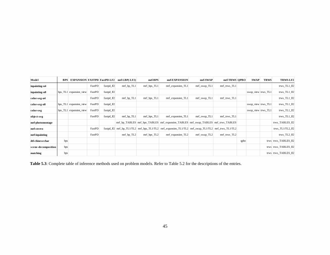
used on the problems in terms of Table 5.3.

5.2 HDF5

All the necessary models can be obtained from the OpenGM website, and third party

programs exist to graphically view the content of HDF5 file format. We used the built-in

HDF5 toolbox in MATLAB to read and use the files for QIP. As we have stated before,

the advantage of using HDF5 format is the simplicity which comes from the implicit

convention. Thus, in order to utilize the models, it is important to

43

Table 5.1: Complete table of models with properties. In the Functions column, Explicit (Potts) indicate that the model fully consists of explicit

functions and the Potts functions are expressed explicitly as a part of the explicit functions.

Model Variables Labels Order Structure Q matrix structure Functions Instances

inpainting-n4 14400 4 2 grid 4 5 banded Explicit (Potts) 2

inpainting-n8 14400 4 2 grid 8 9 banded Explicit (Potts) 2

color-seg-n4 76800 3 - 12 2 grid 4 5 banded Explicit (Potts) 9

color-seg-n8 76800 3 - 12 2 grid 8 9 banded Explicit (Potts) 9

color-seg 21000 - 414720 3,4 2 grid 8 9 banded Explicit, Potts 3

object-seg 68160 41372 2 grid 4 5 banded Explicit, Potts 5

mrf-photomontage 425632 - 514080 41401 2 grid 4 5 banded Explicit (Potts) 2

mrf-stereo ~100000 16, 20, 60 2 grid 4 5 banded Explicit, TL1, TL2 3

mrf-inpainting 21838 - 65536 256 2 grid 4 5 banded Explicit, TL2 2

dtf-chinesechar 4992 - 17856 2 2 sparse non-banded Explicit 100

scene-decomposition 150 - 208 8 2 sparse non-banded Explicit 715

matching 19 - 21 19 - 21 2 full non-banded Explicit 4

44

Table 5.2: Complete list of algorithms with descriptions

Algorithms (detailed) Algorithm Algorithm description Function type

bps BPS Sequential Belief Propagation TABLES

bps_TL1 BPS Sequential Belief Propagation TL1

expansion_view EXPANSION alpha-Expansion VIEW

FastPD FASTPD FastPD

fastpd_lf2 FastPD-LF2 FastPD with Lazy Flipper

mrf_bp_TABLES mrf-LBP MRF-LIB Loopy Belief Propagation TABLES

mrf_bp_TL1 mrf-LBP-LF2 MRF-LIB Loopy Belief Propagation TL1

mrf_bp_TL2 mrf-LBP-LF2 MRF-LIB Loopy Belief Propagation TL2

mrf_bps_TABLES mrf-BPS MRF-LIB Sequential Belief Propagation TABLES

mrf_bps_TL1 mrf-BPS MRF-LIB Sequential Belief Propagation TL1

mrf_bps_TL2 mrf-BPS MRF-LIB Sequential Belief Propagation TL2

mrf_expansion_TABLES mrf-EXPANSION MRF-LIB alpha-Expansion TABLES

mrf_expansion_TL1 mrf-EXPANSION MRF-LIB alpha-Expansion TL1

mrf_expansion_TL2 mrf-EXPANSION MRF-LIB alpha-Expansion TL2

mrf_swap_TABLES mrf-SWAP MRF-LIB alpha-beta-Swap TABLES

mrf_swap_TL1 mrf-SWAP MRF-LIB alpha-beta-Swap TL1

mrf_swap_TL2 mrf-SWAP MRF-LIB alpha-beta-Swap TL2

mrf_trws_TABLES mrf-TRWS MRF-LIB Sequential Tree-reweighted TABLES

mrf_trws_TL1 mrf-TRWS MRF-LIB Sequential Tree-reweighted TL1

mrf_trws_TL2 mrf-TRWS MRF-LIB Sequential Tree-reweighted TL2

qpbo QPBO Quadratic Pseudo-Boolean Optimization

swap_view SWAP alpha-beta-Swap VIEW

trws TRWS Sequential Tree-reweighted TABLES

trws_TABLES_lf2 TRWS-LF2 Sequential Tree-reweighted and Lazy Flipper TABLES

trws_TL1 TRWS Sequential Tree-reweighted TL1

trws_TL1_lf2 TRWS-LF2 Sequential Tree-reweighted with Lazy Flipper TL1

trws_TL2_lf2 TRWS-LF2 Sequential Tree-reweighted with Lazy Flipper TL2

45

Table 5.3: Complete table of inference methods used on problem models. Refer to Table 5.2 for the descriptions of the entries.

Model BPS EXPANSION FASTPD FastPD-LF2 mrf-LBP(-LF2) mrf-BPS mrf-EXPANSION mrf-SWAP mrf-TRWS QPBO SWAP TRWS TRWS-LF2

inpainting-n4 FastPD fastpd_lf2 mrf_bp_TL1 mrf_bps_TL1 mrf_expansion_TL1 mrf_swap_TL1 mrf_trws_TL1 trws_TL1_lf2

inpainting-n8 bps_TL1 expansion_view FastPD fastpd_lf2 swap_view trws_TL1 trws_TL1_lf2

color-seg-n4 FastPD fastpd_lf2 mrf_bp_TL1 mrf_bps_TL1 mrf_expansion_TL1 mrf_swap_TL1 mrf_trws_TL1 trws_TL1_lf2

color-seg-n8 bps_TL1 expansion_view FastPD fastpd_lf2 swap_view trws_TL1 trws_TL1_lf2

color-seg bps_TL1 expansion_view FastPD fastpd_lf2 swap_view trws_TL1 trws_TL1_lf2

object-seg FastPD fastpd_lf2 mrf_bp_TL1 mrf_bps_TL1 mrf_expansion_TL1 mrf_swap_TL1 mrf_trws_TL1 trws_TL1_lf2

mrf-photomontage mrf_bp_TABLES mrf_bps_TABLES mrf_expansion_TABLES mrf_swap_TABLES mrf_trws_TABLES trws_TABLES_lf2

mrf-stereo FastPD fastpd_lf2 mrf_bp_TL1/TL2 mrf_bps_TL1/TL2 mrf_expansion_TL1/TL2 mrf_swap_TL1/TL2 mrf_trws_TL1/TL2 trws_TL1/TL2_lf2

mrf-inpainting FastPD mrf_bp_TL2 mrf_bps_TL2 mrf_expansion_TL2 mrf_swap_TL2 mrf_trws_TL2 trws_TL2_lf2

dtf-chinesechar bps qpbo trws trws_TABLES_lf2

scene-decomposition bps trws trws_TABLES_lf2

matching bps trws trws_TABLES_lf2

46

fully understand the structure of the files. Since the convention is not conspicuous at first,

we have included Figure 5.1 to help understand and visualize the structure.

5.3 Scoring Matrix Construction

Based on the understanding of 5.2, we can construct the scoring matrix for our

algorithm. Following the convention, we can obtain a predetermined scoring table of

size by representing a potential function . Given two problem variables with

labels and , we let vectors and be the binary vectors of size that have zeros for

entries and ones at for and for . In other words, the index of one of each vector

represents its label. Then, is the output of the function with labels and such

that .

As seen in the factors vectors of the HDF5 files, each problem variable is as-

signed with a number to refer to that variable, or node, with. We first initialize the scor-

ing matrix as a zero matrix of size by . Then for each factor, we know the vari

ables involved, let them be and , along with the appropriate scoring table of size

by . Now, we create our own convention by constructing such that

for and of each factor. The final scoring matrix is created by adding and the trans-

pose of to make it symmetric and divide it by 2 because . In other

words, consists of blocks of scoring tables that are responsible for the appropriate en-

tries of the vector as we have stated in (22). Thus, the sparsity of is correlated to the

47

…

function index

function type

function order

variable 1

variable 2

… …

function order

table size 1

table size 2

…

…

table entry 1

table entry 2

table entry 3

table entry 4

…

…

table size 1

table size 2

…

…

parameter 1

parameter 2

… 2

0

number of variables

number of factors

number of function types

function id 1

number of tables

function id 2

number of tables

2

1

…

number of labels

…

factors

HDF5

function-id-16000

(explicit function)

indices

values

function-id-1600x

(non-explicit function)

indices

values

header

states

Figure 5.1: HDF5 file structure

48

complexity of the factor graph. For instance, the grid-structured problems create as 5-

banded and 9-banded block matrix structures for 4 neighbors and 8 neighbors grid struc-

tures respectively. Considering the number of problem variables being much larger than

the label space, the matrices are usually very sparse. Even for those problems that do not

have grid structures, they are still highly sparse. Such sparse nature of allows QIP to be

applicable with large problems. In terms of memory, storing the sparse matrices, espe-

cially with the repeating potential functions, can be extremely efficient. The computation

can be optimized with block-wise matrix multiplication.

5.4 Results

The results of the total of 2808 experiments of solving 850 small to large problem

instances with various inference methods are summarized on tables from Table 5.4 to

Table 5.15. The best column shows the percentage of the solutions that were the best

among all the algorithms, while the ver. opt column shows the percentage of the duality

gaps that were within the tolerance of and verified the global optimality.

Throughout the experiments, the QIP used , , , ,

, and used a vector of zeros as the initial point . The penalty parameter was

estimated with the Gershgorin upper bound. The visual results based on the OpenGM

scripts are provided in Figure 5.1 through 5.4.

We first observe the results from the perspective of the models. The difficulties of

the problems have been revealed by the outcomes of the inference methods. While the

verified optimality could be found consistently for some problems such as object

49

Table 5.4: color-seg (3 instances)

algorithm mean runtime mean value mean bound best ver. opt

FastPD 0.50 sec 308472275.00 ∞ 66.67% 0.00%

mrf-BPS 158.63 sec 308733349.67 ∞ 0.00% 0.00%

EXPANSION 9.73 sec 308472275.67 ∞ 66.67% 0.00%

FastPD-LF2 23.78 sec 308472275.00 ∞ 66.67% 0.00%

SWAP 9.95 sec 308472292.33 ∞ 66.67% 0.00%

TRWS 207.15 sec 308472310.67 308472270.43 66.67% 33.33%

TRWS-LF2 213.97 sec 308472294.33 308472270.43 66.67% 33.33%

QIP 218.90 sec 308487641.33 ∞ 0.00% 0.00%

Table 5.5: color-seg-n4 (9 instances)

algorithm mean runtime mean value mean bound best ver. opt

FastPD 0.37 sec 20034.80 ∞ 0.00% 0.00%

FastPD-LF2 9.48 sec 20033.21 ∞ 0.00% 0.00%

mrf-LBP-LF2 61.64 sec 20053.25 ∞ 0.00% 0.00%

mrf-BPS 39.21 sec 20094.03 ∞ 0.00% 0.00%

mrf-EXPANSION 1.40 sec 20033.45 ∞ 0.00% 0.00%

mrf-SWAP 0.98 sec 20050.50 ∞ 0.00% 0.00%

TRWS 39.78 sec 20012.18 20012.14 88.89% 77.78%

TRWS-LF2 77.76 sec 20012.17 20012.14 88.89% 77.78%

QIP 207.32 sec 27514.79 ∞ 0.00% 0.00%

Table 5.6: color-seg-n8 (9 instances)

algorithm mean runtime mean value mean bound best ver. opt

FastPD 0.87 sec 20011.14 ∞ 0.00% 0.00%

BPS 138.76 sec 20120.79 ∞ 0.00% 0.00%

EXPANSION 13.55 sec 20011.13 ∞ 0.00% 0.00%

FastPD-LF2 41.71 sec 20010.28 ∞ 0.00% 0.00%

SWAP 16.06 sec 20038.26 ∞ 0.00% 0.00%

TRWS 165.91 sec 19991.39 19991.16 33.33% 22.22%

TRWS-LF2 221.79 sec 19991.27 19991.16 100.00% 22.22%

QIP 202.43 sec 28140.54 ∞ 0.00% 0.00%

50

Table 5.7: dtf-chinesechar (100 instances)

algorithm mean runtime mean value mean bound best ver. opt

BPS 105.68 sec −49537.08 ∞ 68.00% 0.00%

QPBO 0.15 sec −49501.95 −50119.38 6.00% 0.00%

TRWS 132.36 sec −49496.84 −50119.41 4.00% 0.00%

TRWS-LF2 115.79 sec −49519.44 −50119.41 32.00% 0.00%

QIP 3.28 sec -49452.04 ∞ 0.00% 0.00%

Table 5.8: inpainting-n4 (2 instances)

algorithm mean runtime mean value mean bound best ver. opt

FastPD 0.02 sec 454.75 ∞ 50.00% 0.00%

FastPD-LF2 0.30 sec 454.75 ∞ 50.00% 0.00%

mrf-LBP-LF2 6.46 sec 475.56 ∞ 50.00% 0.00%

mrf-BPS 2.82 sec 454.35 ∞ 100.00% 0.00%

mrf-EXPANSION 0.02 sec 454.75 ∞ 50.00% 0.00%

mrf-SWAP 0.02 sec 454.35 ∞ 100.00% 0.00%

mrf-TRWS 2.92 sec 490.48 448.09 50.00% 50.00%

TRWS-LF2 6.17 sec 489.30 448.09 50.00% 50.00%

QIP 5.84 sec 499.91 ∞ 0.00% 0.00%

Table 5.9: inpainting-n8 (2 instances)

algorithm mean runtime mean value mean bound best ver. opt

FastPD 0.13 sec 465.02 ∞ 100.00% 0.00%

BPS 8.62 sec 468.21 ∞ 50.00% 0.00%

EXPANSION 0.49 sec 465.02 ∞ 100.00% 0.00%

FastPD-LF2 1.03 sec 465.02 ∞ 100.00% 0.00%

SWAP 0.40 sec 465.02 ∞ 100.00% 0.00%

TRWS 11.52 sec 500.09 453.96 50.00% 0.00%

TRWS-LF2 11.72 sec 499.30 453.96 50.00% 0.00%

QIP 6.43 sec 496.99 ∞ 0.00% 0.00%

51

Table 5.10: matching (4 instances)

algorithm mean runtime mean value mean bound best ver. opt

BPS 0.33 sec 40.26 ∞ 25.00% 0.00%

TRWS 0.31 sec 64.29 15.22 0.00% 0.00%

TRWS-LF2 1.06 sec 32.38 15.22 75.00% 0.00%

QIP 26.47 sec 37500000119.86 ∞ 0.00% 0.00%

Table 5.11: mrf-inpainting (2 instances)

algorithm mean runtime mean value mean bound best ver. opt

FastPD 10.45 sec 32939430.00 ∞ 0.00% 0.00%

mrf-LBP-LF2 819.54 sec 26597364.50 ∞ 0.00% 0.00%

mrf-BPS 827.27 sec 26612532.50 ∞ 0.00% 0.00%

mrf-EXPANSION 66.37 sec 27248297.50 ∞ 0.00% 0.00%

mrf-SWAP 156.89 sec 27392252.00 ∞ 0.00% 0.00%

mrf-TRWS 760.51 sec 26464865.00 26462450.59 0.00% 0.00%

TRWS-LF2 3604.92 sec 26463829.00 26462450.59 100.00% 0.00%

Table 5.12: mrf-photomontage (2 instances)

algorithm mean runtime mean value mean bound best ver. opt

mrf-LBP 1351.45 sec 438611.00 ∞ 0.00% 0.00%

mrf-BPS 449.70 sec 2217579.50 ∞ 0.00% 0.00%

mrf-EXPANSION 13.15 sec 168226.00 ∞ 100.00% 0.00%

mrf-SWAP 15.20 sec 197706.00 ∞ 0.00% 0.00%

TRWS 390.74 sec 1243144.00 166827.07 0.00% 0.00%

TRWS-LF2 666.65 sec 735193.00 166827.12 0.00% 0.00%

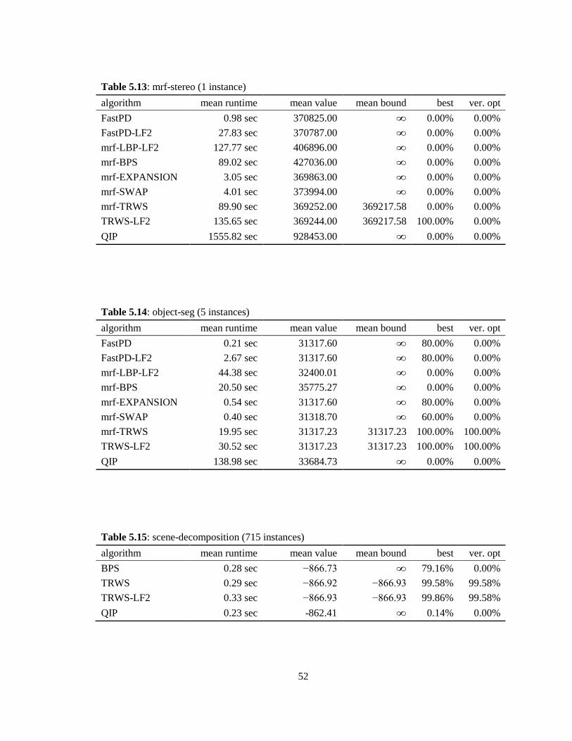
52

Table 5.13: mrf-stereo (1 instance)

algorithm mean runtime mean value mean bound best ver. opt

FastPD 0.98 sec 370825.00 ∞ 0.00% 0.00%

FastPD-LF2 27.83 sec 370787.00 ∞ 0.00% 0.00%

mrf-LBP-LF2 127.77 sec 406896.00 ∞ 0.00% 0.00%

mrf-BPS 89.02 sec 427036.00 ∞ 0.00% 0.00%

mrf-EXPANSION 3.05 sec 369863.00 ∞ 0.00% 0.00%

mrf-SWAP 4.01 sec 373994.00 ∞ 0.00% 0.00%

mrf-TRWS 89.90 sec 369252.00 369217.58 0.00% 0.00%

TRWS-LF2 135.65 sec 369244.00 369217.58 100.00% 0.00%

QIP 1555.82 sec 928453.00 ∞ 0.00% 0.00%

Table 5.14: object-seg (5 instances)

algorithm mean runtime mean value mean bound best ver. opt

FastPD 0.21 sec 31317.60 ∞ 80.00% 0.00%

FastPD-LF2 2.67 sec 31317.60 ∞ 80.00% 0.00%

mrf-LBP-LF2 44.38 sec 32400.01 ∞ 0.00% 0.00%

mrf-BPS 20.50 sec 35775.27 ∞ 0.00% 0.00%

mrf-EXPANSION 0.54 sec 31317.60 ∞ 80.00% 0.00%

mrf-SWAP 0.40 sec 31318.70 ∞ 60.00% 0.00%

mrf-TRWS 19.95 sec 31317.23 31317.23 100.00% 100.00%

TRWS-LF2 30.52 sec 31317.23 31317.23 100.00% 100.00%

QIP 138.98 sec 33684.73 ∞ 0.00% 0.00%

Table 5.15: scene-decomposition (715 instances)

algorithm mean runtime mean value mean bound best ver. opt

BPS 0.28 sec −866.73 ∞ 79.16% 0.00%

TRWS 0.29 sec −866.92 −866.93 99.58% 99.58%

TRWS-LF2 0.33 sec −866.93 −866.93 99.86% 99.58%

QIP 0.23 sec -862.41 ∞ 0.14% 0.00%

53

segmentation and scene decomposition by duality methods, the global optimum could not

be achieved at all for many problems such as matching and mrf-stereo. Also, although the

large problems such as mrf-stereo tend to be more difficult compared to the small prob-

lems such as scene decomposition, this is not always true. For instance, as seen on Table

5.10, the bipartite matching problem of size ~20 variables and ~20 possible labels is the

smallest sized problem but the results had a very high deviation and the optimality could

not be verified. The runtime, however, was proportional to the size of the problem. The

one-to-one relationship was implied with the potential functions with extremely high di-

agonal values as the soft constraints, but the QIP could not accomplish one-to-one rela-

tionship. The conjecture is that once the QIP has made an initialization which is not one-

to-one, then climbing back up the current descent direction to more optimal locations be-

comes immensely difficult with diagonal values that are practically close to infinity. The

applicable methods were limited for the models with non-metric potential functions, but

the problem complexities were indifferent of the function types as we see that Table 5.10

and Table 5.15 were challenging and moderate respectively in terms of the difficulties.

We would like to point out the fact that for mrf-stereo problem, we have only used the

smallest instance out of the three available because the QIP has not been optimized to yet

handle the other two problem sizes. The Photomontage was the most difficult problem in

terms of the quality and the runtime of the solution such that the best and the worst solu-

tions differed by an order of one. Also, the inpainting problem 4.1.7 and the Photomon-

tage problem 4.1.5 create very large scoring matrices for the QIP because of the large

number of problem variables and the label space. Thus, the current version of QIP could

not be used to solve those problems in this experiment.

54

Figure 5.2: Examples of dtf-chinesechar results. Top row: Given images of Chinese letters with

missing portions. Bottom row: QIP results of the respective top images.

Figure 5.3: Examples of inpainting-n4 and inpainting-n8 results. Top row: inpainting-n4 results.

From left to right: TRWS-LF2 and QIP for plain ring, TRWS-LF2 and QIP for inverse ring. Bot-

tom row: inpainting-n8 results. From left to right: TRWS-LF2 and QIP for plain ring, TRWS-LF2

and QIP for inverse ring.

55

Figure 4: Examples of color-seg-n4 results. Left column: TRWS-LF2. Right column: QIP

56

Figure 5.5: Examples of mrf-stereo results. Top: ground truth disparity map. Bottom: QIP results

disparity map.

57

We immediately observe that TRW-S from either MRF-LIB or boost graph li-

brary was the most versatile inference method as it was applied to all the problem models

regardless of the function types. Except for the Photomontage models, TRW-S provided

one of the best solutions while also yielding the lower bounds. However, the quality of

the results came with the cost of slow runtime. Naturally, the Lazy Flipper extended

TRW-S (TRWS-LF2) could be applied to all the problems which usually improved the

results of TRW-S. The biggest improvement could be observed on the matching problem

on Table 5.10 where the mean value of TRW-S was halved with the Lazy Flipper. TRW-

S struggled to reduce the duality gap for the Photomontage problem, which TRWS-LF2

reduced but could not overcome the poor initialization. On the side, we could verify the

quality of the lower bound by realizing the duality gap of -expansion. Belief Propaga-

tion (BPS) methods also prevailed in all the models, resulting excellent mean values. In

general, BPS was slightly faster and higher results than TRW-S. In terms of the computa-

tional speed, FastPD came out on top of all the algorithms when applicable. On average

for most of the experiments, FastPD converged in less than one second when other meth-

ods required minutes. Although the results were not always optimal, the solutions were

consistently impressive, often achieving the best solutions. The Lazy Flipper was imple-

mented on FastPD on some models to improve the results at the cost of computation time.

We could also observe two very similar move making methods which are -expansion

and -swap. On our experiments, -expansion had slightly better results than -swap.

Such outcome was expected because -expansion requires metric potential functions

compared to -swap that requires the less strict semi-metric potential functions. Since

58

all the applicable problems had metric functions, -swap could not utilize its versatility

of handling semi-metric functions.

5.5 The QIP Analysis

As observed in the tables, the current version of QIP often struggled to find the

competitive results compared to the other state-of-the-art inference methods depending

on the difficulties of the problems. However, that does not mean that QIP is incapable of

converging to the global optimum. The scene-decomposition instances are relatively

small sized with 150 to 208 problem variables with 8 labels. Despite the size, the problem

consists of non-metric potential functions, immediately limiting many algorithms

requiring metric or semi-metric potential functions for guaranteed convergence. The QIP

achieved the verified global optimum on the problem instance 0102234. The exact same

standard parameter values were used for all the problem models and instances. When we

altered the

parameter values to those that were better for each problem instance, our solutions were

often improved.

The QIP heavily relies on the strength of smoothness term determined by the pa-

rameter . For the most experiments, the results appear to be on the right track towards

the global minima as they close to the better solutions. Ideally, assuming the current point

is in the right direction, the parameter should be just enough to reveal the correct trajecto-

ry while still smoothing out misleading local minimizers. However, the current tuning

scheme is optimistically heuristic as we reduce it by an arbitrary . Increasing

59

to take more conservative steps did not improve the quality of the results by a considera-

ble amount. We suspect that with numerous seemingly appealing local minima in the

problems, the QIP makes very close calls when it faces with multiple desirable descent

directions that are almost equally beneficial, and the irreversible steps make every step

extremely important. Naturally, the next step is to investigate ways to cleverly choose

in each step to make less greedy and more global choices.

The computation time of the QIP is largely determined by the repetitive large size

matrix multiplications and the inversion of diagonal blocks for preconditioning the matrix.

In order to utilize the memory efficient data structure of the scoring matrix, we have im-

plemented a block-wise matrix multiplication as a MATLAB mex function that uses the

indices of the blocks to minimize unnecessary computation. The idea is very similar to

ordinary sparse matrix multiplication, and the speed of our mex function is comparable to

the sparse matrix multiplication of MATLAB. Also, the procedure is highly parallelizable

to speed up the computation even more, which has not been implemented for the experi-

ment. The matrix inversion of the block diagonal entries for preconditioning is also paral-

lelizable since the inversions are block-wise as well. As with many iterative algorithms,

the number of such computations depends on the effectiveness of the each iteration as

well. Thus, there are rooms to reduce the number of computations as the QIP becomes

more polished. The stopping criterion can be adjusted as well to avoid redundant compu-

tations in the later steps. For all the experiments, the label confidence threshold was set

to be 0.8. Depending on the number of labels, the value could be extreme. For instance,

then the label space is of size 16, requiring a variable to be at least 0.8 implies that the

other 15 residual variables share the amount of 0.2. In our experiments, reducing the

60

threshold allowed the algorithm to terminate a lot sooner while not compromising the

confidence. Thus, the runtime can be improved in many ways.

61

6. Conclusion

In this research, we presented a QIP approach to solve the popular low-level vision

problems. The QIP method is capable of finding the global optimum with the penalty

term and the logarithmic barrier smoothness function. The optimization process is

uncomplicated and efficient with well-known truncated Newton method with simple

preconditioning technique to aid the conjugate gradient direction search. We extensively

use the OpenGM benchmark framework to perform our experiments on numerous

problems in factor graph models. We also described many state-of-the-art inference

methods included in the OpenGM framework to carefully analyze the strengths and

weaknesses of all the methods including the QIP.

Compared to the state-of-the-art message passing and move making methods, the

QIP has shown itself lacking in terms of the quality of the solutions. However, consider-

ing the fact that the current state of QIP relies on heuristics, the technique has a plenty of

rooms for improvements. We also point out the fact that the gist of the algorithm is the

problem formulation that allows the discovery of the global optimum. Thus, the optimiza-

tion scheme is not limited to the methods we have presented. In other words, the QIP is

just the first step which opened up a potent but uncharted territory that is to be refined

and built upon. Thus, we strongly believe that the QIP is capable of becoming a solid part

in the field of low-level computer vision.

62

Bibliography

[1] A. Agarwala, M. Dontcheva, M. Agrawala, S. Drucker, A. Colburn, B. Curless,

D. Salesin, M. Cohen. Interactive Digital Photomontage. ACM Transactions on

Graphics (Proceedings of SIGGRAPH 2004), 2004.

[2] K. Alahari, P. Kohli, and P. H. S. Torr. Dynamic Hybrid Algorithms for MAP In-

ferences in Discrete MRFs. Pattern Analysis and Machine Intelligence,

32(10):1846-1857, 2010.

[3] B. Andres, T. Beier, and J. H. Kappes. OpenGM: A C++ Library for Discrete

Graphical Models. ArXiv e-prints, 2012.

[4] B. Andres, J. H. Kappes, U. Koethes, and F. A. Hamprecht. The Lazy Flipper:

MAP inference in higher-order graphical models by depth-limited exhaustive

search. ArXiv e-prints, 2010.

[5] D. Bertsimas, and J. Tsitsiklis. Introduction to linear optimization. Athena Scien-

tific, 1997.

[6] J. Besag. On the statistical analysis of dirty pictures. Journal of the Royal Statisti-

cal Society B, 48:259-302, 1986.

[7] E. Boros, P. L. Hammer, and X. Sun. Network flows and minimization of quad-

ratic pseudo-boolean functions. Technical report, TechnicalR RRR 17-1991,

RUTCOR Research Report, 1991.

63

[8] Y. Boykov. Computing geodesics and minimal surfaces via graph cuts. In ICCV,

2003.

[9] Y. Boykov, O. Veksler, and R. Zabih. Fast approximate energy minimization via

graph cuts. TPAMI, 23(11):1222-1239, 2001.

[10] A. Chambolle, D. Cremers, and T. Pock. A convex approach to minimal parti-

tions. J. Imaging Sci., 5(4):1113-1158, 2012.

[11] P. F. Felzenszwalb and D. P. Huttenlocher. Efficient belief propagation for early

vision. In CVPR, 2004.

[12] S. Geman and D. Geman. Stochastic relaxation, Gibbs distributions, and the

Bayesian restoration of images. TPAMI, 6:721-741, 1984.

[13] A. M. Geoffrion. Duality in Nonlinear Programming: A Simplified Applications-

Oriented Development. SIAM Review, 13(1):1-37, 1971.

[14] P. E. Gill, W. Murray, and M. Wright. Practical Optimization. Academic Press,

London, 1981.

[15] S. Gould, R. Fulton, and D. Koler. Decomposing a scene into geometric and se-

mantically consistent regions. In ICCV, 2009.

[16] HDF5 Group. HDF5.

urlhttp://www.hdfgroup.org/HDF5/.

[17] R. Horst, and H. Tuy. Global Optimization: Deterministic Approaches. Springer,

Berlin, 1996.

[18] J. H. Kappes, Andres, F. A. Hamprecht, C. Schnörr, S. Nowozin, D. Batra, S.

Kim, B. X. Kausler, J. Lellmann, N. Komodakis, and C. Rother. A Comparative

64

Study of Modern Inference Techniques for Discrete Energy Minimization Prob-

lem. In CVPR, 2013.

[19] Kitware, Inc. CMake.

urlhttp://www.cmake.org/.

[20] D. Koller and N. Friedman. Probabilistic Graphical Models: Principles and

Techniques. MIT Press, 2009.

[21] V. Kolmogorov. Maxflow v3.02.

urlhttp://pub.ist.ac.at/vnk/software.html.

[22] V. Kolmogorov. Convergent tree-reweighted message passing for energy minimi-

zation. TPAMI, 28(10):1568-1593, 2006.

[23] N. Komodakis and G. Tziritas. Approximate labeling via graph cuts based on lin-

ear programming. IEEE PAMI, 29(8):1436-1453, 2007.

[24] N. Komodakis, G. Tziritas, and N. Paragios. Fast, approximately optimal solu-

tions for single and dynamic mrfs. IEEE CVPR, 2007.

[25] J. M. Mooij. libDAI: A free and open source C++ library for discrete approximate

inference in graphical models. JMLR, 11:2169-2173, Aug. 2010.

[26] W. Murray and K. Ng. An algorithm for nonlinear optimization problems with bi-

nary variables. Computational Optimization and Applications, 47(2):257-288,

2010.

[27] S. Nowozin, C. Rother, S. Bagon, T. Sharp, B. Yao, and P. Kohli. Decision tree

fields. In ICCV, pages 1668-1675. IEEE, 2011.

[28] J. Pearl. Probabilistic reasoning in Intelligent Systems: Networks of Plausible In-

ference. Morgan Kaufmann Publishers, San Francisco, CA, USA, 1988.

65

[29] P. Ravikumar and J. Lafferty. Quadratic programming relaxations for metric la-

beling and markov random field MAP estimation. In ICML06, 23rd International

Conference on Machine Learning, Pittsburgh, USA, 2006.

[30] C. Rother, V. Kolmogorov, V. S. Lempitsky, and M. Szummer. Optimizing bina-

ry mfs via extended roof duality. In CVPR, 2007.

[31] J. R. Shewchuk. An Introduction to the Conjugate Gradient Method Without the

Agonizing Pain, August 1994.

[32] J. Shotton, J. M. Winn, C. Rother, and A. Criminisi. TextonBoost: Joint appear-

ance, shape and context modeling for multi-class object recognition and segmen-

tation. In ECCV (1), pages 1-15, 2006.

[33] R. Szeliski, R. Zabih, D. Scharstein, O. Veksler, V. Kolmogorov, A. Agarwala,

M. Tappen, and C. Rother. MRF-LIB 2.1.

urlhttp://vision.middlebury.edu/MRF/code/.

[34] R. Szeliski, R. Zabih, D. Scharstein, O. Veksler, V. Kolmogorov, A. Agarwala,

M. Tappen, and C. Rother. A comparative study of energy minimization methods

for Markov random fields with smoothness-based priors. IEEE PAMI,

30(6):1068-1080, 2008.

[35] J. S. Yedidia, W. T. Freeman, and Y. Weiss. Understanding belief propagation

and its generalizations. IJCAI, 2001.

[36] M.J. Wainwright, T.S. Jaakkola, and A.S. Willsky. MAP estimation via agree-

ment on (hyper)trees: Message-passing and linear-programming approaches.

IEEE Transactions on Information Theory, 51(11):3697-3717, November 2005.