QUADRATIC FORMS CHAPTER I: WITT’S THEORY

PETE L. CLARK

Contents

1. Four equivalent definitions of a quadratic form 22. Action of Mn(K) on n-ary quadratic forms 43. The category of quadratic spaces 74. Orthogonality in quadratic spaces 95. Diagonalizability of Quadratic Forms 116. Isotropic and hyperbolic spaces 137. Witt’s theorems: statements and consequences 167.1. The Chain Equivalence Theorem 178. Orthogonal groups, reflections and the proof of Witt Cancellation 198.1. The orthogonal group of a quadratic space 198.2. Reflection through an anisotropic vector 208.3. Proof of Witt Cancellation 218.4. The Cartan-Dieudonne Theorem 229. The Witt Ring 249.1. The Grothendieck-Witt Ring 2510. Additional Exercises 27References 28

Quadratic forms were first studied over Z, by all of the great number theorists fromFermat to Dirichlet. Although much more generality is now available (and useful,and interesting!), it is probably the case that even to this day integral quadraticforms receive the most attention.

By the late 19th century it was realized that it is easier to solve equations withcoefficients in a field than in an integral domain R which is not a field (like Z!) andthat a firm understanding of the set of solutions in the fraction field of R is pre-requisite to understanding the set of solutions in R itself. In this regard, a generaltheory of quadratic forms with Q-coefficients was developed by H. Minkowski inthe 1880s and extended and completed by H. Hasse in his 1921 dissertation.

The early 20th century saw the flowering of abstract algebra both as an importantresearch area and as a common language and habitat for large areas of preexistingmathematics. The abstract definition of a field was first given by E. Steinitz in alandmark 1910 paper [Ste]. The study of quadratic forms over abstract fields wasgiven a push by the work of E. Artin and O. Schreier in the 1920’s, culminating inArtin’s 1927 solution of Hilbert’s 17th problem: every positive semidefinite rational

1

2 PETE L. CLARK

function with R-coefficients is a sum of squares of rational functions.

It is natural to regard these developments as preludes and assert that the alge-braic theory of quadratic forms properly begins with a seminal 1937 paper of E.Witt. The paper [Wit] contains the following advances:

• A recognition that many formal aspects of the Hasse-Minkowski theory carryover largely unchanged to the case of quadratic fields over an arbitrary field K ofcharacteristic different from 2;

• The Witt Cancellation Theorem, which may be viewed as the “fundamentaltheorem” in this area of mathematics;

• The construction of a commutative ring W (K) whose elements are equivalenceclasses of certain quadratic forms over K.

In these notes we give a detailed treatment of the foundations of the algebraictheory of quadratic forms, starting from scratch and ending with Witt Cancella-tion and the construction of the Witt ring.

Let K denote a field of characteristic different fom 2 but otherwise arbitrary.

1. Four equivalent definitions of a quadratic form

There are several equivalent but slightly different ways of thinking about quadraticforms over K. The standard “official” definition is that a quadratic form is apolynomial q(t) = q(t1, . . . , tn) ∈ K[t1, . . . , tn], in several variables, with coefficientsin K, and such that each monomial term has total degree 2: that is,

q(t) =∑

1≤i≤j≤n

aijtitj ,

with aij ∈ K.

But apart from viewing a polynomial purely formally – i.e., as an element of thepolynomial ring K[x] – we may of course also view it as a function. In particular,every quadratic form q(x) determines a function

fq : Kn → K, x = (x1, . . . , xn) 7→∑

1≤i≤j≤n

aijxixj .

The function fq has the following properties:

(i) For all α ∈ K, fq(αx) = α2fq(x), i.e., it is homogeneous of degree 2.(ii) Put Bf (x, y) :=

12 (fq(x+ y)− fq(x)− fq(y)).

(Note that 12 exists in K since the characteristic of K is different from 2!)

Then we have, for all x, y, z ∈ Kn and α ∈ K, that

Bf (x, y) = Bf (y, x)

and

Bf (αx+ y, z) = αBf (x, z) +Bf (y, z).

QUADRATIC FORMS CHAPTER I: WITT’S THEORY 3

In other words, Bf : Kn ×Kn → K is a symmetric bilinear form.

Moreover, we have

Bf (x, x) =1

2(fq(2x)− 2fq(x)) =

1

2(4fq(x)− 2fq(x)) = fq(x).

Thus each of fq and Bf determines the other.

Now consider any function f : Kn → K which satisfies (i) and (ii), a homo-geneous quadratic function. Let e1, . . . , en be the standard basis of Kn and forany 1 ≤ i, j ≤ n, put bij = Bf (ei, ej). Let B be the n × n symmetric matrix withentries bij . Then Bf can be expressed in terms of B. We make the convention ofidentifying x ∈ Kn with the n × 1 matrix (or “column vector”) whose (i, 1) entryis xi. Then, for all x, y ∈ Kn, we have

yTBx = Bf (x, y).

Indeed, the left hand side is also a bilinear form on Kn, so it suffices to check equal-ity on pairs (ei, ej) of basis vectors, and this is the very definition of the matrix B.Thus each of Bf and B determines the other.

Moreover, taking x = y, we have

xTBx = f(x).

If on the left-hand side we replace x ∈ Kn by the indeterminates t = (t1, . . . , tn),we get the polynomial

n∑i=1

biit2i +

∑1≤i<j≤n

bij + bjititj =n∑

i=1

biit2i +

∑1≤i<j≤n

2bijtitj .

It follows that any homogeneous quadratic function is the fq of a quadratic formq =

∑i,j aijtitj , with

aii = bii, aij = 2bij∀i < j.

We have established the following result.

Theorem 1. For n ∈ Z+, there are canonical bijections between the following sets:(i) The set of homogeneous quadratic polynomials q(t) = q(t1, . . . , tn).(ii) The set of homogeneous quadratic functions on Kn.(iii) The set of symmetric bilinear forms on Kn.(iv) The set of symmetric n× n matrices on Kn.

Example: When n = 2, one speaks of binary quadratic forms. Explicitly:

q(t1, t2) = at21 + bt1t2 + ct22.

fq(x1, x2) = ax21 + bx1x2 + cx2

2 = [x1x2]

[a b

2b2 c

] [x1

x2

].

Bf (x1, x2, y1, y2) = ax1y1 +b

2x1y2 +

b

2x2y1 + cx2y2.

Two remarks are in order.

4 PETE L. CLARK

First, now that we know Theorem 1, it looks quite pedantic to distinguish be-tween the polynomial q(t) and the function x 7→ fq(x), and we shall not do so fromnow on, rather writing a quadratic form as q(x) = q(x1, . . . , xn).

Second, we note with mild distaste the presence of 2’s in the denominator of theoff-diagonal entries of the matrix. Arguably the formulas would be a little cleanerif we labelled our arbitrary binary quadratic form

q(x1, x2) = ax21 + 2bx1x

22 + cx2

2;

this normalization is especially common in the classical literature (and similarly forquadratic forms in n variables). But again, since 2 is a unit in K, it is purely acosmetic matter.1

The set of all n-ary quadratic forms over K has the structure of a K-vector space

of dimension n(n+1)2 . We denote this space by Qn.

2. Action of Mn(K) on n-ary quadratic forms

Let Mn(R) be the ring of n×n matrices with entries in K. Given any M = (mij) ∈Mn(K) and any n-ary quadratic form q(x) = q(x1, . . . , xn), we define another n-aryquadratic form

(M • q)(x) := q(MTx) = q(m11x1 + . . .+mn1xn, . . . ,m1nx1 + . . .mnnxn).

Thus we are simply making a linear change of variables. In terms of symmetricmatrices, we have

(M • q)(x) = xTBM•qx = (MTx)TBqMTx = xTMBMTx,

so that

(1) BM•q = MBqMT .

This relation among matrices is classically known as congruence, and is generallydistinct from the more familiar conjugacy relation B 7→ M−1BM when M is in-vertible.2 This is an action in the sense that In•q = q and for all M1,M2 ∈ Mn(K),we have

M1 • (M2 • q) = M1M2 • qfor all n-ary quadratic forms q. In other words, it is an action of the multiplicativemonoid (Mn(K), ·). Restricting to GLn(K), we get a group action.

We say that two quadratic forms q and q′ are equivalent if there exists M ∈GLn(K) such that M • q = q′. This is evidently an equivalence relation in whichthe equivalence classes are precisely the GLn(K)-orbits. More generally, any sub-group G ⊂ GLn(K) certainly acts as well, and we can define two quadratic formsto be G-equivalent if they lie in the same G-orbit.

1This is to be contrasted with the case of quadratic forms over Z, in which there is a technicaldistinction to be made between a quadratic form with integral coefficients aij and one with integral

matrix coefficients bij . And things are much different when 2 = 0 in K.2The two coincide iff M is an orthogonal matrix, a remark which is helpful in relating the

Spectral Theorem in linear algebra to the diagonalizability of quadratic forms. More on thisshortly.

QUADRATIC FORMS CHAPTER I: WITT’S THEORY 5

Example: We may consider GLn(Z)-equivalence of quadratic forms over Q or R.

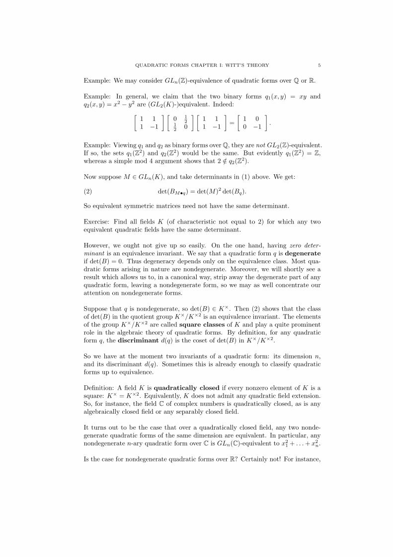
Example: In general, we claim that the two binary forms q1(x, y) = xy andq2(x, y) = x2 − y2 are (GL2(K)-)equivalent. Indeed:[

1 11 −1

] [0 1

212 0

] [1 11 −1

]=

[1 00 −1

].

Example: Viewing q1 and q2 as binary forms overQ, they are not GL2(Z)-equivalent.If so, the sets q1(Z2) and q2(Z2) would be the same. But evidently q1(Z2) = Z,whereas a simple mod 4 argument shows that 2 /∈ q2(Z2).

Now suppose M ∈ GLn(K), and take determinants in (1) above. We get:

(2) det(BM•q) = det(M)2 det(Bq).

So equivalent symmetric matrices need not have the same determinant.

Exercise: Find all fields K (of characteristic not equal to 2) for which any twoequivalent quadratic fields have the same determinant.

However, we ought not give up so easily. On the one hand, having zero deter-minant is an equivalence invariant. We say that a quadratic form q is degenerateif det(B) = 0. Thus degeneracy depends only on the equivalence class. Most qua-dratic forms arising in nature are nondegenerate. Moreover, we will shortly see aresult which allows us to, in a canonical way, strip away the degenerate part of anyquadratic form, leaving a nondegenerate form, so we may as well concentrate ourattention on nondegenerate forms.

Suppose that q is nondegenerate, so det(B) ∈ K×. Then (2) shows that the classof det(B) in the quotient group K×/K×2 is an equivalence invariant. The elementsof the group K×/K×2 are called square classes of K and play a quite prominentrole in the algebraic theory of quadratic forms. By definition, for any quadraticform q, the discriminant d(q) is the coset of det(B) in K×/K×2.

So we have at the moment two invariants of a quadratic form: its dimension n,and its discriminant d(q). Sometimes this is already enough to classify quadraticforms up to equivalence.

Definition: A field K is quadratically closed if every nonzero element of K is asquare: K× = K×2. Equivalently, K does not admit any quadratic field extension.So, for instance, the field C of complex numbers is quadratically closed, as is anyalgebraically closed field or any separably closed field.

It turns out to be the case that over a quadratically closed field, any two nonde-generate quadratic forms of the same dimension are equivalent. In particular, anynondegenerate n-ary quadratic form over C is GLn(C)-equivalent to x2

1 + . . .+ x2n.

Is the case for nondegenerate quadratic forms over R? Certainly not! For instance,

6 PETE L. CLARK

consider the following forms:

q1(x, y) = x2 + y2.

q2(x, y) = x2 − y2.

q3(x, y) = −x2 − y2.

I claim that no two of these forms are equivalent. Indeed, their correspondingquadratic functions have different images:

q1(R2) = [0,∞), q2(R2) = R, q3(R2) = (−∞, 0].

To explain carefully why this distinguishes the equivalence classes of forms, weintroduce another fundamental definition: if α ∈ K×, we say that a quadraticform q represents α iff α is in the image of the associated function, i.e., iff thereexists x ∈ Kn such that q(x) = α. But now suppose that q represents α and letM ∈ GLn(R). Choose x ∈ Kn such that q(x) = α. Then

(M · q)(M−1x) = q(MM−1x) = q(x) = α.

That is:

Proposition 2. Equivalent quadratic forms represent exactly the same set of scalars.

Following T.-Y. Lam, we define

D(q) = q(Kn) \ {0}to be the set of all nonzero values of K represented by q. Unlike the dimension orthe determinant, D(q) is a “second order” invariant, i.e., rather than being a singlenumber or field element, it is a set of field elements.

On the other hand, D(q) = D(q′) need not imply that q ∼= q′. Indeed, over Rthe two forms

(3) q1 = x21 − x2

2 + x23 + x2

4, q2 = x21 − x2

2 − x23 − x2

4

have the same dimension, the same discriminant, and both represent all real num-bers. The analyst’s proof of this is to observe that they clearly represent arbitrarilylarge positive and arbitrarily small negative values and apply the Intermediate Valuetheorem. The algebraist’s proof is that q1(x1, x2, 0, 0) = q2(x1, x2, 0, 0) = x2

1 − x22,

which by Example X.X above is equivalent toH(x, y) = xy, which visibly representsall elements of K×. But in fact they are not equivalent, as was first established bythe 19th century mathematician J.J. Sylvester. We will be able to establish this,and indeed to describe all isomorphism classes of quadratic forms over R, once wehave developed the basic theory of isotropic and hyperbolic subspaces.

Let q be an n-ary quadratic form over K. Then, with respect to the GLn(K)-action on the space of all n-ary quadratic forms, consider the isotropy subgroup

Oq = {M ∈ GLn(K) | M • q = q}.

Exercise: Let B be the symmetric matrix of the n-ary quadratic form q.a) Show that Oq = {M ∈ GLn(K) | MTBM = B}.b) Show that if q ∼ q′, then Oq is conjugate (in GLn(K)) to Oq′ . In particular, theisomorphism class of Oq is an equivalence invariant of q.c) Suppose q = x2

1+ . . .+x2n. Show that Oq is the standard orthogonal group O(n).

QUADRATIC FORMS CHAPTER I: WITT’S THEORY 7

d) For those who know the definition of linear algebraic groups, confirm that Oq

has the natural structure of a linear algebraic group. If q is nondegenerate, whatis the dimension of Oq?e) If K is a topological field, then Oq is a K-analytic Lie group. In case K = R,show that Oq is compact iff q is either positive or negative definite.f) Let q1 and q2 be the real quadratic forms of (3). Are their isotropy subgroupsisomorphic?

Similarities: Let Gm(K) = K× be the multiplicative group of K. Since Gm isthe center of GLn(K) – i.e., the scalar matrices – the above action of GLn(K) onQn restricts to an action of Gm. However, there is another action of Gm on Qn

which is relevant to the study of quadratic forms: namely α · q = αq, i.e., we scaleall of the coefficients of q by α ∈ Gm. If q′ = α ·q, we say that q and q′ are similar.

The two actions are related as follows:

α • q = α2 · q.

Since the • action of GLn(K) preserves equivalence of quadratic forms (by defini-tion), it follows that there is an induced action of K×/K×2 on the set of equivalenceclasses.

Exercise: Let q be an n-ary quadratic form. Let D(q) = {α ∈ Gm | α · q ∼ q}.a) Show that D(q) is a subgroup of Gm.b) Compute D(q) for the form x2

1 + . . .+ x2n over R.

c) Compute D(q) for the hyperbolic plane H = x2 − y2 over any field K.

3. The category of quadratic spaces

In the previous section we saw some advantages of the symmetric matrix approachto quadratic forms: it gave a very concrete and transparent perspective on theactions of GLn(K) and Gm on Qn. In this section we turn to the coordinate-freeapproach to quadratic forms, that of a finite-dimensional K-vector space V en-dowed with a symmetric bilinear form B : V × V → K. To be precise, we call sucha pair (V,B) a quadratic space.3

We pause to recall the meaning of nondegeneracy in the context of bilinear forms.Namely, let V be any K-vector space and B : V × V → K be any bilinear form.Then B induces a linear map LB from V to its dual space V ∨ = Hom(V,K),namely v 7→ B(v, ). We say that B is nondegenerate if LB is an isomorphism.In this purely algebraic context, this is only possible if V is finite-dimensional – ifV is an infinite-dimensional K-vector space, then dimV ∨ > dimV , so they are notisomorphic by any map, let alone by LB – in which case, since dimV = dimV ∨, itis equivalent to LB being injective. In other words, to test for the nondegeneracyof a bilinear form B, it suffices to show that if v ∈ V is every vector such thatB(v, w) = 0 for all w ∈ W , then necessarily v = 0.

3Probably it would be even more pedantically correct to call it a “symmetric bilinear space”,

but this is not the standard terminology. As we have seen, the data of B and the associatedquadratic function q are interchangeable in our present context.

8 PETE L. CLARK

In the case of quadratic forms we have now given two definitions of nondegen-eracy: one in terms of any associated symmetric matrix, and the other in terms ofthe associated symmetric bilinear form. So we had better check that they agree:

Proposition 3. The two notions of nondegeneracy coincide for quadratic forms:that is, a symmetric bilinear form B on a finite-dimensional vector space is non-degenerate iff its defining symmetric matrix (with respect to any basis of V ) hasnonzero determinant.

Proof. Choose a basis e1, . . . , en for V and define a matrix B with (i, j) entrybij = B(ei, ej). Then we have

B(v, w) = wTBv.

If the matrix B is singular, then there exists a nonzero v ∈ V such that Bv = 0,and then the above equation implies B(v, w) = 0 for all w ∈ W . Conversely, ifB is nonsingular, then for any nonzero v ∈ V , Bv is not the zero vector, so thereexists at least one i, 1 ≤ i ≤ n for which the ith component of Bv is nonzero. ThenB(v, ei) = 0. �

A map of quadratic spaces (V,BV ) → (W,BW ) is a K-linear map L : V → Wwhich “respects the bilinear form structure”: precisely:

∀v1, v2 ∈ V,BW (L(v1), L(v2)) = BV (v1, v2).

An isometric embedding is a morphism of quadratic spaces whose underlyinglinear map is injective.

Proposition 4. Let f : (V,Bv) → (W,BW ) be a map of quadratic spaces. If BV

is nondegenerate, then f is an isometric embedding.

Proof. Let v ∈ V be such that f(v) = 0. Then, for all v′ ∈ V , we have

0 = BW (0, f(v′)) = BW (f(v), f(v′)) = BV (v, v′).

Thus by the definition of nondegeneracy we must have v = 0. �

Exercise: Let ι : (V,BV ) → (W,BW ) be an isometric embedding of quadraticspaces. Show that the following are equivalent:(i) There exists an isometric embedding ι′ : (W,BW ) → (V,BV ) such that ι′◦ι = 1V ,ι ◦ ι′ = 1V ′ .(ii) ι is surjective.An isometric embedding satisfying these conditions will be called an isometry.

The category of quadratic spaces over K has as its objects the quadratic spaces(V,BV ) and morphisms isometric embeddings between quadratic spaces.

If (V,BV ) is a quadratic space and W ⊂ V is a K-subspace, let BW be the re-striction of BV to W .

Exercise: Show that (W,BW ) ↪→ (V,BV ) is an isometric embedding.

Does the category of quadratic spaces have an initial object? Yes, a zero-dimensionalvector space V = {0} with the unique (zero) map V ×V → K. Note that this bilin-ear form is nondegenerate according to the definition. (Presumably the determinant

QUADRATIC FORMS CHAPTER I: WITT’S THEORY 9

of a “0 × 0” matrix is 1, but we do not insist upon this.) This may seem like apointless convention, but it is not: it will be needed later to give the identity ele-ment of the Witt group of K.

Exercise: Show that the category of quadratic spaces over K has no final object.

The category of quadratic spaces admits finite direct sums. In other words, giventwo quadratic spaces V and W , there exists a quadratic space V ⊕W together withisometries V → V ⊕W , W → V ⊕W , such that every pair of isometries V → Z,W → Z factors uniquely through V ⊕W . Indeed, the underlying vector space onV ⊕W is the usual vector space direct sum, and the bilinear form is

BV⊕W ((v1, w1), (v2, w2)) := BV (v1, v2) +BW (w1, w2).

Fixing bases e1, . . . , em of V and e′1, . . . , e′n of W , if the symmetric matrices for the

BV and BW are B1 and B2, respectively, then the matrix for BV⊕W is the blockmatrix [

B1 00 B2

].

It is common to refer to the categorical direct sum of quadratic spaces as the or-thogonal direct sum. However, in our work, whenever we write down an externaldirect sum, we will always mean this “orthogonal” direct sum.

One can also define a tensor product of quadratic spaces (V,BV ) and (W,BW ).Again the underlying vector space is the usual tensor product V ⊗ W , and thebilinear form is given on basis elements as

BV⊗W (v1 ⊗ w1, v2 ⊗ w2) := BV (v1, v2) ·BW (w1, w2),

and extended by bilinearity. The associated symmetric matrix is the Kroneckerproduct. In particular, if with respect to some bases (ei), (e

′j) of V and W we

have diagonal matrices B1 = ∆(a1, . . . , am), B2 = ∆(b1, . . . , bn), then the matrixof BV⊗W is the diagonal mn×mn matrix ∆(aibj).

4. Orthogonality in quadratic spaces

Let (V,B) be a quadratic space, and let W1, W2 be subspaces. We say W1 andW2 are orthogonal subspaces if for all v1 ∈ W1, we have v2 ∈ W2, B(v1, v2) = 0.The notation for this is W1 ⊥ W2.

Exercise: Let (V1, B1), (V2, B2) be quadratic spaces. Identifying Vi with its iso-metric image in V1 ⊕ V2, show that V1 ⊥ V2. State and prove a converse result.

Let (V,B) be a quadratic space, andW ⊂ V a subspace. We define the orthogonalcomplement

W⊥ = {v ∈ V | ∀w ∈ W, B(v, w) = 0}.In other words, W⊥ is the maximal subspace of V which is orthogonal to W .

Exercise: Show that W 7→ W⊥ gives a self-dual Galois connection.

Example: If K = R, a quadratic space (V,B) is an inner product space if

10 PETE L. CLARK

B is positive definite: B(v, v) ≥ 0 for all v ∈ V and B(v, v) = 0 =⇒ v = 0. Inthis special case the notions of orthogonal direct sum, orthogonal complement (andorthogonal basis!) are familiar from linear algebra.

However, in general a quadratic space may have nonzero vectors v for whichB(v, v) =0, and this lends the theory a different flavor.

Definition: Let (V,B) be a nondegenerate quadratic space. A vector v ∈ V issaid to be isotropic if q(v) = B(v, v) = 0 and anisotropic otherwise. V itselfis said to be isotropic if there exists a nonzero isotropic vector and otherwiseanistropic. Thus an inner product space is (in particular) an anisotropic real qua-dratic space.

Definition: The radical of V is rad(V ) = V ⊥.

Exercise: Show that a quadratic space (V,B) is nondegenerate iff rad(V ) = 0.

Exercise: Show that rad(V ⊕W ) = rad(V )⊕ rad(W ).

Proposition 5. (Radical Splitting) Let (V,B) be any quadratic space. Then thereexists a nondegenerate subspace W such that

V = rad(V )⊕W

is an internal orthogonal direct sum decomposition.

Proof. Since by definition rad(V ) is orthogonal to all of V , any complementarysubspace W to rad(V ) in the sense of usual linear algebra will give rise to anorthogonal direct sum decomposition V = rad(V )⊕W . It follows from the precedingexercise that W is nondegenerate. �Remark: The complementary subspace W is in general far from being unique.

Remark: It is of interest to have an algorithmic version of this result. This will fol-low immediately from the algorithmic description of the diagonalization proceduregiven following Theoerem 9.

Proposition 6. Let (V,B) be a quadratic space, and W ⊂K V a nondegeneratesubspace. Then V = W ⊕W⊥.

Proof. By Exercise X.X, since W is nondegenerate, rad(W ) = W ∩W⊥ = 0, so itmakes sense to speak of the subspace W ⊕W⊥ of V . Now let z ∈ V , and considerthe associated linear form Z ∈ Hom(W,K) given by Z(v) := B(z, v). Since W isnondegenerate, there exists w ∈ W such that for all v ∈ W ,

Z(v) = B(z, v) = B(w, v).

Thus w′ = z − w ∈ W⊥ and z = w + w′. �Proposition 7. Let (V,B) be a nondegenerate quadratic space and W ⊂ V anarbitrary subspace. Then we have:

(4) dimW + dimW⊥ = dimV.

(5) (W⊥)⊥ = W.

QUADRATIC FORMS CHAPTER I: WITT’S THEORY 11

Proof. a) Consider the linear map L : V → W∨ given by v 7→ (w 7→ B(v, w)).Evidently Ker(L) = W⊥. Moreover, this map factors as the composite V → V ∨ →W∨, where the first map is surjective by nondegeneracy and the second map isevidently surjective (any linear form on a subspace extends to a linear form on thewhole space). Therefore L is surjective, so we get

dimV = dimW⊥ + dimW∨ = dimW⊥ + dimW.

b) The inclusion W ⊂ (W⊥)⊥ is a tautology which does not require the non-degeneracy of V : indeed every vector in W is orthogonal to every vector whichis orthogonal to every vector in W ! On the other hand, by part a) we havedimW⊥ + dim(W⊥)⊥ = dimV , so dimW = dim(W⊥)⊥. Since W is finite-dimensional, we conclude W = (W⊥)⊥. �

Corollary 8. For a nondegenerate quadratic space (V,B) and W ⊂K V , TFAE:(i) W ∩W⊥ = 0.(ii) W is nondegenerate.(iii) W⊥ is nondegenerate.

Exercise X.X: Prove Corollary 8.

5. Diagonalizability of Quadratic Forms

Let q ∈ Qn be an n-ary quadratic form. We say that q is diagonal if either of thefollowing equivalent conditions are satisfied:

(D1) Its defining quadratic polynomial is of the form∑

i aix2i .

(D2) Its defining symmetric matrix is diagonal.

Exercise: Show that a diagonal form is nondegenerate iff ai = 0 for all i.

Exercise: a) Let σ ∈ Sn be a permutation, and let Mσ be the matrix obtained byapplying the permutation σ to the columns of the n×n identity matrix. Show thatif D = ∆(a1, . . . , an) is any diagonal matrix, then MT

σ DM = ∆(aσ(1), . . . , aσ(n)).In particular, reordering the diagonal entries of a diagonal quadratic form does notchange its equivalence class.b) For α ∈ K×, find an explicit matrix M such that

MT∆(a1, . . . , an)M = ∆(α2a1, . . . , an).

c) Show that any two nondegenerate diagonal quadratic forms over a quadraticallyclosed field are equivalent.d) Use the spectral theorem from linear algebra to show that any real quadraticform is equivalent to a diagonal form. Deduce that any nondegenerate real qua-dratic form is equivalent to ∆(1, . . . , 1,−1, . . . ,−1) where there are 0 ≤ r instancesof 1 and 0 ≤ s instances of −1, with r + s = n.

In general, let us say that an quadratic form q ∈ Qn(K) is diagonalizable ifit is GLn(K)-equivalent to a diagonal quadratic form. (By convention, we decreethe trivial quadratic form to be diagonalizable.) We can now state and prove oneof the most basic results of the theory.

Theorem 9. Every quadratic form over K is diagonalizable.

12 PETE L. CLARK

Before giving the proof, let us state the result in two equivalent forms, both usingthe language of quadratic spaces. A diagonalizable quadratic space (V,B) is onefor which there exist one-dimensional subspaces W1, . . . ,Wn such that

V = W1 ⊕ . . .⊕Wn.

Equivalently, there exists an orthogonal basis (e1, . . . , en) for V , i.e., one forwhich B(ei, ej) = 0 for all i = j.

Proof. We go by induction on the dimension of V , the case n = 0 being trivial.Suppose the result is true for all quadratic spaces over K of dimension less thann, and let (V,B) be an n-dimensional quadratic space. If B is identically zero,the result is obvious, so let us assume not. If the asociated quadratic form q(x) =B(x, x) were identically zero, then by the polarization identity, so would B be.Thus we may assume that there exists v1 ∈ V with q(v1) = 0. Then W1 = ⟨v1⟩ isnondegenerate, and by Proposition 6 we have V = W1 ⊕W⊥

1 . We are finished byinduction! �

This theorem and proof can be restated in the language of symmetric matrices.Namely, let B be an n× n symmetric matrix with coefficients in K. Then by per-forming a sequence of simultaneous row-and-column operations on B – equivalently,multiplying on the right by an elementary matrix E and on the left by its transpose– we can bring B to diagonal form.

Here is an algorithm description: if B = 0, we’re done. Otherwise, there exists anonzero entry bij . By taking E to be the elementary matrix corresponding to thetransposition (1i), we get a nonzero entry α = b′j1. If j = 1, great. If not, thenby adding the jth row to the first row – and hence also the jth column to the firstcolumn – we get a matrix B′′ with b′′11 = 2α (which is nonzero since K does nothave characteristic 2!). Then, since every element of K is a multiple of 2α, by usualrow (+ column) reduction we can get an congruent matrix B′′′ with b′′′1j = 0 for allj > 1. In the above proof, this corresponds to finding an anisotropic vector andsplitting off its orthogonal complement. Now we proceed by induction.

Remark: As alluded to above, Theorem 9 is direct generalization of Proposition5 (Radical Splitting), and the algorithmic description given above in particulargives an effective procedure that Proposition.

Corollary 10. Let V be a nondegenerate quadratic space.a) For any anisotropic vector v, there exists an orthogonal basis (v, e2, . . . , en).b) If α ∈ K× is represented by q, then (V, q) ∼= αx2

1 + α2x22 + . . .+ αnx

2n.

Proof. Part a) is immediate from the proof of Theorem 9, and part b) followsimmediately from part a). �

Corollary 11. Let q be a nondegenerate binary form of discriminant d whichrepresents α ∈ K×. Then q ∼= ⟨α, αd⟩. In particular, two nondegenerate binaryforms are isometric iff they have the same discriminant and both represent any oneelement of K×.

Proof. By Corollary 10, q ∼= αx21 + α2x

22. The discriminant of q is on the one hand

d (mod K)×2 and on the other hand αα2 (mod K)×2 so there exists a ∈ K× such

QUADRATIC FORMS CHAPTER I: WITT’S THEORY 13

that αα2 = da−2. So

q ∼= αx21 +

(d

αa2

)x22 = αx2

1 + αd( x2

αa

)2 ∼= αx21 + αdx2

2.

�

Exercise: Show that the usual Gram-Schmidt process from linear algebra works toconvert any basis to an orthogonal basis, provided we have q(x) = 0 for all x = 0.

In view of Theorem 9 it will be useful to introduce some streamlined notation fordiagonal quadratic forms. For any α ∈ K, we let ⟨α⟩ denote the one-dimensionalquadratic space equipped with a basis vector e with q(e) = α. For α1, . . . , αn, wewrite ⟨a1, . . . , an⟩ for

⊕ni=1⟨ai⟩, or in other words, for the quadratic form corre-

sponding to the matrix ∆(a1, . . . , an).

Exercise: Convert this proof into an algorithm for diagonalizing quadratic forms.(Hint: explain how to diagonalize a corresponding symmetric matrix using simul-taneous row and column operations.)

Remark: The result of Theorem 9 does not hold for fields of characteristic 2.For instance, the binary quadratic form q(x, y) = x2 + xy + y2 over F2 is notGL2(F2)-equivalent to a diagonal form. One way to see this is to observe thatq is anisotropic over F2, whereas any diagonal binary form is isotropic: certainlyax2+ by2 is isotropic if ab = 0; and otherwise ax2+ by2 = (x+ y)2 and an isotropicvector is (x, y) = (1, 1).

6. Isotropic and hyperbolic spaces

Recall that a quadratic space V is isotropic if it is nondegenerate and there existsa nonzero vector v such that q(v) = 0.

The basic example of an isotropic space is the hyperbolic plane, given by H(x, y) =xy, or in equivalent diagonal form as H(x, y) = 1

2x2 − 1

2y2. A quadratic space is

hyperbolic if it is isometric to a direct sum of hyperbolic planes.

A subspace W of a quadratic space (V,B) is totally isotropic if B|W ≡ 0.4

We come now to what is perhaps the first surprising result in the structure theoryof nondegenerate quadratic forms. It says that, in some sense, the hyperbolic planeis the only example of an isotropic quadratic space. More precisely:

Theorem 12. Let (V,B) be an isotropic quadratic space. Then there is an isomet-ric embedding of the hyperbolic plane into (V,B).

Proof. Since B is nondegenerate, there exists w ∈ V with B(u1, w) = 0. By suitablyrescaling w, we may assume that B(u1, w) = 1. We claim that there exists a unique

4We have some misgivings here: if 0 = W ⊂ V is a totally isotropic subspace, then viewed asa quadratic space in its own right, W is not isotropic, because isotropic subspaces are required

to be nondegenerate. Nevertheless this is the standard terminology and we will not attempt tochange it.

14 PETE L. CLARK

α ∈ K such that q(αu1 + w) = 0. Indeed,

q(αu1 + w) = α2q(u1) + 2αB(u1, w) + q(w) = 2α+ q(w),

so we may take α = −q(w)2 . Putting u2 = αu1 + w, we have q(u1) = q(u2) = 0 and

B(u1, u2) = B(u1, αu1 + w) = αq(u1) +B(u1, w) = 1,

so that the quadratic form q restricted to the span of u1 and u2 is, with respect tothe basis u1, u2, the hyerbolic plane: q(xu1 + yu2) = xy. �Here is a generalization.

Theorem 13. Let (V,B) be a nondegenerate quadratic space and U ⊂ V a totallyisotropic subspace with basis u1, . . . , um. Then there exists a totally isotropic sub-space U ′, disjoint from U , with basis u′

1, . . . , u′m such that B(ui, u

′j) = δ(i, j). In

particular ⟨U,U ′⟩ ∼=⊕m

i=1 H.

Proof. We proceed by induction on m, the case m = 1 being Theorem 12. SinceB is nondegenerate, there exists w ∈ V with B(u1, w) = 0. By suitably rescalingw, we may assume that B(u1, w) = 1. We claim that there exists a unique α ∈ Ksuch that q(αu1 + w) = 0. Indeed,

q(αu1 + w) = α2q(u1) + 2αB(u1, w) + q(w) = 2α+ q(w),

so we may take α = −q(w)2 . Putting u2 = αu1 + w, we have q(u1) = q(u2) = 0 and

B(u1, u2) = B(u1, αu1 + w) = αq(u1) +B(u1, w) = 1,

so that the quadratic form q restricted to the span of u1 and u2 is, with respect tothe basis u1, u2, the hyerbolic plane: q(xu1 + yu2) = xy.

Now assume the result is true for all totally isotropic subspaces of dimensionsmaller thanm. LetW = ⟨u2, . . . , um⟩. If we hadW⊥ ⊆ ⟨u1⟩⊥, then taking “perps”and applying Proposition 7 we would get ⟨u1⟩ ⊂ W , a contradiction. So there existsv ∈ W⊥ such that B(u1, v) = 0. As above, the subspace H1 spanned by u1 andv is a hyperbolic plane and hence contains a vector u′

1 such that B(u′1, u

′1) = 0,

B(u1, u′1) = 1. By construction we have H1 ⊂ W⊥; taking perps gives W ⊂ H⊥

1 .Since H⊥

1 is again a nondegenerate quadratic space, we may apply the inductionhypothesis to W to find a disjoint totally isotropic subspace W ′ = ⟨u′

2, . . . , u′n⟩ with

each ⟨ui, ui⟩ a hyperbolic plane. �The following is an immediate consequence.

Corollary 14. Let W be a maximal totally isotropic subspace of a nondegeneratequadratic space V . Then dimW ≤ 1

2 dimV . Equality holds iff V is hyperbolic.

It will convenient to have a name for the subspace U ′ shown to exist under the hy-potheses of Theorem 13, but there does not seem to be any standard terminology.So, to coin a phrase, we will call U ′ an isotropic supplement of U .

We define a quadratic form q to be universal if it represents every element ofK×. Evidently the hyperbolic plane H = xy is universal: take x = α, y = 1.

Corollary 15. Any isotropic quadratic space is universal.

Proof. This follows immediately from Theorem 12. �Exercise X.X: Give an example of an anisotropic universal quadratic form.

QUADRATIC FORMS CHAPTER I: WITT’S THEORY 15

Corollary 16. For any α ∈ K×, the rescaling α ·H is isomorphic to H.

Proof. α ·H is a two-dimensional isotropic quadratic space. Apply Theorem 12. �

Corollary 17. Any quadratic space V admits an internal orthogonal direct sumdecomposition

V ∼= rad(V )⊕n⊕

i=1

H⊕ V ′,

where n ∈ N and V ′ is anisotropic.

Proof. By Proposition 5 we may assume V is nondegenerate. If V is anisotropic,we are done (n = 0). If V is isotropic, then by Theorem 12 there is a hyperbolicsubspace H ⊂ V . Since H is nondegenerate, by Proposition 6 V = H ⊕ H⊥, withH⊥ nondegenerate of smaller dimension. We are finished by induction. �

Remark: This is half (the easier half) of the Witt Decomposition Theorem.The other, deeper, half is a uniqueness result: the number n and the isometry classof V ′ are independent of the choice of direct sum decomposition.

Theorem 18. (First Representation Theorem) Let q be a nondegenerate quadraticform, and let α ∈ K×. TFAE:(i) q represents α.(ii) q ⊕ ⟨−α⟩ is isotropic.

Proof. If q represents α, then by Remark X.X, q is equivalent to a form ⟨α, α2, . . . , αn⟩.Then q ⊕ ⟨−α⟩ contains (an isometric copy of) ⟨α,−α⟩ = α ·H ∼= H so is isotropic.Conversely, we may assume q = ⟨α1, . . . , αn⟩, and our assumption is that thereexist x0, . . . , xn, not all 0, such that

−αx20 + α1x

21 + . . .+ αnx

2n = 0.

There are two cases. If x0 = 0, then α1(x1/x0)2 + . . . + αn(xn/x0)

2 = α, so qrepresents α. If x0 = 0, then x = (x1, . . . , xn) is a nonzero isotropic vector for q, soq is isotropic and thus represents every element of K×, including α. �

This has the following easy consequence, the proof of which is left to the reader.

Corollary 19. For a field K and n ∈ Z+, TFAE:(i) Every nondegenerate n-ary quadratic form over K is universal.(ii) Every nondegenerate (n+ 1)-ary quadratic form over K is isotropic.

Lemma 20. (Isotropy Criterion) Let m,n ∈ Z+, let f(x1, . . . , xm) and g(y1, . . . , yn)be nondegenerate quadratic forms, and put h = f − g. TFAE:(i) There is α ∈ K× which is represented by both f and g.(ii) The quadratic form h is isotropic.

Proof. (i) =⇒ (ii): Suppose there are x ∈ Km, y ∈ Kn such that f(x) = g(y) = α.Then h(x, y) = α−α = 0 and since f(x) = α = 0, some coordinate of x is nonzero.(ii) =⇒ (i): Let (x, y) ∈ Km+n \ {(0, . . . , 0)} be such that h(x, y) = f(x) −g(y) = 0. Let α be the common value of f(x) and f(y). If α = 0, we’re done.Otherwise at least one of f and g is isotropic: say it is f . Then f contains H andtherefore represents every element of K×, so in particular represents g(e1) = 0,where e1, . . . , en is an orthogonal basis for Kn. �

16 PETE L. CLARK

7. Witt’s theorems: statements and consequences

In this section we state the fundamental result of Witt on which the entire algebraictheory of quadratic forms is based. It turns out that there are two equivalentstatements of Witt’s result: as an extension theorem and as a cancellationtheorem. We now state these two theorems, demonstrate their equivalence, andderive some important consequences. The proof of the Witt Cancellation Theoremis deferred to the next section.

Theorem 21. (Witt Cancellation Theorem) Let U1, U2, V1, V2 be quadratic spaces,with V1 and V2 isometric. If U1 ⊕ V1

∼= U2 ⊕ V2, then U1∼= U2.

Theorem 22. (Witt Extension Theorem) Let X1 and X2 be isometric quadraticspaces. Suppose we are given orthogonal direct sum decompositions X1 = U1 ⊕ V1,X2 = U2 ⊕ V2 and an isometry f : V1 → V2. Then there exists an isometryF : X1 → X2 such that F |V1 = f and F (U1) = U2.

Let us demonstrate the equivalence of Theorems 22 and 21. Assume Theorem 22,and let U1, U2, V1, V2 be as in Theorem 21. Put X1 = U1 ⊕ V1, X2 = U2 ⊕ V2, andlet f : V1 → V2 be an isometry. By Theorem 22, U1 and U2 are isometric.

Conversely, assume Theorem 21, and let X1, X2, U1, U2, V1, V2 be as in Theorem22. Then Witt Cancellation implies that U1

∼= U2, say by an isometry fU : U1 → U2.Then F = fU ⊕ f : X1 → X2 satisfies the conclusion of Theorem 22.

Remark: The statement of Theorem 22 is taken from [Cop, Prop. VII.18]. Theadvantage has just been seen: its equivalence with the Witt Cancellation Theorem(in the most general possible form) is virtually immediate. Each of the followingresults, which contain further assumptions on nondegeneracy, is sometimes referredto in the literature as “Witt’s Isometry Extension Theorem”.

Corollary 23. Let X be a quadratic space and V1, V2 ⊂ X be nondegenerate sub-spaces. Then any isometry f : V1 → V2 extends to an isometry F of X.

Proof. Put U1 = V ⊥1 , U2 = V ⊥

2 . Because of the assumed nondegeneracy of V1 andV2, we have X = U1 ⊕ V1 = U2 ⊕ V2. Theorem 22 now applies with X = X1 = X2

to give an isometry F of X extending f . �Remark: The conclusion of Corollary 23 may appear weaker than that of Theorem22, but this is not so. Since V1 and V2 are nondegenerate, any extended isometryF must map U1 to U2: since f(V1) = V2, f(U1) = f(V ⊥

1 ) = f(V1)⊥ = V ⊥

2 = U2.

Corollary 24. Let X be a nondegenerate quadratic space and Y1 ⊂ X any subspace.Then any isometric embedding f : Y1 → X is an extends to an isometry F of X.

Proof. Put Y2 = f(Y1). Note that if Y1 is nondegenerate, then so is Y2 and we mayapply Corollary 23. Our strategy of proof is to reduce to this case. Using Proposi-tion 5 we may write Y1 = U1⊕W1 with U1 totally isotropic and W1 nondegenerate.Evidently U1 ⊂ W⊥

1 ; since X and W1 are nondegenerate, by Corollary 8 W⊥1 is

nondegenerate as well. We may therefore apply Theorem 13 to find an isotropicsupplement U ′

1 to U1 inside W⊥1 . Let V1 = ⟨U1, U

′1⟩⊕W1. Then V1 is nondegenerate

and the natural inclusion Y1 ↪→ V1 is, of course, an isometric embedding. We mayapply the same reasoning to Y2

∼= U2 ⊕ W2 to get an isotropic supplement U ′2 to

U2 inside W⊥2 and Y2 ↪→ V2 = ⟨U2, U

′2⟩ ⊕ W2. Since Ui = rad(Yi) and Y1 and Y2

QUADRATIC FORMS CHAPTER I: WITT’S THEORY 17

are isometric, U1∼= U2, and then ⟨U1, U

′1⟩ and ⟨U2, U

′2⟩ are hyperbolic spaces of the

same dimension, hence isometric. By Witt Cancellation, W1∼= W2. It follows that

V1 and V2 are isometric, and we finish by applying Corollary 23. �

This has the following interesting consequence.

Theorem 25. Let V be a nondegenerate quadratic space. Then, for any 0 ≤ d ≤12 dimV , the group of isometries of V acts transitively on the set of all totallyisotropic subspaces of dimension d.

Exercise: Let X be the quadratic space ⟨1,−1, 0⟩. Let V1 = ⟨e1+e2⟩ and V2 = ⟨e3⟩.a) Show that there exists an isometry f : V1 → V2.b) Show that f does not extend to an isometry of X.

Corollary 23 is equivalent to a weak version of Witt Cancellation in which wemake the additional hypothesis that V1 (hence also V2) is nondegenerate. The oneapplication of being able to cancel also degenerate subspaces is the following result.

Theorem 26. (Witt Decomposition Theorem) Let (V,B) be a quadratic space.Then there exists an orthogonal direct sum decomposition

V ∼= rad(V )⊕I⊕

i=1

H⊕ V ′,

where V ′ is an anistropic quadratic space. Moreover the number I = I(V ) and theisometry class of V ′ are independent of the choice of decomposition.

Proof. The existence of such a decomposition has already been shown: Corollary17. The uniqueness follows immediately from the Witt Cancellation Theorem andthe fact that any isotropic quadratic form contains an isometrically embedded copyof the hyperbolic plane (Theorem 12). �

Remark: Theorem 26 is a good excuse for restricting attention to nondegeneratequadratic forms. Indeed, unless indication is expressly given to the contrary, wewill henceforth consider only nondegenerate quadratic forms.

Thus, assuming that V is nondegenerate, the natural number I(V ) is called theWitt index of V . By Exercise X.X, it can be characterized as the dimension ofany maximal totally isotropic subspace of V .

Theorem 27. (Sylvester’s Law of Nullity)Let n ∈ Z+ and r, s ∈ N with r + s = n. Define

qr,s = [r]⟨1⟩ ⊕ [s]⟨−1⟩,i.e., the nondegenerate diagonal form with r 1’s and s −1’s along the diagonal.Then any n-ary quadratic form over R is isomorphic to exactly one form qr,s.

Exercise: Use the Witt Decomposition Theorem to prove Theorem 27.

7.1. The Chain Equivalence Theorem.

In this section we present yet another fundamental theorem due E. Witt, albeitone of a more technical nature. This theorem will be needed at a key juncturelater on in the notes, namely in order to show that the Hasse-Witt invariant is

18 PETE L. CLARK

well-defined. The reader should feel free to defer reading about the proof, and eventhe statement, of the result until then.

Let q1 = ⟨a1, . . . , an⟩, q2 = ⟨b1, . . . , bn⟩ be two diagonal n-ary quadratic formsover K. We say that q1 and q2 are simply equivalent if there exist not neces-sarily distinct indices i and j such that ⟨ai, aj⟩ ∼= ⟨bi, bj⟩ and for all k = i, j, ak = bk.

The following exercises are very easy and are just here to keep the reader awake.

Exercise X.X: If q and q′ are simply equivalent, then they are isometric.

Exercise X.X: If n ≤ 2, then two n-ary quadratic forms q and q′ are simply equiv-alent iff they are isometric.

Exercise: If q and q′ are chain equivalent, then so are q ⊕ q′′ and q′ ⊕ q′′.

Despite the name, simple equivalence is not an equivalence relation: it is (obviously)reflexive and symmetric, but it is not transitive. For instance, let a ∈ K \ {0,±1}and n ≥ 3, then the forms q = ⟨1, . . . , 1⟩ and q′ = ⟨a2, . . . , a2⟩ are not simply equiv-alent, since at least three of their diagonal coefficients differ. However, if we putq1 = ⟨a2, a2, 1 . . . , 1⟩ q2 = ⟨a2, a2, a2, a2, 1, . . . 1⟩ and so forth, changing at each steptwo more of the coefficients of q to a2: if n is odd, then at the (final) n+1

2 th step, wechange the nth coefficient only. Then q is simply equivalent to q1 which is simplyequivalent to q2 . . . which is simply equivalent to qn which is simply equivalent to q′.

Let us temporarily denote the relation of simple equivalence by ∼. Since it isnot transitive, it is natural to consider its transitive closure, say ≈. As for anytransitive closure, we have q ≈ q′ iff there exists a finite sequence q0, . . . , qn+1 withq0 = q, qn+1 = q′ and qi ∼ qi+1 for all i. The reader may also verify that the tran-sitive closure of any reflexive, symmetric relation remains reflexive and symmetricand is thus an equivalence relation. In this case, we say that two quadratic formsq and q′ are chain equivalent if q ≈ q′.

Note that in our above example of two chain equivalent but not simply equiv-alent quadratic forms, q and q′ are in fact isometric. Indeed this must be true ingeneral since the relation of simple equivalence is contained in that of the equiva-lence relation of isometry, so therefore the equivalence relation generated by simpleequivalence must be contained in the equivalence relation of isometry. (Or just stopand think about it for a second: perhaps this explanation is more heavy-handedthan necessary.) So a natural question5 is how does chain equivalence compare toisometry. Is it possible for two isometric quadratic forms not to be chain equivalent?

Theorem 28. (Witt’s Chain Equivalence Theorem) For two n-ary quadratic formsq = ⟨α1, . . . , αn⟩, q′ = ⟨β1, . . . , βn⟩, TFAE:(i) q ≈ q′ (q and q′ are chain equivalent).(ii) q ∼= q′ (q and q′ are isometric).

Proof. The implication (i) =⇒ (ii) has been established above. It remains to showthat (ii) =⇒ (i).

5Well, as natural as the relation of simple equivalence, anyway.

QUADRATIC FORMS CHAPTER I: WITT’S THEORY 19

Step 0: Using Proposition 5 (Radical Splitting), we easily reduce to the case inwhich q and q′ are nondegenerate, i.e., αi, βj ∈ K× for all i, j. (Moreover this willbe the case of interest to us in the sequel.)Step 1: Because the symmetric group Sn is generated by transpositions, it followsthat for any permutation σ of {1, . . . , n} and any α1, . . . , αn ∈ K×, the (isometric!)quadratic forms ⟨α1, . . . , αn⟩ and ⟨ασ(1), . . . , ασ(n)⟩ are chain equivalent.Step 2: We prove that any two isometric nondegenerate n-ary quadratic forms qand q′ are chain equivalent, by induction on n. The cases n = 1, 2 have already beendiscussed, so assume n ≥ 3. Any form which is chain equivalent to q is isometricto q′ and hence represents β1. Among all n-ary forms ⟨γ1, . . . , γn⟩ which are chainequivalent to q, choose one such that

(6) β1 = γ1a21 + . . .+ γℓa

2ℓ

with minimal ℓ. We claim that ℓ = 1. Suppose for the moment that this is thecase. Then α is chain equivalent to a form ⟨β1a

−21 , γ2, . . . , γn⟩ and hence to a form

q1 = ⟨β1, γ2, . . . , γn⟩. Then, by Witt Cancellation, the form ⟨γ2, . . . , γn⟩ is isometricto ⟨β2, . . . , βn⟩, and by induction these latter two forms are chain equivalent. ByExercise X.X, the forms q1 and q′ are chain equivalent, hence q and q′ are chainequivalent.Step 4: We verify our claim that ℓ = 1. Seeking a contradiction we suppose thatℓ ≥ 2. Then no subsum in (6) can be equal to zero. In particular d := γ1a

21+γ2a

22 =

0, hence by Corollary 11 we have ⟨γ1, γ2⟩ ∼= ⟨d, γ1γ2d⟩. Using this and Step 1,

q ≈ ⟨γ1, . . . , γn⟩ ≈ ⟨d, γ1γ2d, γ3, . . . , γn⟩ ∼= ⟨d, γ3, . . . , γn, γ1γ2d⟩.But β1 = d+ γ3a

23 + . . .+ γℓa

2ℓ , contradicting the minimality of ℓ. �

8. Orthogonal groups, reflections and the proof of WittCancellation

8.1. The orthogonal group of a quadratic space.

Let V be a quadratic space. Then the orthogonal group O(V ) is, by definition,the group of all isometries from V to V , i.e., the group of linear automorphisms Mof V such that for all v, w ∈ V , B(v, w) = B(Mv,Mw). Identifying V with Kn

(i.e., choosing a basis) and B with the symmetric matrix (B(ei, ej)), the definitionbecomes

O(V ) = {M ∈ GLn(K) | ∀v, w ∈ Kn, vTBw = vTMTBMw}= {M ∈ GLn(K) | M • q = q}

where q is the associated quadratic form. In other words, O(V ) is none other thanthe isotropy group Oq of q for the GLn(K)-action on n-ary quadratic forms.

Remark: It is tempting to try to provide a conceptual explanation for the some-what curious coincidence of isotropy groups and automorphism groups. But thiswould involve a digression on the groupoid associated to a G-set, a bit of abstractnonsense which we will spare the reader...for now.

Although we introduced isotropy groups in §1.2 and remarked that the isotropygroup of the form [n]⟨1⟩ is the standard orthogonal group O(n), we did not providemuch information about orthogonal groups over an arbitrary field. Essentially all

20 PETE L. CLARK

we know so far is that equivalent forms have conjugate (in particular isomorphic)orthogonal groups. Here is one further observation, familiar from linear algebra.

By definition, for all M ∈ O(V ) we have MTBM = B; taking determinantsgives det(M)2 detB = detB. If (V,B) is nondegenerate, then detB = 0, and weconclude that detM = ±1. This brings us to:

Proposition 29. Let V be a nondegenerate quadratic space. We have a short exactsequence of groups

1 → O+(V ) → O(V )det→ {±1} → 1.

Proof. In other words, O+(V ) is by definition the subgroup of matrices in O(V )of determinant 1. It remains to see that there are also elements in O(V ) withdeterminant −1. However, we may assume that V is given by a diagonal matrix,and then M = ∆(1, . . . , 1,−1) is such an element. �

Exercise: Show that if V is degenerate, O(V ) contains matrices with determinantother than ±1.

Definition: We write O−(V ) for the elements of O(V ) of determinant −1. Ofcourse this is not a subgroup, but rather the unique nontrivial coset of O+(V ).

8.2. Reflection through an anisotropic vector.

We now introduce a fundamental construction which will turn out to generalizethe seemingly trivial observation that if q is diagonal, ∆(1, . . . , 1,−1) is an explicitelement in O−(V ). Indeed, let (V,B, q) be any quadratic space, and let v ∈ V bean anisotropic vector. We define an element τv ∈ O−(V ) as follows:

τv : x 7→ x− 2B(x, v)

q(v)v.

Note that in the special case in which V = Rn and B is positive definite, τv isreflection through the hyperplane orthogonal to v. In the general case we call τv ahyperplane reflection. We justify this as follows:

Step 1: τv is a linear endomorphism of V . (An easy verification.)

Step 2: Put W = ⟨v⟩⊥, so that V = W ⊕ ⟨v⟩. Let e1, . . . , en−1 be an orthogo-nal basis for W , so that (e1, . . . , en−1, v) is an orthogonal basis for V . Then, withrespect to this basis, the matrix representation of τv is indeed ∆(1, . . . , 1,−1). Itfollows that τv is an isometry, τ2v = 1V and det(τv) = −1.

Exercise: Let σ ∈ O(V ) and v ∈ V an anisotropic vector. Show that στvσ−1 = τσv.

Proposition 30. Let (V,B, q) be any quadratic space. Suppose that x, y ∈ Vare anisotropic vectors with q(x) = q(y). Then there exists τ ∈ O(V ) such thatτ(x) = y.

Proof. We compute

q(x+y)+q(x−y) = B(x+y, x+y)+B(x−y, x−y) = 2q(x)+2q(−y) = 4q(x) = 0.

QUADRATIC FORMS CHAPTER I: WITT’S THEORY 21

Therefore q(x + y) and q(x − y) are not both zero. Let us first suppose thatq(x− y) = 0. Then

q(x− y) = B(x, x) +B(y, y)− 2B(x, y) = 2B(x, x)− 2B(x, y) = 2B(x, x− y),

so that

τx−y x = x− 2B(x, x− y)

q(x− y)(x− y) = y,

hence τx−y is an isometry carrying x to y. Otherwise we have 0 = q(x + y) =q(x− (−y)), and the above argument shows that τx+yx = τx−(−y)x = −y and thus−(τx+yx) = y. �

8.3. Proof of Witt Cancellation.

We can now give the proof of the Witt Cancellation Theorem. First a slight sim-plification: if U1, U2, V1, V2 are quadratic spaces such that V1

∼= V2 and U1 ⊕ V1∼=

U2 ⊕ V2, then we have U2 ⊕ V2∼= U2 ⊕ V1, hence U1 ⊕ V1

∼= U2 ⊕ V1. So we mayassume: V1 = V2 = V , U1 ⊕ V ∼= U2 ⊕ V . We wish to conclude that U1

∼= U2.

Step 1: V is totally isotropic, say of dimension r and U1 is nondegenerate, sayof dimension s. Choose bases, and let B1 (resp. B2) be the symmetric matrix as-sociated to U1 (resp. U2), so that we are assuming the existence of M ∈ GLr+s(K)such that

MT

[0r 0r,s0s,r B2

]M =

[0r 0r,s0s,r B1

].

But writing M as a block matrix

[A BC D

], we find that the s × s submatrix in

the lower right hand corner of the left hand side is DTM2D. Thus M1 = DTM2D.Since M1 is nonsingular, so is D, and we conclude that U1

∼= U2.

Step 2: V is totally isotropic. Choose orthogonal bases for U1 and U2, and supposeWLOG that the matrix for U1 has exactly r zeros along the diagonal, whereas thematrix for U2 has at least r zeros. Then we can replace V by V ⊕ [r]⟨0⟩ and assumethat U1 is nondegenerate, reducing to Case 1.

Step 3: dimV = 1, say V = ⟨a⟩. If a = 0 we are done by Case 2, so we mayassume a = 0. Explicitly, choose a basis x, e2, . . . , en for W1 = ⟨a⟩ ⊕ U1 withq(x) = a and a basis (x′, e′2 . . . , e

′n) for W2 = ⟨a⟩ ⊕ U2 with q(x′) = a, and let

F : W1 → W2 be an isometry. Put y = F−1(x′) and U ′1 = F−1(U2), so that

W1 = ⟨x⟩ ⊕ U1 = ⟨y⟩ ⊕ U ′1.

By Proposition 30, there exists τ ∈ O(W1) such that τ(x) = y. Because ⟨x⟩ and⟨y⟩ are nondegenerate, we have U1 = ⟨x⟩⊥ and U ′

1 = ⟨y⟩⊥, so that (as in RemarkX.X above) we necessarily have τ(U1) = U ′

1. Thus U1∼= U ′

1∼= U2.

Step 4: General case: Write V = ⟨a1, . . . , an⟩. By Step 3 we can cancel ⟨a1⟩,and then ⟨a2⟩, and so forth: i.e., an obvious inductive argument finishes the proof.

22 PETE L. CLARK

8.4. The Cartan-Dieudonne Theorem.

In this section we state and prove one of the fundamental results of “geometricalgebra,” a theorem of E. Cartan and J. Dieudonne. Because this result is not usedin the remainder of these notes and the proof is somewhat intricate, we encouragethe beginning reader to read the statement and then skip to the next section.

We need one preliminary result.

Lemma 31. Let V be a hyperbolic quadratic space, and let σ ∈ O(V ) be an isometrywhich acts as the identity on a maximal totally isotropic subspace of V . Thenσ ∈ O+(V ).

Proof. Let M be a maximal isotropic subspace on which σ acts as the identity. Putr = dimM , so 2r = dimV . Let N be an isotropic supplement to M (c.f. Theorem13). For x ∈ M , y ∈ N we have σx = x and

⟨x, σy − y⟩ = ⟨x, σy⟩ − ⟨x, y⟩ = ⟨x, σy⟩ − ⟨x, σy = 0.

Thus σy − y ∈ M⊥ = M . Let x1, . . . , xr be a basis for M and y1, . . . , yr be a basisfor N . It is then easy to see that the determinant of σ with respect to the basisx1, . . . , xr, y1, . . . , yr is equal to 1. �

Theorem 32. (Cartan-Dieudonne) Let V be a nondegenerate quadratic space ofdimension n. Then every element of the orthogonal group O(V ) may be expressedas a product of n reflections.

Proof. We follow [OM00, pp. 102-103].Step 1: Suppose that there exists σ ∈ O(V ) satisfying the following condition: forevery anisotropic vector x, the vector σx−x is nonzero and isotropic. Then n ≥ 4,n is even and σ ∈ O+(V ).Certainly we cannot have n = 1, for then O(V ) = {±1} and it is clear that neither1 nor −1 satisfies the hypotheses. If n = 2, then let x be an anisotropic vector.Since σx−x is isotropic and nonzero, σx must be linearly independent from x. Wethen compute that the determinant of the quadratic form with respect to the basisx, σx is equal to 0, contradicting nondegeneracy. So we may assume n ≥ 3.

By assumption we have q(σx− x) = 0 for all anisotropic x ∈ V . We claim thatin fact this holds for all x ∈ V . To see this, let y ∈ V be a nonzero isotropic vector.There exists a hyperbolic plane containing y and splitting V , hence a vector z withq(z) = 0 and ⟨y, z⟩ = 0. Then for all ϵ ∈ K× we have q(y + ϵz) = 0, hence byassumption

q(σ(y + ϵz)− (y + ϵz)) = 0, q(σz)− z) = 0.

It follows that for all ϵ ∈ K× we have

(7) q(σy − y) + 2ϵ⟨σy − y, σz − z⟩ = 0.

If in equation (7) we substitute ϵ = 1 and then ϵ = −1 and add, we get q(σy−y) = 0,as claimed. In other words, if we put W := (σ − 1)V , then q|W ≡ 0. Now for anyx ∈ V and y ∈ W⊥ we have

⟨x, σy − y⟩ = ⟨σx, σy − y⟩ − ⟨σx− x, σy − y⟩= ⟨σx, σy − y⟩ = ⟨σx, σy⟩ − ⟨σx, y⟩

= ⟨x, y⟩ − ⟨σx, y⟩ = −⟨σx− x, y⟩ = 0.

QUADRATIC FORMS CHAPTER I: WITT’S THEORY 23

Thus σy − y is perpendicular to all of V ; by nondegeneragy, we conclude σy = y.Our hypothesis now implies that q|W⊥ = 0. Thus

W ⊂ W⊥ ⊂ W⊥⊥ = W,

so W = W⊥. Therefore dimV = dimW + dimW⊥ = 2dimW is even, hence atleast 4. Moreover V is hyperbolic and W is a maximal totally isotropic subspaceon which σ acts as 1. By Lemma 31, we have σ ∈ O+(V ), completing Step 1.Step 2: We now prove the theorem, by induction on n. The case n = 1 is trivial,so we assume n > 1.Case 1: Suppose there exists an anisotropic vector x ∈ V such that σx = x. ThenH = (Kx)⊥ is a hyperplane which is left invariant by σ. (Indeed, let h ∈ H. Then⟨σh, x⟩ = ⟨h, σ−1x⟩ = ⟨h, αx⟩ = 0. So σh ⊂ (Kx)⊥ = H.) By induction, σ|His a product of at most n − 1 reflections τxi in anisotropic vectors xi ∈ H. Wemay naturally view each τxi as a reflection on all of V and the same product ofreflections agrees with σ on H. Moreover, it also agrees with σ on Kx, since σ andall of the reflections are equal to the identity on Kx. Thus σ is itself equal to theproduct of the at most n− 1 reflections τi.

Case 2: Next suppose that there is an anisotropic vector x such that σx − x isanisotropic. Note that

2⟨σx, σx− x⟩ = 2 (⟨x, x⟩ − ⟨σx, x⟩) = ⟨σx− x, σx− x⟩.From this it follows that

(τσx−xσ)(x) = σx− 2⟨σx, σx− x⟩⟨σx− x, σx− x⟩

(σx− x) = σx− (σx− x) = x,

i.e., τσx−xσ leaves x fixed. By the previous case, it follows that τσx−xσ is a productof at most n− 1 reflections, hence σ is a product of at most n reflections.

The remaining case is that for every anisotropic vector x ∈ V , we have thatσx − x is isotropic and nonzero. Now we apply Step 1 to conclude that n is evenand σ ∈ O+(V ). Let τ be any reflection. Then σ′ := τσ ∈ O−(V ), so that by Step1 and the first two cases of Step 2, σ′ must be a product of at most n reflections.Therefore σ is itself a product of at most n+1 reflections. But since n is even, if σwere a product of exactly n+1 reflections we would have σ ∈ O−(V ), contradiction.Therefore σ is a product of at most n reflections, qed. �Remark: Much of the time in the algebraic and arithmetic study of quadraticforms, the case of K = R is essentially trivial. Here we find an exception to thisrule: Theorem 32 is already an important and useful result when applied to apositive definite quadratic form on Rn.

Corollary 33. Let σ ∈ O(V ) be a product of r reflections. Then the dimension ofthe space W = {v ∈ V | σv = v} of σ-fixed vectors is at least n− r.

Exercise: Prove Corollary 33. (Hint: each of the r reflections determines a hyper-plane Hi; show that

∩i Hi ⊂ W .

Exercise: Exhibit an element of O(V ) which is not a product of fewer than nreflections.

Corollary 34. Suppose that σ ∈ O(V ) may be expressed as a product of n reflec-tions. Then it may be expressed as a product of n reflections with the first reflectionarbitrarily chosen.

24 PETE L. CLARK

Proof. Let σ = τ1 · · · τn and let τ be any reflection. Applying Cartan-Dieudonneto τσ, there exists r ≤ n such that

τσ = τ ′1 · · · τ ′r,

and thus

σ = ττ ′1 · · · τ ′r.We have det(σ) = (−1)n = (−1)r+1, so r + 1 is at most n + 1 and has the sameparity as n, and thus r + 1 ≤ n. �

9. The Witt Ring

We have not yet touched the key part of the Witt Decomposition Theorem: namely,that given an arbitrary quadratic space V , it strips away the degenerate and hyper-bolic parts of V and leaves an anisotropic form V ′ which is uniquely determined upto equivalence. In the literature one sees V ′ referred to as the “aniostropic kernel”of V . However, I prefer the more suggestive terminology anisotropic core.

Let us also introduce the following notation: let [q] be an equivalence class ofquadratic forms over K. Let w[q] denote the anisotropic core, an equivalence classof anisotropic quadratic forms. We note that the operations ⊕ (orthgonal directsum) and ⊗ (tensor product) are well-defined on equivalence classes of quadraticforms. The Witt Decomposition Theorem immediately yields the identity

(8) w[q1 ⊕ q2] = w[w[q1]⊕ w[q2]].

Let W (K) be the set of isomorphism classes of anisotropic quadratic forms over K.Then (8) shows that ⊕ induces a binary operation on W (K): for anisotropic q1, q2,

[q1] + [q2] := w[q1 ⊕ q2].

One checks immediately that this endows W (K) with the structure of a commu-tative monoid, in which the additive identity is the class of the zero-dimensionalquadratic form (which we have, fortunately, decreed to be anisotropic).

This operation is strongly reminiscent of the the operation Brauer defined onthe set of all isomorphism classes of K-central finite dimensional division algebrasover a field: by Wedderburn’s theorem, D1 ⊗ D2 is isomorphic to Mn(D3), for adivision algebra D3, uniquely determined up to isomorphism, and Brauer defined[D1]+[D2] = [D3]. Indeed, just as repeatedly extracting the “core division algebra”makes this law into a group, in which the inverse of [D1] is given by the class of theopposite algebra [Dopp

1 ], it turns out that repeated extraction of anisotropic coresmakes W (K) into a group. Explicitly, the inverse of [q] = [⟨a1, . . . , an⟩] in W (K)is given by [−1 · q] = [⟨−a1, . . . ,−an⟩]. Indeed,

[q] + [−1 · q] = w[⟨a1, . . . , an,−a1, . . . ,−an⟩] =n∑

i=1

w[⟨ai,−ai⟩] =n∑

i=1

w[H] = 0.

Exercise: Define another binary operation on W (K) as

[q1] · [q2] := w[q1 ⊗ q2].

Show that (W (K),+, ·) is a commutative ring, the Witt ring of K.

In §X.X you are asked to compute the Witt rings for some simple fields K.

QUADRATIC FORMS CHAPTER I: WITT’S THEORY 25

9.1. The Grothendieck-Witt Ring. The description of the Witt ring W (K)given in the previous section is meant to be in the spirit of Witt’s 1937 paper.More recently it has been found useful to describe W (K) as a quotient of another

commutative ring, the Grothendieck-Witt ring W (K). We give a description ofthis approach here.

We begin with an observation which was essentially made in the previous sec-tion: the set M(K) of equivalence classes of nondegenerate quadratic forms overK has the natural structure of a commutative semiring under ⊕ and ⊗. Moreoverit carries a natural N-grading (given by the dimension) and therefore the only ele-ment in M(K) with an additive inverse is the additive identity 0 (the class of thezero-dimensional quadratic form). It was one of A. Grothendieck’s many abstractbut useful insights that every monoid wants to be a group. More precisely, givena monoid (M,+) which is not a group, there is a group G(M) and a monoid ho-momorphism M → G(M) which is universal for monoid homomorphisms into agroup. The best known case is the construction of (Z,+) as the group completionof the monoid (N,+).

If we assume that M is comutative, the general construction is essentially morecomplicated in only one respect. Namely, we define G(M) to be the quotient ofM ⊕M modulo the equivalence relation (a, b) ∼ (c, d) iff there exists m ∈ M withm + a + d = m + b + c. What is perhaps unexpected is the introduction of the“stabilizing” element m ∈ M . We ask the reader to check that without this, ∼need not be an equivalence relation! As is, the relation ∼ is not only an equivalencerelation but is compatible with the addition law on the monoid M ⊕M : that is, if(a1, b1) ∼ (a2, b2) and (c1, d1) ∼ (c2, d2), then

(a1, b1) + (c1, d1) = (a1 + c1, b1 + d1) ∼ (a2 + c2, b2 + d2) = (a2, b2) + (c2, d2).

It follows that the set G(M) := (M×M)/ ∼ has a unique binary operation + whichmakes it into a commutative monoid such that the natural map M ×M → G(M),(a, b) 7→ [a, b], is a homomorphism of monoids. In fact the monoid (G(M),+) is acommutative group, since for any (a, b) ∈ M ×M ,

[a, b] + [b, a] = [a+ b, a+ b] = [0, 0] = 0.

Exercise: Let (M,+) be any commutative monoid.a) Let G : M → G(M) by x 7→ [x, 0]. Show that G is a homomorphism of monoids.b) Show that G : M → G(M) is universal for monoid homomorphisms into a group.

Exercise: Let M be the monoid (N ∪ {∞},+), where ∞ + m = m + ∞ = ∞for all m ∈ M . Show that G(M) is the trivial group.

Exercise X.X is an extreme example of “loss of information” in the passage from Mto G(M). We may also ask when the homomorphism G is injective. By definitionof the relation ∼, [x, 0] = G(x) = G(y) = [y, 0] holds iff there exists m ∈ M suchthat x+m = y +m. A commutative monoid (M,+) is said to be cancellative iffor all x, y,m ∈ M , x+m = y +m =⇒ x = y. Thus we have shown:

Proposition 35. For a commutative monoid M , TFAE:(i) M injects into its group completion.(ii) M is cancellative.

26 PETE L. CLARK

Now we return to the case of the commutative monoid EQ(K) of equivalence classesof nondegenerate quadratic forms. It follows immediately from the Witt Cancella-tion theorem that M(K) is a cancellative monoid, and thus M(K) injects into its

Grothendieck group, which is by definition W (K). Concretely put, the elements of

W (K) are formal differences [q1] − [q2] of isomorphism classes of quadratic forms.There is a monoid homomorphism

dim : M(K) → Z

given by [q] 7→ dim q. By the universal property of the group completion, dimfactors through a group homomorphism

dim : W (K) → Z.

(In less fancy language, we simply put dim([q1]− [q2]) = dim[q1]− dim[q2].)6

Proposition 36. As an abelian group, I is generated by expressions of the form⟨a⟩ − ⟨1⟩ for a ∈ K×.

Proof. An element x of I is of the form q1 − q2, where q1 = ⟨a1, . . . , an⟩, q2 =⟨b1, . . . , bn⟩. Thus

x =n∑

i=1

⟨ai⟩ −n∑

i=1

⟨bi⟩ =n∑

i=1

(⟨ai⟩ − ⟨1⟩)−n∑

i=1

(⟨bi⟩ − ⟨1⟩) .

�

Corollary 37. As an abelian group, I is generated by equivalence classes of qua-dratic forms ⟨1,−a⟩ for a ∈ K×.

Proof. Indeed ⟨1,−a⟩ = ⟨1⟩ + ⟨−a⟩ ≡ ⟨1⟩ + ⟨−a⟩ − ⟨a,−a⟩ = ⟨1⟩ − ⟨a⟩, so thisfollows from Proposition 36. �

Recall that we also have a product operation, ⊗, which makes M(K) into a com-mutative semiring. It is easy to check that the group completion of a commuta-tive semiring (R,+, ·) can be naturally endowed with the structure of a commuta-tive ring, the multiplication operation on G(R) being defined as [a, b] · [c − d] :=

[ac + bd, ad + bc]. Thus W (K) has the structure of a commutative ring, theGrothendieck-Witt ring of K.

Exercise: Let I be the kernel of the homomorphism dim : W (K) → Z. Show

that dim is in fact a ring homomorphism, and thus I is an ideal of W (K).

To get from the Grothendieck-Witt ring back to the Witt ring, we would liketo quotient out by all hyperbolic spaces. It is not a priori clear whether this iscompatible with the ring structure, but fortunately things work out very nicely.

Proposition 38. The subgroup of W (K) generated by the class [H] of the hyperbolic

plane is an ideal of W (K).

6In more fancy language, the dimension map is naturally a homomorphism of monoids

M(K) → (N,+). By the functoriality of the Grothendieck group construction, this induces ahomomorphism of additive groups M(K) → Z.

QUADRATIC FORMS CHAPTER I: WITT’S THEORY 27

Proof. Since any element of W (K) is a formal difference of equivalence classes ofnondegenerate quadratic forms, it suffices to show that for any nondegenerate qua-dratic form q, [q] · [H] ∈ Z[H]. And indeed, if [q] = [⟨a1, . . . , an⟩] is a nondegneratequadratic form, then

[H] · [q] = [H⊗ q] = [⟨1,−1⟩ ⊗ ⟨a1, . . . , an⟩] = [n⊕

i=1

⟨ai,−ai⟩] = [n⊕

i=1

H] = n[H].

�

Theorem 39. There is a canonical isomorphism W (K)/⟨[H]⟩ = W (K).

Proof. Indeed taking the anisotropic core gives a surjective homomorphism fromthe semiring M(K) to the Witt ring W (K). By the universal property of group

completion, it factors through a ring homomorphism Φ : W (K) → W (K). Ev-idently [H] ∈ KerΦ. Conversely, let [q1] − [q2] be an element of the kernel ofΦ. For i = 1, 2, by Witt Decomposition we may write [qi] = Ii[H] + [q′i] withIi ∈ N and q′i anisotropic. Then Φ([q1]) = Φ([q2] implies [q′1] = [q′2], so that[q1]− [q2] ∼= (I1 − I2)[H] ∈ ⟨[H]⟩. �

Exercise: Put I = Φ(I), so that I is an ideal of the Witt ring, the fundamentalideal. Show that the dimension homomorphism factors through a surjective ringhomomorphism dim : W (K) → Z/2Z, with kernel I.

10. Additional Exercises

Exercise: Recall that an integral domain R is a valuation ring if for any twoelements x, y ∈ R, either x | y or y | x. It is known that a Noetherian valuationring is either a field or a discrete valuation ring. Let R be a valuation ring in which2 is a unit – e.g. Zp for odd p or k((t)) for char(k) = 2 – and let n ∈ Z+. Showthat every n×n symmetric matrix is congruent to a diagonal matrix. (Hint: adaptthe algorithmic description of diagonalization following Theorem 9.)

Exercise: Over which of the following fields does there exist a nondegenerate uni-versal anisotropic quadratic form?a) K = C. b) K = R. c) K = Fq, q odd. d) K = Qp. e) K = Q.

Exercise: Let q1 and q2 be binary quadratic forms over K. Show that q1 ∼= q2iff det(q1) = det(q2) and q1 and q2 both represent at least one α ∈ K×.

Exercise ([Lam73, Thm. 3.2]): For a two dimensional quadratic space (V, q), thefollowing are equivalent:(i) V is regular and isotropic.(ii) V is regular with discriminant −1.(iii) V is isometric to the hyperbolic plane H = ⟨1,−1⟩.

Exercise X.X: a) Let V1 and V2 be quadratic spaces. Show that every totallyisotropic subspace W of V1 ⊕ V2 is of the form W ∩ V1 ⊕ W ∩ V2, with W ∩ Vi atotally isotropic subspace of Vi.b) Same as part a) but with “totally isotropic subspace” replaced everywhere by

28 PETE L. CLARK

“maximal totally isotropic subspace”.c) Show that any two maximal totally isotropic subspaces of a quadratic space havethe same dimension, namely dim(radV ) + I(V ).

Exercise: Let K be a quadratically closed field. Show that W (K) ∼= Z/2Z.

Exercise: Show that W (R) ∼= Z.

Exercise: Let K = Fq be a finite field of odd order q.a) Show that every (nondegenerate) binary quadratic form over Fq is universal.b) Deduce that every quadratic form in at least three variables over Fq is isotropic.7

c) Show there is exactly one class of anisotropic binary quadratic form over Fq.d) Deduce that #W (K) = 4.e) Show that the additive group of W (K) is cyclic iff −1 /∈ K×2.

Exercise: Let p be an odd prime. Show that as commutative groups,

W (Qp) ∼= W (Fp)⊕W (Fp).

Exercise ([Cas, Lemma 2.5.6]): Show that the additive group (W (K),+) of theGrothendieck-Witt ring of K is isomorphic to the quotient of the free commutativegroup on the set of generators {[a] | a ∈ K×} by the relations:

[ab2] = [a],∀a, b ∈ K×,

[a] + [b] = [a+ b] + [ab(a+ b)],∀a, b ∈ K× | a+ b ∈ K×.

Exercise ([Cas, Cor. to Lemma 2.5.6]): Show that the additive group (W (K),+)of the Witt ring of K is isomorphic to the quotient of the free comutative groupon the set of generators {[a] | a ∈ K×} by the relations of the previous Exercisetogether with [1] + [−1] = 0.

Exercise: Let a, b ∈ K×. Show that ⟨a, b, ab⟩ is isotropic iff ⟨1, a, b, ab⟩ is isotropic.

Exercise: Suppose that for a given field K, we have an algorithm to tell us whethera quadratic form is isotropic and, if so, to find a nonzero isotropic vector. Con-struct from this an algorithm to decide whether two quadratic forms are equivalent.(Hint: Use Lemma 20 and repeated Witt Cancellation.)

References

[Cas] J.W.S. Cassels, Rational quadratic forms. London Mathematical Society Monographs,

13. Academic Press, Inc., London-New York, 1978.[Cop] W.A. Coppel, Number theory. An introduction to mathematics. Part B. Revised printing

of the 2002 edition. Springer, New York, 2006.

[Lam73] T.-Y. Lam, Algebraic Theory of Quadratic Forms, 1973.[Lam] T.Y. Lam, Introduction to quadratic forms over fields. Graduate Studies in Mathematics,

67. American Mathematical Society, Providence, RI, 2005.[OM00] T.O. O’Meara, Introduction to quadratic forms. Reprint of the 1973 edition. Classics in

Mathematics. Springer-Verlag, Berlin, 2000.

7Alternately, this is a special case of the Chevalley-Warning theorem.

QUADRATIC FORMS CHAPTER I: WITT’S THEORY 29

[Ste] E. Steinitz, Algebraische Theorie der Korper. J. Reine Angew. Math. 137 (1910), 167-

309.[Wit] E. Witt, Theorie der quadratischen Formen in beliebigen Korpern. J. Reine Angew.

Math. 176 (1937), 31-44.